Abstract

This paper introduces an online bilevel optimization setting in which a sequence of time-varying bilevel problems are revealed one after the other. We extend the known regret bounds for single-level online algorithms to the bilevel setting. Specifically, we provide new notions of bilevel regret, develop an online alternating time-averaged gradient method that is capable of leveraging smoothness, and give regret bounds in terms of the path-length of the inner and outer minimizer sequences.

1 Introduction

Bilevel optimization (BO) is rapidly evolving due to its wide array of applications in modern machine learning problems including meta-learning (Bertinetto et al., 2018), hyperparameter optimization (Feurer and Hutter, 2019), neural network architecture search (Liu et al., 2018), data hypercleaning (Shaban et al., 2019), and reinforcement learning (Wu et al., 2020). A fundamental assumption in BO which has been adopted by almost all of the relevant literature (Franceschi et al., 2017; Ghadimi and Wang, 2018; Ji et al., 2021b), is that the inner and outer cost functions do not change throughout the horizon over which we seek to optimize. This offline setting may not be suitable to model temporal changes in today’s machine learning problems such as online actor-critic (Vamvoudakis and Lewis, 2010; Zhou et al., 2020a), online meta-learning (Finn et al., 2019), strategic dynamic regression (Harris et al., 2021), and sequential decision-making for which the objective functions are time-varying and are not available to the decision-maker a priori. To address these challenges, this paper introduces an online bilevel optimization (OBO) setting in which a sequence of bilevel problems are revealed one after the other, and studies computationally tractable notions of bilevel regret minimization.

1.1 Background: Online Single-Level Optimization

In online single-level optimization, the setup resembles a game between a learner and an adversary (Hazan, 2016a). In each of the repeated decision rounds ($t\in[T]:={1,\dots,T}$), the learner predicts ${\bf{x}}_{t}\in\mathcal{X}\subset{\mathbb{R}}^{d_{1}}$, an element within a convex decision set. Simultaneously, the adversary selects a loss function $f_{t}:\mathcal{X}\rightarrow{\mathbb{R}}$, and the learner observes $f_{t}({\bf{x}})$, incurring a loss of $f_{t}({\bf{x}}_{t})$. In the non-static setting (Besbes et al., 2015), the performance of the learner is measured through its single-level dynamic regret

$$\mbox{D-Reg}_{T}:=\sum^{T}_{t=1}(f_{t}({\bf{x}}_{t})-f_{t}({\bf{x}}_{t}^{*})),$$ (1)

where ${\bf{x}}_{t}^{*}\in\operatorname*{arg\,min}_{{\bf{x}}\in\mathcal{X}}f_{t}({\bf{x}})$.

In the case of static regret (Zinkevich, 2003), ${\bf{x}}^{\ast}_{t}$ is replaced by ${\bf{x}}^{\ast}\in\operatorname*{arg\,min}_{{\bf{x}}\in\mathcal{X}}\sum_{t=1}^{T}f_{t}({\bf{x}})$, i.e.,

$$\mbox{S-Reg}_{T}:=\sum^{T}_{t=1}(f_{t}({\bf{x}}_{t})-f_{t}({\bf{x}}^{*})).$$ (2)

The static regret (2) assumes that the comparators do not change over time. This can be an unrealistic constraint in many practical online problems, ranging from motion imagery formation to network analysis, for which the underlying environment is dynamic. The parameters $\{{\bf{x}}^{*}_{t}\}_{t=1}^{T}$ could correspond to frames in a video or the weights of edges in a social network and by nature are variable (Hall and Willett, 2015).

1.2 Stackelberg Game and Online Bilevel Optimization

Bilevel optimization, also known as the Stackelberg leader-follower, involves two players whose choices impact each other’s outcomes. One player, the leader, possesses knowledge of the other player’s objective function, enabling her to predict the follower’s choice accurately. Consequently, the leader optimizes her own objective while factoring in the follower’s expected response. In contrast, the follower is only aware of her own objective and must consider how it is influenced by the leader’s decisions (von Stackelberg, 1952).

Online Bilevel Optimization: Let ${\bf{x}}_{t}\in\mathcal{X}\subset{\mathbb{R}}^{d_{1}}$ and $f_{t}:\mathcal{X}\times{\mathbb{R}}^{d_{2}}\rightarrow{\mathbb{R}}$ denote the decision variable and the objective function for the leader, respectively; similarly define ${\bf{y}}_{t}\in{\mathbb{R}}^{d_{2}}$ and $g_{t}:\mathcal{X}\times{\mathbb{R}}^{d_{2}}\rightarrow{\mathbb{R}}$ for the follower . In each round $t\in[T]$, knowing the decision ${\bf{x}}_{t-1}$ of the leader and the objective function $g_{t-1}$ of the follower, the follower has to select ${\bf{y}}_{t}$ in an attempt to minimize $g_{t}({\bf{x}}_{t},{\bf{y}})$ using the information from rounds $t-1,t-2,\ldots,0$. Being aware of the follower’s selection, the leader then moves by selecting ${\bf{x}}_{t}$ in an attempt to minimize the bilevel dynamic regret, defined as:

$$\textnormal{BD-Reg}_{T} :=\sum_{t=1}^{T}(f_{t}({\bf{x}}_{t},{\bf{y}}_{t}^{*}({\bf{x}}_{t}))-f_{t}({\bf{x}}^{*}_{t},{\bf{y}}^{*}_{t}({\bf{x}}^{*}_{t}))),$$ (3a)

where

$$\begin{split}&{\bf{y}}^{*}_{t}({\bf{x}})\in\operatorname*{arg\,min}_{{\bf{y}}\in{\mathbb{R}}^{d_{2}}}g_{t}({\bf{x}},{\bf{y}}),~{}~{}~{}\textnormal{and}\\ &~{}{\bf{x}}^{*}_{t}\in\operatorname*{arg\,min}_{{\bf{x}}\in\mathcal{X}}f_{t}\left({\bf{x}},{\bf{y}}^{*}_{t}({\bf{x}})\right).\end{split}$$ (3b)

Our objective is to design online algorithms with a sublinear bilevel regret, i.e., $\textnormal{BD-Reg}_{T}/T=o(T)$.

We also study the framework of regret minimization setting where ${\bf{x}}^{\ast}_{t}$ in (3) is replaced by ${\bf{x}}^{\ast}\in\operatorname*{arg\,min}_{{\bf{x}}\in\mathcal{X}}\sum_{t=1}^{T}f_{t}({\bf{x}},{\bf{y}}^{*}_{t}({\bf{x}}))$. In this case, the goal of the leader is to generate a sequence of decisions $\{{\bf{x}}_{t}\}_{t=1}^{T}$ so that the following regret can be minimized:

$$\textnormal{BS-Reg}_{T}:=\sum_{t=1}^{T}\big{(}f_{t}({\bf{x}}_{t},{\bf{y}}^{*}_{t}({\bf{x}}_{t}))-f_{t}({\bf{x}}^{*},{\bf{y}}^{*}_{t}({\bf{x}}^{*}))\big{)}.$$ (4)

Note that the above regret is not fully static, as the inner optima $\{{\bf{y}}^{*}_{t}\}_{t=1}^{T}$ are changing over $T$.

In general, it is impossible to achieve a sublinear dynamic regret bound, due to the arbitrary fluctuation in the time-varying functions (Besbes et al., 2015). Existing single-level analysis shows that it is indeed possible to bound the dynamic regret in terms of certain regularities of the comparator sequence (Zinkevich, 2003). Hence, in order to achieve a sublinear regret, one has to impose some regularity constraints on the sequence of cost functions. In this work, we define the outer and inner path-length (of order $p$) quantities to capture the regularity of the sequences:

$$\begin{split}&P_{p,T}:=\sum_{t=2}^{T}\|{\bf{x}}^{*}_{t-1}-{\bf{x}}^{*}_{t}\|^{p},~{}~{}\textnormal{and}~{}~{}\\ &Y_{p,T}:=\sum_{t=2}^{T}\left\lVert{\bf{y}}_{t-1}^{*}({\bf{x}}^{*}_{t-1})-{\bf{y}}_{t}^{*}({\bf{x}}^{*}_{t})\right\rVert^{p}.\end{split}$$ (5a)

Here, $$P_{p,T} Y_{p,T}$$ is the path-length of the outer minimizers and is widely used for analyzing the dynamic regret of single-level non-stationary optimization; see Table 1. is a new regularity metric for OBO that measures how fast the minimizers of inner cost functions change.

Besides (5a), other notions of regularity have also been considered in online learning such as function variation (Besbes et al., 2015) $V_{T}:=\sum_{t=2}^{T}\sup_{{\bf{x}}\in\mathcal{X}}|f_{t-1}({\bf{x}})-f_{t}({\bf{x}})|$ and gradient variation (Chiang et al., 2012) $G_{T}:=\sum_{t=2}^{T}\sup_{{\bf{x}}\in\mathcal{X}}\left\lVert\nabla f_{t-1}({\bf{x}})-\nabla f_{t}({\bf{x}})\right\rVert^{2}$. For the leader’s regret analysis in the static and local settings, we respectively define

$$\begin{split}\bar{Y}_{p,T}&:=\sum_{t=2}^{T}\left\lVert{\bf{y}}_{t-1}^{*}({\bf{x}}^{*})-{\bf{y}}_{t}^{*}({\bf{x}}^{*})\right\rVert^{p},\quad\textnormal{and}\\ H_{p,T}&:=\sum_{t=2}^{T}\sup_{{\bf{x}}\in{\mathbb{R}}^{d_{1}}}\|{\bf{y}}^{*}_{t-1}({\bf{x}})-{\bf{y}}^{*}_{t}({\bf{x}})\|^{p}\end{split}$$ (5b)

for capturing the dynamics of the inner problem. For simplicity of notation, we set

$$\begin{split}S_{p,T}:=P_{p,T}+Y_{p,T}.\end{split}$$ (5c)

Note that metrics in (5a) and (5b) are generally not comparable. In the Appendix, we show how these metrics can differ significantly across online problems.

Our Results. Our main contributions lie in developing several new results for OBO, including the first-known regret bound. More specifically, we

$\bullet$ Define new notions of bilevel regret, given above in (3) and (4), applicable to a wide class of convex OBO problems. To minimize the proposed regret, we introduce an online alternating gradient descent (OAGD) method that is capable of leveraging smoothness, and provide its regret bounds in terms of the path-length of the inner and/or outer minimizer sequences.

$\bullet$ Present a problem-dependent regret bound on the proposed dynamic regret that depends solely on the outer and inner path-length in Theorem 4. We then establish a lower bound for OBO in Theorem 5 that matches the upper bound we obtain for smooth strongly convex functions. Notably, our bound in the single-level setting ($Y_{1,T}=Y_{2,T}=0$) aligns with the state-of-the-art result in (Zhang et al., 2017), without the need for multiple gradient queries (multiple updates to $\mathbf{x}_{t}$) as used in their analysis.

$\bullet$ Introduce a novel notion of bilevel local regret, which permits efficient OBO in the non-convex setting. We give an alternating time-averaged gradient method, and prove in Theorem 9 that it achieves sublinear regret according to our proposed bilevel local regret.

Single-Level Regret Minimization
		Regret
SC-D	Mokhtari et al. (2016)	$\mathcal{O}(1+P_{1,T})$
	Zhang et al. (2017)	$\mathcal{O}\left(1+\min\{P_{1,T},P_{2,T}\}\right)$
SC-S	Hazan et al. (2007)	$\mathcal{O}\left(\log{T}\right)$
	Besbes et al. (2015)	$\mathcal{O}(1+G_{T}^{1/2}P_{1,T}^{1/2})$
C-D	Jadbabaie et al. (2015)	$\mathcal{O}(1+T^{2/3}{V_{T}}^{1/3})$
	Yang et al. (2016)	$\mathcal{O}\left(1+P_{1,T}\right)$
C-S	Zinkevich (2003)	$\mathcal{O}(\sqrt{T})$
NC-L	Hazan et al. (2017)	$\mathcal{O}(T/W^{2})$

Bilevel Regret Minimization
		Leader’s Regret
SC-D	Theorem 4	$\mathcal{O}\left(1+\min\{S_{1,T},S_{2,T}\}\right)$
SC-S	Theorem 6	$\mathcal{O}\left(\log T+\bar{Y}_{2,T}\right)$
C-D	Theorem 7	$\mathcal{O}\left(1+S_{1,T}+Y_{2,T}\right)$
C-S	Theorem 8	$\mathcal{O}(\sqrt{T}+\bar{Y}_{1,T}+\bar{Y}_{2,T})$
NC-L	Theorem 9	$\mathcal{O}(T/W+H_{1,T}+H_{2,T})$

Table 1: Comparison with prior works on regret minimization. Here, $W=\sum_{i=0}^{w-1}u_{i}$ for $\{u_{i}\}_{i=0}^{w-1}$ with $1=u_{0}\geq u_{1}\ldots u_{w-1}>0$ (Def. 1); SC-D (-S), C-D(-S), and NC-L denote strongly convex-dynamic (-static), convex-dynamic (-static ), and nonconvex-local settings, respectively.

2 Related Work

Static Regret Minimization: Single-level static regret (Eq. (2)) is well-studied in the literature of online learning (Shalev-Shwartz et al., 2011). Zinkevich (2003) shows that online gradient descent (OGD) provides a $\mathcal{O}(\sqrt{T})$ regret bound for convex functions $\{f_{t}\}_{t=1}^{T}$. Hazan et al. (2007) improves this bound to $\mathcal{O}(\log T)$ for strongly-convex functions $\{f_{t}\}_{t=1}^{T}$.

Dynamic Regret Minimization: Single-level dynamic regret forces the player to compete with time-varying comparators and thus is particularly favored in non-stationary environments (Besbes et al., 2015). There are two kinds of dynamic regret in previous studies: universal dynamic regret aims to compare with any feasible comparator sequence (Zinkevich, 2003), while worst-case dynamic regret (defined in (1)) specifies the comparator sequence to be the sequence of minimizers of online functions (Besbes et al., 2015). We compare regret bounds from related works for the latter case in Table 1, as it is the setting studied in this paper.

Local Regret Minimization: There are several approaches to treat the online single-level non-convex optimization including adversarial multi-armed bandit with a continuum of arms (Bubeck et al., 2008; Héliou et al., 2020) and the classical Follow-the-Perturbed-Leader (FPL) algorithm with access to an offline non-convex optimization oracle (Agarwal et al., 2019; Suggala and Netrapalli, 2020). Complementing this literature, (Hazan et al., 2017) considers a local regret that averages a sliding window of gradients at the current model ${\bf{x}}_{t}$ and quantifies the objective of predicting points with small gradients on average.

(Offline) Bilevel Optimization: Since its first formulation by (von Stackelberg, 1952) and the first mathematical model by (Bracken and McGill, 1973) there has been a steady growth in investigations and applications of BO (Liu et al., 2021). Recently, (alternating) gradient-based approaches have gained popularity due to their simplicity and effectiveness (Franceschi et al., 2017; Ghadimi and Wang, 2018; Ji et al., 2021b; Chen et al., 2021). However, all these works assume that the cost function does not change throughout the horizon over which we seek to optimize. We address this limitation of BO by studying a new class of bilevel optimization algorithms in the online setting.

3 Algorithm and Regret Bounds

In this section, we provide regret bounds based on the inner and outer regularities defined in (3).

3.1 OBO with Full Information

We first list assumptions for OBO.

Assumption A.

For all $t\in[T]$:

1. $f_{t}$ is $\ell_{f,0}$-Lipschitz continuous.

2. $g_{t}({\bf{x}},{\bf{y}})$ is $\mu_{g}$-strongly convex in ${\bf{y}}$ for any ${\bf{x}}\in\mathcal{X}$.

3. $\nabla f_{t},\nabla g_{t}$, and $\nabla^{2}g_{t}$ are respectively $\ell_{f,1},\ell_{g,1}$, and $\ell_{g,2}$-Lipschitz continuous.

Throughout, we use $\kappa_{g}:={\ell_{g,1}}/{\mu_{g}}$ to denote the condition number of online inner functions $\{g_{t}\}_{t=1}^{T}$.

Assumption B.

The non-empty closed and convex decision set $\mathcal{X}\subseteq{\mathbb{R}}^{d_{1}}$ is bounded, i.e., $\|{\bf{x}}-{\bf{x}}^{\prime}\|\leq D$ for any ${\bf{x}},{\bf{x}}^{\prime}\in\mathcal{X}$ and some $D>0$. Further, $\|{\bf{y}}_{1}-{\bf{y}}_{1}^{*}({\bf{x}}_{1})\|\leq D^{\prime}$ for some $D^{\prime}>0$.

Assumption A necessitates well-behaved $\{(f_{t},g_{t})\}_{t=1}^{T}$, typical in offline BO (Chen et al., 2021).

3.2 OBO with (Hyper-)Gradient Information

Perhaps the simplest algorithm that applies to the most general setting of online (single-level) optimization is OGD (Zinkevich, 2003): For each $t\in[T]$, play ${\bf{x}}_{t}\in\mathcal{X}$, observe the function $f_{t}$, and set

$${\bf{x}}_{t+1}=\Pi_{\mathcal{X}}\big{(}{\bf{x}}_{t}-\alpha_{t}\nabla f_{t}({\bf{x}}_{t})\big{)},~{}~{}~{}\alpha_{t}>0,$$ (OGD)

where $\Pi_{\mathcal{X}}$ is the projection onto $\mathcal{X}$.

We consider a natural extension of (OGD) to the bilevel setting (containing inner and outer OGD) and demonstrate that it exhibits regret bounds based on the path-length of the inner and/or outer minimizer sequences. To do so, we need to compute the gradient of the outer objective (hypergradient) $\nabla f_{t}({\bf{x}},{\bf{y}}^{*}_{t}({\bf{x}}))$ where ${\bf{y}}^{*}_{t}({\bf{x}})$ is defined in (3b). The computation of $\nabla f_{t}({\bf{x}},{\bf{y}}^{*}_{t}({\bf{x}}))$ involves Jacobian $\nabla_{\bf{xy}}^{2}g_{t}({\bf{x}},{\bf{y}})$ and Hessian $\nabla_{\bf{y}}^{2}g_{t}({\bf{x}},{\bf{y}})$. More concretely, since $\nabla_{\bf{y}}g_{t}({\bf{x}},{\bf{y}}^{*}_{t}({\bf{x}}))=0$, it follows from Assumption A and the implicit function theorem

$$\nabla{\bf{y}}^{*}_{t}({\bf{x}})\nabla^{2}_{{\bf{y}}}g_{t}\left({\bf{x}},{\bf{y}}^{*}_{t}({\bf{x}})\right)+\nabla^{2}_{{\bf{x}}{\bf{y}}}g_{t}\left({\bf{x}},{\bf{y}}^{*}_{t}({\bf{x}})\right)=0,$$

which together with the chain rule gives

$$\nabla f_{t}({\bf{x}},{\bf{y}}_{t}^{*}({\bf{x}})) =\nabla_{\bf{x}}f_{t}\left({\bf{x}},{\bf{y}}^{*}_{t}({\bf{x}})\right)$$

$$+\nabla{\bf{y}}^{*}_{t}({\bf{x}})\nabla_{\bf{y}}f_{t}\left({\bf{x}},{\bf{y}}^{*}_{t}({\bf{x}})\right).$$

The exact gradient $\nabla f_{t}({\bf{x}},{\bf{y}}^{*}_{t}({\bf{x}}))$ is generally not available, preventing the use of gradient-type methods for bilevel regret minimization. In this work, inspired by offline bilevel (Ghadimi and Wang, 2018) and online single-level (Hazan et al., 2017; Aydore et al., 2019) optimization, we define a new time-averaged hypergradient as a surrogate of $\nabla f_{t}({\bf{x}},{\bf{y}}^{*}_{t}({\bf{x}}))$ by replacing ${\bf{y}}^{*}_{t}({\bf{x}}_{t})$ by ${\bf{y}}_{t}\in{\mathbb{R}}^{d_{2}}$ and using the history of the hypergradients.

Definition 1 (Time-Averaged Hypergradient).

Given a window size $w\in[T]$, let $\{u_{i}\}_{i=0}^{w-1}$ be a positive decreasing sequence with $u_{0}=1$. Let $F_{t,{\bf{u}}}({\bf{x}},{\bf{y}}):=(1/W)\sum_{i=0}^{w-1}u_{i}f_{t-i}({\bf{x}},{\bf{y}})$ with $W=\sum_{i=0}^{w-1}u_{i}$ and the convention $f_{t}\equiv 0$ for $t\leq 0$. Let ${\bf{M}}_{t}({\bf{x}},{\bf{y}})$ be the solution of the following linear equation:

$$\nabla^{2}_{{\bf{x}}{\bf{y}}}g_{t}\left({\bf{x}},{\bf{y}}\right)+{\bf{M}}_{t}({\bf{x}},{\bf{y}})\nabla^{2}_{{\bf{y}}}g_{t}\left({\bf{x}},{\bf{y}}\right)=0.$$

Then, the time-averaged hypergradient is defined as

$$\tilde{\nabla}F_{t,{\bf{u}}}({\bf{x}},{\bf{y}}):=\frac{1}{W}\sum_{i=0}^{w-1}u_{i}\tilde{\nabla}f_{t-i}({\bf{x}},{\bf{y}}),$$ (6)

where

$$\tilde{\nabla}f_{t}({\bf{x}},{\bf{y}}):=\nabla_{\bf{x}}f_{t}({\bf{x}},{\bf{y}})+{\bf{M}}_{t}({\bf{x}},{\bf{y}})\nabla_{\bf{y}}f_{t}({\bf{x}},{\bf{y}}).$$ (7)

Remark 2.

$\tilde{\nabla}F_{t,\mathbf{u}}(\mathbf{x},\mathbf{y})$ is defined using the hypergradients of the losses from the $w$ recent rounds. By setting $u_{i}=1$, it averages a sliding window of online hypergradients at each update. With $u_{i}=\delta^{i}$ for $\delta\in(0,1)$, it emphasizes recent values, giving an exponential average of hypergradients. Although $\tilde{\nabla}F_{t,\mathbf{u}}(\mathbf{x},\mathbf{y})$ seems computationally intensive for large $w$, the $w$ terms can be processed in parallel, mitigating the cost.

Algorithm 1 : OAGD for Bilevel Regret Minimization

0:  Initial values $({\bf{x}}_{1},{\bf{y}}_{1})\in\mathcal{X}\times{\mathbb{R}}^{d_{2}}$; parameters $w,T,K_{1},K_{2},\ldots,K_{T}\in{\mathbb{N}}$; stepsizes $\{(\alpha_{t},\beta_{t})\in{\mathbb{R}}_{++}^{2}\}_{t=1}^{T}$; and weights $\{u_{i}\}_{i=0}^{w-1}$ with $1=u_{0}\geq u_{1}\geq\ldots\geq u_{w-1}>0$.

1:  for $t=1$ to $T$ do

2:     Acquire information about functions $f_{t}$ and $g_{t}$

3:     Set ${\bf{z}}_{t}^{1}\leftarrow{\bf{y}}_{t}$

4:     for $k=1$ to $K_{t}$ do

5:        Update ${\bf{z}}_{t}^{k+1}\leftarrow{\bf{z}}_{t}^{k}-\beta_{t}\nabla_{\bf{z}}g_{t}({\bf{x}}_{t},{\bf{z}}_{t}^{k})$

6:     end for

7:     Update ${\bf{y}}_{t+1}\leftarrow{\bf{z}}_{t}^{K_{t}+1}$

8:     Update ${\bf{x}}_{t+1}\leftarrow\Pi_{\mathcal{X}}\big{[}{\bf{x}}_{t}-\alpha_{t}\tilde{\nabla}F_{t,{\bf{u}}}({\bf{x}}_{t},{\bf{y}}_{t+1})\big{]}$

9:  end for

The pseudo-code for the online alternating gradient descent (OAGD) method is presented in Algorithm 1. This algorithm is very simple to implement. At each timestep $t\in[T]$, OAGD alternates between the gradient update on ${\bf{y}}_{t}$ and the time-averaged projected hypergradient on ${\bf{x}}_{t}$. One can notice that the alternating update in Algorithm 1 serves as a template of running (OGD) on OBO problems. In OAGD, $w$ and $u_{i}$ are tunable parameters. Remark 2 and Theorem 9 provide a suggested value for them. Intuitively, the value of $w$ captures the level of averaging (smoothness) of the hypergradient at round $t$. We note that OAGD is similar to single-level time-smoothing OGD-type methods for the outer variable update (Hazan et al., 2017). Also, without the inner variable and by setting the window size $w=1$, OAGD reduces to (OGD). It should be mentioned that $w>1$ is not required for our bilevel dynamic and static regret minimization. However, evaluations in Section 4 reveal that (6) with $w>1$ provides a performance boost over the case $w=1$. Finally, we note that for $w=1$, Algorithm 1 is similar to the gradient methods for offline BO (Ghadimi and Wang, 2018; Chen et al., 2021; Ji et al., 2021b).

Lemma 3.

Under Assumption A, for all $t\in[T]$, ${\bf{x}},{\bf{x}}^{\prime}\in\mathcal{X}$, and ${\bf{y}}\in{\mathbb{R}}^{d_{2}}$, we have

$$\left\|{\bf{y}}^{*}_{t}({\bf{x}})-{\bf{y}}^{*}_{t}({\bf{x}}^{\prime})\right\|\leq L_{{\bf{y}}}\left\|{\bf{x}}-{\bf{x}}^{\prime}\right\|,$$

$$\|\tilde{\nabla}f_{t}({\bf{x}},{\bf{y}})-\nabla f_{t}({\bf{x}},{\bf{y}}^{*}_{t}({\bf{x}}))\|\leq M_{f}\left\|{\bf{y}}-{\bf{y}}^{*}_{t}({\bf{x}})\right\|,$$

$$\left\|\nabla f_{t}({\bf{x}},{\bf{y}}^{*}_{t}({\bf{x}}))-\nabla f_{t}({\bf{x}}^{\prime},{\bf{y}}^{*}_{t}({\bf{x}}^{\prime}))\right\|\leq L_{f}\left\|{\bf{x}}-{\bf{x}}^{\prime}\right\|.$$

Here, $L_{{\bf{y}}}=\mathcal{O}(\kappa_{g})$, $M_{f}=\mathcal{O}(\kappa_{g}^{2})$, and $L_{f}=\mathcal{O}(\kappa_{g}^{3})$.

We now present the main results of this section. In Theorems 4-8, we simplify by setting $w=1$.

Theorem 4 (Strongly-Convex Dynamic).

Suppose Assumptions A–B hold, and $\{f_{t}\}_{t=1}^{T}$ are strongly convex with parameter $\mu_{f}$. Then, Algorithm 1 with

$$\beta_{t}=\beta=\frac{2}{\ell_{g,1}+\mu_{g}},~{}~{}\alpha_{t}=\alpha\leq\min\big{\{}\frac{1}{\ell_{f,1}},\frac{\mu_{f}}{128M_{f}^{2}L_{{\bf{y}}}^{2}}\big{\}},$$

$$K_{t}=K\geq\left\lceil 0.25(\kappa_{g}+1)\log\big{(}4(\frac{1}{\alpha\mu_{f}}+2)^{2}\big{)}\right\rceil,$$

for all $t\in[T]$, satisfies the follwoing

$$\textnormal{BD-Reg}_{T} \leq\mathcal{O}\Big{(}1+\min\big{\{}S_{1,T},$$ (9)

$$\sum^{T}_{t=1}\left\lVert\nabla f_{t}({\bf{x}}^{*}_{t},{\bf{y}}^{*}_{t}({\bf{x}}^{*}_{t}))\right\rVert^{2}+S_{2,T}\big{\}}\Big{)}.$$

Theorem 4 shows that Algorithm 1, using fixed step sizes and $K_{t}=\tilde{\mathcal{O}}(\kappa_{g})$, achieves a problem-dependent regret bound. While it might appear advantageous to increase $K_{t}$, our analysis suggests that even as $K_{t}$ approaches infinity, the regret bound only improves by a constant factor.

In single-level online setting, (Zhang et al., 2017) shows that if $\sum^{T}_{t=1}\left\lVert\nabla f_{t}({\bf{x}}^{*}_{t})\right\rVert^{2}=\mathcal{O}(P_{2,T})$, the dynamic regret bound of (OGD) can be further improved to $\mathcal{O}\left(1+\min\{P_{1,T},P_{2,T}\}\right)$ by allowing multiple gradient queries (resulting in multiple updates to $\mathbf{x}_{t}$). When $Y_{1,T}=Y_{2,T}=0$, we achieve a similar dynamic regret bound without multiple gradient queries.

If $f_{t}=f$ and $g_{t}=g$, then $S_{1,T}=S_{2,T}=0$ implies a regret bound of $\mathcal{O}(1)$, leading to convergence rates for offline bilevel gradient methods (Ghadimi and Wang, 2018). If the difference between consecutive inner and outer arguments decreases as $1/t$, then $P_{2,T}=Y_{2,T}=\mathcal{O}(\log T)$, resulting in a logarithmic regret bound.

The following theorem provides the lower bound $\Omega(S_{2,T})$ for OBO.

Theorem 5 (Lower Bound).

For any OBO algorithm, there always exists a sequence of smooth and strongly convex functions $\{(f_{t},g_{t})\}_{t=1}^{T}$ such that

$$\textnormal{BD-Reg}_{T}=\Omega(1+S_{2,T}).$$

Theorem 5 indicates that the upper bound in Theorem 4 cannot be improved in general.

Theorem 6 (Strongly-Convex Static).

Suppose Assumptions A–B hold, and $\{f_{t}\}_{t=1}^{T}$ are strongly convex with parameter $\mu_{f}$. Then, Algorithm 1 with

$$\beta_{t}=\beta=\frac{2}{\ell_{g,1}+\mu_{g}},~{}~{}\alpha_{t}=\frac{2}{\mu_{f}t},$$

$$K_{t}=K\geq\Big{\lceil}0.25(\kappa_{g}+1)\log\big{(}(\frac{24L_{\bf{y}}M_{f}}{\mu_{f}})^{2}+2\big{)}\Big{\rceil},$$

for all $t\in[T]$, satisfies the follwoing

$$\begin{split}\textnormal{BS-Reg}_{T}\leq\mathcal{O}\left(\log T+\bar{Y}_{2,T}\right).\end{split}$$ (10)

The following theorem provides the regret bounds for online convex functions $\{f_{t}\}_{t=1}^{T}$ in the dynamic setting.

Theorem 7 (Convex Dynamic).

Suppose Assumptions A–B hold, functions $\{f_{t}\}_{t=1}^{T}$ are convex, and $\exists~{}({\bf{x}}^{*}_{t},{\bf{y}}^{*}_{t}({\bf{x}}^{*}_{t}))\in\mathcal{X}\times{\mathbb{R}}^{d_{2}}$ such that $\nabla f_{t}({\bf{x}}^{*}_{t},{\bf{y}}^{*}_{t}({\bf{x}}^{*}_{t}))=0$ for all $t\in[T]$. Then, Algorithm 1 with

$$\beta_{t}=\beta=\frac{2}{\ell_{g,1}+\mu_{g}},~{}~{}\alpha_{t}=\alpha\leq\frac{1}{4L_{f}},$$

$$K_{t}\geq\left\lceil 0.25(\kappa_{g}+1)\log 4t^{2}\right\rceil,$$

for all $t\in[T]$, satisfies the following

$$\textnormal{BD-Reg}_{T} \leq\mathcal{O}\left(1+S_{1,T}+Y_{2,T}\right).$$ (11)

From Theorem 7 we see that Algorithm 1 achieves an $\mathcal{O}\left(1+S_{1,T}+Y_{2,T}\right)$ dynamic regret for a sequence of loss functions that satisfy Assumption A with only gradient feedback. Note that the condition $\nabla f_{t}({\bf{x}}^{*}_{t},{\bf{y}}^{*}_{t}({\bf{x}}^{*}_{t}))=0$ is referred to as the vanishing gradient condition, which is widely used in the analysis of OGD methods in the single-level convex setting (Yang et al., 2016, Assumption 2).

Theorem 8 (Convex Static).

Suppose Assumptions A-B hold and functions $\{f_{t}\}_{t=1}^{T}$ are convex. Then, Algorithm 1 with

$$\beta_{t}=\beta=\frac{2}{\ell_{g,1}+\mu_{g}},~{}~{}\alpha_{t}=\frac{D}{\ell_{f,0}\sqrt{t}},$$

$$K_{t}\geq\left\lceil 0.25(\kappa_{g}+1)\log 4t^{2}\right\rceil,$$

for all $t\in[T]$, satisfies the following

$$\textnormal{BS-Reg}_{T} \leq\mathcal{O}\left(\sqrt{T}+\bar{Y}_{1,T}+\bar{Y}_{2,T}\right).$$ (12)

Theorem 8 provides static regret bounds if the cost functions are convex. We note that $\bar{Y}_{1,T}$ and $\bar{Y}_{2,T}$ are not comparable in general; see Example 1 in Appendix.

3.3 Local Regret Minimization

In this section, we consider online bilevel learning with non-convex outer losses. While minimizing the regret (3) makes sense for online convex functions $\{f_{t}\}_{t=1}^{T}$, it is not appropriate for general non-convex online costs, as the global minimization of a non-convex objective is generally intractable. We address this issue with a combined approach, leveraging optimality criteria and measures from (offline) non-convex bilevel analysis, together with smoothing of the online part of the outer objective function similar to (Hazan et al., 2017). Throughout this section, we set $\mathcal{X}={\mathbb{R}}^{d_{1}}$.

For the sequence $\{u_{i}\}_{i=1}^{w-1}$ given in Definition 1 and for all $w\in[T]$, we define the following bilevel local regret:

$$\textnormal{BL-Reg}_{T,{\bf{u}}} :=\sum_{t=1}^{T}\big{\|}\nabla F_{t,{\bf{u}}}({\bf{x}}_{t},{\bf{y}}_{t}^{*}({\bf{x}}_{t}))\big{\|}^{2}.$$ (13)

Here, ${\bf{y}}^{*}_{t}({\bf{x}})\in\operatorname*{arg\,min}_{{\bf{y}}\in{\mathbb{R}}^{d_{2}}}g_{t}({\bf{x}},{\bf{y}})$, and

$$F_{t,{\bf{u}}}({\bf{x}}_{t},{\bf{y}}_{t}^{*}({\bf{x}}_{t}))=\frac{1}{W}\sum_{i=0}^{w-1}u_{i}f_{t-i}({\bf{x}}_{t},{\bf{y}}^{*}_{t}({\bf{x}}_{t}))$$

with the convention $f_{t}\equiv 0$ for $t\leq 0$.

Note that in the single-level setting, (13) with $u_{i}=1$ simplifies to the local regret in (Hazan et al., 2017).

For local regret analysis, we utilize $H_{p,T}$, as defined in (5b), to measure the variation of ${\bf{y}}^{*}_{t}({\bf{x}})$. If the functions $\{{\bf{y}}^{*}_{t}({\bf{x}})\}_{t=1}^{T}$ are bounded, then $H_{p,T}=\mathcal{O}(T)$, implying that any regret guarantee in terms of $H_{p,T}$ can be expressed as $\mathcal{O}(T)$. We introduce $H_{p,T}$ to account for cases where its value is inherently small. For instance, in the online hyper-parameter problem discussed in Section 4, $H_{p,T}$ represents the label variability over $T$, which can be small for an optimal range of hyperparameters ${\bf{x}}\in\mathcal{X}$.

Assumption C.

For all $t\in[T]$, $|f_{t}({\bf{x}},{\bf{y}})|\leq M$ for some finite constant $M>0$.

Assumption C is a common assumption in the literature (Hazan et al., 2017; Aydore et al., 2019). The following theorem demonstrates OAGD’s sublinear local regret.

Theorem 9 (Non-convex Local).

Suppose Assumptions A and C hold. Then, Algorithm 1 with

$$\beta_{t}=\beta=\frac{2}{\ell_{g,1}+\mu_{g}},~{}~{}K_{t}=1,$$

$$\alpha_{t}=\alpha\leq\min\Big{\{}\frac{1}{8L_{f}},\frac{1}{2\sqrt{2}L_{{\bf{y}}}M_{f}(\kappa_{g}^{2}-1)^{1/2}}\Big{\}},$$

for all $t\in[T]$, satisfies the following

$$\textnormal{BL-Reg}_{T,{\bf{u}}} \leq\mathcal{O}\Big{(}\frac{T}{W}+H_{1,T}+H_{2,T}\Big{)}.$$ (14)

The above regret can be made sublinear in $T$ if $H_{p,T}=\mathcal{O}(T)$ and $w$ is selected accordingly. Theorem 9 is tightly aligned with state-of-the-art bounds in many non-convex optimization settings. For example, in the single-level setting (i.e., $H_{p,T}=0$), the results in Theorem 9 recover the results in (Hazan et al., 2017), albeit for a general weight sequence. Note that in the case when $u_{i}=1$ for all $i=1,\ldots,w-1$, we get a local regret bound $\mathcal{O}(T/w+H_{1,T}+H_{2,T})$. In the offline case $f_{t}=f$, we recover a convergence guarantee for non-convex BO (Ghadimi and Wang, 2018).

Figure 1: Performance of OAGD in online hyperparameter learning over five runs. The left and middle figures show OBO’s regret with three comparators and a fixed comparator, respectively. The right figure illustrates the outer problem’s trajectories and the performance of OAGD and offline HO in learning the hyperparameter $x_{1}$.

4 Experimental Results

In this section, we conduct preliminary experiments to evaluate OAGD performance, with additional experiments available in the Appendix. Code is available at https://github.com/BojianHou/OAGD.

4.1 Online Hyperparameters Learning for Dynamic Regression

Hyperparameter optimization (HO) is the process of finding the best set of hyperparameters that cannot be learned using the training data alone (Franceschi et al., 2018). An HO problem can be formulated as a BO problem. The outer objective, $f({\bf{y}}^{*}({\bf{x}});\mathcal{D}^{\text{val}})$, aims to minimize the validation loss concerning the hyperparameters ${\bf{x}}$. Meanwhile, the inner objective, $g({\bf{x}},{\bf{y}};\mathcal{D}^{\text{tr}})$, minimizes the training loss concerning the model parameters ${\bf{y}}$.

We consider online HO for dynamic regression as follows: At each round or timestep $t$, new samples $({\bf{a}}_{t},b_{t})\in\mathcal{D}_{t}:=\{\mathcal{D}^{\text{val}}_{t},\mathcal{D}^{\text{tr}}_{t}\}$ for all $t\in[T]$ are received, where ${\bf{a}}_{t}\in{\mathbb{R}}^{d_{2}}$ represents the feature vector and $b_{t}\in{\mathbb{R}}$ is the corresponding label. It’s important to note that the potential correct decision can change abruptly. Specifically, we consider an $S$-stage scenario where $({\bf{x}}_{s}^{*},{\bf{y}}_{s}^{*}({\bf{x}}_{s}^{*}))$ represents potentially the best decisions for the $s$-th stage, encompassing all $s\in[S]$:

$$\begin{array}[]{ll}&{\bf{x}}^{*}_{s}\in\underset{{\bf{x}}\in\mathcal{X}}{\textnormal{argmin}}\begin{array}[]{c}\sum_{t=1}^{T_{s}}f\left({\bf{y}}^{*}_{s}({\bf{x}});\mathcal{D}^{\text{val}}_{t}\right)\end{array}\\ &\text{s.t.}\begin{array}[t]{l}{\bf{y}}^{*}_{s}({\bf{{\bf{x}}}})\in\underset{{\bf{y}}\in{\mathbb{R}}^{{d}_{2}}}{\textnormal{argmin}}~{}~{}\sum_{t=1}^{T_{s}}g\left({\bf{x}},{\bf{y}};\mathcal{D}^{\text{tr}}_{t}\right).\end{array}\end{array}$$ (19)

At each round $t$ of online HO, given a sample $({\bf{a}}_{t},b_{t})\in\mathcal{D}^{\text{tr}}_{t}$, the follower is required to make the prediction by ${\bf{a}}^{\top}_{t}{\bf{y}}_{t}$ based on the learned inner and outer models $({\bf{x}}_{t-1},{\bf{y}}_{t-1})\in\mathcal{X}\times{\mathbb{R}}^{d_{2}}$; then, as a consequence the follower suffers a loss $g({\bf{x}}_{t-1},{\bf{y}}_{t};\mathcal{D}^{\text{tr}}_{t})=1/2({\bf{a}}^{\top}_{t}{\bf{y}}_{t}-b_{t})^{2}+{\bf{y}}^{\top}_{t}{\bf{C}}({\bf{x}}_{t-1}){\bf{y}}_{t}$, where ${\bf{C}}({\bf{x}}):=\textnormal{diag}(\exp(x_{i}))_{i=1}^{d_{1}}$. The leader then receives the feedback of the inner model, i.e., ${\bf{y}}_{t}$, predicts the new hyperparameter ${\bf{x}}_{t}$ using a validation sample $({\bf{a}}_{t},b_{t})\in\mathcal{D}^{\text{val}}_{t}$, and suffers the loss $f({\bf{y}}_{t}({\bf{x}}_{t});\mathcal{D}^{\text{val}}_{t})=1/2({\bf{a}}^{\top}_{t}{\bf{y}}_{t}({\bf{x}}_{t})-b_{t})^{2}$. This process repeats across $T=\{T_{1},\ldots,T_{S}\}$ rounds.

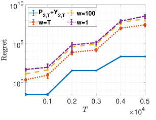
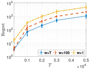
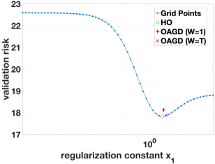
Figure 1 (left and middle) shows the variation $P_{2,T}+Y_{2,T}$ and the regret bound of OAGD with three different window sizes $w\in\{1,100,T\}$ on synthetic data. We observe that OAGD with $w=T$ performs the best, with a gradual decrease in performance as $w$ decreases to $100$ and $w=1$. Additionally, Figure 1 (right) demonstrates (using a 1-dimensional hyperparameter setting) that the performance of OAGD is comparable to the performance of the offline HO (Franceschi et al., 2018).

4.2 Online Parametric Loss Tuning for Imbalanced Data

Imbalanced datasets are common in modern machine learning, posing challenges in generalization and fairness due to underrepresented classes and sensitive attributes. This issue is exacerbated by deep neural networks’ tendency to overfit, appearing accurate and fair during training but performing poorly during testing. Next, we investigate an online HO framework (an online variant of (Li et al., 2021)), which automatically designs a parametric training loss by learning the hyperparameters of a parametric cross-entropy loss to balance accuracy and fairness objectives.

The bilevel objective function for loss tuning is the same as (19) but the leader’s and the follower’s loss functions are defined differently. At each round or timestep $t$, new samples $({\bf{a}}_{t},b_{t})\in\mathcal{D}_{t}:=\{\mathcal{D}^{\text{val}}_{t},\mathcal{D}^{\text{tr}}_{t}\}$ for all $t\in[T]$ are received, where ${\bf{a}}_{t}\in{\mathbb{R}}^{d_{2}}$ represents the feature vector and $b_{t}\in\{1,\ldots,k\}$ represents the corresponding label. For a new sample $({\bf{a}}_{t},b_{t})$, the follower suffers from a parametric cross-entropy loss:

$$g({\bf{x}}_{t-1},{\bf{y}}_{t};\mathcal{D}^{\text{tr}}_{t})=-\log\frac{e^{\gamma_{b_{t}}{\bf{y}}_{t}({\bf{a}}_{t})_{b_{t}}+\Delta_{b_{t}}}}{\sum_{j=1}^{J}e^{\gamma_{j}{\bf{y}}_{t}({\bf{a}}_{t})_{j}+\Delta_{j}}},$$ (20a)

where $${\bf{x}}_{t-1}:=(\Delta_{j},\gamma_{j})$$ are the logit hyperparameters. The leader suffers from a balanced cross entropy loss

$$f({\bf{y}}_{t}({\bf{x}}_{t});\mathcal{D}^{\text{val}}_{t})=-u_{b_{t}}\log\frac{e^{{\bf{y}}_{t}({\bf{a}}_{t})_{b_{t}}}}{\sum_{j=1}^{J}e^{{\bf{y}}_{t}({\bf{a}}_{t})_{b_{t}}}},$$ (20b)

where $u_{j}$ represents the reciprocal of the proportion of samples from the $j$-th class to the total number of samples (Li et al., 2021). There might be one notation abuse here that we need to clarify: ${\bf{y}}_{t}({\bf{x}}_{t})$ still indicates that the follower ${\bf{y}}_{t}$ is conditioned on the leader ${\bf{x}}_{t}$, whereas ${\bf{y}}_{t}({\bf{a}}_{t})_{b_{t}}$ means the predicted logit for class $b_{t}$ that the follower ${\bf{y}}_{t}$ makes on sample ${\bf{a}}_{t}$. Note that the backbone model for ${\bf{y}}_{t}$ is a 4-layer CNN, resulting in a nonconvex bilevel objective. For more details, refer to the Appendix.

Figure 2: Performance comparison (mean$\pm$std) on parametric loss tuning for imbalanced MNIST data across five runs. We compare our OAGD ($w=5,10$) with AutoBalance and Single-Level OGD. OAGD achieves a balanced accuracy comparable to AutoBalance (Li et al., 2021) but with reduced runtime.

Figure 3: Performance comparison (mean±std) on parametric loss tuning for imbalanced MNIST data across five runs, considering induced distribution shift. OAGD (with $w=10$) shows superior performance during distribution shifts, with smaller $\delta$ values exhibiting reduced impact from these shifts.

We compare Algorithm 1 with the following baselines:

1. Single-Level OGD (Zinkevich, 2003): Updates the model $\mathbf{y}_{t}$ with fixed hyperparameters $\mathbf{x}$ at each timestep on the newly observed data using gradient descent.

2. AutoBalance (Li et al., 2021): An offline bilevel gradient descent framework that updates hyperparameters $\mathbf{x}_{t}$ and the model $\mathbf{y}_{t}$ to address imbalance issues.

Figure 4: Performance comparison (mean$\pm$std) on meta-learning for FC100 data across five runs. We compare our OAGD ($w=10$) with ANIL and ITD-BiO. OAGD achieves better accuracy with a shorter runtime.

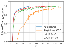
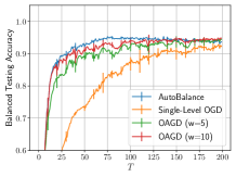
We conducted experiments using the MNIST dataset (LeCun et al., 2010). To create an imbalanced scenario, we selected samples in proportions of $0.6^{i}$ from each class ($i=0,\ldots,9$). For online learning, we used a batch size of 128 at each timestep to train our OAGD. If the window size exceeded 1, we combined the current batch with the previous $w-1$ batches for OAGD training. We assessed cumulative runtime, balanced training accuracy, and balanced testing accuracy. To ensure consistency, we maintained a fixed inner-level learning rate of 0.1 for all bilevel algorithms and single-level OGD, with the outer-level learning rate set at $0.001$.

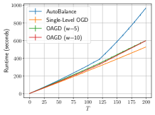
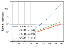
Figure 2 (left) provides runtime comparisons. The Single-Level OGD algorithm is the fastest since it lacks an outer-level training step and trains on a single batch of data at each timestep. Our OAGD exhibits similar runtime characteristics, with the runtime increasing as the window size grows due to more extensive training. In contrast, AutoBalance is the slowest method as it trains on all observed data up to each timestep.

Figure 2 (middle and right) displays balanced training and testing accuracy. AutoBalance quickly achieves high accuracy after 10 timesteps, whereas Single-Level OGD exhibits slower improvement. OAGD ($w=5$) and OAGD ($w=10$) exhibit rapid growth in both testing and training accuracy, eventually outperforming AutoBalance. They benefit from time-smoothing hypergradients. Larger window sizes further enhance OAGD’s balanced training and testing accuracy.

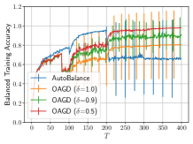
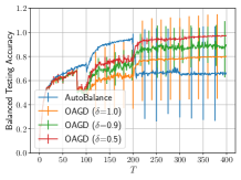
We also conducted experiments to assess method performance under distribution shifts over time, using the MNIST dataset. The experiment spanned 400 timesteps, divided into four phases with varying data distributions, each containing 100 timesteps. Initially, we had a highly imbalanced distribution, with class proportions determined by $0.4^{i}$ for classes where $i$ ranged from $0$ to $9$. This imbalance gradually decreased over the subsequent two phases, transitioning from $0.6^{i}$ to $0.8^{i}$. The final phase with 100 timesteps featured a completely balanced distribution across MNIST’s 10 classes, with normalized proportions (summing to 1) for each class in all four phases.

The parameter $\delta$ controls the attention or weighting assigned to each window. Let’s recall the definition of the “time-averaged hypergradient” from Definition 1 as

$$\tilde{\nabla}F_{t,{\bf{u}}}({\bf{x}},{\bf{y}}):=\frac{1}{W}\sum_{i=0}^{w-1}u_{i}\tilde{\nabla}f_{t-i}({\bf{x}},{\bf{y}}),$$

which is defined using the hypergradients of the losses from the $w$ recent rounds. When $u_{i}$ is set to 1, it calculates the average of a sliding window of online hypergradients during each update. Alternatively, setting $u_{i}=\delta^{i}$ for $\delta\in(0,1)$ assigns more weight to recent values, leading to an exponential average of hypergradients. In our experiment, we set $\delta$ to three values: 1.0, 0.9, and 0.5. A smaller $\delta$ indicates that the algorithm will place more focus on the most recent windows.

The results are shown in Figure 3. As can be seen, Autobalance’s performance drops drastically when the timestep reaches 200. Our OAGD is not affected by the distribution shift too much. A larger window size is advantageous for accurately calculating gradients. However, if the distribution of data shifts over time, using a large window size can result in outdated and inaccurate gradients, which can negatively impact the model’s parameter updating. On the other hand, using a smaller $\delta$ may lead to better performance even when the window size is large as it let the algorithm focus on more recent data windows.

4.3 Online Meta-Learning

Meta-learning aims to bootstrap from a set of given tasks to learn faster on future tasks (Finn et al., 2017; Balcan et al., 2019). A popular formulation is online meta-learning (OML) where agents sequentially face tasks and apply methods such as classical FPL  (Finn et al., 2019) or mirror descent (Denevi et al., 2019) for enhanced meta-learning. We consider an implicit gradient-based OML setting: for each task $\mathcal{T}_{t}$, the follower adapts the leader’s model ${\bf{w}}_{t}\in\mathcal{W}\subset{\mathbb{R}}^{d_{1}}$ using training data $\mathcal{D}^{\text{tr}}_{t}$ with an inner OGD strategy:

$${\bf{u}}^{*}_{t}({\bf{w}}_{t})\in\operatorname*{arg\,min}_{{\bf{u}}}\left\langle{\bf{u}},\nabla f({\bf{w}}_{t};\mathcal{D}^{tr}_{t})\right\rangle+\frac{1}{2\beta}\left\|{\bf{u}}-{\bf{w}}_{t}\right\|^{2},$$

for some $\beta>0$.

Then, the test data $\mathcal{D}^{\text{ts}}_{t}$ will be revealed to the leader for evaluating the performance of the follower’s model ${\bf{u}}^{*}_{t}({\bf{w}}_{t})$. The loss observed at this timestep, denoted as $f({\bf{u}}^{*}_{t}({\bf{w}}_{t});\mathcal{D}^{ts}_{t})$, can then be fed into the leader’s algorithm (outer OGD) to update ${\bf{w}}_{t}$. Despite the convex nature of the loss function, which is a cross-entropy loss, ${\bf{w}}$ represents a 4-layer CNN, ultimately rendering the outer problem nonconvex. Further, the inner problem for loss tuning involves training a CNN and is nonconvex, showing our implementation’s wide scope. We compare our OAGD with the following meta-learning methods:

1. ANIL (Raghu et al., 2019): A widely used meta-learning algorithm, which simplifies MAML by removing the inner loop for all parts of the MAML-trained network except for the task-specific head.

2. ITD-BiO (Ji et al., 2021b): A gradient-based stochastic bilevel optimization framework based on iterative differentiation (ITD).

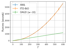
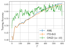
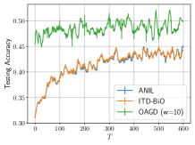
We conduct our experiments using the FC100 (Fewshot-CIFAR100) dataset (Oreshkin et al., 2018) over a 5-way 5-shot task. For the online setting, at each timestep, we only observe one task with 25 (5 way$\times$5 shot) training samples and 25 testing samples. If the window size is greater than 1, we can also utilize data from the previous $w-1$ tasks. In the offline setting where the two baselines are applied, they utilize all the data (tasks) observed until the current timestep for training and testing. The inner and outer learning rates are 0.01 and 5e-5 for ANIL and ITD-BiO, while our OAGD uses the learning rates of 0.1 and 1e-4. These experiments were conducted using a P100 GPU equipped with 12 GB of memory.

In Figure 4, we provide the performance comparison in terms of runtime, training accuracy, and testing accuracy. We compare only our OAGD ($w=10$) to other baselines to enhance the precision of the figure. For the sensitivity analysis concerning the window size, please refer to the Appendix. From the left figure in Figure 4, it’s noticeable that the two baselines consume a similar longer time with an exponential trend, while our OAGD requires the least time, following a linear trend. However, as indicated by the middle and right figures, our OAGD demonstrates competitive training accuracy and even better testing accuracy across all the timesteps, highlighting its superiority.

5 Conclusion

This paper studies online bilevel optimization and provides regret guarantees under different convexity assumptions on the time-varying objective functions. In particular, we propose a new class of online bilevel algorithms capable of leveraging smoothness and providing regret bound in terms of problem-dependent quantities, such as the path-length of the comparator sequence.

Acknowledgements

This work was supported by ARO YIP award W911NF1910027, NSF CAREER award CCF1845076, and NIH grants U01 AG066833, U01 AG068057, and RF1 AG063481.

 

Supplementary Materials for                                                                                        Online Bilevel Optimization: Regret Analysis of Online Alternating Gradient Methods

 

Roadmap. The appendix is organized as follows:

• Appendix A provides some preliminaries on online optimization and a summary of notations used in the appendix.

• Appendix B discusses additional related work on online single-level optimization and offline bilevel optimization.

• Appendix C gives an addendum to Section 3:

  • Appendix C.1 provides the lower bound of OBO (proof of Theorem 5).

  • Appendix C.2 gives the proof for strongly convex OBO with partial information in both dynamic (proof of Theorem 4) and static (proof of Theorem 6) settings.

  • Appendix C.3 gives the proof for convex OBO with partial information in both dynamic (proof of Theorem 7) and static (proof of Theorem 8) settings.

  • Appendix C.4 provides the proof for non-convex OBO with partial information (proof of Theorem 9).

• Appendix D details the implementation and includes additional experiments:

  • Appendix D.1 gives details on online parametric loss tuning experiments as well as additional experiments.

  • Appendix D.2 provides details of online meta-learning experiments as well as additional experiments.

  • Appendix D.3 presents the numerical sensitivity of algorithms to window size and learning rate.

Table 2: Summary of the Notations

Notation	Description
$t$	Time (round) index
$K_{t}$	The number of inner iterations at each round $t$
$T$	The total number of rounds
$\alpha$	Outer stepsize
$\beta$	Inner stepsize
${\bf{x}}_{t}$	Leader’s decision at round $t$
$f_{t}$	Leader’s objective at round $t$
${\bf{y}}_{t}$	Follower’s decision at round $t$
$g_{t}$	Follower’s objective at round $t$
${\bf{x}}_{t}^{*}$	Leader’s optimal decision in the dynamic setting at round $t$: ${\bf{x}}_{t}^{*}\in\operatorname*{arg\,min}_{{\bf{x}}\in\mathcal{X}}f_{t}({\bf{x}})$
${\bf{x}}^{*}$	Leader’s optimal decision in static setting: ${\bf{x}}^{*}\in\operatorname*{arg\,min}_{{\bf{x}}\in\mathcal{X}}\sum_{t=1}^{T}f_{t}({\bf{x}})$
${\bf{y}}_{t}^{*}({\bf{x}})$	Follower’s optimal decision at round $t$ for a given ${\bf{x}}$
$\nabla h_{t}$, $\nabla_{{\bf{xy}}}^{2}h_{t}$, $\nabla_{{\bf{y}}}^{2}h_{t}$	Gradient, Jacobian, and Hessian of $h_{t}$
$\tilde{\nabla}f_{t}({\bf{x}},{\bf{y}}_{t})$	An approximation of the hypergradient $\nabla f_{t}({\bf{x}},{\bf{y}}^{*}_{t}({\bf{x}}))$
$W$, $w$	$W=\sum_{i=0}^{w-1}u_{i}$ for $\{u_{i}\}_{i=0}^{w-1}$ with $1=u_{0}\geq u_{1}\ldots u_{w-1}>0$ and window size $w\in[T]$
$\tilde{\nabla}F_{t,{\bf{u}}}({\bf{x}},{\bf{y}})$	Approximate time-averaged hypergradient: $\tilde{\nabla}F_{t,{\bf{u}}}({\bf{x}},{\bf{y}})=\frac{1}{W}\sum_{i=0}^{w-1}u_{i}\tilde{\nabla}f_{t-i}({\bf{x}},{\bf{y}})$
$\nabla F_{t,{\bf{u}}}({\bf{x}}_{t},{\bf{y}}_{t}^{*}({\bf{x}}_{t}))$	Exact time-averaged hypergradient: $F_{t,{\bf{u}}}({\bf{x}}_{t},{\bf{y}}_{t}^{*}({\bf{x}}_{t}))=\frac{1}{W}\sum_{i=0}^{w-1}u_{i}f_{t-i}({\bf{x}}_{t},{\bf{y}}^{*}_{t}({\bf{x}}_{t}))$
$\left\lVert\cdot\right\rVert$	The Euclidean norm
$D$	The (2-norm) diameter of $\mathcal{X}$: $D=\max_{{\bf{x}},{\bf{x}}^{\prime}\in\mathcal{X}}\|{\bf{x}}-{\bf{x}}^{\prime}\|$
$M$	Upper bound on the outer function: $|f_{t}|\leq M$
$M_{f}$	Difference between $\tilde{\nabla}f_{t}({\bf{x}},{\bf{y}}_{t})$ and $\nabla f_{t}({\bf{x}},{\bf{y}}^{*}_{t}({\bf{x}}))$ w.r.t. $\|{\bf{y}}^{*}_{t}({\bf{x}})-{\bf{y}}_{t}\|$
$L_{\bf{y}}$	Lipschitz constant of ${\bf{y}}^{*}_{t}({\bf{x}})$
$L_{f}$	Lipschitz constant of $\nabla f_{t}({\bf{x}})$
$F_{T}$	Outer function value at the optimum: $\sum_{t=1}^{T}f_{t}({\bf{x}}^{*}_{t},{\bf{y}}^{*}_{t}({\bf{x}}^{*}_{t}))$
$P_{p,T}$	Path-length of the outer minimizers: $\sum_{t=2}^{T}\|{\bf{x}}^{*}_{t-1}-{\bf{x}}^{*}_{t}\|^{p}$
$Y_{p,T}$	Path-length of the inner minimizers: $\sum_{t=2}^{T}\left\lVert{\bf{y}}_{t-1}^{*}({\bf{x}}^{*}_{t-1})-{\bf{y}}_{t}^{*}({\bf{x}}^{*}_{t})\right\rVert^{p}$
$S_{p,T}$	The summation of the inner and outer path-lengths as $S_{p,T}=P_{p,T}+Y_{p,T}$
$\bar{Y}_{p,T}$	The static variant of $Y_{p,T}$: $\sum_{t=2}^{T}\left\lVert{\bf{y}}_{t-1}^{*}({\bf{x}}^{*})-{\bf{y}}_{t}^{*}({\bf{x}}^{*})\right\rVert^{p}$
$H_{p,T}$	Inner minimizer function variation: $\sum_{t=2}^{T}\sup_{{\bf{x}}\in{\mathbb{R}}^{d_{1}}}\|{\bf{y}}^{*}_{t-1}({\bf{x}})-{\bf{y}}^{*}_{t}({\bf{x}})\|^{p}$
$V_{T}$	Online functions variation: $\sum_{t=2}^{T}\sup_{{\bf{x}}\in\mathcal{X}}|f_{t-1}({\bf{x}})-f_{t}({\bf{x}})|$
$G_{T}$	Online gradients variation: $\sum_{t=2}^{T}\sup_{{\bf{x}}\in\mathcal{X}}\left\lVert\nabla f_{t-1}({\bf{x}})-\nabla f_{t}({\bf{x}})\right\rVert^{2}$
$\textnormal{D-Reg}_{T}$	(single-level) dynamic regret: $\sum_{t=1}^{T}f_{t}({\bf{x}}_{t})-\sum_{t=1}^{T}f_{t}({\bf{x}}^{*}_{t})$
$\textnormal{S-Reg}_{T}$	(single-level) static regret: $\sum_{t=1}^{T}f_{t}({\bf{x}}_{t})-\min_{{\bf{x}}\in\mathcal{X}}\sum_{t=1}^{T}f_{t}({\bf{x}})$
$\textnormal{L-Reg}_{T}$	(single-level) local regret: $\sum_{t=1}^{T}\left\|\nabla F_{t,{\bf{u}}}({\bf{x}}_{t})\right\|^{2}$
$\textnormal{BD-Reg}_{T}$	Bilevel dynamic regret: $\sum_{t=1}^{T}f_{t}({\bf{x}}_{t},{\bf{y}}_{t}^{*}({\bf{x}}_{t}))-\sum_{t=1}^{T}f_{t}({\bf{x}}^{*}_{t},{\bf{y}}^{*}_{t}({\bf{x}}^{*}_{t}))$
$\textnormal{BS-Reg}_{T}$	Bilevel (outer) static regret: $\sum_{t=1}^{T}f_{t}({\bf{x}}_{t},{\bf{y}}_{t}^{*}({\bf{x}}_{t}))-\min_{{\bf{x}}\in\mathcal{X}}\sum_{t=1}^{T}f_{t}({\bf{x}},{\bf{y}}^{*}_{t}({\bf{x}}))$
$\textnormal{BL-Reg}_{T}$	Bilevel local regret: $\sum_{t=1}^{T}\left\|\nabla F_{t,{\bf{u}}}({\bf{x}}_{t},{\bf{y}}_{t}^{*}({\bf{x}}_{t}))\right\|^{2}$

Appendix A Addendum to Section 1: Preliminaries and Notations

We provide several technical lemmas used in the proofs. We start by assembling some well-known facts about convex and smooth functions.

1. (Smoothness): Suppose $f({\bf{x}})$ is $L$-smooth. Then, by definition, the following inequalities hold for any two points ${\bf{x}},{\bf{y}}\in\mathbb{R}^{d}$:

   $$\|\nabla f({\bf{x}})-\nabla f({\bf{y}})\|\leq L\|{\bf{x}}-{\bf{y}}\|,\,$$ (21)

   $$f({\bf{y}})-f({\bf{x}})\leq\langle{\bf{y}}-{\bf{x}},\nabla f({\bf{x}})\rangle+\frac{L}{2}{\|{\bf{y}}-{\bf{x}}\|}^{2}.$$

   Further, if $${\bf{x}}^{*}\in\operatorname*{arg\,min}_{{\bf{x}}\in{\mathbb{R}}^{d}}f({\bf{x}})$$, then

   $${\|\nabla f({\bf{y}})\|}^{2}\leq 2L(f({\bf{y}})-f({\bf{x}}^{*})).$$

2. (Smoothness and Convexity): Suppose $f({\bf{x}})$ is $L$-smooth and convex. Then, the following holds for any two points ${\bf{x,y}}\in\mathbb{R}^{d}$:

   $$\langle\nabla f({\bf{y}})-\nabla f({\bf{x}}),{\bf{y}}-{\bf{x}}\rangle\geq\frac{1}{L}{\|\nabla f({\bf{y}})-\nabla f({\bf{x}})\|}^{2}.$$

3. (Strong-Convexity): Suppose $f({\bf{x}})$ is $\mu$-strongly convex. Then, by definition, the following inequality holds for any two points ${\bf{x,y}}\in\mathbb{R}^{d}$:

   $$f({\bf{y}})-f({\bf{x}})\geq\langle{\bf{y}}-{\bf{x}},\nabla f({\bf{x}})\rangle+\frac{\mu}{2}{\|{\bf{y}}-{\bf{x}}\|}^{2}.$$ (22)

   Using the above inequality, one can conclude that

   $$\langle\nabla f({\bf{y}})-\nabla f({\bf{x}}),{\bf{y}}-{\bf{x}}\rangle\geq\mu{\|{\bf{y}}-{\bf{x}}\|}^{2}.$$

The following lemma provides the self-bounding property of smooth functions.

Lemma 10.

[Srebro et al., 2010, Lemma 3.1] For a non-negative and $L$–smooth function $f:\mathcal{X}\rightarrow{\mathbb{R}}$, we have

$$\left\lVert\nabla f({\bf{x}})\right\rVert\leq\sqrt{4Lf({\bf{x}})},\ \forall{\bf{x}}\in\mathcal{X}.$$

Lemma 11.

[Nesterov, 2003, Theorem 2.1.11] Let $g:\mathbb{R}^{d}\rightarrow\mathbb{R}$ be a function that is smooth, $\mu_{g}$-strongly convex, and $L_{g}$-gradient Lipschitz continuous on an open convex set $\mathcal{Y}\subseteq\mathbb{R}^{d}$. Suppose that $g$ has a global minimizer ${\bf{y}}^{*}$ over $\mathcal{Y}$. Then, the sequence $\{{\bf{y}}_{t}\}_{t=1}^{T}$ generated by the gradient descent method ${\bf{y}}_{t+1}={\bf{y}}_{t}-\beta\nabla g({\bf{y}}_{t})$ with stepsize $\beta\in(0,2/(\mu_{g}+L_{g})]$ satisfies

$$\|{\bf{y}}_{t+1}-{\bf{y}}^{*}\|^{2}\leq\left(1-\frac{2\beta\mu_{g}L_{g}}{\mu_{g}+L_{g}}\right)\|{\bf{y}}_{t}-{\bf{y}}^{*}\|^{2}.$$

If $\beta=2/(\mu_{g}+L_{g})$, then

$$\|{\bf{y}}_{t+1}-{\bf{y}}^{*}\|^{2}\leq\left(\frac{\kappa_{g}-1}{\kappa_{g}+1}\right)^{2}\|{\bf{y}}_{t}-{\bf{y}}^{*}\|^{2},$$

where $\kappa_{g}=L_{g}/\mu_{g}$.

Lemma 12.

For any set of vectors $\{{\bf{x}}_{i}\}_{i=1}^{m}$ with ${\bf{x}}_{i}\in\mathbb{R}^{d}$, we have

$$\left\|\sum\limits_{i=1}^{m}{\bf{x}}_{i}\right\|^{2}\leq m\sum\limits_{i=1}^{m}{\|{\bf{x}}_{i}\|}^{2}.$$

Lemma 13.

For all $T\in{\mathbb{N}}$,

1. $\log(T)+\frac{1}{T}\leq\sum_{t=1}^{T}\frac{1}{t}\leq\log(T)+1;$

2. $\sum_{t=1}^{T}\frac{1}{\sqrt{t}}\leq 2\sqrt{T};$

3. If $1<s<\infty$, then $\xi(s)=\sum_{t=1}^{T}1/t^{s}$ is called the Riemann $\xi$-function and we have

   $$\xi(2n)=(-1)^{n+1}\frac{(2\pi)^{2n}B_{2n}}{2(2n)!},~{}~{}~{}~{}n=1,2,3,\ldots,$$

   where the coefficients $B_{2n}$ are the Bernoulli numbers.

Lemma 14.

For any ${\bf{x}},{\bf{y}},{\bf{z}}\in\mathbb{R}^{d}$, the following holds for any $c>0:$

$${\|{\bf{x}}+{\bf{y}}\|}^{2} \leq(1+c){\|{\bf{x}}\|}^{2}+\left(1+\frac{1}{c}\right){\|{\bf{y}}\|}^{2},~{}~{}\textnormal{and}$$

$$\left\lVert{\bf{x}}-{\bf{y}}\right\rVert^{2} \geq(1-c)\left\lVert{\bf{x}}-{\bf{z}}\right\rVert^{2}+\left(1-\frac{1}{c}\right)\left\lVert{\bf{z}}-{\bf{y}}\right\rVert^{2}.$$

Lemma 15.

[Shalev-Shwartz et al., 2011, Lemma 2.8] Let $\mathcal{X}\subseteq\mathbb{R}^{d}$ be a nonempty convex set. Let $f({\bf{x}}):\mathcal{X}\rightarrow\mathbb{R}$ be a $\mu_{f}$-strongly convex function over $\mathcal{X}$. Let ${\bf{x}}^{*}\in\operatorname*{arg\,min}_{{\bf{x}}\in\mathcal{X}}\{f({\bf{x}})\}$. Then, for any ${\bf{y}}\in\mathcal{X}$, we have

$$f({\bf{x}}^{*})-f({\bf{y}})\leq-\frac{\mu_{f}}{2}\|{\bf{y}}-{\bf{x}}^{*}\|^{2}.$$

A.1 On the Comparability of Dynamic Metrics

The following example shows that $P_{p,T}$, $Y_{p,T}$, and $\bar{Y}_{p,T}$ are not comparable in general and all three measures play a key role in OBO.

Example 1.

Let $\mathcal{X}=\left[-1,1\right]$ and consider a sequence of quadratic cost functions

$$f_{t}({\bf{x}},{\bf{y}}) =\frac{1}{2}({\bf{x}}+2a_{t}^{(1)})^{2}+\frac{1}{2}({\bf{y}}-a_{t}^{(2)})^{2}+a_{t}^{(3)},$$

$$g_{t}({\bf{x}},{\bf{y}}) =\frac{1}{2}{\bf{y}}^{2}-({\bf{x}}-a_{t}^{(2)}){\bf{y}}+a_{t}^{(4)},$$

for all $t\in[T]$, where $\{a_{t}^{(i)}\}_{i=1}^{4}$ are some time-varying constants.

It follows from (3b) that

$${\bf{y}}^{*}_{t}({\bf{x}}_{t})={\bf{x}}_{t}-a_{t}^{(2)},\qquad{\bf{x}}_{t}^{*}=-a_{t}^{(1)}+a_{t}^{(2)},\qquad{\bf{y}}^{*}_{t}({\bf{x}}_{t}^{*})=a_{t}^{(1)}.$$

Let $a_{t}^{(2)}=(-1)^{t}/\sqrt{t}$ for all $t\in[T]$.

• If $a_{t}^{(1)}=a_{t}^{(2)}$, then $P_{1,T}=P_{2,T}=0$, $Y_{1,T}=\bar{Y}_{1,T}=\mathcal{O}(\sqrt{T})$, and $Y_{2,T}=\bar{Y}_{2,T}=\mathcal{O}(\log{T})$.

• If $a_{t}^{(1)}=0$, then $P_{1,T}=\mathcal{O}(\sqrt{T})$, $P_{2,T}=\mathcal{O}(\log{T})$, and $Y_{1,T}=Y_{2,T}=0$.

This shows that $S_{1,T}=P_{1,T}+Y_{2,T}$, $S_{2,T}=P_{2,T}+Y_{2,T}$ are not comparable in general. Similarly, static metrics $\bar{Y}_{1,T}$ and $\bar{Y}_{2,T}$ are not comparable.

Appendix B Addendum to Section 2: Additional Related Work

Online learning and stochastic optimization are closely related. The key difference between them is that at each round $t$ of the online optimization, the loss function can be arbitrarily chosen by the adversary. Given the vastness of the online and stochastic optimization literature, we do not strive to provide an exhaustive review. Instead, we mainly focus on a few representative works on online static and worst-case dynamic regret minimization, as well as bilevel optimization. Refer to [Hazan, 2016a, Hoi et al., 2021] and [Liu et al., 2021, Sinha et al., 2017] for surveys on online and bilevel optimization, respectively.

Static Regret Minimization:

In single-level online optimization, the goal of the player (learner) is to choose a sequence $\{{\bf{x}}_{t}\}_{t=1}^{T}$ such that her regret is minimized. There are different notions of regret in the literature including static, dynamic (defined in (1)), and adaptive [Hazan, 2016b, Shalev-Shwartz, 2007, Shalev-Shwartz et al., 2011]. In the case of static regret, ${\bf{x}}^{\ast}_{t}$ is replaced by ${\bf{x}}^{\ast}\in\operatorname*{arg\,min}_{{\bf{x}}\in\mathcal{X}}\sum_{t=1}^{T}f_{t}({\bf{x}})$. This type of regret is well-studied in the literature of online learning [Hazan, 2016b, Shalev-Shwartz, 2007, Shalev-Shwartz et al., 2011]. Zinkevich [2003] shows that online gradient descent (OGD) provides a $\mathcal{O}(\sqrt{T})$ regret bound for convex (possibly nonsmooth) functions. Hazan et al. [2007] improves this bound to $\mathcal{O}(\log T)$ for strongly-convex functions. These results were also shown to be minimax optimal [Abernethy et al., 2008]. Zhou et al. [2020b] provides regret bounds for online learning algorithms under relative Lipschitz and/or relative strongly-convexity assumptions.

In addition to exploiting convexity of the online functions, there are recent studies improving static regret by incorporating smoothness [Chiang et al., 2012, Srebro et al., 2010]. These problem-dependent bounds can safeguard the worst-case minimax rate yet be much better in easy cases of online learning problems (e.g., loss functions with a small deviation). For instance, [Srebro et al., 2010] shows that for convex smooth non-negative functions, OGD can achieve an $\mathcal{O}(1+\sqrt{F_{T}})$ small-loss regret bound, where $F_{T}=\sum_{t=1}^{T}f_{t}({\bf{x}}^{*})$ and ${\bf{x}}^{\ast}\in\operatorname*{arg\,min}_{{\bf{x}}\in\mathcal{X}}\sum_{t=1}^{T}f_{t}({\bf{x}})$. For convex smooth functions, [Chiang et al., 2012] establishes an $\mathcal{O}(1+\sqrt{G_{T}})$ bound, where $G_{T}=\sum_{t=2}^{T}\sup_{{\bf{x}}\in\mathcal{X}}\left\lVert\nabla f_{t-1}({\bf{x}})-\nabla f_{t}({\bf{x}})\right\rVert^{2}$ is the gradient variation. These bounds are particularly favored in slowly changing environments in which the online functions evolve gradually [Zhao et al., 2020].

Dynamic Regret Minimization:

Single-level dynamic regret forces the player to compete with time-varying comparators, and thus is particularly favored in non-stationary environments [Sugiyama and Kawanabe, 2012]. The notion of dynamic regret is also referred to as tracking regret or shifting regret in the prediction with expert advice setting [Bousquet and Warmuth, 2002, Herbster and Warmuth, 1998, 2001, Wei et al., 2016, Zheng et al., 2019]. There are two kinds of dynamic regret in previous studies: The universal dynamic regret aims to compare with any feasible comparator sequence [Zhang et al., 2018a, Zhao et al., 2020, Zinkevich, 2003], while the worst-case dynamic regret (defined in (1)) specifies the comparator sequence to be the sequence of minimizers of online functions [Aydore et al., 2019, Besbes et al., 2015, Jadbabaie et al., 2015, Mokhtari et al., 2016, Yang et al., 2016, Zhang et al., 2017]. We present related works for the latter case as it is the setting studied in this paper.

It is known that in the worst case, sublinear dynamic regret is not attainable unless one imposes regularity of some form on the comparator sequence or the function sequence [Besbes et al., 2015, Hall and Willett, 2015, Jadbabaie et al., 2015]. Yang et al. [2016] shows that OGD enjoys an $\mathcal{O}(1+\sqrt{TP_{1,T}})$ worst-case dynamic regret bound for convex functions when the path-length $P_{1,T}$ is known. For strongly convex and smooth functions, [Mokhtari et al., 2016] shows that an $\mathcal{O}(1+P_{1,T})$ dynamic regret bound is achievable. Chang and Shahrampour [2021] proves that OGD can achieve an $\mathcal{O}(1+P_{2,T})$ regret bound without the bounded gradient assumption. Zhang et al. [2017] further proposes the online multiple gradient descent algorithm and proves that the algorithm enjoys an $\mathcal{O}(1+\min\{P_{1,T},P_{2,T}\})$ regret bound; this bound has been recently enhanced to $\mathcal{O}(1+\min\{P_{1,T},P_{2,T},V_{T}\})$ by an improved analysis [Zhao and Zhang, 2021], where $V_{T}=\sum_{t=2}^{T}\sup_{{\bf{x}}\in\mathcal{X}}|f_{t-1}({\bf{x}})-f_{t}({\bf{x}})|$. Yang et al. [2016] further shows that the $\mathcal{O}(1+P_{2,T})$ rate is attainable for convex and smooth functions, provided that all the minimizers ${\bf{x}}^{*}_{t}$ lie in the interior of the domain $\mathcal{X}$. The above results use path-length (or squared path-length) as the regularity, which is in terms of the trajectory of the comparator sequence. Nazari et al. [2019, 2022] extend the above results to the distributed settings and provide dynamic regret bounds in terms of the $\ell_{1}$ path-length. Besbes et al. [2015] shows that OGD with a restarting strategy attains an $\mathcal{O}(1+T^{2/3}{V_{T}}^{1/3})$ regret for convex functions when $V_{T}$ is available, which has been recently improved to $\mathcal{O}(1+T^{1/3}{V_{T}}^{2/3})$ for the square loss [Baby and Wang, 2019].

Adaptive Regret:

Adaptive regret [Daniely et al., 2015, Hazan and Seshadhri, 2007, Zhang et al., 2019, 2020, 2018b] is also used to capture the dynamics in the environment. Specifically, it characterizes a local version of static regret, where

$$\mbox{Regret}_{T}([r,s])\triangleq\sum_{t=r}^{s}f_{t}({\bf{x}}_{t})-\min_{{\bf{x}}\in\mathcal{X}}\sum_{t=r}^{s}f_{t}({\bf{x}}),$$

for each interval $[r,s]\subseteq[T]$. Zhang et al. [2018b] provides a connection between strongly adaptive regret and dynamic regret and proposes an adaptive algorithm which can bound the dynamic regret without prior knowledge of the functional variation. Zhang et al. [2020] develops a new algorithm which can minimize the dynamic regret and the adaptive regret simultaneously.

Local Regret Minimization:

Non-convex online optimization is a more challenging setting than the convex case. Some notable works in the non-convex literature include adversarial multi-armed bandit with a continuum of arms [Bubeck et al., 2008, Héliou et al., 2020, 2021, Krichene et al., 2015] and classical Follow-the-Perturbed-Leader algorithm with access to an offline non-convex optimization oracle [Agarwal et al., 2019, Kleinberg et al., 2008, Suggala and Netrapalli, 2020]. Hazan et al. [2017] introduces a local regret measure based on gradients of the loss to address intractable non-convex online models. Their regret is local in the sense that it averages a sliding window of gradients and quantifies the objective of predicting points with small gradients on average. They are motivated by a game-theoretic perspective, where an adversary reveals observations from an unknown static loss. The gradients of the loss functions from the $w$ most recent rounds of play are evaluated at the current model parameters ${\bf{x}}_{t}$, and these gradients are then averaged. The motivation behind averaging is two-fold: (i) a randomly selected update has a small time-averaged gradient in expectation if an algorithm incurs local regret sublinear in $T$, and (ii) for any online algorithm, an adversarial sequence of loss functions can force the local regret incurred to scale with $T$ as $\mathcal{O}(T/w^{2})$. Hallak et al. [2021] extends the local regret minimization to online, non-smooth, non-convex problems. These arguments, presented in [Aydore et al., 2019, Hallak et al., 2021, Hazan et al., 2017, Nazari et al., 2022], inspire our use of local regret for OBO.

(Offline) Bilevel Optimization:

Since its first formulation by Stackelberg [von Stackelberg, 1952] and the first mathematical model by Bracken and McGill [Bracken and McGill, 1973], there has been a significant growth in applications and developments of bilevel programming. Existing works either reduce the problem to a single-level optimization problem [Aiyoshi and Shimizu, 1984, Al-Khayyal et al., 1992, Edmunds and Bard, 1991, Hansen et al., 1992, Lv et al., 2007, Moore, 2010, Shi et al., 2005, Sinha et al., 2017] or apply an (alternating) optimization method to solve the original problem. The single-level formulations, using the Karush-Kuhn-Tucker (KKT) conditions or penalty approaches, are generally difficult to solve [Sinha et al., 2017].

Gradient-based approaches are more attractive for bilevel programming due to their simplicity and effectiveness. This type of approach estimates the hypergradients for iterative updates, and can generally be divided into two categories: approximate implicit differentiation (AID) and iterative differentiation (ITD) classes. ITD-based approaches [Finn et al., 2017, Franceschi et al., 2017, Grazzi et al., 2020, Maclaurin et al., 2015] estimate the hypergradient in either a reverse (automatic differentiation) or forward manner. AID-based approaches [Domke, 2012, Grazzi et al., 2020, Ji et al., 2021b, Pedregosa, 2016] estimate the hypergradient via implicit differentiation. Franceschi et al. [2018] characterized the asymptotic convergence of a backpropagation-based approach as one of ITD-based algorithms by assuming the inner-level problem is strongly convex. Shaban et al. [2019] provided a similar analysis for a truncated backpropagation scheme. Li et al. [2020], Liu et al. [2020] analyzed the asymptotic performance of ITD-based approaches when the inner-level problem is convex.

Finite-time complexity analysis for bilevel optimization has also been explored. Ghadimi and Wang [2018] provided a finite-time convergence analysis for an AID-based algorithm under different loss geometries: The outer function is strongly convex, convex or non-convex, and the inner function is strongly convex. Ji et al. [2021b] provided an improved finite-time analysis for both AID- and ITD-based algorithms under the nonconvex-strongly-convex geometry. Liang et al. [2023] provided the lower bounds on complexity as well as upper bounds under these two geometries. When the objective functions can be expressed in an expected or finite-time form, [Ghadimi and Wang, 2018, Hong et al., 2023, Ji et al., 2021b] developed stochastic bilevel algorithms and provided the finite-time analysis. There have been subsequent studies on accelerating SGD-type bilevel optimization via momentum and variance reduction techniques [Chen et al., 2022, Guo et al., 2021, Huang and Huang, 2021, Ji et al., 2021a] as well. However, a fundamental assumption in all the aforementioned works is that the cost function does not change throughout the horizon over which we seek to optimize it.

Appendix C Addendum to Section 3: Proof of Main Theorems

C.1 Proof of Theorem 5

Proof.

We randomly generate a sequence of functions $\{(f_{t},g_{t})\}_{t=1}^{T}$ and show that there exists a distribution of online functions such that for any bilevel algorithm $\mathcal{A}$, we have ${\mathbb{E}}\left[\textnormal{BD-Reg}_{T}\right]\geq{\mathbb{E}}[S_{2,T}]$. Specifically, for any bilevel algorithm $\mathcal{A}$ that generates a sequence of $\{{\bf{x}}_{t}\}_{t=1}^{T}$, we consider the expected regret as follows:

$${\mathbb{E}}\left[\textnormal{BD-Reg}_{T}\right]={\mathbb{E}}\left[\sum_{t=1}^{T}f_{t}({\bf{x}}_{t},{\bf{y}}_{t}^{*}({\bf{x}}_{t}))-\sum_{t=1}^{T}f_{t}({\bf{x}}^{*}_{t},{\bf{y}}^{*}_{t}({\bf{x}}^{*}_{t}))\right].$$

Let $d_{1}=d_{2}=1$ and $\mathcal{X}=\mathbb{R}$. For each round $t$, we randomly sample ${\bf{a}}_{t}^{(1)}$ and ${\bf{a}}_{t}^{(2)}$ from the Gaussian distribution $\mathcal{N}(0,1)$. For all $t\in[T]$, let

$$f_{t}({\bf{x}},{\bf{y}}_{t}^{*}({\bf{x}})) =6\left({\bf{y}}_{t}^{*}({\bf{x}})-\left({\bf{a}}_{t}^{(1)}+{\bf{a}}_{t}^{(2)}\right)\right)^{2}+6\left({\bf{x}}-{\bf{a}}_{t}^{(1)}\right)^{2},$$

$$\textnormal{s.t.}~{}~{}~{}{\bf{y}}_{t}^{*}({\bf{x}}) \in\operatorname*{arg\,min}_{{\bf{y}}\in{\mathbb{R}}^{d_{2}}}g_{t}({\bf{x}},{\bf{y}})=\frac{1}{2}{\bf{y}}^{2}-\left({\bf{x}}+{\bf{a}}_{t}^{(2)}\right){\bf{y}}.$$

It follows from (3b) that

$${\bf{y}}^{*}_{t}({\bf{x}}_{t})={\bf{x}}_{t}+{\bf{a}}_{t}^{(2)},\quad{\bf{x}}_{t}^{*}={\bf{a}}_{t}^{(1)},\quad\textnormal{and}\quad{\bf{y}}^{*}_{t}({\bf{x}}_{t}^{*})={\bf{a}}_{t}^{(1)}+{\bf{a}}_{t}^{(2)}.$$

Notice that ${\bf{x}}_{t}\in\mathcal{X}$, $t\in[T]$, is independent from ${\bf{a}}_{t}^{(1)}$. Hence,

$$\begin{split}{\mathbb{E}}\left[\textnormal{BD-Reg}_{T}\right]&=6\sum_{t=1}^{T}{\mathbb{E}}\left[\left({\bf{x}}_{t}-{\bf{a}}_{t}^{(1)}\right)^{2}\right]\\ &=6\sum_{t=1}^{T}\left({\mathbb{E}}\left[\left({\bf{a}}_{t}^{(1)}\right)^{2}\right]+{\mathbb{E}}\left[{\bf{x}}_{t}^{2}\right]\right)\\ &\geq 6T.\end{split}$$ (23)

For $T\geq 2$, we obtain

$$\begin{split}{\mathbb{E}}\left[S_{2,T}\right]={\mathbb{E}}[P_{2,T}]+{\mathbb{E}}[Y_{2,T}]&=\sum_{t=2}^{T}{\mathbb{E}}\left[\left({\bf{x}}^{*}_{t-1}-{\bf{x}}^{*}_{t}\right)^{2}\right]+\sum_{t=2}^{T}{\mathbb{E}}\left[\left({\bf{y}}_{t-1}^{*}({\bf{x}}^{*}_{t-1})-{\bf{y}}_{t}^{*}({\bf{x}}^{*}_{t})\right)^{2}\right]\\ &=\sum_{t=2}^{T}{\mathbb{E}}\left[\left({\bf{a}}_{t}^{(1)}-{\bf{a}}_{t-1}^{(1)}\right)^{2}\right]+\sum_{t=2}^{T}{\mathbb{E}}\left[\left({\bf{a}}_{t}^{(1)}+{\bf{a}}_{t}^{(2)}-({\bf{a}}_{t-1}^{(1)}+{\bf{a}}_{t-1}^{(2)})\right)^{2}\right]\\ &=\sum_{t=2}^{T}2\left({\mathbb{E}}\left[\left({\bf{a}}_{t}^{(1)}\right)^{2}\right]+{\mathbb{E}}\left[\left({\bf{a}}_{t-1}^{(1)}\right)^{2}\right]\right)+{\mathbb{E}}\left[\left({\bf{a}}_{t}^{(2)}\right)^{2}\right]+{\mathbb{E}}\left[\left({\bf{a}}_{t-1}^{(2)}\right)^{2}\right]\\ &\leq 6(T-1).\end{split}$$ (24)

Here, the third equality follows from the independence of ${\bf{a}}^{(1)}_{t}$ and ${\bf{a}}^{(2)}_{t}$ for all $t\in[T]$.

Now, it follows from (23) and (24) that ${\mathbb{E}}\left[\textnormal{BD-Reg}_{T}\right]\geq{\mathbb{E}}[S_{2,T}]$, and for any given algorithm $\mathcal{A}$, there exists a sequence of functions $\{(f_{t},g_{t})\}_{t=1}^{T}$ such that ${\mathbb{E}}\left[\textnormal{BD-Reg}_{T}\right]=\Omega\left(S_{2,T}\right)$. ∎

C.2 Proof for Strongly Convex OBO with Partial Information

In this section, we provide the dynamic regret bound for strongly convex OBO with partial information. Specifically, we derive a problem-dependent regret bound for Algorithm 1.

C.2.1 Auxiliary Lemmas

Lemma 16 (Restatement of Lemma 3).

Under Assumption A, for all $t\in[T]$, ${\bf{x}},{\bf{x}}^{\prime}\in\mathcal{X}$, and ${\bf{y}}\in{\mathbb{R}}^{d_{2}}$, we have

$$\left\|{\bf{y}}^{*}_{t}({\bf{x}})-{\bf{y}}^{*}_{t}({\bf{x}}^{\prime})\right\|\leq L_{{\bf{y}}}\left\|{\bf{x}}-{\bf{x}}^{\prime}\right\|,$$ (25)

$$\|\tilde{\nabla}f_{t}({\bf{x}},{\bf{y}})-\nabla f_{t}({\bf{x}},{\bf{y}}^{*}_{t}({\bf{x}}))\|\leq M_{f}\left\|{\bf{y}}-{\bf{y}}^{*}_{t}({\bf{x}})\right\|,$$ (26)

$$\left\|\nabla f_{t}({\bf{x}},{\bf{y}}_{t}^{*}({\bf{x}}))-\nabla f_{t}({\bf{x}}^{\prime},{\bf{y}}_{t}^{*}({\bf{x}}^{\prime}))\right\|\leq L_{f}\left\|{\bf{x}}-{\bf{x}}^{\prime}\right\|.$$ (27)

Here, $L_{{\bf{y}}}$, $M_{f}$, and $L_{f}$ are defined in (28), (33), and (35), respectively.

Proof.

The proof is an adaptation of the proof from [Ghadimi and Wang, 2018, Lemma 2.2] to the online setting.

We first show (25). Since ${\bf{y}}^{*}_{t}({\bf{x}})\in\operatorname*{arg\,min}_{{\bf{y}}\in{\mathbb{R}}^{d_{2}}}g_{t}({\bf{x}},{\bf{y}})$, we have

$$\nabla_{{\bf{y}}}g_{t}\left({\bf{x}},{\bf{y}}^{*}_{t}({\bf{x}})\right)=0,\quad\textnormal{and}\quad\nabla^{2}_{{\bf{x}}{\bf{y}}}g_{t}\left({\bf{x}},{\bf{y}}^{*}_{t}({\bf{x}})\right)=0.$$

This together with the chain rule implies that

$$\nabla{\bf{y}}^{*}_{t}({\bf{x}})\nabla^{2}_{{\bf{y}}}g_{t}\left({\bf{x}},{\bf{y}}^{*}_{t}({\bf{x}})\right)+\nabla^{2}_{{\bf{x}}{\bf{y}}}g_{t}\left({\bf{x}},{\bf{y}}^{*}_{t}({\bf{x}})\right)=0.$$

It follows from Assumption A2. that $\nabla^{2}_{{\bf{y}}}g_{t}\left({\bf{x}},{\bf{y}}^{*}_{t}({\bf{x}})\right)$ is positive definite. Hence,

$$\nabla{\bf{y}}^{*}_{t}({\bf{x}})=-\nabla^{2}_{{\bf{x}}{\bf{y}}}g_{t}\left({\bf{x}},{\bf{y}}^{*}_{t}({\bf{x}})\right)\left(\nabla^{2}_{{\bf{y}}}g_{t}\left({\bf{x}},{\bf{y}}^{*}_{t}({\bf{x}})\right)\right)^{-1}.$$

Now, from Assumption A3., we get

$$\begin{split}\left\lVert\nabla{\bf{y}}^{*}_{t}({\bf{x}})\right\rVert&=\left\lVert\nabla^{2}_{{\bf{x}}{\bf{y}}}g_{t}\left({\bf{x}},{\bf{y}}^{*}_{t}({\bf{x}})\right)\left(\nabla^{2}_{{\bf{y}}}g_{t}\left({\bf{x}},{\bf{y}}^{*}_{t}({\bf{x}})\right)\right)^{-1}\right\rVert\\ &\leq\left\lVert\nabla^{2}_{{\bf{x}}{\bf{y}}}g_{t}\left({\bf{x}},{\bf{y}}^{*}_{t}({\bf{x}})\right)\right\rVert\left\lVert\left(\nabla^{2}_{{\bf{y}}}g_{t}\left({\bf{x}},{\bf{y}}^{*}_{t}({\bf{x}})\right)\right)^{-1}\right\rVert\\ &\leq\frac{\ell_{g,1}}{\mu_{g}}=:L_{{\bf{y}}}.\end{split}$$ (28)

Next, we show (26). Let ${\bf{M}}_{t}({\bf{x}},{\bf{y}}):=\nabla^{2}_{{\bf{x}}{\bf{y}}}g_{t}\left({\bf{x}},{\bf{y}}\right)\left(\nabla^{2}_{{\bf{y}}}g_{t}\left({\bf{x}},{\bf{y}}\right)\right)^{-1}$. Define

$$\Delta_{t}:=\nabla f_{t}({\bf{x}},{\bf{y}})-\nabla f_{t}({\bf{x}},{\bf{y}}_{t}^{*}({\bf{x}})),$$

$$\Delta_{t}^{1}:=\nabla_{\bf{x}}f_{t}\left({\bf{x}},{\bf{y}}\right)-\nabla_{\bf{x}}f_{t}\left({\bf{x}},{\bf{y}}^{*}_{t}({\bf{x}})\right),$$

$$\Delta_{t}^{2}:={\bf{M}}_{t}({\bf{x}},{\bf{y}})\nabla_{\bf{y}}f_{t}\left({\bf{x}},{\bf{y}}\right)-{\bf{M}}_{t}({\bf{x}},{\bf{y}}^{*}_{t}({\bf{x}}))\nabla_{\bf{y}}f_{t}\left({\bf{x}},{\bf{y}}^{*}_{t}({\bf{x}})\right),$$

$$\Delta_{t}^{3}:={\bf{M}}_{t}({\bf{x}},{\bf{y}})\{\nabla_{\bf{y}}f_{t}\left({\bf{x}},{\bf{y}}\right)-\nabla f_{t}\left({\bf{x}},{\bf{y}}^{*}_{t}({\bf{x}})\right)\},$$

$$\Delta_{t}^{4}:=\{{\bf{M}}_{t}({\bf{x}},{\bf{y}})-{\bf{M}}_{t}\left({\bf{x}},{\bf{y}}^{*}_{t}({\bf{x}})\right)\}\nabla_{\bf{y}}f_{t}\left({\bf{x}},{\bf{y}}^{*}_{t}({\bf{x}})\right),$$

$$\Delta_{t}^{5}:=\left\{\nabla^{2}_{{\bf{x}}{\bf{y}}}g_{t}\left({\bf{x}},{\bf{y}}\right)-\nabla^{2}_{{\bf{x}}{\bf{y}}}g_{t}\left({\bf{x}},{\bf{y}}^{*}_{t}({\bf{x}})\right)\right\}\left(\nabla^{2}_{{\bf{y}}}g_{t}\left({\bf{x}},{\bf{y}}\right)\right)^{-1},$$

$$\Delta_{t}^{6}:=\nabla^{2}_{{\bf{x}}{\bf{y}}}g_{t}\left({\bf{x}},{\bf{y}}^{*}_{t}({\bf{x}})\right)\left\{\left(\nabla^{2}_{{\bf{y}}}g_{t}\left({\bf{x}},{\bf{y}}\right)\right)^{-1}-\left(\nabla^{2}_{{\bf{y}}}g_{t}\left({\bf{x}},{\bf{y}}^{*}_{t}({\bf{x}})\right)\right)^{-1}\right\},$$

which implies that

$$\Delta_{t} =\Delta_{t}^{1}-\Delta_{t}^{2}=\Delta_{t}^{1}-\Delta_{t}^{3}-\Delta_{t}^{4}=\Delta_{t}^{1}-\Delta_{t}^{3}-(\Delta_{t}^{5}+\Delta_{t}^{6})\nabla_{{\bf{y}}}f_{t}({\bf{x}},{\bf{y}}_{t}^{*}({\bf{x}})).$$ (29)

From Assumption A, we have

$$\|\Delta_{t}^{1}\|\leq\ell_{f,1}\left\|{\bf{y}}-{\bf{y}}^{*}_{t}({\bf{x}})\right\|,\quad\|\Delta_{t}^{3}\|\leq\frac{\ell_{f,1}\ell_{g,1}}{\mu_{g}}\left\|{\bf{y}}-{\bf{y}}^{*}_{t}({\bf{x}})\right\|,\quad\|\Delta_{t}^{5}\|\leq\frac{\ell_{g,2}}{\mu_{g}}\left\|{\bf{y}}-{\bf{y}}^{*}_{t}({\bf{x}})\right\|.$$ (30)

Note that

$$\|A_{2}^{-1}-A_{1}^{-1}\| =\|A_{1}^{-1}(A_{1}-A_{2})A_{2}^{-1}\|\leq\|A_{1}^{-1}\|\|A_{2}^{-1}\|\|A_{1}-A_{2}\|,$$

which implies that

$$\|\Delta_{t}^{6}\| \leq\left\lVert\nabla^{2}_{{\bf{x}}{\bf{y}}}g_{t}\left({\bf{x}},{\bf{y}}^{*}_{t}({\bf{x}})\right)\right\rVert\left\lVert\left(\nabla^{2}_{{\bf{y}}}g_{t}\left({\bf{x}},{\bf{y}}\right)\right)^{-1}-\left(\nabla^{2}_{{\bf{y}}}g_{t}\left({\bf{x}},{\bf{y}}^{*}_{t}({\bf{x}})\right)\right)^{-1}\right\rVert$$

$$\leq\ell_{g,1}\left\lVert\left(\nabla^{2}_{{\bf{y}}}g_{t}\left({\bf{x}},{\bf{y}}\right)\right)^{-1}\right\rVert\left\lVert\left(\nabla^{2}_{{\bf{y}}}g_{t}\left({\bf{x}},{\bf{y}}^{*}_{t}({\bf{x}})\right)\right)^{-1}\right\rVert\left\lVert\nabla^{2}_{{\bf{y}}}g_{t}\left({\bf{x}},{\bf{y}}\right)-\nabla^{2}_{{\bf{y}}}g_{t}\left({\bf{x}},{\bf{y}}^{*}_{t}({\bf{x}})\right)\right\rVert$$

$$\leq\frac{\ell_{g,1}\ell_{g,2}}{\mu_{g}^{2}}\left\|{\bf{y}}-{\bf{y}}_{t}^{*}({\bf{x}})\right\|.$$ (31)

Therefore, by substitution (30) and (C.2.1) into (29), we have

$$\|\nabla f_{t}({\bf{x}},{\bf{y}})-\nabla f_{t}({\bf{x}},{\bf{y}}_{t}^{*}({\bf{x}}))\| \leq\|\Delta_{t}^{1}\|+\|\Delta_{t}^{3}\|+\|\Delta_{t}^{5}+\Delta_{t}^{6}\|\|\nabla_{{\bf{y}}}f_{t}({\bf{x}},{\bf{y}}_{t}^{*}({\bf{x}}))\|$$

$$\leq\|\Delta_{t}^{1}\|+\|\Delta_{t}^{3}\|+\|\Delta_{t}^{5}+\Delta_{t}^{6}\|\ell_{f,0}$$

$$\leq M_{f}\left\|{\bf{y}}-{\bf{y}}^{*}_{t}({\bf{x}})\right\|,$$ (32)

where

$$M_{f}:=\ell_{f,1}+\frac{\ell_{g,1}\ell_{f,1}}{\mu_{g}}+\frac{\ell_{f,0}}{\mu_{g}}\Big{(}\ell_{g,2}+\frac{{\ell_{g,1}\ell_{g,2}}}{\mu_{g}}\Big{)}.$$ (33)

Next, we show (27). Note that

$$\left\|\nabla f_{t}({\bf{x}},{\bf{y}}^{*}_{t}({\bf{x}}))-\nabla f_{t}({\bf{x}}^{\prime},{\bf{y}}^{*}_{t}({\bf{x}}^{\prime}))\right\| \leq\left\|\nabla f_{t}({\bf{x}},{\bf{y}}^{*}_{t}({\bf{x}}))-\tilde{\nabla}f_{t}({\bf{x}},{\bf{y}}^{*}_{t}({\bf{x}}^{\prime}))\right\|$$ (34)

$$+\left\|\tilde{\nabla}f_{t}({\bf{x}},{\bf{y}}_{t}^{*}({\bf{x}}^{\prime}))-\nabla f_{t}({\bf{x}}^{\prime},{\bf{y}}_{t}^{*}({\bf{x}}^{\prime}))\right\|.$$

We then study each terms separately. From (C.2.1) and (25), we get

$$\left\|\nabla f_{t}({\bf{x}},{\bf{y}}_{t}^{*}({\bf{x}}))-\tilde{\nabla}f_{t}({\bf{x}},{\bf{y}}_{t}^{*}({\bf{x}}^{\prime}))\right\|\leq M_{f}\|{\bf{y}}_{t}^{*}({\bf{x}})-{\bf{y}}_{t}^{*}({\bf{x}}^{\prime})\|\leq M_{f}L_{{\bf{y}}}\|{\bf{x}}-{\bf{x}}^{\prime}\|.$$

Moreover, by similar argument to (C.2.1), we obtain

$$\left\|\nabla f_{t}({\bf{x}},{\bf{y}}^{*}_{t}({\bf{x}}^{\prime}))-\nabla f_{t}({\bf{x}}^{\prime},{\bf{y}}^{*}_{t}({\bf{x}}^{\prime}))\right\|\leq\left(\ell_{f,1}+\frac{\ell_{g,1}\ell_{f,1}}{\mu_{g}}+\frac{\ell_{f,0}}{\mu_{g}}\left(\ell_{g,2}+\frac{{\ell_{g,1}\ell_{g,2}}}{\mu_{g}}\right)\right)\|{\bf{x}}-{\bf{x}}^{\prime}\|.$$

By substituting the above two inequalities into (34), we have

$$\left\|\nabla f_{t}({\bf{x}},{\bf{y}}^{*}_{t}({\bf{x}}))-\nabla f_{t}({\bf{x}}^{\prime},{\bf{y}}^{*}_{t}({\bf{x}}^{\prime}))\right\|\leq L_{f}\|{\bf{x}}-{\bf{x}}^{\prime}\|,$$

where

$$L_{f}:=\ell_{f,1}+\frac{\ell_{g,1}(\ell_{f,1}+M_{f})}{\mu_{g}}+\frac{\ell_{f,0}}{\mu_{g}}\left(\ell_{g,2}+\frac{{\ell_{g,1}\ell_{g,2}}}{\mu_{g}}\right).$$ (35)

∎

The following lemma characterizes the inner estimation error $\sum_{t=1}^{T}\|{\bf{y}}_{t+1}-{\bf{y}}^{*}_{t}({\bf{x}}_{t})\|^{p}$, where ${\bf{y}}_{t+1}$ is the inner variable update via Algorithm 1. It shows that by applying inner OGD multiple times at each round $t$, we are able to extract more information from each inner function and therefore are more likely to obtain a tight bound for the inner error in terms of the path-length $Y_{p,T}$.

Lemma 17.

Suppose Assumption A holds. In Algorithm 1, choose

$$\beta_{t}=\beta=\frac{2}{\ell_{g,1}+\mu_{g}},~{}~{}\textnormal{and}~{}~{}K_{t}=\left\lceil\frac{(\kappa_{g}+1)\log\rho^{-2}_{t}}{4}\right\rceil$$

for some positive deceasing sequence $\{\rho_{t}\}_{t=1}^{T}$. Then, Algorithm 1 guarantees the following.

1. If $\rho_{1}<\sqrt{1/2}$, we have

   $$\sum_{t=1}^{T}\|{\bf{y}}_{t+1}-{\bf{y}}^{*}_{t}({\bf{x}}_{t})\|^{2} \leq\frac{\rho^{2}_{1}}{1-2\rho^{2}_{1}}\|{\bf{y}}_{1}-{\bf{y}}_{1}^{*}({\bf{x}}_{1})\|^{2}$$

   $$+\frac{6}{1-2\rho^{2}_{1}}\left(2L_{{\bf{y}}}^{2}\sum_{t=1}^{T}\rho_{t}^{2}\|{\bf{x}}_{t}-{\bf{x}}^{*}_{t}\|^{2}+\sum_{t=2}^{T}\rho_{t}^{2}\|{\bf{y}}^{*}_{t-1}({\bf{x}}^{*}_{t-1})-{\bf{y}}^{*}_{t}({\bf{x}}^{*}_{t})\|^{2}\right).$$

2. If $\rho_{1}<1$, we get

   $$\sum_{t=1}^{T}\|{\bf{y}}_{t+1}-{\bf{y}}^{*}_{t}({\bf{x}}_{t})\| \leq\frac{\rho_{1}}{1-\rho_{1}}\|{\bf{y}}_{1}-{\bf{y}}_{1}^{*}({\bf{x}}_{1})\|$$

   $$+\frac{1}{1-\rho_{1}}\left(2L_{{\bf{y}}}\sum_{t=1}^{T}\rho_{t}\|{\bf{x}}_{t}-{\bf{x}}^{*}_{t}\|+\sum_{t=2}^{T}\rho_{t}\|{\bf{y}}^{*}_{t-1}({\bf{x}}^{*}_{t-1})-{\bf{y}}^{*}_{t}({\bf{x}}^{*}_{t})\|\right).$$

Proof.

We show L1.. The proof of L2. follows similarly. Since $\beta=2/(\ell_{g,1}+\mu_{g})$, from Lemma 11, we have

$$\|{\bf{z}}^{K_{t}+1}_{t}-{\bf{y}}^{*}_{t}({\bf{x}}_{t})\|^{2}\leq\left(1-\frac{2}{\kappa_{g}+1}\right)^{2}\|{\bf{z}}^{K_{t}}_{t}-{\bf{y}}^{*}_{t}({\bf{x}}_{t})\|^{2},$$

which implies that

$$\|{\bf{z}}^{K_{t}+1}_{t}-{\bf{y}}^{*}_{t}({\bf{x}}_{t})\|^{2}\leq\left(1-\frac{2}{\kappa_{g}+1}\right)^{2K_{t}}\|{\bf{z}}^{1}_{t}-{\bf{y}}^{*}_{t}({\bf{x}}_{t})\|^{2}.$$ (36)

By our assumption $K_{t}=\lceil 0.25(\kappa_{g}+1)\log\rho^{-2}_{t}\rceil$ which implies that

$$\left(1-\frac{2}{\kappa_{g}+1}\right)^{2K_{t}}\leq\exp\left(-\frac{4K_{t}}{\kappa_{g}+1}\right)\leq\rho^{2}_{t}.$$ (37)

Then, using (36) and (37), we have

$$\|{\bf{z}}_{t}^{K_{t}+1}-{\bf{y}}^{*}_{t}({\bf{x}}_{t})\|^{2}=\|{\bf{y}}_{t+1}-{\bf{y}}^{*}_{t}({\bf{x}}_{t})\|^{2}\leq\rho^{2}_{t}\|{\bf{y}}_{t}-{\bf{y}}^{*}_{t}({\bf{x}}_{t})\|^{2}.$$

Hence,

$$\sum_{t=1}^{T}\|{\bf{y}}_{t+1}-{\bf{y}}^{*}_{t}({\bf{x}}_{t})\|^{2}\leq\rho^{2}_{1}\|{\bf{y}}_{1}-{\bf{y}}_{1}^{*}({\bf{x}}_{1})\|^{2}+\sum_{t=2}^{T}\rho^{2}_{t}\|{\bf{y}}_{t}-{\bf{y}}^{*}_{t}({\bf{x}}_{t})\|^{2},$$ (38)

which implies that

$$\begin{split}\sum_{t=2}^{T}\rho^{2}_{t}\|{\bf{y}}_{t}-{\bf{y}}^{*}_{t}({\bf{x}}_{t})\|^{2}&\leq 2\sum_{t=2}^{T}\rho^{2}_{t}\left(\|{\bf{y}}_{t}-{\bf{y}}^{*}_{t-1}({\bf{x}}_{t-1})\|^{2}+\|{\bf{y}}^{*}_{t-1}({\bf{x}}_{t-1})-{\bf{y}}^{*}_{t}({\bf{x}}_{t})\|^{2}\right)\\ &\leq 2\sum_{t=1}^{T}\rho^{2}_{t}\|{\bf{y}}_{t+1}-{\bf{y}}^{*}_{t}({\bf{x}}_{t})\|^{2}+2\sum_{t=2}^{T}\rho^{2}_{t}\|{\bf{y}}^{*}_{t-1}({\bf{x}}_{t-1})-{\bf{y}}^{*}_{t}({\bf{x}}_{t})\|^{2}.\end{split}$$ (39)

It follows from Lemma 12 that

$$\rho^{2}_{t}\|{\bf{y}}^{*}_{t-1}({\bf{x}}_{t-1})-{\bf{y}}^{*}_{t}({\bf{x}}_{t})\|^{2} \leq 3\rho_{t}^{2}\|{\bf{y}}^{*}_{t}({\bf{x}}_{t})-{\bf{y}}^{*}_{t}({\bf{x}}^{*}_{t})\|^{2}$$ (40)

$$+ 3\rho_{t}^{2}\|{\bf{y}}^{*}_{t-1}({\bf{x}}_{t-1})-{\bf{y}}^{*}_{t-1}({\bf{x}}^{*}_{t-1})\|^{2}$$

$$+ 3\rho_{t}^{2}\|{\bf{y}}^{*}_{t-1}({\bf{x}}^{*}_{t-1})-{\bf{y}}^{*}_{t}({\bf{x}}^{*}_{t})\|^{2}$$

$$\leq 3L_{{\bf{y}}}^{2}\rho_{t-1}^{2}\|{\bf{x}}_{t-1}-{\bf{x}}^{*}_{t-1}\|^{2}$$

$$+ 3L_{{\bf{y}}}^{2}\rho_{t}^{2}\|{\bf{x}}_{t}-{\bf{x}}^{*}_{t}\|^{2}$$

$$+ 3\rho_{t}^{2}\|{\bf{y}}^{*}_{t-1}({\bf{x}}^{*}_{t-1})-{\bf{y}}^{*}_{t}({\bf{x}}^{*}_{t})\|^{2},$$

where the second inequality uses the assumption that $\rho_{t}\leq\rho_{t-1}$ for all $t\in[T]$.

Now, combining (38), (39), and (40), we obtain

$$\begin{split}\sum_{t=1}^{T}\left(1-2\rho^{2}_{t}\right)\|{\bf{y}}_{t+1}-{\bf{y}}^{*}_{t}({\bf{x}}_{t})\|^{2}&\leq\rho^{2}_{1}\|{\bf{y}}_{1}-{\bf{y}}_{1}^{*}({\bf{x}}_{1})\|^{2}+12L_{{\bf{y}}}^{2}\sum_{t=1}^{T}\rho_{t}^{2}\|{\bf{x}}_{t}-{\bf{x}}^{*}_{t}\|^{2}\\ &+6\sum_{t=2}^{T}\rho_{t}^{2}\|{\bf{y}}^{*}_{t-1}({\bf{x}}^{*}_{t-1})-{\bf{y}}^{*}_{t}({\bf{x}}^{*}_{t})\|^{2},\end{split}$$

which together with our assumption that $\rho_{t}\leq\rho_{t-1}$ completes the proof. ∎

The following lemma is an extension of [Mokhtari et al., 2016, Proposition 2] to (online) bilevel optimization, characterizing the dynamics of the tracking error $\|\mathbf{x}_{t}-\mathbf{x}_{t}^{*}\|^{2}$. Specifically, it shows that $\|\mathbf{x}_{t+1}-\mathbf{x}_{t}^{*}\|^{2}$ can be upper bounded in terms of $\|\mathbf{x}_{t}-\mathbf{x}_{t}^{*}\|^{2}$ and $\|\mathbf{y}_{t+1}-\mathbf{y}^{*}_{t}(\mathbf{x}_{t})\|^{2}$.

Lemma 18.

Suppose Assumption A holds and $\alpha_{t}=\alpha\leq{1}/{\ell_{f,1}}$. Further, assume functions $\{f_{t}\}_{t=1}^{T}$ are strongly convex with parameter $\mu_{f}$. Then, for the sequence $\{({\bf{x}}_{t},{\bf{y}}_{t})\}_{t=1}^{T}$ generated by Algorithm 1, we have

$$\|{\bf{x}}_{t+1}-{\bf{x}}_{t}^{*}\|^{2} \leq(1-\gamma)\|{\bf{x}}_{t}-{\bf{x}}_{t}^{*}\|^{2}+\frac{2M_{f}^{2}\alpha}{\big{(}1+\frac{\mu_{f}}{2}\alpha\big{)}\mu_{f}}\left\lVert{\bf{y}}_{t+1}-{\bf{y}}^{*}_{t}({\bf{x}}_{t})\right\rVert^{2},$$ (41)

where

$$\gamma:=\frac{3\mu_{f}}{\frac{2}{\alpha}+\mu_{f}}\in(0,1].$$ (42)

Proof.

From $\mu_{f}$-strong convexity of $f_{t}$, we get

$$f_{t}({\bf{x}},{\bf{y}}_{t}^{*}({\bf{x}})) \geq f_{t}({\bf{x}}_{t},{\bf{y}}_{t}^{*}({\bf{x}}_{t}))+\left\langle\nabla f_{t}({\bf{x}}_{t},{\bf{y}}_{t}^{*}({\bf{x}}_{t})),{\bf{x}}-{\bf{x}}_{t}\right\rangle+\frac{\mu_{f}}{2}\left\|{\bf{x}}-{\bf{x}}_{t}\right\|^{2}$$

$$=f_{t}({\bf{x}}_{t},{\bf{y}}_{t}^{*}({\bf{x}}_{t}))+\left\langle\nabla f_{t}({\bf{x}}_{t},{\bf{y}}_{t}^{*}({\bf{x}}_{t})),{\bf{x}}_{t+1}-{\bf{x}}_{t}\right\rangle$$

$$+\left\langle\nabla f_{t}({\bf{x}}_{t},{\bf{y}}_{t}^{*}({\bf{x}}_{t})),{\bf{x}}-{\bf{x}}_{t+1}\right\rangle+\frac{\mu_{f}}{2}\left\|{\bf{x}}-{\bf{x}}_{t}\right\|^{2}.$$ (43)

According to the optimality condition of the update rule ${\bf{x}}_{t+1}=\Pi_{\mathcal{X}}\left[{\bf{x}}_{t}-\alpha\tilde{\nabla}f_{t}({\bf{x}}_{t},{\bf{y}}_{t+1})\right]$, we have

$$\langle\tilde{\nabla}f_{t}({\bf{x}}_{t},{\bf{y}}_{t+1})+\frac{1}{\alpha}({\bf{x}}_{t+1}-{\bf{x}}_{t}),{\bf{x}}-{\bf{x}}_{t+1}\rangle\geq 0,$$

which is equivalent to

$$\langle\tilde{\nabla}f_{t}({\bf{x}}_{t},{\bf{y}}_{t+1})-\nabla f_{t}({\bf{x}}_{t},{\bf{y}}_{t}^{*}({\bf{x}}_{t}))+\nabla f_{t}({\bf{x}}_{t},{\bf{y}}_{t}^{*}({\bf{x}}_{t})),{\bf{x}}-{\bf{x}}_{t+1}\rangle\geq\frac{1}{\alpha}\langle{\bf{x}}_{t}-{\bf{x}}_{t+1},{\bf{x}}-{\bf{x}}_{t+1}\rangle.$$

Hence,

$$\langle\nabla f_{t}({\bf{x}}_{t},{\bf{y}}_{t}^{*}({\bf{x}}_{t})),{\bf{x}}-{\bf{x}}_{t+1}\rangle \geq\frac{1}{\alpha}\langle{\bf{x}}_{t}-{\bf{x}}_{t+1},{\bf{x}}-{\bf{x}}_{t+1}\rangle$$

$$+\langle\nabla f_{t}({\bf{x}}_{t},{\bf{y}}_{t}^{*}({\bf{x}}_{t}))-\tilde{\nabla}f_{t}({\bf{x}}_{t},{\bf{y}}_{t+1}),{\bf{x}}-{\bf{x}}_{t+1}\rangle.$$

Substituting this inequality in (C.2.1), we get

$$f_{t}({\bf{x}},{\bf{y}}_{t}^{*}({\bf{x}})) \geq f_{t}({\bf{x}}_{t},{\bf{y}}_{t}^{*}({\bf{x}}_{t}))+\left\langle\nabla f_{t}({\bf{x}}_{t},{\bf{y}}_{t}^{*}({\bf{x}}_{t})),{\bf{x}}_{t+1}-{\bf{x}}_{t}\right\rangle+\frac{1}{\alpha}\langle{\bf{x}}_{t}-{\bf{x}}_{t+1},{\bf{x}}-{\bf{x}}_{t+1}\rangle$$

$$+\langle\nabla f_{t}({\bf{x}}_{t},{\bf{y}}_{t}^{*}({\bf{x}}_{t}))-\tilde{\nabla}f_{t}({\bf{x}}_{t},{\bf{y}}_{t+1}),{\bf{x}}-{\bf{x}}_{t+1}\rangle+\frac{\mu_{f}}{2}\left\|{\bf{x}}-{\bf{x}}_{t}\right\|^{2}.$$ (44)

In addition, $\ell_{f,1}$-smoothness of $f_{t}$ (Assumption A3.) gives

$$f_{t}({\bf{x}}_{t+1},{\bf{y}}_{t}^{*}({\bf{x}}_{t+1})) \leq f_{t}({\bf{x}}_{t},{\bf{y}}_{t}^{*}({\bf{x}}_{t}))+\left\langle\nabla f_{t}({\bf{x}}_{t},{\bf{y}}_{t}^{*}({\bf{x}}_{t})),{\bf{x}}_{t+1}-{\bf{x}}_{t}\right\rangle+\frac{\ell_{f,1}}{2}\left\|{\bf{x}}_{t+1}-{\bf{x}}_{t}\right\|^{2}$$

$$\leq f_{t}({\bf{x}}_{t},{\bf{y}}_{t}^{*}({\bf{x}}_{t}))+\left\langle\nabla f_{t}({\bf{x}}_{t},{\bf{y}}_{t}^{*}({\bf{x}}_{t})),{\bf{x}}_{t+1}-{\bf{x}}_{t}\right\rangle+\frac{1}{2\alpha}\left\|{\bf{x}}_{t+1}-{\bf{x}}_{t}\right\|^{2},$$

where the inequality is by $\alpha\leq 1/\ell_{f,1}$.

Thus,

$$\quad f_{t}({\bf{x}}_{t},{\bf{y}}_{t}^{*}({\bf{x}}_{t}))+\left\langle\nabla f_{t}({\bf{x}}_{t},{\bf{y}}_{t}^{*}({\bf{x}}_{t})),{\bf{x}}_{t+1}-{\bf{x}}_{t}\right\rangle$$

$$\geq f_{t}({\bf{x}}_{t+1},{\bf{y}}_{t}^{*}({\bf{x}}_{t+1}))-\frac{1}{2\alpha}\left\|{\bf{x}}_{t+1}-{\bf{x}}_{t}\right\|^{2}$$

$$\geq f_{t}({\bf{x}}_{t}^{*},{\bf{y}}_{t}^{*}({\bf{x}}_{t}^{*}))+\frac{\mu_{f}}{2}\left\|{\bf{x}}_{t+1}-{\bf{x}}_{t}^{*}\right\|^{2}-\frac{1}{2\alpha}\left\|{\bf{x}}_{t+1}-{\bf{x}}_{t}\right\|^{2},$$ (45)

where the second inequality holds since from Lemma 15, we have

$$f_{t}({\bf{x}}_{t}^{*},{\bf{y}}_{t}^{*}({\bf{x}}_{t}^{*}))\leq f_{t}({\bf{x}}_{t+1},{\bf{y}}_{t}^{*}({\bf{x}}_{t+1}))-\frac{\mu_{f}}{2}\left\|{\bf{x}}_{t+1}-{\bf{x}}_{t}^{*}\right\|^{2}.$$

Combining (C.2.1) and (C.2.1), we get

$$f_{t}({\bf{x}},{\bf{y}}_{t}^{*}({\bf{x}})) \geq f_{t}({\bf{x}}_{t}^{*},{\bf{y}}_{t}^{*}({\bf{x}}_{t}^{*}))+\frac{\mu_{f}}{2}\left\|{\bf{x}}_{t+1}-{\bf{x}}_{t}^{*}\right\|^{2}-\frac{1}{2\alpha}\left\|{\bf{x}}_{t+1}-{\bf{x}}_{t}\right\|^{2}+\frac{1}{\alpha}\langle{\bf{x}}_{t}-{\bf{x}}_{t+1},{\bf{x}}-{\bf{x}}_{t+1}\rangle$$

$$+\langle\nabla f_{t}({\bf{x}}_{t},{\bf{y}}_{t}^{*}({\bf{x}}_{t}))-\tilde{\nabla}f_{t}({\bf{x}}_{t},{\bf{y}}_{t+1}),{\bf{x}}-{\bf{x}}_{t+1}\rangle+\frac{\mu_{f}}{2}\left\|{\bf{x}}-{\bf{x}}_{t}\right\|^{2}.$$

By setting ${\bf{x}}={\bf{x}}_{t}^{*}$, we have

$$f_{t}({\bf{x}}_{t}^{*},{\bf{y}}_{t}^{*}({\bf{x}}_{t}^{*})) \geq f_{t}({\bf{x}}_{t}^{*},{\bf{y}}_{t}^{*}({\bf{x}}_{t}^{*}))+\frac{\mu_{f}}{2}\left\|{\bf{x}}_{t+1}-{\bf{x}}_{t}^{*}\right\|^{2}$$

$$-\frac{1}{2\alpha}\left\|{\bf{x}}_{t+1}-{\bf{x}}_{t}\right\|^{2}+\frac{1}{\alpha}\langle{\bf{x}}_{t}-{\bf{x}}_{t+1},{\bf{x}}_{t}^{*}-{\bf{x}}_{t+1}\rangle$$

$$+\langle\nabla f_{t}({\bf{x}}_{t},{\bf{y}}_{t}^{*}({\bf{x}}_{t}))-\tilde{\nabla}f_{t}({\bf{x}}_{t},{\bf{y}}_{t+1}),{\bf{x}}_{t}^{*}-{\bf{x}}_{t+1}\rangle+\frac{\mu_{f}}{2}\left\|{\bf{x}}_{t}^{*}-{\bf{x}}_{t}\right\|^{2}.$$

Since $\langle u,v\rangle\geq-\frac{c}{2}\|u\|^{2}-\frac{1}{2c}\|v\|^{2}$, $\forall u,v\in\mathbb{R}^{n}$, $\forall c>0$, we obtain

$$0\geq -\frac{1}{2\alpha}\left\|{\bf{x}}_{t+1}-{\bf{x}}_{t}\right\|^{2}+\frac{1}{\alpha}\langle{\bf{x}}_{t}-{\bf{x}}_{t+1},{\bf{x}}_{t}^{*}-{\bf{x}}_{t}\rangle$$

$$+\frac{1}{\alpha}\langle{\bf{x}}_{t}-{\bf{x}}_{t+1},{\bf{x}}_{t}-{\bf{x}}_{t+1}\rangle-\frac{1}{2c}\|\nabla f_{t}({\bf{x}}_{t},{\bf{y}}_{t}^{*}({\bf{x}}_{t}))-\tilde{\nabla}f_{t}({\bf{x}}_{t},{\bf{y}}_{t+1})\|^{2}$$

$$+\left(\frac{\mu_{f}}{2}-\frac{c}{2}\right)\|{\bf{x}}_{t}^{*}-{\bf{x}}_{t+1}\|^{2}+\frac{\mu_{f}}{2}\left\|{\bf{x}}_{t}^{*}-{\bf{x}}_{t}\right\|^{2}.$$

After rearranging, we obtain

$$\quad\langle{\bf{x}}_{t}-{\bf{x}}_{t+1},{\bf{x}}_{t}^{*}-{\bf{x}}_{t}\rangle$$

$$\leq\frac{1}{2}\left\|{\bf{x}}_{t+1}-{\bf{x}}_{t}\right\|^{2}-\frac{\mu_{f}}{2}\alpha\left\|{\bf{x}}_{t}^{*}-{\bf{x}}_{t}\right\|^{2}-\|{\bf{x}}_{t}-{\bf{x}}_{t+1}\|^{2}+(\frac{c}{2}-\frac{\mu_{f}}{2})\alpha\|{\bf{x}}_{t}^{*}-{\bf{x}}_{t+1}\|^{2}$$

$$+\frac{\alpha}{2c}\|\nabla f_{t}({\bf{x}}_{t},{\bf{y}}_{t}^{*}({\bf{x}}_{t}))-\tilde{\nabla}f_{t}({\bf{x}}_{t},{\bf{y}}_{t+1})\|^{2}.$$ (46)

Note that

$$\|{\bf{x}}_{t+1}-{\bf{x}}_{t}^{*}\|^{2} =\|{\bf{x}}_{t+1}-{\bf{x}}_{t}+{\bf{x}}_{t}-{\bf{x}}_{t}^{*}\|^{2}$$

$$=\|{\bf{x}}_{t+1}-{\bf{x}}_{t}\|^{2}+\|{\bf{x}}_{t}-{\bf{x}}_{t}^{*}\|^{2}+2\langle{\bf{x}}_{t+1}-{\bf{x}}_{t},{\bf{x}}_{t}-{\bf{x}}_{t}^{*}\rangle$$

$$\leq(1-\mu_{f}\alpha)\left\|{\bf{x}}_{t}^{*}-{\bf{x}}_{t}\right\|^{2}+(c-\mu_{f})\alpha\|{\bf{x}}_{t}^{*}-{\bf{x}}_{t+1}\|^{2}$$

$$+\frac{\alpha}{c}\|\nabla f_{t}({\bf{x}}_{t},{\bf{y}}_{t}^{*}({\bf{x}}_{t}))-\tilde{\nabla}f_{t}({\bf{x}}_{t},{\bf{y}}_{t+1})\|^{2},$$ (47)

where the inequality follows from (C.2.1).

From Lemma 3, we obtain

$$\|\nabla f_{t}({\bf{x}}_{t},{\bf{y}}_{t}^{*}({\bf{x}}_{t}))-\tilde{\nabla}f_{t}({\bf{x}}_{t},{\bf{y}}_{t+1})\|^{2} \leq M_{f}^{2}\left\lVert{\bf{y}}_{t+1}-{\bf{y}}^{*}_{t}({\bf{x}}_{t})\right\rVert^{2}.$$ (48)

Inserting (48) into (C.2.1) implies

$$\left(1-(c-\mu_{f})\alpha\right)\|{\bf{x}}_{t+1}-{\bf{x}}_{t}^{*}\|^{2} \leq\left(1-\mu_{f}\alpha\right)\left\|{\bf{x}}_{t}^{*}-{\bf{x}}_{t}\right\|^{2}+\frac{M_{f}^{2}}{c}\alpha\left\lVert{\bf{y}}_{t+1}-{\bf{y}}^{*}_{t}({\bf{x}}_{t})\right\rVert^{2}.$$

By setting $c={\mu_{f}}/{2}$, we get

$$\left(1+\frac{\mu_{f}}{2}\alpha\right)\|{\bf{x}}_{t+1}-{\bf{x}}_{t}^{*}\|^{2} \leq\left(1-\mu_{f}\alpha\right)\left\|{\bf{x}}_{t}^{*}-{\bf{x}}_{t}\right\|^{2}+\frac{2M_{f}^{2}}{\mu_{f}}\alpha\left(\left\lVert{\bf{y}}_{t}-{\bf{y}}^{*}_{t}({\bf{x}}_{t})\right\rVert^{2}+\left\lVert{\bf{v}}_{t}-{\bf{v}}^{*}_{t}({\bf{x}}_{t})\right\rVert^{2}\right).$$

Finally, dividing both sides of the above inequality by $\big{(}1+\frac{\mu_{f}}{2}\alpha\big{)}$, we obtain

$$\|{\bf{x}}_{t+1}-{\bf{x}}_{t}^{*}\|^{2} \leq\gamma\left\|{\bf{x}}_{t}^{*}-{\bf{x}}_{t}\right\|^{2}+\frac{2M_{f}^{2}\alpha}{\left(1+\frac{\mu_{f}}{2}\alpha\right)\mu_{f}}\left(\left\lVert{\bf{y}}_{t}-{\bf{y}}^{*}_{t}({\bf{x}}_{t})\right\rVert^{2}+\left\lVert{\bf{v}}_{t}-{\bf{v}}^{*}_{t}({\bf{x}}_{t})\right\rVert^{2}\right),$$

where $\gamma$ is defined in (42).

Since the strong convexity constant $\mu_{f}$ is smaller than the constant of gradient Lipschitz continuity $\ell_{f,1}$, and the constant $\alpha$ is chosen such that $\alpha\leq 1/\ell_{f,1}$, we have $\alpha\leq 1/\mu_{f}$, which implies that $\gamma\leq 1$. ∎

The following lemma plays a key role in the proof of OAGD in the strongly convex setting. It basically shows that under certain conditions on inner and outer step sizes, $\sum_{t=1}^{T}\|{\bf{x}}_{t}-{\bf{x}}^{*}_{t}\|^{p}$ can be bounded in terms of $P_{p,T}$ and $Y_{p,T}$.

Lemma 19.

Suppose Assumption A holds. In Algorithm 1, for all $t\in[T]$, choose

$$\beta_{t} =\beta=\frac{2}{\ell_{g,1}+\mu_{g}},$$

$$\alpha_{t} =\alpha\leq\min\left\{\frac{1}{\ell_{f,1}},\frac{\mu_{f}}{128M_{f}^{2}L_{{\bf{y}}}^{2}}\right\},\quad\textnormal{and}~{}~{}$$

$$K_{t} \geq\left\lceil\frac{(\kappa_{g}+1)\log\rho^{-2}_{t}}{4}\right\rceil.$$

Then, Algorithm 1 guarantees the following.

1. If $\rho_{t}=\rho\leq\frac{\gamma}{1+\gamma}$, then

   $$\sum_{t=1}^{T}\|{\bf{x}}_{t}-{\bf{x}}^{*}_{t}\| \leq\frac{4}{\gamma}\left(\|{\bf{x}}_{1}-{\bf{x}}^{*}_{1}\|+P_{1,T}\right)$$

   $$+\frac{1}{2L_{{\bf{y}}}}\left(\|{\bf{y}}_{1}-{\bf{y}}_{1}^{*}({\bf{x}}_{1})\|+Y_{1,T}\right).$$

2. If $\rho_{t}=\rho\leq\frac{\sqrt{\gamma}}{\sqrt{2}\sqrt{\gamma+1}}$, then

   $$\sum_{t=1}^{T}\|{\bf{x}}_{t}-{\bf{x}}^{*}_{t}\|^{2} \leq\frac{64}{23\gamma}\left(\|{\bf{x}}_{1}-{\bf{x}}^{*}_{1}\|^{2}+(1+\frac{2}{\gamma})P_{2,T}\right)$$

   $$+\frac{3}{92L_{{\bf{y}}}^{2}}\left(\|{\bf{y}}_{1}-{\bf{y}}_{1}^{*}({\bf{x}}_{1})\|^{2}+6Y_{2,T}\right).$$

Here, $\gamma$ is defined in (42); $P_{p,T}$ and $Y_{p,T}$ are defined in (5a).

Proof.

We first show H1.. It follows from the triangle inequality that

$$\sum_{t=1}^{T}\|{\bf{x}}_{t}-{\bf{x}}^{*}_{t}\| =\|{\bf{x}}_{1}-{\bf{x}}^{*}_{1}\|+\sum_{t=2}^{T}\|{\bf{x}}_{t}-{\bf{x}}^{*}_{t}\|$$

$$\leq\|{\bf{x}}_{1}-{\bf{x}}^{*}_{1}\|+\sum_{t=2}^{T}\Big{(}\|{\bf{x}}_{t}-{\bf{x}}^{*}_{t-1}\|+\|{\bf{x}}^{*}_{t-1}-{\bf{x}}^{*}_{t}\|\Big{)}$$

$$\leq\|{\bf{x}}_{1}-{\bf{x}}^{*}_{1}\|+\sum_{t=1}^{T}\|{\bf{x}}_{t+1}-{\bf{x}}^{*}_{t}\|+P_{1,T}.$$ (49)

Next, we provide an upper bound for the second term on the right-hand side of (C.2.1). Note that our choice of the stepsize $\alpha_{t}$ in the statement of Lemma 19 staisfies the condition of Lemma 18. Hence, from Lemma 18 and the inequality $\sqrt{a+b}\leq\sqrt{a}+\sqrt{b}$ for $a,b\geq 0$, we get

$$\|{\bf{x}}_{t+1}-{\bf{x}}^{*}_{t}\| \leq\sqrt{1-\gamma}\|{\bf{x}}_{t}-{\bf{x}}_{t}^{*}\|+M_{f}\sqrt{\frac{2\alpha}{\mu_{f}}}\left\lVert{\bf{y}}_{t+1}-{\bf{y}}^{*}_{t}({\bf{x}}_{t})\right\rVert.$$

Summing both sides of the above inequality from $t=1$ to $T$, we get

$$\sum_{t=1}^{T}\|{\bf{x}}_{t+1}-{\bf{x}}^{*}_{t}\| \leq\sqrt{1-\gamma}\sum_{t=1}^{T}\|{\bf{x}}_{t}-{\bf{x}}_{t}^{*}\|+M_{f}\sqrt{\frac{2\alpha}{\mu_{f}}}\sum_{t=1}^{T}\left\lVert{\bf{y}}_{t+1}-{\bf{y}}^{*}_{t}({\bf{x}}_{t})\right\rVert$$

$$\leq(1-\frac{\gamma}{2})\sum_{t=1}^{T}\|{\bf{x}}_{t}-{\bf{x}}_{t}^{*}\|+M_{f}\sqrt{\frac{2\alpha}{\mu_{f}}}\sum_{t=1}^{T}\left\lVert{\bf{y}}_{t+1}-{\bf{y}}^{*}_{t}({\bf{x}}_{t})\right\rVert.$$ (50)

Here, $\gamma=\frac{3\mu_{f}}{\frac{2}{\alpha}+\mu_{f}}$, and the second inequality follows since $\sqrt{1-a}\leq 1-\frac{a}{2}$ for any $a\leq 1$.

Note that our assumption on $\rho$ in the statement of Lemma 19–H1. satisfies the requirement of Lemma 17–L2.. Hence, we have

$$\sum_{t=1}^{T}\|{\bf{y}}_{t+1}-{\bf{y}}^{*}_{t}({\bf{x}}_{t})\| \leq\frac{\rho_{1}}{1-\rho_{1}}\|{\bf{y}}_{1}-{\bf{y}}_{1}^{*}({\bf{x}}_{1})\|$$

$$+\frac{1}{1-\rho_{1}}\left(2L_{{\bf{y}}}\sum_{t=1}^{T}\rho_{t}\|{\bf{x}}_{t}-{\bf{x}}^{*}_{t}\|+\sum_{t=2}^{T}\rho_{t}\|{\bf{y}}^{*}_{t-1}({\bf{x}}^{*}_{t-1})-{\bf{y}}^{*}_{t}({\bf{x}}^{*}_{t})\|\right).$$ (51)

Substituting (C.2.1) into (C.2.1), we get

$$\sum_{t=1}^{T}\|{\bf{x}}_{t+1}-{\bf{x}}^{*}_{t}\| \leq\sum_{t=1}^{T}\left(1-\frac{\gamma}{2}+\frac{M_{f}L_{{\bf{y}}}2\sqrt{2}}{\sqrt{\mu_{f}}}\sqrt{\alpha}\frac{\rho_{t}}{1-\rho_{1}}\right)\|{\bf{x}}_{t}-{\bf{x}}_{t}^{*}\|$$

$$+M_{f}\sqrt{\frac{2\alpha}{\mu_{f}}}\left(\frac{\rho_{1}}{1-\rho_{1}}\|{\bf{y}}_{1}-{\bf{y}}_{1}^{*}({\bf{x}}_{1})\|+\frac{1}{1-\rho_{1}}\sum_{t=2}^{T}\rho_{t}\|{\bf{y}}^{*}_{t-1}({\bf{x}}^{*}_{t-1})-{\bf{y}}^{*}_{t}({\bf{x}}^{*}_{t})\|\right).$$ (52)

By setting $\rho_{t}=\rho\leq\frac{\gamma}{1+\gamma}$, we have

$$\frac{M_{f}L_{{\bf{y}}}2\sqrt{2}}{\sqrt{\mu_{f}}}\sqrt{\alpha}\frac{\rho}{1-\rho}\leq\frac{M_{f}L_{{\bf{y}}}2\sqrt{2}}{\sqrt{\mu_{f}}}\sqrt{\alpha}\gamma\leq\frac{\gamma}{4},$$ (53)

where the second inequality holds due to our assumption on the outer stepsize, i.e., $\alpha\leq\frac{\mu_{f}}{128M_{f}^{2}L_{{\bf{y}}}^{2}}$.

Combining above two inequalities (53) and (C.2.1), we conclude that

$$\sum_{t=1}^{T}\|{\bf{x}}_{t+1}-{\bf{x}}^{*}_{t}\| \leq\left(1-\frac{\gamma}{4}\right)\sum_{t=1}^{T}\|{\bf{x}}_{t}-{\bf{x}}_{t}^{*}\|+M_{f}\sqrt{\frac{2\alpha}{\mu_{f}}}\left(\frac{\rho}{1-\rho}\|{\bf{y}}_{1}-{\bf{y}}_{1}^{*}({\bf{x}}_{1})\|+\frac{\rho}{1-\rho}Y_{1,T}\right)$$

$$\leq\left(1-\frac{\gamma}{4}\right)\sum_{t=1}^{T}\|{\bf{x}}_{t}-{\bf{x}}_{t}^{*}\|+\frac{\gamma}{8L_{{\bf{y}}}}\left(\|{\bf{y}}_{1}-{\bf{y}}_{1}^{*}({\bf{x}}_{1})\|+Y_{1,T}\right),$$

where the second inequality is by $\alpha\leq\frac{\mu_{f}}{128M_{f}^{2}L_{{\bf{y}}}^{2}}$ and $\rho\leq\frac{\gamma}{1+\gamma}$.
Plugging this into (C.2.1) yields

$$\sum_{t=1}^{T}\|{\bf{x}}_{t}-{\bf{x}}^{*}_{t}\| \leq\|{\bf{x}}_{1}-{\bf{x}}^{*}_{1}\|+\left(1-\frac{\gamma}{4}\right)\sum_{t=1}^{T}\|{\bf{x}}_{t}-{\bf{x}}_{t}^{*}\|$$

$$+\frac{\gamma}{8L_{{\bf{y}}}}\left(\|{\bf{y}}_{1}-{\bf{y}}_{1}^{*}({\bf{x}}_{1})\|+Y_{1,T}\right)+P_{1,T}.$$

Rearranging terms in the above inequality finishes the proof.

We now show part H2. of the lemma.

First, note that

$$\sum_{t=1}^{T}\|{\bf{x}}_{t}-{\bf{x}}^{*}_{t}\|^{2} =\|{\bf{x}}_{1}-{\bf{x}}^{*}_{1}\|^{2}+\sum_{t=2}^{T}\|{\bf{x}}_{t}-{\bf{x}}^{*}_{t}\|^{2}$$

$$\leq\|{\bf{x}}_{1}-{\bf{x}}^{*}_{1}\|^{2}+(1+\frac{\gamma}{2})\sum_{t=2}^{T}\|{\bf{x}}_{t}-{\bf{x}}_{t-1}^{*}\|^{2}+(1+\frac{2}{\gamma})\sum_{t=2}^{T}\|{\bf{x}}_{t-1}^{*}-{\bf{x}}_{t}^{*}\|^{2}$$

$$\leq\|{\bf{x}}_{1}-{\bf{x}}^{*}_{1}\|^{2}+(1+\frac{\gamma}{2})\sum_{t=1}^{T}\|{\bf{x}}_{t+1}-{\bf{x}}_{t}^{*}\|^{2}+(1+\frac{2}{\gamma})P_{2,T},$$ (54)

where the first inequality follows from Lemma 14.

Similar to the previous case, we provide an upper bound for the second term on the right-hand side of (C.2.1).

Since our assumption on $\alpha$ in the statement of Lemma 19 staisfies the requirment of Lemma 18, we have

$$\|{\bf{x}}_{t+1}-{\bf{x}}_{t}^{*}\|^{2} \leq(1-\gamma)\|{\bf{x}}_{t}-{\bf{x}}_{t}^{*}\|^{2}+\frac{2M_{f}^{2}\alpha}{\big{(}1+\frac{\mu_{f}}{2}\alpha\big{)}\mu_{f}}\left\lVert{\bf{y}}_{t+1}-{\bf{y}}^{*}_{t}({\bf{x}}_{t})\right\rVert^{2},$$

which implies

$$(1+\frac{\gamma}{2})\|{\bf{x}}_{t+1}-{\bf{x}}_{t}^{*}\|^{2} \leq(1+\frac{\gamma}{2})(1-\gamma)\|{\bf{x}}_{t}-{\bf{x}}_{t}^{*}\|^{2}+(1+\frac{\gamma}{2})\frac{2M_{f}^{2}\alpha}{\big{(}1+\frac{\mu_{f}}{2}\alpha\big{)}\mu_{f}}\left\lVert{\bf{y}}_{t+1}-{\bf{y}}^{*}_{t}({\bf{x}}_{t})\right\rVert^{2}$$

$$\leq(1-\frac{\gamma}{2})\|{\bf{x}}_{t}-{\bf{x}}_{t}^{*}\|^{2}+(1+\frac{\gamma}{2})\frac{2M_{f}^{2}\alpha}{\mu_{f}}\left\lVert{\bf{y}}_{t+1}-{\bf{y}}^{*}_{t}({\bf{x}}_{t})\right\rVert^{2},$$

where the second inequality is due to $(1+a/2)(1-a)\leq(1-a/2-a^{2}/2)\leq 1-a/2$.

Summing both sides of the above inequality from $t=1$ to $T$, we get

$$(1+\frac{\gamma}{2})\sum_{t=1}^{T}\|{\bf{x}}_{t+1}-{\bf{x}}_{t}^{*}\|^{2} \leq(1-\frac{\gamma}{2})\sum_{t=1}^{T}\|{\bf{x}}_{t}-{\bf{x}}_{t}^{*}\|^{2}+(1+\frac{\gamma}{2})\frac{2M_{f}^{2}\alpha}{\mu_{f}}\sum_{t=1}^{T}\left\lVert{\bf{y}}_{t+1}-{\bf{y}}^{*}_{t}({\bf{x}}_{t})\right\rVert^{2}$$

$$\leq(1-\frac{\gamma}{2})\sum_{t=1}^{T}\|{\bf{x}}_{t}-{\bf{x}}_{t}^{*}\|^{2}+\frac{3M_{f}^{2}\alpha}{\mu_{f}}\sum_{t=1}^{T}\left\lVert{\bf{y}}_{t+1}-{\bf{y}}^{*}_{t}({\bf{x}}_{t})\right\rVert^{2},$$ (55)

where the second inequality follows since $\gamma=\frac{3\mu_{f}}{\frac{2}{\alpha}+\mu_{f}}\leq 1$; see (42).

Since our assumption on $\rho$ in the statement of Lemma 19–H2. staisfies the requirment of Lemma 17–L1. , we have

$$\sum_{t=1}^{T}\|{\bf{y}}_{t+1}-{\bf{y}}^{*}_{t}({\bf{x}}_{t})\|^{2}\leq \frac{\rho^{2}_{1}}{1-2\rho^{2}_{1}}\|{\bf{y}}_{1}-{\bf{y}}_{1}^{*}({\bf{x}}_{1})\|^{2}$$

$$+\frac{6}{1-2\rho^{2}_{1}} \left(2L_{{\bf{y}}}^{2}\sum_{t=1}^{T}\rho_{t}^{2}\|{\bf{x}}_{t}-{\bf{x}}^{*}_{t}\|^{2}+\sum_{t=2}^{T}\rho_{t}^{2}\|{\bf{y}}^{*}_{t-1}({\bf{x}}^{*}_{t-1})-{\bf{y}}^{*}_{t}({\bf{x}}^{*}_{t})\|^{2}\right).$$

This together with (C.2.1) gives

$$(1+\frac{\gamma}{2})\sum_{t=1}^{T}\|{\bf{x}}_{t+1}-{\bf{x}}_{t}^{*}\|^{2} \leq\left(1-\frac{\gamma}{2}+\frac{36M_{f}^{2}L_{{\bf{y}}}^{2}\alpha}{\mu_{f}}\frac{\rho^{2}_{t}}{(1-2\rho^{2}_{1})}\right)\sum_{t=1}^{T}\|{\bf{x}}_{t}-{\bf{x}}_{t}^{*}\|^{2}$$

$$+\frac{3M_{f}^{2}\alpha}{\mu_{f}}\left(\frac{\rho^{2}_{1}}{1-2\rho^{2}_{1}}\|{\bf{y}}_{1}-{\bf{y}}_{1}^{*}({\bf{x}}_{1})\|^{2}+\frac{6}{1-2\rho^{2}_{1}}\sum_{t=2}^{T}\rho_{t}^{2}\|{\bf{y}}^{*}_{t-1}({\bf{x}}^{*}_{t-1})-{\bf{y}}^{*}_{t}({\bf{x}}^{*}_{t})\|^{2}\right).$$ (56)

Since by our setting $\rho_{t}=\rho\leq\frac{\sqrt{\gamma}}{\sqrt{2}\sqrt{\gamma+1}}$, we have

$$\frac{36M_{f}^{2}L_{{\bf{y}}}^{2}\alpha}{\mu_{f}}\frac{\rho^{2}}{(1-2\rho^{2})}\leq\frac{36M_{f}^{2}L_{{\bf{y}}}^{2}\alpha}{\mu_{f}}\frac{\gamma}{2}\leq\frac{9\gamma}{64},$$

where the second inequality uses our assumption on the stepsize, i.e., $\alpha\leq\frac{\mu_{f}}{128M_{f}^{2}L_{{\bf{y}}}^{2}}$.

Combining the above inequality with (C.2.1), we obtain

$$(1+\frac{\gamma}{2})\sum_{t=1}^{T}\|{\bf{x}}_{t+1}-{\bf{x}}_{t}^{*}\|^{2} \leq\left(1-\frac{23\gamma}{64}\right)\sum_{t=1}^{T}\|{\bf{x}}_{t}-{\bf{x}}_{t}^{*}\|^{2}$$

$$+\frac{3M_{f}^{2}\alpha}{\mu_{f}}\left(\frac{\rho^{2}}{1-2\rho^{2}}\|{\bf{y}}_{1}-{\bf{y}}_{1}^{*}({\bf{x}}_{1})\|^{2}+\frac{6\rho^{2}}{1-2\rho^{2}}Y_{2,T}\right)$$

$$\leq\left(1-\frac{23\gamma}{64}\right)\sum_{t=1}^{T}\|{\bf{x}}_{t}-{\bf{x}}_{t}^{*}\|^{2}+\frac{3\gamma}{256L_{{\bf{y}}}^{2}}\left(\|{\bf{y}}_{1}-{\bf{y}}_{1}^{*}({\bf{x}}_{1})\|^{2}+6Y_{2,T}\right),$$ (57)

where the second inequality follows from $\alpha\leq\frac{\mu_{f}}{128M_{f}^{2}L_{{\bf{y}}}^{2}}$ and $\rho\leq\frac{\sqrt{\gamma}}{\sqrt{2}\sqrt{\gamma+1}}$.
Further, plugging (C.2.1) into (C.2.1) yields:

$$\sum_{t=1}^{T}\|{\bf{x}}_{t}-{\bf{x}}^{*}_{t}\|^{2} \leq\|{\bf{x}}_{1}-{\bf{x}}^{*}_{1}\|^{2}+\left(1-\frac{23\gamma}{64}\right)\sum_{t=1}^{T}\|{\bf{x}}_{t}-{\bf{x}}_{t}^{*}\|^{2}+(1+\frac{2}{\gamma})P_{2,T}$$

$$+\frac{3\gamma}{256L_{{\bf{y}}}^{2}}\left(\|{\bf{y}}_{1}-{\bf{y}}_{1}^{*}({\bf{x}}_{1})\|^{2}+6Y_{2,T}\right).$$

Rearranging the inequality gives H2.. ∎

C.2.2 Proof of Theorem 4

Proof.

Assumption A1. implies that $\|\nabla f_{t}({\bf{x}},{\bf{y}}({\bf{x}}))\|\leq\ell_{f,0}$ for any $t\in[T]$ and any ${\bf{x}}\in\mathcal{X}$. Thus, we get

$$\sum_{t=1}^{T}\left(f_{t}({\bf{x}}_{t},{\bf{y}}^{*}_{t}({\bf{x}}_{t}))-f_{t}({\bf{x}}_{t}^{*},{\bf{y}}^{*}_{t}({\bf{x}}_{t}^{*}))\right) \leq\ell_{f,0}\sum_{t=1}^{T}\|{\bf{x}}_{t}-{\bf{x}}^{*}_{t}\|.$$

Note that our choices of the stepsize $\alpha_{t}$ and $K_{t}$ in the theorem statement can be rewritten as

$$\alpha_{t} =\alpha\leq\min\left\{\frac{1}{\ell_{f,1}},\frac{\mu_{f}}{128M_{f}^{2}L_{{\bf{y}}}^{2}}\right\},\quad\textnormal{and}\quad$$

$$K_{t} \geq\left\lceil\frac{(\kappa_{g}+1)\log\rho^{-2}_{t}}{4}\right\rceil,\quad\textnormal{with}\quad\rho_{t}=\rho\leq\frac{\gamma}{3(1+\gamma)}.$$ (58)

These choices satisfy the condition of Lemma 19–H1.. Hence, from Lemma 19–H1., we get

$$\sum_{t=1}^{T}\|{\bf{x}}_{t}-{\bf{x}}^{*}_{t}\|\leq\frac{4}{\gamma}\left(\|{\bf{x}}_{1}-{\bf{x}}^{*}_{1}\|+P_{1,T}\right)+\frac{1}{2L_{{\bf{y}}}}\left(\|{\bf{y}}_{1}-{\bf{y}}_{1}^{*}({\bf{x}}_{1})\|+Y_{1,T}\right),$$

which implies

$$\sum_{t=1}^{T}\left(f_{t}({\bf{x}}_{t},{\bf{y}}^{*}_{t}({\bf{x}}_{t}))-f_{t}({\bf{x}}_{t}^{*},{\bf{y}}^{*}_{t}({\bf{x}}_{t}^{*}))\right) \leq\frac{4\ell_{f,0}}{\gamma}\left(\|{\bf{x}}_{1}-{\bf{x}}^{*}_{1}\|+P_{1,T}\right)+\frac{\ell_{f,0}}{2L_{{\bf{y}}}}\left(\|{\bf{y}}_{1}-{\bf{y}}_{1}^{*}({\bf{x}}_{1})\|+Y_{1,T}\right)$$

$$=\mathcal{O}\left(1+S_{1,T}\right).$$ (59)

In the following, we show that the dynamic regret can also be upper bounded by $S_{2,T}=P_{2,T}+Y_{2,T}$.

It follows from Lemma 3 that

$$f_{t}({\bf{x}}_{t},{\bf{y}}^{*}_{t}({\bf{x}}_{t}))-f_{t}({\bf{x}}_{t}^{*},{\bf{y}}^{*}_{t}({\bf{x}}_{t}^{*})) \leq\left\langle\nabla f_{t}({\bf{x}}_{t}^{*},{\bf{y}}^{*}_{t}({\bf{x}}_{t}^{*})),{\bf{x}}_{t}-{\bf{x}}_{t}^{*}\right\rangle+\frac{L_{f}}{2}\|{\bf{x}}_{t}-{\bf{x}}_{t}^{*}\|^{2}$$

$$\leq\frac{1}{2}\|\nabla f_{t}({\bf{x}}_{t}^{*},{\bf{y}}^{*}_{t}({\bf{x}}_{t}^{*}))\|^{2}+\frac{1}{2}(1+L_{f})\|{\bf{x}}_{t}-{\bf{x}}_{t}^{*}\|^{2}.$$ (60)

Summing the inequality (C.2.2) over $t\in[T]$, we get

$$\quad\sum_{t=1}^{T}\left(f_{t}({\bf{x}}_{t},{\bf{y}}^{*}_{t}({\bf{x}}_{t}))-f_{t}({\bf{x}}_{t}^{*},{\bf{y}}^{*}_{t}({\bf{x}}_{t}^{*}))\right)$$

$$\leq\frac{1}{2}\sum_{t=1}^{T}\|\nabla f_{t}({\bf{x}}_{t}^{*},{\bf{y}}^{*}_{t}({\bf{x}}_{t}^{*}))\|^{2}+\frac{1}{2}(1+L_{f})\sum_{t=1}^{T}\|{\bf{x}}_{t}-{\bf{x}}_{t}^{*}\|^{2}.$$ (61)

The choices of $\alpha_{t}$ and $K_{t}$ in (C.2.2) satisfy the condition of Lemma 19–H2. as well. Hence, from Lemma 19–H2., we get

$$\sum_{t=1}^{T}\|{\bf{x}}_{t}-{\bf{x}}^{*}_{t}\|^{2} \leq\frac{64}{23\gamma}\left(\|{\bf{x}}_{1}-{\bf{x}}^{*}_{1}\|^{2}+(1+\frac{2}{\gamma})P_{2,T}\right)$$

$$+\frac{3}{92L_{{\bf{y}}}^{2}}\left(\|{\bf{y}}_{1}-{\bf{y}}_{1}^{*}({\bf{x}}_{1})\|^{2}+6Y_{2,T}\right).$$ (62)

Putting together (C.2.2) and (C.2.2), we get

$$\quad\sum_{t=1}^{T}\left(f_{t}({\bf{x}}_{t},{\bf{y}}^{*}_{t}({\bf{x}}_{t}))-f_{t}({\bf{x}}_{t}^{*},{\bf{y}}^{*}_{t}({\bf{x}}_{t}^{*}))\right)$$

$$\leq\frac{1}{2}\sum_{t=1}^{T}\|\nabla f_{t}({\bf{x}}_{t}^{*},{\bf{y}}^{*}_{t}({\bf{x}}_{t}^{*}))\|^{2}+\frac{32}{23\gamma}(1+L_{f})\left(\|{\bf{x}}_{1}-{\bf{x}}^{*}_{1}\|^{2}+(1+\frac{2}{\gamma})P_{2,T}\right)$$

$$+\frac{3}{184L_{{\bf{y}}}^{2}}(1+L_{f})\left(\|{\bf{y}}_{1}-{\bf{y}}_{1}^{*}({\bf{x}}_{1})\|^{2}+6Y_{2,T}\right)$$

$$=\mathcal{O}\left(1+\sum^{T}_{t=1}\left\lVert\nabla f_{t}({\bf{x}}^{*}_{t},{\bf{y}}^{*}_{t}({\bf{x}}^{*}_{t}))\right\rVert^{2}+P_{2,T}+Y_{2,T}\right).$$ (63)

Now, from (C.2.2) and (C.2.2), we have

$$\quad\sum_{t=1}^{T}\left(f_{t}({\bf{x}}_{t},{\bf{y}}^{*}_{t}({\bf{x}}_{t}))-f_{t}({\bf{x}}_{t}^{*},{\bf{y}}^{*}_{t}({\bf{x}}_{t}^{*}))\right)$$

$$\leq\mathcal{O}\left(1+\min\big{\{}S_{1,T},\sum^{T}_{t=1}\left\lVert\nabla f_{t}({\bf{x}}^{*}_{t},{\bf{y}}^{*}_{t}({\bf{x}}^{*}_{t}))\right\rVert^{2}+S_{2,T}\big{\}}\right).$$

This completes the proof. ∎

C.2.3 Proof of Theorem 6

Proof.

Recall the update rule of Algorithm 1 (with $w=1$): ${\bf{x}}_{t+1}=\Pi_{\mathcal{X}}\left[{\bf{x}}_{t}-\alpha_{t}\tilde{\nabla}f_{t}({\bf{x}}_{t},{\bf{y}}_{t+1})\right]$. From the Pythagorean theorem, we get

$$\left\lVert{\bf{x}}_{t+1}-{\bf{x}}^{*}\right\rVert^{2} \leq\left\lVert{\bf{x}}_{t}-\alpha_{t}\tilde{\nabla}f_{t}({\bf{x}}_{t},{\bf{y}}_{t+1})-{\bf{x}}^{*}\right\rVert^{2}$$

$$=\left\lVert{\bf{x}}_{t}-{\bf{x}}^{*}\right\rVert^{2}-2\alpha_{t}\langle\tilde{\nabla}f_{t}({\bf{x}}_{t},{\bf{y}}_{t+1}),{\bf{x}}_{t}-{\bf{x}}^{*}\rangle+\alpha_{t}^{2}\left\lVert\tilde{\nabla}f_{t}({\bf{x}}_{t},{\bf{y}}_{t+1})\right\rVert^{2}$$

$$\leq\left\lVert{\bf{x}}_{t}-{\bf{x}}^{*}\right\rVert^{2}-2\alpha_{t}\langle\tilde{\nabla}f_{t}({\bf{x}}_{t},{\bf{y}}_{t+1}),{\bf{x}}_{t}-{\bf{x}}^{*}\rangle$$

$$+2\alpha_{t}^{2}\left\lVert\nabla f_{t}({\bf{x}}_{t},{\bf{y}}^{*}_{t}({\bf{x}}_{t}))\right\rVert^{2}+2\alpha_{t}^{2}\left\lVert\tilde{\nabla}f_{t}({\bf{x}}_{t},{\bf{y}}_{t+1})-\nabla f_{t}({\bf{x}}_{t},{\bf{y}}^{*}_{t}({\bf{x}}_{t}))\right\rVert^{2},$$

where the second inequality uses Lemma 14 with $c=1$.
Rearranging the above inequality yields

$$\begin{split}\langle\nabla f_{t}({\bf{x}}_{t},{\bf{y}}^{*}_{t}({\bf{x}}_{t})),{\bf{x}}_{t}-{\bf{x}}^{*}\rangle&\leq\frac{1}{2\alpha_{t}}\left\lVert{\bf{x}}_{t}-{\bf{x}}^{*}\right\rVert^{2}-\frac{1}{2\alpha_{t}}\left\lVert{\bf{x}}_{t+1}-{\bf{x}}^{*}\right\rVert^{2}+\alpha_{t}\left\lVert\nabla f_{t}({\bf{x}}_{t},{\bf{y}}^{*}_{t}({\bf{x}}_{t}))\right\rVert^{2}\\ &+\alpha_{t}\left\lVert\nabla f_{t}({\bf{x}}_{t},{\bf{y}}^{*}_{t}({\bf{x}}_{t}))-\tilde{\nabla}f_{t}({\bf{x}}_{t},{\bf{y}}_{t+1})\right\rVert^{2}\\ &+\left\langle\nabla f_{t}({\bf{x}}_{t},{\bf{y}}^{*}_{t}({\bf{x}}_{t}))-\tilde{\nabla}f_{t}({\bf{x}}_{t},{\bf{y}}_{t+1}),{\bf{x}}_{t}-{\bf{x}}^{*}\right\rangle.\end{split}$$ (64)

From Lemma 3, for any $c>0$, we have

$$\left\langle\nabla f_{t}({\bf{x}}_{t},{\bf{y}}^{*}_{t}({\bf{x}}_{t}))-\tilde{\nabla}f_{t}({\bf{x}}_{t},{\bf{y}}_{t+1}),{\bf{x}}_{t}-{\bf{x}}^{*}\right\rangle \leq\frac{c}{2}\left\lVert{\bf{x}}_{t}-{\bf{x}}^{*}\right\rVert^{2}+\frac{1}{2c}\left\lVert\nabla f_{t}({\bf{x}}_{t},{\bf{y}}^{*}_{t}({\bf{x}}_{t}))-\tilde{\nabla}f_{t}({\bf{x}}_{t},{\bf{y}}_{t+1})\right\rVert^{2}$$ (65)

$$\leq\frac{c}{2}\left\lVert{\bf{x}}_{t}-{\bf{x}}^{*}\right\rVert^{2}+\frac{M^{2}_{f}}{2c}\left\lVert{\bf{y}}_{t+1}-{\bf{y}}^{*}_{t}({\bf{x}}_{t})\right\rVert^{2},$$

$$\left\lVert\nabla f_{t}({\bf{x}}_{t},{\bf{y}}^{*}_{t}({\bf{x}}_{t}))-\tilde{\nabla}f_{t}({\bf{x}}_{t},{\bf{y}}_{t+1})\right\rVert^{2} \leq M_{f}^{2}\left\lVert{\bf{y}}_{t+1}-{\bf{y}}^{*}_{t}({\bf{x}}_{t})\right\rVert^{2}.$$

Combining (64) and (65), we get

$$\begin{split}\langle\nabla f_{t}({\bf{x}}_{t},{\bf{y}}^{*}_{t}({\bf{x}}_{t})),{\bf{x}}_{t}-{\bf{x}}^{*}\rangle&\leq\frac{1}{2}\left(\frac{1}{\alpha_{t}}+c\right)\left\lVert{\bf{x}}_{t}-{\bf{x}}^{*}\right\rVert^{2}-\frac{1}{2\alpha_{t}}\left\lVert{\bf{x}}_{t+1}-{\bf{x}}^{*}\right\rVert^{2}\\ &+\alpha_{t}\left\lVert\nabla f_{t}({\bf{x}}_{t},{\bf{y}}^{*}_{t}({\bf{x}}_{t}))\right\rVert^{2}+M_{f}^{2}\left(\alpha_{t}+\frac{1}{2c}\right)\left\lVert{\bf{y}}_{t+1}-{\bf{y}}^{*}_{t}({\bf{x}}_{t})\right\rVert^{2}.\end{split}$$ (66)

Applying the definition of $\mu_{f}$-strong convexity to the pair of points $\{{\bf{x}}_{t}$,${\bf{x}}^{*}\}$, we have

$$\begin{split}2\left(f_{t}({\bf{x}}_{t},{\bf{y}}^{*}_{t}({\bf{x}}_{t}))-f_{t}({\bf{x}}^{*},{\bf{y}}^{*}_{t}({\bf{x}}^{*}))\right)&\leq 2\left\langle\nabla f_{t}({\bf{x}}_{t},{\bf{y}}^{*}_{t}({\bf{x}}_{t})),{\bf{x}}_{t}-{\bf{x}}^{*}\right\rangle-\mu_{f}\left\lVert{\bf{x}}_{t}-{\bf{x}}^{*}\right\rVert^{2}.\end{split}$$ (67)

From (66) and (67), we get

$$\begin{split}2\left(f_{t}({\bf{x}}_{t},{\bf{y}}^{*}_{t}({\bf{x}}_{t}))-f_{t}({\bf{x}}^{*},{\bf{y}}^{*}_{t}({\bf{x}}^{*}))\right)&\leq 2\langle\nabla f_{t}({\bf{x}}_{t},{\bf{y}}^{*}_{t}({\bf{x}}_{t})),{\bf{x}}_{t}-{\bf{x}}^{*}\rangle-\mu_{f}\left\lVert{\bf{x}}_{t}-{\bf{x}}^{*}\right\rVert^{2}\\ &\leq\left(\frac{1}{\alpha_{t}}+c-\mu_{f}\right)\left\lVert{\bf{x}}_{t}-{\bf{x}}^{*}\right\rVert^{2}-\frac{1}{\alpha_{t}}\left\lVert{\bf{x}}_{t+1}-{\bf{x}}^{*}\right\rVert^{2}\\ &+2\alpha_{t}\left\lVert\nabla f_{t}({\bf{x}}_{t},{\bf{y}}^{*}_{t}({\bf{x}}_{t}))\right\rVert^{2}+2M_{f}^{2}\left(\alpha_{t}+\frac{1}{c}\right)\left\lVert{\bf{y}}_{t+1}-{\bf{y}}^{*}_{t}({\bf{x}}_{t})\right\rVert^{2}.\end{split}$$

Summing from $t=1$ to $T$, we have

$$\quad 2\sum_{t=1}^{T}\left(f_{t}({\bf{x}}_{t},{\bf{y}}^{*}_{t}({\bf{x}}_{t}))-f_{t}({\bf{x}}^{*},{\bf{y}}^{*}_{t}({\bf{x}}^{*}))\right)$$

$$\leq\left(\frac{1}{\alpha_{1}}+c-\mu_{f}\right)\left\lVert{\bf{x}}_{1}-{\bf{x}}^{*}\right\rVert^{2}+\sum_{t=2}^{T}\|{\bf{x}}_{t}-{\bf{x}}^{*}\|^{2}\left(\frac{1}{\alpha_{t}}-\frac{1}{\alpha_{t-1}}+c-\mu_{f}\right)$$

$$+2\sum_{t=1}^{T}\alpha_{t}\left\lVert\nabla f_{t}({\bf{x}}_{t},{\bf{y}}^{*}_{t}({\bf{x}}_{t}))\right\rVert^{2}+2M_{f}^{2}\sum_{t=1}^{T}\left(\alpha_{t}+\frac{1}{c}\right)\left\lVert{\bf{y}}_{t+1}-{\bf{y}}^{*}_{t}({\bf{x}}_{t})\right\rVert^{2}.$$ (68)

Next, we bound the last term in the right-hand side of (C.2.3). To proceed, note that our choice of $K_{t}$ as

$$K_{t}=\left\lceil\frac{(\kappa_{g}+1)\log\rho^{-2}_{t}}{4}\right\rceil,\quad\textnormal{with}\quad\rho_{t}=\rho\leq\frac{1}{\sqrt{2}}\sqrt{\frac{\theta}{1+\theta}},\quad\textnormal{and}\quad\theta:=\frac{c}{12L_{{\bf{y}}}^{2}M_{f}^{2}(\alpha_{1}+\frac{1}{c})}$$

satisfies the condition required in Lemma 17–L1.. Hence, from Lemma 17–L1., we obtain

$$\quad 2M_{f}^{2}\sum_{t=1}^{T}\left(\alpha_{t}+\frac{1}{c}\right)\left\lVert{\bf{y}}_{t+1}-{\bf{y}}^{*}_{t}({\bf{x}}_{t})\right\rVert^{2}$$

$$\leq 2M_{f}^{2}\left(\alpha_{1}+\frac{1}{c}\right)\frac{6\rho^{2}}{1-2\rho^{2}}\left(\frac{1}{6}\left\lVert{\bf{y}}_{1}-{\bf{y}}_{1}^{*}({\bf{x}}_{1})\right\rVert^{2}+2L_{{\bf{y}}}^{2}\sum_{t=1}^{T}\left\lVert{\bf{x}}_{t}-{\bf{x}}^{*}\right\rVert^{2}+\bar{Y}_{2,T}\right).$$ (69)

Since $\rho\leq\frac{1}{\sqrt{2}}\sqrt{\frac{\theta}{1+\theta}}$, we have

$$4L_{{\bf{y}}}^{2}M_{f}^{2}\left(\alpha_{1}+\frac{1}{c}\right)\frac{6\rho^{2}}{1-2\rho^{2}}\leq c,$$

which, in conjunction with Eq. (C.2.3), yields

$$\quad 2M_{f}^{2}\sum_{t=1}^{T}\left(\alpha_{t}+\frac{1}{c}\right)\left\lVert{\bf{y}}_{t+1}-{\bf{y}}^{*}_{t}({\bf{x}}_{t})\right\rVert^{2}$$

$$\leq\frac{c}{12L_{{\bf{y}}}^{2}}\left\lVert{\bf{y}}_{1}-{\bf{y}}_{1}^{*}({\bf{x}}_{1})\right\rVert^{2}+c\sum_{t=1}^{T}\left\lVert{\bf{x}}_{t}-{\bf{x}}^{*}\right\rVert^{2}+\frac{c}{2L_{{\bf{y}}}^{2}}\bar{Y}_{2,T}.$$ (70)

Thus, combining (C.2.3) and (C.2.3) and using Assumption A1., we obtain

$$2\sum_{t=1}^{T}\left(f_{t}({\bf{x}}_{t},{\bf{y}}^{*}_{t}({\bf{x}}_{t}))-f_{t}({\bf{x}}^{*},{\bf{y}}^{*}_{t}({\bf{x}}^{*}))\right) \leq\left(\frac{1}{\alpha_{1}}+c-\mu_{f}\right)\left\lVert{\bf{x}}_{1}-{\bf{x}}^{*}\right\rVert^{2}$$

$$+\sum_{t=2}^{T}\|{\bf{x}}_{t}-{\bf{x}}^{*}\|^{2}\left(\frac{1}{\alpha_{t}}-\frac{1}{\alpha_{t-1}}+2c-\mu_{f}\right)$$

$$+2\ell_{f,0}^{2}\sum_{t=1}^{T}\alpha_{t}+\frac{c}{12L_{{\bf{y}}}^{2}}\|{\bf{y}}_{1}-{\bf{y}}_{1}^{*}({\bf{x}}_{1})\|^{2}+\frac{c}{2L_{{\bf{y}}}^{2}}\bar{Y}_{2,T}.$$ (71)

By setting $c=\mu_{f}/4$, $\alpha_{t}=2/(\mu_{f}t)$, we have

$$2\sum_{t=1}^{T}\left(f_{t}({\bf{x}}_{t},{\bf{y}}^{*}_{t}({\bf{x}}_{t}))-f_{t}({\bf{x}}^{*},{\bf{y}}^{*}_{t}({\bf{x}}^{*}))\right) \leq\frac{4\ell_{f,0}^{2}}{\mu_{f}}\sum_{t=1}^{T}\frac{1}{t}+\frac{\mu_{f}}{48L_{{\bf{y}}}^{2}}\|{\bf{y}}_{1}-{\bf{y}}_{1}^{*}({\bf{x}}_{1})\|^{2}+\frac{\mu_{f}}{8L_{{\bf{y}}}^{2}}\bar{Y}_{2,T}.$$ (72)

Let

$$\begin{split}e_{1}&:=\frac{\mu_{f}}{48L_{{\bf{y}}}^{2}}\|{\bf{y}}_{1}-{\bf{y}}_{1}^{*}({\bf{x}}_{1})\|^{2},\quad e_{2}:=\frac{\mu_{f}}{8L_{{\bf{y}}}^{2}},~{}~{}~{}~{}~{}e_{3}:=\frac{4\ell_{f,0}^{2}}{\mu_{f}}.\end{split}$$ (73)

Combining Lemma 13–I. and (73) with (72), we obtain

$$\begin{split}\textnormal{BS-Reg}_{T}\leq e_{3}\log T+e_{2}\bar{Y}_{2,T}+e_{1}.\end{split}$$

∎

Corollary 20.

Under the same setting as Theorem 4,

1. If function $f_{t}$ is non-negative for each $t\in[T]$, then

   $$\textnormal{BD-Reg}_{T}\leq\mathcal{O}\left(1+\min\{S_{1,T},F_{T}+S_{2,T}\}\right),$$ (74)

   where $F_{T}:=\sum_{t=1}^{T}f_{t}({\bf{x}}^{*}_{t},{\bf{y}}^{*}_{t}({\bf{x}}^{*}_{t}))$.

2. If $\sum^{T}_{t=1}\left\lVert\nabla f_{t}({\bf{x}}^{*}_{t},{\bf{y}}^{*}_{t}({\bf{x}}^{*}_{t}))\right\rVert=\mathcal{O}(S_{2,T})$, then

   $$\textnormal{BD-Reg}_{T}\leq\mathcal{O}\left(1+\min\{S_{1,T},S_{2,T}\}\right).$$ (75)

Proof.

1. If $f_{t}\geq 0$ for all $t\in[T]$, then it follows from Lemma 10 that $\left\lVert\nabla f_{t}({\bf{x}}^{*}_{t},{\bf{y}}^{*}_{t}({\bf{x}}^{*}_{t}))\right\rVert\leq\sqrt{4\ell_{f,1}f_{t}({\bf{x}}^{*}_{t},{\bf{y}}^{*}_{t}({\bf{x}}^{*}_{t}))}$. This together with (9) gives the desired result.

2. If ${\bf{x}}_{t}^{*}\in\operatorname*{arg\,min}_{{\bf{x}}\in\mathcal{X}}f_{t}({\bf{x}})$ for all $t\in[T]$ and the minimizers $\{{\bf{x}}_{t}^{*}\}_{t=1}^{T}$ lie in the interior of the domain $\mathcal{X}$, we have $\left\lVert\nabla f_{t}({\bf{x}}^{*}_{t},{\bf{y}}^{*}_{t}({\bf{x}}^{*}_{t}))\right\rVert=0$ which together with (9) gives the desired result. If $\sum_{t=1}^{T}\left\lVert\nabla f_{t}({\bf{x}}^{*}_{t},{\bf{y}}^{*}_{t}({\bf{x}}^{*}_{t}))\right\rVert=\mathcal{O}(S_{2,T})$, then (75) follows from (9).

∎

Corollary 20 naturally interpolates between the single-level and bilevel regret. In the case when $Y_{1,T}=Y_{2,T}=0$, Eq. (74) gives a single-level regret for the strongly convex, smooth, and nonegative losses similar to [Srebro et al., 2010, Zhao et al., 2020]. We note that if the minimizers $\{{\bf{x}}_{t}^{*}\}_{t=1}^{T}$ lie in the interior of the domain $\mathcal{X}$, we have $\left\lVert\nabla f_{t}({\bf{x}}^{*}_{t},{\bf{y}}^{*}_{t}({\bf{x}}^{*}_{t}))\right\rVert=0$ for all $t\in[T]$, which implies the $\mathcal{O}\left(1+\min\{S_{1,T},S_{2,T}\}\right)$ regret bound.

C.3 Proof for Convex OBO with Partial Information

C.3.1 Proof of Theorem 7

Proof.

From the update rule of Algorithm 1 (with $w=1$), we have ${\bf{x}}_{t+1}=\Pi_{\mathcal{X}}\left[{\bf{x}}_{t}-\alpha\tilde{\nabla}f_{t}({\bf{x}}_{t},{\bf{y}}_{t+1})\right]$. Now, from the Pythagorean theorem, we get

$$\frac{1}{2}\left\lVert{\bf{x}}_{t+1}-{\bf{x}}^{*}_{t}\right\rVert^{2} \leq\frac{1}{2}\left\lVert{\bf{x}}_{t}-\alpha\tilde{\nabla}f_{t}({\bf{x}}_{t},{\bf{y}}_{t+1})-{\bf{x}}^{*}_{t}\right\rVert^{2}$$

$$=\frac{1}{2}\left\lVert{\bf{x}}_{t}-{\bf{x}}^{*}_{t}\right\rVert^{2}-\alpha\langle\tilde{\nabla}f_{t}({\bf{x}}_{t},{\bf{y}}_{t+1}),{\bf{x}}_{t}-{\bf{x}}^{*}_{t}\rangle+\frac{\alpha^{2}}{2}\left\lVert\tilde{\nabla}f_{t}({\bf{x}}_{t},{\bf{y}}_{t+1})\right\rVert^{2}$$

$$\leq\frac{1}{2}\left\lVert{\bf{x}}_{t}-{\bf{x}}^{*}_{t}\right\rVert^{2}-\alpha\langle\tilde{\nabla}f_{t}({\bf{x}}_{t},{\bf{y}}_{t+1}),{\bf{x}}_{t}-{\bf{x}}^{*}_{t}\rangle+\alpha^{2}\left\lVert\nabla f_{t}({\bf{x}}_{t},{\bf{y}}^{*}_{t}({\bf{x}}_{t}))\right\rVert^{2}$$

$$+\alpha^{2}\left\lVert\tilde{\nabla}f_{t}({\bf{x}}_{t},{\bf{y}}_{t+1})-\nabla f_{t}({\bf{x}}_{t},{\bf{y}}^{*}_{t}({\bf{x}}_{t}))\right\rVert^{2}.$$ (76)

Here, the second inequality holds because of the Lemma 14 by setting $c=1$.
Rearranging the above inequality and summing over $t\in[T]$, we obtain

$$\sum_{t=1}^{T}\left\langle\nabla f_{t}({\bf{x}}_{t},{\bf{y}}^{*}_{t}({\bf{x}}_{t})),{\bf{x}}_{t}-{\bf{x}}^{*}_{t}\right\rangle \leq\sum_{t=1}^{T}\left(\frac{1}{2\alpha}\left\lVert{\bf{x}}_{t}-{\bf{x}}^{*}_{t}\right\rVert^{2}-\frac{1}{2\alpha}\left\lVert{\bf{x}}_{t+1}-{\bf{x}}^{*}_{t}\right\rVert^{2}\right)$$ (77a)

$$+\alpha\sum_{t=1}^{T}\left\lVert\nabla f_{t}({\bf{x}}_{t},{\bf{y}}^{*}_{t}({\bf{x}}_{t}))-\tilde{\nabla}f_{t}({\bf{x}}_{t},{\bf{y}}_{t+1})\right\rVert^{2}$$ (77b)

$$+\sum_{t=1}^{T}\left\langle\nabla f_{t}({\bf{x}}_{t},{\bf{y}}^{*}_{t}({\bf{x}}_{t}))-\tilde{\nabla}f_{t}({\bf{x}}_{t},{\bf{y}}_{t+1}),{\bf{x}}_{t}-{\bf{x}}^{*}_{t}\right\rangle$$ (77c)

$$+\alpha\sum_{t=1}^{T}\left\lVert\nabla f_{t}({\bf{x}}_{t},{\bf{y}}^{*}_{t}({\bf{x}}_{t}))\right\rVert^{2}.$$ (77d)

Next, we upper bound each term of (77).
$\bullet$ Bounding (77a): Observe that

$$\eqref{eqn:convex:reg11} \leq\frac{1}{2\alpha}\|{\bf{x}}_{1}-{\bf{x}}^{*}_{1}\|^{2}-\frac{1}{2\alpha}\|{\bf{x}}_{T+1}-{\bf{x}}^{*}_{T}\|^{2}+\frac{1}{2\alpha}\sum_{t=2}^{T}\big{(}\|{\bf{x}}_{t}-{\bf{x}}^{*}_{t}\|^{2}-\|{\bf{x}}_{t}-{\bf{x}}^{*}_{t-1}\|^{2}\big{)}$$

$$\leq\frac{1}{2\alpha}\|{\bf{x}}_{1}-{\bf{x}}^{*}_{1}\|^{2}+\frac{1}{2\alpha}\sum_{t=2}^{T}\|{\bf{x}}^{*}_{t}-{\bf{x}}_{t}+{\bf{x}}^{*}_{t-1}-{\bf{x}}_{t}\|\|{\bf{x}}^{*}_{t}-{\bf{x}}^{*}_{t-1}\|$$

$$\leq\frac{D^{2}}{2\alpha}+\frac{D}{2\alpha}\sum_{t=2}^{T}\|{\bf{x}}^{*}_{t}-{\bf{x}}^{*}_{t-1}\|,$$ (78a)

where the second inequality follows since

$$\|{\bf{x}}^{*}_{t}-{\bf{x}}_{t}\|^{2}-\|{\bf{x}}^{*}_{t-1}-{\bf{x}}_{t}\|^{2} =\left\langle{\bf{x}}^{*}_{t}-{\bf{x}}_{t}+{\bf{x}}^{*}_{t-1}-{\bf{x}}_{t},{\bf{x}}^{*}_{t}-{\bf{x}}_{t}-({\bf{x}}^{*}_{t-1}-{\bf{x}}_{t})\right\rangle$$

$$\leq\|{\bf{x}}^{*}_{t}-{\bf{x}}_{t}+{\bf{x}}^{*}_{t-1}-{\bf{x}}_{t}\|\|{\bf{x}}^{*}_{t}-{\bf{x}}^{*}_{t-1}\|,$$

and the last inequality follows from Assumption B.
$$\bullet$$ Bounding (77b) and (77c): It follows from Lemma 3 and Assumption B that

$$\sum_{t=1}^{T}\left\langle\nabla f_{t}({\bf{x}}_{t},{\bf{y}}^{*}_{t}({\bf{x}}_{t}))-\tilde{\nabla}f_{t}({\bf{x}}_{t},{\bf{y}}_{t+1}),{\bf{x}}_{t}-{\bf{x}}^{*}_{t}\right\rangle \leq\sum_{t=1}^{T}\|{\bf{x}}^{*}_{t}-{\bf{x}}_{t}\|\|\nabla f_{t}({\bf{x}}_{t},{\bf{y}}^{*}_{t}({\bf{x}}_{t}))-\tilde{\nabla}f_{t}({\bf{x}}_{t},{\bf{y}}_{t+1})\|$$

$$\leq DM_{f}\sum_{t=1}^{T}\left\lVert{\bf{y}}_{t+1}-{\bf{y}}^{*}_{t}({\bf{x}}_{t})\right\rVert,$$

$$\sum_{t=1}^{T}\left\lVert\nabla f_{t}({\bf{x}}_{t},{\bf{y}}^{*}_{t}({\bf{x}}_{t}))-\tilde{\nabla}f_{t}({\bf{x}}_{t},{\bf{y}}_{t+1})\right\rVert^{2} \leq M_{f}^{2}\sum_{t=1}^{T}\left\lVert{\bf{y}}_{t+1}-{\bf{y}}^{*}_{t}({\bf{x}}_{t})\right\rVert^{2}.$$

Hence,

$$\eqref{eqn:convex:reg12}+\eqref{eqn:convex:reg13}\leq DM_{f}\sum_{t=1}^{T}\left\lVert{\bf{y}}_{t+1}-{\bf{y}}^{*}_{t}({\bf{x}}_{t})\right\rVert+\alpha M_{f}^{2}\sum_{t=1}^{T}\left\lVert{\bf{y}}_{t+1}-{\bf{y}}^{*}_{t}({\bf{x}}_{t})\right\rVert^{2}.$$ (78b)

$$\bullet \phi_{t}({\bf{x)}}=f_{t}({\bf{x}},{\bf{y}}^{*}_{t}({\bf{x}})) {\bf{x}}\in{\mathbb{R}}^{d_{1}}$$ Bounding (77d): By the smoothness of , for any , we have

$$\phi_{t}({\bf{x}})-\phi_{t}({\bf{x}}_{t})\leq\langle\nabla\phi_{t}({\bf{x}}_{t}),{\bf{x}}-{\bf{x}}_{t}\rangle+\frac{L_{f}}{2}\|{\bf{x}}-{\bf{x}}_{t}\|^{2}.$$

Let $${\bf{x}}={\bf{x}}^{\prime}_{t}={\bf{x}}_{t}-\frac{1}{L_{f}}\nabla\phi_{t}({\bf{x}}_{t}) \phi_{t}({\bf{x}}^{\prime}_{t})-\phi_{t}({\bf{x}}_{t})\leq-\frac{\|\nabla\phi_{t}({\bf{x}}_{t})\|^{2}}{2L_{f}}$$ in the above inequality, we have .

It follows from the convexity of $f_{t}({\bf{x}},\cdot)$ that

$$\phi_{t}({\bf{x}}^{\prime}_{t})\geq\phi_{t}({\bf{x}}^{*}_{t})+\langle\nabla\phi_{t}({\bf{x}}^{*}_{t}),{\bf{x}}^{\prime}_{t}-{\bf{x}}^{*}_{t}\rangle=\phi_{t}({\bf{x}}^{*}_{t}),$$

where the equality follows from the vanishing gradient condition ($\exists({\bf{x}}^{*}_{t},{\bf{y}}^{*}_{t}({\bf{x}}^{*}_{t}))\in\mathcal{X}\times{\mathbb{R}}^{d_{2}}$ such that $\nabla f_{t}({\bf{x}}^{*}_{t},{\bf{y}}^{*}_{t}({\bf{x}}^{*}_{t}))=0$ for all $t\in[T]$).

Hence,

$$\phi_{t}({\bf{x}}^{*}_{t})-\phi_{t}({\bf{x}}_{t})\leq\phi_{t}({\bf{x}}^{\prime}_{t})-\phi_{t}({\bf{x}}_{t})\leq-\frac{\|\nabla\phi_{t}({\bf{x}}_{t})\|^{2}}{2L_{f}},$$

which implies that

$$\eqref{eqn:convex:reg14s}\leq 2\alpha L_{f}\sum_{t=1}^{T}\left(f_{t}({\bf{x}}_{t},{\bf{y}}^{*}_{t}({\bf{x}}_{t}))-f_{t}({\bf{x}}^{*}_{t},{\bf{y}}^{*}_{t}({\bf{x}}^{*}_{t}))\right).$$ (78c)

$\bullet$ Bounding $\sum_{t=1}^{T}\left\langle\nabla f_{t}({\bf{x}}_{t},{\bf{y}}^{*}_{t}({\bf{x}}_{t})),{\bf{x}}_{t}-{\bf{x}}^{*}_{t}\right\rangle$: Substituting (78)–(78c) into (77), we get

$$\sum_{t=1}^{T}\left\langle\nabla f_{t}({\bf{x}}_{t},{\bf{y}}^{*}_{t}({\bf{x}}_{t})),{\bf{x}}_{t}-{\bf{x}}^{*}_{t}\right\rangle \leq\sum_{t=1}^{T}\Big{(}\alpha M_{f}^{2}\left\lVert{\bf{y}}_{t+1}-{\bf{y}}^{*}_{t}({\bf{x}}_{t})\right\rVert^{2}+DM_{f}\left\lVert{\bf{y}}_{t+1}-{\bf{y}}^{*}_{t}({\bf{x}}_{t})\right\rVert$$ (79)

$$+2\alpha L_{f}\big{(}f_{t}({\bf{x}}_{t},{\bf{y}}^{*}_{t}({\bf{x}}_{t}))-f_{t}({\bf{x}}^{*}_{t},{\bf{y}}^{*}_{t}({\bf{x}}^{*}_{t}))\big{)}\Big{)}$$

$$+\frac{D^{2}}{2\alpha}+\frac{D}{2\alpha}\sum_{t=2}^{T}\|{\bf{x}}^{*}_{t}-{\bf{x}}^{*}_{t-1}\|.$$

$\bullet$ Completing the proof of Theorem 7: By the convexity of $f_{t}$ and (79), we obtain

$$\quad\sum_{t=1}^{T}\left(f_{t}({\bf{x}}_{t},{\bf{y}}^{*}_{t}({\bf{x}}_{t}))-f_{t}({\bf{x}}^{*}_{t},{\bf{y}}^{*}_{t}({\bf{x}}^{*}_{t}))\right)$$ (80)

$$\leq\sum_{t=1}^{T}\left\langle\nabla f_{t}({\bf{x}}_{t},{\bf{y}}^{*}_{t}({\bf{x}}_{t})),{\bf{x}}_{t}-{\bf{x}}^{*}_{t}\right\rangle$$

$$\leq\sum_{t=1}^{T}\Big{(}\alpha M_{f}^{2}\left\lVert{\bf{y}}_{t+1}-{\bf{y}}^{*}_{t}({\bf{x}}_{t})\right\rVert^{2}+DM_{f}\left\lVert{\bf{y}}_{t+1}-{\bf{y}}^{*}_{t}({\bf{x}}_{t})\right\rVert$$

$$+2\alpha L_{f}\big{(}f_{t}({\bf{x}}_{t},{\bf{y}}^{*}_{t}({\bf{x}}_{t}))-f_{t}({\bf{x}}^{*}_{t},{\bf{y}}^{*}_{t}({\bf{x}}^{*}_{t}))\big{)}\Big{)}+\frac{D^{2}}{2\alpha}+\frac{D}{2\alpha}P_{1,T}.$$

Note that our choice of $K_{t}$ in the theorem statement as

$$K_{t}=\left\lceil\frac{(\kappa_{g}+1)\log\rho^{-2}_{t}}{4}\right\rceil,\quad\textnormal{with}\quad\rho_{t}=\frac{1}{2t^{2}}$$ (81)

satisfies the condition of Lemma 17–L1.. Moreover, using Lemma 13–III., we have

$$\sum_{t=1}^{T}\rho_{t}=\frac{\pi^{2}}{12}~{}~{}\textnormal{and}~{}~{}\sum_{t=1}^{T}\rho_{t}^{2}=\frac{\pi^{4}}{360}.$$

This together with Lemma 17–L1. and Assumption B gives

$$\sum_{t=1}^{T} \left\lVert{\bf{y}}_{t+1}-{\bf{y}}^{*}_{t}({\bf{x}}_{t})\right\rVert^{2}\leq\frac{\rho^{2}_{1}}{1-2\rho^{2}_{1}}\|{\bf{y}}_{1}-{\bf{y}}_{1}^{*}({\bf{x}}_{1})\|^{2}$$ (82a)

$$+\frac{6}{1-2\rho^{2}_{1}}\left(2L_{{\bf{y}}}^{2}\sum_{t=1}^{T}{\rho}_{t}^{2}\|{\bf{x}}_{t}-{\bf{x}}^{*}_{t}\|^{2}+\sum_{t=2}^{T}{\rho}_{t}^{2}\|{\bf{y}}^{*}_{t-1}({\bf{x}}^{*}_{t-1})-{\bf{y}}^{*}_{t}({\bf{x}}^{*}_{t})\|^{2}\right)$$

$$\leq\frac{1}{2}\|{\bf{y}}_{1}-{\bf{y}}_{1}^{*}({\bf{x}}_{1})\|^{2}+\frac{\pi^{4}}{30}L_{{\bf{y}}}^{2}D^{2}+\frac{\pi^{4}}{60}L_{{\bf{y}}}^{2}Y_{2,T}.$$

Similarly, we obtain

$$\sum_{t=1}^{T} \left\lVert{\bf{y}}_{t+1}-{\bf{y}}^{*}_{t}({\bf{x}}_{t})\right\rVert\leq\frac{\rho_{1}}{1-\rho_{1}}\|{\bf{y}}_{1}-{\bf{y}}_{1}^{*}({\bf{x}}_{1})\|$$ (82b)

$$+\frac{1}{1-\rho_{1}}\left(2L_{{\bf{y}}}\sum_{t=1}^{T}\rho_{t}\|{\bf{x}}_{t}-{\bf{x}}^{*}_{t}\|+\sum_{t=2}^{T}\rho_{t}\|{\bf{y}}^{*}_{t-1}({\bf{x}}^{*}_{t-1})-{\bf{y}}^{*}_{t}({\bf{x}}^{*}_{t})\|\right)$$

$$\leq\|{\bf{y}}_{1}-{\bf{y}}_{1}^{*}({\bf{x}}_{1})\|+\pi^{2}L_{{\bf{y}}}D+\frac{\pi^{2}}{2}L_{{\bf{y}}}Y_{1,T}.$$

Now, let

$$\dot{E}_{1}(\alpha) :=\alpha M_{f}^{2}\left(\frac{1}{2}\|{\bf{y}}_{1}-{\bf{y}}_{1}^{*}({\bf{x}}_{1})\|^{2}+\frac{\pi^{4}}{30}L_{{\bf{y}}}^{2}D^{2}\right)+DM_{f}\left(\|{\bf{y}}_{1}-{\bf{y}}_{1}^{*}({\bf{x}}_{1})\|+\pi^{2}L_{{\bf{y}}}D\right).$$

Substituting (82a) and (82b) into (80), we have

$$(1-2\alpha L_{f})\sum_{t=1}^{T}\left(f_{t}({\bf{x}}_{t},{\bf{y}}^{*}_{t}({\bf{x}}_{t}))-f_{t}({\bf{x}}^{*}_{t},{\bf{y}}^{*}_{t}({\bf{x}}^{*}_{t}))\right)$$

$$\leq\dot{E}_{1}(\alpha)+\frac{D^{2}}{2\alpha}+\frac{D}{2\alpha}P_{1,T}+\alpha M_{f}^{2}\frac{\pi^{4}}{60}L_{{\bf{y}}}^{2}Y_{2,T}+DM_{f}\frac{\pi^{2}}{2}L_{{\bf{y}}}Y_{1,T}.$$ (83)

Let $\alpha\leq 1/(4L_{f})$ and

$$\dot{c}_{1}(\alpha) :=\frac{D}{2\alpha(1-2\alpha L_{f})},$$

$$\dot{c}_{2}(\alpha) :=\frac{1}{1-2\alpha L_{f}}DM_{f}\frac{\pi^{2}}{2}L_{{\bf{y}}},$$

$$\dot{c}_{3}(\alpha) :=\frac{1}{1-2\alpha L_{f}}\alpha M_{f}^{2}\frac{\pi^{4}}{60}L_{{\bf{y}}}^{2},$$

$$\dot{c}_{4}(\alpha) :=\frac{\dot{E}_{1}(\alpha)}{1-2\alpha L_{f}}+\frac{D^{2}}{2\alpha(1-2\alpha L_{f})}.$$

The above definitions together with (C.3.1) implies

$$\textnormal{BD-Reg}_{T}\leq\dot{c}_{1}(\alpha)P_{1,T}+\dot{c}_{2}(\alpha)Y_{1,T}+\dot{c}_{3}(\alpha)Y_{2,T}+\dot{c}_{4}(\alpha).$$

This gives the desired result in (11). ∎

C.3.2 Proof of Theorem  8

Proof.

The proof is similar to Theorem 7. From the update rule of Algorithm 1 (with $w=1$), we have ${\bf{x}}_{t+1}=\Pi_{\mathcal{X}}\left[{\bf{x}}_{t}-\alpha_{t}\tilde{\nabla}f_{t}({\bf{x}}_{t},{\bf{y}}_{t+1})\right]$. Now, applying the Pythagorean theorem and employing an argument identical to (C.3.1) and (77), we obtain

$$\sum_{t=1}^{T}\left\langle\nabla f_{t}({\bf{x}}_{t},{\bf{y}}^{*}_{t}({\bf{x}}_{t})),{\bf{x}}_{t}-{\bf{x}}^{*}\right\rangle \leq\sum_{t=1}^{T}\left(\frac{1}{2\alpha_{t}}\left\lVert{\bf{x}}_{t}-{\bf{x}}^{*}\right\rVert^{2}-\frac{1}{2\alpha_{t}}\left\lVert{\bf{x}}_{t+1}-{\bf{x}}^{*}\right\rVert^{2}\right)$$ (84a)

$$+\sum_{t=1}^{T}\alpha_{t}\left\lVert\nabla f_{t}({\bf{x}}_{t},{\bf{y}}^{*}_{t}({\bf{x}}_{t}))-\tilde{\nabla}f_{t}({\bf{x}}_{t},{\bf{y}}_{t+1})\right\rVert^{2}$$ (84b)

$$+\sum_{t=1}^{T}\left\langle\nabla f_{t}({\bf{x}}_{t},{\bf{y}}^{*}_{t}({\bf{x}}_{t}))-\tilde{\nabla}f_{t}({\bf{x}}_{t},{\bf{y}}_{t+1}),{\bf{x}}_{t}-{\bf{x}}^{*}\right\rangle$$ (84c)

$$+\sum_{t=1}^{T}\alpha_{t}\left\lVert\nabla f_{t}({\bf{x}}_{t},{\bf{y}}^{*}_{t}({\bf{x}}_{t}))\right\rVert^{2}.$$ (84d)

Next, we upper bound each term of (84).

From Assumption B, we have

$$\eqref{eqn:static:convex:reg11} =\sum_{t=1}^{T}\left(\frac{1}{2\alpha_{t}}\|{\bf{x}}_{t}-{\bf{x}}^{*}\|^{2}-\frac{1}{2\alpha_{t+1}}\|{\bf{x}}_{t+1}-{\bf{x}}^{*}\|^{2}\right)$$

$$+\sum_{t=1}^{T}\left(\frac{1}{2\alpha_{t+1}}\|{\bf{x}}_{t+1}-{\bf{x}}^{*}\|^{2}-\frac{1}{2\alpha_{t}}\|{\bf{x}}_{t+1}-{\bf{x}}^{*}\|^{2}\right)$$

$$\leq\frac{D^{2}}{2\alpha_{1}}-\frac{\|{\bf{x}}_{T+1}-{\bf{x}}^{*}\|^{2}}{2\alpha_{T+1}}+D^{2}\sum_{t=1}^{T}\left(\frac{1}{2\alpha_{t+1}}-\frac{1}{2\alpha_{t}}\right)$$

$$\leq\frac{D^{2}}{2\alpha_{T+1}}.$$ (85a)

Using Lemma 3 and Assumption B, and following similar steps as in the derivation of (78b), we obtain

$$\eqref{eqn:static:convex:reg12}+\eqref{eqn:static:convex:reg13} \leq DM_{f}\sum_{t=1}^{T}\left\lVert{\bf{y}}_{t+1}-{\bf{y}}^{*}_{t}({\bf{x}}_{t})\right\rVert+M_{f}^{2}\sum_{t=1}^{T}\alpha_{t}\left\lVert{\bf{y}}_{t+1}-{\bf{y}}^{*}_{t}({\bf{x}}_{t})\right\rVert^{2}$$

$$\leq DM_{f}\sum_{t=1}^{T}\left\lVert{\bf{y}}_{t+1}-{\bf{y}}^{*}_{t}({\bf{x}}_{t})\right\rVert+M_{f}^{2}\alpha_{1}\sum_{t=1}^{T}\left\lVert{\bf{y}}_{t+1}-{\bf{y}}^{*}_{t}({\bf{x}}_{t})\right\rVert^{2}.$$ (85b)

Further, it follows from Assumption A1. that

$$\eqref{eqn:static:convex:reg14s}=\sum_{t=1}^{T}\alpha_{t}\|\nabla f_{t}({\bf{x}}_{t},{\bf{y}}^{*}_{t}({\bf{x}}_{t}))\|^{2}\leq\ell_{f,0}^{2}\sum_{t=1}^{T}\alpha_{t}.$$ (85c)

Substituting (85)–(85c) into (84) gives

$$~{}~{}\sum_{t=1}^{T}\left(f_{t}({\bf{x}}_{t},{\bf{y}}^{*}_{t}({\bf{x}}_{t}))-f_{t}({\bf{x}}^{*},{\bf{y}}^{*}_{t}({\bf{x}}^{*}))\right)$$ (86)

$$\leq\frac{D^{2}}{2\alpha_{T+1}}+\sum_{t=1}^{T}\left(M_{f}^{2}\alpha_{1}\left\lVert{\bf{y}}_{t+1}-{\bf{y}}^{*}_{t}({\bf{x}}_{t})\right\rVert^{2}+DM_{f}\left\lVert{\bf{y}}_{t+1}-{\bf{y}}^{*}_{t}({\bf{x}}_{t})\right\rVert+\ell_{f,0}^{2}\alpha_{t}\right),$$

By Lemma 17–L1., (81) and Assumption B, we have

$$\sum_{t=1}^{T} \left\lVert{\bf{y}}_{t+1}-{\bf{y}}^{*}_{t}({\bf{x}}_{t})\right\rVert^{2}\leq\frac{\rho^{2}_{1}}{1-2\rho^{2}_{1}}\|{\bf{y}}_{1}-{\bf{y}}_{1}^{*}({\bf{x}}_{1})\|^{2}$$ (87a)

$$+\frac{6}{1-2\rho^{2}_{1}}\left(2L_{{\bf{y}}}^{2}\sum_{t=1}^{T}{\rho}_{t}^{2}\|{\bf{x}}_{t}-{\bf{x}}^{*}\|^{2}+\sum_{t=2}^{T}{\rho}_{t}^{2}\|{\bf{y}}^{*}_{t-1}({\bf{x}}^{*})-{\bf{y}}^{*}_{t}({\bf{x}}^{*})\|^{2}\right)$$

$$\leq\frac{1}{2}\|{\bf{y}}_{1}-{\bf{y}}_{1}^{*}({\bf{x}}_{1})\|^{2}+\frac{\pi^{4}}{30}L_{{\bf{y}}}^{2}D^{2}+\frac{\pi^{4}}{60}L_{{\bf{y}}}^{2}\bar{Y}_{2,T},$$

where $$\bar{Y}_{2,T}=\sum_{t=2}^{T}\left\lVert{\bf{y}}_{t-1}^{*}({\bf{x}}^{*})-{\bf{y}}_{t}^{*}({\bf{x}}^{*})\right\rVert^{2}$$.

Similarly, we obtain

$$\sum_{t=1}^{T} \left\lVert{\bf{y}}_{t+1}-{\bf{y}}^{*}_{t}({\bf{x}}_{t})\right\rVert\leq\frac{\rho_{1}}{1-\rho_{1}}\|{\bf{y}}_{1}-{\bf{y}}_{1}^{*}({\bf{x}}_{1})\|$$ (87b)

$$+\frac{1}{1-\rho_{1}}\left(2L_{{\bf{y}}}\sum_{t=1}^{T}\rho_{t}\|{\bf{x}}_{t}-{\bf{x}}^{*}\|+\sum_{t=2}^{T}\rho_{t}\|{\bf{y}}^{*}_{t-1}({\bf{x}}^{*})-{\bf{y}}^{*}_{t}({\bf{x}}^{*})\|\right)$$

$$\leq\|{\bf{y}}_{1}-{\bf{y}}_{1}^{*}({\bf{x}}_{1})\|+\pi^{2}L_{{\bf{y}}}D+\frac{\pi^{2}}{2}L_{{\bf{y}}}\bar{Y}_{1,T},$$

where $\bar{Y}_{1,T}=\sum_{t=2}^{T}\left\lVert{\bf{y}}_{t-1}^{*}({\bf{x}}^{*})-{\bf{y}}_{t}^{*}({\bf{x}}^{*})\right\rVert$.

Let

$$\dot{E}_{1}(\alpha_{1}):=\alpha_{1}M_{f}^{2}\left(\frac{1}{2}\|{\bf{y}}_{1}-{\bf{y}}_{1}^{*}({\bf{x}}_{1})\|^{2}+\frac{\pi^{4}}{30}L_{{\bf{y}}}^{2}D^{2}\right)+DM_{f}\left(\|{\bf{y}}_{1}-{\bf{y}}_{1}^{*}({\bf{x}}_{1})\|+\pi^{2}L_{{\bf{y}}}D\right).$$

By substituting (87a) and (87b) into (LABEL:eqn:static:convex:reg3) and using our choice of the stepsize $\alpha_{t}=D/(\ell_{f,0}\sqrt{t})$, we obtain

$$~{}~{}\sum_{t=1}^{T}\left(f_{t}({\bf{x}}_{t},{\bf{y}}^{*}_{t}({\bf{x}}_{t}))-f_{t}({\bf{x}}^{*},{\bf{y}}^{*}_{t}({\bf{x}}^{*}))\right)$$ (88)

$$\leq\frac{1}{2}D\ell_{f,0}\sqrt{T}+\dot{E}_{1}(\alpha_{1})+\alpha_{1}M_{f}^{2}\frac{\pi^{4}}{60}L_{{\bf{y}}}^{2}\bar{Y}_{2,T}+DM_{f}\frac{\pi^{2}}{2}L_{{\bf{y}}}\bar{Y}_{1,T}+D\ell_{f,0}\sum_{t=1}^{T}\frac{1}{\sqrt{t}},$$

Let

$$\dot{e}_{1} :=\frac{3}{2}D\ell_{f,0},~{}~{}\dot{e}_{2}:=DM_{f}\frac{\pi^{2}}{2}L_{{\bf{y}}},~{}~{}~{}\dot{e}_{3}:=\alpha_{1}M_{f}^{2}\frac{\pi^{4}}{60}L_{{\bf{y}}}^{2}.$$

From (88) and using Lemma 13–II., we get

$$\begin{split}\textnormal{BS-Reg}_{T}\leq\dot{e}_{1}\sqrt{T}+\dot{E}_{1}(\alpha_{1})+\dot{e}_{3}\bar{Y}_{2,T}+\dot{e}_{2}\bar{Y}_{1,T}.\end{split}$$

This completes the proof of the theorem and gives (12). ∎

C.3.3 Discussion on the number of inner iterations and the window size

As mentioned before, by using inner gradient descent multiple times, we are able to get more information from each inner function and obtain a tight bound for the dynamic regret in terms of $Y_{p,T}$. However, according to our analysis in Theorems 4 and 7, even for sufficiently large $K_{t}$ and $w>1$, the dynamic regret bound can only be improved by a constant factor. A related question is whether we can reduce the value of $K_{t}$ by using for example smoothness of $\nabla{\bf{y}}_{t}({\bf{x}})$ similar to the offline bilevel optimization [Chen et al., 2021] or adopting more advanced optimization techniques, such as the acceleration or momentum-type gradient methods for both inner and outer updates [Nesterov, 2003]. These are open problems to us, and will be investigated as a future work.

C.4 Proof for Non-convex OBO with Partial Information

This section gives regret bounds for OBO in the non-convex setting.

C.4.1 Auxiliary Lemmas

Lemma 21.

Under Assumption A, for all $t\in[T]$ and ${\bf{x}}\in\mathbb{R}^{d}$, we have

$$\left\|\tilde{\nabla}F_{t,{\bf{u}}}({\bf{x}},{\bf{y}}_{t+1})-\nabla F_{t,{\bf{u}}}({\bf{x}},{\bf{y}}^{*}_{t}({\bf{x}}))\right\|^{2}\leq M_{f}^{2}\left\|{\bf{y}}_{t+1}-{\bf{y}}^{*}_{t}({\bf{x}})\right\|^{2},$$ (89)

where $\tilde{\nabla}F_{t,{\bf{u}}}$ is defined in (6) and $M_{f}$ is given in Lemma 3.

Proof.

From (6), we get

$$\quad\left\lVert\tilde{\nabla}F_{t,{\bf{u}}}({\bf{x}},{\bf{y}}_{t+1})-\nabla F_{t,{\bf{u}}}({\bf{x}},{\bf{y}}^{*}_{t}({\bf{x}}))\right\rVert^{2}$$

$$=\left\lVert\frac{1}{W}\sum_{i=0}^{w-1}u_{i}\left(\tilde{\nabla}f_{t-i}({\bf{x}},{\bf{y}}_{t+1})-\nabla f_{t-i}({\bf{x}},{\bf{y}}^{*}_{t}({\bf{x}}))\right)\right\rVert^{2}$$

$$\leq\frac{1}{2W^{2}}\sum_{i=0}^{w-1}\sum_{j=0}^{w-1}u_{i}u_{j}\left\lVert\tilde{\nabla}f_{t-i}({\bf{x}},{\bf{y}}_{t+1})-\nabla f_{t-i}({\bf{x}},{\bf{y}}^{*}_{t}({\bf{x}}))\right\rVert^{2}$$

$$+\frac{1}{2W^{2}}\sum_{i=0}^{w-1}\sum_{j=0}^{w-1}u_{i}u_{j}\left\|\tilde{\nabla}f_{t-j}({\bf{x}},{\bf{y}}_{t+1})-\nabla f_{t-j}({\bf{x}},{\bf{y}}^{*}_{t}({\bf{x}}))\right\|^{2}$$

$$=\frac{1}{W^{2}}\sum_{j=0}^{w-1}u_{j}\sum_{i=0}^{w-1}u_{i}\left\|\tilde{\nabla}f_{t-i}({\bf{x}},{\bf{y}}_{t+1})-\nabla f_{t-i}({\bf{x}},{\bf{y}}^{*}_{t}({\bf{x}}))\right\|^{2}$$

$$\leq\frac{M_{f}^{2}}{W^{2}}\sum_{j=0}^{w-1}u_{j}\sum_{i=0}^{w-1}u_{i}\left\|{\bf{y}}_{t+1}-{\bf{y}}^{*}_{t}({\bf{x}})\right\|^{2}$$

$$=M_{f}^{2}\left\|{\bf{y}}_{t+1}-{\bf{y}}^{*}_{t}({\bf{x}})\right\|^{2}.$$

Here, the first inequality uses Lemma 14 with $c=1$; the second inequality uses Lemma 3; and the last equality follows since $(1/W)\sum_{i=0}^{w-1}u_{i}=1$. ∎

Similar to Lemma 17, the following lemma characterizes the inner estimation error $\|{\bf{y}}_{t+1}-{\bf{y}}^{*}_{t}({\bf{x}}_{t})\|$, where ${\bf{y}}_{t+1}$ is the inner variable update via Algorithm 1. In particular, it shows that by applying inner gradient descent at each round $t$, we are able to obtain an error bound in terms of the local regret $\|\nabla F_{t,{\bf{u}}}({\bf{x}}_{t},{\bf{y}}^{*}_{t}({\bf{x}}_{t}))\|^{2}$ and the inner solution variation $H_{2,T}=\sum_{t=2}^{T}\sup_{{\bf{x}}\in{\mathbb{R}}^{d_{1}}}\|{\bf{y}}^{*}_{t-1}({\bf{x}})-{\bf{y}}^{*}_{t}({\bf{x}})\|^{2}$.

Lemma 22.

Suppose Assumption A holds. If we choose the stepsizes as

$$\beta_{t}=\beta=\frac{2}{\ell_{g,1}+\mu_{g}},~{}~{}~{}\textnormal{and}~{}~{}~{}\alpha_{t}=\alpha\leq\frac{1}{2\sqrt{2}L_{{\bf{y}}}M_{f}(\kappa_{g}^{2}-1)^{1/2}},$$

for all $t\in[T]$, then the sequence $\{({\bf{x}}_{t},{\bf{y}}_{t})\}_{t=1}^{T}$ generated by Algorithm 1 satisfy

$$\sum_{t=1}^{T}\|{\bf{y}}_{t+1}-{\bf{y}}^{*}_{t}({\bf{x}}_{t})\|^{2} \leq\frac{(\kappa_{g}-1)^{2}}{2(\kappa_{g}+1)}\|{\bf{y}}_{1}-{\bf{y}}^{*}_{1}({\bf{x}}_{1})\|^{2}$$ (90)

$$+\frac{1}{2M_{f}^{2}}(\frac{\kappa_{g}-1}{\kappa_{g}+1})\sum_{t=1}^{T}\left\|\nabla F_{t,{\bf{u}}}({\bf{x}}_{t},{\bf{y}}^{*}_{t}({\bf{x}}_{t}))\right\|^{2}+2(\kappa_{g}-1)^{2}H_{2,T}.$$

Here, $H_{2,T}=\sum_{t=2}^{T}\sup_{{\bf{x}}\in{\mathbb{R}}^{d_{1}}}\|{\bf{y}}^{*}_{t-1}({\bf{x}})-{\bf{y}}^{*}_{t}({\bf{x}})\|^{2}$.

Proof.

Since $\beta=2/(\ell_{g,1}+\mu_{g})$, from Lemma 11, we have

$$\|{\bf{y}}_{t+1}-{\bf{y}}_{t}^{*}({\bf{x}}_{t})\|^{2} \leq(1-\frac{2}{\kappa_{g}+1})^{2}\left\|{\bf{y}}_{t}-{\bf{y}}_{t}^{*}({\bf{x}}_{t})\right\|^{2},$$

which implies that

$$\sum_{t=1}^{T}\|{\bf{y}}_{t+1}-{\bf{y}}^{*}_{t}({\bf{x}}_{t})\|^{2} \leq\left(1-\frac{2}{\kappa_{g}+1}\right)^{2}\|{\bf{y}}_{1}-{\bf{y}}^{*}_{1}({\bf{x}}_{1})\|^{2}$$

$$+\left(1-\frac{2}{\kappa_{g}+1}\right)^{2}\sum_{t=2}^{T}\|{\bf{y}}_{t}-{\bf{y}}^{*}_{t}({\bf{x}}_{t})\|^{2}.$$ (91)

From Lemma 14, we have

$$\sum_{t=2}^{T}\|{\bf{y}}_{t}-{\bf{y}}^{*}_{t}({\bf{x}}_{t})\|^{2} \leq\left(1+\frac{1}{\kappa_{g}+1}\right)\sum_{t=2}^{T}\|{\bf{y}}_{t}-{\bf{y}}^{*}_{t-1}({\bf{x}}_{t-1})\|^{2}$$

$$+\left(1+\kappa_{g}+1\right)\sum_{t=2}^{T}\|{\bf{y}}^{*}_{t}({\bf{x}}_{t})-{\bf{y}}^{*}_{t-1}({\bf{x}}_{t-1})\|^{2}$$

$$\leq\left(1+\frac{1}{\kappa_{g}+1}\right)\sum_{t=2}^{T}\|{\bf{y}}_{t}-{\bf{y}}^{*}_{t-1}({\bf{x}}_{t-1})\|^{2}$$

$$+2(2+\kappa_{g})\sum_{t=2}^{T}\|{\bf{y}}^{*}_{t}({\bf{x}}_{t})-{\bf{y}}^{*}_{t}({\bf{x}}_{t-1})\|^{2}$$

$$+2(2+\kappa_{g})\sum_{t=2}^{T}\|{\bf{y}}^{*}_{t}({\bf{x}}_{t-1})-{\bf{y}}^{*}_{t-1}({\bf{x}}_{t-1})\|^{2}$$

$$\leq\left(1+\frac{1}{\kappa_{g}+1}\right)\sum_{t=1}^{T}\|{\bf{y}}_{t+1}-{\bf{y}}^{*}_{t}({\bf{x}}_{t})\|^{2}$$

$$+2(2+\kappa_{g})\sum_{t=1}^{T}\|{\bf{y}}^{*}_{t+1}({\bf{x}}_{t+1})-{\bf{y}}^{*}_{t+1}({\bf{x}}_{t})\|^{2}+2(2+\kappa_{g})H_{2,T}.$$ (92)

From Lemma 3 and the update rule of ${\bf{x}}_{t}$, we obtain

$$\|{\bf{y}}^{*}_{t+1}({\bf{x}}_{t+1})-{\bf{y}}^{*}_{t+1}({\bf{x}}_{t})\|^{2} \leq L_{{\bf{y}}}^{2}\|{\bf{x}}_{t}-{\bf{x}}_{t+1}\|^{2}$$

$$=L_{{\bf{y}}}^{2}\alpha^{2}\left\|\tilde{\nabla}F_{t,{\bf{u}}}({\bf{x}}_{t},{\bf{y}}_{t+1})\right\|^{2}$$

$$\leq 2L_{{\bf{y}}}^{2}\alpha^{2}\left\|\nabla F_{t,{\bf{u}}}({\bf{x}}_{t},{\bf{y}}^{*}_{t}({\bf{x}}_{t}))\right\|^{2}$$

$$+2L_{{\bf{y}}}^{2}\alpha^{2}\left\|\tilde{\nabla}F_{t,{\bf{u}}}({\bf{x}}_{t},{\bf{y}}_{t+1})-\nabla F_{t,{\bf{u}}}({\bf{x}}_{t},{\bf{y}}^{*}_{t}({\bf{x}}_{t}))\right\|^{2}$$

$$\leq 2L_{{\bf{y}}}^{2}\alpha^{2}\left(\left\|\nabla F_{t,{\bf{u}}}({\bf{x}}_{t},{\bf{y}}^{*}_{t}({\bf{x}}_{t}))\right\|^{2}+M_{f}^{2}\left\|{\bf{y}}_{t+1}-{\bf{y}}^{*}_{t}({\bf{x}}_{t})\right\|^{2}\right),$$

where the second inequality holds due to Lemma 14 and the last inequality follows from Lemma 21.

Now, substituting the above bound into (C.4.1), we obtain

$$\sum_{t=2}^{T}\|{\bf{y}}_{t}-{\bf{y}}^{*}_{t}({\bf{x}}_{t})\|^{2} \leq\left(1+\frac{1}{\kappa_{g}+1}+4(2+\kappa_{g})L_{{\bf{y}}}^{2}\alpha^{2}M_{f}^{2}\right)\sum_{t=1}^{T}\|{\bf{y}}_{t+1}-{\bf{y}}^{*}_{t}({\bf{x}}_{t})\|^{2}$$

$$+4\left(2+\kappa_{g}\right)L_{{\bf{y}}}^{2}\alpha^{2}\sum_{t=1}^{T}\left\|\nabla F_{t,{\bf{u}}}({\bf{x}}_{t},{\bf{y}}^{*}_{t}({\bf{x}}_{t}))\right\|^{2}+2\left(2+\kappa_{g}\right)H_{2,T}.$$ (93)

Substituting (C.4.1) into (C.4.1), we get

$$\sum_{t=1}^{T}\|{\bf{y}}_{t+1}-{\bf{y}}^{*}_{t}({\bf{x}}_{t})\|^{2} \leq\left(1-\frac{2}{\kappa_{g}+1}\right)^{2}\|{\bf{y}}_{1}-{\bf{y}}^{*}_{1}({\bf{x}}_{1})\|^{2}+A(\alpha)\sum_{t=1}^{T}\left\|{\bf{y}}_{t+1}-{\bf{y}}_{t}^{*}({\bf{x}}_{t})\right\|^{2}$$

$$+B(\alpha)\sum_{t=1}^{T}\left\|\nabla F_{t,{\bf{u}}}({\bf{x}}_{t},{\bf{y}}^{*}_{t}({\bf{x}}_{t}))\right\|^{2}+2\left(2+\kappa_{g}\right)\left(1-\frac{2}{\kappa_{g}+1}\right)^{2}H_{2,T},$$ (94)

where

$$A(\alpha) :=\left(1+\frac{1}{\kappa_{g}+1}\right)\left(1-\frac{2}{\kappa_{g}+1}\right)^{2}+4\left(2+\kappa_{g}\right)\left(1-\frac{2}{\kappa_{g}+1}\right)^{2}L_{{\bf{y}}}^{2}\alpha^{2}M_{f}^{2},\quad\textnormal{and}$$

$$B(\alpha) :=4\left(2+\kappa_{g}\right)\left(1-\frac{2}{\kappa_{g}+1}\right)^{2}L_{{\bf{y}}}^{2}\alpha^{2}.$$

We now proceed to bound terms $A(\alpha)$ and $B(\alpha)$, respectively. Let’s bound term $A(\alpha)$ first as

$$A(\alpha) =\left(1-\frac{2}{\kappa_{g}+1}\right)\left((1+\frac{1}{\kappa_{g}+1})(1-\frac{2}{\kappa_{g}+1})+4(2+\kappa_{g})(1-\frac{2}{\kappa_{g}+1})L_{{\bf{y}}}^{2}\alpha^{2}M_{f}^{2}\right)$$

$$\leq\left(1-\frac{2}{\kappa_{g}+1}\right)\left(1-\frac{1}{\kappa_{g}+1}+8(1+\kappa_{g})(1-\frac{2}{\kappa_{g}+1})L_{{\bf{y}}}^{2}\alpha^{2}M_{f}^{2}\right)$$

$$=\left(1-\frac{2}{\kappa_{g}+1}\right)\left(1-\frac{1}{\kappa_{g}+1}+8(\kappa_{g}-1)L_{{\bf{y}}}^{2}\alpha^{2}M_{f}^{2}\right)$$

$$\leq\left(1-\frac{2}{\kappa_{g}+1}\right),$$

where the first inequality is by the inequality $(1+a/2)(1-a)\leq(1-a/2-a^{2}/2)\leq 1-a/2$ and the second inequality is due to the assumption that $\alpha^{2}\leq\frac{1}{8(\kappa_{g}^{2}-1)L_{{\bf{y}}}^{2}M_{f}^{2}}$.

Next, we bound $B(\alpha)$ as follows

$$B(\alpha)\leq 8(1+\kappa_{g})\left(1-\frac{2}{\kappa_{g}+1}\right)^{2}L_{{\bf{y}}}^{2}\alpha^{2}=\frac{8(\kappa_{g}-1)^{2}}{\kappa_{g}+1}L_{{\bf{y}}}^{2}\alpha^{2}\leq\frac{\kappa_{g}-1}{(\kappa_{g}+1)^{2}M_{f}^{2}},$$

where the last inequality holds because $\alpha^{2}\leq\frac{1}{8(\kappa_{g}^{2}-1)L_{{\bf{y}}}^{2}M_{f}^{2}}$.

Inserting the above two bounds for $A(\alpha)$ and $B(\alpha)$ into (C.4.1) gives

$$\sum_{t=1}^{T}\|{\bf{y}}_{t+1}-{\bf{y}}^{*}_{t}({\bf{x}}_{t})\|^{2} \leq\left(\frac{\kappa_{g}-1}{\kappa_{g}+1}\right)^{2}\|{\bf{y}}_{1}-{\bf{y}}^{*}_{1}({\bf{x}}_{1})\|^{2}+\left(1-\frac{2}{\kappa_{g}+1}\right)\sum_{t=1}^{T}\left\lVert{\bf{y}}_{t+1}-{\bf{y}}_{t}^{*}({\bf{x}}_{t})\right\rVert^{2}$$

$$+\frac{\kappa_{g}-1}{(\kappa_{g}+1)^{2}M_{f}^{2}}\sum_{t=1}^{T}\left\|\nabla F_{t,{\bf{u}}}({\bf{x}}_{t},{\bf{y}}^{*}_{t}({\bf{x}}_{t}))\right\|^{2}+\frac{4(\kappa_{g}-1)^{2}}{\kappa_{g}+1}H_{2,T}.$$

Rearranging the above terms gives (90) and completes the proof. ∎

The following lemma shows that the difference between the time-averaged function $F_{t,{\bf{u}}}$ computed at $({\bf{x}}_{t},{\bf{y}}^{*}_{t}({\bf{x}}_{t}))$ and $({\bf{x}}_{t+1},{\bf{y}}^{*}_{t}({\bf{x}}_{t+1}))$ is bounded. This is an extension of the single-level setting to the generic weight sequence $\{u_{i}\}_{i=0}^{w-1}$ and the proof uses the ideas of [Aydore et al., 2019, Lemmas 3.2, 3.3] and [Hazan et al., 2017, Theorem 3].

Lemma 23.

Let $\{(f_{t},g_{t})\}_{t=1}^{T}$ be the sequence of functions presented to Algorithm 1, satisfying Assumption C. Then, we have

$$\sum_{t=1}^{T}\left(F_{t,{\bf{u}}}({\bf{x}}_{t},{\bf{y}}^{*}_{t}({\bf{x}}_{t}))-F_{t,{\bf{u}}}({\bf{x}}_{t+1},{\bf{y}}^{*}_{t}({\bf{x}}_{t+1}))\right)\leq\frac{2TM}{W}+2M+\ell_{f,0}H_{1,T},$$ (95)

where $H_{1,T}=\sum_{t=1}^{T-1}\sup_{{\bf{x}}\in{\mathbb{R}}^{d_{1}}}\|{\bf{y}}^{*}_{t+1}({\bf{x}})-{\bf{y}}^{*}_{t}({\bf{x}})\|$ and $M$ is defined in Assumption C.

Proof.

Observe that

$$\quad\sum_{t=1}^{T}\left(F_{t,{\bf{u}}}({\bf{x}}_{t},{\bf{y}}^{*}_{t}({\bf{x}}_{t}))-F_{t,{\bf{u}}}({\bf{x}}_{t+1},{\bf{y}}^{*}_{t}({\bf{x}}_{t+1}))\right)$$

$$=\sum_{t=1}^{T}\left(F_{t,{\bf{u}}}({\bf{x}}_{t},{\bf{y}}^{*}_{t}({\bf{x}}_{t}))-F_{t,{\bf{u}}}({\bf{x}}_{t+1},{\bf{y}}^{*}_{t+1}({\bf{x}}_{t+1}))\right)$$ (96a)

$$+\sum_{t=1}^{T}\left(F_{t,{\bf{u}}}({\bf{x}}_{t+1},{\bf{y}}^{*}_{t+1}({\bf{x}}_{t+1}))-F_{t,{\bf{u}}}({\bf{x}}_{t+1},{\bf{y}}^{*}_{t}({\bf{x}}_{t+1}))\right).$$ (96b)

In the following, we bound the terms (96a) and (96b) separately.

For (96b), we have

$$\eqref{eqn:fu:diff2} =\sum_{t=1}^{T}\frac{1}{W}\sum_{i=1}^{w-1}u_{i}\left(f_{t-i}({\bf{x}}_{t+1},{\bf{y}}^{*}_{t+1}({\bf{x}}_{t+1}))-f_{t-i}({\bf{x}}_{t+1},{\bf{y}}^{*}_{t}({\bf{x}}_{t+1}))\right)$$

$$\leq\frac{\ell_{f,0}}{W}\sum_{i=1}^{w-1}u_{i}\sum_{t=1}^{T}\|{\bf{y}}^{*}_{t+1}({\bf{x}}_{t+1})-{\bf{y}}^{*}_{t}({\bf{x}}_{t+1})\|$$

$$=\ell_{f,0}\sum_{t=1}^{T}\|{\bf{y}}^{*}_{t+1}({\bf{x}}_{t+1})-{\bf{y}}^{*}_{t}({\bf{x}}_{t+1})\|$$

$$\leq\ell_{f,0}H_{1,T},$$ (97)

where the first inequality is due to Assumption A1. and the second equality follows since $(1/W)\sum_{i=0}^{w-1}u_{i}=1$.

For the term (96a), we have

$$\eqref{eqn:fu:diff1} =\sum_{t=2}^{T}\Big{(}F_{t,{\bf{u}}}({\bf{x}}_{t},{\bf{y}}^{*}_{t}({\bf{x}}_{t}))-F_{t-1,{\bf{u}}}({\bf{x}}_{t},{\bf{y}}^{*}_{t}({\bf{x}}_{t}))\Big{)}$$

$$+F_{1,{\bf{u}}}({\bf{x}}_{1},{\bf{y}}^{*}_{1}({\bf{x}}_{1}))-F_{T,{\bf{u}}}({\bf{x}}_{T+1},{\bf{y}}^{*}_{T+1}({\bf{x}}_{T+1}))$$

$$=\sum_{t=2}^{T}\frac{1}{W}\sum_{i=0}^{w-1}u_{i}\left(f_{t-i}({\bf{x}}_{t},{\bf{y}}^{*}_{t}({\bf{x}}_{t}))-f_{t-1-i}({\bf{x}}_{t},{\bf{y}}^{*}_{t}({\bf{x}}_{t}))\right)$$

$$+f_{1}({\bf{x}}_{1},{\bf{y}}^{*}_{1}({\bf{x}}_{1}))-\frac{1}{W}\sum_{i=0}^{w-1}u_{i}f_{T-i}({\bf{x}}_{T+1},{\bf{y}}^{*}_{T+1}({\bf{x}}_{T+1})).$$

Since $\{u_{i}\}_{i=0}^{w-1}$ is the weight sequence with $1=u_{0}\geq u_{1}\ldots u_{w-1}>0$, given in Definition 1, we have

$$\quad\sum_{i=0}^{w-1}u_{i}\left(f_{t-i}({\bf{x}}_{t},{\bf{y}}^{*}_{t}({\bf{x}}_{t}))-f_{t-1-i}({\bf{x}}_{t},{\bf{y}}^{*}_{t}({\bf{x}}_{t}))\right)$$

$$=u_{0}f_{t}({\bf{x}}_{t},{\bf{y}}^{*}_{t}({\bf{x}}_{t}))+u_{1}f_{t-1}({\bf{x}}_{t},{\bf{y}}^{*}_{t}({\bf{x}}_{t}))+\cdots+u_{w-1}f_{t-w+1}({\bf{x}}_{t},{\bf{y}}^{*}_{t}({\bf{x}}_{t}))$$

$$-u_{0}f_{t-1}({\bf{x}}_{t},{\bf{y}}^{*}_{t}({\bf{x}}_{t}))-u_{1}f_{t-2}({\bf{x}}_{t},{\bf{y}}^{*}_{t}({\bf{x}}_{t}))-\cdots-u_{w-1}f_{t-w}({\bf{x}}_{t},{\bf{y}}^{*}_{t}({\bf{x}}_{t}))$$

$$=u_{0}f_{t}({\bf{x}}_{t},{\bf{y}}^{*}_{t}({\bf{x}}_{t}))-u_{w-1}f_{t-w}({\bf{x}}_{t},{\bf{y}}^{*}_{t}({\bf{x}}_{t}))+\sum_{i=1}^{w-1}\left(u_{i}-u_{i-1}\right)f_{t-i}({\bf{x}}_{t},{\bf{y}}^{*}_{t}({\bf{x}}_{t}))$$

$$\leq u_{0}f_{t}({\bf{x}}_{t},{\bf{y}}^{*}_{t}({\bf{x}}_{t}))-u_{w-1}f_{t-w}({\bf{x}}_{t},{\bf{y}}^{*}_{t}({\bf{x}}_{t}))+\sum_{i=1}^{w-1}\left(u_{i-1}-u_{i}\right)|f_{t-i}({\bf{x}}_{t},{\bf{y}}^{*}_{t}({\bf{x}}_{t}))|$$

$$\leq u_{0}f_{t}({\bf{x}}_{t},{\bf{y}}^{*}_{t}({\bf{x}}_{t}))-u_{w-1}f_{t-w}({\bf{x}}_{t},{\bf{y}}^{*}_{t}({\bf{x}}_{t}))+\max_{i}|f_{t-i}({\bf{x}}_{t},{\bf{y}}^{*}_{t}({\bf{x}}_{t}))|(u_{0}-u_{w-1}),$$

which implies that

$$\eqref{eqn:fu:diff1} \leq\sum_{t=2}^{T}\frac{1}{W}\left(u_{0}f_{t}({\bf{x}}_{t},{\bf{y}}^{*}_{t}({\bf{x}}_{t}))-u_{w-1}f_{t-w}({\bf{x}}_{t},{\bf{y}}^{*}_{t}({\bf{x}}_{t}))+\max_{i}|f_{t-i}({\bf{x}}_{t},{\bf{y}}^{*}_{t}({\bf{x}}_{t}))|(u_{0}-u_{w-1})\right)$$

$$+f_{1}({\bf{x}}_{1},{\bf{y}}^{*}_{1}({\bf{x}}_{1}))-\frac{1}{W}\sum_{i=0}^{w-1}u_{i}f_{T-i}({\bf{x}}_{T+1},{\bf{y}}^{*}_{T+1}({\bf{x}}_{T+1}))$$

$$\leq\frac{2TM\left(u_{0}-u_{w-1}\right)}{W}+M+M$$

$$\leq\frac{2TM}{W}+M+M,$$ (98)

where the second inequality is by Assumption C.

Combining (C.4.1) with (C.4.1), we get (95). ∎

C.4.2 Proof of Theorem 9

Proof.

From Lemma 3, (27) still holds by replacing $f_{t}$ with $F_{t}$. Hence,

$$\quad F_{t,{\bf{u}}}({\bf{x}}_{t+1},{\bf{y}}^{*}_{t}({\bf{x}}_{t+1}))-F_{t,{\bf{u}}}({\bf{x}}_{t},{\bf{y}}^{*}_{t}({\bf{x}}_{t}))$$

$$\leq\left\langle\nabla F_{t,{\bf{u}}}({\bf{x}}_{t},{\bf{y}}^{*}_{t}({\bf{x}}_{t})),{\bf{x}}_{t+1}-{\bf{x}}_{t}\right\rangle+\frac{L_{f}}{2}\|{\bf{x}}_{t+1}-{\bf{x}}_{t}\|^{2}$$

$$\leq-\alpha\left\langle\nabla F_{t,{\bf{u}}}({\bf{x}}_{t},{\bf{y}}^{*}_{t}({\bf{x}}_{t})),\tilde{\nabla}F_{t,{\bf{u}}}({\bf{x}}_{t},{\bf{y}}_{t+1})\right\rangle+\frac{L_{f}\alpha^{2}}{2}\|\tilde{\nabla}F_{t,{\bf{u}}}({\bf{x}}_{t},{\bf{y}}_{t+1})\|^{2}.$$ (99)

By Lemma 21, we have

$$\begin{split}&-\left\langle\nabla F_{t,{\bf{u}}}({\bf{x}}_{t},{\bf{y}}^{*}_{t}({\bf{x}}_{t})),\tilde{\nabla}F_{t,{\bf{u}}}({\bf{x}}_{t},{\bf{y}}_{t+1})\right\rangle=-\left\langle\nabla F_{t,{\bf{u}}}({\bf{x}}_{t},{\bf{y}}^{*}_{t}({\bf{x}}_{t})),\nabla F_{t,{\bf{u}}}({\bf{x}}_{t},{\bf{y}}^{*}_{t}({\bf{x}}_{t}))\right\rangle\\ &\qquad\qquad\qquad-\left\langle\nabla F_{t,{\bf{u}}}({\bf{x}}_{t},{\bf{y}}^{*}_{t}({\bf{x}}_{t})),\tilde{\nabla}F_{t,{\bf{u}}}({\bf{x}}_{t},{\bf{y}}_{t+1})-\nabla F_{t,{\bf{u}}}({\bf{x}}_{t},{\bf{y}}^{*}_{t}({\bf{x}}_{t}))\right\rangle\\ &\qquad\qquad\qquad\leq-\frac{1}{2}\left\|\nabla F_{t,{\bf{u}}}({\bf{x}}_{t},{\bf{y}}^{*}_{t}({\bf{x}}_{t}))\right\|^{2}+\frac{1}{2}\left\|\tilde{\nabla}F_{t,{\bf{u}}}({\bf{x}}_{t},{\bf{y}}_{t+1})-\nabla F_{t,{\bf{u}}}({\bf{x}}_{t},{\bf{y}}^{*}_{t}({\bf{x}}_{t}))\right\|^{2}\\ &\qquad\qquad\qquad\leq-\frac{1}{2}\left\|\nabla F_{t,{\bf{u}}}({\bf{x}}_{t},{\bf{y}}^{*}_{t}({\bf{x}}_{t}))\right\|^{2}+\frac{M_{f}^{2}}{2}\left\|{\bf{y}}_{t+1}-{\bf{y}}^{*}_{t}({\bf{x}}_{t})\right\|^{2},\end{split}$$ (100a)

and

$$\|\tilde{\nabla}F_{t,{\bf{u}}}({\bf{x}}_{t},{\bf{y}}_{t+1})\|^{2} \leq 2\|\nabla F_{t,{\bf{u}}}({\bf{x}}_{t},{\bf{y}}^{*}_{t}({\bf{x}}_{t}))\|^{2}+2\left\|\tilde{\nabla}F_{t,{\bf{u}}}({\bf{x}}_{t},{\bf{y}}_{t+1})-\nabla F_{t,{\bf{u}}}({\bf{x}}_{t},{\bf{y}}^{*}_{t}({\bf{x}}_{t}))\right\|^{2}$$

$$\leq 2\|\nabla F_{t,{\bf{u}}}({\bf{x}}_{t},{\bf{y}}^{*}_{t}({\bf{x}}_{t}))\|^{2}+2M_{f}^{2}\left\|{\bf{y}}_{t+1}-{\bf{y}}^{*}_{t}({\bf{x}}_{t})\right\|^{2}.$$ (100b)

Substituting (100a) and (100) into (C.4.2), rearranging terms and summing up from $t=1$ to $t=T$, we obtain

$$\quad\left(\frac{\alpha}{2}-L_{f}\alpha^{2}\right)\sum_{t=1}^{T}\|\nabla F_{t,{\bf{u}}}({\bf{x}}_{t},{\bf{y}}^{*}_{t}({\bf{x}}_{t}))\|^{2}$$

$$\leq\sum_{t=1}^{T}\left(F_{t,{\bf{u}}}({\bf{x}}_{t},{\bf{y}}^{*}_{t}({\bf{x}}_{t}))-F_{t,{\bf{u}}}({\bf{x}}_{t+1},{\bf{y}}^{*}_{t}({\bf{x}}_{t+1}))\right)+M_{f}^{2}\left(\frac{\alpha}{2}+L_{f}\alpha^{2}\right)\sum_{t=1}^{T}\left\|{\bf{y}}_{t+1}-{\bf{y}}^{*}_{t}({\bf{x}}_{t})\right\|^{2}$$

$$\leq\frac{2TM}{W}+2M+\ell_{f,0}H_{1,T}+M_{f}^{2}\left(\frac{\alpha}{2}+L_{f}\alpha^{2}\right)\sum_{t=1}^{T}\left\|{\bf{y}}_{t+1}-{\bf{y}}^{*}_{t}({\bf{x}}_{t})\right\|^{2},$$ (101)

where the second inequality follows from Lemma 23.

Note that our choices of the stepsizes $\alpha_{t}$ and $\beta_{t}$ as

$$\beta_{t}=\beta=\frac{2}{\ell_{g,1}+\mu_{g}},~{}~{}~{}\textnormal{and}~{}~{}~{}\alpha_{t}=\alpha\leq\min\left\{\frac{1}{8L_{f}},\frac{1}{2\sqrt{2}L_{{\bf{y}}}M_{f}(\kappa_{g}^{2}-1)^{1/2}}\right\},$$

satisfy the condition of Lemma 22. Hence, from Lemma 22, we get

$$\quad\left(\frac{\alpha}{2}-L_{f}\alpha^{2}\right)\sum_{t=1}^{T}\|\nabla F_{t,{\bf{u}}}({\bf{x}}_{t},{\bf{y}}^{*}_{t}({\bf{x}}_{t}))\|^{2}$$

$$\leq\frac{2TM}{W}+2M+\ell_{f,0}H_{1,T}+\frac{1}{2}\left(\frac{\alpha}{2}+L_{f}\alpha^{2}\right)\left(\frac{\kappa_{g}-1}{\kappa_{g}+1}\right)\sum_{t=1}^{T}\left\|\nabla F_{t,{\bf{u}}}({\bf{x}}_{t},{\bf{y}}^{*}_{t}({\bf{x}}_{t}))\right\|^{2}$$

$$+M_{f}^{2}\left(\frac{\alpha}{2}+L_{f}\alpha^{2}\right)\left(\kappa_{g}-1\right)^{2}\left(\frac{\|{\bf{y}}_{1}-{\bf{y}}^{*}_{1}({\bf{x}}_{1})\|^{2}}{2(\kappa_{g}+1)}+2H_{2,T}\right).$$

Rearranging the terms leads to

$$\quad\frac{1}{2(\kappa_{g}+1)}\left(\frac{(\kappa_{g}+3)\alpha}{2}-3(\kappa_{g}+\frac{1}{3})L_{f}\alpha^{2}\right)\sum_{t=1}^{T}\|\nabla F_{t,{\bf{u}}}({\bf{x}}_{t},{\bf{y}}^{*}_{t}({\bf{x}}_{t}))\|^{2}$$

$$\leq\frac{2TM}{W}+2M+\ell_{f,0}H_{1,T}+M_{f}^{2}\left(\frac{\alpha}{2}+L_{f}\alpha^{2}\right)(\kappa_{g}-1)^{2}\left(\frac{\|{\bf{y}}_{1}-{\bf{y}}^{*}_{1}({\bf{x}}_{1})\|^{2}}{2(\kappa_{g}+1)}+2H_{2,T}\right).$$ (102)

Since $\alpha\leq 1/(8L_{f})$, we have

$$\frac{(\kappa_{g}+3)\alpha}{2}-3(\kappa_{g}+\frac{1}{3})L_{f}\alpha^{2}\geq\frac{(\kappa_{g}+1)\alpha}{2}-3(\kappa_{g}+1)L_{f}\alpha^{2}\geq\frac{\alpha}{8}(\kappa_{g}+1),~{}~{}~{}\textnormal{and}$$

$$\frac{\alpha}{2}+L_{f}\alpha^{2}\leq\frac{5}{8}\alpha.$$

Substituting the above observations into (C.4.2) gives

$$\frac{\alpha}{16}\sum_{t=1}^{T}\|\nabla F_{t,{\bf{u}}}({\bf{x}}_{t},{\bf{y}}^{*}_{t}({\bf{x}}_{t}))\|^{2} \leq\frac{2TM}{W}+2M+\ell_{f,0}H_{1,T}$$

$$+\frac{5}{8}\alpha M_{f}^{2}(\kappa_{g}-1)^{2}\left(\frac{\|{\bf{y}}_{1}-{\bf{y}}^{*}_{1}({\bf{x}}_{1})\|^{2}}{2(\kappa_{g}+1)}+2H_{2,T}\right).$$

Therefore, we get the following bound

$$\sum_{t=1}^{T}\|\nabla F_{t,{\bf{u}}}({\bf{x}}_{t},{\bf{y}}^{*}_{t}({\bf{x}}_{t}))\|^{2} \leq\frac{16}{\alpha}\left(\frac{2TM}{W}+2M+\ell_{f,0}H_{1,T}\right)$$

$$+10M_{f}^{2}(\kappa_{g}-1)^{2}\left(\frac{\|{\bf{y}}_{1}-{\bf{y}}^{*}_{1}({\bf{x}}_{1})\|^{2}}{2(\kappa_{g}+1)}+2H_{2,T}\right)$$

$$=\mathcal{O}\left(\frac{T}{W}+H_{1,T}+H_{2,T}\right).$$

This completes the proof. ∎

Appendix D Addendum to Section 4: Implementation Details and Additional Experiments

D.1 Details and Additional Experiments on Online Parametric Loss Tuning Implementation

This subsection provides details on implementing online parametric loss tuning tailored for imbalanced data. Additionally, it includes extra experiments conducted on two other datasets: Tadpole and Adult.

D.1.1 Dataset Specifications and Model Architectures

MNIST

The MNIST image dataset [LeCun et al., 2010] comprises $10$ classes of human-written numbers ranging from $0$ to $9$. The dataset contains a total of $60,000$ training images and $10,000$ testing images, each sized at 28$\times 28$. Consequently, approximately $6,000$ training images and $1,000$ testing images for each class. To introduce imbalance into the training and validation data, we randomly selected $5000\times 0.6^{i},~{}i=0,1,\ldots 9$ samples from the original training data for each class. These samples were then divided into new training and validation datasets at a 4:1 ratio. We employed a 4-layer convolutional neural network (CNN) for all comparison algorithms. Each convolutional block in the network consists of a $3\times 3$ convolution (with padding=1 and stride=1), batch normalization, ReLU activation, and $2\times 2$ max pooling. The CNN has $64$ filters in every convolutional layer.

Tadpole

In the Appendix, we conduct additional experiments on the Tadpole dataset [Marinescu et al., 2019]. The Tadople dataset is introduced in Grand Challenge , a platform for end-to-end development of machine learning solutions in biomedical imaging. Tadpole is an abbreviation for The Alzheimer’s Disease Prediction Of Longitudinal Evolution (TADPOLE), a subset of the Alzheimer’s Disease Neuroimaging Initiative (ADNI) , which constitutes an extensive data collection for Alzheimer’s disease (AD). Initially, Tadpole contains 12,741 samples and 1,907 features. Its classes include individuals classified as cognitively normal (CN), mild cognitive impairment (MCI) or Alzheimer’s disease (AD). We only select 17 commonly-used features, including ‘CDRSB’, ‘ADAS11’, ‘MMSE’, ‘RAVLT_immediate’, ‘Hippocampus’, ‘WholeBrain’, ‘Entorhinal’, ‘MidTemp’, ‘FDG’, ‘AV45’, ‘ABETA_UPENNBIOMK9_04_19_17’, ‘TAU_UPENNBIOMK9_04_19_17’, ‘PTAU_UPENNBIOMK9_04_19_17’, ‘APOE4’, ‘AGE’, ‘ADAS13’, ‘Ventricles’. We exclusively select classes MCI and AD to form the two-class classification task. The two classes are already imbalanced, with 2,106 samples in the AD class and 4,044 in the MCI class. To further imbalance the dataset, we only select half of the samples from AD. We utilize a 2-layer multilayer perceptron (MLP) with ReLU as the activation function and employ Dropout for regularization.

Adult

We also conduct additional experiments on the Adult dataset [Becker and Kohavi, 1996], aiming to predict an individual’s annual income based on various factors, including the individual’s education level, age, gender, occupation and more. The dataset originally comprises 48,842 samples and 15 features. After removing samples with missing values and duplicated features following the process introduced in Kaggle , we have 45,175 samples and 11 features. The two classes are defined as follows: income less than or equal to $50K (class 0) and income greater than $50K (class 1). The original distribution is already imbalanced (0 vs 1 is 3:1). Thus, we do not modify it further. We also employ a 2-layer multilayer perceptron (MLP) with ReLU as the activation function and Dropout for regularization.

D.1.2 Baselines and Setting Details

In our experiments, we compare our method to two baselines: one being AutoBalance [Li et al., 2021], and the other being Single-Level OGD [Zinkevich, 2003].

AutoBalance

AutoBalance [Li et al., 2021] is an offline bilevel gradient descent framework that updates hyperparameters $\mathbf{x}_{t}$ and the model $\mathbf{y}_{t}$ to address imbalance issues. We essentially adopt all the settings from the Autobalance study. Specifically, in all three datasets, the inner-level optimization trains the CNN model using a learning rate of 0.1, momentum of 0.9, and weight decay of $1e-4$. However, to adapt it to the online environment and ensure a fair comparison, AutoBalance will, at each timestep, utilize all the observed data until the current timestep to train the model instead of employing a fixed number of batches, as in the original setting of AutoBalance. This will allow AutoBalance to run quickly at the beginning but progressively slower as time passes. At the outer level, AutoBalance does not initiate training from the beginning. Instead, AutoBalance usually initiates the outer level after the network achieves near-zero loss. For MNIST, AutoBalance starts outer-level training at the 120th timestep, while it starts at the 80th and 40th timesteps for Tadpole and Adult, respectively. The learning rate for the outer level is 0.001 on all the three datasets. Our OAGD follows the same setting of AutoBalance for both the inner- and outer-level training.

Single-Level OGD

The Single-Level OGD [Zinkevich, 2003] updates the model, $\mathbf{y}_{t}$, with fixed hyperparameters, $\mathbf{x}$, at each timestep solely based on the newly observed data using gradient descent. Specifically, the hyperparameters include adjustments in multiplicative and additive logits, along with the inverse class weight. For Single-Level OGD, the multiplicative logits adjustment is 1, the additive logits adjustment is 0, and the inverse class weight is 1, resulting in a vanilla cross-entropy loss. The learning rate is 0.1 on all the three datasets.

D.1.3 Additional Experiments

Figure 5: Performance comparison (mean$\pm$std) on parametric loss tuning for imbalanced Tadpole data over five runs. We compare our OAGD ($w=5,10$) with AutoBalance and Single-Level OGD. OAGD achieves comparable balanced testing accuracy to AutoBalance but with a reduced runtime.

Figure 6: Performance comparison (mean$\pm$std) on parametric loss tuning for imbalanced Adult data over five runs. We compare our OAGD ($w=5,10$) with AutoBalance and Single-Level OGD. OAGD achieves comparable balanced testing accuracy to AutoBalance but with a reduced runtime.

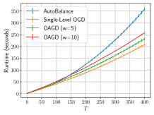
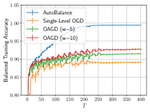
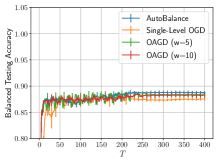
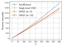
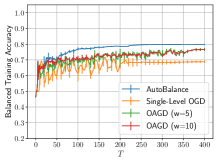
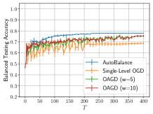
Figure 5 provides a performance comparison (mean$\pm$std) for parametric loss tuning on imbalanced Tadpole data across five runs. We compare our OAGD ($w=5,10$) with AutoBalance and Single-Level OGD. OAGD achieves a comparable balanced testing accuracy to AutoBalance but with a reduced runtime. AutoBalance outperforms OAGD and Single-Level OGD in terms of balanced training accuracy. This is because AutoBalance utilizes many more samples than OAGD and OGD. This allows AutoBalance to have a higher chance of overfitting the training data, resulting in high training accuracy, while still obtaining similar balanced testing accuracy compared to other methods.

Figure 6 provides a performance comparison (mean$\pm$std) on parametric loss tuning for imbalanced Adult data over five runs. We compare our OAGD ($w=5,10$) with AutoBalance and Single-Level OGD. OAGD achieves comparable balanced accuracy to AutoBalance but with a reduced runtime.

D.2 Details and Additional Experiments on Online Meta Learning

This subsection provides the implementation details and additional experiments on miniImageNet of online meta learning.

D.2.1 Datasets and Model Architectures

FC100

FC100 [Oreshkin et al., 2018] is a dataset derived from CIFAR100, containing 100 classes, with each class comprising 600 images of size 32. Following [Oreshkin et al., 2018], the 100 classes are divided as follows: 60 classes for meta-training, 20 classes for meta-validation, and 20 classes for meta-testing. There are 36,000, 12,000, 12,000 samples in the original training, validation and testing datasets, respectively. We transform them into 20,000, 600 and 600 training, validation and testing tasks using the TaskDataset tool from learn2learn [Arnold et al., 2020]. For all comparison algorithms, we employ a 4-layer convolutional neural networks(CNN) comprising four convolutional blocks. Each block consists of a $3\times 3$ convolution (padding=1, stride=2), batch normalization, ReLU activation, and $2\times 2$ max pooling. Additionally, each convolutional layer contains 64 filters.

MiniImageNet

The miniImageNet dataset [Vinyals et al., 2016] is derived from ImageNet and comprises 100 classes, each containing 600 images sized at $84\times 84$. Following the repository, we partition these classes into 64 classes for meta-training, 16 classes for meta-validation, and 20 classes for meta-testing. Following the repository, we use a four-layer CNN with four convolutional blocks, where each block sequentially consists of a $3\times 3$ convolution, batch normalization, ReLU activation, and $2\times 2$ max pooling. Each convolutional layer has 64 filters.

D.2.2 Baselines and Setting Details

In our experiments, we compare our method to three baselines: MAML [Finn et al., 2017], ANIL [Raghu et al., 2019], and ITD-BiO [Ji et al., 2021b]. Notably, these three methods are all implemented using iterative differentiation within the PyTorch framework. They leverage two modules, the features and the head, albeit in distinct ways. The features are used to process the raw input, such as the CNN which processes the image in our case, while the head is responsible for the final classification. To ensure a fair comparison, we set the inner learning rate $\beta=0.1$, the outer learning rate $\alpha$=0.001, and inner step $K=20$ for all the methods.

MAML

MAML stands as the foundational work of meta-learning, in which meta-parameters are learned in the outer loop, while task-specific models are learned in the inner loop using only a small amount of data from the current task. In the implementation, MAML combines features and the head into the meta model, which is then cloned by the local model to perform local adaptation. We update all parameters of the meta model, including those of the features and head.

ANIL

ANIL stands as a widely used meta-learning algorithm that simplifies MAML by eliminating the inner loop for all parts of the MAML-trained network except the task-specific head. In its implementation, only the head of the meta model, cloned by the local model, is employed for subsequent local adaptation. Nonetheless, the features remain utilized for data processing. Ultimately, both the parameters of the features and the head undergo updates.

ITD-BiO

ITD-BiO is a gradient-based stochastic bilevel optimization framework relying on iterative differentiation (ITD). In its implementation, the meta model cloned by the local model comprises solely the head for subsequent local adaptation. Nevertheless, we continue to utilize the features for data processing. Ultimately, only the parameters of the features undergo updates.

It is worth noting that we do not adapt all the baselines to the online environment; instead, we directly utilize the implementation from [Ji et al., 2021b]. In the online environment, data is observed in batches at a time, and the offline method updates the model by incorporating all the data observed up until the current timestep. This will initially speed up the training, but it will progressively slow down over time. Eventually, the entire process will become very time-consuming. Instead, the implementation uses only a fixed number of batches (tasks) randomly sampled from all available tasks at each timestep, which, in our case, is 32. We only use a specific window-size number of batches (tasks) and load them sequentially.

Figure 7: Performance comparison (mean$\pm$std) for online meta-learning on the miniImageNet dataset across five runs. We compare our OAGD ($w=10$) with ANIL and ITD-BiO. OAGD achieves comparable accuracy to the baselines while significantly reducing runtime.

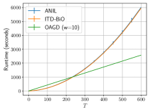
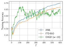
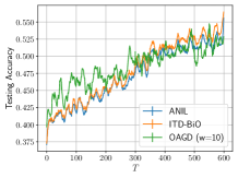
D.2.3 Results on Additional Dataset

We conducted our experiments on an additional dataset, miniImageNet. Figure 7 provides a performance comparison (mean$\pm$std) for meta-learning on the miniImageNet dataset across five runs. We compare our OAGD ($w=10$) with ANIL and ITD-BiO. OAGD achieves comparable accuracy but with a shorter runtime.

D.3 Sensitivity Analysis

Figure 8: Performance comparison (mean$\pm$std) for parametric loss tuning on imbalanced MNIST data across five runs. We compare our OAGD across different window sizes ($w=1,5,10$). The larger the window size, the better the accuracy and the longer the runtime.

Figure 9: Performance comparison (mean$\pm$std) for meta-learning on FC100 data across five runs. We compare our OAGD with different window sizes ($w=1,5,10$). The larger the window size, the better the accuracy and the longer the runtime.

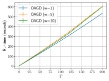
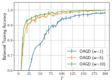
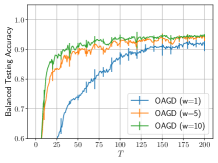
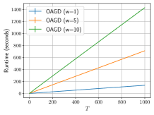
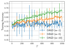
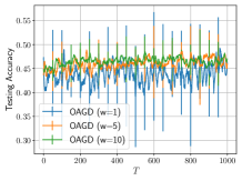
In this section, we perform sensitivity analysis on the window size $w$, learning rate (both inner $\beta$ and outer $\alpha$), and inner optimization step $K$ to acquire a comprehensive understanding of our method.

D.3.1 Sensitivity Analysis of Window Size $w$

Figures 8 and 9 illustrate the results of our OAGD on MNIST and FC100 using different window sizes ($w=1,5,10$). As observed, the larger the window size, the higher the accuracy and the longer the runtime. This is expected, as a larger window size allows for the use of more information from previous timesteps. Consequently, the gradient can be approximated with greater accuracy, leading to improved results. However, this also requires more computations for gradient calculation. It is important to note that we do not merely record previous gradients. Instead, we leverage previous data and the current model to compute the gradients, an approach that has been proven to be more effective.

D.3.2 Sensitivity Analysis of Learning Rates $\alpha$ and $\beta$

Figures 10 and 11 display the sensitivity results for the inner and outer learning rates, $\beta$ and $\alpha$, on the Tadpole dataset. Likewise, Figures 12 and 13 exhibit the sensitivity results for the inner and outer learning rates on the Adult dataset. Specifically, when analyzing the sensitivity to the inner learning rate, we fix the outer learning rate at 0.001 and experiment with different inner learning rates ($\beta=0.9,0.5,0.1,0.01$). Conversely, when examining sensitivity to the outer learning rate, we set the inner learning rate to 0.1 and test different outer learning rates ($\alpha=0.0001,0.001,0.01,0.1$). Our observations indicate that our OAGD is not particularly sensitive to changes in either the inner or outer learning rates, as all cases demonstrate consistently high accuracy.

Figure 10: Performance comparison (mean$\pm$std) on parametric loss tuning for imbalanced Tadpole data over five runs. We compare our OAGD ($w=10$) using various inner learning rates ($\beta=0.01,0.1,0.5,0.9$) while keeping the outer learning rate fixed at $0.001$. Our OAGD is not significantly affected by changes in the inner learning rate.

Figure 11: Performance comparison (mean$\pm$std) on parametric loss tuning for imbalanced Tadpole data over five runs. We compare our OAGD ($w=10$) using various outer learning rates ($\alpha=0.0001,0.001,0.01,0.1$) while maintaining a fixed inner learning rate of $0.1$. Our OAGD is not sensitive to the outer learning rate.

Figure 12: Performance comparison (mean$\pm$std) on parametric loss tuning for imbalanced Adult data over five runs. We compare our OAGD ($w=10$) using various inner learning rates ($\beta=0.01,0.1,0.5,0.9$) while keeping the outer learning rate fixed at $0.001$. Our OAGD is not sensitive to the inner learning rate.

Figure 13: Performance comparison (mean$\pm$std) on parametric loss tuning for imbalanced Adult data across five runs. We compare our OAGD ($w=10$) using different outer learning rates ($\alpha=0.0001,0.001,0.01,0.1$) while keeping the inner learning rate fixed at $0.1$. Our OAGD is not sensitive to the outer learning rate.

Figure 14: Performance comparison (mean$\pm$std) on online meta-learning for miniImageNet data across five runs. We compare our OAGD ($w=10$) with varying inner steps for inner optimization. A larger inner step may yield improved and more stable accuracy but leads to longer runtime.

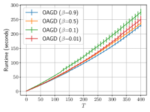
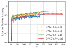
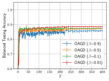
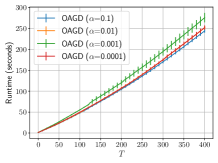
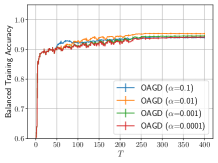
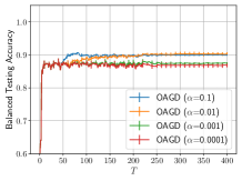
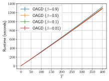
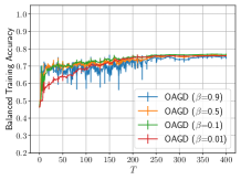
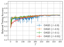
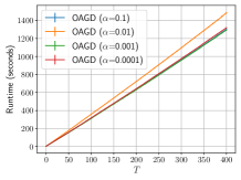
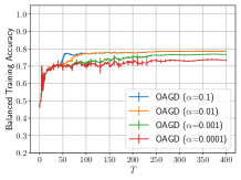
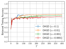
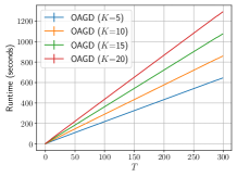
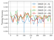
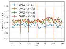
D.3.3 Sensitivity Analysis to Inner Step $K$

Figure 14 provides the sensitivity analysis results to different inner optimization steps $K_{t}=K$ for each round $t$. We can see that a larger inner optimization step can make the accuracy better and more stable. However, this will take longer runtime.

References

- Abernethy et al. [2008] J. Abernethy, P. L. Bartlett, A. Rakhlin, and A. Tewari. Optimal strategies and minimax lower bounds for online convex games. In Proceedings of the 21st Annual Conference on Learning Theory, page 415–423, 2008.
- Agarwal et al. [2019] N. Agarwal, A. Gonen, and E. Hazan. Learning in non-convex games with an optimization oracle. In Conference on Learning Theory, pages 18–29. PMLR, 2019.
- Aiyoshi and Shimizu [1984] E. Aiyoshi and K. Shimizu. A solution method for the static constrained stackelberg problem via penalty method. IEEE Transactions on Automatic Control, 29(12):1111–1114, 1984.
- Al-Khayyal et al. [1992] F. A. Al-Khayyal, R. Horst, and P. M. Pardalos. Global optimization of concave functions subject to quadratic constraints: an application in nonlinear bilevel programming. Annals of Operations Research, 34(1):125–147, 1992.
- Arnold et al. [2020] S. M. Arnold, P. Mahajan, D. Datta, I. Bunner, and K. S. Zarkias. learn2learn: A library for meta-learning research. arXiv preprint arXiv:2008.12284, 2020.
- Aydore et al. [2019] S. Aydore, T. Zhu, and D. P. Foster. Dynamic local regret for non-convex online forecasting. Advances in Neural Information Processing Systems, 32, 2019.
- Baby and Wang [2019] D. Baby and Y.-X. Wang. Online forecasting of total-variation-bounded sequences. In Advances in Neural Information Processing Systems 32, page 11071–11081, 2019.
- Balcan et al. [2019] M.-F. Balcan, M. Khodak, and A. Talwalkar. Provable guarantees for gradient-based meta-learning. In International Conference on Machine Learning, pages 424–433. PMLR, 2019.
- Becker and Kohavi [1996] B. Becker and R. Kohavi. Adult. UCI Machine Learning Repository, 1996. DOI: https://doi.org/10.24432/C5XW20.
- Bertinetto et al. [2018] L. Bertinetto, J. F. Henriques, P. Torr, and A. Vedaldi. Meta-learning with differentiable closed-form solvers. In International Conference on Learning Representations, 2018.
- Besbes et al. [2015] O. Besbes, Y. Gur, and A. Zeevi. Non-stationary stochastic optimization. Operations research, 63(5):1227–1244, 2015.
- Bousquet and Warmuth [2002] O. Bousquet and M. K. Warmuth. Tracking a small set of experts by mixing past posteriors. Journal of Machine Learning Research, 3(Nov):363–396, 2002.
- Bracken and McGill [1973] J. Bracken and J. T. McGill. Mathematical programs with optimization problems in the constraints. Operations Research, 21(1):37–44, 1973.
- Bubeck et al. [2008] S. Bubeck, G. Stoltz, C. Szepesvári, and R. Munos. Online optimization in x-armed bandits. Advances in Neural Information Processing Systems, 21, 2008.
- Chang and Shahrampour [2021] T.-J. Chang and S. Shahrampour. On online optimization: Dynamic regret analysis of strongly convex and smooth problems. In Proceedings of the AAAI Conference on Artificial Intelligence, volume 35, pages 6966–6973, 2021.
- Chen et al. [2021] T. Chen, Y. Sun, and W. Yin. Closing the gap: Tighter analysis of alternating stochastic gradient methods for bilevel problems. Advances in Neural Information Processing Systems, 34, 2021.
- Chen et al. [2022] T. Chen, Y. Sun, and W. Yin. A single-timescale stochastic bilevel optimization method. AISTATS, 2022.
- Chiang et al. [2012] C.-K. Chiang, T. Yang, C.-J. Lee, M. Mahdavi, C.-J. Lu, R. Jin, and S. Zhu. Online optimization with gradual variations. In Conference on Learning Theory, pages 6–1. JMLR Workshop and Conference Proceedings, 2012.
- Daniely et al. [2015] A. Daniely, A. Gonen, and S. Shalev-Shwartz. Strongly adaptive online learning. In International Conference on Machine Learning, pages 1405–1411, 2015.
- Denevi et al. [2019] G. Denevi, D. Stamos, C. Ciliberto, and M. Pontil. Online-within-online meta-learning. Advances in Neural Information Processing Systems, 32, 2019.
- Domke [2012] J. Domke. Generic methods for optimization-based modeling. In Artificial Intelligence and Statistics, pages 318–326. PMLR, 2012.
- Edmunds and Bard [1991] T. A. Edmunds and J. F. Bard. Algorithms for nonlinear bilevel mathematical programs. IEEE transactions on Systems, Man, and Cybernetics, 21(1):83–89, 1991.
- Feurer and Hutter [2019] M. Feurer and F. Hutter. Hyperparameter optimization. In Automated machine learning, pages 3–33. Springer, Cham, 2019.
- Finn et al. [2017] C. Finn, P. Abbeel, and S. Levine. Model-agnostic meta-learning for fast adaptation of deep networks. In International Conference on Machine Learning, pages 1126–1135. PMLR, 2017.
- Finn et al. [2019] C. Finn, A. Rajeswaran, S. Kakade, and S. Levine. Online meta-learning. In International Conference on Machine Learning, pages 1920–1930. PMLR, 2019.
- Franceschi et al. [2017] L. Franceschi, M. Donini, P. Frasconi, and M. Pontil. Forward and reverse gradient-based hyperparameter optimization. In International Conference on Machine Learning, pages 1165–1173. PMLR, 2017.
- Franceschi et al. [2018] L. Franceschi, P. Frasconi, S. Salzo, R. Grazzi, and M. Pontil. Bilevel programming for hyperparameter optimization and meta-learning. In International Conference on Machine Learning, pages 1568–1577. PMLR, 2018.
- Ghadimi and Wang [2018] S. Ghadimi and M. Wang. Approximation methods for bilevel programming. arXiv preprint arXiv:1802.02246, 2018.
- Grazzi et al. [2020] R. Grazzi, L. Franceschi, M. Pontil, and S. Salzo. On the iteration complexity of hypergradient computation. In International Conference on Machine Learning, pages 3748–3758. PMLR, 2020.
- Guo et al. [2021] Z. Guo, Y. Xu, W. Yin, R. Jin, and T. Yang. On stochastic moving-average estimators for non-convex optimization. arXiv preprint arXiv:2104.14840, 2021.
- Hall and Willett [2015] E. C. Hall and R. M. Willett. Online convex optimization in dynamic environments. IEEE Journal of Selected Topics in Signal Processing, 9(4):647–662, 2015.
- Hallak et al. [2021] N. Hallak, P. Mertikopoulos, and V. Cevher. Regret minimization in stochastic non-convex learning via a proximal-gradient approach. In International Conference on Machine Learning, pages 4008–4017. PMLR, 2021.
- Hansen et al. [1992] P. Hansen, B. Jaumard, and G. Savard. New branch-and-bound rules for linear bilevel programming. SIAM Journal on scientific and Statistical Computing, 13(5):1194–1217, 1992.
- Harris et al. [2021] K. Harris, H. Heidari, and S. Z. Wu. Stateful strategic regression. Advances in Neural Information Processing Systems, 34:28728–28741, 2021.
- Hazan [2016a] E. Hazan. Introduction to online convex optimization. Foundations and Trends® in Optimization, 2(3-4):157–325, 2016a. URL http://ocobook.cs.princeton.edu/OCObook.pdf.
- Hazan [2016b] E. Hazan. Introduction to online convex optimization. Foundations and Trends in Optimization, 2(3-4):157–325, 2016b.
- Hazan and Seshadhri [2007] E. Hazan and C. Seshadhri. Adaptive algorithms for online decision problems. In Electronic colloquium on computational complexity (ECCC), volume 14, 2007.
- Hazan et al. [2007] E. Hazan, A. Agarwal, and S. Kale. Logarithmic regret algorithms for online convex optimization. Machine Learning, 69(2):169–192, 2007.
- Hazan et al. [2017] E. Hazan, K. Singh, and C. Zhang. Efficient regret minimization in non-convex games. In International Conference on Machine Learning, pages 1433–1441. PMLR, 2017.
- Héliou et al. [2020] A. Héliou, M. Martin, P. Mertikopoulos, and T. Rahier. Online non-convex optimization with imperfect feedback. Advances in Neural Information Processing Systems, 33:17224–17235, 2020.
- Héliou et al. [2021] A. Héliou, M. Martin, P. Mertikopoulos, and T. Rahier. Zeroth-order non-convex learning via hierarchical dual averaging. In International Conference on Machine Learning, pages 4192–4202. PMLR, 2021.
- Herbster and Warmuth [1998] M. Herbster and M. K. Warmuth. Tracking the best expert. Machine learning, 32(2):151–178, 1998.
- Herbster and Warmuth [2001] M. Herbster and M. K. Warmuth. Tracking the best linear predictor. Journal of Machine Learning Research, 1(281-309):10–1162, 2001.
- Hoi et al. [2021] S. C. Hoi, D. Sahoo, J. Lu, and P. Zhao. Online learning: A comprehensive survey. Neurocomputing, 459:249–289, 2021.
- Hong et al. [2023] M. Hong, H.-T. Wai, Z. Wang, and Z. Yang. A two-timescale stochastic algorithm framework for bilevel optimization: Complexity analysis and application to actor-critic. SIAM Journal on Optimization, 33(1):147–180, 2023.
- Huang and Huang [2021] F. Huang and H. Huang. Biadam: Fast adaptive bilevel optimization methods. arXiv preprint arXiv:2106.11396, 2021.
- Jadbabaie et al. [2015] A. Jadbabaie, A. Rakhlin, S. Shahrampour, and K. Sridharan. Online optimization: Competing with dynamic comparators. In Artificial Intelligence and Statistics, pages 398–406, 2015.
- Ji et al. [2021a] K. Ji, J. Yang, and Y. Liang. Provably faster algorithms for bilevel optimization and applications to meta-learning. In International Conference on Machine Learning, 2021a.
- Ji et al. [2021b] K. Ji, J. Yang, and Y. Liang. Bilevel optimization: Convergence analysis and enhanced design. In International Conference on Machine Learning, pages 4882–4892. PMLR, 2021b.
- Kleinberg et al. [2008] R. Kleinberg, A. Slivkins, and E. Upfal. Multi-armed bandits in metric spaces. In Proceedings of the fortieth annual ACM symposium on Theory of computing, pages 681–690, 2008.
- Krichene et al. [2015] W. Krichene, M. Balandat, C. Tomlin, and A. Bayen. The hedge algorithm on a continuum. In International Conference on Machine Learning, pages 824–832. PMLR, 2015.
- LeCun et al. [2010] Y. LeCun, C. Cortes, and C. Burges. Mnist handwritten digit database. ATT Labs [Online]. Available: http://yann.lecun.com/exdb/mnist, 2, 2010.
- Li et al. [2020] J. Li, B. Gu, and H. Huang. Improved bilevel model: Fast and optimal algorithm with theoretical guarantee. arXiv preprint arXiv:2009.00690, 2020.
- Li et al. [2021] M. Li, X. Zhang, C. Thrampoulidis, J. Chen, and S. Oymak. Autobalance: Optimized loss functions for imbalanced data. Advances in Neural Information Processing Systems, 34:3163–3177, 2021.
- Liang et al. [2023] Y. Liang et al. Lower bounds and accelerated algorithms for bilevel optimization. Journal of Machine Learning Research, 24(22):1–56, 2023.
- Liu et al. [2018] H. Liu, K. Simonyan, and Y. Yang. Darts: Differentiable architecture search. arXiv preprint arXiv:1806.09055, 2018.
- Liu et al. [2020] R. Liu, P. Mu, X. Yuan, S. Zeng, and J. Zhang. A generic first-order algorithmic framework for bi-level programming beyond lower-level singleton. In International Conference on Machine Learning, pages 6305–6315. PMLR, 2020.
- Liu et al. [2021] R. Liu, J. Gao, J. Zhang, D. Meng, and Z. Lin. Investigating bi-level optimization for learning and vision from a unified perspective: A survey and beyond. IEEE Transactions on Pattern Analysis and Machine Intelligence, 44(12):10045–10067, 2021.
- Lv et al. [2007] Y. Lv, T. Hu, G. Wang, and Z. Wan. A penalty function method based on kuhn–tucker condition for solving linear bilevel programming. Applied Mathematics and Computation, 188(1):808–813, 2007.
- Maclaurin et al. [2015] D. Maclaurin, D. Duvenaud, and R. Adams. Gradient-based hyperparameter optimization through reversible learning. In International conference on machine learning, pages 2113–2122. PMLR, 2015.
- Marinescu et al. [2019] R. V. Marinescu, N. P. Oxtoby, A. L. Young, E. E. Bron, A. W. Toga, M. W. Weiner, F. Barkhof, N. C. Fox, P. Golland, S. Klein, et al. Tadpole challenge: Accurate alzheimer’s disease prediction through crowdsourced forecasting of future data. In Predictive Intelligence in Medicine: Second International Workshop, PRIME 2019, Held in Conjunction with MICCAI 2019, Shenzhen, China, October 13, 2019, Proceedings 2, pages 1–10. Springer, 2019.
- Mokhtari et al. [2016] A. Mokhtari, S. Shahrampour, A. Jadbabaie, and A. Ribeiro. Online optimization in dynamic environments: Improved regret rates for strongly convex problems. In 2016 IEEE 55th Conference on Decision and Control (CDC), pages 7195–7201. IEEE, 2016.
- Moore [2010] G. M. Moore. Bilevel programming algorithms for machine learning model selection. Rensselaer Polytechnic Institute, 2010.
- Nazari et al. [2019] P. Nazari, E. Khorram, and D. A. Tarzanagh. Adaptive online distributed optimization in dynamic environments. Optimization Methods and Software, pages 1–25, 2019.
- Nazari et al. [2022] P. Nazari, D. A. Tarzanagh, and G. Michailidis. Dadam: A consensus-based distributed adaptive gradient method for online optimization. IEEE Transactions on Signal Processing, 2022.
- Nesterov [2003] Y. Nesterov. Introductory lectures on convex optimization: A basic course, volume 87. Springer Science & Business Media, 2003.
- Oreshkin et al. [2018] B. Oreshkin, P. Rodríguez López, and A. Lacoste. Tadam: Task dependent adaptive metric for improved few-shot learning. Advances in neural information processing systems, 31, 2018.
- Pedregosa [2016] F. Pedregosa. Hyperparameter optimization with approximate gradient. In International conference on machine learning, pages 737–746. PMLR, 2016.
- Raghu et al. [2019] A. Raghu, M. Raghu, S. Bengio, and O. Vinyals. Rapid learning or feature reuse? towards understanding the effectiveness of maml. arXiv preprint arXiv:1909.09157, 2019.
- Shaban et al. [2019] A. Shaban, C.-A. Cheng, N. Hatch, and B. Boots. Truncated back-propagation for bilevel optimization. In The 22nd International Conference on Artificial Intelligence and Statistics, pages 1723–1732. PMLR, 2019.
- Shalev-Shwartz [2007] S. Shalev-Shwartz. Online learning: Theory, algorithms, and applications. Hebrew University, 2007.
- Shalev-Shwartz et al. [2011] S. Shalev-Shwartz et al. Online learning and online convex optimization. Foundations and trends in Machine Learning, 4(2):107–194, 2011.
- Shi et al. [2005] C. Shi, J. Lu, and G. Zhang. An extended kuhn–tucker approach for linear bilevel programming. Applied Mathematics and Computation, 162(1):51–63, 2005.
- Sinha et al. [2017] A. Sinha, P. Malo, and K. Deb. A review on bilevel optimization: from classical to evolutionary approaches and applications. IEEE Transactions on Evolutionary Computation, 22(2):276–295, 2017.
- Srebro et al. [2010] N. Srebro, K. Sridharan, and A. Tewari. Smoothness, low noise and fast rates. Advances in neural information processing systems, 23, 2010.
- Suggala and Netrapalli [2020] A. S. Suggala and P. Netrapalli. Online non-convex learning: Following the perturbed leader is optimal. In Algorithmic Learning Theory, pages 845–861. PMLR, 2020.
- Sugiyama and Kawanabe [2012] M. Sugiyama and M. Kawanabe. Machine learning in non-stationary environments: Introduction to covariate shift adaptation. MIT press, 2012.
- Vamvoudakis and Lewis [2010] K. G. Vamvoudakis and F. L. Lewis. Online actor–critic algorithm to solve the continuous-time infinite horizon optimal control problem. Automatica, 46(5):878–888, 2010.
- Vinyals et al. [2016] O. Vinyals, C. Blundell, T. Lillicrap, D. Wierstra, et al. Matching networks for one shot learning. Advances in neural information processing systems, 29, 2016.
- von Stackelberg [1952] H. von Stackelberg. Theory of the market economy. United Kingdom: William Hodge, 1952.
- Wei et al. [2016] C.-Y. Wei, Y.-T. Hong, and C.-J. Lu. Tracking the best expert in non-stationary stochastic environments. Advances in neural information processing systems, 29:3972–3980, 2016.
- Wu et al. [2020] Y. F. Wu, W. Zhang, P. Xu, and Q. Gu. A finite-time analysis of two time-scale actor-critic methods. Advances in Neural Information Processing Systems, 33:17617–17628, 2020.
- Yang et al. [2016] T. Yang, L. Zhang, R. Jin, and J. Yi. Tracking slowly moving clairvoyant: Optimal dynamic regret of online learning with true and noisy gradient. In International Conference on Machine Learning, pages 449–457. PMLR, 2016.
- Zhang et al. [2017] L. Zhang, T. Yang, J. Yi, J. Rong, and Z.-H. Zhou. Improved dynamic regret for non-degenerate functions. In NIPS, 2017.
- Zhang et al. [2018a] L. Zhang, S. Lu, and Z.-H. Zhou. Adaptive online learning in dynamic environments. In Advances in neural information processing systems, pages 1323–1333, 2018a.
- Zhang et al. [2018b] L. Zhang, T. Yang, Z.-H. Zhou, et al. Dynamic regret of strongly adaptive methods. In International Conference on Machine Learning, pages 5882–5891, 2018b.
- Zhang et al. [2019] L. Zhang, T.-Y. Liu, and Z.-H. Zhou. Adaptive regret of convex and smooth functions. In International Conference on Machine Learning, pages 7414–7423, 2019.
- Zhang et al. [2020] L. Zhang, S. Lu, and T. Yang. Minimizing dynamic regret and adaptive regret simultaneously. In International Conference on Artificial Intelligence and Statistics, pages 309–319. PMLR, 2020.
- Zhao and Zhang [2021] P. Zhao and L. Zhang. Improved analysis for dynamic regret of strongly convex and smooth functions. In Learning for Dynamics and Control, pages 48–59. PMLR, 2021.
- Zhao et al. [2020] P. Zhao, Y.-J. Zhang, L. Zhang, and Z.-H. Zhou. Dynamic regret of convex and smooth functions. Advances in Neural Information Processing Systems, 33:12510–12520, 2020.
- Zheng et al. [2019] K. Zheng, H. Luo, I. Diakonikolas, and L. Wang. Equipping experts/bandits with long-term memory. Advances in neural information processing systems, 2019.
- Zhou et al. [2020a] W. Zhou, Y. Li, Y. Yang, H. Wang, and T. Hospedales. Online meta-critic learning for off-policy actor-critic methods. Advances in Neural Information Processing Systems, 33:17662–17673, 2020a.
- Zhou et al. [2020b] Y. Zhou, V. Sanches Portella, M. Schmidt, and N. Harvey. Regret bounds without lipschitz continuity: online learning with relative-lipschitz losses. Advances in Neural Information Processing Systems, 33:15823–15833, 2020b.
- Zinkevich [2003] M. Zinkevich. Online convex programming and generalized infinitesimal gradient ascent. In Proceedings of the 20th international conference on machine learning (icml-03), pages 928–936, 2003.