Phase diagram for the TAP energy of the $p$-spin spherical mean field spin glass model

Abstract.

We solve the Thouless-Anderson-Palmer (TAP) variational principle associated to the spherical pure $p$-spin mean field spin glass Hamiltonian and present a detailed phase diagram.

In the high temperature phase the maximum of variational principle is the annealed free energy of the model. In the low temperature phase the maximum, for which we give a formula, is strictly smaller.

The high temperature phase consists of three subphases. (1) In the first phase $m=0$ is the unique relevant TAP maximizer. (2) In the second phase there are exponentially many TAP maximizers, but $m=0$ remains dominant. (3) In the third phase, after the so called dynamic phase transition, $m=0$ is no longer a relevant TAP maximizer, and exponentially many non-zero relevant TAP solutions add up to give the annealed free energy.

Finally in the low temperature phase a subexponential number of TAP maximizers of near-maximal TAP energy dominate.

1. Introduction

In the physics literature on mean field spin glass models such as the Sherrington-Kirkpatrick model the Thouless-Anderson-Palmer (TAP) equations and TAP energy play an important role [TAP77, MPV87, BM80, DY83, GM84, CS92, CHS93, KPV93, CK93, CS95, BBM96, Cav+03]. In mathematics their meaning and implications are an active area of study [Tal10, Section 1.7], [Cha10, Bol14, Sub17, CP18, AJ19, BK19, AJ19a, CPS21, CPS22, Sub20, AJ21, BSZ20, ZSA21, Sub21, BY21, Bel22]. One basic idea is that the TAP energy encodes important information about the free energy and Gibbs measure of the model. In particular, the free energy should be given by a TAP variational principle. In this article we give a detailed phase diagram for the TAP variational principle of the pure $p-$spin spherical spin glass Hamiltonian.

Let $S_{N-1}\subset\mathbb{R}^{N}$ be the $N-1$-dimensional unit sphere and $B_{N}\subset{\mathbb{R}}^{N}$ the $N$-dimensional unit ball. Next for any power series $\xi(x)=\sum_{p\geq 1}a_{p}x^{p}$ with non negative coefficients $a_{p}\geq 0$ satisfying $\xi(1)<\infty$ let the Hamiltonian $H_{N}$ be a centered Gaussian field on $B_{N}$ with covariance

$${\mathbb{E}}[H_{N}(\sigma)H_{N}(\tau)]=N\xi(\sigma\cdot\tau),\quad\sigma,\tau\in B_{N}.$$ (1.1)

The free energy of the model is given by

$$f_{N}\left(\beta\right)=\frac{1}{N}\log\int_{S_{N-1}}\exp\left(\beta H_{N}(\sigma)\right)d\sigma,$$ (1.2)

for an inverse temperature $\beta\geq 0$. As a step towards computing the free energy the TAP energy $H_{\operatorname{TAP}}$ has been introduced (for the standard SK model with $\pm 1$ spins by the eponymous authors in [TAP77], and for the present model with spherical spins in [KPV93]). It is given by

$$H_{\operatorname{TAP}}(m)=\beta H_{N}(m)+\frac{N}{2}\log(1-|m|^{2})+N\operatorname{On}(|m|^{2}),m\in B_{N}^{o},$$ (1.3)

where $B_{N}^{o}$ is the open unit ball in $\mathbb{R}^{n}$ and the third term is the so called Onsager correction

$$\operatorname{On}(q)=\frac{\beta^{2}}{2}\left(\xi(1)-\xi^{\prime}(q)(1-q)-\xi(q)\right).$$ (1.4)

A heuristic derivation of the TAP free energy illustrating the connection with the free energy is given in Section 2. Only the $m$ that satisfy certain conditions are “physical” and relevant for the free energy. In the physics literature it is widely accepted that to be a relevant, $m$ must be a local maximum of $H_{\operatorname{TAP}}$ and it must satisfy Plefka’s condition, which reads $\beta_{2}(|m|^{2})\leq\frac{1}{\sqrt{2}}$, where

$$.\beta_{2}(q)=\beta\sqrt{\frac{\xi^{\prime\prime}(q)}{2}}(1-q).$$ (1.5)

In this paper we replace Plefka’s condition by a slightly stronger condition, namely $|m|^{2}\in D_{\beta}$ where

$$D_{\beta}=\{q\in[0,1]:A(q,\beta)\leq 0\},$$ (1.6)

and

$$A\left(q,\beta\right)=\sup_{r\in\left(0,1\right)}\left(\beta^{2}\frac{\xi^{\prime}\left(q+r\left(1-q\right)\right)(1-q)-\xi^{\prime}\left(q\right)\left(1-q\right)}{r}-\frac{1}{1-r}\right).$$ (1.7)

In Lemma 2.1 we show that $|m|^{2}\in D_{\beta}$ implies that Plefka’s condition $\beta_{2}(|m|^{2})\leq\frac{1}{\sqrt{2}}$ is satisfied. The opposite implication is however not true. Below we further comment on this condition, which is needed to obtain a coherent phase diagram. A critical point of $H_{\operatorname{TAP}}$ is called a TAP solution. We refer to $m$’s which are local maxima of $H_{\operatorname{TAP}}$ that satisfy $|m|^{2}\in D_{\beta}$ as relevant TAP solutions and let the complexity of relevant TAP solutions of a certain energy and certain magnitude be given by the exponential rate

$$I_{\operatorname{TAP}}(U)=\lim_{\varepsilon\downarrow 0}\lim_{N\rightarrow\infty}\frac{1}{N}\log\left|\left\{m\in B^{o}_{N}:\begin{array}[]{c}m\mbox{ loc. max. of }H_{\operatorname{TAP}},|m|^{2}\in D_{\beta}\\ \frac{1}{N}H_{\operatorname{TAP}}(m)\in[U-\varepsilon,U+\varepsilon]\end{array}\right\}\right|\in\{-\infty\}\cup[0,\infty),$$ (1.8)

assuming the limits exist. Defining the total TAP free energy by

$$f_{\operatorname{TAP}}(\beta)=\sup_{U\in\mathbb{R}}\{U+I_{\operatorname{TAP}}(U)\}.$$ (1.9)

a basic idea of the TAP ansatz is the claim that for all $\beta\geq 0$

$$\lim_{N\to\infty}f_{N}(\beta)=f_{\operatorname{TAP}}(\beta).$$ (1.10)

A heuristic argument for this claim is given in Section 2. Combining the present paper with [Sub21] it can be verified “aposteriori” (see below for a more detailed discussion). A direct proof of (1.10) is the subject of active research but is beyond the scope of this paper. However the claim (1.10) motivates the study of the variational principle (1.9), and in this article we do so for the pure $p$-spin models, where

$$\xi(x)=x^{p}\text{ for }p\geq 3.$$ (1.11)

We compute $f_{\operatorname{TAP}}(\beta)$ and $I_{\operatorname{TAP}}$ for all $\beta$, and give a detailed phase diagram characterizing the maximizers for different $\beta$.

We are able to compute the TAP complexity $I_{\operatorname{TAP}}$ since for pure $p$-spin models the Hamiltonian $H_{N}$ is $p$-homogenous and therefore each TAP local maximum in $B_{N}$ corresponds to a local maximum of the Hamiltonian $H_{N}(\sigma)$ on $S_{N-1}$ (in the spherical metric). The complexity of critical points of $H_{N}(\sigma)$ has been determined by [AAČ13, Sub+17]. Their results imply that if $\mathcal{M}(\cdot)$ is the number of local maxima of $H_{N}$ on $S_{N-1}$ with $\frac{H_{N}(\sigma)}{N}\in\cdot$ we have

$$\lim_{\varepsilon\downarrow 0}\lim_{N\to\infty}\frac{1}{N}\log\mathcal{M}([E-\varepsilon,E+\varepsilon])=I\left(E\right)$$ (1.12)

in probability, where $I$ is a function satisfying

$$I\left(E\right)=\begin{cases}>0&\text{if }E\in[E_{\infty},E_{0})\\ 0&\text{ if }E=E_{0}\\ -\infty&\text{ otherwise },\end{cases}$$ (1.13)

for

$$E_{\infty}=\frac{2\sqrt{p-1}}{\sqrt{p}},$$ (1.14)

and where $E_{0}>E_{\infty}$ is the limiting ground state energy of the Hamiltonian $H_{N}$, i.e.

$$\sup_{\sigma\in S_{N-1}}H_{N}(\sigma)=NE_{0}+o(N).$$ (1.15)

The precise definitions of $I$ and $E_{0}$ are given in Section 3.2.

We now state our results for each phase in the phase diagram. The critical temperatures are given in terms of $E_{\infty}$ and $E_{0}$. Our first result shows that the energy surface $H_{\operatorname{TAP}}(m)$ and $I_{\operatorname{TAP}}$ undergoes a phase transition at the complexity threshold $\beta_{c}$. For $\beta<\beta_{c}$ there is only one relevant TAP solution (and even only one TAP solution), namely $m=0$. For $\beta>\beta_{c}$ there are exponentially many relevant TAP solutions. To define $\beta_{c}$ we let

$$\tilde{\beta}_{c}=\frac{1}{2}\sqrt{\frac{p^{p-1}}{(p-1)(p-2)^{p-2}}},$$ (1.16)

as well as

$$\bar{r}=\frac{E_{0}}{E_{\infty}}-\sqrt{\left(\frac{E_{0}}{E_{\infty}}\right)^{2}-1},$$ (1.17)

(note that $\overline{r}<1$) and set

$$\beta_{c}=\bar{r}\tilde{\beta}_{c}.$$ (1.18)

We then have the following.

Theorem 1.1 (Complexity threshold).

For $\beta<\beta_{c}$ there are no relevant TAP solutions except $m=0$, i.e.

$$\lim_{N\to\infty}P\left(m\text{ is a local maximum of }H_{\operatorname{TAP}}\text{ s.t. }|m|^{2}\in D_{\beta}\iff m=0\right)=1.$$ (1.19)

In fact, a fortiori,

$$\lim_{N\to\infty}P\left(m\in B_{N}\text{ is a critical point of }H_{\operatorname{TAP}}\iff m=0\right)=1.$$ (1.20)

In particular

$$I_{\operatorname{TAP}}(U)=\begin{cases}0&\text{ if }U=H_{\operatorname{TAP}}(0)=\frac{\beta^{2}}{2},\\ -\infty&otherwise,\end{cases}$$ (1.21)

and

$$f_{\operatorname{TAP}}(\beta)=\frac{\beta^{2}}{2}.$$ (1.22)

For $\beta>\beta_{c}$ there are exponentially many relevant TAP solutions, i.e.

$$\sup_{U}I_{\operatorname{TAP}}(U)>0.$$ (1.23)

The next theorem describes $I_{\operatorname{TAP}}$ in terms of $I$ when $\beta\geq\beta_{c}$. To formulate the result let

$$\mathcal{N}_{N}(\mathcal{U},\mathcal{V},Q)=\left|\{m\in B_{N}:m\mbox{ loc. max. of }H_{\operatorname{TAP}},\frac{1}{N}H_{\operatorname{TAP}}(m)\in\mathcal{U},\frac{1}{N}H_{N}(m)\in\mathcal{V},|m|^{2}\in Q\}\right|,$$ (1.24)

be the number of TAP solutions with given energy, given energy of the Hamiltonian $H_{N}(m)$ and given squared magnitude and the extended complexity

$$I_{\operatorname{TAP}}(U,V,q)=\lim_{\varepsilon\downarrow 0}\lim_{N\to\infty}\frac{1}{N}\log\mathcal{N}_{N}([U-\varepsilon,U+\varepsilon],[V-\varepsilon,V+\varepsilon],[q-\varepsilon,q+\varepsilon]).$$ (1.25)

That this limit exists is part of our results. Note that

$$I_{\operatorname{TAP}}(U)=\sup_{V\in\mathbb{R},q\in D_{\beta}}I_{\operatorname{TAP}}(U,V,q).$$

For each $V,q$ there can be at most one $U$ such that $I_{\operatorname{TAP}}(U,V,q)\neq-\infty$, since $H_{\operatorname{TAP}}(m)$ is a function of $H_{N}(m)$ and $|m|^{2}$ (see (1.3)). For each $U$ there can in principle be several $(V,q)$ such that $I_{\operatorname{TAP}}(U,V,q)\neq-\infty$, but our analysis implies that this is never the case.

Theorem 1.2.

For $\beta\geq\beta_{c}$ there exist $U_{\min},U_{\max}\in\mathbb{R}$ such that $U_{\min}<U_{\max}\leq\frac{\beta^{2}}{2}$, with equality in the latter inequality only if $\beta=\beta_{d}$, and functions $q_{U}:[U_{\min},\infty)\to D_{\beta}\cap[\frac{p-2}{p},1]$ and $E_{U}:[U_{\min},\infty)\to[E_{\infty},\infty)$ such that

$$I_{{\rm TAP}}\left(U,V,q\right)=\begin{cases}I\left(E\right)&\text{ if }U_{\min}\leq U<U_{\max}\text{ and }q=q_{U}(U),E=E_{U}(U)\\ 0&\text{ if }U=U_{\max}\text{ and }q=q_{U}(U_{\max}),E=E_{U}(U_{\max})\\ 0&\text{\,if }U=\frac{\beta^{2}}{2},V=0,q=0\text{ and }\beta\leq\beta_{d}\\ -\infty&\text{otherwise}.\end{cases}$$

The functions $q_{U},E_{U}$ are strictly increasing, and $E_{U}(U_{\max})=E_{0}$.

A more complete but lengthier specification of $I_{\operatorname{TAP}}$ when $\beta\geq\beta_{c}$ is given in Section 6, and formulas for $U_{\min}$ and $U_{\max}$ are given in Section 7. Note that the theorem implies that when $\beta\geq\beta_{c}$

$$\frac{1}{N}\sup_{m\neq 0\text{ is relevant TAP\ sol.}}H_{\operatorname{TAP}}\left(m\right)\to U_{\max},$$ (1.26)

$$\frac{1}{N}\inf_{m\neq 0\text{ is relevant TAP\ sol.}}H_{\operatorname{TAP}}\left(m\right)\to U_{\min}.$$ (1.27)

We exhibit two further phase transitions of (1.9) at the inverse temperatures

$$\beta_{d}=\sqrt{\frac{(p-1)^{p-1}}{p(p-2)^{p-2}}}$$ (1.28)

corresponding to the dynamic phase transition of the spin glass model and

$$\beta_{s}=\sqrt{\frac{(p-1)^{p-1}}{p\bar{r}^{2}(p-1-\bar{r}^{2})^{p-2}}}$$ (1.29)

which corresponds to the static phase transition. Using $\bar{r}<1$ one can check that indeed

$$\beta_{c}<\tilde{\beta}_{c}<\beta_{d}<\beta_{s}\text{ for all }p\geq 3.$$ (1.30)

To formulate the results we let

$$(U_{*},V_{*},q_{*})=\underset{U\in\mathbb{R},V\in\mathbb{R},q\in D_{\beta}}{\operatorname{argmax}}\left\{U+I_{\operatorname{TAP}}(U,V,q)\right\},$$ (1.31)

when the $\operatorname{argmax}$ is well-defined. When it is well-defined, $U_{*}$ is the maximizer in (1.9), and $q_{*}$ is the squared magnitude and $V_{*}$ the Hamiltonian energy of TAP solutions with energy $U_{*}$. Note that Theorem 1.1 implies that $q_{*}=0$, $V_{*}=0$ and $U_{*}=H_{\operatorname{TAP}}(0)=\frac{\beta^{2}}{2}$ for $\beta<\beta_{c}$. The next theorem shows that while there are exponentially many relevant TAP solutions for $\beta\in(\beta_{c},\beta_{d})$, the behavior of $q_{*},V_{*}$ and $U_{*}$ remains the same up to $\beta_{d}$, i.e. the maximizer in the variational principle (1.9) still corresponds to the relevant TAP solution $m=0$.

Theorem 1.3 (Phase of static and dynamic high temperature).

If $\beta\leq\beta_{d}$ then (1.31) is well defined and

$$\mbox{(a) }q_{*}=0,\quad\mbox{(b) }V_{*}=0\quad\mbox{(c) }U_{*}=H_{\operatorname{TAP}}(0)=\frac{\beta^{2}}{2}>U_{\max}\quad\mbox{(d) }I_{\operatorname{TAP}}(U_{*},V_{*},q_{*})=0,$$ (1.32)

and therefore

$$f_{\operatorname{TAP}}(\beta)=\frac{\beta^{2}}{2}>U_{\max},$$ (1.33)

(where we set $U_{\max}=-\infty$ for $\beta<\beta_{c}$).

For $\beta>\beta_{d}$, we no longer have $0\in D_{\beta}$, so $m=0$ is no longer a relevant TAP solution according to our definition. However our next result shows that in $(\beta_{d},\beta_{s})$, it remains true that $f_{\operatorname{TAP}}(\beta)=\frac{\beta^{2}}{2}$ but this value is achieved in a different way, i.e. $q_{*}$, $V_{*}$, $U_{*}$, $I_{\operatorname{TAP}}(U_{*},V_{*},q_{*})$ are all given by different formulas. Let

$$h_{\operatorname{TAP}}(E,q)=\beta E+\frac{1}{2}\log(1-q)+\operatorname{On}(q),$$ (1.34)

so that

$$H_{\operatorname{TAP}}(m)=\frac{1}{N}h_{\operatorname{TAP}}\left(\frac{H_{N}(m)}{N},|m|^{2}\right).$$ (1.35)

Theorem 1.4 (Phase of dynamic low temperature, static high temperature).

For $\beta\in(\beta_{d},\beta_{s})$ the quantity (1.31) is well defined and it holds that $q_{*}$ is the unique solution of

$$(1-q)q^{p-2}=\frac{1}{p\beta^{2}}\text{ in }\left[\frac{p-2}{p-1},1\right).$$ (1.36)

Furthermore

$$V_{*}=q_{*}^{p/2}E_{*}\text{ for }E_{*}=\frac{E_{\infty}}{2}\left(\frac{1}{\sqrt{2}\beta_{2}(q_{*})}+\sqrt{2}\beta_{2}(q_{*})\right),$$ (1.37)

as well as

$$U_{*}=h_{\operatorname{TAP}}(V_{*},q_{*})$$ (1.38)

hold. Additionally

$$\begin{array}[]{l}I_{\operatorname{TAP}}(U_{*},V_{*},q_{*})=I(E_{*})=-\frac{1}{2}\log(1-q_{*})-\frac{q_{*}}{2}-\frac{q_{*}^{2}}{2p(1-q_{*})}>0\end{array}$$ (1.39)

and

$$f_{\operatorname{TAP}}(\beta)=\frac{\beta^{2}}{2}.$$ (1.40)

Lastly

$$U_{\min}<U_{*}<U_{\max}.$$ (1.41)

The inequality (1.41) shows that $U_{*}$ is not the maximum TAP energy in this phase. Furthermore (1.39) shows that the value of $f_{\operatorname{TAP}}(\beta)$ comes from the contribution of exponentially many relevant TAP solutions $m$ of TAP energy $NU_{*}+o(N)$. This is in contrast to the static low temperature phase we describe next. Indeed after $\beta_{s}$, it is no longer true that $f_{\operatorname{TAP}}(\beta)=\beta^{2}/2$. However once again $I_{\operatorname{TAP}}(U_{\max})=0$, signifying that the maximizer of (1.9) now corresponds to subexponentially many $m$ such that $H_{\operatorname{TAP}}(m)=U_{\max}N+o(N)$ and $H_{N}(m)=E_{0}N+o(N)$. It also gives a formula for $f_{\operatorname{TAP}}(\beta)$, i.e. for the free energy in low temperature.

Theorem 1.5 (Static and dynamic low temperature phase).

For $\beta>\beta_{s}$ we have that (1.31) is well-defined and $q_{*}$ is the unique solution of

$$\beta(1-q)q^{\frac{p-2}{2}}=\frac{\bar{r}}{\sqrt{p(p-1)}}\text{ in }\left[\frac{p-2}{p},1\right).$$ (1.42)

Also

$$\begin{array}[]{lll}\text{(a) }V_{*}=q_{*}^{p/2}E_{0}&\text{(b) }U_{*}=h_{\operatorname{TAP}}(V_{*},q_{*})=U_{\max}&\text{(c) }I_{\operatorname{TAP}}(U_{*},V_{*},q_{*})=0.\end{array}$$ (1.43)

Finally $f_{\operatorname{TAP}}(\beta)$ can be expressed in the various ways

$$\begin{array}[]{ccl}f_{\operatorname{TAP}}(\beta)&=&U_{\max}\\ &=&h_{\operatorname{TAP}}\left(V_{*},q_{*}\right)\\ &=&\displaystyle{\sup_{q\geq\frac{p-2}{p}:\sqrt{2}\beta_{2}(q)\leq 1}}h_{\operatorname{TAP}}(q^{p/2}E_{0},q)\\ &=&\frac{\beta^{2}}{2}+\frac{1}{2}\log\left(1-q_{*}\right)+\frac{2}{p}\frac{q_{*}}{1-q_{*}}\frac{E_{0}}{E_{\infty}}\bar{r}-\frac{1}{2\left(p-1\right)}\left(1+\frac{1}{p}\frac{q_{*}}{1-q_{*}}\right)\frac{q_{*}}{1-q_{*}}\bar{r}^{2}\end{array}$$ (1.44)

and

$$f_{\operatorname{TAP}}(\beta)<\frac{\beta^{2}}{2}.$$ (1.45)

The main points of the above results are summarized in the phase diagram Figure 1. The critical temperatures appearing are summarized in Table 1. All theorems follow from elementary but non-trivial calculations involving the complexity $I$ and the condition (1.6).

Figure 1. Phase diagram of TAP variational principle (1.9), (1.31).
a) TAP free energy $f_{\operatorname{TAP}}(\beta)$ at high and low temperature, see (1.22), (1.33), (1.40), (1.45).
b) Complexity transition, see Theorem 1.1.
c) Whether $m=0$ is relevant TAP solution, see (1.6).
d) Magnitude squared of relevant TAP solutions maximizing TAP variational principle, see (1.32) (a), (1.36), (1.42).
e) Entropy $I_{TAP,*}=I_{\operatorname{TAP}}(U_{*},V_{*},q_{*})$ of relevant TAP solutions maximizing the TAP variational principle, see (1.32) (c), (1.39), (1.43) (c).

Notation	Formula	Value ($p=3$)	Description
$\beta_{c}$	$\tilde{\beta}_{c}\bar{r}$	0.89372	Complexity transition
$\tilde{\beta}_{c}$	$\frac{1}{2}\sqrt{\frac{p^{p-1}}{(p-1)(p-2)^{p-2}}}$	1.06066	TAP loc. max. start existing $\forall$ $E\in[E_{\infty},E_{0}]$
$\beta_{d}$	$\sqrt{\frac{(p-1)^{p-1}}{p(p-2)^{p-2}}}$	1.15470	Dynamical phase transition
$\beta_{s}$	$\sqrt{\frac{(p-1)^{p-1}}{p\bar{r}^{2}(p-1-\bar{r}^{2})^{p-2}}}$	1.20656	Static phase transition

Table 1. Critical temperatures; $\bar{r}$ is defined in (1.17). The description for $\tilde{\beta}_{c}$ is explained in Remark 6.2.

1.1. The condition $|m|^{2}\in D_{\beta}$

The condition is motivated by the heuristic argument behind (1.10) and a replica computation from [CL06]. It is further explained in Section 2. As mentioned above the condition $A(q,\beta)\leq 0$ is stronger than Plefka’s condition. However, at least for pure $p$-spin models it is only slightly stronger, in that it ultimately only additionally determines when the local maximum $m=0$ should be considered relevant; with high probability there are no other local maxima where $A(q,\beta)\leq 0$ is satisfied and Plefka’s condition is not, see Theorem 2.2 for more details. The stronger condition is necessary to get a coherent phase diagram. For instance if only Plefka’s condition is required for a TAP local maximum to be $m$ considered relevant, the claim (1.10) can not be true, since $m=0$ always satisfies Plefka’s condition and would always be a relevant TAP solution and we would have $f_{\operatorname{TAP}}(\beta)\geq\frac{\beta^{2}}{2}$ for all $\beta\geq 0$.

1.2. Relation to [Sub21, AJ21]

While preparing the current article the two related works [Sub21, AJ21] appeared.

The article [Sub21] computes the limit $N\to\infty$ of the free energy (1.2) of the spherical models considered in the paper for all $\beta$ using a TAP approach, though one involving limiting properties of the Gibbs measure via the concept of “multisamplable overlap” which is therefore different from TAP approach envisioned in the heuristic in Section 2. In the framework of [Sub21] only the ground state energy $E_{0}$ of $H_{N}$ plays a role, rather than the full TAP complexity. Therefore the phase transitions $\beta_{c}$ and $\beta_{d}$ can not be detected in that framework. The phase transition $\beta_{s}$ can however be detected, and [Sub21] presents a formula for it which is different but can be shown to be equivalent to the the formula (1.29) in the paper (see [Sub21, (1.9)-(1.10)]). It also presents the formula $h_{\rm{TAP}}(V_{*},q_{*})$ which we also derive in this paper (see (1.44) and [Sub21, (1.11)-(12)]). In contrast to the present paper, which only deals with the variational principle (1.9), the paper [Sub21] computes the limiting free energy. It proves that for $\beta\leq\beta_{s}$ it holds that $\lim_{N\to\infty}f_{N}(\beta)=\frac{\beta^{2}}{2}$ and for $\beta\geq\beta_{s}$ one has $\lim_{N\to\infty}f_{N}(\beta)=h_{\rm{TAP}}(V_{*},q_{*})$, where $V_{*},q_{*}$ are as in Theorem 1.5. Since Theorems 1.1-1.4 show that $f_{\operatorname{TAP}}(\beta)=\frac{\beta^{2}}{2}$ for $\beta\leq\beta_{s}$ and Theorem 1.5 shows that $f_{\operatorname{TAP}}(\beta)=h_{\rm{TAP}}(V_{*},q_{*})$ we can “aposteriori” conclude that (1.10) is indeed true. However, in the TAP approach envisioned by [BK19, Bel22] and the present work one wishes to prove this rather by obtaining a direct microcanonical proof of (1.10), which would then yield an alternative proof of the results for the limiting free energy of [Sub20] when combined with the present paper.

The “TAP decomposition” of [AJ21] is more similar to the TAP approach envisioned here, and here the analysis is sensitive to the threshold $\beta_{d}$. Indeed [AJ21, Theorems 2.1, 2.4] proves that there is a $\delta>0$ such that for $\beta\in(\beta_{d}-\delta,\beta_{d})$ the free energy can be lower bounded by the contribution of exponentially many “slices” around TAP solutions, giving a total contribution of $\beta^{2}/2$ (cf. Section 2 and Theorem 1.4). A similar computation of the free energy for large enough $\beta$ was carried out in [Sub17]. This is the kind of analysis that the authors hope to in the future extend to all $\beta$, whereby the aim is to separate the analysis neatly into a proof of (1.10) for all $\beta$ (a first step has been taken in [Bel22]) and an analysis of variational principle (1.9) for all $\beta$, which is provided by the present paper.

1.3. Further results and structure of paper

Sections 4, 6 and 7 contain further results that are of independent interest beyond their role as intermediate steps in the proofs of Theorem 1.1-1.5. Theorem 4.4 of Section 4 gives various results that deterministically relate TAP energy $H_{\operatorname{TAP}}(m)$, Hamiltonian energy $H_{N}\left(\frac{m}{|m|}\right)$ and magnitude $|m|^{2}$ for any relevant TAP solution, and that follow purely from the conditions $|m|^{2}\in D_{\beta}$ and that a relevant TAP solution must be a local maximum. Theorem 6.1 of Section 6 gives a more detailed version of Theorem 1.2. Proposition 7.1 gives formulas for $U_{\min}$ and $U_{\max}$. Theorems 1.3-1.5 are proved in Section 8. In Section 2 we give a heuristic behind (1.10) and the condition (1.6). Section 3 recalls some known facts about $H_{N}$, including the full definition of the complexity $I$ and $E_{0}$, that we use in this paper.

Table 2 contains a list of notation used in this paper.

Notation	Description	Definition
$H_{N}(m)$	Hamiltonian energy	(1.1)
$H_{\operatorname{TAP}}(m)$	TAP energy as function of $m$	(1.3)
$h_{\operatorname{TAP}}(E,|m|^{2})$	TAP energy as function of Hamiltonian energy $E=H_{N}(m)$ and $|m|^{2}$	(1.34)
$E_{0},E_{\infty}$	Largest and smallest energies of $p$-spin Hamiltonian local maxima	(1.14) and (3.7)
$\beta_{2}(q)$	Quantity appearing in Plefka’s condition	(1.5)
$\xi(x)=x^{p}$	Covariance function of $p$-spin Hamiltonian	(1.11)
$\operatorname{On}(q)$	Onsager correction	(1.4)
$f(E,q)$	$h_{\operatorname{TAP}}(q^{p/2}E,q)$	(4.3)
$D_{\beta},A(q,\beta)$	$D_{\beta}=\{q:A(q,\beta)\leq 0\}$ set of possible squared radii of relevant TAP solutions	(1.6), (1.7)
$U_{\max},U_{\min}$	Largest and smallest TAP energies of nonzero relevant TAP  solutions	(4.39), (6.3)
$V_{*},U_{*},q_{*}$	Energy, $\operatorname{TAP}$ energy and squared radius with largest contribution to relevant TAP free energy	(1.31)
$E_{q},q_{E}$	Energy of nonzero relevant TAP  solution of given squared radius, and squared radius of nonzero relevant TAP solution of given energy	(4.31), (4.33)
$E_{U},q_{U}$	Energy, squared radius of nonzero relevant TAP  solution for given $\operatorname{TAP}$ energy	(4.42), (6.7)
$I_{\operatorname{TAP}}(U,V,q)$	Entropy of relevant TAP local maxima of TAP energy	(1.25)
$E_{\min},q_{\min}$	Minimal energy on unit sphere of nonzero relevant TAP solutions and corresponding squared radius	(4.25), (4.27)
$r_{\pm}\left(\frac{E}{E_{\infty}}\right)$	Solutions of $\frac{E}{E_{\infty}}=\frac{1}{2}(\frac{1}{x}+x)$ with $r_{-}\left(\frac{E}{E_{\infty}}\right)\leq 1\leq r_{+}\left(\frac{E}{E_{\infty}}\right)$	(4.6)
$\bar{r}$	$r_{-}(\frac{E_{0}}{E_{\infty}})$	(1.17)
$\mathcal{N}_{N}$	Number of relevant TAP solutions with TAP energy, Hamiltonian energy and squared radius in given sets	(1.24)

Table 2. Index of notation

2. Heuristic derivation of the relevant TAP variational principle

In this section we give a heuristic derivation of the TAP energy (1.3) and (1.10). It is an adaptation of the heuristic that has been turned into a proof of (1.10) in the special case $p=2$ in [BK19], and an upper bound for the free energy in terms of the TAP energy in [Bel22]. The heuristic also motivates the condition (1.6).

The starting point is that in high temperature and without external field the free energy of a Hamiltonian $H_{N}$ whose covariance is given by $\xi$ takes a simple form

$$Z_{N}=e^{N\frac{\beta^{2}}{2}\xi(1)+o\left(N\right)}.$$ (2.1)

The estimate (2.1) of course does not hold in low temperature. In this heuristic we make the ansatz that (2.1) is true at least in the region reported in [CL06] as featuring stability in the replica computation. Their condition can be written as

$$\sup_{r\in[0,1]}\left(\beta^{2}\frac{\xi^{\prime}(q)}{r}-\frac{1}{1-r}\right)\geq 0.$$ (2.2)

To argue heuristically that in low temperature the free energy can be written in terms of the TAP energy, we first lower bound the partition function by the integral of the Gibbs factor over a “slice” $A_{\varepsilon}=\left\{\sigma\in S:\left|\left(\sigma-m\right)\cdot m\right|\leq\varepsilon\right\}$ for some $m\in B$:

$$Z_{N}\geq\int_{A_{\varepsilon}}e^{\beta H_{N}\left(\sigma\right)}E(d\sigma).$$ (2.3)

The set $A_{\varepsilon}$ is an $\varepsilon$-thickened version of the intersection $A_{0}$ of the hyperplane perpendicular to $m$ passing through $m$, and the sphere. The set $A_{0}$ is precisely a $N-2$-dimensional sphere of radius $\sqrt{1-|m|^{2}}$ which has surface area $(1-|m|)^{\frac{N}{2}+o(N)}$. For $\varepsilon\downarrow 0$ slow enough with $N$. The measure of $A_{\varepsilon}$ under $E$ is also $(1-|m|)^{\frac{N}{2}+o(N)}$.

After normalization the integral in (2.3) it can be approximated by an uniform integral on $A_{0}$, giving that

$$Z_{N}\geq\exp\left(\frac{N}{2}\log(1-|m|^{2})+o(N)\right)\int_{A_{0}}e^{\beta H_{N}\left(\sigma\right)}d\sigma,$$ (2.4)

where the integral is now against the uniform measure on $A_{0}$.

Inside the slice $A_{0}$, it is natural to expand the Hamiltonian in $\hat{\sigma}=\sigma-m$ giving

$$H_{N}\left(m+\hat{\sigma}\right)=H_{N}\left(m\right)+\nabla H_{N}\left(m\right)\cdot\hat{\sigma}+H_{N}^{m}\left(\hat{\sigma}\right),$$ (2.5)

where $H_{N}^{m}\left(\hat{\sigma}\right)$ collects all the terms of order $2$ or higher in the $\hat{\sigma}_{i}$. One can show that for fixed $m$

$$H_{N}\left(m\right),\left(\nabla H_{N}\left(m\right)\cdot\hat{\sigma}\right)_{\hat{\sigma}:\hat{\sigma}\cdot m=0},\left(H_{N}^{m}\left(\hat{\sigma}\right)\right)_{\hat{\sigma}:\hat{\sigma}\cdot m=0},$$

are independent, and that $H_{N}^{m}\left(\hat{\sigma}\right)$ is a mixed $p$-spin Hamiltonian on the $N-2$-dimensional sphere $\left\{\hat{\sigma}:\hat{\sigma}\cdot m=0\right\}$ with covariance

$$\mathbb{E}\left[H_{N}^{m}\left(\hat{\sigma}\right)H_{N}^{m}\left(\hat{\sigma}^{\prime}\right)\right]=\xi^{|m|^{2}}(\hat{\sigma}\cdot\hat{\sigma}^{\prime}),$$

where

$$\xi^{q}\left(x\right)=\xi\left(q+x\left(1-q\right)\right)-\xi^{\prime}\left(q\right)x\left(1-q\right)-\xi\left(q\right),$$

(see Lemma 3.2 [Bel22]). With (2.5) the integral in (2.4) can be written as

$$e^{\beta H_{N}(m)}\int_{A_{0}}e^{\beta\nabla H_{N}\left(m\right)\cdot\hat{\sigma}+\beta H_{N}\left(\hat{\sigma}\right)}d\sigma.$$ (2.6)

This integral reveals itself as the partition function of a spherical model on $A_{0}$ with external field $\beta\nabla H_{N}\left(m\right)$ and Hamiltonian $H_{N}^{m}\left(\hat{\sigma}\right)$. Rewriting in this way is useful if we can expect this integral to be estimated in a simpler way than the original one, by a simpler expression. If the external field field vanishes, and if $\beta$ is small enough depending on the covariance $\xi^{m}$ then the expression (2.1) gives such a simple expression. We therefore restrict our attention only to $m$:s such that $\nabla H_{N}\left(m\right)\propto m$ so that the partition function on the bottom line of (2.6) has no external field, and the covariance $\xi^{|m|^{2}}$ of the slice satisfies (2.2). The covariance $\xi^{|m|^{2}}$ satisfies (2.2) precisely if (1.6) holds; this is the motivation for (1.6). When this is the case we can heuristically use (2.1) on the partition function in (2.6) and we obtain that (2.6) should equal

$$e^{\beta H_{N}(m)+\frac{\beta^{2}}{2}\xi_{q}(1)},$$

for any fixed $m$ such that (1.6) and $\nabla H_{N}(m)\propto m$ are satisfied. For such $m$ , it would follow from (2.6) that

$$Z_{N}\geq e^{\beta H_{N}(m)+\frac{N}{2}\log(1-|m|^{2})+\frac{\beta^{2}}{2}\xi_{q}(1)}=e^{H_{\operatorname{TAP}}(m)+o(N)}.$$ (2.7)

Thus we have heuristically arrived at the formula (1.3) for the TAP energy.

To obtain the best possible lower bound, it is natural to maximize $H_{\operatorname{TAP}}(m)$, leading one to consider $m$ that are maximizers of $H_{\operatorname{TAP}}(m)$. These will be critical points of $H_{\operatorname{TAP}}(m)$, which because of the spherical symmetry of all terms in $H_{\operatorname{TAP}}$ except $H_{N}(m)$ means that $m$ will be a critical point of $H_{N}$ in the spherical metric, which incidentally is equivalent to the condition $\nabla{H_{N}}(m)\propto m$ assumed above to find a heuristic lower bound for the partition function. Thus, heuristically, we arrive at the lower bound

$$\begin{array}[]{ccl}Z_{N}\geq e^{H_{\operatorname{TAP}}(m)+o(N)}\text{ for any local maximum $m$ of $H_{\operatorname{TAP}}$ satisfying \eqref{eq: our plefka}}.\end{array}$$ (2.8)

If there are many local maxima, it is natural that these need to be added up to give the true magnitude of $Z_{N}$. Assuming that any over-counting arising in this way causes only lower order errors, we heuristically arrive at the estimate

$$Z_{N}=\sum_{m:\text{ loc max of }H_{\operatorname{TAP}},|m|^{2}\in D_{\beta}}e^{H_{\operatorname{TAP}}(m)+o(N)}.$$

Since

$$\lim_{N\to\infty}\frac{1}{N}\log\left(\sum_{m:\text{ loc max of }H_{\operatorname{TAP}},|m|^{2}\in D_{\beta}}e^{H_{\operatorname{TAP}}(m)+o(N)}\right)=f_{\operatorname{TAP}}(\beta),$$

we arrive heuristically at (1.10).

One can show that (2.2) is equivalent to $\beta<\beta_{d}$ when $\xi(x)=x^{p}$, so that if (1.10) is true, then it follows from Theorem 1.4 that the estimate (2.1) in fact remains true also for a range of $\beta$ that do not satisfy (2.2), but for a very different reason, as comparing Theorems 1.3 and 1.4 shows.

Proving that (2.2) indeed implies (2.1) is the subject of active research and beyond the scope of the present article. A direct rigorous proof of such an implication will likely combine with the theorems of this paper to yield a fully rigorous computation of the free energy via a TAP approach. The condition (2.2) arises from a replica calculation. It is possible that a different method would lead to a different, but ultimately equivalent condition. We hope that future work will find a direct proof of (2.2) that gives rise to a such a condition. It is also possible that a non-equivalent condition is obtained. However, in the proofs of the present article we only use the following properties of the set $D_{\beta}$.

Lemma 2.1.

The family of sets $(D_{\beta})_{\beta\geq 0}$ in (1.6) satisfies

1. $D_{\beta}\cap\left[\frac{p-2}{p},1\right]=\left\{q\in\left[\frac{p-2}{p},1\right]:\beta_{2}(q)\leq\frac{1}{\sqrt{2}}\right\}.$

2. $D_{\beta}\cap\left[0,\frac{p-2}{p}\right)\subset\left\{q\in\left[0,\frac{p-2}{p}\right):\beta_{2}(q)\leq\frac{1}{\sqrt{2}}\right\}$.

3. $0\in D_{\beta}\iff\beta\leq\beta_{d}$.

As these are the only properties of $D_{\beta}$ used, all our results will remain true if our condition is replaced by any other condition also satisfying these properties:

Theorem 2.2.

If $(D_{\beta})_{\beta\geq 0}$ in (1.6) is replaced by any collection of sets indexed by $\beta$ that satisfy Lemma 2.1 1), 2) and 3) then all the results stated in the introduction remain true. In fact everything except the proof of Lemma 2.1 remains exactly the same.

2.1. Relation between conditions

In this section we prove the properties of $D_{\beta}$ stated in Lemma 2.1, that are needed for the analysis in this paper. Before stating the results we recall (1.6) and (1.7) which state that $D_{\beta}=\{q\in[0,1]:A(q,\beta)\leq 0\}$, where

$$A\left(q,\beta\right)=\sup_{r\in\left(0,1\right)}\left(\beta^{2}\frac{\xi^{\prime}\left(q+r\left(1-q\right)\right)(1-q)-\xi^{\prime}\left(q\right)\left(1-q\right)}{r}-\frac{1}{1-r}\right).$$ (2.9)

Prof of Lemma 2.1 1) 2).

We first show that for $q\in[0,1]$, $\beta\geq 0$ we have

$$A(q,\beta)\leq 0\Rightarrow\beta_{2}(q)\leq\frac{1}{\sqrt{2}}.$$ (2.10)

Let $A(q,\beta)\leq 0$. Then by the definition of (2.9) of $A$

$$0\geq\lim_{r\searrow 0}\left(\beta^{2}(1-q)\frac{\xi^{\prime}(q+r(1-q))-\xi^{\prime}(q)}{r}-\frac{1}{1-r}\right)=\beta^{2}(1-q)^{2}\xi^{\prime\prime}(q)-1\overset{\eqref{eq: beta2 def}}{=}2\beta_{2}(q)^{2}-1,$$

so (2.10) follows. This proves Lemma 2.1 2).

Next we show for $q\geq\frac{p-2}{p}$, $\beta\geq 0$, that we have

$$\beta_{2}(q)\leq\frac{1}{\sqrt{2}}\Rightarrow A(q,\beta)\leq 0,$$ (2.11)

which together with (2.10) also implies Lemma 2.1 1). Since $\xi^{\prime}\left(x\right)=px^{p-1}$ we have using the definition (1.5) of $\beta_{2}$ that

$$\beta^{2}\left(1-q\right)\frac{\xi^{\prime}\left(q+r\left(1-q\right)\right)-\xi^{\prime}\left(q\right)}{r}=2\beta_{2}\left(q\right)^{2}\frac{\left(1+r\frac{1-q}{q}\right)^{p-1}-1}{\left(p-1\right)r\frac{1-q}{q}}.$$ (2.12)

Consider

$$\frac{\left(1+r\frac{1-q}{q}\right)^{p-1}-1}{\left(p-1\right)r\frac{1-q}{q}}.$$ (2.13)

By the binomial theorem the left-hand equals

$$\frac{1}{p-1}\sum_{k=0}^{p-2}{{p-1}\choose{k+1}}\left(r\frac{1-q}{q}\right)^{k}.$$

Now if $q\geq\frac{p-2}{p}$ then $\frac{1-q}{q}\leq\frac{2}{p-2}$ so that this is at most

$$\frac{1}{p-1}\sum_{k=0}^{p-2}{p-1\choose k+1}\left(\frac{2}{p-2}\right)^{k}r^{k}.$$

Using the inequalities ${p-1\choose k+1}\leq\frac{\left(p-1\right)\left(p-2\right)^{k}}{\left(k+1\right)!}$ and $\frac{2^{k}}{\left(k+1\right)!}\leq 1$ we get that this is at most $\sum_{k=0}^{p-2}r^{k}\leq\frac{1}{1-r}$. We thus have for all $q\geq\frac{p-2}{p}$ and $r\in\left[0,1\right]$ that

$$\frac{\left(1+r\frac{1-q}{q}\right)^{p-1}-1}{\left(p-1\right)r\frac{1-q}{q}}\leq\frac{1}{1-r}.$$ (2.14)

Combining this with (2.12) we obtain that $A\left(q,\beta\right)\leq 0$ when $2\beta_{2}\left(q\right)^{2}\leq 1$.

∎

Proof of Lemma 2.1 3).

We show that

$$A(0,\beta)\leq 0\Leftrightarrow\beta\leq\beta_{d}.$$

By definition (2.9) of $A$ the expression $A(0,\beta)\leq 0$ reads

$$\sup_{r\in\left(0,1\right)}\left(\beta^{2}\frac{\xi^{\prime}\left(r\right)}{r}-\frac{1}{1-r}\right)\leq 0.$$

Since $\xi^{\prime}(x)=px^{p-1}$ this is equivalent to

$$\sup_{r\in(0,1)}\left(r^{p-2}(1-r)\right)\leq\frac{1}{p\beta^{2}}.$$

The left hand side is easily checked to be maximized at $r=\frac{p-2}{p-1}$. Thus $A(0,\beta)\leq 0$ is equivalent to

$$\frac{(p-2)^{p-2}}{(p-1)^{p-1}}\leq\frac{1}{p\beta^{2}},$$

which is equivalent to $\beta\leq\beta_{d}$ by the definition (1.28) of $\beta_{d}$.

∎

3. Preliminaries

3.1. Hamiltonian as random homogeneous polynomial

We record the standard fact that the Hamiltonian in (1.1) with $\xi(x)=x^{p},p\geq 1,$ can be explicitly constructed by letting

$$H_{N}(\sigma)=\sqrt{N}\sum_{i_{1},\ldots,i_{p}=1}^{N}J_{i_{1},\ldots,i_{p}}\sigma_{i_{1}}\ldots\sigma_{i_{p}},\sigma\in\mathbb{R}^{N},$$ (3.1)

where $J_{i_{1},\ldots,i_{p}}$ are independent standard Gaussians. This implies that $H_{N}(\sigma)$ is almost surely $p$-homogenous, which will be crucial.

3.2. Critical point complexity of Hamiltonian

In this subsection we recall the precise form of the critical point complexity for pure $p$-spin models. Let

$$\mathcal{C}_{N}(A)=\frac{1}{N}\log|\{\sigma\in S_{N-1}:\nabla_{\rm{sp}}H_{N}(\sigma)=0,\frac{1}{N}H_{N}(\sigma)\in A\}|,$$

where $\nabla_{\rm{sp}}$ denotes the spherical gradient, be the number of critical points of $H_{N}$ in the spherical metric with scaled energy in the set $A$, and let

$$\mathcal{M}_{N}(A)=\frac{1}{N}\log|\{\sigma\in S_{N-1}:\nabla_{\rm{sp}}H_{N}(\sigma)=0,m\text{ is loc. max.},\frac{1}{N}H_{N}(\sigma)\in A\}|,$$

be the same for local maxima. Let the log potential of the semi-circle law $\mu_{sc}$ (with support on $[-1,1]$) be denoted by

$$\Omega(\eta)=\int\log|\eta-x|\mu_{sc}(dx)=\eta^{2}-\frac{1}{2}-\eta\sqrt{\eta^{2}-1}+\log(\eta+\sqrt{\eta^{2}-1}),$$ (3.2)

for $\eta\geq 1$. Also let

$$g\left(\eta\right)=\begin{cases}-\infty&\text{ if }\eta<1,\\ \frac{1}{2}+\frac{1}{2}\log(p-1)-2\frac{p-1}{p}\eta^{2}+\Omega(\eta)&\text{ if }\eta\geq 1.\end{cases}$$ (3.3)

Then the annealed complexity is given by the function

$$I_{\rm{Ann}}\left(E\right)=g\left(\frac{E}{E_{\infty}}\right),$$ (3.4)

and the quenched by

$$I\left(E\right)=\begin{cases}g\left(\frac{E}{E_{\infty}}\right)&\text{\,if }g\left(\frac{E}{E_{\infty}}\right)\geq 0,\\ -\infty&\text{if }g\left(\frac{E}{E_{\infty}}\right)<0,\end{cases}$$ (3.5)

One can verify that

$$I_{\operatorname{Ann}}(E)\text{ is strictly decreasing on }[E_{\infty},\infty),$$ (3.6)

and using the notation of [AAČ13] one

$$\text{denotes by }E_{0}\text{ the unique zero of }I_{\operatorname{Ann}}\text{ in }[E_{\infty},\infty),$$ (3.7)

so that

$$I\left(E\right)=\begin{cases}g\left(\frac{E}{E_{\infty}}\right)>0&\text{ for }E\in[E_{\infty},E_{0}),\\ 0&\text{ for }E=E_{0},\\ -\infty&\text{\,for }E\notin\left[E_{\infty},E_{0}\right],\end{cases}$$ (3.8)

We have the following.

Theorem 3.1 ([AAČ13], [Sub+17]).

For all $E$

$$\lim_{\varepsilon\downarrow 0}\lim_{N\to\infty}\mathcal{C}_{N}([E-\delta,E+\delta])=I(E),$$

where the convergence is in probability.

Note that Theorem 3.1 and (3.8) imply (1.15).

From Theorem 3.1 one easily derives the equivalent result for local maxima.

Corollary 3.2.

For all $E$

$$\lim_{\varepsilon\downarrow 0}\lim_{N\to\infty}\mathcal{M}_{N}([E-\delta,E+\delta])=I(E),$$

where the convergence is in probability.

Proof.

Let $\mathcal{C}([E,\infty))$ denote the number of all critical points of $H_{N}\left(\sigma\right)$ on $S_{N-1}$ with $\frac{H_{N}\left(\sigma\right)}{N}\in[E,\infty)$, and let $\mathcal{M}\left(\left[E,\infty\right)\right)\leq\mathcal{C}\left(\left[E,\infty\right)\right)$ denote the number of local maxima satisfying the same condition. Theorems 2.5 and 2.8 [AAČ13] show that

$$\lim_{N\to\infty}\frac{1}{N}\log\mathbb{E}\left[\mathcal{C}([E,\infty))\right]=\lim_{N\to\infty}\frac{1}{N}\log\mathbb{E}\left[\mathcal{M}([E,\infty))\right]=g\left(\frac{E}{E_{\infty}}\right)\text{ for all }E\geq E_{\infty},$$

for $g$ given by (3.3) (cf. (2.15)-(2.16) of [AAČ13]; the results of [AAČ13] and [Sub+17] are stated for negative energies and local minima, since $H_{N}\overset{law}{=}-H_{N}$ the equivalent results for local maxima stated here and below follow). Since $\mathcal{M}([E,\infty))$ is an integer it follows by Markov’s inequality that

$$\lim_{N\to\infty}\frac{1}{N}\log\mathcal{C}([E,\infty))=\lim_{N\to\infty}\frac{1}{N}\log\mathcal{M}([E,\infty))=-\infty\text{\,for }E\geq E_{0},$$

for $E_{0}$ defined below (1.12), where the limits are in probability. Corollary 2 of [Sub+17] implies that

$$\lim_{N\to\infty}\frac{1}{N}\log\mathcal{C}([E,\infty))=I\left(E\right)\text{\,for }E\in\left(E_{\infty},E_{0}\right).$$ (3.9)

Theorem 2.5 [AAČ13] shows that for any fixed $k\geq 1$ the number of critical points of index $k$ is much smaller than $e^{NI(E)}$, strongly suggesting that (3.11) below follows. To also cover the case of diverging $k$ we invoke Theorem 2.15 [AAČ13] and the fact that $E_{k}$ ($E_{k}(3)$ in the notation of [AAČ13]) satisfies $\lim_{k\to\infty}E_{k}=E_{\infty}$. The latter shows that for any $E>E_{\infty}$ there is a $K$ such that $E>E_{K}$. Then using Theorem 2.5 [AAČ13] for critical points of index $1,\ldots,K$ and Theorem 2.15 [AAČ13] for indices larger than $K$ we get

$$\lim_{N\to\infty}\frac{1}{N}\log\left(\mathcal{C}([E,\infty))-\mathcal{M}([E,\infty))\right)\leq I(E)-I_{1}(E),$$ (3.10)

for $I_{1}$ as in (2.14) of [AAČ13], which is positive for all $E\in\left(E_{\infty},E_{0}\right)$. From (3.9) and (3.10) it follows that in fact

$$\lim_{N\to\infty}\frac{1}{N}\log\mathcal{M}([E,\infty))=I\left(E\right)\text{\,for }E\in\left(E_{\infty},E_{0}\right).$$ (3.11)

Since $I\left(E\right)$ is strictly decreasing for $E\in\left(E_{\infty},E_{0}\right)$ the claim (1.12) follows. ∎

4. Deterministic characterization of relevant TAP solutions

In this section we derive a characterization of relevant TAP solutions that arises determinstically from the condition that $m$ must be a local maximum of $H_{\operatorname{TAP}}$ and satisfy $|m|^{2}\in D_{\beta}$, together with two basic deterministic properties of $H_{N}$ (namely (4.1) below). We will make no reference to the random behavior of $H_{N}$.

To formulate the results define for

any $$p g:B_{N}\to\mathbb{R} p\geq 3$$-homogeneous twice differentiable function for (4.1)

the $g$-TAP energy

$$\begin{array}[]{rcl}H_{\operatorname{TAP}}^{g}\left(m\right)&=&Nh_{\operatorname{TAP}}\left(g(m),|m|^{2}\right)\\ &\overset{\eqref{eq: hTAP def}}{=}&N\beta g\left(m\right)+\frac{N}{2}\log\left(1-\left|m\right|^{2}\right)+N\operatorname{On}(|m|^{2}),\end{array}$$ (4.2)

and say that $m$ is a $g$-TAP  solution if $\nabla H_{\operatorname{TAP}}^{g}\left(m\right)=0$. If $m$ is a local maximum of $H_{\operatorname{TAP}}^{g}\left(m\right)$ and $|m|^{2}\in D_{\beta}$ we call it a relevant $g$-TAP  solution.

The energy $\frac{1}{N}H_{N}(m)$ almost surely satisfies the conditions of (4.1) (as can be seen from (3.1)), and the subsequent sections will use the results of this section with $g(m)=\frac{1}{N}H_{N}(m)$. With this choice a (relevant) $g$-TAP  solution is a (relevant) TAP solution, and $H_{\operatorname{TAP}}^{g}=H_{\operatorname{TAP}}$.

There is a mapping between $g$-TAP  solutions and local maxima of $g$. To see this, note that all terms in the bottom line of (4.2) except the term $N\beta g(m)$ are spherically symmetric, so that any non-zero local maximum $m$ of $H_{\operatorname{TAP}}^{g}(m)$ must also be a local maximum of $g$ on any sphere $\{\sigma:|\sigma|^{2}=q\}$, $q\in(0,1]$. Using also that $g$ is $p$-homogenous and letting $\hat{m}$ denote $m/|m|$, we have that $\hat{m}$ is a local maximum of $g$ on $S_{N-1}$. Conversely, if $\hat{m}$ is a local maximum of $g$ on $S_{N-1}$ then $m$ is local maximum of $H_{\operatorname{TAP}}^{g}$ if it is also a local maximum in the radial direction, that is if

$$q\to h_{\operatorname{TAP}}\left(q^{p/2}g(\hat{m}),q\right)$$

has a local maximum at $q=|m|^{2}$. For brevity let

$$\begin{array}[]{rcl}f(E,q)&=&h_{\operatorname{TAP}}(q^{p/2}E,q)\\ &\overset{\eqref{eq: hTAP def},\eqref{eq: Onsager Def}}{=}&\beta q^{p/2}E+\frac{1}{2}\log(1-q)+\frac{\beta^{2}}{2}(\xi(1)-\xi^{\prime}(q)(1-q)-\xi(q)),\end{array}$$ (4.3)

so that for all $m$

$$H_{\operatorname{TAP}}^{g}(m)=f(g(\hat{m}),|m|^{2}).$$ (4.4)

We then have:

Lemma 4.1.

For any $g$ as in (4.1):

1. $m\in B_{N}\setminus\{0\}$ is a relevant $g$-TAP  solution iff $\left|m\right|^{2}\in D_{\beta}$, $\hat{m}$ is a local maximum of $g$ on $S_{N-1}$ and $|m|^{2}$ is a local maximum of $q\to f\left(g(\hat{m}),q\right)$.

2. $m=0$ is always a local maximum of $H_{\operatorname{TAP}}^{g}\left(m\right)$ and iff $\beta\leq\beta_{d}$ it is a relevant $g$-TAP solution.

Proof.

1. This follows from the considerations in the paragraph before the lemma.
   

2. The entropy term $\frac{1}{2}\log(1-|m|^{2})$ of (1.34) has zero gradient and negative definite Hessian at $m=0$. By (4.1) the term $g$ has both vanishing gradient and vanishing Hessian at $m=0$. Also since

   $$\operatorname{On}(q)=\frac{\beta^{2}}{2}(\xi(1)-\xi^{\prime}(q)(1-q)-\xi(q))\overset{\xi(x)=x^{p}}{=}\frac{\beta^{2}}{2}\left(1-p\left(1-q\right)q^{p-1}-q^{p}\right),$$ (4.5)

   and $p\geq 3$ so does the term $\operatorname{On}(|m|^{2})$. Therefore $m=0$ is always a local maximum of $H_{\operatorname{TAP}}^{g}(m)$. Thus $m=0$ is a relevant $g$-TAP solution iff $m\in D_{\beta}$, which by Lemma 2.1 3) is equivalent to $\beta\leq\beta_{d}$.

∎

Next we will give a complete analysis of the critical points of $q\to f(E,q)$ for different values of $\beta$ and $E$, thus determining for each $\beta$ and $E$ which values of $|m|^{2}=q$ (if any) are possible for a relevant $g$-TAP solution arising from a critical point $\hat{m}$ with $g(\hat{m})=E$. This rests on the next lemma. Before we state it, let

$$r_{\pm}(x)=x\pm\sqrt{x^{2}-1},$$ (4.6)

and note that

$$\begin{array}[]{l}r_{+}:[1,\infty)\to[1,\infty)\text{ is the inverse of }z\to\frac{1}{2}(\frac{1}{z}+z)\text{ for }z\geq 1\text{ and is increasing,}\\ r_{-}:[1,\infty)\to(0,1]\text{ is the inverse of }z\to\frac{1}{2}(\frac{1}{z}+z)\text{ for }0<z\leq 1\text{ and is decreasing.}\\ \end{array}$$ (4.7)

Lemma 4.2.

It holds that

$$\partial_{q}f(E,q)=\frac{\sqrt{2}\beta_{2}(q)}{1-q}\left\{\frac{E}{E_{\infty}}-\frac{1}{2}\left(\frac{1}{\sqrt{2}\beta_{2}\left(q\right)}+\sqrt{2}\beta_{2}\left(q\right)\right)\right\}\text{ for all }E,q.$$ (4.8)

The critical point equation

$$\partial_{q}f(E,q)=0$$ (4.9)

is equivalent to

$$\frac{E}{E_{\infty}}=\frac{1}{2}\left(\frac{1}{\sqrt{2}\beta_{2}\left(q\right)}+\sqrt{2}\beta_{2}\left(q\right)\right),$$ (4.10)

and also to

$$E\geq E_{\infty}\text{ and }\begin{cases}\sqrt{2}\beta_{2}\left(q\right)=r_{-}\left(E/E_{\infty}\right)&\text{or }\\ \sqrt{2}\beta_{2}\left(q\right)=r_{+}\left(E/E_{\infty}\right).\end{cases}$$ (4.11)

Proof.

Taking the derivative in $q$ of (4.3) we get

$$\partial_{q}f(E,q)=\frac{\beta p}{2}q^{p/2-1}E-\frac{1}{2(1-q)}-\frac{\beta^{2}}{2}\xi^{\prime\prime}(q)(1-q).$$ (4.12)

Using the definition (1.5) of $\beta_{2}(q)$ we obtain

$$\partial_{q}f(E,q)=\frac{\sqrt{2}\beta_{2}(q)}{1-q}\left\{\frac{p}{2\sqrt{\xi^{\prime\prime}(q)}}q^{p/2-1}E-\frac{1}{2}\left(\frac{1}{\sqrt{2}\beta_{2}\left(q\right)}+\sqrt{2}\beta_{2}\left(q\right)\right)\right\}.$$ (4.13)

We have

$$\sqrt{\xi(q)}\overset{\xi(x)=x^{p}}{=}\sqrt{p(p-1)}q^{\frac{p-2}{2}},$$ (4.14)

so that

$$\frac{p}{2\sqrt{\xi^{\prime\prime}(q)}}q^{p/2-1}=\frac{\sqrt{p}}{2\sqrt{p-1}}\overset{\eqref{eq: Einf def}}{=}\frac{1}{E_{\infty}},$$ (4.15)

implying (4.8). The equivalence of (4.9) and (4.10) follows, and the equivalence to (4.11) follows by (4.7). ∎

Remark 4.3.

Note that we do not use anything about the complexity $I$ of the critical points of $H_{N}(\sigma)$ to obtain (4.10), but nevertheless a numerical value which can be written as the threshold $E_{\infty}$ arising from $I$ appears in (4.15).

To count the number and location of critical points of $q\to f(E,q)$ we should thus count solutions of (4.11). To this end note that from the definition (1.5) of $\beta_{2}$ and (4.14)

$$\beta_{2}(q)=\beta\sqrt{\frac{p(p-1)}{2}}(1-q)q^{\frac{p-2}{2}}.$$ (4.16)

From this one easily checks that $\beta_{2}(0)=\beta_{2}(1)=0$, and (by considering its derivative) that

$$\beta_{2}(q)\text{ is strictly increasing on }\left[0,\frac{p-2}{p}\right]\text{, strictly decreasing on }\left[\frac{p-2}{p},1\right],$$ (4.17)

and maximized at $q=\frac{p-2}{p}$. With this knowledge we note that

$$\sqrt{2}\sup_{q\in[0,1]}\beta_{2}\left(q\right)=\sqrt{2}\beta_{2}\left(\frac{p-2}{p}\right)\overset{\eqref{eq: beta tilde c def},\eqref{eq: beta2 concrete form}}{=}\frac{\beta}{\tilde{\beta}_{c}},$$ (4.18)

and

$$\begin{array}[]{l}\text{for fixed }a\in\mathbb{R}\text{\ the equation }\sqrt{2}\beta_{2}\left(q\right)=a\text{\,has }\\ \quad\begin{cases}\text{no solutions }&\text{\,if }a>\beta/\tilde{\beta}_{c},\\ \text{exactly one solution, namely }q=\frac{p-2}{p},&\text{\,if }a=\beta/\tilde{\beta}_{c},\\ \text{exactly two solutions, one in }\left(0,\frac{p-2}{p}\right)\text{\,and one in }\left(\frac{p-2}{p},1\right),&\text{\,if }a<\beta/\tilde{\beta}_{c}.\end{cases}\end{array}$$ (4.19)

Using mainly the form (4.11) of the critical point equation and (4.19) we now show that $q\to f(E,q)$ in general has between $0$ and $4$ critical points, of which up to $2$ can be local maxima. When there are several local maxima it turns out that at most one satisfies the condition $q\in D_{\beta}$, and thus at most one can correspond to a relevant ($g$-)TAP solution. Some of the possible cases are illustrated in Figure 2. The complete result is the following.

Theorem 4.4.

In the following statement “critical point of $f$” always refers to a critical point of $q\to f(E,q)$ in the interval $[0,1]$, for fixed $E$.

1. If $E<E_{\infty}$ then $f$ is decreasing and has no critical points.

2. If $E>E_{\infty}$ the following holds:

   1. If $\beta/\tilde{\beta}_{c}<r_{-}\left(E/E_{\infty}\right)$ then $f$ has no critical points.

   2. If $\beta/\tilde{\beta}_{c}=r_{-}\left(E/E_{\infty}\right)$ then $f$ has one critical point, namely a saddle point at $q=\frac{p-2}{p}$.

   3. If $r_{-}\left(E/E_{\infty}\right)<\beta/\tilde{\beta}_{c}<r_{+}\left(E/E_{\infty}\right)$ then $f$ has two critical points: a local maximum in $D_{\beta}\cap(\frac{p-2}{p},1)$ and a local minimum in $(0,\frac{p-2}{p})$.

   4. If $\beta/\tilde{\beta}_{c}=r_{+}\left(E/E_{\infty}\right)$ then $f$ has three critical points: a local maximum in $D_{\beta}\cap(\frac{p-2}{p},1)$, a local minimum in $(0,\frac{p-2}{p})$ and a saddle point at $q=\frac{p-2}{p}$.

   5. If $\beta/\tilde{\beta}_{c}>r_{+}\left(E/E_{\infty}\right)$ then $f$ has four critical points: in $(0,\frac{p-2}{p})$ a local maximum outside $D_{\beta}$ and a local minimum, and in $(\frac{p-2}{p},1)$ a local maximum inside $D_{\beta}$ and a local minimum outside $D_{\beta}$.

3. In the special case $E=E_{\infty}$ for which $r_{+}\left(E/E_{\infty}\right)=r_{-}\left(E/E_{\infty}\right)=1$, the function $f$ is decreasing and has (a) no critical points if $\beta/\tilde{\beta}_{c}<1$, (b) a single critical point at $q=\frac{p-2}{p}$ which is a saddle point if $\beta/\tilde{\beta}_{c}=1$ and (c) exactly two critical points, one saddle point in $(\frac{p-2}{p},1)$ and one saddle point in $(0,\frac{p-2}{p})$, if $\beta/\tilde{\beta}_{c}>1$.

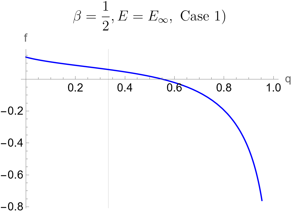
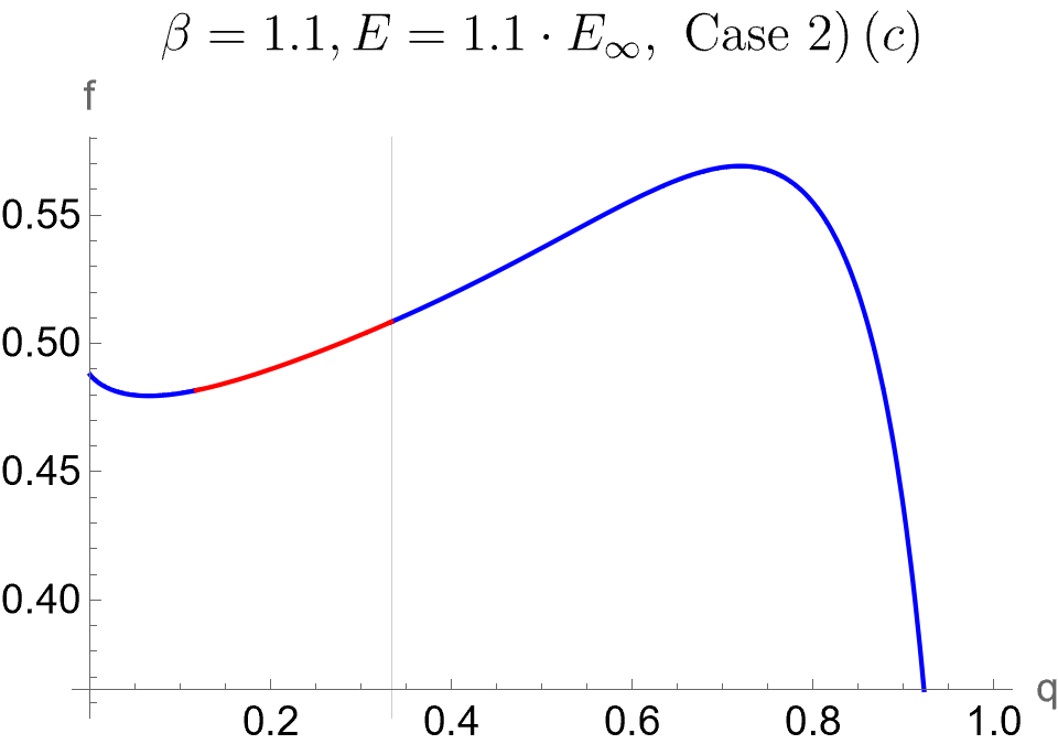
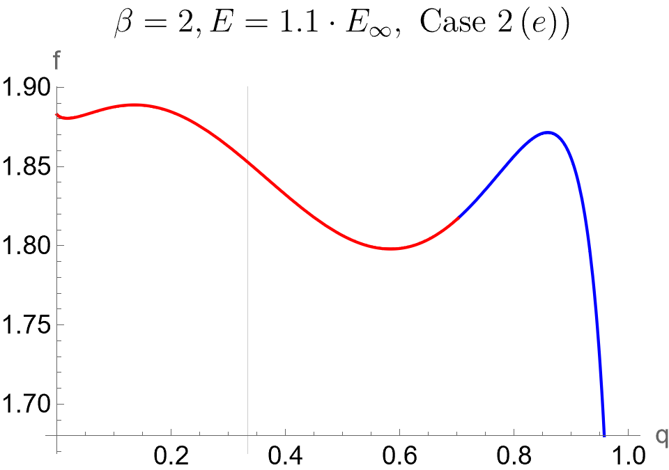
Figure 2. Plots of $f(E,q)$ in $q$ with $p=3$, giving examples for cases 1), 2) (c) and 2) (e). The graph is blue if $q\in D_{\beta}$ and red otherwise. Horizontal line at $q=\frac{p-2}{p}$.

As seen above, for certain values of $E$ and $\beta$ the function $q\to f(E,q)$ may have critical points that are not local maxima or do not satisfy the condition $q\in D_{\beta}$. These physically non-relevant critical points give rise to physically non-relevant TAP solutions.

Proof of Theorem 4.4.

Recall Lemma 4.2. Since the RHS of (4.10) is always at least $1$ it follows that $f$ is decreasing and there are no critical points if $E<E_{\infty}$, proving 1).

Turning to 2), note that the number of critical points is the number of unique solutions to (4.11). If $E=E_{\infty}$ then $r_{-}\left(E/E_{\infty}\right)=r_{+}\left(E/E_{\infty}\right)$ and these are actually one equation, and

$$r_{-}\left(E/E_{\infty}\right)<1<r_{+}\left(E/E_{\infty}\right)\text{ if }E>E_{\infty},$$ (4.20)

so then the equations are distinct. In the latter case it holds thanks to (4.19) that there are no solutions if $\beta/\tilde{\beta}_{c}<r_{-}\left(E/E_{\infty}\right)$, one solution if $\beta/\tilde{\beta}_{c}=r_{-}\left(E/E_{\infty}\right)<r_{+}\left(E/E_{\infty}\right)$, two solutions if $r_{-}\left(E/E_{\infty}\right)<\beta/\tilde{\beta}_{c}<r_{+}\left(E/E_{\infty}\right)$, three solutions if $r_{-}\left(E/E_{\infty}\right)<r_{+}\left(E/E_{\infty}\right)=\beta/\tilde{\beta}_{c}$ and four solutions if $r_{-}\left(E/E_{\infty}\right)<r_{+}\left(E/E_{\infty}\right)<\beta/\tilde{\beta}_{c}$. The fact (4.19) also gives information on if these critical points belong to $(0,\frac{p-2}{p})$ or $(\frac{p-2}{p},1)$, or equal $\frac{p-2}{p}$. Furthermore Lemma 2.1 1) 2) and the fact that $r_{-}\left(E/E_{\infty}\right)<1<r_{+}\left(E/E_{\infty}\right)$ when $E>E_{\infty}$ implies that no critical point arising from $\sqrt{2}\beta_{2}(q)=r_{+}\left(E/E_{\infty}\right)$ is ever in $D_{\beta}$, and all critical points in $(\frac{p-2}{p},1)$ that arise from $\sqrt{2}\beta_{2}(q)=r_{-}\left(E/E_{\infty}\right)$ lie in $D_{\beta}$. In this way all claims about the number and location (but not index) of critical points in 2 a)-e) follow.

The claims about number and location of critical points in 3) similarly follows keeping in mind that if $E=E_{\infty}$ then the two equations in (4.11) coincide.

All claims about number and positions of the critical points in claims 1)-3) are thus proven. To conclude the proof it only remains to determine if the critical points are local maxima, local minima or saddle points. Differentiating (4.12) and using that

$$\xi^{\prime\prime\prime}\left(q\right)\left(1-q\right)-\xi^{\prime\prime}\left(q\right)=p\left(p-1\right)q^{p-3}\left(\left(p-2\right)\left(1-q\right)-q\right)$$

one gets

$$\partial_{q}^{2}f\left(E,q\right)=\beta\frac{p\left(p-2\right)}{4}q^{\frac{p}{2}-2}E-\frac{1}{2\left(1-q\right)^{2}}-\frac{\beta^{2}}{2}p\left(p-1\right)q^{p-3}\left(\left(p-2\right)\left(1-q\right)-q\right).$$ (4.21)

We now show that at a solution to $\partial_{q}f\left(E,q\right)=0$ this factors as

$$\partial_{q}^{2}f\left(E,q\right)=\frac{p}{4q\left(1-q\right)^{2}}\left(q-\frac{p-2}{p}\right)\left(2\beta_{2}\left(q\right)^{2}-1\right).$$ (4.22)

To see this, note that using (4.16) and (1.14) we can make $\beta_{2}\left(q\right)$ appear in the first and last terms of (4.21), and $E_{\infty}$ appear in the first term, obtaining

$$\partial_{q}^{2}f\left(E,q\right)=\frac{p-2}{2q\left(1-q\right)}\sqrt{2}\beta_{2}\left(q\right)\frac{E}{E_{\infty}}-\frac{1}{2\left(1-q\right)^{2}}-\beta_{2}^{2}\left(q\right)\frac{\left(p-2\right)\left(1-q\right)-q}{q\left(1-q\right)^{2}}.$$

Using that at a solution to $\partial_{q}f\left(E,q\right)=0$ the equality (4.10) holds to remove $\frac{E}{E_{\infty}}$ from the expression, we get that at such a point

$$\begin{array}[]{rcl}\partial_{q}^{2}f\left(E,q\right)&=&\displaystyle{\frac{\left(p-2\right)\left(1-q\right)-2q+2\beta_{2}^{2}\left(q\right)\Big{(}\left(p-2\right)\left(1-q\right)-2(\left(p-2\right)\left(1-q\right)-q)\Big{)}}{4q\left(1-q\right)^{2}}}\\ &=&\displaystyle{\frac{\left((p-2)(1-q)-2q\right)\left(2\beta^{2}(q)-1\right)}{4q\left(1-q\right)^{2}}},\end{array}$$ (4.23)

so since $\left(p-2\right)\left(1-q\right)-2q=\left(p-2\right)-pq=-p\left(q-\frac{p-2}{p}\right)$ we obtain that (4.22) holds at any critical point $q$.

By (4.20) solutions of $\sqrt{2}\beta_{2}(q)=r_{-}\left(E/E_{\infty}\right)$ satisfy $2\beta_{2}(q)^{2}<1$ when $E>E_{\infty}$, so that by checking the sign of (4.22) any critical point arising from that equation in $(0,\frac{p-2}{p})$ is a local minimum, and any such critical point in $(\frac{p-2}{p},1)$ is a local maximum. Similarly any solutions of $\sqrt{2}\beta_{2}(q)=r_{+}\left(E/E_{\infty}\right)$ satisfies $2\beta_{2}(q)^{2}>1$ when $E>E_{\infty}$, so that any critical point arising from that equation in $(0,\frac{p-2}{p})$ is a local maximum, and any such critical point in $(\frac{p-2}{p},1)$ is a local minimum. This concludes the identification of all claimed local maxima and minima in 2).

It remains to prove that in the remaining cases the critical points are saddle points. When $E=E_{\infty}$ we have from (4.8)

$$\partial_{q}f(E,q)=-\frac{(\sqrt{2}\beta_{2}(q)-1)^{2}}{2(1-q)}.$$

As this is non-positive and only touches but never crosses $0$ at a finite number of points $f$ is decreasing and all critical points for $E=E_{\infty}$ are saddle points, concluding the proof of claim 3).

Next in the cases 2) (b) (d) recall that all unclassified critical points are at $q=\frac{p-2}{p}$, so that at these points

$$\frac{E}{E_{\infty}}=\frac{1}{2}\left(\frac{1}{\sqrt{2}\beta_{2}\left(\frac{p-2}{p}\right)}+\sqrt{2}\beta_{2}\left(\frac{p-2}{p}\right)\right),$$ (4.24)

giving us from (4.8) and the identity $\frac{1}{x}+x-(\frac{1}{y}+y)=\frac{1}{y}(\frac{1}{x}-y)(y-x)$ that

$$\partial_{q}f(E,q)=\frac{\left(\frac{1}{\sqrt{2}\beta_{2}\left(\frac{p-2}{p}\right)}-\sqrt{2}\beta_{2}(q)\right)\left(\sqrt{2}\beta_{2}(q)-\sqrt{2}\beta_{2}\left(\frac{p-2}{p}\right)\right)}{2(1-q)}.$$

The first factor has the same non-zero sign throughout $(\frac{p-2}{p}-\varepsilon,\frac{p-2}{p})\cup(\frac{p-2}{p},\frac{p-2}{p}+\varepsilon)$ for some small enough $\varepsilon$ (the midpoint $q=\frac{p-2}{p}$ can also be included if $\beta\neq\tilde{\beta}_{c}$; when $\beta=\tilde{\beta}_{c}$ the first factor is zero there) while the second only touches zero (not crossing), since $q=\frac{p-2}{p}$ maximizes $\beta_{2}$. Hence $q=\frac{p-2}{p}$ is a saddle point, concluding the proof of claims 2) (b) (d). This concludes the proof of 1)-3).

∎

We will use the following consequences of the theorem.

Corollary 4.5.

The following holds for all $E$.

1. There is at most one local maximum of $q\to f(E,q)$ in $D_{\beta}$.

2. All local maxima of $q\to f(E,q)$ that lie in $D_{\beta}\setminus\{0\}$ also lie in $(\frac{p-2}{p},1)$.

3. All local maxima in $(\frac{p-2}{p},1)$ satisfy $\sqrt{2}\beta_{2}(q)=r_{-}\left(E/E_{\infty}\right)$.

4. When it exists, the unique local maximum in $D_{\beta}\cap(\frac{p-2}{p},1)$ is the global maximum of $q\to f(E,q)$ in $D_{\beta}\cap(\frac{p-2}{p},1)$.

Proof.

1)-3) follows directly by examining all the possible cases in 1)-3) in the previous theorem. The claim 4) follows since if a differentiable function has only one local maximum and no minima in an interval then this local maximum is the global maximum in the interval. ∎

Lemma 4.1, Theorem 4.4 and Corollary 4.5 strongly constrain which combinations of energy $g(\hat{m})$ at local maximum, norm $|m|^{2}$ of $g$-TAP  solution and $g$-TAP  energy $H_{\operatorname{TAP}}^{g}(m)$ are possible for a relevant $g$-TAP  solution. Let

$$E_{\min}=\begin{cases}\frac{E_{\infty}}{2}\left(\frac{\tilde{\beta}_{c}}{\beta}+\frac{\beta}{\tilde{\beta}_{c}}\right)\geq E_{\infty}&\text{ if }\beta\leq\tilde{\beta}_{c},\\ E_{\infty}&\text{ if }\beta\geq\tilde{\beta}_{c}.\end{cases}.$$ (4.25)

Note that

$$\begin{array}[]{rcl}E>E_{\infty}\text{ and }r_{-}(E/E_{\infty})>\beta/\tilde{\beta}_{c}&\iff&E>E_{\min},\\ E<E_{\infty}\text{ or }\left(E\geq E_{\infty}\text{ and }r_{-}(E/E_{\infty})<\beta/\tilde{\beta}_{c}\right)&\iff&E<E_{\min}\end{array}$$ (4.26)

(recall (4.7)). Thus if $m$ is a relevant TAP solution then by Theorem 4.4 the energy $E=g(\hat{m})$ satisfies $E>E_{\min}$. Also define

$$q_{\min}=\begin{cases}\frac{p-2}{p}&\text{ if }\beta\leq\tilde{\beta}_{c},\\ \text{unique solution of }\sqrt{2}\beta_{2}\left(q\right)=1\text{ in }[\frac{p-2}{p},1)&\text{ if }\beta\geq\tilde{\beta}_{c}.\end{cases}$$ (4.27)

Note that by Lemma 2.1 a) and (4.16)-(4.17) we have

$$D_{\beta}\cap\left[\frac{p-2}{p},1\right]=[q_{\min},1].$$ (4.28)

Later we will use that

$$q_{\min}\text{ is strictly decreasing in }\beta\text{ when }\beta\geq\tilde{\beta}_{c},$$ (4.29)

(recall (4.27), (4.16), (4.17)) and

$$q_{\min}=\frac{p-2}{p-1}\text{ when }\beta=\beta_{d},$$ (4.30)

since when $\beta=\beta_{d}$ and $\hat{q}=\frac{p-2}{p-1}$ we have

$$\sqrt{2}\beta_{2}(\hat{q})\overset{\eqref{eq: beta2 concrete form}}{=}\beta_{d}\sqrt{p(p-1)}\left(1-\hat{q}\right)\hat{q}^{\frac{p-2}{2}}\overset{\eqref{eq: beta d def}}{=}1.$$

Define the function

$$E_{q}:[q_{\min},1)\to[E_{\min},\infty)\text{ by }E_{q}(q)=\frac{E_{\infty}}{2}\left(\frac{1}{\sqrt{2}\beta_{2}(q)}+\sqrt{2}\beta_{2}(q)\right),$$ (4.31)

cf. (4.10). By (4.18) we have $E_{q}(q_{\min})=E_{\min}$ and by (4.17) and since $\sqrt{2}\beta_{2}(q)\leq 1$ for $q\geq q_{\min}$ (see (4.26) and (4.18))

$$E_{q}\text{ is strictly increasing}.$$ (4.32)

Therefore we can define a function

$$q_{E}:[E_{\min},\infty)\to[q_{\min},1)\text{ by }q_{E}=E_{q}^{-1},$$ (4.33)

for which

$$q_{E}\text{ is strictly increasing}.$$ (4.34)

There are several useful ways to characterize $q_{E}$. Since (4.10) and (4.11) are equivalent we have by (4.19) that

$$q_{E}(E)\text{ is the unique solution to }\sqrt{2}\beta_{2}(q)=r_{-}(E/E_{\infty})\text{ in }\left[\frac{p-2}{p},1\right],$$ (4.35)

or equivalently using (4.16) that

$$q_{E}(E)\text{ is the unique solution to }(1-q)q^{\frac{p-2}{p}}=\frac{r_{-}(E/E_{\infty})}{\beta\sqrt{p(p-1)}}\text{ in }\left[\frac{p-2}{p},1\right].$$ (4.36)

Alternatively we have the following.

Lemma 4.6.

For all $\beta\geq 0,E\geq E_{\min}$

$$q_{E}\left(E\right)\text{ is the unique critical point and global maximum of }q\to f\left(E,q\right)\text{ in }D_{\beta}\cap\left[\frac{p-2}{p},1\right],$$ (4.37)

and

$$q_{E}(E)\text{ is a local maximum iff }E>E_{\min}.$$ (4.38)

Proof.

By (4.35), the equivalence of (4.9) and (4.11) and the fact that no solution to $\sqrt{2}\beta_{2}(q)=r_{+}(E/E_{\infty})$ can lie in $D_{\beta}$ it follows that $q_{E}(E)$ is the unique critical point in the interval. By examining all cases in Theorem 4.4 and recalling (4.26) we get (4.38). By Corollary 4.5 4) the claim (4.37) thus follows for $E>E_{\min}$.

The special case $E=E_{\min}$ follows since then $q_{\min}=q_{E}(E_{\min})$ is a critical point of $q\to f(E,q)$ by (4.10), (4.31) and (4.33), which by Theorem 4.4 3) is a saddle point, and is also is the left-endpoint of $D_{\beta}\cap\left[\frac{p-2}{p},1\right]$, and $f(E,q)\to-\infty$ for $q\to 1$, so that the saddle point is the maximum. ∎

We also define

$$U_{\min}=f\left(E_{\min},q_{E}\left(E_{\min}\right)\right),$$ (4.39)

and the function

$$U_{E}\left(E\right)=f\left(E,q_{E}\left(E\right)\right).$$ (4.40)

The fact that $f\left(E,q\right)$ is strictly increasing in $E$ (see (4.3)), $q_{\min}\geq\frac{p-2}{p}$ and (4.37) implies that

$$U_{E}\text{\,is strictly increasing}.$$ (4.41)

Therefore there is a function

$$E_{U}:[U_{\min},\infty)\to[E_{\min},\infty)\text{ defined by }E_{U}=U_{E}^{-1},$$ (4.42)

and

$$E_{U}\text{\,is strictly increasing}.$$ (4.43)

We have the following.

Lemma 4.7.

A vector $m$ is a relevant non-zero $g$-TAP solution of energy $U$ iff $\hat{m}$ is a local maximum of $g$, $U>U_{\min}$, $g(\hat{m})=E_{U}(U)$ and $|m|^{2}=q_{E}(E_{U}(U))$.

Proof.

By Lemma 4.1 1), Theorem 4.4, (4.26) and (4.37)-(4.38) we have that a vector $m$ is a relevant non-zero TAP solution with $g(\hat{m})=E$ iff $\hat{m}$ is a local maximum of $g$, $E>E_{\min}$ and $|m|^{2}=q_{E}(E)$. Since $H^{g}_{\operatorname{TAP}}(m)=U_{E}(g(\hat{m}),|m|^{2})$ we get the claim with the bijective change of variables $U=U_{E}(E)$ and (4.39). ∎

Remark 4.8.

The above lemma implies that (if $g$ is random) there are no relevant g-TAP solutions $m$ of energy $\frac{1}{N}H^{g}_{\rm{TAP}}(m)\leq U_{\min}$ almost surely.

Theorem 4.4 and (4.26) also imply the next lemma.

Lemma 4.9.

If $E>E_{\min}$ then $q\to f(E,q)$ has only one critical point in $D_{\beta}$, which is a local maximum. If $E<E_{\min}$ then $q\to f(E,q)$ has no critical points in $D_{\beta}$.

5. Complexity threshold

In this section we prove Theorem 1.1 about the complexity threshold, using the results of the previous section and the complexity of critical points from (3.8).

Proof of Theorem 1.1.

We first prove (1.20). This implies also implies (1.19) since by Lemma 4.1 2) $m=0$ is a relevant TAP solution almost surely when $\beta\leq\beta_{d}$, so in particular it is when $\beta\leq\beta_{c}<\beta_{d}$.

By Lemma 4.1 1), (4.9)-(4.10) and (4.18) when $\beta\leq\tilde{\beta}_{c}$ any non-zero TAP solution must satisfy

$$H_{N}(\hat{m})\geq\frac{E_{\infty}}{2}\left(\frac{\tilde{\beta}_{c}}{\beta}+\frac{\beta}{\tilde{\beta}_{c}}\right).$$ (5.1)

Note that when $\beta\leq\tilde{\beta}_{c}$

$$\frac{E_{\infty}}{2}\left(\frac{\tilde{\beta}_{c}}{\beta}+\frac{\beta}{\tilde{\beta}_{c}}\right)>E_{0}\iff\frac{1}{2}\left(\frac{\tilde{\beta}_{c}}{\beta}+\frac{\beta}{\tilde{\beta}_{c}}\right)>\frac{E_{0}}{E_{\infty}}\overset{\eqref{eq: rpmdef as sols}}{\iff}\frac{\beta}{\tilde{\beta}_{c}}<r_{-}\left(\frac{E_{0}}{E_{\infty}}\right)\overset{\eqref{eq: rbardef},\eqref{eq: betacdef}}{\iff}\beta<\beta_{c}.$$ (5.2)

Thus the claim (1.19) follows since (1.15) implies that the probability of an $\hat{m}$ satisfying (5.1) existing goes to zero. The claims (1.21) and (1.22) are simple consequences of (1.19) and the definitions (1.8) of $I_{\rm TAP}$ and (1.9) of $f_{\operatorname{TAP}}(\beta)$.

Conversely if $\beta>\beta_{c}$ then we have that

$$r_{-}\left(\frac{E}{E_{\infty}}\right)<\frac{\beta}{\tilde{\beta}_{c}}\text{ for }E\in[E_{0}-\delta,E_{0}],$$

for any $\delta>0$. By Theorem 4.4 2) and (4.37) the function $q\to f(E,q)$ thus has a local maximum $q_{E}$ with $q_{E}\in D_{\beta}\setminus\{0\}$ for all $E\in[E_{0}-\delta,E_{0}]$. This means that if $\hat{m}$ is a critical point of $H_{N}$ with $\frac{1}{N}H_{N}(\hat{m})\in[E_{0}-\delta,E_{0}]$ then $m=q^{p/2}\hat{m}$ is a relevant TAP solution. Thus using the notations from (1.24) and above (1.12)

$$\mathcal{N}_{N}(\mathbb{R},\mathbb{R},D_{\beta}\setminus\{0\})\geq\mathcal{M}([E_{0}-\delta,E_{0})).$$

Taking logs and dividing by $N$ implies (1.23) by the definitions (1.8) and (1.12), since $I([E_{0}-\delta,E_{0}))>0$ for all $\delta>0$ (recall (3.8)). ∎

Remark 5.1.

Eq. (5.2) explains the origin of the threshold $\beta_{c}$: it is the first $\beta$ where critical points of $H_{N}$ of energy as low as $NE_{0}$ give rise to relevant TAP solutions.

6. Computation of the TAP rate function

In this section we give a more detailed version of Theorem 1.2 about the TAP rate function. Define

$$U_{q}(q)=f(E_{q}(q),q)=\beta q^{p/2}E_{q}(q)+\frac{1}{2}\log(1-q)+\operatorname{On}(q).$$ (6.1)

Since $x\to x+1/x$ is strictly decreasing for $x\leq 1$ and $q\to\sqrt{2}\beta_{2}(q)$ is strictly decreasing for $q\geq q_{\min}$ (recall (4.27)) we have that $E_{q}$ is strictly increasing for such $q$. Thus since $U_{q}^{\prime}(q)=\beta q^{p/2}E_{q}^{\prime}(q)+\frac{d}{dq}f(E_{q}(q),q)=\beta q^{p/2}E_{q}^{\prime}(q)>0$ for $q\geq q_{\min}$ we have that

$$U_{q}(q)\text{ is strictly increasing for }q\geq q_{\min}.$$

From (6.1), (4.40) and (4.33) we have the natural relation

$$U_{q}(q)=U_{E}(E_{q}(q)).$$ (6.2)

Recall that from (4.39)

$$U_{\min}=U_{E}(E_{\min})=\begin{cases}U_{E}(E_{\min})&\text{\,if }\beta_{c}\leq\beta\leq\tilde{\beta}_{c},\\ U_{E}(E_{\infty})&\text{\,if }\beta\geq\tilde{\beta}_{c},\end{cases}\text{ and let }U_{\max}=\begin{cases}-\infty&\text{\,if }\beta<\beta_{c},\\ U_{E}(E_{0})&\text{\,if }\beta\geq\beta_{c}.\end{cases}$$ (6.3)

Since $E_{U}=U_{E}^{-1}$ it follows trivially from these that

$$E_{U}(U_{min})=E_{\min}\text{ and }E_{U}(U_{\max})=E_{0}.$$ (6.4)

In Proposition 7.1 we give more concrete formulas for $U_{\min}$ and $U_{\max}$. Our full result on the TAP complexity is the following. There are many ways to express the dependence of the $I_{\operatorname{TAP}}$ on $I$; we choose to present a verbose version and a compact version.

Theorem 6.1 (TAP entropy in terms of critical point entropy).

For all $\beta\geq\beta_{c}$ we have $U_{\min}\leq U_{\max}$, with equality only if $\beta=\tilde{\beta}_{c}$. Furthermore it holds that

$$I_{{\rm TAP}}\left(U,V,q\right)=\begin{cases}I(E_{\min})\overset{\text{for }\beta>\tilde{\beta}_{c}}{>}0&\text{ if }U=U_{\min}\\ &\quad\text{and }q=q_{E}(E_{\min}),V=q^{p/2}E_{\min},\\ I\left(E\right)\in(0,I(E_{\min}))&\text{ if }U_{\min}<U<U_{\max}\\ &\quad\text{and }q\text{\,is the unique solution to }U_{q}\left(q\right)=U\text{ in }[q_{\min},1),\\ &\quad\text{and }V=q^{p/2}E\text{ and }E=E_{q}(q)\in(E_{\min},E_{0})\\ I(E_{0})=0&\text{if }U=U_{\max}\\ &\quad\text{and }q=q_{E}(E_{0}),V=q^{p/2}E_{0},\\ 0&\text{\,if }U=\frac{\beta^{2}}{2}\text{ and }\beta\leq\beta_{d}\\ &\quad\text{and }V=0,q=0,\\ -\infty&\text{otherwise}.\end{cases}$$ (6.5)

Alternatively it holds for all $\beta\geq 0$ and $U$ that

$$I_{\operatorname{TAP}}\left(U,E,q\right)=\begin{cases}I\left(E_{U}\left(U\right)\right)&\text{ if }U\geq U_{\min},q=q_{E}(E_{U}(U)),V=q^{p/2}E_{U}(U),\\ 0&\text{\,if }U=\frac{\beta^{2}}{2},V=0,q=0\text{ and }\beta\leq\beta_{d}\\ -\infty&\text{ otherwise}.\end{cases}$$ (6.6)

Remark 6.2.

a) From (6.6) one sees that for each $U$ there is at most one $(V,q)$ such that $I_{\operatorname{TAP}}(U,V,q)\neq-\infty$.

b) From the first three cases in (6.5) one sees that relevant TAPsolutions of minimal energy $U_{\min}$ are the most numerous, and they have complexity $I(E_{\min})$ ($=I(E_{\infty})$ if $\beta\geq\tilde{\beta}_{c}$, while for any $U>U_{\min}$ the complexity is $I(E)$ for some $E>E_{\min}$ and $I(E)<I(E_{\min})$). Also from the third case one sees that the number of relevant TAP solutions within $o(N)$ of the maximal TAP energy is subexponential, since their complexity $0$.

c) Furthermore combined with (4.25) wee see the meaning of the threshold $\tilde{\beta}_{c}$: for $\beta>\tilde{\beta}_{c}$ all critical points of $H_{N}$ on $S_{N-1}$ of any energy in $[E_{\infty},E_{0}]$ give rise to relevant TAP solutions, while for $\beta\in(\beta_{c},\tilde{\beta}_{c})$ we have $E_{\min}>E_{\infty}$ and only critical points with energies in $[E_{\min},E_{0}]$ do so.

Proof.

Let

$$q_{U}(U)=q_{E}(E_{U}(U))$$ (6.7)

and note that $q_{U}:[U_{\min},\infty)\to[q_{\min},1)$ is strictly increasing (see (4.34) and (4.43)), and $q_{U}=U_{q}^{-1}$ since by definition and (6.2) we have $q_{U}(U_{q}(q))=q_{E}(E_{U}(U_{q}(q))=q$. Also let $V_{U}(U)=q_{U}(U)^{p/2}E_{U}(U)$. Since $q_{U}$ and $E_{U}$ are increasing so is $V_{U}$. Now (6.6) follows essentially directly since by Lemma 4.7 an $m\neq 0$ is a relevant TAP solution of energy $U$ iff $\hat{m}$ is a critical point of $H_{N}$ such that $\frac{1}{N}H_{N}(\hat{m})=E_{U}(U)$, $\frac{1}{N}H_{N}(m)=V_{U}(U)$ and $|m|^{2}=q_{U}(U)$.

The detailed argument is the following. Recall that $E_{U},V_{U},q_{U}$ are strictly increasing. Furthermore they are continuous and differentiable ($E_{q}$ is by (4.31) and (4.16), which implies that the rest are via (4.33), (4.40), (4.42)). Therefore for all $U\in\mathbb{R},\varepsilon>0,\mathcal{V}\subset\mathbb{R},\mathcal{Q}\subset(0,1]$ if $V_{U}\left(U\right)\notin\mathcal{V}$ or $q_{U}\left(U\right)\notin\mathcal{Q}$ then for small enough $\varepsilon$ we have recalling the definitions (1.24) and above (1.12) we have

$$\mathcal{N}_{N}\left(\left[U-\varepsilon,U+\varepsilon\right],\mathcal{V},\mathcal{Q}\right)=-\infty.$$

This implies that

$$I_{{\rm TAP}}\left(U,V,q\right)=-\infty\text{\,if }V\neq V_{U}\left(U\right)\text{\,or }q\notin\{0,q_{U}\left(U\right)\}.$$

Furthermore for any $\varepsilon>0$

$$\begin{array}[]{l}\mathcal{N}_{N}\left(\left[U-\varepsilon,U+\varepsilon\right],\left[V_{U}\left(U-\varepsilon\right),V_{U}\left(U+\varepsilon\right)\right],\left[q_{U}\left(U-\varepsilon\right),q_{U}\left(U+\varepsilon\right)\right]\right)\\ =\mathcal{M}_{N}\left(\left[E_{U}\left(U-\varepsilon\right),E_{U}\left(U+\varepsilon\right)\right]\right)\end{array}$$

This proves that for any $U$, if $V=V_{U}\left(U\right)$ and $q=q_{U}\left(U\right)$ we have

$$I_{{\rm TAP}}\left(U,V,q\right)=I\left(E_{U}\left(U\right)\right).$$

Furthermore for $\varepsilon$ such that $\varepsilon<q_{\min}$ we have

$$\begin{array}[]{l}\mathcal{N}_{N}\left(\mathcal{U},\mathcal{V},[0,\varepsilon)\right)=\begin{cases}1&\text{ if }\frac{\beta^{2}}{2}\in\mathcal{U},0\in\mathcal{V},\beta\leq\frac{\beta^{2}}{2}\\ 0&\text{ otherwise}.\end{cases}\end{array}$$

This implies that

$$I_{{\rm TAP}}\left(U,V,0\right)=\begin{cases}0&\text{ if }\frac{\beta^{2}}{2}\in\mathcal{U},0\in\mathcal{V},\beta\leq\frac{\beta^{2}}{2}\\ -\infty&\text{ otherwise}.\end{cases}$$

Thus the proof of (6.6) is complete.

The first and the third case in (6.5) follows from the fact that $E_{U}(U_{\min})=E_{\min}$, whereby $E_{\min}=E_{\infty}$ if $\beta\geq\tilde{\beta}_{c}$ (recall (4.25)) and $E_{U}(U_{\max})=E_{0}$, which are consequences of the definition (6.3) and the fact that $E_{U}=U_{E}^{-1}$ (recall (4.41)). The second case follows because $E_{U}$ is strictly increasing (recall (4.43)) and (6.4) so that $E_{U}(U)\in(E_{\min},E_{0})$ if $U\in(U_{\min},U_{\max})$, and that $U_{q}(q)=U\iff q=q_{U}(U)\iff q=q_{E}(E_{U}(U))$. ∎

Theorem 1.2 follows from Theorem 6.1, except for the claim that $U_{\max}\leq\beta^{2}/2$. This missing part is in fact a consequence of Theorem 1.5.

Finally we rederive (1.21), this time from Theorem 6.1, in a way that reinforces the point made in Remark 5.1.

Alternative proof (1.21).

We have that

$$\begin{array}[]{c}\beta<\beta_{c}\iff E_{\min}>E_{0},\\ \beta=\beta_{c}\iff E_{\min}=E_{0},\\ \beta>\beta_{c}\iff E_{\min}<E_{0},\end{array}$$ (6.8)

since when $\beta\leq\tilde{\beta}_{c}$ first expression in (5.2) is equivalent to $E_{\min}>E_{0}$ by (4.25) and (1.17)-(1.18) and $E_{\min}$ is non-increasing in $\beta$ (recall (4.25)). Therefore

$$\text{when }\beta<\beta_{c}\text{ we have }E_{U}(U)>E_{0}\mbox{ for all }U\geq U_{\min},$$ (6.9)

so that

$$\sup_{q\in(0,1],V\in{\mathbb{R}}}I_{\operatorname{TAP}}(U,V,q)\overset{\eqref{eq: TAP comp}}{=}I(E_{U}(U))\overset{\eqref{eq: EU at least E0}}{>}I(E_{0})=0,$$

which implies that the RHS in fact equals $-\infty$, giving (1.21). ∎

7. Maximal and minimal TAP energy

In this section we give more concrete formulas for $U_{\min}$ and $U_{\max}$ when $\beta\geq\beta_{c}$.

Proposition 7.1.

It holds for $\beta\geq\tilde{\beta}_{c}$ that

$$U_{\min}=\begin{cases}\frac{\beta^{2}}{2}+\frac{1}{2}\log\frac{2}{p}+\frac{p-2}{8p}\left(4+\frac{\beta^{2}}{\tilde{\beta}_{c}^{2}}\frac{p-2}{p-1}\right)&\text{\,if }\beta_{c}\leq\beta\leq\tilde{\beta}_{c},\\ \frac{\beta^{2}}{2}+\frac{1}{2}\log\left(1-q\right)+\frac{q\left(3p\left(1-q\right)+3q-4\right)}{\left(1-q\right)^{2}2p\left(1-p\right)}&\text{\,if }\beta\geq\tilde{\beta}_{c}\\ \text{where }q\text{\,is the unique solution to }\\ \left(1-q\right)q^{\frac{p-2}{2}}=\frac{1}{\beta\sqrt{p\left(p-1\right)}}\text{ in }[\frac{p-2}{p},1).\end{cases},$$ (7.1)

and

$$\begin{array}[]{lll}U_{\max}&=&\frac{\beta^{2}}{2}+\frac{1}{2}\log\left(1-q\right)+\frac{2}{p}\frac{q}{1-q}\frac{E_{0}}{E_{\infty}}\bar{r}-\frac{1}{2}\frac{p+\frac{q}{1-q}}{p(p-1)}\frac{q}{1-q}\bar{r}^{2}\\ &&\text{ where }q\text{\,is the unique solution to}\\ &&\left(1-q\right)q^{\frac{p-2}{2}}=\frac{\bar{r}}{\sqrt{p\left(p-1\right)}}\text{ in }(\frac{p-2}{p},1),\end{array}$$ (7.2)

or alternatively

$$U_{\max}=\sup_{q\geq\frac{p-2}{p}:\sqrt{2}\beta_{2}(q)\leq 1}h_{\operatorname{TAP}}(q^{p/2}E_{0},q)$$ (7.3)

The following identity will be useful in this section and the next.

Lemma 7.2.

For any $E,q$ we have

$$f\left(E,q\right)=\frac{\beta^{2}}{2}+\frac{1}{2}\log\left(1-q\right)+\frac{E}{E_{\infty}}\frac{2}{p}\frac{q}{1-q}w-\frac{1}{2}\left(p\left(1-q\right)+q\right)\frac{1}{p\left(p-1\right)}\frac{q}{\left(1-q\right)^{2}}w^{2},$$ (7.4)

where $w=\sqrt{2}\beta_{2}(q)$.

Proof.

By (4.16) we have

$$\beta q^{p/2}=\frac{w}{\sqrt{p\left(p-1\right)}}\frac{q}{1-q}\text{ for all }q,\beta.$$ (7.5)

Thus for the first term of $f\left(E,q\right)$ in (4.3) we have that

$$\beta Eq^{p/2}\overset{E_{\infty}=2\sqrt{\frac{p-1}{p}}}{=}\frac{E}{E_{\infty}}\frac{2}{p}\frac{q}{1-q}w$$

for all $q$. By (4.5) the last term of $f\left(E,q\right)$ equals

$$\begin{array}[]{lcl}\frac{\beta^{2}}{2}\left(1-p\left(1-q\right)q^{p-1}-q^{p}\right)&=&\frac{\beta^{2}}{2}-\frac{\beta^{2}}{2}q^{p-1}\left(p\left(1-q\right)+q\right)\\ &\overset{\eqref{eq: beta2 concrete form}}{=}&\frac{\beta^{2}}{2}-\frac{1}{2}\left(\sqrt{2}\beta_{2}\left(q\right)\right)^{2}\frac{1}{p\left(p-1\right)}\frac{q}{\left(1-q\right)^{2}}\left(p\left(1-q\right)+q\right),\end{array}$$

for all $q$. Thus (7.4) follows. ∎

Proof of Proposition 7.1.

Recall from (6.3) and (4.39)-(4.40) that $U_{\min}=f(E_{\min},q_{\min})$ and $U_{\max}=f(E_{0},q_{E}(E_{0}))$. The latter with (4.37) implies (7.3).

From (4.36) we have that $q_{\min}=q_{E}(E_{\min})$ satisfies $w=\sqrt{2}\beta_{2}(q_{\min})=\frac{\beta}{\tilde{\beta}_{c}}$ for $\beta\leq\tilde{\beta}_{c}$ and $w=\sqrt{2}\beta_{2}(q_{\min})=1$ for $\beta\geq\tilde{\beta}_{c}$.

When $\beta\in[\beta_{c},\tilde{\beta}_{c}]$ we have $E_{\min}=\frac{E_{\infty}}{2}\left(\frac{\tilde{\beta}_{c}}{\beta}+\frac{\beta}{\tilde{\beta}_{c}}\right)$ by (4.25). Thus in this case using Lemma 7.2 we get that

$$U_{\min}=\frac{\beta^{2}}{2}+\frac{1}{2}\log\frac{2}{p}+\left(\frac{\beta}{\tilde{\beta}_{c}}+\frac{\tilde{\beta}_{c}}{\beta}\right)\frac{1}{p}\frac{q}{1-q}\frac{\beta}{\tilde{\beta}_{c}}-\frac{1}{2}\left(p\left(1-q\right)+q\right)\frac{1}{p\left(p-1\right)}\frac{q}{\left(1-q\right)^{2}}\frac{\beta^{2}}{\tilde{\beta}_{c}^{2}},$$

where $q=q_{\min}$. Since by (4.27) we have $q_{\min}=\frac{p-2}{p}$ this simplifies to the first line of the LHS of (7.1).

When $\beta\geq\tilde{\beta}_{c}$ we have $E_{\min}=E_{\infty}$. By (4.27) and (4.16) we get that $q=q_{\min}=q_{E}(E_{\infty})$ is the unique solution to the equation in the bottom line of the LHS of (7.1). Thus by Lemma 7.2 we get that

$$U_{\min}=\frac{\beta^{2}}{2}+\frac{1}{2}\log\left(1-q\right)+\frac{2}{p}\frac{q}{1-q}-\frac{1}{2}\left(p\left(1-q\right)+q\right)\frac{1}{p\left(p-1\right)}\frac{q}{\left(1-q\right)^{2}},$$

where $q=q_{\min}$, which simplifies to the second line of (7.1).

Moving to $U_{\max}$, we have that $q_{E}(E_{0})$ solves the equation in (7.2) by (4.36). By Lemma 7.2 we get that

$$U_{\max}=\frac{\beta^{2}}{2}+\frac{1}{2}\log(1-q)+\frac{E_{0}}{E_{\infty}}\frac{2}{p}\frac{q}{1-q}\bar{r}-\frac{1}{2}\left(p\left(1-q\right)+q\right)\frac{1}{p\left(p-1\right)}\frac{q}{\left(1-q\right)^{2}}\bar{r}^{2},$$

which simplifies to the first line on the LHS of (7.2). ∎

8. Solution of the optimization problem

This section is devoted to the analysis of the TAP free energy

$$f_{\operatorname{TAP}}(\beta)=\sup_{U\in\mathbb{R},V\in\mathbb{R},q\in D_{\beta}}\{U+I_{\operatorname{TAP}}(U,V,q)\}$$ (8.1)

and the proofs of Theorems 1.3-1.5. First we rewrite the optimization over $U$ as an optimization over $E$ and $q$ as follows:

Lemma 8.1.

For any $\beta\geq 0$ and $U\geq U_{\min},q\neq 0$

$$U+I_{{\rm TAP}}\left(U,V,q\right)=\begin{cases}f\left(E,q\right)+I\left(E\right)&\text{\,if }q=q_{E}\left(E\right),V=q^{p/2}E\text{\,for }E=E_{U}(U),\\ -\infty&\text{ otherwise}.\end{cases}$$ (8.2)

where $f(E,q)$ is defined in (4.3), $q_{E}$ in (4.37) and $E_{U}$ in (4.42). Also

$$\begin{array}[]{ccc}\displaystyle{\sup_{U\in\mathbb{R},V\in\mathbb{R},q\in D_{\beta}\setminus\{0\}}}\left\{U+I_{\operatorname{TAP}}\left(U,V,q\right)\right\}&=&\displaystyle{\sup_{E\in[E_{\min},E_{0}]}}\left\{f\left(E,q_{E}(E)\right)+I\left(E\right)\right\}\\ &=&\displaystyle{\sup_{E\in[E_{\min},E_{0}],q\in\left[q_{\min},1\right)}}\left\{f\left(E,q\right)+I\left(E\right)\right\}.\end{array}$$ (8.3)

Proof.

For any $U\geq U_{\min}$ we have $U=U_{E}\left(E_{U}\left(U\right)\right)$ since $E_{U}$ is the inverse of $U_{E}$, and (8.2) then follows from the definition (4.40) of $U_{E}$ and (6.6). From (8.2) the first equality of (8.3) follows since the range of $E_{U}$ is $[E_{\min},\infty)$ and $I(E)=-\infty$ for $E>E_{0}$. The second inequality follows from (4.37) and (4.28)), since the range of $q_{E}$ is $[q_{\min},1)$. ∎

Recall

$$I_{\operatorname{Ann}}(E)=g\left(\frac{E}{E_{\infty}}\right),$$ (8.4)

for $g$ from (3.3) denote the annealed rate function of local maxima. In what follows we will will compute

$$\sup_{E\in[E_{\min},\infty)}\left\{f\left(E,q_{E}(E)\right)+I_{\operatorname{Ann}}\left(E\right)\right\}\overset{\eqref{eq: qE glob max}}{=}\sup_{E\in[E_{\min},\infty),q\in[q_{\min},1)}\left\{f\left(E,q\right)+I_{\operatorname{Ann}}\left(E\right)\right\}$$ (8.5)

Using that $I=I_{\operatorname{Ann}}$ on $[E_{\infty},E_{0}]$ and $I=-\infty$ on $(E_{0},\infty)$ we will be able to derive from this the value of (8.3). Since $q_{E}$ maximizes $q\to f(E,q)$ (see (4.37)) the useful identity

$$\frac{d}{dE}\left\{f\left(E,q_{E}\left(E\right)\right)+I_{\operatorname{Ann}}\left(E\right)\right\}=\partial_{E}f\left(E,q_{E}\left(E\right)\right)+I_{\operatorname{Ann}}^{\prime}\left(E\right)\text{ for }E\geq E_{\min}$$ (8.6)

holds.

To compute (8.5) we will consider the critical point equations

$$\begin{array}[]{ccc}\partial_{E}\left(f(E,q)+I_{\operatorname{Ann}}(E)\right)&=&0,\\ \partial_{q}\left(f(E,q)+I_{\operatorname{Ann}}(E)\right)&=&0.\end{array}$$ (8.7)

The second of these equations is nothing but the equation $\partial_{q}f(E,q)=0$ whose solutions are studied in Section 4. Indeed Lemma 4.2 implies that

$$(\tilde{E},\tilde{q})\text{ satisfies }\partial_{q}f\left(E,q\right)=0\text{\,iff }\frac{\tilde{E}}{E_{\infty}}=\frac{1}{2}\left(\sqrt{2}\beta_{2}\left(\tilde{q}\right)+\frac{1}{\sqrt{2}\beta_{2}\left(\tilde{q}\right)}\right).$$ (8.8)

The following identity will be useful to study the first of equation in (8.7).

Lemma 8.2.

If $E=\frac{E_{\infty}}{2}\left(v+\frac{1}{v}\right)$ for $v\in\left(0,1\right)$ then

$$I_{\operatorname{Ann}}^{\prime}\left(E\right)=\frac{v}{\sqrt{p\left(p-1\right)}}-\sqrt{\frac{p-1}{p}}\frac{1}{v}.$$ (8.9)

Proof.

By (8.4) we have $I_{\operatorname{Ann}}^{\prime}\left(E\right)=\frac{1}{E_{\infty}}g^{\prime}\left(\frac{E}{E_{\infty}}\right).$ Note that

$$\Omega^{\prime}(\eta)=2(\eta-\sqrt{\eta^{2}-1}),$$

(either by direct computation from the RHS of (3.2), or since $\Omega^{\prime}(\eta)$ it is the Stieltjes transform of the semi-circle law, as can be seen from taking the derivative of the integral in (3.2)) so that from (3.3) we have

$$g^{\prime}(\eta)=-4\frac{p-1}{p}\eta+2\left(\eta-\sqrt{\eta^{2}-1}\right).$$

Note that

$$\text{if }\eta=\frac{1}{2}\left(v+\frac{1}{v}\right)\text{ for some }v\in\left(0,1\right)\text{\,then }\sqrt{\eta^{2}-1}=\frac{1}{2}\left(\frac{1}{v}-v\right)$$ (8.10)

so that

$$\frac{g^{\prime}(\eta)}{E_{\infty}}=\frac{1}{E_{\infty}}\left(-2\frac{p-1}{p}\left(v+\frac{1}{v}\right)+2v\right)=\frac{1}{E_{\infty}}\left(\frac{2}{p}v-2\frac{p-1}{p}\frac{1}{v}\right)\overset{\eqref{eq: Einf def}}{=}\frac{v}{\sqrt{p\left(p-1\right)}}-\sqrt{\frac{p-1}{p}}\frac{1}{v}.$$

∎

The identity implies the following about solutions to the second equation of (8.7).

Lemma 8.3.

If $\left(E,q\right)$ satisfies $\partial_{q}f\left(E,q\right)=0$ then at $\left(E,q\right)$ we have

$$\partial_{E}\left(f\left(E,q\right)+I_{\operatorname{Ann}}\left(E\right)\right)=\frac{1}{\sqrt{p}}\left(\frac{w}{\sqrt{p-1}}\frac{1}{1-q}-\frac{\sqrt{p-1}}{w}\right),$$ (8.11)

where $w=\sqrt{2}\beta_{2}(q)$.

Proof.

By the definition (4.3) of $f$ we have

$$\partial_{E}\left(f\left(E,q\right)+I_{\operatorname{Ann}}\left(E\right)\right)=\beta q^{p/2}+I_{\operatorname{Ann}}^{\prime}(E)$$

for all $E,q$. Thus by the previous lemma and (8.8), if $(E,q)$ satisfies $\partial_{q}f(E,q)=0$ then

$$\partial_{E}\left(f\left(E,q\right)+I_{\operatorname{Ann}}\left(E\right)\right)=\beta q^{p/2}+\frac{w}{\sqrt{p\left(p-1\right)}}-\sqrt{\frac{p-1}{p}}\frac{1}{w},$$

where $w=\sqrt{2}\beta_{2}(q)$. Rewriting the first term using (7.5) and simplifying (8.11) follows. ∎

We now solve the critical point equations (8.7).

Lemma 8.4.

If $\beta>\beta_{d}$ the critical point equations (8.7) have two solutions $(\tilde{E},\tilde{q})$ whereby $\tilde{q}$ is any of the two solutions of

$$(1-q)q^{p-2}=\frac{1}{p\beta^{2}},$$ (8.12)

or of the equivalent equation

$$2\beta_{2}(q)^{2}=(p-1)(1-q),$$ (8.13)

and

$$\tilde{E}=\frac{E_{\infty}}{2}\left(\frac{1}{\sqrt{2}\beta_{2}(\tilde{q})}+\sqrt{2}\beta_{2}(\tilde{q})\right).$$ (8.14)

Exactly one of the solutions lies in $[E_{\infty},\infty)\times[q_{\min},1)$, and comes from the unique solution to (8.12) in $[\frac{p-2}{p-1},1]$. Both $\tilde{q}$ and $\tilde{E}$ are strictly increasing as functions of $\beta$.

If $\beta<\beta_{d}$ then at any $(\tilde{E},\tilde{q})\in[E_{\infty},\infty)\times[0,1]$ such that (8.14) holds satsifies

$$\frac{d}{dE}\left(f(E,q)+I_{\operatorname{Ann}}(E)\right)|_{(E,q)=(\tilde{E},\tilde{q})}<0,$$ (8.15)

and so the critical point equations (8.7) have no solution in $[E_{\infty},\infty)\times[0,1].$

Remark 8.5.

Recall from (4.30) that $q_{\min}>\frac{p-2}{p-1}$ when $\beta>\beta_{d}$, so then $[q_{\min},1)\subset[\frac{p-2}{p-1},1]$.

Proof.

By (8.8) and the previous lemma a $(\tilde{E},\tilde{q})$ which satisfies (8.14) also satisfies

$$\partial_{E}\left(f\left(E,q\right)+I_{\operatorname{Ann}}\left(E\right)\right)|_{(E,q)=(\tilde{E},\tilde{q})}=\frac{(p-1)(1-\tilde{q})}{w(1-\tilde{q})\sqrt{p(p-1)}}\left(\frac{w^{2}}{(p-1)(1-\tilde{q})}-1\right).$$

Now by (4.16) we have

$$\frac{w^{2}}{(p-1)(1-q)}=p\beta^{2}(1-q)q^{\frac{p-2}{2}},$$

and

$$q\to p\beta^{2}\left(1-q\right)q^{p-2}\text{\,is maximized at }\frac{p-2}{p-1}\text{ where it takes the value }\left(\frac{\beta}{\beta_{d}}\right)^{2},$$ (8.16)

(recall (1.28)) and strictly decreasing thereafter. This implies (8.15). It also implies that indeed (8.12), (8.13) has two solutions if $\beta>\beta_{d}$, one in $(0,\frac{p-2}{p-1})$ and one in $(\frac{p-2}{p-1},1)$, that each of these correspond to a solution of (8.7), and that there are no other solutions of (8.7). Since $p\beta^{2}(1-q)q^{p-2}$ is increasing in $\beta$ this also shows that $\tilde{q}$ is increasing in $\beta$, and since $\sqrt{2}\beta_{2}(q)$ is increasing in $\beta$ (recall (4.16)) we get from (8.14) that $\tilde{E}$ is also increasing in $\beta$. It only remains to show the larger solution to (8.12), (8.13) in fact lies in $[q_{\min},1)$. It can be checked that $\sqrt{p(p-1)}(1-q)q^{\frac{p-2}{2}}\leq p\beta^{2}(1-q)q^{p-2}$ for $q\geq\frac{p-2}{p-1},\beta>\beta_{d}$, and from this (4.16), (4.27) and (8.12) that claim follows. ∎

The following identity will be useful to compute $f(E,q)+I(E)$.

Lemma 8.6.

If $\eta=\frac{1}{2}\left(v+\frac{1}{v}\right)$ for some $v\in\left(0,1\right)$ then

$$I_{\operatorname{Ann}}\left(E_{\infty}\eta\right)=g\left(\eta\right)=\frac{1}{2}\left(v+\frac{1}{v}\right)\left(v-\frac{p-1}{p}\left(v+\frac{1}{v}\right)\right)-\log\frac{v}{\sqrt{p-1}}.$$ (8.17)

Proof.

We have

$$\Omega\left(\eta\right)\overset{\eqref{eq: omega},\eqref{eq: eta v ident}}{=}\frac{1}{2}v^{2}-\log v,$$

so that by (3.3) and (8.10)

$$I_{\text{Ann}}\left(E_{\infty}\eta\right)=g\left(\eta\right)=\frac{1}{2}-\frac{p-1}{p}\frac{1}{2}\left(v+\frac{1}{v}\right)^{2}+\frac{1}{2}v^{2}-\log\frac{v}{\sqrt{p-1}},$$ (8.18)

giving (8.17). ∎

Next we compute the value of $f(E,q)+I(E)$ when $\beta>\beta_{d}$ at the unique solution from Lemma 8.4 with $q\geq q_{\min}$.

Lemma 8.7.

Assume $\beta>\beta_{d}$. The unique solution $(\tilde{E},\tilde{q})$ of (8.7) with $\tilde{q}\geq q_{\min}$ from Lemma 8.4 satisfies

$$f\left(\tilde{E},\tilde{q}\right)+I_{\operatorname{Ann}}\left(\tilde{E}\right)=\frac{\beta^{2}}{2},$$ (8.19)

and

$$I_{\operatorname{Ann}}(\tilde{E})=-\frac{\tilde{q}}{2}-\frac{1}{2p}\frac{\tilde{q}^{2}}{1-\tilde{q}}-\frac{1}{2}\log(1-\tilde{q}).$$ (8.20)

Proof.

We evaluate (7.4) and (8.17) at $(\tilde{E},\tilde{q})$. By (8.13) we have

$$\frac{1}{1-\tilde{q}}=\frac{p-1}{w^{2}}$$ (8.21)

as well as

$$p\left(1-\tilde{q}\right)+\tilde{q}=\left(p-1\right)\left(1-\tilde{q}\right)+1=w^{2}+1.$$ (8.22)

With these identities the last term of (7.4) becomes $\frac{1}{2}\frac{p-1}{p}\left(w+\frac{1}{w}\right)\frac{\tilde{q}}{w}$. Using also $\frac{\tilde{E}}{E_{\infty}}=\frac{1}{2}\left(w+\frac{1}{w}\right)$ the third term of (7.4) becomes $\frac{p-1}{p}\left(w+\frac{1}{w}\right)\frac{\tilde{q}}{w}$, so we get that

$$f\left(\tilde{E},\tilde{q}\right)=\frac{1}{2}\beta^{2}+\frac{1}{2}\log\left(1-\tilde{q}\right)+\frac{1}{2}\frac{p-1}{p}\left(w+\frac{1}{w}\right)\frac{\tilde{q}}{w}.$$

Also setting $v=w$ the last term of (8.17) becomes $-\frac{1}{2}\log(1-\tilde{q})$ and the last factor of the first term becomes $-\frac{wq}{p(1-q)}$. Thus

$$I_{\operatorname{Ann}}\left(\tilde{E}\right)=-\frac{1}{2}\left(w+\frac{1}{w}\right)\frac{w\tilde{q}}{p(1-\tilde{q})}-\frac{1}{2}\log\left(1-\tilde{q}\right).$$ (8.23)

Adding these we get

$$f\left(\tilde{E},\tilde{q}\right)+I_{\operatorname{Ann}}\left(\tilde{E}\right)=\frac{\beta^{2}}{2}+\frac{1}{2}\left(w+\frac{1}{w}\right)\frac{\tilde{q}}{p}\left(\frac{p-1}{w}-\frac{w}{p(1-\tilde{q})}\right),$$

and the last factor of the last term on the RHS is

$$\frac{p-1}{w}-\frac{w}{p(1-\tilde{q})}=\frac{1}{w}\left(p-1-\frac{w^{2}}{p(1-\tilde{q})}\right)\overset{\eqref{eq: q from w}}{=}0,$$

proving (8.19). Also from (8.23) we get

$$I_{\operatorname{Ann}}\left(\tilde{E}\right)=-\frac{1}{2}\left(w^{2}+1\right)\frac{\tilde{q}}{p(1-\tilde{q})}-\frac{1}{2}\log(1-\tilde{q}),$$

which with (8.22) implies (8.20). ∎

Next we confirm that when $\beta>\beta_{d}$ then $(\tilde{E},\tilde{q})$ is in fact the unique point that achieves the supremum in (8.5). Note that

$$E_{\min}=E_{\infty}\text{ when }\beta>\beta_{d},$$ (8.24)

(recall (4.25) and (1.30)).

Lemma 8.8 (Annealed TAP variational formula equals annealed free energy for $\beta>\beta_{d}$).

If $\beta>\beta_{d}$ then

$$\sup_{E\in[E_{\infty},\infty),q\in[q_{\min},1)}\left\{f\left(E,q\right)+I_{\operatorname{Ann}}\left(E\right)\right\}=\frac{\beta^{2}}{2},$$ (8.25)

and the supremum is achieved at a unique point $(\tilde{E},\tilde{q})$. This point is the unique solution from Lemma 8.4 that lies in $(E_{\infty},\infty)\times(q_{\min},1)$.

Proof.

We must check that the supremum is achieved in $(E_{\infty},\infty)\times(q_{\min},1)$. The claims then follows by Lemmas 8.4 and 8.7.

Note that $f(E,q)+I_{\operatorname{Ann}}(E)\to-\infty$ as $q\to 1$ or $E\to\infty$ (since $I_{\operatorname{Ann}}(E)$ goes to $-\infty$ quadratically and $f(E,q)$ to $\infty$ only linearly as $E\to\infty$). This implies that the supremum of (8.25) must be achieved at a point in $[E_{\infty},\infty)\times[q_{\min},1)$, since $f(E,q)+I_{\operatorname{Ann}}(E)$ is continuous on this set.

Considering the border $E=E_{\infty}$ note that using (8.9) with $v=1$ it holds for all $q\geq q_{\min}\geq(p-2)/(p-1)$ (recall (4.30)) that

$$\frac{\partial}{\partial E}\left(f(E,q)+I_{\operatorname{Ann}}(E)\right)|_{E=E_{\infty}}=\beta q^{\frac{p}{2}}-\frac{p-2}{\sqrt{p(p-1)}}>\beta_{d}\left(\frac{p-2}{p-1}\right)^{\frac{p}{2}}-\frac{p-2}{\sqrt{p(p-1)}}\overset{\eqref{eq: beta d def}}{=}0,$$ (8.26)

showing that the supremum of (8.25) is achieved at a point in $(E_{\infty},\infty)\times[q_{\min},1)$. Finally, by Lemma 4.9, for all $E>E_{\infty}$ the function $q\to f(E,q)$ has only one critical point in $(q_{\min},1)$ which is a local maximum, which implies that the supremum is in fact achieved at a point in $(E_{\infty},\infty)\times(q_{\min},1)$. Thus the maximizer must satisfy (8.7), so it is the unique solution $(\tilde{E},\tilde{q})$ from Lemma 8.4. By Lemma 8.7 the equality follows. ∎

Next we turn our attention to the value of the RHS of (8.5) when $\beta<\beta_{d}$.

Lemma 8.9.

For $\beta\in[0,\beta_{d})$ it holds that $f(E,q_{E}(E))+I_{\operatorname{Ann}}(E)$ is decreasing in $E$ on $[E_{\min},\infty)$.

Proof.

For $E\geq E_{\min}$ note that

$$\frac{d}{dE}\left\{f\left(E,q_{E}\left(E\right)\right)+I_{\operatorname{Ann}}\left(E\right)\right\}\overset{\eqref{eq: useful ident}}{=}\partial_{E}f\left(E,q_{E}\left(E\right)\right)+I_{\operatorname{Ann}}^{\prime}\left(E\right)\overset{\eqref{eq: negative}}{<}0.$$

∎

The next lemma shows that for $\beta<\beta_{d}$ (that is, in static and dynamic high temperature) all non-zero relevant TAP solution have a TAP energy lower than the TAP energy of $m=0$.

Lemma 8.10 (Annealed TAP variational formula for $\beta\leq\beta_{d}$).

For $\beta\in[0,\beta_{d}]$

$$f(E_{\min},q_{\min})+I_{\operatorname{Ann}}(E_{\min})\leq\frac{\beta^{2}}{2},$$ (8.27)

with equality only if $\beta=\beta_{d}$.

Proof.

We evaluate the LHS of (8.27) considering the cases $\beta\in[0,\tilde{\beta}_{c}]$ and $\beta\in[\tilde{\beta}_{c},\beta_{d}]$ separately. In the first case $\beta\in[0,\tilde{\beta}_{c}]$ we have $q_{\min}=\frac{p-2}{p}$ and $\frac{E_{\min}}{E_{\infty}}=\frac{1}{2}\left(w+\frac{1}{w}\right)$ where $w=\frac{\beta}{\tilde{\beta}_{c}}\leq 1$ (recall (4.18), (4.25), (4.27)). Plugging these value for $q$ into (7.4) we get

$$f\left(E_{\min},q_{\min}\right)=\frac{1}{2}\beta^{2}+\frac{1}{2}\log\frac{2}{p}+\frac{1}{2}\left(w+\frac{1}{w}\right)w\frac{p-2}{\textbf{}p}-\frac{1}{2}w^{2}\frac{1}{4}\frac{3p-2}{p}\frac{p-2}{p-1}$$

We also have from (8.17)

$$I_{\text{Ann}}\left(E_{\min}\right)=\frac{1}{2}\left(w+\frac{1}{w}\right)\left(w-\frac{p-1}{p}\left(w+\frac{1}{w}\right)\right)-\log\frac{w}{\sqrt{p-1}},$$

so that letting $x=\frac{2\left(p-1\right)}{pw^{2}}$ we get

$$\begin{array}[]{l}f\left(E_{\min},q_{\min}\right)+I_{\text{Ann}}\left(E_{\min}\right)\\ =\frac{\beta^{2}}{2}+\frac{1}{2}\left(w+\frac{1}{w}\right)w\frac{p-2}{p}+\frac{1}{2}\log x-\frac{1}{2}\frac{3p-2}{p}\frac{1}{4}w^{2}\frac{p-2}{p-1}+\frac{1}{2}\left(w+\frac{1}{w}\right)\left(w-\frac{p-1}{p}\left(w+\frac{1}{w}\right)\right)\\ =\frac{\beta^{2}}{2}+\frac{1}{2}\frac{p-1}{p}\left(w+\frac{1}{w}\right)\left(w-\frac{1}{w}\right)+\frac{1}{2}\log x-\frac{1}{2}\frac{3p-2}{p}\frac{1}{4}w^{2}\frac{p-2}{p-1}\\ =\frac{\beta^{2}}{2}+\frac{1}{2}\left(\frac{p-1}{p}-\frac{3p-2}{p}\frac{1}{4}\frac{p-2}{p-1}\right)w^{2}-\frac{x}{4}+\frac{1}{2}\log x\\ =\frac{\beta^{2}}{2}+\frac{1}{4x}-\frac{x}{4}+\frac{1}{2}\log x.\end{array}$$

Note that $\frac{1}{4z}-\frac{z}{4}+\frac{1}{2}\log z<0$ for all $z>1$. Furthermore since $w\leq 1$ we have $x\geq 2\frac{p-1}{p}>1$. This proves (8.27) in this case.

Next we consider the case $\beta\in[\tilde{\beta}_{c},\beta_{d}]$. In this case $E_{\min}=E_{\infty}$ (recall (4.18) and (4.25)), and from (8.17)

$$I_{\text{Ann}}\left(E_{\infty}\right)=-\frac{p-2}{p}+\frac{1}{2}\log\left(p-1\right).$$ (8.28)

Also from (7.4), recalling that $\sqrt{2}\beta(q_{\min})=1$ by (4.27), we get that with $r=\frac{q_{\min}}{1-q_{\min}}$ or equivalently $1-q_{\min}=\frac{1}{1+r}$ that

$$f\left(E_{\min},q_{\min}\right)=\frac{\beta^{2}}{2}-\frac{1}{2}\log\left(1+r\right)+\frac{2}{p}r-\frac{1}{2}r\frac{1}{p-1}-\frac{1}{2}r^{2}\frac{1}{p\left(p-1\right)}.$$

Now (4.30) implies that $q_{\min}\geq\frac{p-2}{p-1}$ for $\beta\leq\beta_{d}$ with equality only if $\beta=\beta_{d}$. Since $q_{\min}\geq\frac{p-2}{p-1}$ corresponds to $r\geq p-2$ with equality only if $r=p-2$ the claim of the lemma in the case $\beta\in[\tilde{\beta}_{c},\beta_{d}]$ follows once we have shown the bound

$$-\frac{1}{2}\log\left(1+r\right)+\frac{2}{p}r-\frac{1}{2}r\frac{1}{p-1}-\frac{1}{2}r^{2}\frac{1}{p\left(p-1\right)}-\frac{p-2}{p}+\frac{1}{2}\log(p-1)\leq 0\text{ for }r\geq p-2,$$

(cf. (8.28)) with equality only if $r=p-2$. It is easy to verify that the LHS is zero when $r=p-2$. Also the derivative of the LHS is zero when $r=p-2$, and the second derivative is negative for $r\geq p-2$. This gives the bound and finishes the proof of the lemma. ∎

We proceed to derive Theorems 1.3, 1.4 and 1.5. We do so by reconstructing the maximizer of $f(E,q)+I(E)$ from the maximizer of $f(E,q)+I_{\operatorname{Ann}}(E)$ by considering when the maximizer of the latter hits $E=E_{0}$.

Proof of Theorem 1.3.

If $\beta<\beta_{d}$ then by (1.9) and (6.6)

$$f_{\operatorname{TAP}}(\beta)=\max\left(\frac{\beta^{2}}{2},\sup_{U\in\mathbb{R},V\in\mathbb{R},q\in D_{\beta}\setminus\{0\}}\{U+I_{\operatorname{TAP}}(U,V,q)\}\right),$$ (8.29)

where the contribution $\frac{\beta^{2}}{2}$ is due to $q=0,V=0$ (i.e. $m=0$). By Lemmas 8.1, 8.9 and 8.10 we see that the other quantity in the max is strictly smaller. Furthermore the other quantity is an upper bound for $U_{\max}$, proving (1.33). This also shows that (1.31) is well-defined shows all the claims in (1.32), by the second case in (6.6).∎

To prove Theorem 1.4 we need the following characterization of $\beta_{s}$.

Lemma 8.11.

When $\beta>\beta_{d}$ the energy $\tilde{E}$ from Lemma 8.4 satisfies

$$\begin{array}[]{c}\beta<\beta_{s}\iff\tilde{E}<E_{0},\\ \beta=\beta_{s}\iff\tilde{E}=E_{0},\\ \beta>\beta_{s}\iff\tilde{E}>E_{0}\end{array}$$ (8.30)

Proof.

Letting $w=\sqrt{2}\beta_{2}(\tilde{q})$ note that

$$\begin{array}[]{ll}\tilde{E}<E_{0}\overset{\eqref{eq: Etildedef}}{\iff}\frac{1}{2}\left(\frac{1}{w}+w\right)<\frac{E_{0}}{E_{\infty}}\overset{\eqref{eq: rpmdef},\eqref{eq: rpmdef as sols}}{\iff}w>r_{-}\left(\frac{E_{0}}{E_{\infty}}\right)\\ \overset{\eqref{eq: rbardef},\eqref{eq: qtildedef equiv}}{\iff}\sqrt{1-\tilde{q}}\sqrt{p-1}>\bar{r}\iff\tilde{q}<1-\frac{1}{p-1}\bar{r}^{2}.\end{array}.$$

Now recalling that $\tilde{q}$ is increasing in $\beta$ by Lemma 8.4 the claim follows by noting that at $\beta=\beta_{s}$ we have $\tilde{q}=\hat{q}=1-\frac{1}{p-1}\bar{r}^{2}$, which can be verified by observing that

$$p\beta_{s}^{2}(1-\hat{q})\hat{q}^{p-2}\overset{\eqref{betasdef}}{=}1.$$

∎

Proof of Theorem 1.4.

Let $\beta\in(\beta_{d},\beta_{s})$. Then by Lemma 2.1 1) we have $0\not\in D_{\beta}$ so that from (1.9), (8.3) and (8.24)

$$f_{\operatorname{TAP}}(\beta)=\sup_{E\in[E_{\infty},E_{0}],q\in[q_{min},1)}\left\{f(E,q)+I(E)\right\}.$$ (8.31)

By Lemma 8.8 the supremum is $f(\tilde{E},\tilde{q})=\beta^{2}/2$, attained uniquely at $(\tilde{E},\tilde{q})$ with $\tilde{E}>E_{\infty}$, as long as the maximizer $\tilde{E}$ from Lemma 8.8 satisfies $\tilde{E}\in(E_{\infty},E_{0}]$, since then the global maximizer is within the region where $I_{\operatorname{Ann}}=I$. This with the previous lemma proves (1.40). By (1.36) we get that $\tilde{q}$ is the unique solution to (1.36). Since the supremum in (8.31) is uniquely attained, we get from (8.2) and the fact that $E_{U}$ is a bijection from $[U_{\min},\infty)$ to $[E_{\min},\infty)$ that the supremum in (1.31) is uniquely attained, so that $U_{*},V_{*},q_{*}$ are well-defined and $U_{*}=f(\tilde{E},q_{*}),V_{*}=q_{*}^{p/2}\tilde{E},q_{*}=\tilde{q}$, which implies (1.37) and (1.38) (recall (8.14)). That $\tilde{E}\in(E_{\infty},E_{0})$ together with (6.3) implies (1.41). Lastly the identity (1.39) follows from (8.20) and the inequality since $\tilde{E}\in(E_{\infty},E_{0})$ and (3.8). ∎

Proof of Theorem 1.5.

Let $\beta>\beta_{s}$. By Lemma 2.1 1) we have $0\not\in D_{\beta}$ so that from (1.9) and (8.3)

$$f_{\operatorname{TAP}}(\beta)=\sup_{E\in[E_{\infty},E_{0}]}\left\{f(E,q_{E}(E))+I(E)\right\}$$ (8.32)

Note that

$$E\to f(E,q_{E}(E))+I(E)$$ (8.33)

has exactly one critical point $E\geq E_{\infty}$ by (8.4), (8.6) and (4.37). Also

$$\frac{d}{dE}\left(f(E,q_{E}(E))+I(E)\right)|_{E=E_{\infty}}\overset{\eqref{eq: qE glob max}}{=}{\partial_{E}}f(E_{\infty},q_{\min})+I^{\prime}(E_{\infty})\overset{\eqref{eq: deriv at Einf}}{>}0.$$

This shows that the unique maximizer $(\tilde{E},\tilde{q})$ of $f(E,q_{E}(E))+I_{\operatorname{Ann}}(E)$ from Lemma 8.10 satisfies $\tilde{E}>E_{0}$ when $\beta>\beta_{s}$ (recall (8.30)) the maximizer of (8.33) in $[E_{\infty},E_{0}]$ must be $E=E_{0}$, and

$$f_{\operatorname{TAP}}(\beta)=f(E_{0},q_{E}(E_{0}))+I(E_{0})=f(E_{0},q_{E}(E_{0}))<f(\tilde{E},q_{E}(\tilde{E}))=\frac{\beta^{2}}{2}.$$

This proves (1.45). By (4.36) we have that $q_{*}=q_{E}(E_{0})$ is the unique solution to (1.42). By (8.2) and the fact the supremum in (8.32) is uniquely attained, so that (1.31) is well-defined and (1.43) (a), (b) and (1.45) follow. Since $f(E_{0},q_{E}(E_{0}))=h_{\operatorname{TAP}}(q^{p/2}E_{0},q)$ and using (7.3)-(7.2) we also obtain (1.44). ∎

References

• [AAČ13] Antonio Auffinger, Gérard Ben Arous and Jiří Černý “Random Matrices and Complexity of Spin Glasses” In Communications on Pure and Applied Mathematics 66.2, 2013, pp. 165–201 DOI: 10.1002/cpa.21422
• [AJ19] Antonio Auffinger and Aukosh Jagannath “On Spin Distributions for Generic p-Spin Models” In Journal of Statistical Physics 174.2, 2019, pp. 316–332 DOI: 10.1007/s10955-018-2188-5
• [AJ19a] Antonio Auffinger and Aukosh Jagannath “Thouless–Anderson–Palmer equations for generic $p$-spin glasses” In The Annals of Probability 47.4, 2019 DOI: 10.1214/18-AOP1307
• [AJ21] Gérard Ben Arous and Aukosh Jagannath “Shattering Versus Metastability in Spin Glasses” arXiv: 2104.08299 In arXiv:2104.08299 [math-ph], 2021 URL: http://arxiv.org/abs/2104.08299
• [BBM96] A Barrat, R Burioni and M Mézard “Dynamics within metastable states in a mean-field spin glass” In Journal of Physics A: Mathematical and General 29.5, 1996, pp. L81–L87 DOI: 10.1088/0305-4470/29/5/001
• [Bel22] David Belius “High temperature TAP upper bound for the free energy of mean field spin glasses” arXiv, 2022 DOI: 10.48550/ARXIV.2204.00681
• [BK19] David Belius and Nicola Kistler “The TAP–Plefka Variational Principle for the Spherical SK Model” In Communications in Mathematical Physics 367.3 Springer, 2019, pp. 991–1017
• [BM80] Alan J Bray and Michael A Moore “Metastable states in spin glasses” Publisher: IOP Publishing In Journal of Physics C: Solid State Physics 13.19, 1980, pp. L469
• [Bol14] Erwin Bolthausen “An Iterative Construction of Solutions of the TAP Equations for the Sherrington–Kirkpatrick Model” In Communications in Mathematical Physics 325.1, 2014, pp. 333–366 DOI: 10.1007/s00220-013-1862-3
• [BSZ20] Gérard Ben Arous, Eliran Subag and Ofer Zeitouni “Geometry and Temperature Chaos in Mixed Spherical Spin Glasses at Low Temperature: The Perturbative Regime” In Communications on Pure and Applied Mathematics 73.8, 2020, pp. 1732–1828 DOI: 10.1002/cpa.21875
• [BY21] Christian Brennecke and Horng-Tzer Yau “A Note on the Replica Symmetric Formula for the SK Model” arXiv: 2109.07354 In arXiv:2109.07354 [math-ph], 2021 URL: http://arxiv.org/abs/2109.07354
• [Cav+03] Andrea Cavagna, Irene Giardina, Giorgio Parisi and Marc Mézard “On the formal equivalence of the TAP and thermodynamic methods in the SK model” Publisher: IOP Publishing In Journal of Physics A: Mathematical and General 36.5, 2003, pp. 1175
• [Cha10] Sourav Chatterjee “Spin glasses and Stein’s method” In Probability Theory and Related Fields 148.3-4, 2010, pp. 567–600 DOI: 10.1007/s00440-009-0240-8
• [CHS93] A. Crisanti, H. Horner and H.-J. Sommers “The Sphericalp-Spin Interaction Spin-Glass Model: The Dynamics” In Zeitschrift für Physik B Condensed Matter 92.2, 1993, pp. 257–271 DOI: 10.1007/BF01312184
• [CK93] L.. Cugliandolo and J. Kurchan “Analytical solution of the off-equilibrium dynamics of a long-range spin-glass model” In Physical Review Letters 71.1, 1993, pp. 173–176 DOI: 10.1103/PhysRevLett.71.173
• [CL06] A. Crisanti and L. Leuzzi “Spherical 2 + p Spin-Glass Model: An Analytically Solvable Model with a Glass-to-Glass Transition” In Physical Review B 73.1, 2006, pp. 014412 DOI: 10.1103/PhysRevB.73.014412
• [CP18] Wei-Kuo Chen and Dmitry Panchenko “On the TAP Free Energy in the Mixed p-Spin Models” In Communications in Mathematical Physics 362.1, 2018, pp. 219–252 DOI: 10.1007/s00220-018-3143-7
• [CPS21] Wei-Kuo Chen, Dmitry Panchenko and Eliran Subag “The Generalized TAP Free Energy II” In Communications in Mathematical Physics 381.1, 2021, pp. 257–291 DOI: 10.1007/s00220-020-03887-x
• [CPS22] Wei-Kuo Chen, Dmitry Panchenko and Eliran Subag “Generalized TAP Free Energy” In Communications on Pure and Applied Mathematics, 2022, pp. cpa.22040 DOI: 10.1002/cpa.22040
• [CS92] A. Crisanti and H.-J. Sommers “The Sphericalp-Spin Interaction Spin Glass Model: The Statics” In Zeitschrift für Physik B Condensed Matter 87.3, 1992, pp. 341–354 DOI: 10.1007/BF01309287
• [CS95] A. Crisanti and H.-J. Sommers “Thouless-Anderson-Palmer Approach to the Spherical p-Spin Spin Glass Model” In Journal de Physique I 5.7, 1995, pp. 805–813 DOI: 10.1051/jp1:1995164
• [DY83] Cyrano De Dominicis and A Peter Young “Weighted averages and order parameters for the infinite range Ising spin glass” Publisher: IOP Publishing In Journal of Physics A: Mathematical and General 16.9, 1983, pp. 2063
• [GM84] D.J. Gross and M. Mezard “The simplest spin glass” In Nuclear Physics B 240.4, 1984, pp. 431–452 DOI: 10.1016/0550-3213(84)90237-2
• [KPV93] J. Kurchan, G. Parisi and M.. Virasoro “Barriers and metastable states as saddle points in the replica approach” In Journal de Physique I 3.8, 1993, pp. 1819–1838 DOI: 10.1051/jp1:1993217
• [MPV87] Marc Mézard, Giorgio Parisi and Miguel Virasoro “Spin glass theory and beyond: An introduction to the replica method and its applications” World Scientific Publishing Company, 1987
• [Sub+17] Eliran Subag “The Complexity of Spherical p -Spin Models—A Second Moment Approach” In The Annals of Probability 45.5 Institute of Mathematical Statistics, 2017, pp. 3385–3450
• [Sub17] Eliran Subag “The geometry of the Gibbs measure of pure spherical spin glasses” In Inventiones mathematicae 210.1, 2017, pp. 135–209 DOI: 10.1007/s00222-017-0726-4
• [Sub20] Eliran Subag “Free energy landscapes in spherical spin glasses” arXiv: 1804.10576 In arXiv:1804.10576 [math], 2020 URL: http://arxiv.org/abs/1804.10576
• [Sub21] Eliran Subag “The free energy of spherical pure <pre>$p$</pre>-spin models – computation from the TAP approach” arXiv: 2101.04352 In arXiv:2101.04352 [cond-mat], 2021 URL: http://arxiv.org/abs/2101.04352
• [Tal10] Michel Talagrand “Mean field models for spin glasses: Volume I: Basic examples” Springer Science & Business Media, 2010
• [TAP77] D.. Thouless, P.. Anderson and R.. Palmer “Solution of ’Solvable Model of a Spin Glass”’ In Philosophical Magazine 35.3, 1977, pp. 593–601 DOI: 10.1080/14786437708235992
• [ZSA21] Zhou Fan, Song Mei and Andrea Montanari “TAP free energy, spin glasses and variational inference” In The Annals of Probability 49.1, 2021, pp. 1–45 DOI: 10.1214/20-AOP1443