Improved Conformalized Quantile Regression

Abstract

Conformalized quantile regression is a procedure that inherits the advantages of conformal prediction and quantile regression. That is, we use quantile regression to estimate the true conditional quantile and then apply a conformal step on a calibration set to ensure marginal coverage. In this way, we get adaptive prediction intervals that account for heteroscedasticity. However, the aforementioned conformal step lacks adaptiveness as described in (Romano et al., 2019). To overcome this limitation, instead of applying a single conformal step after estimating conditional quantiles with quantile regression, we propose to cluster the explanatory variables weighted by their permutation importance with an optimized K-means and apply k conformal steps. To show that this improved version outperforms the classic version of conformalized quantile regression and is more adaptive to heteroscedasticity, we extensively compare the prediction intervals of both in open datasets.

Keywords Conformal prediction  $\cdot$ Conformalized quantile regression  $\cdot$ Conditional coverage  $\cdot$ Group-balanced conformal prediction  $\cdot$ Permutation importance

1 Introduction

Conformal prediction (CP) is a set of distribution-free and model agnostic algorithms devised to predict with a user-defined confidence with coverage guarantee, see Theorem (1.2). CP is key in high risk decision-making settings where the true output must be within the prediction interval (PI) with high probability. Unlike bayesian models [1, 2, 3] that only ensure asymptotic coverage guarantees and bootstrap uncertainty estimations methods [4, 5], CP provides valid coverage in finite samples that work for any model, any distribution, any level $\alpha\in(0,1)$ and any non-conformity score function s, under the mild assumption of exchangeability (see Definition (1)). However, despite being true regardless of the non-conformity score function s, it has a direct impact in prediction intervals (PIs) width and adaptiveness to heteroscedasticity. Therefore, we must clerverly choose the non-conformity score function s to have short as possible adaptive PIs. PIs are said to be adaptive when they take in consideration the uncertainty of the conditional distribution $Y|X$. In plain words, this means that PIs must vary on the input and be wide whenever the model is highly uncertain or the input is indeed hard to predict and narrow if the model has minimal uncertainty on the given input. Unfortunately, conditional coverage, see Eq.(3), is a stronger property that CP does not ensure; however, there are heuristic ways to approximate it.

CP has two main forms: (i) inductive conformal prediction (ICP) and (ii) full conformal prediction [6]. In a nutshell, the former requires data splitting and therefore is more scalable, whereas the latter does not require data splitting at the cost of refitting the model multiple times, thus being computationally onerous. Henceforth, in the interest of scalability, we will solely dedicate to ICP, also referred to as split conformal prediction.

Throughout this paper, we use the notation depicted in Table (1).

Notation	Meaning
$\alpha$	Miscoverage rate $\alpha$
$\hat{C}_{1-\alpha}(\bm{x_{n}})$	$1-\alpha$ prediction interval on input $\bm{x_{n}}$
$x_{(k)}$	k-th rank statistic of $(x_{1},...,x_{n})$
$\bm{\epsilon}$	set of non-conformity scores
Quantile($\bm{\epsilon}$; $1-\alpha$)	$1-\alpha$ order quantile of $\bm{\epsilon}$
$x$	a scalar
$\bm{x}$	a vector
$X$	a matrix or a random variable (easily distinguished)
$\bm{X}$	a tensor or a random vector (easily distinguished)
$(\bm{x_{train}},\bm{x_{cal}},\bm{x_{val}})$	train, calibration and test data, respectively

Table 1: Notation used throughout this paper.

Paper outline

The remainder of this Section does a brief recap on ICP and quantile regression (QR) since the contribution is grounded on it. Section 2 summarizes conformalized quantile regression (CQR) as described in (Romano et al., 2019) [7]. Section 3 introduces our improved version of CQR for tabular data named improved conformalized quantile regression (ICQR). Section 4 extensively compare PIs width and coverage of CQR and ICQR on open datasets and discusses the results. Finally, Section 5 draws the main points and findings of this research, and addresses shortcomings.

1.1 Inductive conformal prediction

The general outline of ICP is as follows:

1. Train a model $\hat{f}$ on a training dataset or use a pre-trained off-the-shelf model;

2. Define a symmetric heuristic notion of uncertainty denoted as $s:\mathcal{X}\times\mathcal{Y}\rightarrow\mathcal{A}\subseteq\mathbb{R}$ usually referred to as the non-conformity score function, where larger scores encode worse agreement between pairs $(\bm{x},y)\in\mathcal{X}\times\mathcal{Y}$;

3. Compute $\epsilon_{1},...,\epsilon_{n}=s(\bm{x_{1}},y_{1}),...,s(\bm{x_{n}},y_{n})$ non-conformity scores on a calibration dataset, not seen by the model during training, using the trained model $\hat{f}$, and the non-conformity score function s applied on pairs of a calibration dataset $\mathcal{D}_{cal}:=\{(\bm{x_{i}},y_{i})\}_{i=1}^{n}$;

4. Compute $\hat{q}=\text{Quantile}\left(\bm{\epsilon};\frac{\lceil(n+1)(1-\alpha)\rceil}{n}\right)$;

5. Deploy PIs as $\hat{C}_{1-\alpha}(\bm{x_{n+1}})=\{y\in\mathcal{Y}:s(\bm{x_{n+1}},y)\leq\hat{q}\}$.

Definition 1 (Exchangeability).

A sequence of random variables $Z_{1},Z_{2},...,Z_{n}\in\mathcal{Z}$ are exchangeable if and only if for any permutation $\pi:\{1,2,...,n\}\rightarrow\{1,2,...,n\}$ and every measurable set $E\subseteq\mathcal{Z}^{n}$, we have

$$\mathbb{P}\{(Z_{1},Z_{2},...,Z_{n})\in E\}=\mathbb{P}\{(Z_{\pi(1)},Z_{\pi(2)},...,Z_{\pi(n)})\in E\}$$ (1)

Lemma 1.1.

Let $Z_{1},...,Z_{n}\in\mathcal{Z}$ be exchangeable random variables with no ties almost surely, then their ranks are uniformly distributed on {1,…,n}.

Proof.

Let $R_{i}=\text{Rank}(Z_{i})$. Since $(Z_{1},...,Z_{n})$ are exchangeable, we have a total of n! possible permutations between them all being equally probable. Additionally, given that $Z_{1},...,Z_{n}$ have no ties almost surely, then $\mathbb{P}(R_{i}\neq R_{j})=1,\quad\forall i\neq j\in\{1,...,n\}$. For any $i\in\{1,...,n\}$, if we fix $R_{i}$ on rank $j\in\{1,...,n\}$, there are (n-1)! possible permutations among the other n-1 random variables. Hence, $\mathbb{P}(R_{i}=j)=\frac{(n-1)!}{n!}=\frac{1}{n}$ and thus

$$\mathbb{P}(R_{i}=1)=\mathbb{P}(R_{i}=2)=...=\mathbb{P}(R_{i}=n)=\frac{1}{n},\quad\forall i\in\{1,...,n\}.$$

∎

Theorem 1.2 (Marginal coverage guarantee).

Let $(\bm{X_{1}},Y_{1}),...,(\bm{X_{n}},Y_{n})$ be exchangeable random vectors with no ties almost surely drawn from a distribution P, additionally if for a new pair $(\bm{X_{n+1}},Y_{n+1})$, $(\bm{X_{1}},Y_{1}),...,(\bm{X_{n+1}},Y_{n+1})$ are still exchangeable, then by constructing $C_{1-\alpha}(\bm{X_{n+1}})$ using ICP, the following inequality holds for any non-conformity score function $s:\mathcal{X}\times\mathcal{Y}\rightarrow\mathcal{A}\subseteq\mathbb{R}$ and any $\alpha\in(\frac{1}{n+1},1)$

$$1-\alpha\leq\mathbb{P}\{Y_{n+1}\in C_{1-\alpha}(\bm{X_{n+1}})\}\leq 1-\alpha+\frac{1}{n+1}.$$ (2)

Proof.

Since $\bm{Z_{1}}=(\bm{X_{1}},Y_{1}),...,\bm{Z_{n}}=(\bm{X_{n}},Y_{n})$ are exchangeable random vectors with no ties almost surely, the corresponding non-conformity scores $\bm{\epsilon}=\{(\epsilon_{i}:=s(\bm{Z_{i}}))\}_{i=1}^{n}\subseteq\mathcal{A}$ are also exchangeable (see Theorem 3 of [8]) with no ties almost surely. Since the non-conformity scores $\epsilon_{1},...,\epsilon_{n},\epsilon_{n+1}$ are exchangeable, their ranks are uniformly distributed by Lemma (1.1). Therefore, $\text{Rank}(\epsilon_{n+1})\sim\mathcal{U}\{1,n+1\}$. That is,

$$\mathbb{P}\{\epsilon_{n+1}\leq\epsilon_{(k)}\}=\mathbb{P}\{\text{Rank}(\epsilon_{n+1})\leq k\}=\frac{k}{n+1},\quad k\in\{1,...,n+1\}.$$

By definition, since $\hat{q}=\text{Quantile}(\bm{\epsilon};\frac{\lceil(n+1)(1-\alpha)\rceil}{n})=\epsilon_{(\lceil(n+1)(1-\alpha)\rceil)}$, follows that

$$\mathbb{P}\{Y_{n+1}\in C_{1-\alpha}(\bm{X_{n+1})}\}=\mathbb{P}\{y\in\mathcal{Y}:s(\bm{X_{n+1}},y)\leq\hat{q}\}=\mathbb{P}\{\epsilon_{n+1}\leq\epsilon_{(\lceil(n+1)(1-\alpha)\rceil)}\}=\frac{\lceil(n+1)(1-\alpha)\rceil}{n+1}.$$

It is easy to note that $1-\alpha\leq\frac{\lceil(n+1)(1-\alpha)\rceil}{n+1}\leq\frac{(n+1)(1-\alpha)+1}{n+1}=1-\alpha+\frac{1}{n+1}$. ∎

As a consequence of Theorem (1.2), ICP provides asymptotic exact coverage since $\lim_{n\rightarrow+\infty}(1-\alpha+\frac{1}{n+1})=1-\alpha\implies\mathbb{P}\{Y_{n+1}\in C_{1-\alpha}(\bm{X_{n+1}})\}=1-\alpha$. In practice, $\text{Quantile}(\bm{\epsilon};\frac{\lceil(n+1)(1-\alpha)\rceil}{n})$, is essentially a very minor finite sample correction on the $1-\alpha$ quantile. However, henceforth, for simplicity, we will use $\text{Quantile}(\bm{\epsilon};1-\alpha)$, but bear in mind that $\text{Quantile}(\bm{\epsilon};\frac{\lceil(n+1)(1-\alpha)\rceil}{n})$ is the formally correct form.

Definition 2 (Conditional coverage).

An ICP procedure guarantees conditional coverage if

$$\mathbb{P}(Y_{val}\in C_{1-\alpha}(\bm{X_{val}})|\bm{X}=\bm{x_{val}})\geq 1-\alpha.$$ (3)

1.2 Naive method

The most basic and widely used non-conformity score function for regression problems is the absolute error given by

$$s(\bm{x},y)=|y-f_{\bm{\theta}}(\bm{x})|,$$ (4)

where $f_{\bm{\theta}}(\bm{x})$ is the model’s forecast with respect to input $\bm{x}$. After calculating $\hat{q}$ on the calibration set, PIs come as

$$\hat{C}_{1-\alpha}(\bm{x_{val}})=[f_{\bm{\theta}}(\bm{x_{val}})-\hat{q},f_{\bm{\theta}}(\bm{x_{val}})+\hat{q}].$$ (5)

As proven above, this naive method guarantees marginal coverage. However, PIs length are always equal to $2\hat{q}$ regardless of the input, hence not adaptive. In fact, this naive method is known to overcover easy inputs and to undercover hard inputs. As an example, we call the reader’s attention to Figs. (2) and (2). It is straightforward to see that for $\alpha=0.1$ this method would cover the lowest 90% residuals in Figure (2) and fail the greatest 10%. This has great implications in practice since the greatest 10% non-conformity scores might represent a group that is being ignored. In turn, evaluating PIs by simply looking to their mean amplitude or marginal coverage is not enough nor adequate. A finer analysis must look to other statistics as standard deviation and quantiles. PIs with high standard deviation are not necessarily a bad sign, it may sign adaptiveness to heteroscedasticity.

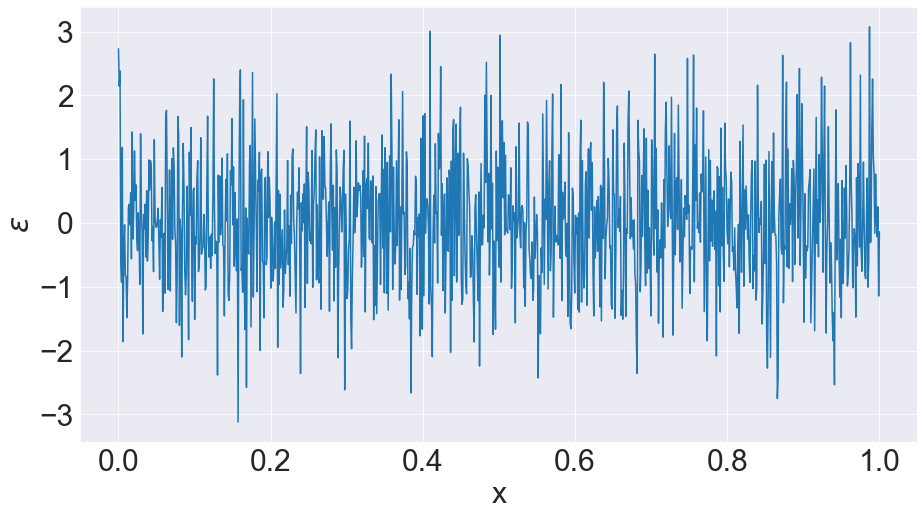
Figure 1: Homocedastic residuals.

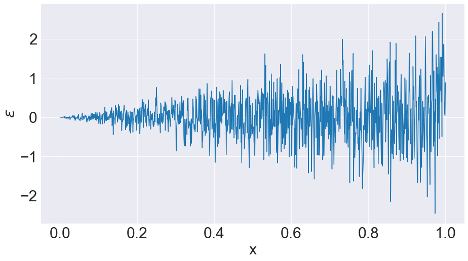
Figure 2: Heteroscedastic residuals.

1.3 Quantile regression

Usually, in a regression problem, we attempt to find the parameters $\bm{\theta}$ of a model $f_{\bm{\theta}}:\mathbb{R}^{D}\rightarrow\mathbb{R}$ via the minimization of the sum of squared residuals on the training set $\mathcal{D}_{train}$ as

$$\min_{\bm{\theta}}\sum_{i=1}^{n_{train}}(f_{\bm{\theta}}(\bm{x_{i}})-y_{i})^{2}+\Omega(\bm{\theta}),$$ (6)

where $\Omega(\bm{\theta})$ is a potential regularizer.

QR [9, 10], however, is a non-parametric method that attempts to approximate the true $\tau\in(0,1)$ conditional quantile $Q_{\tau}(\bm{x})$ given by

$$Q_{\tau}(\bm{x})=\inf{\{y\in\mathcal{Y}:F_{Y|\bm{X}}(y|\bm{X}=\bm{x})\geq\tau}\},$$ (7)

of the true conditional distribution $Y|\bm{X}$ by minimizing the following objective

$$\min_{\bm{\theta}}\sum_{i=1}^{n_{train}}\rho_{\tau}(y_{i},f_{\bm{\theta}}(\bm{x_{i}}))+\Omega(\bm{\theta}),$$ (8)

where $\rho_{\alpha}$ is the quantile loss, also known as pinball loss due to its resemblance to a pinball ball movement, see Fig.(3). This loss function can be mathematically expressed as

$$\rho_{\tau}(y,f_{\bm{\theta}}(\bm{x}))=\max\left(\tau(y-f_{\bm{\theta}}(\bm{x})),(\tau-1)(y-f_{\bm{\theta}}(\bm{x})\right).$$ (9)

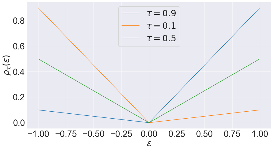
Figure 3: Visualization of the pinball loss where $\epsilon=y-f_{\bm{\theta}}(\bm{x})$ for different values of $\alpha$.

Consequently, it is suggested to train a QR model $f_{\bm{\theta}}(\bm{x})$ for $\tau=\alpha/2$ and $\tau=1-\alpha/2$ on $\mathcal{D}_{train}$ to obtain $1-\alpha$ conditional coverage via

$$[\hat{Q}_{\frac{\alpha}{2}}(\bm{x_{val}}),\hat{Q}_{1-\frac{\alpha}{2}}(\bm{x_{val})}],$$ (10)

where $\hat{Q}_{\frac{\alpha}{2}}(\bm{x_{val}})$ and $\hat{Q}_{1-\frac{\alpha}{2}}(\bm{x_{val}})$ are conditional quantile estimations of $Q_{\frac{\alpha}{2}}(\bm{x_{val}})$ and $Q_{1-\frac{\alpha}{2}}(\bm{x_{val}})$, respectively. Note that, unlike naive PIs, QR PIs are adaptive (they depend on the input). Another great virtue of QR is that it can be applied on top of any model by just changing the loss function to a pinball loss. Although the estimation $\hat{Q}_{\alpha}(\bm{x})$ yielded by QR of the unknown true conditional quantile $Q_{\alpha}(\bm{x})$ is known to be asymptotically consistent under certain conditions [7, 11, 12], it rarely provides $1-\alpha$ coverage in finite samples. To overcome this limitation, (Romano et al., 2019) [7] drawn several ideas from CP and devised the so-called CQR that we introduce in the next section.

2 Conformalized quantile regression

CQR grounds on correcting QR intervals with ICP techniques on a calibration set $\mathcal{D}_{cal}$ to ensure marginal coverage, hence inheriting the advantages of both, i.e., adaptive intervals with marginal coverage guarantee. Specifically, if QR bounds are constantly undercovering, then PIs must get wider. On the contrary, in case of QR PIs cover in a ratio superior to $1-\alpha$, they must be shortened. For this purpose, (Romano et al., 2019) [7] proposed the following non-conformity score function

$$s(\bm{x},y)=\max{\{\hat{Q}_{\frac{\alpha}{2}}(\bm{x})-y,y-\hat{Q}_{1-\frac{\alpha}{2}}(\bm{x})\}}.$$ (11)

Subsequently, after calculating $\hat{q}=\text{Quantile}(\bm{\epsilon};1-\alpha)$, adaptive PIs with $1-\alpha$ marginal coverage guarantee are yielded as

$$[\hat{Q}_{\frac{\alpha}{2}}(\bm{x_{val}})-\hat{q},\hat{Q}_{1-\frac{\alpha}{2}}(\bm{x_{val}})+\hat{q}]$$ (12)

Built on the same idea, a different non-conformity score function was proposed in [13]; however, it has not proved to outperform the non-conformity score function in Eq.(11) [14]. Note that, a $\hat{q}>0$ (most cases) is a result of a QR model that did not ensure $1-\alpha$ coverage and therefore PIs must get wider. In the case of $\hat{q}<0$, it signifies that QR bounds are overcovering and thus we shoul narrow the bounds, i.e., the lower bound increases $\hat{q}$ units and the upper bound decreases the same amount, while still ensuring $1-\alpha$ marginal coverage.

CQR seems appealing, and it is in fact, yet the calibration step lacks adaptiveness. The role of $\hat{q}$ is to simply shift the bounds $\hat{q}$ units. Also, it does not depend on the input at hand in any form. Our contribution, presented in the next section, will focus on improving the calibration step to make it more adaptive and dependent on the input. However, this improvement is only possible in tabular data.

3 Contribution

Our idea to improve CQR is to do k conformal steps instead, one per each group, as illustrated in Fig.(4). This is based on the idea that $\bm{x_{1}}\approx\bm{x_{2}}\implies f_{\bm{\theta}}(\bm{x_{1}})\approx f_{\bm{\theta}}(\bm{x_{2}})$. To attain such goal, we could compute the euclidean distance between observations and cluster them using K-means [15]; however, this is not a good heuristic to approximate the conditional distribution $Y|X$. We need two additional conditions: (1) features must be scaled, since euclidean distance is scale-dependent; and (2) each feature has a different predictive power upon the response variable y. To accommodate condition (2), whenever clustering the observations, we must weigh each feature by the respective feature importance. A simple way of calculating feature importance that work for any model is permutation importance [16]. Algorithms (1), (2), and (3) comprise every step to successfully perform K-means, permutation importance, and our improved CQR version, respectively. In a nutshell, these are the main steps of our improved version: (1) normalize the training data, and apply the same normalization object on the calibration and validation set; (2) train $f_{\bm{\theta}}:\mathbb{R}^{D}\rightarrow\mathbb{R}$ with pinball loss for $\tau=\frac{\alpha}{2}$ and $\tau=1-\frac{\alpha}{2}$; (3) get feature importance by means of permutation importance algorithm using the calibration set for evaluation; (4) create a copy of the training set, calibration set, and validation set weighted by feature importance, henceforth referred to as clustering training set, clustering calibration set, and clustering validation set, respectively; (5) select the best k of K-means on the clustering calibration set and store k centroids to represent each cluster; (6) assign each observation of the clustering calibration set to the nearest cluster/centroid; (7) knowing which elements belong to each of the k clusters given by the previous step, compute a different $\hat{q}$ for each cluster using Eq.(11) as the non-conformity score function on the calibration set; (8) given a new observation $\bm{x_{val}}$, find the nearest centroid $\bm{c_{i}}$ of $\bm{x_{val}^{*}}$ (the matching observation of $x_{val}$ weighted by the respective permutation importance.) and use the respective $\hat{q}^{(i)}$ to produce PIs as $[\hat{Q}_{\frac{\alpha}{2}}(\bm{x_{val}})-\hat{q}^{(i)},\hat{Q}_{1-\frac{\alpha}{2}}(\bm{x_{val}})+\hat{q}^{(i)}]$.

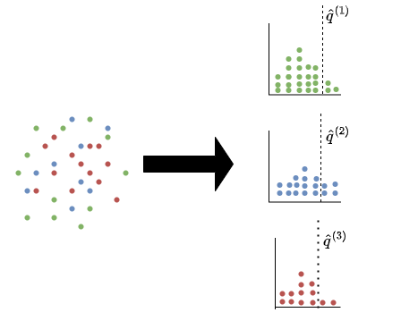
Figure 4: Group-balanced conformal prediction. Image inspired by [17].

K-means, as shown in Algorithm (1) is a clustering algorithm that attempts to minimize the following objective

$$L=\sum_{i=1}^{k}\sum_{\bm{x}\in S_{i}}||\bm{x}-\bm{c_{i}}||^{2},$$ (13)

where k is the number of clusters; $S_{i}$ denotes the cluster set i; $c_{i}$ the centroid of cluster i; and $||.||$ the euclidean norm.

Since K-means relies upon the hyperparameter k to define the number of clusters beforehand, we must select a criteria to find the potential best k. For the purpose at hand, the fraction of variance explained by the centroids is a good choice, which is mathematically expressed as

$$\sigma_{k}=\frac{\sum_{i=1}^{k}n_{i}(\bm{c_{i}}-\bm{\mu})^{T}(\bm{c_{i}}-\bm{\mu})}{\sum_{i=1}^{N}(\bm{x_{i}}-\bm{\mu})^{T}(\bm{x_{i}}-\bm{\mu})},$$ (14)

where $n_{i}$ is the number of examples in cluster i and $\bm{\mu}$ denotes the feature mean.

Remarks

• The selection of k for K-means is not limited to our approach, different criteria regarding the selection of k for K-means are acceptable, e.g., silhouete score and elbow method [18, 19, 20];

• Different clustering algorithms beyond K-means might also be adequate as long as they take in consideration the essential point, which is cluster based on similarity between observations and feature importance.

Algorithm 1 K-means algorithm

1:$\bm{c_{1}}^{(1)},\bm{c_{2}}^{(1)},...,\bm{c_{k}}^{(1)}$ initial centroids efficiently randomly assigned as in [21].

2:k clusters given by their centroids that minimize Eq.(13)

3:Converged $\leftarrow$ False

4:$t\leftarrow 1$

5:while Converged is False do

6:     Assign each observation to the cluster with the nearest centroid i given by

7:     $S_{i}^{(t)}=\{\bm{x}:||\bm{x}-\bm{c_{i}}^{(t)}||\leq||\bm{x}-\bm{c_{j}}^{(t)}||\;\forall 1\leq j\leq k\}$

8:     $t\leftarrow t+1$

9:     Update centroids

10:     for $i\leftarrow 1$ to k do

11:         $\bm{c_{i}}^{(t+1)}\leftarrow\frac{1}{|S_{i}^{(t)}|}\sum_{\bm{x}\in S_{i}^{(t)}}\bm{x}$

12:     end for

13:     Stop if all clusters are the same as from previous iteration.

14:     if $\bm{c_{i}}^{(t+1)}=\bm{c_{i}}^{(t)},\quad\forall i\in\{1,2,...,k\}$ then

15:         Converged $\leftarrow$ True

16:     end if

17:end while

Algorithm 2 Permutation importance

1:A dataset $\mathcal{D}$=$\{(\bm{x_{i}},y_{i})\}_{i=1}^{N}$, a model $f_{\bm{\theta}}:\mathbb{R}^{D}\rightarrow\mathbb{R}$, a performance measure M, and R repetitions.

2:D feature importance’s $I_{1},I_{2},...,I_{D}$

3:Split $\mathcal{D}$ in two mutually exclusive sets, a training set $\mathcal{D}_{train}=(X_{train},\bm{y_{train}})$ and a validation set $\mathcal{D}_{val}=(X_{val},\bm{y_{val}})$

4:Train $f_{\bm{\theta}}$ on $\mathcal{D}_{train}$, and compute the baseline error score $E_{b}$ on $\mathcal{D}_{val}$ using the performance measure M

5:for $j\leftarrow 1$ to D do

6:     for $i\leftarrow 1$ to R do

7:         Permutate column j on the validation X set $X_{val}$ and compute the permutated error score $E_{\pi_{j}}^{(i)}$ using performance measure M

8:         $\Delta_{j}^{(i)}\leftarrow|E_{b}-E_{\pi_{j}}^{(i)}|$

9:     end for

10:     $I_{j}\leftarrow\frac{1}{R}\sum_{i=1}^{R}\Delta_{j}^{(i)}$

11:end for

Algorithm 3 Improved conformalized quantile regression (ICQR)

1:Three normalized sets: $\mathcal{D}_{train}=(X_{train},\bm{y_{train}}),\mathcal{D}_{cal}=(X_{cal},\bm{y_{cal}})$, and $\mathcal{D}_{val}=(X_{val},\bm{y_{val}})$, miscoverage error rate $\alpha$, desired explained variance $\sigma$, maximum number of clusters K, R repetitions, and a model $f_{\bm{\theta}}:\mathbb{R}^{D}\rightarrow\mathbb{R}$

2:Adaptive intervals with $1-\alpha$ coverage

3:Part 1: Estimate conditional quantiles with quantile regression.

4:

5:Use QR to estimate $\hat{Q}_{\frac{\alpha}{2}}(\bm{x})$ and $\hat{Q}_{1-\frac{\alpha}{2}}(\bm{x})$ on $\mathcal{D}_{train}$.

6:

7:Part 2: Weigh the X sets by the feature importance of each feature $I_{1},I_{2},...,I_{D}$.

8:

9:Get a list of feature importances $I_{1},I_{2},...,I_{D}$ given by Algorithm (2) using $\mathcal{D}_{cal}$ for evaluation.

10:$X_{cal}^{*},X_{val}^{*}\leftarrow 0_{n_{cal}\times D},0_{n_{val}\times D}$

11:for $i\leftarrow 1$ to D do

12:     col${}_{i}(X_{cal}^{*})\leftarrow$col${}_{i}(X_{cal})\times I_{i}$

13:     col${}_{i}(X_{val}^{*})\leftarrow$col${}_{i}(X_{val})\times I_{i}$

14:end for

15:

16:Part 3: Selection of k for K-means.

17:

18:$k\leftarrow 2$

19:$best_{k}\leftarrow$ False

20:while $k\leq K$ and $best_{k}$ is False do

21:     Apply K-means as in Algorithm (1) on $X_{cal}^{*}$.

22:     Compute $\sigma_{k}$ as in Eq.(14).

23:     if $\sigma_{k}>\sigma$ then

24:         $best_{k}\leftarrow$ True

25:         Store the cluster centroids $\bm{c_{1}},\bm{c_{2}},...,\bm{c_{k}}$

26:     else

27:         $k\leftarrow k+1$

28:     end if

29:end while

30:

31:Part 4: Compute $\hat{q}^{(1)},\hat{q}^{(2)},...,\hat{q}^{(k)}$ on the calibration set, one per cluster.

32:

33:$\bm{\epsilon}^{(1)},\bm{\epsilon}^{(2)},...,\bm{\epsilon}^{(k)}\leftarrow\{\},\{\},....,\{\}$

34:for $(\bm{x^{*}},\bm{x},y)$ in $(X_{cal}^{*},X_{cal},\bm{y_{cal}})$ do

35:     $i\leftarrow\operatorname*{\arg\!\min}_{j\in\{1,2,...,k\}}{||\bm{x^{*}}-\bm{c_{j}}||}$

36:     $\bm{\epsilon}^{(i)}\leftarrow\bm{\epsilon}^{(i)}\cup\left\{\max\left(\hat{Q}_{\frac{\alpha}{2}}(\bm{x})-y,y-\hat{Q}_{1-\frac{\alpha}{2}}(\bm{x})\right)\right\}$

37:end for

38:$\hat{q}^{(i)}\leftarrow\text{Quantile}\left(\bm{\epsilon}^{(i)};1-\alpha\right),\quad\forall i\in\{1,...,k\}$

39:

40:Part 5: Deploy PIs on new data. Exemplified as $(X_{val},\bm{y_{val}})$.

41:

42:for $(\bm{x^{*}},\bm{x},y)$ in $(X_{val}^{*},X_{val},\bm{y_{val}})$ do

43:     $i\leftarrow\operatorname*{\arg\!\min}_{j\in\{1,2,...,k\}}{||\bm{x^{*}}-\bm{c_{j}}||}$

44:     Return $\hat{C}_{1-\alpha}(\bm{x})\leftarrow[\hat{Q}_{\frac{\alpha}{2}}(\bm{x})-\hat{q}^{(i)},\hat{Q}_{1-\frac{\alpha}{2}}(\bm{x})+\hat{q}^{(i)}]$

45:end for

4 Experiments

In this section we apply Algorithm (3) and compare it against CQR, QR and Naive on the datasets shown in Table (2). We use a FFNN (feedforward neural network) [22] with two output neurons to estimate $Q_{\frac{\alpha}{2}}(\bm{x})$, and $Q_{1-\frac{\alpha}{2}}(\bm{x})$, respectively. This is easily achieved by having a pinball loss function with $\tau=\alpha/2$ for the first output neuron and $\tau=1-\alpha/2$ for the second. $\hat{Q}_{\frac{\alpha}{2}}(\bm{x})$ and $\hat{Q}_{1-\frac{\alpha}{2}}(\bm{x})$ represent the estimated lower bound, upper bound, with respect to $\bm{x}$, respectively. Due to the stochastic behaviour of FFNN, the model is trained T=100 times to reduce the associated variance of the random initialization. On top of these 100 trained models each of the aforementioned methods is applied. Each dataset in Table (2) is divided in three mutually exclusive datasets, a training set containing 50% of the data, a calibration set with 25%, and a evaluation set with the last 25%. Thereafter, each method is assessed on the evaluation set considering summary statistics of PIs width and coverage for $\alpha=0.1$ and a threshold explained variance of $\sigma_{k}=0.9$. All the data and code, which is written in Python can be found here.

Dataset	N	D	Source
Blogfeedback	60.000	280	[23]
Boston house prices	506	13	[24]
Bike sharing	17379	17	[25]

Table 2: Datasets description.

Blogfeedback

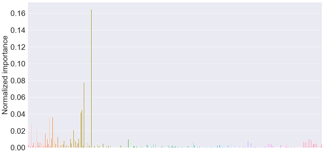
(a)

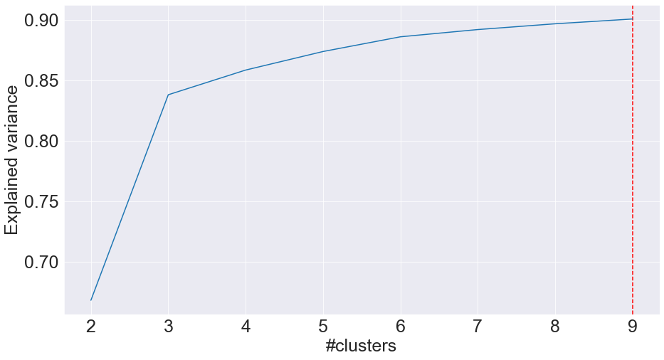
(b)

Figure 5: (Blogfeedback) Feature importance (panel left). Number of clusters for a threshold fraction variance of 0.9 (panel right).

Method	min	max	mean	std	Q1	median	Q3	IQR
Naive	14.943970	20.984375	17.479034	0.976794	16.812687	17.417236	18.004509	1.191822
QR	0.000002	1546.067383	5.822205	17.578970	1.105402	2.070409	4.677099	3.571697
CQR	0.054895	1552.663086	12.865065	17.589760	8.126973	9.508371	12.118934	3.991961
ICQR	0.000061	1595.305754	23.701899	47.737405	2.431001	5.260328	35.063214	32.632213

Table 3: (Blogfeedback) PI width summary statistics.

Method	min	max	mean	std	Q1	median	Q3	IQR
Naive	0.899440	0.908237	0.903714	0.001837	0.902656	0.903872	0.904788	0.002132
QR	0.332600	0.828469	0.747061	0.092558	0.745585	0.778722	0.792366	0.046781
CQR	0.897908	0.906837	0.902400	0.002016	0.900756	0.902306	0.904105	0.003349
ICQR	0.894775	0.906371	0.901395	0.002302	0.899907	0.901706	0.902972	0.003065

Table 4: (Blogfeedback) Coverage summary statistics.

Boston house prices

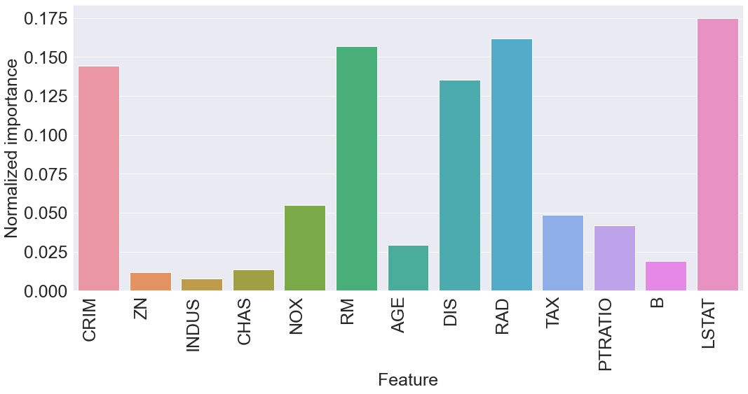
(a)

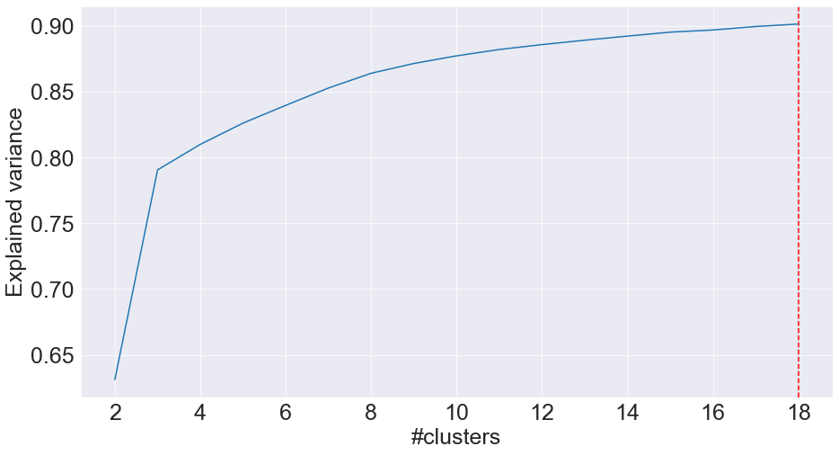
(b)

Figure 6: (Boston house prices) Feature importance (panel left). Number of clusters for a threshold fraction variance of 0.9 (panel right).

Method	min	max	mean	std	Q1	median	Q3	IQR
Naive	9.530071	12.689045	10.898064	0.602834	10.478755	10.807868	11.260028	0.781272
QR	1.324307	32.966770	8.323204	2.736615	6.490421	7.689121	9.650486	3.160065
CQR	2.978894	36.200993	10.921992	2.769641	9.070092	10.472181	12.346348	3.276256
ICQR	1.812310	44.346356	12.020735	4.937976	8.044880	10.293163	15.649653	7.604772

Table 5: (Boston house prices) PI width summary statistics.

Method	min	max	mean	std	Q1	median	Q3	IQR
Naive	0.889764	0.976378	0.940472	0.018104	0.929134	0.944882	0.952756	0.023622
QR	0.771654	0.889764	0.837795	0.025148	0.818898	0.834646	0.858268	0.039370
CQR	0.866142	0.984252	0.938583	0.020290	0.929134	0.937008	0.952756	0.023622
ICQR	0.889764	0.984252	0.943228	0.019489	0.929134	0.944882	0.960630	0.031496

Table 6: (Boston house prices) Coverage summary statistics.

Bike sharing

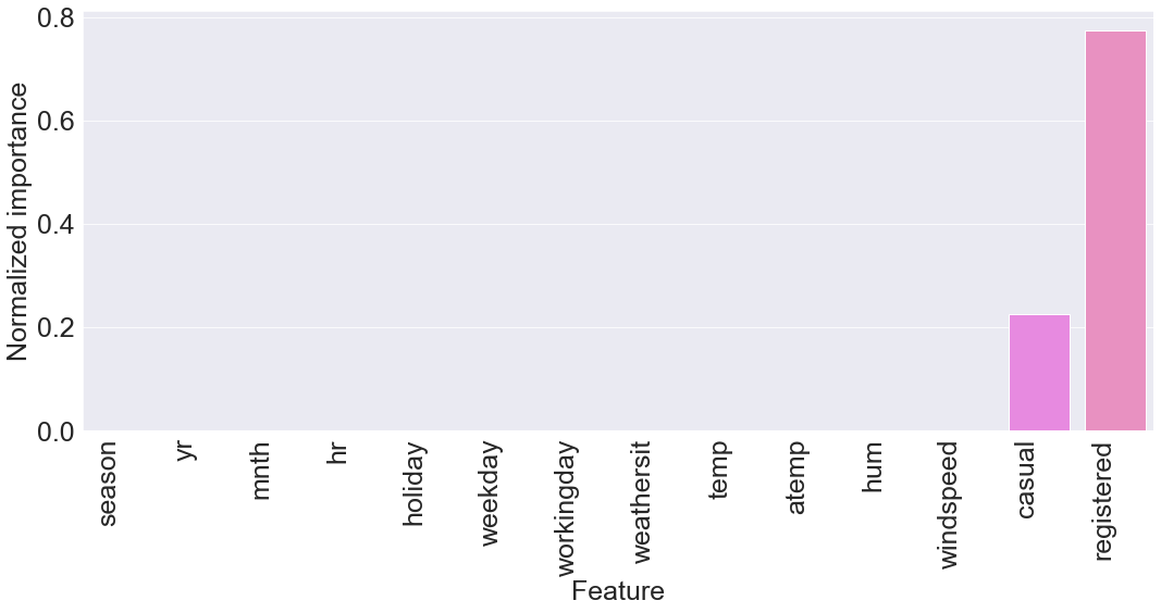
(a)

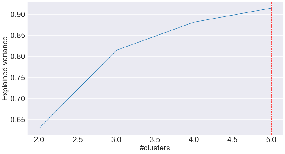
(b)

Figure 7: (Bike sharing) Feature importance (panel left). Number of clusters for a threshold fraction variance of 0.9 (panel right).

Method	min	max	mean	std	Q1	median	Q3	IQR
Naive	0.427124	7.491333	2.336785	1.362940	1.327354	2.135223	3.189590	1.862236
QR	0.001831	35.566101	3.324998	2.115591	2.047175	2.682456	3.896203	1.849028
CQR	0.000229	36.159119	2.763314	2.186563	1.385670	2.202379	3.450058	2.064388
ICQR	0.000165	25.988984	2.249955	1.470346	1.267076	1.949806	2.848970	1.581894

Table 7: (Bike sharing) PI width summary statistics.

Method	min	max	mean	std	Q1	median	Q3	IQR
Naive	0.891139	0.915535	0.900700	0.004449	0.897583	0.900575	0.903625	0.006041
QR	0.084695	1.000000	0.897445	0.193131	0.887687	0.987457	0.995224	0.107537
CQR	0.887227	0.910702	0.900242	0.005158	0.897756	0.900230	0.904028	0.006272
ICQR	0.889068	0.916686	0.902656	0.006272	0.897986	0.902762	0.906847	0.008861

Table 8: (Bike sharing) coverage summary statistics.

Results discussion

In the two first datasets, QR is constantly undercovering; hence, QR bounds are in need of ICP to ensure $1-\alpha$ coverage. ICQR is clearly more adaptive to heteroscedasticity in comparison to CQR since it has generally higher std and IQR PI width, but lower median PI width, while still ensuring the same coverage, as seen in Table (3-6).

In the last dataset (bike sharing), we have the opposite case, QR is overcovering as seen in Table (8). Consequently, we can reduce the bounds up to $1-\alpha$ coverage with ICP.

Remarks

• Naive bounds are not dependent on the input in any form nor adaptive. The interval amplitude is always equal to $2\hat{q}$. The small deviation seen in the above tables is a result of training the model 100 times to reduce the variance associated with FFNN due to the random initialization process.

• Evaluating PIs by just looking to their mean value is not adequate. Most times, naive method has the lowest mean value; however, it achieves $1-\alpha$ coverage not in a group-balanced way, overcovering easy inputs, and PIs have always the same amplitude, ignoring heteroscedasticity. Therefore, analyzing PIs width by quantile gives a better perspective regarding conditional coverage. Adaptive methods generally have higher mean PI width because they are not optimized for heteroscedastic residuals. Nevertheless, the median PI width is usually lower in adaptive/heteroscedastic methods.

5 Conclusion

In this paper, we have proposed an improved version of CQR. Results demonstrate that our version is further adaptive to heteroscedasticity, hence ICQR is one step ahead towards conditional coverage. The major shortcoming of ICQR in comparison to CQR are the two additional steps to calculate permutation importance and perform K-means. Despite this minor disadvantage, ICQR offers eye-catching adaptive PIs in comparison to the classic CQR, which convey us to strongly endorse its use across any high-stakes tabular regression problem.

References

- [1] Ethan Goan and Clinton Fookes. Bayesian neural networks: An introduction and survey. In Case Studies in Applied Bayesian Data Science, pages 45–87. Springer International Publishing, 2020.
- [2] David M. Blei, Alp Kucukelbir, and Jon D. McAuliffe. Variational inference: A review for statisticians. Journal of the American Statistical Association, 112(518):859–877, apr 2017.
- [3] Charles Blundell, Julien Cornebise, Koray Kavukcuoglu, and Daan Wierstra. Weight uncertainty in neural network. In Francis Bach and David Blei, editors, Proceedings of the 32nd International Conference on Machine Learning, volume 37 of Proceedings of Machine Learning Research, pages 1613–1622, Lille, France, 07–09 Jul 2015. PMLR.
- [4] Tom Heskes. Practical confidence and prediction intervals. In Proceedings of the 9th International Conference on Neural Information Processing Systems, NIPS’96, page 176–182, Cambridge, MA, USA, 1996. MIT Press.
- [5] Yarin Gal and Zoubin Ghahramani. Dropout as a bayesian approximation: Representing model uncertainty in deep learning. In international conference on machine learning, pages 1050–1059. PMLR, 2016.
- [6] Vladimir Vovk, Alexander Gammerman, and Glenn Shafer. Algorithmic learning in a random world. 2005.
- [7] Yaniv Romano, Evan Patterson, and Emmanuel Candes. Conformalized quantile regression. In H. Wallach, H. Larochelle, A. Beygelzimer, F. d'Alché-Buc, E. Fox, and R. Garnett, editors, Advances in Neural Information Processing Systems, volume 32. Curran Associates, Inc., 2019.
- [8] Arun Kumar Kuchibhotla. Exchangeability, conformal prediction, and rank tests, 2020.
- [9] Roger Koenker and Kevin F Hallock. Quantile regression. Journal of economic perspectives, 15(4):143–156, 2001.
- [10] Roger W Koenker and Gilbert Bassett. Regression quantiles. Econometrica, 46(1):33–50, 1978.
- [11] Ichiro Takeuchi, Quoc Le, Timothy Sears, and Alexander Smola. Nonparametric quantile estimation. Journal of Machine Learning Research, 7:1231–1264, 12 2006.
- [12] Ingo Steinwart and Andreas Christmann. Estimating conditional quantiles with the help of the pinball loss. Bernoulli, 17(1), feb 2011.
- [13] Danijel Kivaranovic, Kory D. Johnson, and Hannes Leeb. Adaptive, distribution-free prediction intervals for deep networks, 2019.
- [14] Matteo Sesia and Emmanuel J. Candè s. A comparison of some conformal quantile regression methods. Stat, 9(1), jan 2020.
- [15] Kardi Teknomo. K-means clustering tutorial. Medicine, 100(4):3, 2006.
- [16] André Altmann, Laura Toloşi, Oliver Sander, and Thomas Lengauer. Permutation importance: a corrected feature importance measure. Bioinformatics, 26(10):1340–1347, 2010.
- [17] Anastasios N. Angelopoulos and Stephen Bates. A gentle introduction to conformal prediction and distribution-free uncertainty quantification, 2021.
- [18] Fei Wang, Hector-Hugo Franco-Penya, John D Kelleher, John Pugh, and Robert Ross. An analysis of the application of simplified silhouette to the evaluation of k-means clustering validity. In International Conference on Machine Learning and Data Mining in Pattern Recognition, pages 291–305. Springer, 2017.
- [19] Purnima Bholowalia and Arvind Kumar. Ebk-means: A clustering technique based on elbow method and k-means in wsn. International Journal of Computer Applications, 105(9), 2014.
- [20] D. Pham, Stefan Dimov, and Cuong Nguyen. Selection of k in k -means clustering. Proceedings of The Institution of Mechanical Engineers Part C-journal of Mechanical Engineering Science - PROC INST MECH ENG C-J MECH E, 219:103–119, 01 2005.
- [21] David Arthur and Sergei Vassilvitskii. k-means++: The advantages of careful seeding. Technical report, Stanford, 2006.
- [22] Daniel Svozil, Vladimir Kvasnicka, and Jiri Pospichal. Introduction to multi-layer feed-forward neural networks. Chemometrics and Intelligent Laboratory Systems, 39(1):43–62, 1997.
- [23] Blogfeedback dataset. https://archive.ics.uci.edu/ml/datasets/BlogFeedback. Accessed: 2022-07-5.
- [24] Boston house prices dataset. https://www.kaggle.com/datasets/vikrishnan/boston-house-prices. Accessed: 2022-07-5.
- [25] Bike sharing dataset. https://archive.ics.uci.edu/ml/datasets/bike+sharing+dataset. Accessed: 2022-07-5.