Computational fluid dynamics approach
for understanding oscillating and interacting convective flows

Abstract

A 2D numerical hydrodynamics approach is considered for modelling recent experimental results on the oscillation and collective behavior of convective flows. Our simulations consider the rising dynamics of heated fluid columns in a gravitational field. Simulations are done on two entirely different length-scales, showing also the generality of the investigated phenomena. For the flow of a single heated fluid column, the effect of the inflow yield and the nozzle diameter is studied. In agreement with the experiments, for a constant nozzle diameter the oscillation frequency increases approximately linearly as a function of the the flow yield and for a constant flow yield the frequency decreases as a power law with the increasing nozzle diameter. Concerning the collective behavior of two nearby flow we find a counter-phase synchronization of the oscillations and an increasing trend in the common oscillation frequency when the distance between the flows is decreased. These results are again in agreement with the experimental findings.

I Introduction

Recent experimental results have proven that rising gas columns can perform oscillations and their interaction leads to fascinating collective behavior Gergely et al. (2021). These oscillations have been reported much earlier by Yuan et. al Yuan, Durox, and Villermaux (1994) and can be discussed in analogy with the very similar phenomena known for diffusive flames Chamberlin and Rose (1948); Durox et al. (1995); Durox, Yuan, and Villermaux (1997); Huang et al. (1999); Kitahata et al. (2009); Ghosh et al. (2010); Okamoto et al. (2016); Chen et al. (2019); Gergely et al. (2020). The toy-model presented in Gergely et al. (2021) is clearly inadequate to explain the fine details observed in our recent experiments, therefore a more sophisticated theoretical approach is needed. The present study contributes in this sense, considering a 2D numerical hydrodynamics approach to this phenomenon.

For validating the numerical results, the present work considers as reference the experiments realized using a controlled flow of Helium into air Gergely et al. (2021) . In these experiments the Schlieren technique Settles (2001); Leptuch and Agrawal (2006) was used to visualize the flow, allowing also a digital processing of the oscillations. From the images processed by the Otsu method Otsu (1979); FreddyCree (2020) the characteristic frequency and the relevant synchronization order parameter was derived. For a better understanding of the phenomena, some sample movies with original recordings and the ones processed with the Otsu method are given in our YouTube channel Gergely (2020a). For a single flow column the experiments investigated the effect of the nozzle diameter and flow rate on the observed oscillation frequency. For the collective behavior of two nearby flows the experiments described in Gergely et al. (2021) investigated the phase difference between the oscillations, their frequency and a proper synchronization order parameter as a function of the separation distance between the flows. It was concluded that at a constant Helium flow yield the oscillation frequency of the rising gas column decreases in from of a power law as a function of the nozzle diameter. This finding is similar with the observed oscillation frequency of the flames of candle bundles as a function of the number of candles in the bundle Gergely et al. (2020). For a constant nozzle diameter it was found that the oscillation frequency of the flow increases linearly with the flow yield. For the collective behavior of two nearby and clearly separated flow columns with similar flow parameters only counter-phase synchronization was observed. This is somehow different from the phenomena observed for candle bundle flames, where both in-phase and counter phase synchronization is present depending on the distance between the flames Gergely et al. (2020). The experiments concluded that for short distances the oscillation frequency of the flow column becomes significantly higher than the frequency observed for non-interacting Helium columns with the same parameters (flow rate and nozzle diameter). All the above summarized results, should be a test for any numerical simulation approach on this interesting phenomenon.

Due to the complexity of the problems related to flows in different spatial configurations, computation approaches are many times the only theoretical possibilities to realistically model such phenomena (see for example Joel H. Ferziger and Street (2020); Wendt (2009)). Even with such a modelling methodology, imposing the right boundary conditions and offering a proper discretization of space and time raises many technical challenges V. Venkatakrishnan and R. Chakravarthy (1998). The incredible revolution we experience nowadays in computational resources and methods, helped us to overcome much of these difficulties and computational fluid dynamics became the primary tool to investigate theoretically problems related to fluid dynamics. However, even with the presently available computational power, many times we are forced to investigate a simpler flow topology and reduce the dimensionality of the problem Correa et al. (2019). This is nowadays a standard procedure for those cases where the problem becomes computationally difficult in 3D. Usually a two-dimensional simplification is considered when the periodicity and symmetry of the considered flow allows this. Assuming in the followings a cylindrical symmetry for the flow, we consider a two-dimensional numerical fluid dynamics approach to the above described phenomenon. First, we discuss the theoretical background on which our approach is build and the details of the applied numerical method. Using simple and straightforward examples we test the simulation environment and gain confidence in the method. After this methodological part, we approach the proposed problem and compare critically the results of the simulations with the experimental data from Gergely et al. (2021). Finally, conclusions are drown and universality features of this intriguing phenomenon is discussed.

II The numerical approach

We present here a 2D numerical approach, that is suitable for modelling the oscillations and collective behavior observed in rising gas columns. In order to further simplify the problem, instead of a Helium column injected from the bottom we consider the flow of the same incompressible fluid as the surrounding, heated in a restricted region at the bottom of the simulated area. In such manner we get a rising gas column which is also realizable in experiments.

Using the same Schlieren technique as before, on Figure 1 and on the movies presented in Gergely (2020b) we show that very similar instabilities and oscillations occur. In these kitchen-experiments the heating is realized by a simple heating coil in which one controls the dissipated electric power. Unfortunately in such experiments there is no good control over the flow debit, therefore one cannot conduct such carefully monitored experiments as were done for Helium. This is the main reason why the numerical results are compared with our earlier experiments presented in Gergely et al. (2021).

The advantage of the proposed setup is that we do not have to apply the numerical fluid dynamics method for two component gases. We pay however for this simplification by the non-homogeneous temperature field, therefore extra transports and gradients has to be taken into account.

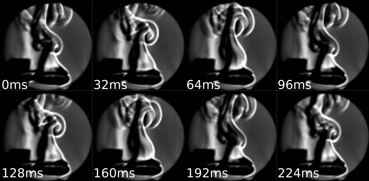
Figure 1: Visualization of a rising hot-air column by the Schlieren technique. Similar instabilities and oscillations appear as in the case of the rising Helium gas column.

In our approach the fluid is considered to be an ideal one described by the Navier-Stokes equation. For an incompressible fluid in a gravitational field, the Navier-Stokes equation writes in the following form:

$$\begin{split}\rho\cdot\frac{\partial\mathbf{u}}{\partial t}+\rho\cdot\left(\mathbf{u}\cdot\nabla\right)\cdot\mathbf{u}&=-\nabla p+\mathbf{g}\cdot\rho+\mu\cdot\Delta\mathbf{u}\\ \nabla\mathbf{u}&=0\end{split}$$ (1)

Here $\rho$ denotes the density, $p$ is the pressure, $\mathbf{g}$ the gravitational acceleration, $\mathbf{u}$ is the velocity of the fluid, and $\mu$ denotes the fluid’s viscosity. The quantities $\mathbf{u}$ and $p$ can be time and position dependent in the flow-space.

For the considered problem, the convective flow due to the temperature difference plays a key role, therefore in the Navier-Stokes equation, we have to take into account the temperature dependence of the density and describe also the time evolution of the temperature inside the fluid. The evolution of temperature and the temperature dependence of the density, are considered by the following equations:

$$\begin{split}\rho=\frac{\rho_{0}}{1+(T-T_{0})\cdot\alpha}\\ \frac{\partial T}{\partial t}=D\cdot\Delta T-(\mathbf{u}\cdot\nabla)\cdot T\end{split}$$ (2)

In the above equations, $\rho_{0}$ is the density at $T_{0}$, $T$ is the temperature of the fluid at a given spatial position and in a given time-moment, $D$ is the diffusion constant and $T_{0}$ is the ambient temperature. The numerical solution of the coupled systems of partial differential equations (1)-(2) was done by using the "FEniCS" software package Langtangen and Logg (2017). FEniCS is an open-source platform developed for solving Partial Differential Equation (PDE) systems. We chose this platform because it has high-level programming interfaces (C ++, Python), the shape of the equations in the program code is similar to their symbolic form and the program is optimized for a wide range of hardware from laptops to high-performance clusters.

II.1 The simulation code

FEniCS uses finite element methods to solve PDEs. As an example in Appendix A we illustrate how to solve the simple 2D Poison equation with FEniCS. For our specific problem we first deal with the term describing the evolution of temperature:

$$\begin{split}\frac{\partial T}{\partial t}=D\cdot\Delta T-(\mathbf{u}\cdot\nabla)\cdot T\end{split}$$ (3)

This equation contains a time derivative, so in addition to the coordinates we also have to discretize time. This is done by the Euler method as follows:

$$\begin{split}\frac{T(t+dt)-T(t)}{dt}=D\cdot\Delta T(t)-(\mathbf{u}\cdot\nabla)\cdot T(t),\end{split}$$ (4)

where the indexes for the $T$ temperature label the discretized time-steps. We then bring each term to the left hand side of the equation, we multiply the equation by a $\tau$ test function, and integrate the equation over the entire simulated domain:

$$\int_{\Omega}[T(t+dt)-T(t)-D\cdot\Delta T(t)\cdot dt+(\mathbf{u}\cdot\nabla)\cdot T(t)\cdot dt]\cdot\tau\ d\Omega=0$$ (5)

The equations from above contains a second-order derivative for the coordinates, which is eliminated by partial integration:

$$\int_{\Omega}(\nabla^{2}\cdot T(t))\cdot\tau\ d\Omega=\int_{\partial\Omega}\left(\frac{\partial T(t)}{\partial\mathbf{n}}\right)\cdot\tau\ ds-\int_{\Omega}\nabla T(t)\cdot\nabla\tau\ d\Omega$$ (6)

Here we denoted by $\mathbf{n}$ the unit normal vector to the $\partial\Omega$ surface. The derivative in respect to $\mathbf{n}$ is defined as:

$$\frac{\partial T}{\partial\mathbf{n}}=(\nabla T)\cdot\mathbf{n}$$ (7)

Rewriting equation (5) using the above result and the fact that under the Dirichlet and free boundary conditions the surface integral disappears, we obtain the final form:

$$\int_{\Omega}([T(t+dt)-T(t)+(\mathbf{u}\cdot\nabla)\cdot T(t)\cdot dt]\cdot\tau\ +D\cdot\nabla T(t)\cdot\nabla\tau\cdot dt\ )\,d\Omega=0$$ (8)

The incompressible Navier-Stokes equation (1) was solved using the IPCS (Incremental Pressure Correction Scheme) scheme Logg et al. (2012). The IPCS method consists of 3 steps but before specifying the steps we introduce the following functions and notation:

$$\begin{split}[\varepsilon(\mathbf{u})]=\frac{1}{2}\cdot([\nabla\otimes\mathbf{u}]+[\nabla\otimes\mathbf{u}]^{T})\\ [\sigma(\mathbf{u},p)]=2\cdot\mu\cdot\varepsilon(\mathbf{u})-p\cdot I\\ {\langle\mathbf{f},\mathbf{g}\rangle}_{\Omega}=\int_{\Omega}\mathbf{f}\cdot\mathbf{g}\ d\Omega\\ {\langle[A],[B]\rangle}_{\Omega}=\int_{\Omega}[A]:[B]\ d\Omega\end{split}$$ (9)

The $\otimes$ product is defining a matrix with the following elements:

$$\nabla\otimes\mathbf{u}=\left[\frac{\partial u_{j}}{\partial x_{i}}\right]$$ (10)

We denoted by $[...]$ a square matrix, by $[...]^{T}$ the transpose of a matrix and by $:$ the inner product of matrices:

$$[A]:[B]\equiv\sum_{i,j}A_{ij}\,B_{ij}$$ (11)

Using the $\varepsilon$ and $\sigma$ functions and the specified notation, the steps of the method will be described in the followings. First we reconsider the Navier-Stokes equation in a discretised form on the $\Omega$ velocity space:

$$\rho\cdot{\left\langle\frac{\mathbf{u}^{*}-\mathbf{u}(t)}{dt},\mathbf{v}\right\rangle}_{\Omega}+\rho\cdot{\left\langle\mathbf{u}(t)\cdot\nabla\mathbf{u}(t),\mathbf{v}\right\rangle}_{\Omega}+{\left\langle\left[\sigma\left(\frac{\mathbf{u}(t)+\mathbf{u}^{*}}{2},p(t)\right)\right],\left[\varepsilon(\mathbf{v})\right]\right\rangle}_{\Omega}+$$ (12)

$$+{\left\langle p(t)\cdot\mathbf{n},\mathbf{v}\right\rangle}_{\partial\Omega}-{\left\langle\mathbf{n}\cdot[\nabla\otimes\left(\frac{\mathbf{u}(t)+\mathbf{u}^{*}}{2}\right)]^{T},\mathbf{v}\right\rangle}_{\partial\Omega}=\rho\cdot{\left\langle\mathbf{g},\mathbf{v}\right\rangle}_{\Omega}$$

Here $\mathbf{v}$ is a test function, for more information on choosing this one should consult Langtangen and Logg (2017) The first step of the method is the calculation of an intermediate velocity $\mathbf{u}^{*}$ from which the pressure will be determined. Then, the pressure is determined in the i-th step in equation:

$$\begin{split}{\langle\nabla p(t+1),\nabla q\rangle}_{\Omega}={\langle\nabla p(t),\nabla q\rangle}_{\Omega}-\frac{{\langle\nabla\mathbf{u}^{*},q\rangle}_{\Omega}}{dt}\cdot\rho\end{split}$$ (13)

In the last step, the velocity in the $t+dt$ time step is determined based on the pressure and the intermediate velocity:

$$\begin{split}{\langle\mathbf{u}(t+dt),\mathbf{v}\rangle}_{\Omega}={\langle\mathbf{u}^{*},\mathbf{v}\rangle}_{\Omega}-\frac{dt\cdot{\langle\nabla(p(t+dt)-p(t)),\mathbf{v}\rangle}_{\Omega}}{\rho}\end{split}$$ (14)

In the equation from above $q$ is a test function for the pressure. The method described above for solving the incompressible Navier-Stokes equation is implemented in 2D. In order to solve the equations numerically, we need boundary conditions in addition to discretization. We used Dirichlet and free boundary conditions. The Dirichlet boundary condition means that the value of the quantity at a given point is fixed. In the case of the free boundary condition, the derivative as a function of the coordinates of the quantity at the given point is 0.

We tested visually our 2D simulation environment in two simple problems. First we intended to reproduce the Karman vortices in the flow of a fluid around an obstacle (Appendix B). Second, we simulated the expansion and rising of a heated sphere, verifying the code for non-homogeneous temperature conditions as well (Appendix C). The test simulations reproduced the expected realistic behavior for these known problems, giving confidence for the correct implementation of the relevant equations discussed above.

II.2 Simulating the rising hot air column

In the followings we give the details for implementing the simulations aiming to reproduce the characteristic oscillations observed in a rising gas column. The boundary conditions introduced for velocity and temperature will be justified, and we explain how the time series of the characteristic oscillations were obtained and how the oscillation frequency was calculated.

We consider the inflow geometry presented in Figure 2 leading to the flow illustrated in Figure 3 (a). On the sidewalls, the value of the velocity is fixed to 0, on the lower boundary, the $x$-direction component of the velocity is considered as 0 and the $y$-direction component is given by the following parabolic-like kernel (see Figure 2)

$$v_{y}(x,0)=c_{1}f\left(x,\frac{d}{2}\right)\left(\frac{d}{2}-x\right)\left(x+\frac{d}{2}\right)+c_{2}f\left(x,\frac{H}{2}\,(1-\frac{1}{30})\right),$$

with:

$$f(a,b)=\frac{1}{e^{-c_{3}\cdot(b+a)}+1}-\frac{1}{e^{c_{3}\cdot(b-a)}+1}.$$ (16)

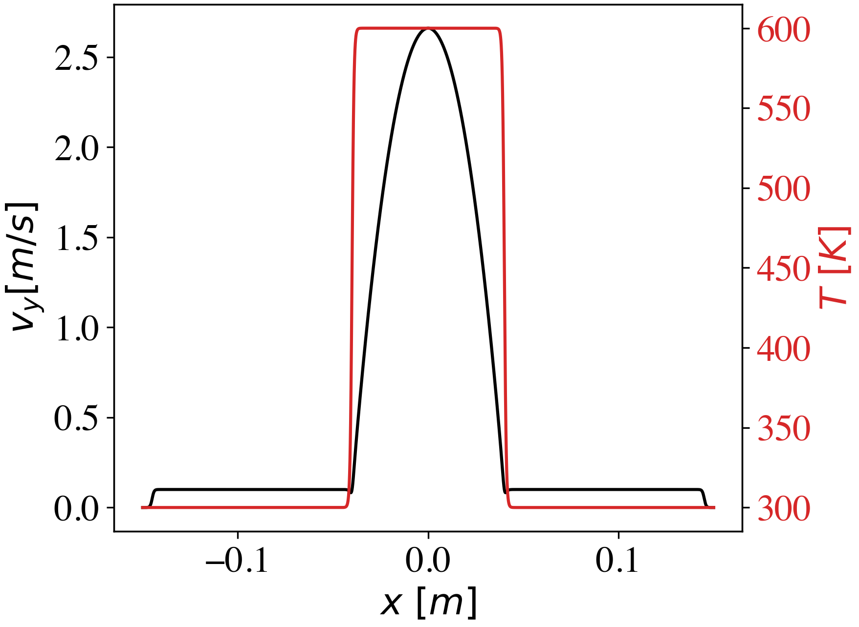
Figure 2: An example for the y-component of velocity, $v_{y}(x,0)$, and temperature profile, $T(x,0)$, of the heated fluid column at the bottom boundary of the simulated space. The following parameters were used: $c_{1}=1600\ m^{-1}\cdot s^{-1},\ c_{2}=0.1\ m\cdot s^{-1},\ c_{3}=2000\ m^{-1},\ d=0.08\ m,\ T_{0}=300\,K,\ H=0.3\ m$

In the equation from above, $d$ denotes the nozzle diameter, $H$ denotes the width of the simulated space, the parameters $c_{1},c_{2}$ determine the incoming flow rate of the fluid, and $c_{3}$ is a tuning parameter governing the cut in each profile.

At the upper boundary (height $L$), free boundary conditions are applied for the $y$ component of the velocity and for the $x$ component Dirichlet condition is applied, i.e. $v_{x}(x,L)=0$. For pressure, Dirichlet boundary conditions were used in the upper part of the simulated volume, $p(x,L)=g\cdot\rho_{0}\cdot l$, and free boundary condition for the other boundaries. The temperature on the walls is fixed to $T_{0}$. On the upper boundary we consider $T_{0}$ if the $y$-direction component of the velocity is negative, otherwise free boundary conditions are used. The temperature at the lower boundary is determined by using the equation:

$$T(x,0)=T_{0}+T_{heating}f\left(x,\frac{d}{2}\right)$$ (17)

Here, the $T_{heating}$ temperature governs the extra heat amount introduced in the system. For simplicity reasons we have used in all the presented results $T_{heating}=T_{0}$. In the first attempts at the upper part of the simulated box, free boundary condition were considered for the velocity. However in such cases unexpected instabilities occurred and after a certain time the heated fluid column was pushed on one of the sidewalls. We have examined carefully this phenomenon and concluded that a self-amplifying effect is responsible for its development. Due to the convective flow, the amount of fluid leaving the simulation box is larger than the volume of fluid flowing into the simulation box through the lower boundary. Since the fluid is incompressible, fluid must flow back into the simulation box through the upper boundary. Since there is always an asymmetry in the profile of the fluid inflow this will slightly deflect the outflowing column. In the direction of the deflection, the inflow area decreases, so the asymmetry in the fluid inflow increases. An increase in asymmetry over time will result in the fluid flowing along one of the walls. This is the simple explanation of the observed instabilty.

Two methods were used to eliminate these instabilities. The first method is to flow a fluid of ambient temperature $T_{0}$ at a constant rate on both sides of the heated air column. Since the flow is two-dimensional, the fluid flowing on a given side can only leave on the same side and this will always provide a minimum distance from the wall for the rising jet. The second method is to allow only the $y$-direction component of the velocity at the upper boundary. Combining this two methods will eliminate the tendency of the jet to approach one of the sidewalls.

For the upper boundary a proper boundary condition has to be applied also for the inflowing fluid temperature. At the upper boundary an inflow is also necessary in order to respect the incompressibility of the fluid. Since the temperature of the outflowing fluid varies over a wide range we can’t apply Dirichlet boundary condition to the whole upper boundary because this would cause unmanageable gradients. Avoiding large gradients due to large temperature differences was solved by applying boundary condition only to those points where the $y$-direction component of the velocity became negative.

The time series for the relevant hydrodynamical parameters were generated and we followed the temperature distribution in the simulated space. For realistically chosen parameters, it was shown that the model is capable to produce an oscillation similar to the one observed in the case of the Helium column. Interestingly, it was found that such oscillations are possible even on largely different length-scales. The observed oscillation is shown in Figure 3 a, b. where we illustrate the temperature space at subsequent time moments. For the simulations presented in Figure 3, we used the parameters spcified in the figure caption.

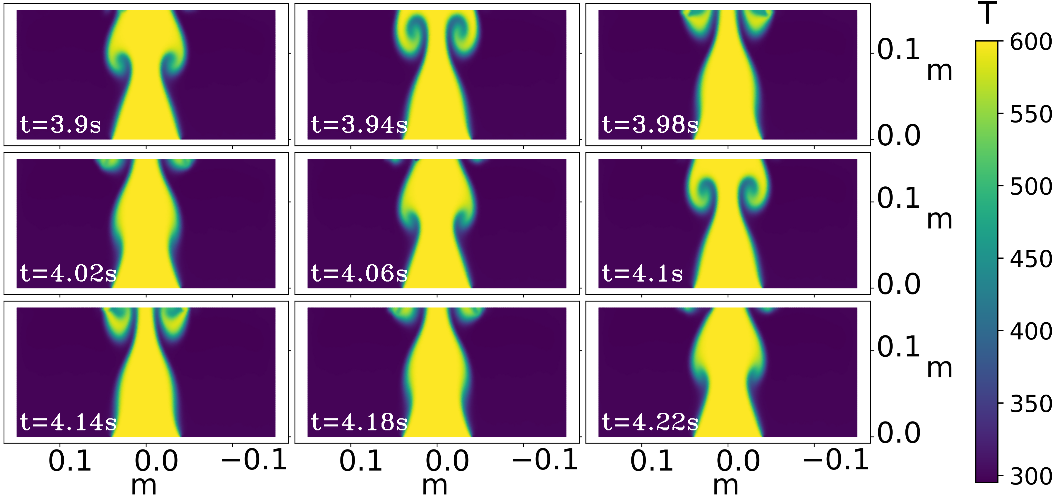
(a)

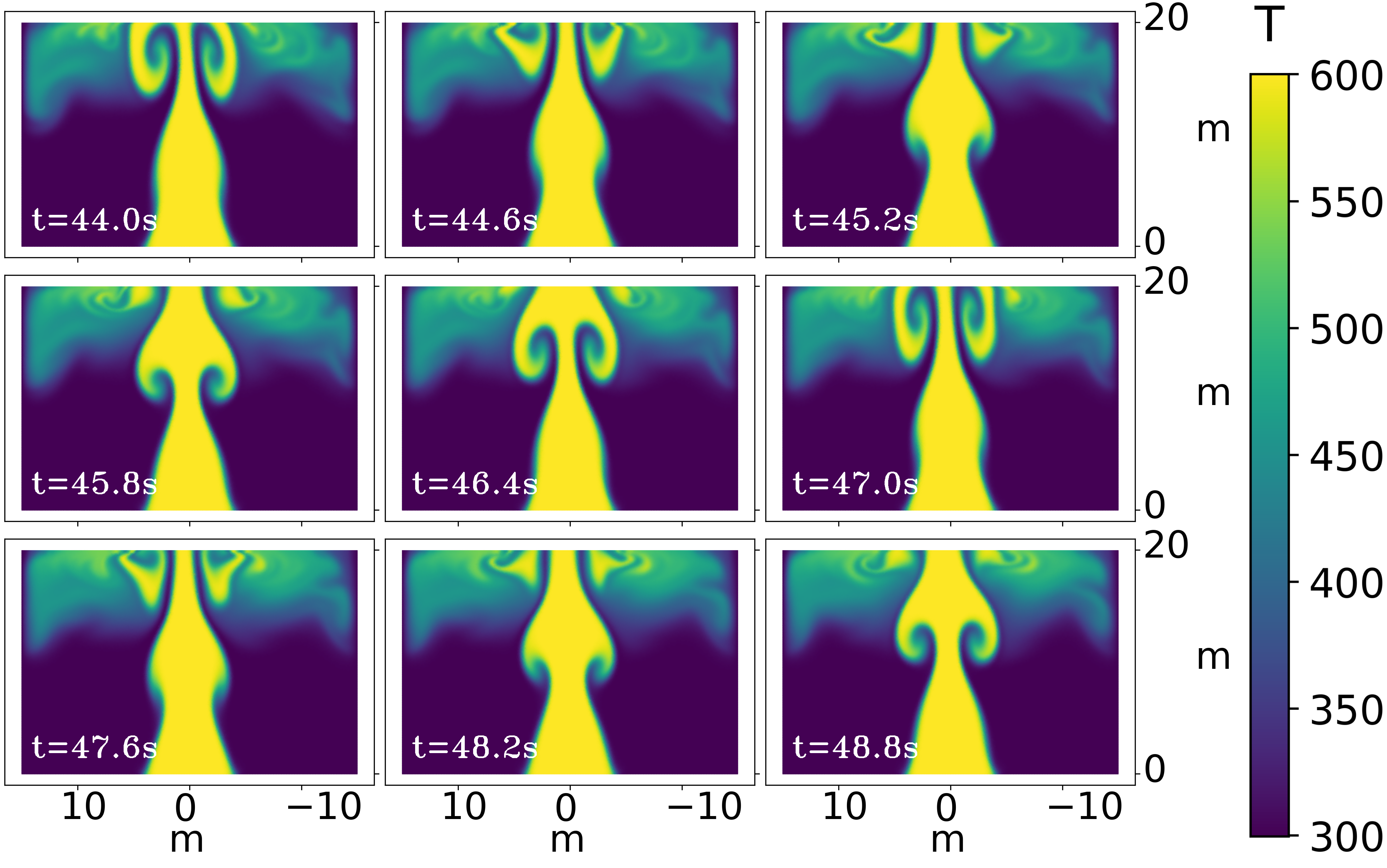
(b)

Figure 3: Oscillation of a heated air column in snapshots. The images show the temperature space at the specified $t$ time moments for two different length scales (Figures a. and b.). The gravity acts in the negative direction of the $y$-axis and the parameters of the simulation were chosen as follows: (a)$\ \alpha=0.33\cdot 10^{-2}\ K^{-1},\,\rho_{0}=1.2\ Kg\cdot m^{-2},\,T_{0}=300\ K,\,D=10^{-4}\ m^{2}\cdot s^{-1}\cdot K^{-1},\,g_{y}=-9.81\ m\cdot s^{-2},\,\mu=1.96\cdot 10^{-5}\ Kg\cdot s^{-1},\,c_{2}=0.1\ m\cdot s^{-1},\,c_{3}=2000\ m^{-1},\,d=0.08\ m,\,c_{1}=1600\ m^{-1}\cdot s^{-1}$,
(b) $\alpha=10^{-3}\ K^{-1},\,\rho_{0}=1\ Kg\cdot m^{-2},\,T_{0}=300\ K,\,D=5\cdot 10^{-2}\ m^{2}\cdot s^{-1}\cdot K^{-1},\,g_{y}=-9.81\ m\cdot s^{-2},\,\mu=5\cdot 10^{-2}\ Kg\cdot s^{-1},\,c_{2}=0.4\ m\cdot s^{-1},\,c_{3}=5\ m^{-1},\,d=8\ m,\,c_{1}=0.375\ m^{-1}\cdot s^{-1}$

For a quantitative evaluation of the simulated dynamics, the Otsu method was applied for the 2D temperature field. To obtain the time series, in uniform time intervals the Otsu processed pixels were summed up to a certain height, after this the obtained time series was divided by the average value of the time series. The oscillation frequency was calculated in a similar manner with the experiments, based on the above generated time series. In the first step a Fourier transform was applied to the time series and then the value of the frequency belonging to the largest peak was determined as the relevant oscillation frequency.

With the implemented simulation code we examined how the inflow rate (yield) of the heated fluid column and the nozzle diameter affects its oscillation frequency. We also investigated the collective behavior for the oscillation of two columns placed nearby each other.

II.3 Numerical results for the oscillation frequency

The effect of flow yield and nozzle diameter was examined on two different length-scales. To study the flow yield we used the parameter sets (a), (b) introduced above and the nozzle diameters were $d=0.08\ m$ and $d=8\ m$ respectively. For constant $c_{3}$, $c_{2}$, and $d$ parameters the yield (flow debit) of the heated fluid depends only on $c_{1}$:

$$\Phi=\int_{-\frac{d}{2}}^{\frac{d}{2}}v_{y}(x,0)\ dx=$$ (18)

$$=\int_{-\frac{d}{2}}^{\frac{d}{2}}[c_{1}f\left(x,\frac{d}{2}\right)\left(\frac{d}{2}-x\right)\left(x+\frac{d}{2}\right)+c_{2}f\left(x,\frac{H}{2}(1-\frac{1}{30})\right)]dx$$

The computed oscillation frequency of the heated fluid column as a function of the $\Phi$ parameter is plotted in Figure 5a and Figure 4a. One will observe that the oscillation frequency increases as the flow rate $\Phi$ increases and this increasing trend can be well approximated by a linear fit in good agreement with the experimental results plotted in Figure 6.

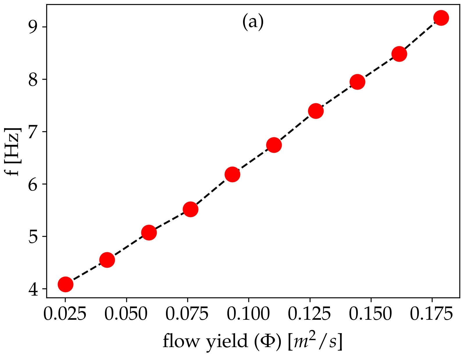
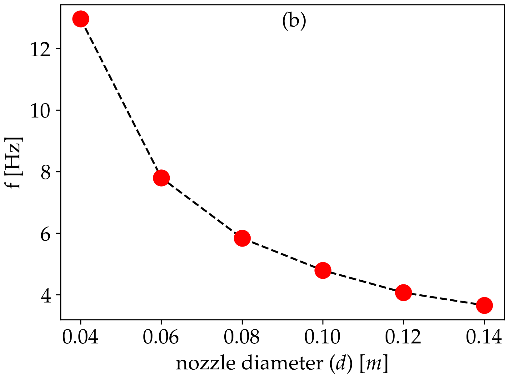
Figure 4: Simulation results for the smaller length-scale. Figure (a) shows the oscillation frequency of the heated fluid column as a function of the flow yield $\Phi$ fixed by equation (18) for $d\ =\ 0.08\ m$ inflow diameter. Figure (b) shows the oscillation frequency of the heated fluid column as a function of the $d$ nozzle diameter. The other parameters used are the same as the ones specified in the caption of Figure 3, the value of $c_{1}$ for the different nozzle diameters are given in Table 1.

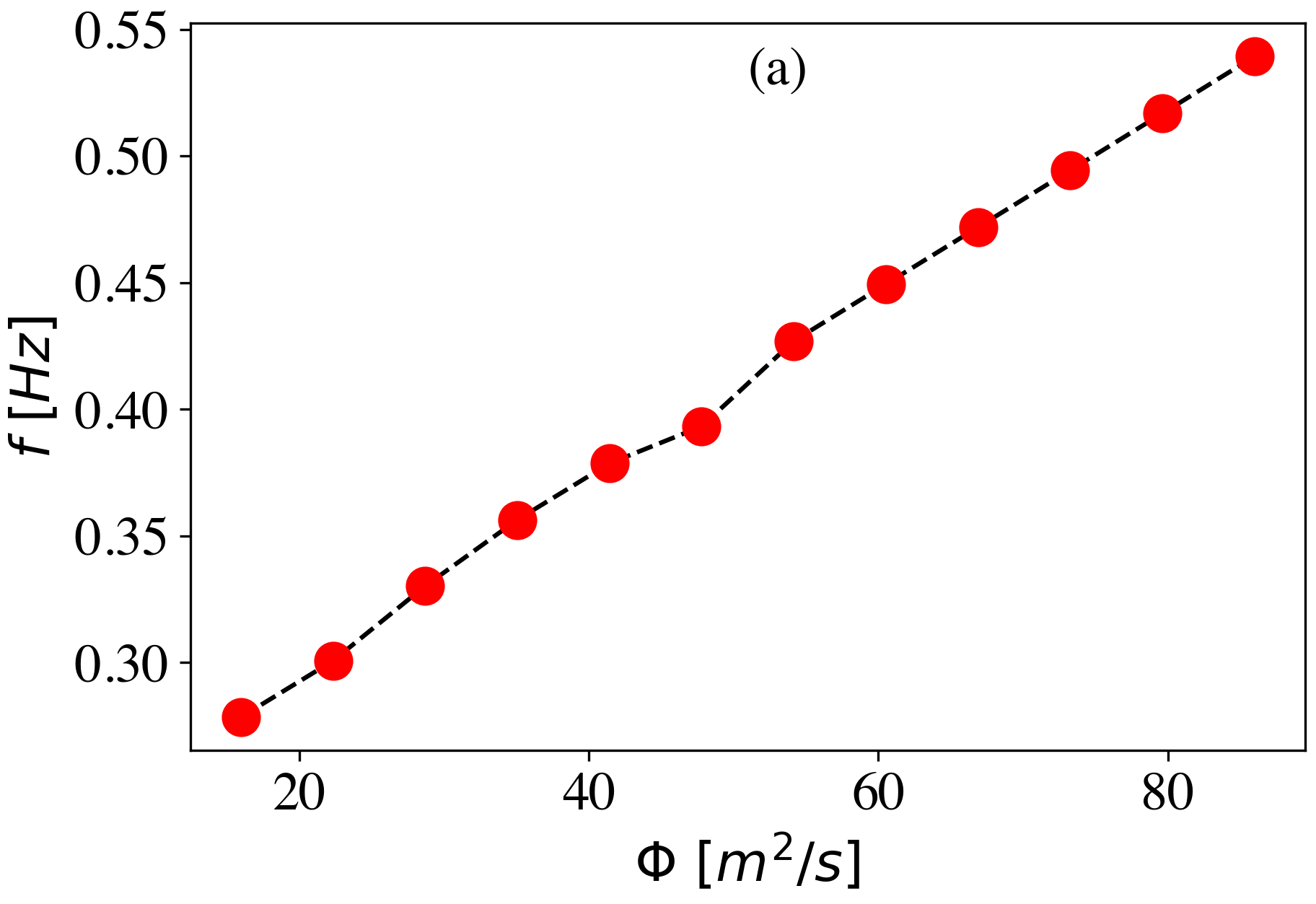
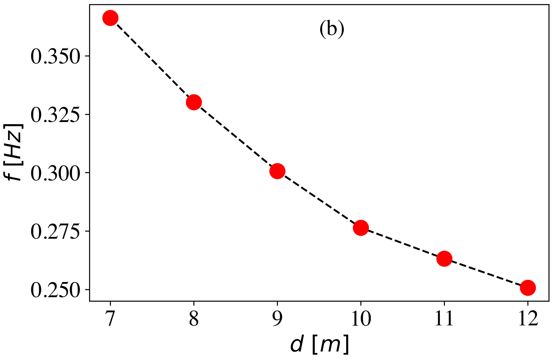
Figure 5: Simulation results for the larger length-scale. Figure (a) shows the oscillation frequency of the heated fluid column as a function of the flow yield $\Phi$ fixed by equation (18) for $d\ =8\ m$ inflow diameter. Figure (b) shows the oscillation frequency of the heated fluid column as a function of the $d$ nozzle diameter. The other parameters are the same as the ones specified in the caption of Figure 3, the value of $c_{1}$ for the different nozzle diameters are given in Table 2.

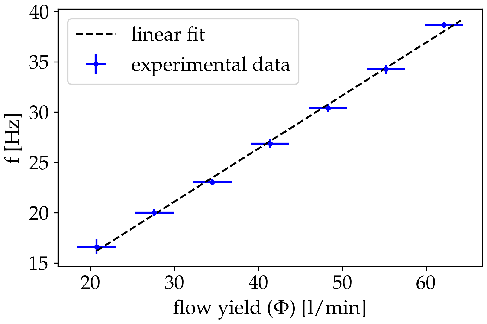
Figure 6: Experimentally observed oscillation frequency of a Helium column as a function of the yield (flow debit) obtained for a setup with nozzle diameter of 2 cm. With increasing flow yield, the frequency of the oscillation increases in an almost linear manner. The plot is done by using the results presented in Gergely et al. (2021). Error bars show the uncertainty in the measurement of the flow yield.

The effect of nozzle diameter on the oscillation frequency was investigated at a constant inflow yield. Since the yield $\Phi$ depends on $d$ according to equation (18), for different nozzle diameters we must rescale the parameters $c_{1}$ so that the flow rate remains constant. For the smaller length-scale simulations, we used $\Phi_{1}=0.076\ m^{2}/s$ flow yield and for the larger scale simulations, we used $\Phi_{2}=29\ m^{2}/s$ flow yield. To keep constant the flow yield for different nozzle diameters, we varied the value of the $c_{1}$ parameter. The $c_{1}$ values for the different nozzle diameters are shown in Table 1 and Table 2.

d [m]	0.04	0.06	0.08	0.1	0.12	0.14
$c_{1}\ [m^{-1}\cdot s^{-1}]$	6781	1952	800	398	223	136

Table 1: Value of the $c_{1}$ parameter for different nozzle diameters $d$, in order to keep the flow rate $\Phi_{1}=0.076\ m^{2}/s$.

d [m]	7	8	9	10	11	12
$c_{1}\ [m^{-1}\cdot s^{-1}]$	0.45	0.3	0.21	0.153	0.11	0.088

Table 2: Value of the $c_{1}$ parameter for different nozzle diameters $d$, in order to keep the flow rate $\Phi=29\ m^{2}/s$.

For both length scales a decreasing trend of the oscillation frequency as a function of the nozzle diameter was observed. Results in such sense are plotted in Figure 5b and Figure 4b, the trend is in good agreement with the experimental results from Figure 7.

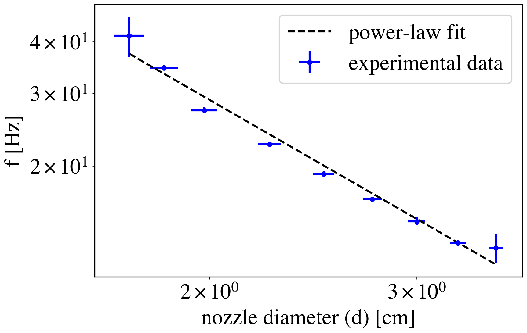
Figure 7: Experimentally observed oscillation frequency of a Helium column as a function of the nozzle diameter for a yield of $\Phi=$46 $\pm$ 2.3 $l/min$. The plot is done by using the results presented in Gergely et al. (2021). Error bars show the variations of the experimentally used nozzle diameter in different directions.

II.4 Numerical results for the collective behavior

We turn now our interest on reproducing the experimentally observed collective behaviour in form of anti-phase synchronization.

The dimensions of the simulation boxes used to study the collective behavior are the following: 46 m wide (H=46 m) and 30 m high (L=30 m) for the large length-scale and 0.3 m wide (H=0.3 m) and 0.15 m high (L=0.15 m) at the smaller length-scale. At the lower boundary, the $x$ component of the inflow fluid velocity is 0, and the $y$ component is given by the following kernel function:

$$v_{y}(x,0)=c_{1}f\left(x-d_{0},\frac{d}{2}\right)\left(d_{0}-x+\frac{d}{2}\right)\left(x-d_{0}+\frac{d}{2}\right)+$$

$$+c_{1}f\left(x+d_{0},\frac{d}{2}\right)\left(\frac{d}{2}-d_{0}-x\right)\left(x+d_{0}+\frac{d}{2}\right)+c_{2}f\left(x,\frac{H}{2}-c_{4}\right)$$

Here the value of $c_{4}$ is $0.5\ m$ for the large scale system and $0.005\ m$ for the small scale system.

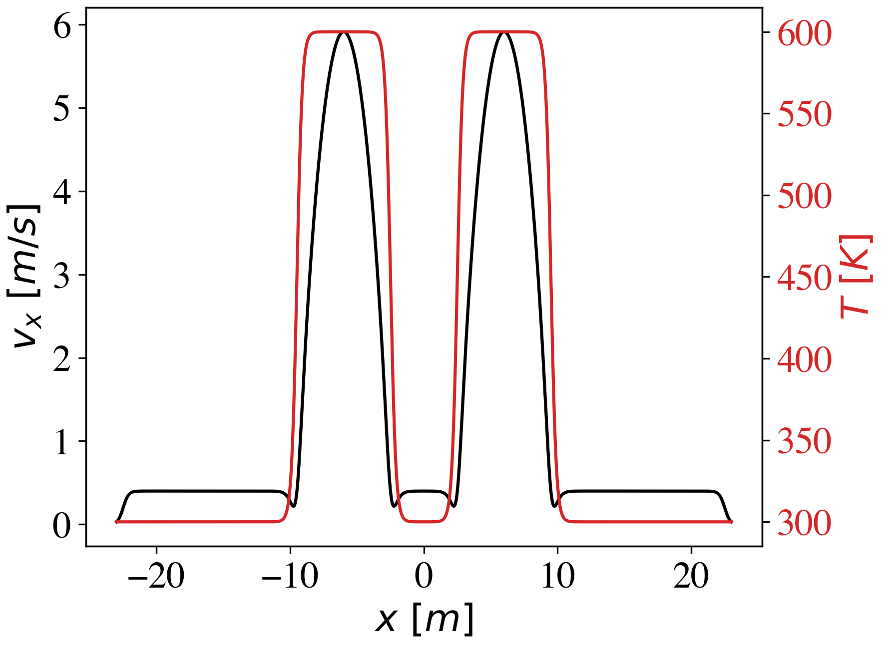
Figure 8: An example for the y-component velocity, $v_{y}(x,0)$, and temperature, $T(x,0)$, profiles of the heated fluid columns at the bottom boundary of the simulated space. The following parameters were used:$c_{1}=0.45\ m^{-1}\cdot s^{-1},\ c_{2}=0.4\ m\cdot s^{-1},\ c_{3}=5\ m^{-1},\ d=7\ m,\ d_{0}=6\ m,\ T_{0}=300\ K,\ H=46\ m$.

This leads to an inflow profile with two peaks where the centers are separated at a distance of $2d_{0}$, as it is illustrated in Figure 8. The temperature profile is adjusted accordingly:

$$T(x,0)=T_{0}+T_{heating}f\left(x-d_{0},\frac{d}{2}\right)+T_{heating}f\left(x+d_{0},\frac{d}{2}\right)$$

We used the same simulation parameters as before and fixed $d=7\ m$, $c_{1}=0.45\ m^{-1}\cdot s^{-1}$ values for the large length-scale and $d=0.04\ m$, $c_{1}=6400\ m^{-1}\cdot s^{-1}$ values for the small length-scale system. Again, for the presented results we considered $T_{heating}=T_{0}$. Experimental results from Gergely et al. (2021) shows that at small separation distance collective behavior in form of counter-phase synchronization appears. A snapshot for a simulated stable collective behavior is visible in Figure 9, reproducing successfully this counter phase synchronization on the smaller length-scale. Similar behavior is observable for the larger length-scales as well.

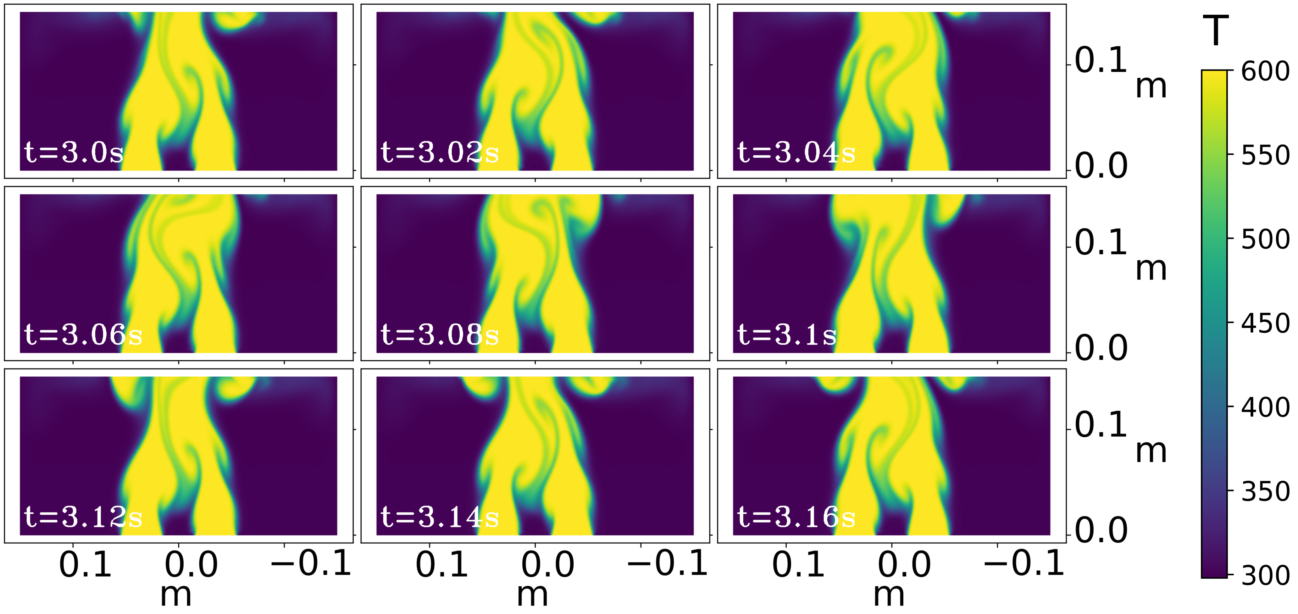
Figure 9: Counter-phase synchronization of two nearby heated columns. Computer simulation results with the following parameters: $\ \alpha=0.33\cdot 10^{-2}\ K^{-1},\,\rho_{0}=1.2\ Kg\cdot m^{-2},\,T_{0}=300\ K,\,D=10^{-4}\ m^{2}\cdot s^{-1}\cdot K^{-1},\,g_{y}=-9.81\ m\cdot s^{-2},\,\mu=1.96\cdot 10^{-5}\ Kg\cdot s^{-1},\,c_{2}=0.1\ m\cdot s^{-1},\,c_{3}=2000\ m^{-1},\,d=0.04\ m,\,c_{1}=6400\ m^{-1}\cdot s^{-1},\ H=0.3\ m$

For the pictures processed with the Otsu method the collective oscillation of nearby heated fluid columns are shown in Figures 10 a and b, for the small and large length-scales, respectively.

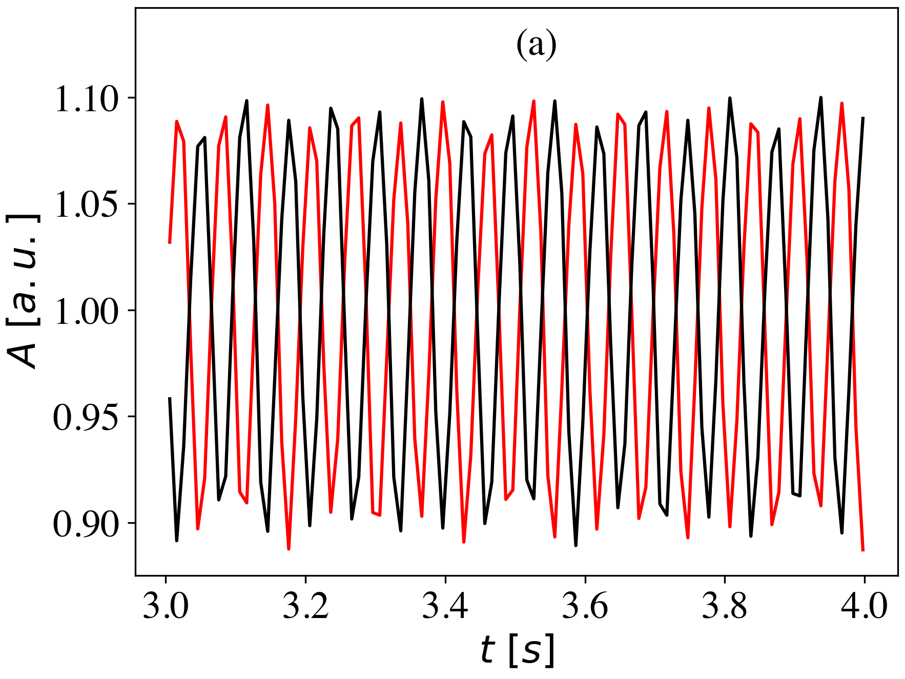
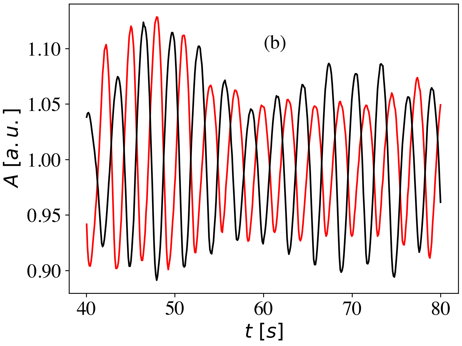
Figure 10: Simulated time series for the oscillations of nearby heated fluid columns. Motion of the interface is detected by the Otsu method at the same height from the nozzle. For not too high separation distances ((a) $2\cdot d_{0}=0.03\ m$ , (b) $2\cdot d_{0}=5\ m$) a clear counter-phase synchronization is observable. The parameters of the simulations are
(a): $\ \alpha=0.33\cdot 10^{-2}\ K^{-1}$, $\rho_{0}=1.2\ Kg\cdot m^{-2}$, $T_{0}=300\ K$, $D=10^{-4}\ m^{2}\cdot s^{-1}\cdot K^{-1}$,  $g_{y}=-9.81\ m\cdot s^{-2}$, $\mu=1.96\cdot 10^{-5}\ Kg\cdot s^{-1}$, $c_{2}=0.1\ m\cdot s^{-1}$, $c_{3}=2000\ m^{-1}$, $d=0.04\ m$, $c_{1}=6400\ m^{-1}\cdot s^{-1}$, $2\cdot d_{0}=0.03\ m$.
(b): $\alpha=10^{-3}\ K^{-1}$, $\rho_{0}=1\ Kg\cdot m^{-2}$, $T_{0}=300\ K$, $D=5\cdot 10^{-2}\ m^{2}\cdot s^{-1}\cdot K^{-1}$, $g_{y}=-9.81\ m\cdot s^{-2}$, $\mu=5\cdot 10^{-2}\ Kg\cdot s^{-1}$, $c_{2}=0.4\ m\cdot s^{-1}$, $c_{3}=5\ m^{-1}$, $d=8\ m$, $c_{1}=0.375\ m^{-1}\cdot s^{-1}$, $2\cdot d_{0}=0.03\ m$ and we have fixed $d=7$ and $c_{1}=0.45\ m^{-1}\cdot s^{-1}$.

For the indicated smaller separation distances an almost perfect counter-phase synchronization develops. For larger separation distances the phases of the oscillations will begin to shift relative to each other and no clear phase-difference blocking is observable.

For the simulations performed on the smaller length-scale, corresponding to the experimental conditions in Gergely et al. (2021) we computed the synchronization order parameter which is meant to characterize the collective oscillation. We used the same $z$ synchronization order parameter as the one used in Gergely et al. (2020) and Gergely et al. (2021). The computationally derived synchronization parameter is plotted in Figure 11 a. It’s values in the neighborhood of -1 indicates that we have counter-phase synchronization for the studied distances. In Figure 11b we also show the oscillation frequency of the two synchronized heated fluid columns as a function of their separation distance. This frequency decreases as we increase the separation distance between the columns, similarly with what has been reported in our experiments for the Helium columns Gergely et al. (2021).

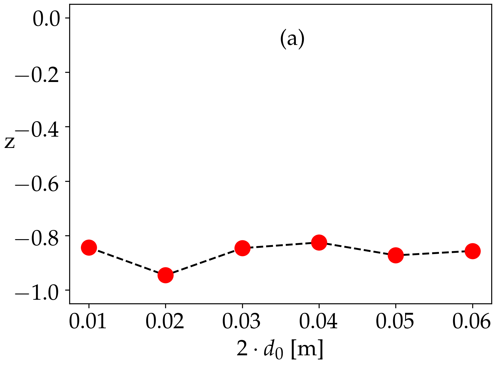
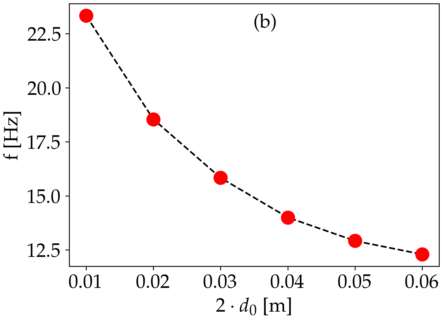
Figure 11: Simulation results for the collective behavior of two heated columns. Figure (a) the synchronization order parameter of two interacting heated fluid columns and Figure (b) shows the collective oscillation frequency, both as a function of the separation distance between the columns. The following simulation parameters were considered: $\ \alpha=0.33\cdot 10^{-2}\ K^{-1},\,\rho_{0}=1.2\ Kg\cdot m^{-2},\,T_{0}=300\ K,\,D=10^{-4}\ m^{2}\cdot s^{-1}\cdot K^{-1},\,g_{y}=-9.81\ m\cdot s^{-2},\,\mu=1.96\cdot 10^{-5}\ Kg\cdot s^{-1},\,c_{2}=0.1\ m\cdot s^{-1},\,c_{3}=2000\ m^{-1},\,d=0.04\ m,\,c_{1}=6400\ m^{-1}\cdot s^{-1}$

III Discussion and Conclusions

In our previous study Gergely et al. (2021), we used both experimental and theoretical approaches to investigate whether the hydrodynamic instabilities that occur in rising gas columns is responsible also for the oscillations observed for the diffusion flames Gergely et al. (2020). It was shown that indeed this is the case: Helium columns ascending in air from a circular nozzle produce similar oscillations with the ones observed in diffusion flames. Also, the similar collective behavior of these oscillations (counter-phase synchronization) for Helium columns and flickering candle flames suggest that the hydrodynamic processes by their own are enough to explain these phenomenon.

In our previous work Gergely et al. (2021), for modeling the observed oscillations , a simplified but analytically treatable hydrodynamical approach was used. The model predicted the right trends for the oscillation frequencies as a function of the relevant parameters, but was unsuitable to approach the collective behavior. In the present follow-up, we offered an improved modeling by considering a 2D numerical hydrodynamics computer simulation where for computational simplicity instead of ascending Helium columns, heated fluid columns were considered. This approach proved to be successful for reproducing all the experimentally observed features. For a constant nozzle diameter the numerical hydrodynamics approach lead to an oscillation frequency that increased roughly linearly with the flow yield, in agreement with the experimental results. For constant flow yield the numerical results suggested a decreasing trend of the oscillation frequency as a function of the nozzle diameter, confirming the experimental results. The exact shape of the simulated trend was slightly different however from the one observed in the experiments. The main reason for this discrepancy is probably the reduction of the real 3D problem to a 2D topology. Finally, the presented computer simulations were successful also in reproducing the counter-phase synchronization of two heated fluid columns placed nearby each other. The computed trends for the synchronization order-parameter and the collective frequency were also in agreement with the experimental results obtained for rising Helium columns in air.

It worth mentioning here that the computer simulations were performed both for laboratory and for a much larger length-scale than the experiments. The qualitative agreement between the results (trends and collective behavior) on these different length-scales suggests that the investigated phenomenon is more general than it was thought to be, and might have further, yet unexplored connections.

Acknowledgment We acknowledge Dr. M. Ercsey-Ravasz, Dr. B. Molnár, and Prof. dr. G.C. Silaghi, all from the Babes-Bolyai University in helping us with the computational resources for running our simulation codes.

Appendix

A. Solving the 2D Poison equation in FEniCS

Here we illsutrate through the 2D Poison equation how to solve a PDE in FEniCS. The Poisson equation can be given in the following form:

$$-\Delta\varphi=f$$ (21)

If we have a simple rectangular space then the above equation can be easily given in the finite element form

$$-\frac{\varphi_{i-1,j}-2\varphi_{i,j}+\varphi_{i+1,j}}{h^{2}}-\frac{\varphi_{i,j-1}-2\varphi_{i,j}+\varphi_{i,j+1}}{h^{2}}=f_{i,j},$$ (22)

however, with this simple and intuitive approach, we soon run into problems because even for a circle it is impossible to map the boundary with an acceptably small number of squares. The FEniCS program Langtangen and Logg (2017) uses a triangular grid instead of a square grid to cover the simulated space, in which case we can always select the grid so that the grid points are on the boundary surfaces. Discretization alone does not solve the equation, the next question is how to determine the solution at each lattice point. As a first step, we write the $\varphi(x_{1},x_{2})$ function in the following form:

$$\varphi(x_{1},x_{2})=\sum_{i=0}^{N}c_{i}\phi_{i}(x_{1},x_{2})$$ (23)

In the above equation, $\phi_{i}(x_{1},x_{2})$ is a given k-th order polynomial, $c_{i}$ are the coefficients that determine $\varphi(x_{1},x_{2})$ and N+1 is the number of the grid points. The $c_{i}$ coefficients are determined by multiplying the Poison equation by N+1 different $v(x_{1},x_{2})$ so-called test functions and integrating the product over the whole domain to obtain N + 1 linearly independent equations from which the $c_{i}$ coefficients can be calculated. All this can be formally given in the following form:

$$\int_{\Omega}-v\,\Delta\varphi\ d\Omega=\int_{\Omega}fv\ d\Omega$$ (24)

We denoted by $d\Omega=dx_{1}dx_{2}$.The above form of PDE is called the weak formulation of the equation and this is what is calculated by the FEniCS program. The second-order coordinate derivative in the above equation means that the polynomials used need to be twice differentiable. Because the use of polynomials with large degrees requires more memory and computation, we always strive to keep the degree of polynomials to a minimum. In the above equation, the reduction of the order of derivatives can be done by Gauss-Green integration as follows:

$$\int_{\Omega}-v\,\Delta\varphi\ d\Omega=\int_{\Omega}\nabla v\nabla\varphi\ d\Omega-\int_{\partial\Omega}\frac{\partial\varphi}{\partial{\bf n}}v\ d{s}$$ (25)

Since we use Dirichlet boundary conditions for the Poisson problem, the value of $v$ at the boundary is 0, so the equation (24) can be written in the following form:

$$\int_{\Omega}\nabla v\nabla\varphi\ d\Omega=\int_{\Omega}f\,v\ d\Omega$$ (26)

We have seen above how to rewrite the 2D Poisson problem in a form that can be solved with the FEniCS program, now we show the implementation of the solution in Python.

⬇

from fenics import * #

import numpy as np #Numpy is required for error calculation

import matplotlib.pyplot as plt #We plot the result with the matplotlib

Nx=10#The number of grid points in the x directions

Ny=10#The number of grid points in the y directions

mesh=UnitSquareMesh(Nx,Ny)

V=FunctionSpace(mesh,’P’,1)#space containing first degree polynomials

fi_D=Expression(’1+x[0]*x[0]+2*x[1]*x[1]’,degree=2)

#boundary conditions equation (on boundarys fi(x,y)=x^2+2y^2+1)

def boundery(x,on_boundary):

return on_boundary

bc=DirichletBC(V,fi_D,boundery)#boundary conditions

fi=TrialFunction(V)

v=TestFunction(V)

f=Constant(-6)

a=dot(grad(fi),grad(v))*dx#right side of equation

L=f*v*dx#left side of equation

fi=Function(V)

solve(a==L,u,bc)#solve the equation

c = plot(interpolate(fi, V), mode=’color’)

plt.colorbar(c)

plot(fi)

plt.savefig(’result1.png’)

plt.show()

vertex_v_ud=fi_D.compute_vertex_values(mesh)

vertex_v_u=fi.compute_vertex_values(mesh)

err_max=np.max(np.abs(vertex_v_ud-vertex_v_u))

print("maximum␣error:␣",err_max)

The above program solves equation (21) on the unit square of $\{(0,0),(1,1)\}$. The largest difference between the theoretically expected and the numerically obtained value was of the order of the precision of the numerical representation of the numbers, giving us confidence for the use of the numerical solution.

B. Test for the 2D hydrodynamics simulations. Karman vortices

The first phenomenon we aimed to reproduce using our fluid dynamics simulation is the formation of Karman vortices in the flow of fluids around an obstacle. With this test we aimed to check visually whether the Navier-Stokes equation has been correctly implanted, since the temperature of the fluid at all points is considered fixed: $T_{0}$. Therefore for this test the density in the simulated volume is constant.

In these simulations, the length of the simulated volume was considered as $2.2$m, the width of the simulated volume is $0.41$m and in the middle of the simulated coordinate space a circular obstacle with a radius of $0.05$m is placed. The coordinates of the centre of this obstacle was taken at (0.2m, 0.2m). The density of the fluid was taken as unity (1kg/m²), the viscosity is $0.001$kg/s, and no gravitational field is considered. For input (the left region of the space in Figure 12) we considered that the velocity in the $y$ direction is $0$, the velocity in the $x$ direction has a parabolic profile with a maximum value of $1.5$m/s. On the horizontal walls and on the boundary of the obstacle we consider no-slip conditions, thus the velocity is fixed to $0$. For the output (right-sight region) we have also imposed for the $y$ direction velocity to be zero, and the pressure at the output is fixed also to $0$. Elsewhere there are all free boundary conditions for the pressure. The temperature is fixed at $T_{0}=300$K at input and on the horizontal walls.

The velocity vector spaces obtained from the simulations are shown in Figure 12 for $4$ time moments as it is indicated on the left side of the images. One can observe that the simulation reproduces successfully the expected Karman vortices.

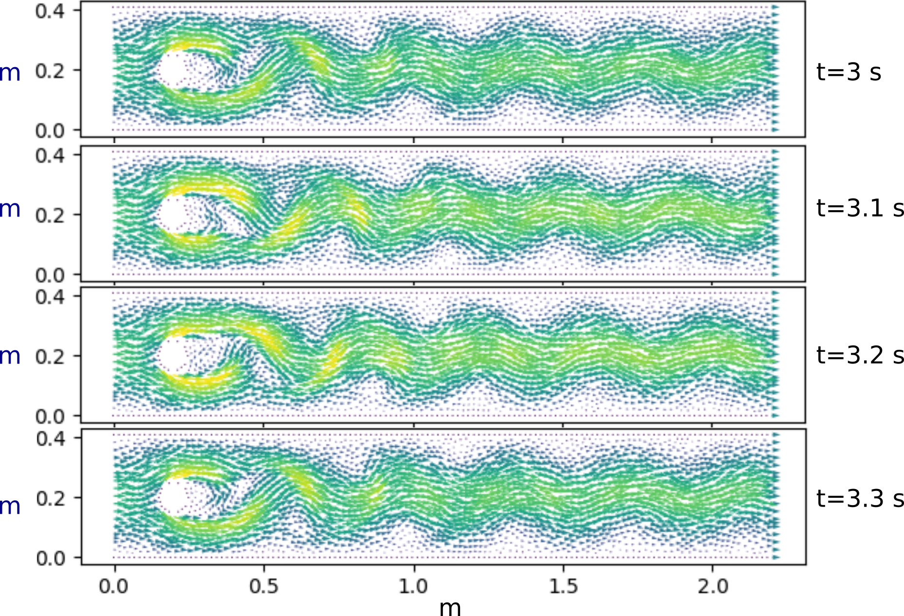
Figure 12: Velocity fields obtained from the simulation of the Karman vortices at four consecutive time moments.

C. Test for the 2D hydrodynamics simulations. Heat induced mushroom cloud

In this second test we aimed to implement the density and temperature evolution of a heated gas sphere in gravitational field. It is expected that the shape of the heated gas will follow the known dynamics of a mushroom cloud in a nuclear explosion.

In the performed simulations, the density at $T_{0}$ was chosen as unity ($1$kg/m²), the ambient temperature $T_{0}$ is $300$K, the $\alpha$ parameter in equation (2) is $\alpha=0.001\ K^{-1}$, the thermal diffusion constant $D$ is $0.3$m²/s, the initially heated sphere temperature is $600$K, the fluid viscosity is taken as $\mu=0.05$kg/s, the gravitational acceleration is $g_{y}=-9.81$m/s² and the size of the simulated volume is $30$m² in both the $x$ and $y$ directions.

At the bottom and walls of the simulated space, the velocity is fixed to $0$, at the upper boundary, we fix the $x$ component of the velocity to $v_{x}=0$. For the pressure, the value of $g\cdot\rho_{0}\cdot l$ is fixed for the upper boundary, and free boundary conditions are applied to all the other boundaries. For temperature, free boundary condition is applied at the upper boundary if the $y$ direction component of the velocity is positive otherwise the temperature is fixed to $T_{0}=300$K units on the upper boundary and on the side-walls. The temperature is fixed to a higher value of $450$K units at the bottom-wall of the simulated area. This is necessary in order to make the resulting flow visible in the temperature space. Initially, the velocity in the whole simulated volume is $0$ and the volume contains a sphere (disk) with a radius of $5$m in which the temperature is $600$K. The centre of the sphere is at the coordinates (0m, 7m), the temperature around the sphere is fixed to $300$K, and the temperature between the centre and the surface of the disk is given by an interpolation with a sigmoid function.

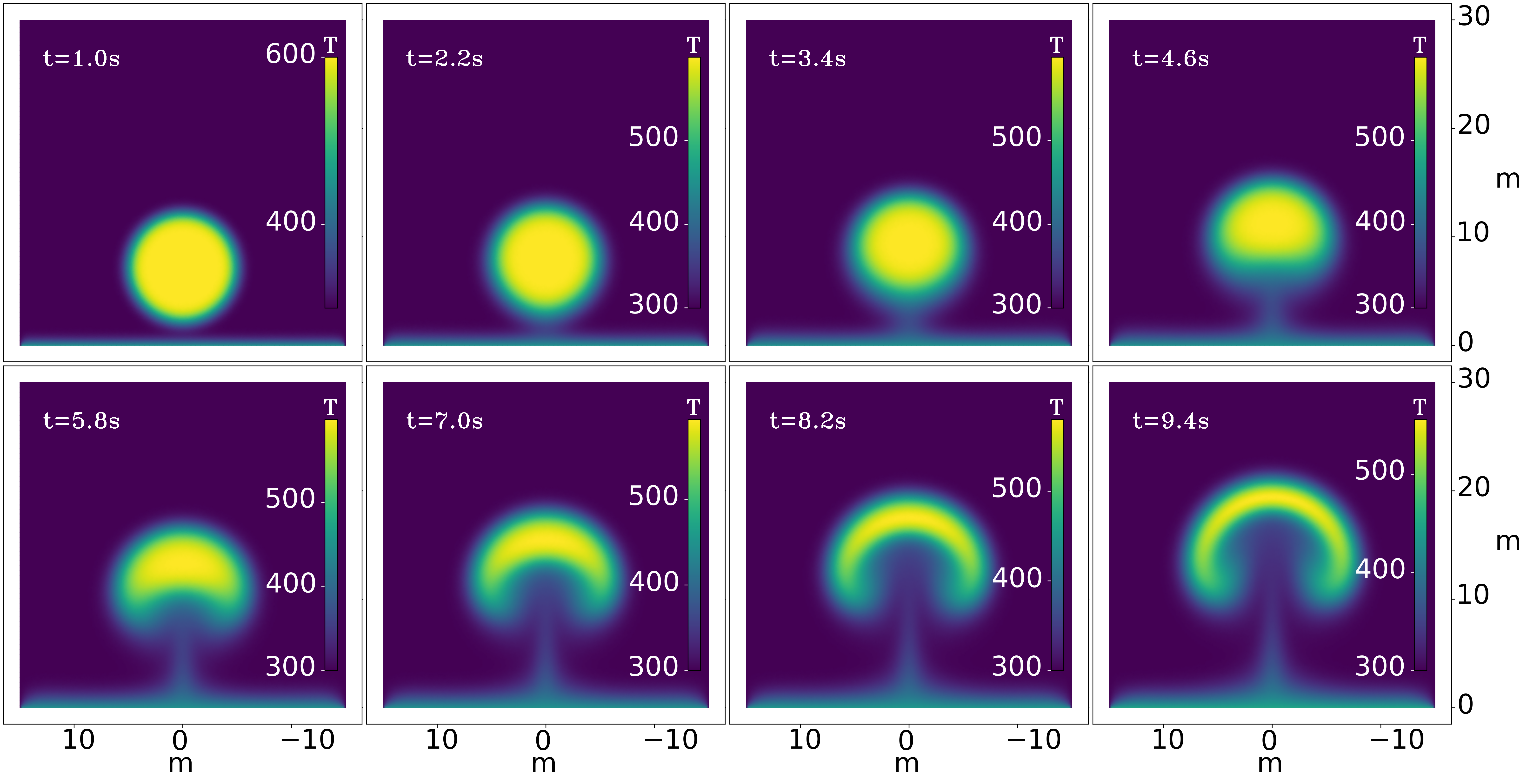
Figure 13: Snapshots of the evolution of a heated gas sphere in time. The parameters and details of the simulation can be found in the text.

The time-evolution of the temperature map derived from the simulation is shown in Figure 13. The effect of thermal diffusion can be observed in the first two frames. As a result of this diffusion the initially sharp boundary line between the high and low temperature regions gets blurred. Subsequent frames show the displacement due to convective flow and as a result of this the characteristic mushroom cloud shape is formed.

References

- Gergely et al. (2021) A. Gergely, C. Paizs, R. Tötös, and Z. Néda, “Oscillations and collective behavior in convective flows,” Physics of Fluids 33, 124104 (2021).
- Yuan, Durox, and Villermaux (1994) T. Yuan, D. Durox, and E. Villermaux, “An analogue study for flame flickering,” Experiments in Fluids 17, 337–349 (1994).
- Chamberlin and Rose (1948) D. Chamberlin and A. Rose, “The flicker of luminous flames,” Proceedings of the Symposium on Combustion 1-2, 27–32 (1948).
- Durox et al. (1995) D. Durox, T. Yuan, F. Baillot, and J. Most, “Premixed and diffusion flames in a centrifuge,” Combustion and Flame 102, 501–511 (1995).
- Durox, Yuan, and Villermaux (1997) D. Durox, T. Yuan, and E. Villermaux, “The effect of buoyancy on flickering in diffusion flames,” Combustion Science and Technology 124, 277–294 (1997).
- Huang et al. (1999) Y. Huang, Y. Yan, G. Lu, and A. Reed, “On-line flicker measurement of gaseous flames by image processing and spectral analysis,” Measurement Science and Technology 10, 726–733 (1999).
- Kitahata et al. (2009) H. Kitahata, J. Taguchi, M. Nagayama, T. Sakurai, Y. Ikura, A. Osa, Y. Sumino, M. Tanaka, E. Yokoyama, and H. Miike, “Oscillation and synchronization in the combustion of candles,” The Journal of Physical Chemistry A 113, 8164–8168 (2009).
- Ghosh et al. (2010) S. Ghosh, S. Mondal, T. Mondal, A. Mukhopadhyay, and S. Sen, “Dynamic characterization of candle flame,” International Journal of Spray and Combustion Dynamics 2, 267–284 (2010).
- Okamoto et al. (2016) K. Okamoto, A. Kijima, Y. Umeno, and H. Shima, “Synchronization in flickering of three-coupled candle flames,” Scientific Reports 6 (2016), 10.1038/srep36145.
- Chen et al. (2019) T. Chen, X. Guo, J. Jia, and J. Xiao, “Frequency and phase characteristics of candle flame oscillation,” Scientific Reports 9 (2019), 10.1038/s41598-018-36754-w.
- Gergely et al. (2020) A. Gergely, B. Sándor, C. Paizs, R. Tötös, and Z. Néda, “Flickering candle flames and their collective behavior,” Scientific Reports 10 (2020), 10.1038/s41598-020-78229-x.
- Settles (2001) G. S. Settles, Schlieren and Shadowgraph Techniques : Visualizing Phenomena in Transparent Media (Springer Berlin Heidelberg, Berlin, Heidelberg, 2001).
- Leptuch and Agrawal (2006) P. A. Leptuch and A. K. Agrawal, “High-speed rainbow schlieren visualization of an oscillating helium jet undergoing gravitational change,” Journal of Visualization 9, 101–109 (2006).
- Otsu (1979) N. Otsu, “A threshold selection method from gray-level histograms,” IEEE Transactions on Systems, Man, and Cybernetics 9, 62–66 (1979).
- FreddyCree (2020) FreddyCree, Wikipedia, Otsu’s method (2017 (accessed July 11, 2020)).
- Gergely (2020a) A. Gergely, (2020 (accessed November 10, 2020)a), https://youtube.com/playlist?list=PLamJmxTyiR_3sy-fYUEDEXW4NtbsnsXnW.
- Joel H. Ferziger and Street (2020) M. P. Joel H. Ferziger and R. L. Street, Computational Methods for Fluid Dynamics, 4th edition (Springer International Publishing, 2020).
- Wendt (2009) J. F. Wendt, Computational Fluid Dynamics (Springer Berlin Heidelberg 2009, 2009).
- V. Venkatakrishnan and R. Chakravarthy (1998) M. D. S. V. Venkatakrishnan and e. R. Chakravarthy, Barriers and Challenges in Computational Fluid Dynamics (Springer Science+Business Media Dordrecht, 1998).
- Correa et al. (2019) P. G. Correa, J. MacIntyre, J. Gomba, M. Cachile, J. Hulin, and A. Auradou, “Three-dimensional flow structures in x-shaped junctions: Effect of the reynolds number and crossing angle,” Physics of Fluids 31, 043606 (2019).
- Gergely (2020b) A. Gergely, Heated air column (2020 (accessed November 10, 2020)b), https://youtube.com/playlist?list=PLamJmxTyiR_0fNk5bzTD5GyRF_dOrmB2E.
- Langtangen and Logg (2017) H. P. Langtangen and A. Logg, Solving PDEs in Python (Springer, 2017).
- Logg et al. (2012) A. Logg, K.-A. Mardal, G. N. Wells, et al., Automated Solution of Differential Equations by the Finite Element Method (Springer, 2012).