Efficient evaluation of expectations of functions of a Lévy process and its extremum

Abstract.

We prove a simple general formula for the expectation of a function of a Lévy process and its running extremum. Under additional conditions, we derive analytical formulas using the Fourier/Laplace inversion and Wiener-Hopf factorization, and discuss efficient numerical methods for realization of these formulas. As applications, the cumulative probability distribution function of the process and its running supremum and the price of the option to exchange the supremum of a stock price for a power of the price are calculated. The most efficient numerical methods use the sinh-acceleration technique and simplified trapezoid rule. The program in Matlab running on a Mac with moderate characteristics achieves the precision E-7 and better in several milliseconds, and E-14 - in a fraction of a second.

Key words: Lévy process, extrema of a Lévy process, lookback options, barrier options, Wiener-Hopf factorization, Fourier transform, Laplace transform, Hilbert transform, Gaver-Wynn Rho algorithm, sinh-acceleration

MSC2020 codes: 60-08,42A38,42B10,44A10,65R10,65G51,91G20,91G60

1. Introduction

There exists a large body of literature devoted to calculation of the expectation of a function of a Lévy process and its running extremum, and related optimal stopping problems, standard examples being barrier and American options, and lookback options with barrier and/or American features. The general formulas for single barrier options with continuous monitoring were derived in [13, 14, 15] using the operator form of the Wiener-Hopf factorziation [40], under certain regularity conditions on the characteristic exponent. In [10], the same formulas were proved for any Lévy process. The first contribution of the paper is a similar simple general formula for the expectation of a function of a Lévy process and its running extremum, evaluated at a deterministic time $T>0$.

The pricing formulas are in terms of Laplace-Fourier inversion in dimensions 2 (first touch digitals and no-touch options), 3 (barrier puts and calls, and joint probability distributions of a Lévy process and its extremum), and 4 (more general options with lookback and barrier features). Hence, even marginally accurate realizations of these formulas are far from trivial unless the characteristic exponent $\psi$ of the process is a rational function, hence, the Wiener-Hopf factors are rational functions as well. The factors are especially simple in the Double exponential jump-diffusion model (DEJD model) used in [48, 49] and its generalization: Hyper-exponential jump-diffusion model (HEJD model) constructed independently in [63, 62] (see also [64]) and [53, 54]. In [63, 62], an explicit pricing formula for the joint distribution of the Lévy process and its extremum was derived using the Gaver-Stehfest algorithm (GS algorithm); the formula can be used to price options with barrier-lookback features. Later, a variation of the same technique was used in structural default models [65]. In [53, 54], American options with finite time horizon are priced using the maturity randomization technique (Carr’s randomization). An evident simplification of the latter method can be applied to barrier options (see [8], where double-barrier options in regime-switching models are priced): the early exercise boundary is fixed and it is unnecessary to fund an approximation to the boundary at each step of backward induction. In both cases (GS-algorithm and Carr’s randomization), the main block is the evaluation of the perpetual options. If the GS-algorithm is used, it may be necessary to use high precision arithmetics because the weights are very large (see, e.g., examples in [25]. If the GS-algorithm can be used with double precision arithmetic, then, typically, the CPU time is smaller than if Carr’s randomization is applied.

In the case of more general Lévy processes, efficient calculations are much more difficult because the option price is very irregular at the barrier and maturity. See the asymptotic analysis in [15, 59, 9, 5]. The irregular behavior makes it difficult to evaluate the prices of perpetual options sufficiently accurately so that the GS-algorithm or Carr’s randomization can produce good results. Certain additional tricks [10, 11] can be used to do relatively accurate calculations in the state space but calculations in the dual space [25, 57, 58] are significantly more efficient. A simple very efficient algorithm derived in the paper is more efficient than the algorithms in the papers above; the algorithm is a more efficient variation of the algorithm in [31]. Once a general exact formula in terms of a sum of 1-3 dimensional integrals is derived, good changes of variables allows one to evaluate the integrals with an almost machine precision and at a much smaller CPU cost than using any previously developed method; the error tolerance of the order of E-7 can be satisfied in milliseconds using Matlab and Mac with moderate characteristics. The algorithm is short and involves a handful of vector operations and multiplication by matrices of a moderate size at 3 places of the algorithm. We explain that the choice of an approximately optimal parameters of the numerical scheme simplifies significantly if the process is a Stieltjes-Lévy process (SL-process). This class is defined in [35], where it is shown that all popular classes of Lévy processes bar the Merton model and Meixner processes are SL processes. For the Merton model and Meixner processes, the computational cost can be several times higher. In the accompanying papers [34, 36, 33, 32], the method of the paper is modified and applied to options with discrete monitoring, stable Lévy processes and double-barrier options. Note that the method of the present paper and its analog for the options with discrete monitoring are more efficient than the other methods available in the literature - see, e.g., [45, 6, 7, 52, 50, 51, 9, 46, 43, 47, 61, 42, 60] and the bibliographies therein.

Let $X$ be a one-dimensional Lévy process on the filtered probability space $({\Omega},{\mathcal{F}},\{{\mathcal{F}}_{t}\}_{t\geq 0},{\mathbb{Q}})$ satisfying the usual conditions, and let ${\mathbb{E}}$ be the expectation operator under ${\mathbb{Q}}$. Let ${\bar{X}}_{t}=\sup_{0\leq s\leq t}X_{s}$ and ${\underline{X}}_{t}=\inf_{0\leq s\leq t}X_{s}$ be the supremum and infimum processes (defined path-wise, a.s.); $X_{0}={\bar{X}}_{0}={\underline{X}}_{0}=0$. For a measurable function $f$, consider $V(f;T;x_{1},x_{2})={\mathbb{E}}[f(x_{1}+X_{T},\max\{x_{2},x_{1}+{\bar{X}}_{T}\})],$ where $T>0$ and $x_{1}\leq x_{2}$ are real. In Section 3.1, we derive simple explicit formulas for the Laplace transform ${\tilde{V}}(f;q;x_{1},x_{2})$ of $V(f;T;x_{1},x_{2})$ using the operator form of the Wiener-Hopf factorization technique [16, 15, 14, 17, 20, 10]. Basic facts of the Wiener-Hopf factorization technique in the form used in the paper and definitions of general classes of Lévy processes amenable to efficient calculations are collected in Section 2. The formulas are in terms of the (normalized) expected present value operators ${\mathcal{E}_{q}}$, ${\mathcal{E}^{+}_{q}}$ and ${\mathcal{E}^{-}_{q}}$ defined by ${\mathcal{E}_{q}}u(x)={\mathbb{E}}[u(x+X_{T_{q}})],$ ${\mathcal{E}^{+}_{q}}u(x)={\mathbb{E}}[u(x+{\bar{X}}_{T_{q}})]$, ${\mathcal{E}^{-}_{q}}u(x)={\mathbb{E}}[u(x+{\underline{X}}_{T_{q}})]$, where $q>0$ and $T_{q}$ is an exponentially distributed random variable of mean $1/q$ independent of $X$. In the case of bounded functions (Theorem 3.1), the formulas are proved for any Lévy process, stable ones including; in the case of functions of exponential growth (Theorem 3.2), the tail(s) of the Lévy density must decay exponentially. A special case $x_{1}=x_{2}=0$ appeared earlier in the working paper [51]; the version formulated and proved in the present paper is more efficient for applications. Theorems 3.1 and 3.2 generalize formulas for ${\mathbb{E}}[f(x_{1}+X_{T_{q}},\min\{x_{2},{\underline{X}}_{T_{q}}\})]$ and ${\mathbb{E}}[f(x_{1}+X_{T_{q}},\max\{x_{2},{\bar{X}}_{T_{q}}\})]$ derived in [16, 15, 14, 17, 20, 10] for the payoff functions of the form $f(x_{1},x_{2})=g(x_{1}){\bf 1}_{(h,+\infty)}(x_{2})$ and $f(x_{1},x_{2})=g(x_{1}){\bf 1}_{(-\infty,h)}(x_{2})$, respectively. In Section 3.2, we use the Fourier transform and the equalities ${\mathcal{E}}^{\pm}_{q}e^{ix\xi}=\phi^{\pm}_{q}(\xi)e^{ix\xi}$, where $\phi^{\pm}_{q}(\xi)$ are the Wiener-Hopf factors, to realize the general formula derived in Section 3 as a sum of integrals. As applications of the general theorems, in Section 3.3, we derive explicit formulas for the cumulative distribution function (cpdf) of the Lévy process and its supremum, and for the option to exchange $e^{{\bar{X}}_{T}}$ for the power $e^{\beta X_{T}}$. In Section 4, we demonstrate how the sinh-acceleration technique used in [29] to price European options and applied in [31, 30, 37] to pricing barrier options, evaluation of special functions and the coefficients in BPROJ method respectively can be applied to greatly decrease the sizes of grids and CPU time needed to satisfy the desired error tolerance. This feature makes the method of the paper more efficient than methods that use the fast inverse Fourier transform, fast convolution or fast Hilbert transform. The changes of variables must be in a certain agreement as in [25, 57], where a less efficient family of fractional-parabolic deformations was used. Note that Talbot’s deformation [69] cannot be applied if the conformal deformations technique is applied to the integrals with respect to the other dual variables. In Section 5, we summarize the results of the paper and outline several extensions of the method of the paper. We relegate to Appendices technical details, and the outline of other methods that are used to price options with barrier/lookback features. Figures and one of the tables are in Appendix B.

2. Preliminaries

2.1. Wiener-Hopf factorization

Lemma 2.1 and equalities (2.1) and (2.2) below are three equivalent forms of the Wiener-Hopf factorization for Lévy processes. Eq. (2.2) and (2.1) are special cases of the Wiener-Hopf factorization in complex analysis and the general theory of boundary problems for pseudo-differential operators (pdo), where more general classes of functions and operators appear (see, e.g., [40]).

In probability, the version (2.2) was obtained (see [67] for references) before Lemma 2.1; the version (2.1) was proved in [16, 15, 14, 17, 20] under additional regularity conditions on the process, and in [10], for any Lévy process.

Lemma 2.1.

([44, Lemma 2.1], and [66, p.81]) Let $X$ and $T_{q}$ be as above. Then

1. the random variables ${\bar{X}}_{T_{q}}$ and $X_{T_{q}}-{\bar{X}}_{T_{q}}$ are independent; and

2. the random variables ${\underline{X}}_{T_{q}}$ and $X_{T_{q}}-{\bar{X}}_{T_{q}}$ are identical in law.

By symmetry, the statements (a), (b) are valid with ${\bar{X}}$ and ${\underline{X}}$ interchanged.

Two basic forms of the Wiener-Hopf factorization (both immediate from Lemma 2.1) are

(2.1) $${\mathcal{E}_{q}}={\mathcal{E}^{+}_{q}}{\mathcal{E}^{-}_{q}}={\mathcal{E}^{-}_{q}}{\mathcal{E}^{+}_{q}},$$

(2.2) $$\frac{q}{q+\psi(\xi)}={\phi^{+}_{q}}(\xi){\phi^{-}_{q}}(\xi).$$

Evidently, the EPV-operators are bounded operators in $L_{\infty}({\mathbb{R}})$. In exponential Lévy models, payoff functions may increase exponentially, hence, we consider the action of the EPV operators in $L_{\infty}({\mathbb{R}};w)$, $L_{\infty}$- spaces with the weights $w(x)=e^{\gamma x}$, $\gamma\in[\mu_{-},\mu_{+}]$, and $w(x)=\min\{e^{\mu_{-}x},e^{\mu_{+}x}\}$, where $\mu_{-}\leq 0\leq\mu_{+},\mu_{-}<\mu_{+}$; the norm is defined by $\|u\|_{L_{\infty}({\mathbb{R}};w)}=\|wu\|_{L_{\infty}({\mathbb{R}})}$.

Recall that a function $f$ is said to be analytic in the closure of an open set $U$ if $f$ is analytic in the interior of $U$ and continuous up to the boundary of $U$. We need the following straightforward result (see, e.g., [15, 20]).

Lemma 2.2.

Let there exist $\mu_{-}\leq 0\leq\mu_{+}$, $\mu_{-}<\mu_{+}$, such that ${\mathbb{E}}[e^{-\gamma X_{1}}]<\infty$, $\forall\ \gamma\in[\mu_{-},\mu_{+}]$.

Then

1. $\psi(\xi)$ admits analytic continuation to the strip $S_{[\mu_{-},\mu_{+}]}:=\{\xi\in{\mathbb{C}}\ |\ \operatorname{\rm Im}\xi\in[\mu_{-},\mu_{+}]\}$;

2. let $\sigma>\max\{-\psi(i\mu_{-}),-\psi(i\mu_{+})\}$. Then there exists $c>0$ s.t. $|q+\psi(\xi)|\geq c$ for $q\geq\sigma$ and $\xi\in S_{[\mu_{-},\mu_{+}]}$;

3. let $q\geq\sigma$. Then ${\phi^{+}_{q}}(\xi)$ (resp., ${\phi^{-}_{q}}(\xi)$) admits analytic continuation to $\{\operatorname{\rm Im}\xi\geq\mu_{-}\}$ (resp., $\{\operatorname{\rm Im}\xi\leq\mu_{+}\}$) given by

   (2.3) $${\phi^{+}_{q}}(\xi) = \frac{q}{(q+\psi(\xi)){\phi^{-}_{q}}(\xi)},\ \operatorname{\rm Im}\xi\in[\mu_{-},0],$$

   (2.4) $${\phi^{-}_{q}}(\xi) = \frac{q}{(q+\psi(\xi)){\phi^{+}_{q}}(\xi)},\ \operatorname{\rm Im}\xi\in[0,\mu_{+}];$$

4. ${\phi^{+}_{q}}(\xi)$ (resp., ${\phi^{-}_{q}}(\xi)$) is uniformly bounded on $\{\operatorname{\rm Im}\xi\geq\mu_{-}\}$ (resp., $\{\operatorname{\rm Im}\xi\leq\mu_{+}\}$);

5. for any weight function of the form $w(x)=e^{\gamma x}$, $\gamma\in[\mu_{-},\mu_{+}]$, and $w(x)=\min\{e^{\mu_{-}x},e^{\mu_{+}x}\},$ operators ${\mathcal{E}}^{\pm}_{q}$ are bounded in $L_{\infty}({\mathbb{R}};w)$.

We have ${\mathcal{E}}^{\pm}_{q}e^{ix\xi}=\phi^{\pm}_{q}(\xi)e^{ix\xi}$. Hence, ${\mathcal{E}}^{\pm}_{q}$ are pseudo-differential operators with symbols $\phi^{\pm}_{q}$, which means that ${\mathcal{E}}^{\pm}_{q}u(x)={\mathcal{F}}^{-1}_{\xi\to x}\phi^{\pm}_{q}(\xi){\mathcal{F}}_{x\to\xi}u(x)$ for sufficiently regular functions $u$.

2.2. General classes of Lévy processes amenable to efficient calculations

The conditions of Lemma 2.2 are satisfied for all popular classes of Lévy processes bar stable Lévy processes. See [15, 14, 16], where the general class of Regular Lévy processes of exponential type (RLPE) is introduced. An additional property useful for development of efficient numerical methods is a regular behavior of the characteristic exponent at infinity. In the definition below, we relax the conditions in [15, 14, 16] allowing for non-exponential decay of one of the tails of the Lévy density. Indeed, for calculations in the dual space, it does not matter whether the strip of analyticity contains the real line or is adjacent to the real line.

For $\nu=0+$ (resp., $\nu=1+$), set $|\xi|^{\nu}=\ln|\xi|$ (resp., $|\xi|^{\nu}=|\xi|\ln|\xi|$), and introduce the following complete ordering in the set $\{0+,1+\}\cup(0,2]$: the usual ordering in $(0,2]$; $\forall\ \nu>0,0+<\nu$; $\forall\ \nu>1,1<1+<\nu$. We use coni ${\mathcal{C}}_{\gamma_{-},\gamma_{+}}=\{e^{i\varphi}\rho\ |\ \rho>0,\varphi\in(\gamma_{-},\gamma_{+})\cup(\pi-\gamma_{+},\pi-\gamma_{-})\}$, ${\mathcal{C}}_{\gamma}=\{e^{i\varphi}\rho\ |\ \rho>0,\varphi\in(-\gamma,\gamma)\}$, and the strip $S_{(\mu_{-},\mu_{+})}=\{\xi\ |\ \operatorname{\rm Im}\xi\in(\mu_{-},\mu_{+})\}$.

Definition 2.3.

([35, Defin. 2.1]) We say that $X$ is a SINH-regular Lévy process (on ${\mathbb{R}}$) of order $\nu$ and type $((\mu_{-},\mu_{+});{\mathcal{C}};{\mathcal{C}}_{+})$, iff the following conditions are satisfied:

1. $\nu\in\{0+,1+\}\cup(0,2]$; $\mu_{-}<0\leq\mu_{+}$ or $\mu_{-}\leq 0<\mu_{+}$;

2. ${\mathcal{C}}={\mathcal{C}}_{\gamma_{-},\gamma_{+}},{\mathcal{C}}_{+}={\mathcal{C}}_{\gamma^{\prime}_{-},\gamma^{\prime}_{+}}$, where $\gamma_{-}<0<\gamma_{+}$, $\gamma_{-}\leq\gamma^{\prime}_{-}\leq 0\leq\gamma^{\prime}_{+}\leq\gamma_{+}$, and $|\gamma^{\prime}_{-}|+\gamma^{\prime}_{+}>0$;

3. the characteristic exponent $\psi$ of $X$ can be represented in the form

   (2.5) $$\psi(\xi)=-i\mu\xi+\psi^{0}(\xi),$$

   where $\mu\in{\mathbb{R}}$, and $\psi^{0}$ admits analytic continuation to $i(\mu_{-},\mu_{+})+({\mathcal{C}}\cup\{0\})$;

4. for any $\varphi\in(\gamma_{-},\gamma_{+})$, there exists $c_{\infty}(\varphi)\in{\mathbb{C}}\setminus(-\infty,0]$ s.t.

   (2.6) $$\psi^{0}(\rho e^{i\varphi})\sim c_{\infty}(\varphi)\rho^{\nu},\quad\rho\to+\infty;$$

5. the function $(\gamma_{-},\gamma_{+})\ni\varphi\mapsto c_{\infty}(\varphi)\in{\mathbb{C}}$ is continuous;

6. for any $\varphi\in(\gamma^{\prime}_{-},\gamma^{\prime}_{+})$, $\operatorname{\rm Re}c_{\infty}(\varphi)>0$.

Example 2.4.

A generic process of Koponen’s family was constructed in [12, 13] as a mixture of spectrally negative and positive pure jump processes, with the Lévy measure

(2.7) $$F(dx)=c_{+}e^{\lambda_{-}x}x^{-\nu_{+}-1}{\bf 1}_{(0,+\infty)}(x)dx+c_{-}e^{\lambda_{+}x}|x|^{-\nu_{-}-1}{\bf 1}_{(-\infty,0)}(x)dx,$$

where $c_{\pm}>0,\nu_{\pm}\in[0,2),\lambda_{-}<0<\lambda_{+}$. Starting with [35], we allow for $c_{+}=0$ or $c_{-}=0$, $\lambda_{-}=0<\lambda_{+}$ and $\lambda_{-}<0\leq\lambda_{+}$. This generalization is almost immaterial for evaluation of probability distributions and expectations because for efficient calculations, the first crucial property, namely, the existence of a strip of analyticity of the characteristic exponent, around or adjacent to the real line, holds if $\lambda_{-}<\lambda_{+}$ and $\lambda_{-}\leq 0\leq\lambda_{+}$. Furthermore, the Esscher transform allows one to reduce both cases $\lambda_{-}=0<\lambda_{+}$ and $\lambda_{-}<0\leq\lambda_{+}$ to the case $\lambda_{-}<0<\lambda_{+}$. If $\nu_{\pm}\in(0,2),\nu_{\pm}\neq 1$,

(2.8) $$\psi^{0}(\xi)=c_{+}\Gamma(-\nu_{+})((-\lambda_{-})^{\nu_{+}}-(-\lambda_{-}-i\xi)^{\nu_{+}})+c_{-}\Gamma(-\nu_{-})(\lambda_{+}^{\nu_{-}}-(\lambda_{+}+i\xi)^{\nu_{-}}).$$

Note that a specialization $\nu_{\pm}=\nu\neq 1$, $c=c_{\pm}>0$, of KoBoL used in a series of numerical examples in [12] was named CGMY model in [39] (and the labels were changed: letters $C,G,M,Y$ replace the parameters $c,\nu,\lambda_{-},\lambda_{+}$ of KoBoL):

(2.9) $$\psi^{0}(\xi)=c\Gamma(-\nu)[(-\lambda_{-})^{\nu}-(-\lambda_{-}-i\xi)^{\nu}+\lambda_{+}^{\nu}-(\lambda_{+}+i\xi)^{\nu}].$$

Evidently, $\psi^{0}$ given by (2.9) is analytic in ${\mathbb{C}}\setminus i{\mathbb{R}}$, and $\forall\ \varphi\in(-\pi/2,\pi/2)$, (2.6) holds with

(2.10) $$c_{\infty}(\varphi)=-2c\Gamma(-\nu)\cos(\nu\pi/2)e^{i\nu\varphi}.$$

In [35], we defined a class of Stieltjes-Lévy processes (SL-processes). In order to save space, we do not reproduce the complete set of definitions. Essentially, $X$ is called a (signed) SL-process if $\psi$ is of the form

(2.11) $$\psi(\xi)=(a^{+}_{2}\xi^{2}-ia^{+}_{1}\xi)ST({\mathcal{G}}^{0}_{+})(-i\xi)+(a^{-}_{2}\xi^{2}+ia^{-}_{1}\xi)ST({\mathcal{G}}^{0}_{-})(i\xi)+(\sigma^{2}/2)\xi^{2}-i\mu\xi,$$

where $ST({\mathcal{G}})$ is the Stieltjes transform of a (signed) Stieltjes measure ${\mathcal{G}}$, $a^{\pm}_{j}\geq 0$, and $\sigma^{2}\geq 0$, $\mu\in{\mathbb{R}}$. We call a (signed) SL-process regular if it is SINH-regular. We proved in [35] that if $X$ is a (signed) SL-process then $\psi$ admits analytic continuation to the complex plane with two cuts along the imaginary axis, and if $X$ is a SL-process, then, for any $q>0$, equation $q+\psi(\xi)=0$ has no solution on ${\mathbb{C}}\setminus i{\mathbb{R}}$. We also proved that all popular classes of Lévy processes bar the Merton model and Meixner processes are regular SL-processes, with $\gamma_{\pm}=\pm\pi/2$; the Merton model and Meixner processes are regular signed SL-processes, and $\gamma_{\pm}=\pm\pi/4$. For lists of SINH-processes and SL-processes, with calculations of the order and type, see [35].

2.3. Evaluation of the Wiener-Hopf factors

For numerical realizations, we need the following explicit formulas for $\phi^{\pm}_{q}$ (see, e.g., [15, 10, 25, 57, 31]).

Lemma 2.5.

Let $\mu_{\pm}$, $X$ and $q$ satisfy the conditions of Lemma 2.2. Then

1. for any $\omega_{-}\in(\mu_{-},\mu_{+})$ and $\xi\in\{\operatorname{\rm Im}\xi>\omega_{-}\}$,

   (2.12) $${\phi^{+}_{q}}(\xi)=\exp\left[\frac{1}{2\pi i}\int_{\operatorname{\rm Im}\eta=\omega_{-}}\frac{\xi\ln(1+\psi(\eta)/q)}{\eta(\xi-\eta)}d\eta\right];$$

2. for any $\omega_{+}\in(\mu_{-},\mu_{+})$ and $\xi\in\{\operatorname{\rm Im}\xi<\omega_{+}\}$,

   (2.13) $${\phi^{-}_{q}}(\xi)=\exp\left[-\frac{1}{2\pi i}\int_{\operatorname{\rm Im}\eta=\omega_{+}}\frac{\xi\ln(1+\psi(\eta)/q)}{\eta(\xi-\eta)}d\eta\right].$$

The integrands above decay very slowly at infinity, hence, fast and accurate numerical realizations are impossible unless additional tricks are used. If $X$ is SINH-regular, the rate of decay can be greatly increased using appropriate conformal deformations of the line of integration and the corresponding changes of variables. Assuming that in Definition 2.3, $\gamma_{\pm}$ are not extremely small in absolute value (and, in the case of regular SL-processes, $\gamma_{\pm}=\pm\pi/2$ are not small), the most efficient change of variables is the sinh-acceleration

(2.14) $$\eta=\chi_{\omega_{1},b,\omega}(y)=i\omega_{1}+b\sinh(i\omega+y),$$

where $\omega\in(-\pi/2,\pi/2)$, $\omega_{1}\in{\mathbb{R}},b>0$. Typically, the sinh-acceleration is the best choice even if $|\gamma_{\pm}|$ are of the order of $10^{-5}$. The parameters $\omega_{1},b,\omega$ are chosen so that the contour ${\mathcal{L}}_{\omega_{1},b,\omega}:=\chi_{\omega_{1},b,\omega}({\mathbb{R}})\subset i(\mu_{+},\mu_{+})+{\mathcal{C}}_{\gamma_{-},\gamma_{+}}$ and, in the process of deformation, $\ln(1+\psi(\eta)/q)$ is a well-defined analytic function on a domain in ${\mathbb{C}}$ or an appropriate Riemann surface.

Lemma 2.6.

Let $X$ be SINH-regular of type $((\mu_{-},\mu_{+}),{\mathcal{C}}_{\gamma_{-},\gamma_{+}},{\mathcal{C}}_{\gamma^{\prime}_{-},\gamma^{\prime}_{+}})$.

Then there exists $\sigma>0$ s.t. for all $q>\sigma$,

1. ${\phi^{+}_{q}}(\xi)$ admits analytic continuation to $i(\mu_{-},+\infty)+i({\mathcal{C}}_{\pi/2-\gamma_{-}}\cup\{0\})$. For any $\xi\in i(\mu_{-},+\infty)+i({\mathcal{C}}_{\pi/2-\gamma_{-}}\cup\{0\})$, and any contour ${\mathcal{L}}^{-}_{\omega_{1},b,\omega}\subset i(\mu_{-},\mu_{+})+({\mathcal{C}}_{\gamma_{-},\gamma_{+}}\cup\{0\})$ lying below $\xi$,

   (2.15) $${\phi^{+}_{q}}(\xi)=\exp\left[\frac{1}{2\pi i}\int_{{\mathcal{L}}^{-}_{\omega_{1},b,\omega}}\frac{\xi\ln(1+\psi(\eta)/q)}{\eta(\xi-\eta)}d\eta\right];$$

2. ${\phi^{-}_{q}}(\xi)$ admits analytic continuation to $i(-\infty,\mu_{+})-i({\mathcal{C}}_{\pi/2+\gamma_{+}}\cup\{0\})$. For any $\xi\in i(\-\infty,\mu_{+})-i({\mathcal{C}}_{\pi/2+\gamma_{+}}\cup\{0\})$, and any contour ${\mathcal{L}}^{+}_{\omega_{1},\omega,b}\subset i(\mu_{-},\mu_{+})+({\mathcal{C}}_{\gamma_{-},\gamma_{+}}\cup\{0\})$ lying above $\xi$,

   (2.16) $${\phi^{-}_{q}}(\xi)=\exp\left[-\frac{1}{2\pi i}\int_{{\mathcal{L}}^{+}_{\omega_{1},\omega,b}}\frac{\xi\ln(1+\psi(\eta)/q)}{\eta(\xi-\eta)}d\eta\right].$$

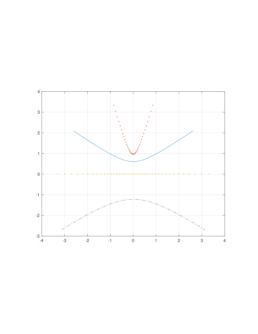
Figure 1. Example of curves ${\mathcal{L}}^{+}$ (solid line) and ${\mathcal{L}}^{-}$ (dash-dots). Example with $\lambda_{+}=1,\lambda_{-}=-2,\nu=1.2$. Dots: boundaries of the domain of analyticity around ${\mathcal{L}}^{+}$ used to derive the bound for the discretization error of the infinite trapezoid rule in the $y$-coordinate: dotted lines become straight lines $\{\operatorname{\rm Im}y=\pm d\}$.

See Fig. 1 for an example of the curves ${\mathcal{L}}^{\pm}_{\omega_{1},b,\omega}$. The integrals are efficiently evaluated making the change of variables $\xi=\chi_{\omega_{1},b,\omega}(y)$ and applying the simplified trapezoid rule.

Remark 2.1.

In the process of deformation, the expression $1+\psi(\xi)/q$ may not assume value zero. In order to avoid complications stemming from analytic continuation to an appropriate Riemann surface, it is advisable to ensure that $1+\psi(\xi)/q\not\in(-\infty,0]$. Thus, if $q>0$ - and only positive $q$’s are used in the Gaver-Stehfest method or GWR algorithm - and $X$ is a SL-process, any $\omega\in(0,\pi/2)$ is admissible in (2.15), and any $\omega\in(-\pi/2,0)$ is admissible in (2.16). If the sinh-acceleration is applied to the Bromwich integral, then additional conditions on $\omega$ must be imposed. See Sect. 4.3.

Remark 2.2.

In the remaining part of the paper, we assume that the Wiener-Hopf factors $\phi^{\pm}_{q}(\xi),q>0,$ admit the representations $\phi^{\pm}_{q}(\xi)=a^{\pm}_{q}+\phi^{\pm\pm}_{q}(\xi)$ and ${\mathcal{E}}^{\pm}_{q}=a^{\pm}_{q}I+{\mathcal{E}}^{\pm\pm}_{q}$, where $a^{\pm}_{q}\geq 0$, and $\phi^{\pm\pm}_{q}(\xi)$ satisfy the bounds

(2.17) $$|\phi^{+,+}_{q}(\xi)| \leq C_{+}(q)(1+|\xi|)^{-\nu_{+}},\ \operatorname{\rm Im}\xi\geq\mu_{-},$$

(2.18) $$|\phi^{-,-}_{q}(\xi)| \leq C_{+}(q)(1+|\xi|)^{-\nu_{-}},\ \operatorname{\rm Im}\xi\leq\mu_{+},$$

where $\nu_{\pm}>0$ and $C_{\pm}(q)>0$ are independent of $\xi$. These conditions are satisfied for all popular classes of Lévy processes bar the driftless Variance Gamma model. See Sect. A.1 for details.

3. Expectations of functions of the Lévy process and its extremum

3.1. Main theorems

Let $f$ be measurable and uniformly bounded on $U_{+}:=\{(x_{1},x_{2})\ |\ x_{2}\geq 0,x_{1}\leq x_{2}\}$. Fix $(x_{1},x_{2})\in U_{+}$. The function ${\mathbb{R}}_{+}\ni T\mapsto V(f;T;x_{1},x_{2})$ is measurable and uniformly bounded, hence, ${\tilde{V}}(f;q;x_{1},x_{2})$, the Laplace transform of $V(f;T;x_{1},x_{2})$ w.r.t. $T$, is a well-defined analytic function of $q$ in the right half-plane. Assuming that ${\tilde{V}}(f;q;x_{1},x_{2})$ is sufficiently regular, $V(f;T;x_{1},x_{2})$ can be represented by the Bromwich integral

(3.1) $$V(f;T;x_{1},x_{2})=\frac{1}{2\pi i}\int_{\operatorname{\rm Re}q=\sigma}e^{qT}{\tilde{V}}(f;q;x_{1},x_{2})\,dq,$$

where $\sigma>0$ is arbitrary. We derive an analytical representation for

$${\tilde{V}}(f;q;x_{1},x_{2})=q^{-1}{\mathbb{E}}[f(x_{1}+X_{T_{q}},\max\{x_{2},x_{1}+{\bar{X}}_{T_{q}}\})],$$

where $q>0$ and $T_{q}$ is an exponentially distributed random variable of mean $1/q$, independent of $X$, and prove that the resulting expression for ${\tilde{V}}(f;q;x_{1},x_{2})$ admits analytic continuation to the right half-plane. One can impose additional general conditions on $X$ and $f$ which ensure that ${\tilde{V}}(f;q;x_{1},x_{2})$ is sufficiently regular so that (3.1) holds. Such general conditions are either too messy or exclude some natural examples, for which the regularity can be established on the case-by-case basis. A standard trick which is used in [15, 14, 9] is as follows. Firstly, (3.1) holds in the sense of generalized functions. One integrates by parts in (3.1), and proves that the derivative ${\tilde{V}}_{q}(f;q;x_{1},x_{2})$ is of class $L_{1}$ as a function of $q$. Hence, $V(f;T;x_{1},x_{2})$ equals the RHS of (3.1) with $-T^{-1}{\tilde{V}}_{q}(f;q;x_{1},x_{2})$ in place of ${\tilde{V}}(f;q;x_{1},x_{2})$. After that, one proves that it is possible to integrate by parts back and obtain (3.1) for $T>0$. In examples that we consider, the integrands are of essentially the same form as in [15, 14, 9] for barrier options, and enjoy all properties that are used in [15, 14, 9] to justify (3.1).

In the theorem below, $I$ denotes the identity operator, $f_{+}$ is the extension of $f$ to ${\mathbb{R}}^{2}$ by zero, and $\Delta$ is the diagonal map: $\Delta(x)=(x,x)$.

Theorem 3.1.

Let $X$ be a Lévy process on ${\mathbb{R}}$, $q>0$, and let $f:U_{+}\to{\mathbb{R}}$ be a measurable and uniformly bounded function s.t. $(({\mathcal{E}^{-}_{q}}\otimes I)f)\circ\Delta:{\mathbb{R}}\to{\mathbb{R}}$ is measurable. Then

1. for any $x_{1}\leq x_{2}$,

   (3.2) $$q{\tilde{V}}(f;q;x_{1},x_{2}) = (({\mathcal{E}_{q}}\otimes I)f_{+})(x_{1},x_{2})+({\mathcal{E}^{+}_{q}}w(f;q,\cdot,x_{2}))(x_{1}),$$

   where

   (3.3) $$w(f;q,y,x_{2})={\bf 1}_{[x_{2},+\infty)}(y)((({\mathcal{E}^{-}_{q}}\otimes I)f_{+})(y,y)-(({\mathcal{E}^{-}_{q}}\otimes I)f_{+})(y,x_{2}));$$

2. the RHS’ of (3.2) and (3.3) admit analytic continuation w.r.t. $q$ to the right half-plane.

Proof.

By definition, part (a) of Lemma 2.1 amounts to the statement that the probability distribution of the ${\mathbb{R}}^{2}$-valued random variable $({\bar{X}}_{T_{q}},X_{T_{q}}-{\bar{X}}_{T_{q}})$ is equal to the product (in the sense of “product measure”) of the distribution of ${\bar{X}}_{T_{q}}$ and the distribution of $X_{T_{q}}-{\bar{X}}_{T_{q}}$. Applying Fubini’s theorem and then part (b), we derive for $x_{1}\leq x_{2}$

$${\mathbb{E}}[f_{+}(x_{1}+X_{T_{q}},\max\{x_{2},x_{1}+{\bar{X}}_{T_{q}}\})]$$

$$= {\mathbb{E}}[f_{+}(x_{1}+X_{T_{q}}-{\bar{X}}_{T_{q}}+{\bar{X}}_{T_{q}},\max\{x_{2},x_{1}+{\bar{X}}_{T_{q}}\})]$$

$$= {\mathbb{E}}[(({\mathcal{E}^{-}_{q}}\otimes I)f_{+})(x_{1}+{\bar{X}}_{T_{q}},\max\{x_{2},x_{1}+{\bar{X}}_{T_{q}}\})]$$

$$= {\mathbb{E}}[(({\mathcal{E}^{-}_{q}}\otimes I)f_{+})(x_{1}+{\bar{X}}_{T_{q}},x_{2})]$$

$$+{\mathbb{E}}[{\bf 1}_{x_{1}+\bar{X}_{T_{q}}\geq x_{2}}((({\mathcal{E}^{-}_{q}}\otimes I)f_{+})(x_{1}+{\bar{X}}_{T_{q}},x_{1}+{\bar{X}}_{T_{q}})-(({\mathcal{E}^{-}_{q}}\otimes I)f_{+})(x_{1}+{\bar{X}}_{T_{q}},x_{2}))].$$

Using (2.1), we write the first term on the rightmost side as $(({\mathcal{E}_{q}}\otimes I)f_{+})(x_{1},x_{2})$; the second term is the second term on the RHS of (3.2), which finishes the proof of (i). As operators acting in the space of bounded measurable functions, ${\mathcal{E}}^{\pm}_{q}$ admit analytic continuation w.r.t. $q$ to the right half-plane, which proves (ii). ∎

Remark 3.1.

The inverse Laplace transform of $q^{-1}({\mathcal{E}_{q}}\otimes I)f_{+}(x_{1},x_{2})$ equals ${\mathbb{E}}[f(x_{1}+X_{T},x_{2})]$, and, therefore, can be easily calculated using the Fourier transform technique and sinh-acceleration [29]. Essentially, we have the price of the European option of maturity $T$, the riskless rate being 0, depending on $x_{2}$ as a parameter. Thus, the new element is the calculation of the second term on the RHS of (3.2). We calculate both terms in the same manner in order to facilitate the explanation of various blocks of our method.

Theorem 3.2.

Let a Lévy process $X$ on ${\mathbb{R}}$, function $f:U_{+}\to{\mathbb{R}}$ and real $q>0$ satisfy the following conditions

1. there exist $\mu_{-}\leq 0\leq\mu_{+}$ such that $\forall$ $\gamma\in[\mu_{-},\mu_{+}]$, ${\mathbb{E}}[e^{-\gamma X_{1}}]<\infty$ and $q+\psi(i\gamma)>0$;

2. $f$ is a measurable function admitting the bound

   (3.4) $$|f(x_{1},x_{2})|\leq C(x_{2})e^{-\mu_{+}x_{1}},$$

   where $C(x_{2})$ is independent of $x_{1}\leq x_{2}$;

3. $(({\mathcal{E}^{-}_{q}}\otimes I)f)\circ\Delta$ is a measurable admitting the bound

   (3.5) $$|(({\mathcal{E}^{-}_{q}}\otimes I)f)(x_{1},x_{1})|\leq Ce^{-\mu_{-}x_{1}},$$

   where $C$ is independent of $x_{1}\geq 0$.

Then the statements (i)- (iii) of Theorem 3.1 hold.

Proof.

It suffices to consider non-negative $f$. Define $f_{n}(x_{1},x_{2})=\min\{n,f(x_{1},x_{2})\}$, $n=1,2,\ldots$. By the dominated convergence theorem, ${\tilde{V}}(f_{n};q;x_{1},x_{2})\uparrow{\tilde{V}}(f;q;x_{1},x_{2})$, a.s., and since $f_{n}$ is bounded, (3.2) holds with $f_{n}$ in place of $f$. We rewrite (3.2) in the form

$$q{\tilde{V}}(f;q;x_{1},x_{2}) = {\mathbb{E}}[(({\mathcal{E}^{-}_{q}}\otimes I)f_{+})(x_{1}+{\bar{X}}_{T_{q}},\bar{x}_{2}){\bf 1}_{x_{1}+\bar{X}_{T_{q}}<\bar{x}_{2}}]$$

$$+{\mathbb{E}}[(({\mathcal{E}^{-}_{q}}\otimes I)f_{+})(x_{1}+{\bar{X}}_{T_{q}},x_{1}+{\bar{X}}_{T_{q}}){\bf 1}_{x_{1}+\bar{X}_{T_{q}}\geq\bar{x}_{2}}],$$

and denote by ${\tilde{W}}_{1}(f_{n};q;x_{1},\bar{x}_{2})+{\tilde{W}}_{2}(f_{n};q;x_{1},\bar{x}_{2})$ the sum on the RHS of (3.1) with $f_{n}$ in place of $f$. Fix $x_{2}$. On the strength of (a) and (3.5), ${\tilde{W}}_{2}(f_{n};q;x_{1},\bar{x}_{2})$ admits a bound via $C{\mathcal{E}^{+}_{q}}e^{-\mu_{-}x_{1}}=C{\phi^{+}_{q}}(i\mu_{-})e^{-\mu_{-}x_{1}}$, where $C$ is independent of $n$. On the strength of (a) and (3.4), ${\tilde{W}}_{2}(f_{n};q;x_{1},\bar{x}_{2})$ admits a bound via $C(\bar{x}_{2}){\mathcal{E}^{+}_{q}}{\mathcal{E}^{-}_{q}}e^{-\mu_{+}x_{1}}=C_{1}(q,\bar{x}_{2})e^{-\mu_{+}x_{1}}$, where $C_{1}(q,\bar{x}_{2})$ is independent of $n$. Operators ${\mathcal{E}}^{\pm}_{q}$ being positive and bounded in $L_{\infty}$-spaces with weights $e^{\gamma x},\gamma\in[-\mu_{-},-\mu_{-}]$ (see Lemma 2.2, (v)), the limit of the RHSs of ${\tilde{W}}_{1}(f_{n};q;x_{1},x_{2})+{\tilde{W}}_{2}(f_{n};q;x_{1},x_{2})$ is finite and equal to the RHS of (3.1).

∎

Remark 3.2.

For functions of a Lévy process and its running infimum, results are mirror reflections of the results for a Lévy process and its supremum: change the direction of the real axis, and flip the lower and upper half-plane and operators ${\mathcal{E}}^{\pm}_{q}$.

Let $V(G;h;T;x)$ be the price of the barrier option with the payoff $G(X_{T})$ at maturity and no rebate if the barrier $h$ is crossed before or at time $n$; the rsikless rate is 0. Applying Theorem 3.2, we obtain the formula for the price of the single barrier options, which is equivalent to the formula derived in [13, 15, 16, 14] for wide classes of Lévy processes and generalized to all Lévy processes in [10]. The new version allows for more efficient numerical realizations.

Theorem 3.3.

Let the Lévy process $X$ on ${\mathbb{R}}$ and $q>0$ satisfy condition (a) of Theorem 3.2, and let $G$ be a measurable function admitting the bound $|G(x)|\leq C(e^{-\mu_{+}x}+e^{-\mu_{-}x})$, where $C$ is independent of $x\in{\mathbb{R}}$. Then, for $x<h$,

(3.7) $${\tilde{V}}(G;h;q,x)=q^{-1}({\mathcal{E}_{q}}G)(x)-q^{-1}({\mathcal{E}^{+}_{q}}{\bf 1}_{[h,+\infty)}{\mathcal{E}^{-}_{q}}G)(x).$$

3.2. Integral representation of the Laplace transform of the value function

In this Section, we assume that $q>0$. The RHS’ of the formulas for the Wiener-Hopf factors and formulas that we derive below admit analytic continuation w.r.t. $q$ so that the inverse Laplace transform can be applied. We assume that the representations ${\mathcal{E}}^{\pm}_{q}=a^{\pm}_{q}I+{\mathcal{E}}^{\pm,\pm}_{q}$ (see Remark 2.2 and Lemma A.1) hold. This excludes the driftless Variance Gamma model which requires a separate treatment. Using the equality

$$w(f;q,x_{1},x_{2})={\bf 1}_{[x_{2},+\infty)}(x_{1})((({\mathcal{E}^{-}_{q}}\otimes I)f_{+})(x_{1},x_{1})-(({\mathcal{E}^{-}_{q}}\otimes I)f_{+})(x_{1},x_{2}))=0,\quad x_{1}\leq x_{2},$$

we write the second term on the RHS of (3.2) as

(3.8) $$({\mathcal{E}^{+}_{q}}w(f;q,\cdot,x_{2}))(x_{1})=({\mathcal{E}}^{++}_{q}w(f;q,\cdot,x_{2}))(x_{1}).$$

Similarly, we rewrite (3.3) as

(3.9) $$w(f;q,y,x_{2})=a^{-}_{q}w_{0}(y,x_{2})+w^{-}(f;q,y,x_{2}),$$

where $w_{0}(y,x_{2})={\bf 1}_{[x_{2},+\infty)}(y)(f_{+}(y,y)-f_{+}(y,x_{2}))$, and

(3.10) $$w^{-}(f;q,y,x_{2})={\bf 1}_{[x_{2},+\infty)}(y)((({\mathcal{E}}^{--}_{q}\otimes I)f_{+})(y,y)-(({\mathcal{E}}^{--}_{q}\otimes I)f_{+})(y,x_{2})).$$

Substituting (3.9) into (3.8), we obtain

(3.11) $$({\mathcal{E}^{+}_{q}}w(f;q,\cdot,x_{2}))(x_{1})=c^{-}_{q}({\mathcal{E}}^{++}_{q}\otimes I)w_{0})(x_{1},x_{2})+(({\mathcal{E}}^{++}_{q}\otimes I)w^{-})(f;q,x_{1},x_{2}).$$

In order to derive explicit integral representations for the terms on the RHS of (3.11), we impose the following conditions, which can be relaxed:

1. condition (a) of Theorem 3.2 is satisfied;

2. there exist $\mu^{\prime}_{-},\mu^{\prime}_{+}\in(\mu_{-},\mu_{+})$, $\mu^{\prime}_{-}<\mu^{\prime}_{+}$ such that $f$ admits bounds

   (3.12) $$|f(x_{1},x_{2})| \leq C(x_{2})e^{-\mu^{\prime}_{+}x_{1}},\ x_{1}\leq x_{2},$$

   (3.13) $$|(({\mathcal{E}^{-}_{q}}\otimes I)f_{+})(x_{1},x_{1})| \leq Ce^{-\mu^{\prime}_{-}x_{1}},\ x_{1}\in{\mathbb{R}},$$

   where $C(x_{2})$ and $C$ are independent of $x_{1}\leq x_{2}$, and $x_{1}\in{\mathbb{R}}$, respectively;

3. for any $x_{2}$, there exists $C(x_{2})>0$ such that

   (3.14) $$|\widehat{(f_{+})}_{1}(\xi_{1},x_{2})| \leq C(x_{2})(1+|\xi_{1}|)^{-1},\quad\xi_{1}\in S_{[\mu^{\prime}_{+},\mu_{+}]},$$

   (3.15) $$|\widehat{(w_{0})}_{1}(\eta,x_{2})| \leq C(x_{2})(1+|\eta|)^{-1},\quad\eta\in S_{[\mu_{-},\mu^{\prime}_{-}]};$$

4. there exists $C>0$ such that for $\xi_{1}\in S_{[\mu^{\prime}_{+},\mu_{+}]}$ and $\xi_{2}\in S_{[\mu_{-},\mu^{\prime}_{-}]}$,

   (3.16) $$|\widehat{(f_{+})}(\xi_{1},\xi_{2})|\leq C(1+|\xi_{1}|)^{-1}(1+|\xi_{2}|)^{-1}.$$

Theorem 3.4.

Let conditions (a)-(d) hold and let the representations of the Wiener-Hopf factors in Remark 2.2 be valid. Then, for any $\omega,\omega_{1},\omega_{2}$ and $\omega_{-}$ satisfying

(3.17) $$\omega,\omega_{1}\in(\mu^{\prime}_{+},\mu_{+}),\ \omega_{2}\in(\mu_{-},\mu^{\prime}_{-}),\ \omega_{-}\in(\mu_{-},\omega_{1}+\omega_{2}),$$

and $x_{1}\leq x_{2}$, we have

$${\tilde{V}}(f;q;x_{1},x_{2}) = \frac{1}{2\pi}\int_{\operatorname{\rm Im}\xi=\omega}\frac{e^{ix_{1}\xi_{1}}}{q+\psi(\xi_{1})}\widehat{(f_{+})}(\xi_{1},x_{2})d\xi_{1}$$

$$+\frac{a^{-}_{q}}{2\pi q}\int_{\operatorname{\rm Im}\eta=\omega_{-}}e^{ix_{1}\eta}\phi^{++}_{q}(\eta)\widehat{(w_{0})}_{1}(\eta,x_{2})d\eta$$

$$+\frac{1}{2\pi q}\int_{\operatorname{\rm Im}\eta=\omega_{-}}e^{i(x_{1}-x_{2})\eta}\phi^{++}_{q}(\eta)\widehat{w^{-}_{0}}(f;q,\eta,x_{2})d\eta,$$

where $\widehat{w^{-}_{0}}(f;q,\eta,x_{2})$ is given by

$$\widehat{w^{-}_{0}}(f;q,\eta,x_{2})$$

$$= \frac{1}{2\pi}\int_{\operatorname{\rm Im}\xi_{1}=\omega_{1}}d\xi_{1}\,\frac{e^{ix_{2}\xi_{1}}}{i(\xi_{1}-\eta)}\phi^{--}_{q}(\xi_{1})(\widehat{f_{+}})_{1}(\xi_{1},x_{2})$$

$$+\frac{1}{(2\pi)^{2}}\int_{\operatorname{\rm Im}\xi_{1}=\omega_{1}}\int_{\operatorname{\rm Im}\xi_{2}=\omega_{2}}d\xi_{1}\,d\xi_{2}\,\frac{e^{ix_{2}(\xi_{1}+\xi_{2})}}{i(\eta-\xi_{1}-\xi_{2})}\phi^{--}_{q}(\xi_{1})(\widehat{f_{+}})(\xi_{1},\xi_{2}).$$

Proof.

The first term on the RHS of (3.2) is $(({\mathcal{E}_{q}}\otimes I)f_{+})(x_{1},x_{2})$, and the first term on the RHS of (3.4) is $q^{-1}(({\mathcal{E}_{q}}\otimes I)f_{+})(x_{1},x_{2})$. Consider the second term on the RHS of (3.2). We use (3.11). Since (3.15) holds and $\phi^{++}_{q}(\eta)=O(|\eta|^{-\nu_{+}})$ as $\eta\to\infty$ in the strip $S_{[\mu_{-},\mu_{+}]}$, where $\nu_{+}>0$, the integral

(3.20) $$(({\mathcal{E}}^{++}_{q}\otimes I)w_{0})(x_{1},x_{2})=\frac{1}{2\pi}\int_{\operatorname{\rm Im}\eta=\omega_{-}}e^{ix_{1}\eta}\phi^{++}_{q}(\eta)\widehat{(w_{0})}_{1}(\eta,x_{2})d\eta$$

is absolutely convergent. It remains to consider $({\mathcal{E}}^{++}_{q}w^{-}(f;q,\cdot,x_{2}))(x_{1})$. If $\operatorname{\rm Im}\eta=\omega_{-}$,

$$\widehat{w^{-}}(f;q,\eta,x_{2}) = -\int_{x_{2}}^{+\infty}dy\,e^{-iy\eta}\frac{1}{2\pi}\int_{\operatorname{\rm Im}\xi_{1}=\omega_{1}}d\xi_{1}\,e^{i\xi_{1}y}\phi^{--}_{q}(\xi_{1})(\widehat{f_{+}})_{1}(\xi_{1},x_{2})$$

$$+\int_{x_{2}}^{+\infty}dy\,e^{-iy\eta}\frac{1}{(2\pi)^{2}}\int_{\operatorname{\rm Im}\xi_{1}=\omega}\int_{\operatorname{\rm Im}\xi_{2}=\omega_{2}}d\xi_{1}\,d\xi_{2}\,e^{i(\xi_{1}+\xi_{2})y}\phi^{--}_{q}(\xi_{1})(\widehat{f_{+}})(\xi_{1},\xi_{2}).$$

We apply Fubini’s theorem to the first integral. The integral $\int_{x_{2}}^{+\infty}dy\,e^{i(-\eta+\xi_{1})y}=\frac{e^{ix_{2}(\xi_{1}-\eta)}}{i(\eta-\xi_{1})}$ converges absolutely since $-\omega_{-}+\omega_{1}>0$, and the repeated integral converges absolutely because $\phi^{--}_{q}(\xi)$ is uniformly bounded on the line of integration and (3.14) holds. Similarly, since $-\omega_{-}+\omega_{1}+\omega_{2}>0$, the integral $\int_{x_{2}}^{+\infty}dy\,e^{i(-\eta+\xi_{1}+\xi_{2})y}=e^{ix_{2}(\xi_{1}+\xi_{2}-\eta)}/(i(\eta-\xi_{1}-\xi_{2}))$ converges absolutely. Since $\phi^{--}_{q}(\xi)=O(|\xi_{1}|^{-\nu_{-}})$ as $\xi_{1}\to\infty$ along the line of integration, where $\nu_{-}>0$, (3.16) holds, and

(3.21) $$\int_{\mathbb{R}}\int_{\mathbb{R}}d\xi_{1}\,d\xi_{2}\,(1+|\xi_{1}+\xi_{2}|)^{-1}(1+|\xi_{1}|)^{-1-\nu_{-}}(1+|\xi_{2}|)^{-1}<\infty$$

(see Sect. A.2 for the proof), the Fubini’s theorem is applicable to the second integral as well. Thus,

(3.22) $$\widehat{w^{-}}(f;q,\eta,x_{2})=e^{-i\eta x_{2}}\widehat{w^{-}_{0}}(f;q,\eta,x_{2}),$$

where $\widehat{w^{-}_{0}}(f;q,\eta,x_{2})$ is given by (3.4), and we obtain the triple integral

(3.23) $$({\mathcal{E}}^{++}_{q}w^{-}(\cdot,x_{2}))(x_{1})=\frac{1}{2\pi}\int_{\operatorname{\rm Im}\eta=\omega_{-}}e^{i(x_{1}-x_{2})\eta}\phi^{++}_{q}(\eta)\widehat{w^{-}_{0}}(f;q,\eta,x_{2})d\eta.$$

The integrand admits a bound via $Cg(\eta,\xi_{1},\xi_{2})$, where

$$g(\eta,\xi_{1},\xi_{2})=(1+|\eta|)^{-\nu_{+}}(1+|\eta-\xi_{1}-\xi_{2}|)^{-1}(1+|\xi_{1}|)^{-1-\nu_{-}}(1+|\xi_{2}|)^{-1}.$$

Since

(3.24) $$\int_{{\mathbb{R}}^{3}}g(\eta,\xi_{1},\xi_{2})d\eta\,d\xi_{1}\,d\xi_{2}<\infty$$

(see Sect. A.2 for the proof), the triple integral on the the RHS of (3.23) is absolutely convergent. Substituting (3.11), (3.20) and (3.23) into (3.2), we obtain (3.4). ∎

Remark 3.3.

In standard situations such as in the two examples that we consider below, the function $y\mapsto h(y):=({\mathcal{E}}^{--}_{q}\otimes I)f_{+}(y,y)-({\mathcal{E}}^{--}_{q}\otimes I)f_{+}(y,x_{2})$ is a linear combination of exponential functions (with the coefficients depending on $x_{2}$). Then $\widehat{w^{-}}(q;\eta,x_{2})$ can be calculated directly, the double integral on the RHS of (3.4) can be reduced to 1D integrals, and the condition (3.16) replaced with the condition on $h$ similar to (3.15). Analogous simplifications are possible in more involved cases when $h$ is a piece-wise exponential polynomial in $y$.

3.3. Two examples

3.3.1. Example I. The joint cpdf of $X_{T}$ and ${\bar{X}}_{T}$

For $a_{1}\leq a_{2}$, and $x_{1}\leq x_{2}$, set $f(x_{1},x_{2})={\bf 1}_{(-\infty,\min\{a_{1},x_{2}\}]}(x_{1}){\bf 1}_{(-\infty,a_{2}]}(x_{2})$ and consider

$$V(f;T,x_{1},x_{2})={\mathbb{Q}}[x_{1}+X_{T}\leq a_{1},\max\{x_{2},x_{1}+{\bar{X}}_{T}\}\leq a_{2}].$$

If $x_{2}>a_{2}$, then $V(f;T,x_{1},x_{2})=0$. Hence, we assume that $x_{2}\leq a_{2}$.

Theorem 3.5.

Let $q>0$, $a_{1}\leq a_{2},x_{1}\leq x_{2}\leq a_{2}$, and let $X$ satisfy conditions of Theorem 3.4. Then, for any $\mu_{-}<\omega_{-}<0<\omega_{1}<\mu_{+}$,

$${\tilde{V}}(f;q,x_{1},x_{2})$$

$$= \frac{1}{2\pi}\int_{\operatorname{\rm Im}\xi_{1}=\omega_{1}}\frac{e^{i(x_{1}-a_{1})\xi_{1}}}{-i\xi_{1}(q+\psi(\xi_{1}))}d\xi_{1}$$

$$+\frac{1}{(2\pi)^{2}q}\int_{\operatorname{\rm Im}\eta=\omega_{-}}d\eta\,e^{i(x_{1}-a_{2})\eta}\phi^{++}_{q}(\eta)\int_{\operatorname{\rm Im}\xi_{1}=\omega_{1}}d\xi_{1}\,\frac{e^{i\xi_{1}(a_{2}-a_{1})}\phi^{--}_{q}(\xi_{1})}{\xi_{1}(\xi_{1}-\eta)}.$$

Proof.

We have $f_{+}(x_{1},x_{2})={\bf 1}_{(-\infty,a_{1}]}(x_{1}){\bf 1}_{(-\infty,a_{2}]}(x_{2}),$ therefore, for $x_{2}\leq a_{2}$,

$$w_{0}(y,x_{2}) = {\bf 1}_{[x_{2},+\infty)}(y){\bf 1}_{(-\infty,a_{1}]}(y)({\bf 1}_{(-\infty,a_{2}]}(y)-{\bf 1}_{(-\infty,a_{2}]}(x_{2}))$$

$$= -{\bf 1}_{[x_{2},+\infty)}(y){\bf 1}_{(-\infty,a_{1}]}(y){\bf 1}_{(a_{2},+\infty)}(y)=0,$$

hence, the second term on the RHS of (3.4) is 0. Next,

$$\widehat{(f_{+})}_{1}(\xi_{1},x_{2})={\bf 1}_{(-\infty,a_{2}]}(x_{2})\int_{-\infty}^{a_{1}}e^{-ix_{1}\xi_{1}}d\xi_{1}={\bf 1}_{(-\infty,a_{2}]}(x_{2})\frac{e^{-ia_{1}\xi_{1}}}{-i\xi_{1}}d\xi_{1}$$

is well-defined in the upper half-plane, and satisfies the bound (3.14) in any strip $S_{[\mu^{\prime}_{+},\mu_{+}]}$, where $\mu^{\prime}_{+}\in(0,\mu_{+})$. Hence, the first term on the RHS of (3.4) becomes the first term on the RHS of (3.5). It remains to evaluate the double integral on the RHS of (3.4). As mentioned in Remark 3.3, in the present case, it is simpler to directly evaluate $w^{-}$ and then $\widehat{w^{-}}$: for any $x_{2}\leq a_{2}$, $\omega_{1}\in(0,\mu_{+})$ and any $\eta\in\{\operatorname{\rm Im}\eta\in(\mu_{-},\omega_{1})\}$,

$$w^{-}(q,y,x_{2}) = {\bf 1}_{(x_{2},+\infty)}(y)({\mathcal{E}}^{--}_{q}{\bf 1}_{(-\infty,a_{1}]})(y)({\bf 1}_{(-\infty,a_{2}]}(y)-1)$$

$$= -{\bf 1}_{[a_{2},+\infty)}(y)({\mathcal{E}}^{--}_{q}{\bf 1}_{(-\infty,a_{1}]})(y)$$

$$= -{\bf 1}_{(a_{2},+\infty)}(y)\frac{1}{2\pi}\int_{\operatorname{\rm Im}\xi_{1}=\omega_{1}}d\xi_{1}\,e^{i(y-a_{1})\xi_{1}}\frac{\phi^{--}(\xi_{1})}{-i\xi_{1}},$$

$$\widehat{w^{-}}(q,\eta,x_{2}) = -\int_{a_{2}}^{+\infty}e^{-iy\eta}\frac{1}{2\pi}\int_{\operatorname{\rm Im}\xi_{1}=\omega_{1}}d\xi_{1}\,e^{i(y-a_{1})\xi_{1}}\frac{\phi^{--}(\xi_{1})}{-i\xi_{1}}$$

$$= -\frac{e^{-ia_{2}\eta}}{2\pi}\int_{\operatorname{\rm Im}\xi_{1}=\omega_{1}}d\xi_{1}\,e^{i(a_{2}-a_{1})\xi_{1}}\frac{\phi^{--}(\xi_{1})}{i(\eta-\xi_{1})(-i\xi_{1})}.$$

It is easy to see that both integrals are absolutely convergent. Substituting (3.3.1) into the double integral on the RHS of (3.4), we obtain (3.5). ∎

Remark 3.4.

If $x_{1}>a_{1}$, then it advantageous to move the line of integration in the first integral on the RHS of (3.5) down, and, on crossing the simple pole, apply the residue theorem. In the result, the first term on the RHS turns into

$$\frac{1}{q}+\frac{1}{2\pi}\int_{\operatorname{\rm Im}\eta=\omega_{-}}\frac{e^{i(x_{1}-a_{1})\eta}}{-i\eta(q+\psi(\eta))}d\eta.$$

Remark 3.5.

The first step of the proof of Theorem 3.5 implies that we can replace $\phi^{--}_{q}$ in the double integral on the RHS of (3.5) with ${\phi^{-}_{q}}$. From the computational point of view, if we make the conformal change of variables, this change does not lead to a significant increase in sizes of arrays necessary for accurate calculations, especially if $a_{2}-a_{1}>0$. The advantage is that it becomes unnecessary to evaluate $a^{-}_{q}$. Recall that the same $a^{-}_{q}$ appears for all $\xi_{1}$ in the formula $\phi^{--}_{q}(\xi_{1})={\phi^{-}_{q}}(\xi_{1})-a^{-}_{q}$, hence, it is necessary to evaluate $a^{-}_{q}$ with a higher precision that ${\phi^{-}_{q}}(\xi_{1})$. At the same time, the integrand in the formula for $a^{-}_{q}$ decays slower at infinity than the integrand in the formula for ${\phi^{-}_{q}}(\xi_{1})$, hence, a significantly longer grid is needed to evaluate ${\phi^{-}_{q}}(\xi_{1})$ sufficiently accurately.

Remark 3.6.

Denote by $I_{2}(q;x_{1},x_{2})$ the double integral on the RHS of (3.5) multiplied by $q$. It follows from (3.8) that we can replace $\phi^{++}_{q}$ in the double integral with ${\phi^{+}_{q}}$. If $a_{1}<a_{2}$ and the conformal deformations are used, then this replacement causes no serious computational problems. If $a_{1}=a_{2}$, then the replacement leads to errors typical for the Fourier inversion at points of discontinuity. However, in this case, the RHS of (3.5) can be simplified as follows. We replace $\phi^{\pm,\pm}_{q}$ with $\phi^{\pm}_{q}$, which is admissible, then push the line of integration in the inner integral down, cross two simple poles at $\xi_{1}=0$ and $\xi_{1}=\eta$, and apply the residue theorem. The double integral becomes the following 1D integral:

$$I_{2}(q;x_{1},x_{2})=\frac{1}{2\pi}\int_{\operatorname{\rm Im}\eta=\omega_{-}}d\eta\,e^{i(x_{1}-a_{2})\eta}\frac{{\phi^{+}_{q}}(\eta)(1-{\phi^{-}_{q}}(\eta))}{-i\eta}.$$

We push the line of integration to $\{\operatorname{\rm Im}\eta=\omega_{1}\}$ and use the equality ${\phi^{+}_{q}}(\eta){\phi^{-}_{q}}(\eta)=q/(q+\psi(\eta))$ to obtain the formula for the perpetual no-touch option:

(3.27) $$q{\tilde{V}}(f,q;x_{1},x_{2}) = \frac{1}{2\pi}\int_{\operatorname{\rm Im}\xi_{1}=\omega_{1}}d\xi_{1}\,\frac{e^{i(x_{1}-a_{2})\xi_{1}}{\phi^{+}_{q}}(\xi_{1})}{-i\xi_{1}},\ x_{1}\leq x_{2}\leq a_{2}.$$

Of course, (3.27) can be obtained using the main theorem directly.

Remark 3.7.

One can push the line of integration in the outer integral in the double integral on the RHS of (3.5) up and obtain

$$I_{2}(q;x_{1},x_{2}) = \frac{1}{4\pi}\int_{\operatorname{\rm Im}\xi_{1}=\omega_{1}}d\xi_{1}\,e^{i(x_{1}-a_{1})\xi_{1}}\frac{\phi^{++}_{q}(\xi_{1})\phi^{--}_{q}(\xi_{1})}{-i\xi_{1}}$$

$$+\frac{1}{(2\pi)^{2}}\mathrm{v.p.}\int_{\operatorname{\rm Im}\eta=\omega_{1}}d\eta\,e^{i(x_{1}-a_{2})\eta}\phi^{++}_{q}(\eta)\int_{\operatorname{\rm Im}\xi_{1}=\omega_{1}}d\xi_{1}\,\frac{e^{i\xi_{1}(a_{2}-a_{1})}\phi^{--}_{q}(\xi_{1})}{\xi_{1}(\xi_{1}-\eta)},$$

where $\mathrm{v.p.}$ denotes the Cauchy principal value. After that, one can apply the fast Hilbert transform. The integrand decaying very slowly at infinity, accurate calculations are possible only if very long grids are used, hence, the CPU cost is very large even for a moderate error tolerance.

3.3.2. Example II. Option to exchange the supremum for a power of the underlying

Let $\beta>1$. Consider the option to exchange the supremum $\bar{S}_{T}=e^{\bar{X}_{T}}$ for the power $S_{T}^{\beta}=e^{\beta X_{T}}$. The payoff function $f(x_{1},x_{2})=(e^{\beta x_{1}}-e^{x_{2}})_{+}{\bf 1}_{(-\infty,x_{2}]}(x_{1})$ satisfies (3.12)-(3.13) with arbitrary $\mu^{\prime}_{+}>0$, $\mu^{\prime}_{-}<-\beta$. In Sect. A.3, we prove

Proposition 3.6.

Let $\beta>1$ and let conditions of Theorem 3.4 hold with $\mu_{-}<-\beta,\mu_{+}>0$. Then, for $x_{1}\leq x_{2}$, and any $0<\omega_{1}<\mu_{+}$, $\mu_{-}<\omega_{-}<-\beta$,

(3.28) $${\tilde{V}}(f;q,x_{1},x_{2})=I_{1}(q,x_{1},x_{2})+q^{-1}\sum_{j=2,3}I_{j}(q,x_{1},x_{2}),$$

where $I_{j}(q,x_{1},x_{2})$, $j=1,2,3,$ are given by

(3.29) $$I_{1}(q,x_{1},x_{2})=\frac{1}{2\pi}\int_{\operatorname{\rm Im}\xi_{1}=\omega_{1}}d\xi_{1}\,\frac{e^{i(x_{1}-x_{2})\xi_{1}}}{q+\psi(\xi_{1})}\left(\frac{e^{x_{2}\beta}}{\beta-i\xi_{1}}+\beta\frac{e^{x_{2}(1+i\xi_{1}(1-1/\beta))}}{(\beta-i\xi_{1})(-i\xi_{1})}-\frac{e^{x_{2}}}{-i\xi_{1}}\right),$$

(3.30) $$I_{2}(q,x_{1},x_{2})=a^{-}_{q}\frac{e^{x_{2}}}{2\pi}\int_{\operatorname{\rm Im}\eta=\omega_{-}}d\eta\,e^{i(x_{1}-x_{2})\eta}\frac{\phi^{++}_{q}(\eta)}{i\eta(1-i\eta)},$$

$$I_{3}(q,x_{1},x_{2})$$

$$= \frac{1}{(2\pi)^{2}}\int_{\operatorname{\rm Im}\eta=\omega_{-}}d\eta\,e^{i(x_{1}-x_{2})\eta}\phi^{++}_{q}(\eta)\int_{\operatorname{\rm Im}\xi_{1}=\omega_{1}}d\xi_{1}\,e^{-ix_{2}\xi_{1}}\frac{\phi^{--}_{q}(\xi_{1})}{i(\eta-\xi_{1})}$$

$$\cdot\left[\frac{e^{\beta x_{2}}}{i\eta-\beta}+\frac{\beta e^{(1+i\xi_{1}(1-1/\beta)x_{2}}(1-i\xi_{1}/\beta)}{(\beta-i\xi_{1})(-i\xi_{1})(i\eta-1-i\xi_{1}(1-1/\beta))}-\frac{e^{x_{2}}(1-i\xi_{1})}{(-i\xi_{1})(i\eta-1)}\right].$$

4. Numerical evaluation of $V(f;T;x_{1},x_{2})$ in Example I

4.1. Standing assumption

In this section, we assume that $X$ is a SINH-regular process of order $\nu\in[0+,2]\setminus\{1+\}$ and type $([\mu_{-},\mu_{+}],{\mathcal{C}}_{\gamma_{-},\gamma_{+}},{\mathcal{C}}_{\gamma^{\prime}_{-},\gamma^{\prime}_{+}})$, where $\mu_{-}<0<\mu_{+}$ and $\gamma^{\prime}_{-}<0<\gamma^{\prime}_{+}$. Furthermore, we assume that either $\nu\geq 1$ or $\nu<1$ and the “drift” $\mu$ in (2.5) is 0. Then

(4.1) $$\operatorname{\rm Re}\psi(\xi)\geq c_{\psi;\infty}|\xi|^{\nu}-C_{\psi},\quad\forall\,\xi\in i(\mu_{-},\mu_{+})+({\mathcal{C}}_{\gamma^{\prime}_{-},\gamma^{\prime}_{+}}\cup\{0\}),$$

where $C_{\psi},c_{\psi;\infty}>0$ are independent of $\xi$.

Lemma 4.1.

Let the characteristic exponent $\psi$ of a SINH-regular process satisfy (4.1).

Then there exist $\omega_{\ell}\in(0,\pi/2)$ and $c,\sigma>0$ such that for all $q\in\sigma+{\mathcal{C}}_{\pi/2+\omega_{\ell}}$ and $\xi\in i(\mu_{-},\mu_{+})+({\mathcal{C}}_{\gamma^{\prime}_{-},\gamma^{\prime}_{+}}\cup\{0\})$,

(4.2) $$|q+\psi(\xi)|\geq c(|q|+|\xi|^{\nu}).$$

Proof.

Since $\psi(\xi)$ admits an upper bound via $C(1+|\xi|^{\nu})$, condition (4.1) implies that there exist $C_{1}>0$ and $\gamma\in(0,\pi/2)$ such that $\psi(\xi)+C_{1}\in{\mathcal{C}}_{\gamma}$ for all $\xi\in i(\mu_{-},\mu_{+})+({\mathcal{C}}_{\gamma^{\prime}_{-},\gamma^{\prime}_{+}}\cup\{0\})$. Hence, for any $\omega_{\ell}\in(0,\pi/2-\gamma)$, there exist $\sigma,c>0$ such that (4.2) holds.

∎

The bound (4.2) allows us to use one sinh-deformed contour in the lower half-plane and one in the upper half-plane for all purposes: the calculation of the Wiener-Hopf factors and evaluation of the integrals on the RHS of (3.5). If either $\mu_{-}=0$ or $\mu_{+}=0$, then both contours must cross $i{\mathbb{R}}$ in the same half-plane but the types of contours (two non-intersecting contours, one with the wings deformed upwards, the other one with the wings deformed downwards) remain the same as in the case $\mu_{-}<0<\mu_{+}$.

If (4.1) fails, for instance, if $\nu<1$ and $\mu\neq 0$, then the contour of integration in the formulas for the Wiener-Hopf factors can be deformed only upwards (if $\mu>0$) or downwards (if $\mu<0$). A similar complication arises if $\nu=1+$. For instance, for KoBoL of order 1+ in the asymmetric case $c_{+}\neq c_{-}$, the type of admissible deformations depends on the sign of $c_{1}-c_{2}$. Hence, we need to use an additional contour to evaluate the Wiener-Hopf factors. Even more importantly, the conformal deformations can be used only if the Gaver-Stephest method or GWR algorithm are used or the line of integration in the Bromwich integral is not deformed; conformal deformations of the contours of integration in the formula for ${\tilde{V}}(f;q,x_{1},x_{2})$ and the Bromwich integral are impossible if we want to preserve the analyticity of the double and triple integrands. To see this, it suffices to consider the degenerate case $\psi(\xi)=-i\mu\xi$: the conditions $q-i\mu\xi_{1}\not\in(0,\infty]$, $q-i\mu\eta\not\in(0,\infty]$ are impossible to satisfy if $\operatorname{\rm Re}q\to-\infty$, and the $\xi_{1}$- and $\eta$- contours are deformed upward and downward. Hence, we can either use the Gaver-Wynn Rho algorithm (see Sect. A.7) or acceleration schemes of the Euler type, e.g., the summation by parts formula (see Sect. A.6). See Sect. A.8 for details. Finally, if either $\gamma^{\prime}_{-}=0$ or $\gamma^{\prime}_{+}=0$ (but not both), then additional complications arise, and some of deformations have to be of a less efficient sub-polynomial type. See [30] for examples in the context of calculation of stable probability distributions.

4.2. Sinh-acceleration

Consider the first term on the RHS of (3.5), denote it $I_{1}(q;x_{1}-a_{1})$. As $\xi\to\infty$ along the line of integration, the integrand decays not faster than $|\xi|^{-3}$. The error of the truncation $\sum_{|j|\leq N}$ of the infinite sum $\sum_{j\in{\mathbb{Z}}}$ in the infinite trapezoid rule is approximately equal to the error of the truncation $\int_{-\Lambda}^{\Lambda}$, $\Lambda=N\zeta$, of the integral $\int_{-\infty}^{+\infty}$, hence, for a small error tolerance $\epsilon>0$, $\Lambda$ must be of the order of $\epsilon^{-1/2}$, and the complexity of the numerical scheme of the evaluation of the integral is of the order of $\epsilon^{-1/2}\ln(1/\epsilon)$. If $x_{1}-a_{1}$ is not small in absolute value, acceleration schemes of the Euler type can be employed to decrease the number of terms of the simplified trapezoid rule. If $x_{1}-a_{1}$ is zero or very close to 0, Euler acceleration schemes are either non-applicable or rather inefficient.

Let $X$ be SINH-regular. Assuming that in Definition 2.3, $\gamma_{\pm}$ are not extremely small in absolute value, the sinh-acceleration (2.14) is the most efficient change of variables. Note that in (2.14), $\omega_{1}\in{\mathbb{R}}$ is, generally, different from $\omega_{1}$ in the formulas of the preceding sections, $\omega\in(-\pi/2,\pi/2)$ and $b>0$. The parameters $\omega_{1},b,\omega$ are chosen so that the contour ${\mathcal{L}}_{\omega_{1},b,\omega}:=\chi_{\omega_{1},b,\omega}({\mathbb{R}})\subset i(0,\mu_{+})+({\mathcal{C}}_{\gamma_{-},\gamma_{+}}\cup\{0\})$. The parameter $\omega$ is chosen so that the oscillating factor becomes a fast decaying one. Under the integral sign of the integral $I_{1}(q;x_{1}-a_{1})$, the oscillating factor is $e^{i(x_{1}-a_{1})\xi_{1}}$. Hence, if $x_{1}<a_{1}$, we must choose $\omega\in(\gamma^{\prime}_{-},0)$ (an approximately optimal choice is $\omega=\gamma^{\prime}_{-}/2$), if $x_{1}-a_{1}>0$, we must choose $\omega\in(0,\gamma^{\prime}_{+})$ (an approximately optimal choice is $\omega=\gamma^{\prime}_{+}/2$), and if $x_{1}=a_{1}$, any $\omega\in(\gamma^{\prime}_{-},\gamma^{\prime}_{+})$ is admissible (an approximately optimal choice is $\omega=(\gamma^{\prime}_{-}+\gamma^{\prime}_{+})/2$). If $x_{1}-a_{1}<0$, it is advantageous to push the line of integration in the 1D integral to the lower half-plane, and, on crossing the simple pole at 0, apply the residue theorem.

To evaluate the repeated integral on the RHS of (3.5), we deform both lines of integration. Since $a_{2}-a_{1}>0$, it is advantageous to deform the wings of the contour of integration w.r.t. $\xi_{1}$ up; denote this contour ${\mathcal{L}}^{+}:={\mathcal{L}}_{\omega^{+}_{1},b^{+},\omega^{+}}$. Since $x_{1}-a_{2}\leq 0$, it is advantageous to deform the wings of the contour of integration w.r.t. $\eta$ down, denote this contour ${\mathcal{L}}^{-}:={\mathcal{L}}_{\omega^{-}_{1},b^{-},\omega^{-}}$. Hence, we choose $\omega^{+}=\gamma^{\prime}_{+}/2$, $\omega^{-}=\gamma^{\prime}_{-}/2$; the remaining parameters are chosen so that $\mu_{+}>\omega^{+}_{1}+b^{+}\sin\omega^{+}>0>\omega^{-}_{1}+b^{-}\sin\omega^{-}>\mu_{-}$. See Fig. 1. The result is

$${\tilde{V}}(f;q,x_{1},x_{2}) = \frac{1}{2\pi}\int_{{\mathcal{L}}_{\omega_{1},b,\omega}}\frac{qe^{i(x_{1}-a_{1})\xi_{1}}}{(q+\psi(\xi_{1}))(-i\xi_{1})}d\xi_{1}$$

$$+ \frac{1}{(2\pi)^{2}q}\int_{{\mathcal{L}}^{-}}d\eta\,e^{i(x_{1}-a_{2})\eta}{\phi^{+}_{q}}(\eta)\int_{{\mathcal{L}}^{+}}d\xi_{1}\,\frac{e^{i\xi_{1}(a_{2}-a_{1})}{\phi^{-}_{q}}(\xi_{1})}{\xi_{1}(\xi_{1}-\eta)}.$$

We make an appropriate sinh-change of variables in each integral, and apply the simplified trapezoid rule w.r.t. each new variable.

4.3. Calculations using the sinh-acceleration in the Bromwich integral

Define

(4.4) $$\chi_{L;\sigma_{\ell},b_{\ell},\omega_{\ell}}(y)=\sigma_{\ell}+ib_{\ell}\sinh(i\omega_{\ell}+y),$$

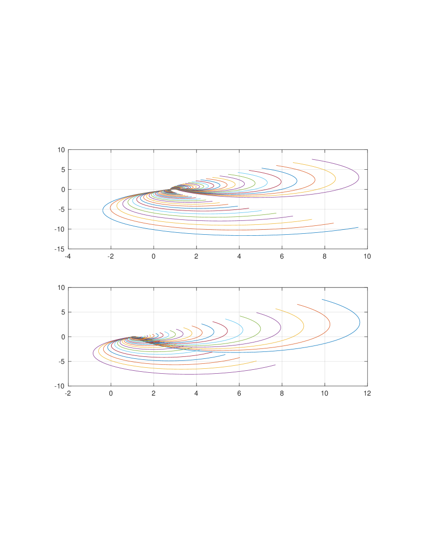
Figure 2. Plots of curves $\eta\mapsto 1+\psi(\eta)/q$, for $q$ in the SINH-Laplace inversion and $\eta$ on the contours ${\mathcal{L}}^{\pm}$ (upper and lower panels) in the numerical example with $\nu=1.2$.

where $\omega_{\ell}\in(0,\pi/2),b_{\ell}>0,\sigma_{\ell}-b_{\ell}\sin\omega_{\ell}>0$, and deform the line of integration in the Bromwich integral to ${\mathcal{L}}^{(L)}=\chi_{L;\sigma_{\ell},b_{\ell},\omega_{\ell}}(R)$. For $q\in{\mathcal{L}}^{(L)}$, we can calculate ${\tilde{V}}(f;q,x_{1},x_{2})$ using the same algorithm as in the case $q>0$, if there exist $R,q_{0},\gamma>0$ and $\gamma_{--}<0<\gamma_{++}$ such that $q+\psi(\eta)\neq 0$ for all $q\in{\mathcal{L}}^{(L)}$ and $\eta\in{\mathcal{C}}_{\gamma_{--},\gamma_{++}},|\eta|\geq R$. In order to avoid the complications of the evaluation of the logarithm on the Riemann surface, it is advisable to ensure that $1+\psi(\eta)/q\not\in(-\infty,0]$ for pairs $(q,\eta)$ used in the numerical procedure. See Fig. 2 for an illustration. These conditions can be satisfied if (4.1) holds.

The sequence of deformations is as follows. First, for $q$ on the line of integration $\{\operatorname{\rm Im}q=\sigma\}$ in the Bromwich integral, we deform the contours of deformation w.r.t. $\eta$ and $\xi_{1}$ (and contours in the formulas for the Wiener-Hopf factors). Then we deform the line of integration w.r.t. $q$ into the contour ${\mathcal{L}}^{(L)}$. We choose $\omega_{\ell}$ and $\omega^{\pm}$ sufficiently small in absolute value so that, in the process of deformation, for all $1+\psi(\xi)/q\neq 0$ and $q+\psi(\eta)/q\neq 0$ for all dual variables $q,\eta,\xi_{1}$ that appear in the formulas for ${\tilde{V}}(f;q;x_{1},x_{2})$ and formulas for the Wiener-Hopf factors. To make an appropriate choice, the bound (4.1) must be taken into account. See [25] for details. In [25], fractional-parabolic deformations and changes of variables were used. The modification to the sinh-acceleration is straightforward.

4.4. The main blocks of the algorithm

For the sake of brevity, we omit the block for the evaluation of the 1D integral on the RHS of (3.5); this block is the same as in the European option pricing procedure (see [29]); the type of deformation depends on the sign of $x_{1}-a_{1}$. For the 2D integral, the scheme is independent of $x_{1}-a_{1}$. We formulate the algorithm assuming that the sinh-acceleration is applied to the Bromwich integral; if the Gaver-Wynn Rho algorithm is used, the modifications of the first step and last step are described in Sect. A.7. We calculate $F(T,a_{1},a_{2})=V(T,a_{1},a_{2};0,0)$ (that is, $x_{1}=x_{2}=0$).

1. Choose the sinh-deformation in the Bromwich integral and grid for the simplified trapezoid rule: $\vec{y}=\zeta_{\ell}*(0:1:N_{\ell})$, $\vec{q}=\sigma_{\ell}+i*b_{\ell}*\sinh(i*\omega_{\ell}+\vec{y})$. Calculate the derivative $\vec{der_{\ell}}=i*b_{\ell}*\cosh(i*\omega_{\ell}+\vec{y})$.

2. Choose the sinh-deformations and grids for the simplified trapezoid rule on ${\mathcal{L}}^{\pm}$: $\vec{y^{\pm}}=\zeta^{\pm}*(-N^{\pm}:1:N^{\pm})$, $\vec{\xi^{\pm}}=i*\omega_{1}^{\pm}+b^{\pm}*\sinh(i*\omega^{\pm}+i\vec{y^{\pm}})$. Calculate $\vec{\psi^{\pm}}=\psi(\vec{\xi^{\pm}})$ and $\vec{der^{\pm}}=b^{\pm}*\cosh(i*\omega^{\pm}+\vec{y^{\pm}}).$

3. Calculate the matrices $D^{+}=[1/(\xi^{+}_{j}-\xi^{-}_{k})]$ and $D^{-}=[1/(\xi^{-}_{k}-\xi^{+}_{j})]$ (the sizes are $(2*N^{+}+1)\times(2*N^{-}+1)$ and $(2*N^{-}+1)\times(2*N^{+}+1)$, respectively).

4. The main block (the same block is used if the Gaver-Wynn Rho algorithm is applied). For given $x_{1},x_{2},a_{1},a_{2}$, in the cycle in $q\in\vec{q}$, evaluate

   1. ${\phi^{+}_{q}}$ at points of the grid ${\mathcal{L}}^{+}$ and ${\phi^{-}_{q}}$ at points of the grid ${\mathcal{L}}^{-}$ using (2.15)-(2.16):

      $$\vec{\phi^{\pm}_{q}}=\exp\left[((\mp\zeta^{\pm}*i/(2*\pi))*\vec{\xi^{\pm}}.*(\log(1+\vec{\psi^{\mp}}/q)./\vec{\xi^{\mp}}.*\vec{der^{\mp}})*D^{\pm})\right];$$

   2. calculate $\phi^{\pm}_{q}$ at points of the grid ${\mathcal{L}}^{\mp}$: $\vec{\phi^{\pm}_{q,\mp}}=q./(q+\vec{\psi^{\mp}})./\vec{\phi^{\mp}_{q}};$

   3. evaluate the 2D integral on the RHS of (3.5)

      $$Int2(q) = ((\zeta^{-}*\zeta^{+}/(2*\pi)^{2})*(\exp(-i*a_{2}*\vec{\xi^{-}}).*\vec{\phi^{+}_{q,-}}.*\vec{der^{-}})*D^{+})$$

      $$*\mathrm{conj}((\exp((i*(a_{2}-a_{1}))*\vec{\xi^{+}}).*\vec{\phi^{-}_{q,+}}/\vec{\xi^{+}}.*\vec{der^{+}})^{\prime}).$$

   4. depending on the sign of $x_{1}-a_{1}$, use either the arrays $\vec{\xi^{+}},\vec{der^{+}},\vec{\psi^{+}}$ or $\vec{\xi^{-}},\vec{der^{-}},\vec{\psi^{-}}$ to evaluate $Int1(q)$, the 1D integral on the RHS of (4.2).

5. Laplace inversion. Set $Int(\vec{q})=Int2(\vec{q})./\vec{q}+Int1(\vec{q})$, $Int(q_{1})=Int(q_{1})/2$, and, using the symmetry $\overline{{\tilde{V}}(q)}={\tilde{V}}(\bar{q})$, calculate

   $$V=(\zeta_{\ell}/\pi)*\mathrm{real}(\mathrm{sum}(\exp(T*\vec{q}).*Int(\vec{q}).*\vec{der_{\ell}})).$$

4.5. Numerical examples

Numerical results are produced using Matlab R2017b on MacBook Pro, 2.8 GHz Intel Core i7, memory 16GB 2133 MHz. The CPU times reported below can be significantly improved because

1. the main block of the program, namely, evaluation of ${\tilde{V}}(q)$ for a given array of $(a_{1},a_{2})$, is used both for complex and positive $q$’s. However, if $q>0$, we can use the well-known symmetries to decrease the sizes of arrays, hence, the CPU time. Furthermore, the block admits the trivial parallelization;

2. we use the same grids for the calculation of the Wiener-Hopf factors $\phi^{\pm}_{q}$ and evaluation of integrals on the RHS of (4.2). However, $\phi^{\pm}_{q}$ need to be evaluated only once and used for all points $(a_{1},a_{2})$. But if $x_{1}-a_{2}$ and $a_{2}-a_{1}$ are not very small in absolute value, then much shorter grids can be used to evaluate the integrals on the RHS of (3.5). See examples in [26, 56, 29, 31]. Therefore, if the arrays $(x_{1}-a_{2},a_{2}-a_{1})$ are large, then the CPU time can be decreased using shorter arrays for calculation of the integrals on the RHS of (4.2).

3. If the values $F(T,a_{1},a_{2})$ are needed for several values of $T$ in the range $[T_{1},T_{2}]$, where $T_{1}$ is not too close to 0 and $T_{2}$ is not too large, then the CPU time can be significantly decreased applying the sinh-acceleration to the Bromwich integral. Indeed, the main step is time independent, and the last step, which is the only step where $T$ appears, admits an easy parallelization. Hence, the CPU time for many values of $T$ is essentially the same as for one value of $T$.

Item (a), and, partially, (b) are motivated by our aim to compare the performance of the algorithm based on the Gaver-Wynn Rho algorithm and the one based on the sinh-acceleration applied to the Bromwich integral. Since the same subprogram for the evaluation of ${\tilde{V}}(q)$ is used in both cases, and, even in the more complicated second case, we can achieve the precision of the order of $E-14$, we can safely say that the errors in the first case are the errors of the Gaver-Wynn Rho algorithm itself; and these errors are of the order of $E-7$ in the cases we considered (sometimes, larger, in other cases, somewhat smaller), which agrees with the general empirical observation $(E-0.9)M$, for all choices of the parameters of the numerical scheme. The errors remain essentially the same even if we use much finer and longer grids in the $\eta$- and $\xi$-spaces than it is necessary. The second motivation for (b) is that we wish to give a relatively short description of the choice of the main parameters of the numerical scheme.

In the two examples that we consider, $X$ is KoBoL with the characteristic exponent $\psi(\xi)=c\Gamma(-\nu)(\lambda_{+}^{\nu}-(\lambda_{+}+i\xi)^{\nu}+(-\lambda_{-})^{\nu}-(-\lambda_{-}-i\xi)^{\nu})$, where $\lambda_{+}=1,\lambda_{-}=-2$ and (I) $\nu=0.2$, hence, the process is close to Variance Gamma; (II) $\nu=1.2$, hence, the process is close to NIG. In both cases, $c>0$ is chosen so that the second instantaneous moment $m_{2}=\psi^{\prime\prime}(0)=0.1$. For $X_{0}={\bar{X}}_{0}=0$, we calculate the joint cpdf $F(T,a_{1},a_{2}):=V(T,a_{1},a_{2};0,0)$ for $T=0.25$ in Case (I) and for $T=0.05,0.25,1,5,15$ in Case (II). In both cases, $a_{1}$ is in the range $[-0.075,0.1]$ and $a_{2}$ in the range $[0.025,0.175]$; the total number of points $(a_{1},a_{2})$, $a_{1}\leq a_{2}$, is 44. The parameters of the numerical schemes are chosen as follows.

For SL-processes, and KoBoL is an SL-process, any sinh-deformation is admissible provided is a subset of $i(\mu^{\prime}_{-},\mu^{\prime}_{+})+({\mathcal{C}}_{+}\cup\{0\})$ and $q_{1}+\psi(i(\omega_{1}-b\sin(\omega))>0$ for the smallest $q=q_{1}>0$ used in the Gaver-Wynn Rho algorithm. IIf $q_{1}+\psi(i(\omega_{1}-b\sin(\omega))\leq 0$ then we can reduce the calculations to the case $q_{1}+\psi(i(\omega_{1}-b\sin(\omega))>0$ crossing the purely imaginary zero of $q+\psi(\xi)$ as in [57]. In the examples that we consider, $q_{1}+\psi(i(\omega_{1}-b\sin(\omega))>0$.

For SL-processes, the choice of the most important parameters $\omega^{\pm}$ trivializes: $\omega^{\pm}=\pm\pi/4\cdot\min\{1,1/\nu\}$, and the half-width $d^{\pm}$ of the strips of analyticity in the new coordinates is $d=|\omega^{\pm}|$. It can be easily shown that, for the Merton model and Meixner processes, one can choose $\omega^{\pm}=\pm\pi/8$ and $d^{\pm}=|\omega^{\pm}|$ (see [35] for the analysis of the domain of analyticity and zeros of $q+\psi(\xi)$ for popular Lévy models). Thus, given the error tolerance $\epsilon$, we can easily write a universal approximate recommendation for the choice of $\zeta$. The recommendation for an approximately optimal choice of the truncation parameter $\Lambda=N\zeta$ is the same as in [31]. As in [31], typically, the recommendation leads to grids somewhat longer than necessary. Choosing the parameters by hand, we observe that the results with the errors of the order of E-7, which are inevitable with the Gaver-Wynn Rho algorithm, can be achieved using the sinh-acceleration in the $\xi$- and $\eta$-spaces, with grids of the length 100 or even smaller (depending on $\nu$ and $T$). If the calculations are made using the Hilbert transform or simplified trapezoid rule without the conformal deformations, then much longer arrays will be needed (thousand times longer and more) to satisfy even larger error tolerance, and the increase of the speed due to the use of the fast Hilbert transform or fast convolution and fast inverse Fourier transform cannot compensate for the very large increase of the sizes of the arrays.

If the sinh-acceleration in the Bromwich integral is used, then we can satisfy the error tolerance of the order E-14 and smaller using the $q$-grids of the order of 100-150, and the $\xi$- and $\eta$-grids of the order of $250-450$. We use two types of deformations: (I) $\omega_{\ell}=(\pi/2)/9,\omega_{\pm}=\pm(\pi/2)/4.5\cdot\min\{1,1/\nu\}$ (“+” for ${\mathcal{L}}^{+}$, “-” for ${\mathcal{L}}^{-}$) and (II) $\omega_{\ell}=(\pi/2)/10,\omega_{\pm}=\pm(\pi/2)/5\cdot\min\{1,1/\mu\}$. Since each of the three curves has changed, the probability of a random agreement between the two results is negligible. The differences being less than $E-14$, with some exceptions in the case $T=15$, we take these values as the benchmark. The errors in Tables 1 and 2 are calculated w.r.t. the benchmark probabilities. The CPU time for the benchmark probabilities is in the range 5-8 msec, for one pair $(a_{1},a_{2})$, and 35-60 msec for 44 points (average of 100 runs). Choosing the parameters by hand, we calculated prices with errors somewhat smaller than the errors of the Gaver-Wynn Rho algorithm. The $\xi$- and $\eta$-grids can be chosen shorter than in the case of the Gaver-Wynn Rho algorithm but the length of the $q$-grid is several times larger than 16 in the Gaver-Wynn Rho algorithm; the CPU time is several times larger.

Table 1. Joint cpdf $F(T,a_{1},a_{2}):={\mathbb{Q}}[X_{T}\leq a_{1},{\bar{X}}_{T}\leq a_{2}\ |\ X_{0}={\bar{X}}_{0}=0]$, and errors (rounded) and CPU time (in msec) of two numerical schemes. KoBoL close to Variance Gamma, with an almost symmetric jump density, and no “drift”: $m_{2}=0.1$, $\nu=0.2,\lambda_{-}=-2,\lambda_{+}=1,\mu=0$; $T=0.25$.

$a_{2}/a_{1}$	-0.075	-0.05	-0.025	0	0.025
0.025	0.0528532412024316	0.0649856679446115	0.0879014169039594	0.506498701211732	0.923417160799499
0.05	0.0533971065051705	0.0656207900757611	0.088669961239051	0.507497961893707	0.925278586629321
0.075	0.0536378889312989	0.0658957955144874	0.0889908892581364	0.50788584329118	0.925781540582069
0.1	0.0537738608706033	0.0660488001673674	0.0891656084917816	0.508089681056682	0.926027783268806
0.175	0.0539603399744032	0.0662551510091744	0.0893960371866527	0.508350135593748	0.92632726895684

			$A$					B
$a_{2}/a_{1}$	-0.075	-0.05	-0.025	0	0.025	-0.075	-0.05	-0.025	0	0.025
0.025	-1.3E-08	-1.4E-08	-2.0E-08	1.6E-05	1.5E-08	6.9E-11	4.6E-11	6.1E-11	9.5E-08	4.5E-09
0.05	-1.4E-08	-1.4E-08	-1.9E-08	3.5E-05	1.0E-08	4.67E-11	1.9E-11	2.7E-11	9.5E-08	2.5E-09
0.075	-1.4E-08	-1.4E-08	-1.8E-08	-2.7E-05	1.0E-08	3.8E-11	9.2E-12	1.6E-11	9.5E-08	2.5E-09
0.1	-1.4E-08	-1.3E-08	-1.7E-08	-6.9E-06	1.0E-08	3.7E-11	8.6E-12	1.5E-11	9.5E-08	2.5E-09
0.175	-1.3E-08	-1.3E-08	-1.6E-08	-7.1E-07	1.1E-08	3.3E-11	3.9E-12	9.7E-12	9.5E-08	2.5E-09

Errors of the benchmark values: better than e-14. CPU time per 1 point: 118, per 44 points: 1,089.
A: Gaver-Wynn Rho algorithm, $2M=16$, $N^{\pm}=110$. CPU time per 1 point: 6.4; per 44 points: 44.3.
B: SINH applied to the Bromwich integral, with $N_{\ell}=65,N^{\pm}=91$. CPU time per 1 point 13.3, per 44 points: 175.
If in A, $N^{\pm}=115$ instead of $N^{\pm}=110$ are used, the rounded errors do not change but the CPU time increases.

Table 2. Errors (rounded) and CPU time (in msec) of two numerical schemes for the calculation of the joint cpdf $F(T,a_{1},a_{2}):={\mathbb{Q}}[X_{T}\leq a_{1},{\bar{X}}_{T}\leq a_{2}\ |\ X_{0}={\bar{X}}_{0}=0]$; $T=0.25$. KoBoL close to NIG, with an almost symmetric jump density, and no “drift”: $m_{2}=0.1$, $\nu=1.2,\lambda_{-}=-2,\lambda_{+}=1$. The benchmark values (for $T=0.05,0.25,1,5,15$) are in Table 3 in Section B.

			$A$					B
$a_{2}/a_{1}$	-0.075	-0.05	-0.025	0	0.025	-0.075	-0.05	-0.025	0	0.025
0.025	2.6E-07	2.3E-06	-1.1E-06	-3.1E-06	4.0E-06	5.3E-09	7.5E-09	1.1E-08	1.6E-08	2.8E-08
0.05	1.5E-06	3.9E-06	-4.9E-06	2.6E-07	2.4E-06	1.7E-09	2.3E-09	3.3E-09	5.3E-09	8.0E-09
0.075	2.1E-06	4.8E-06	1.9E-07	-1.4E-07	4.1E-07	6.3E-10	8.3E-10	1.3E-09	8.1E-10	9.6E-10
0.1	1.7E-06	4.6E-06	-1.7E-05	-1.5E-08	3.6E-06	2.6E-10	3.4E-10	4.5E-10	5.6E-10	4.1E-10
0.175	1.9E-06	5.3E-06	-6.7E-06	6.5E-09	3.2E-06	3.5E-11	4.3E-11	5.2E-11	2.5E-10	1.4E-10

Errors of the benchmark values: better than E-14. CPU time per 1 point: 305, per 44 points: 3,160.
A: Gaver-Wynn Rho algorithm, $2M=16$, $N^{\pm}=110$. CPU time per 1 point: 8.7; per 44 points: 58.1.
B: SINH applied to the Bromwich integral, with $N_{\ell}=79,N^{\pm}=115$. CPU time per 1 point 22.3, per 44 points: 203.
If in A, $N^{\pm}=115$ are used, the rounded errors do not change.

Remark 4.1.

The factor $\min\{1,1/\nu\}$ is needed to ensure that the image of the strip of analyticity $S_{(-d,d)}$ in the $y$-coordinate under the map $y\mapsto q+\psi(\chi_{\omega_{1},b,\omega}(y))$, used to satisfy the error tolerance for the infinite trapezoid rule, does not cross the imaginary axis.

Remark 4.2.

The reader observes that in the case $\nu=0.2$ (process is close to Variance Gamma, Table 1), the target precision can be achieved at a smaller computational cost than in the case $\nu=1.2$ (process is close to NIG, Table 2). For any method that does not explicitly use the conformal deformation technique, one expects that the case $\nu=0.2$ must be much more time consuming because the integrands decay much slower than in the case $\nu=1.2$. However, we can use a larger step in the infinite trapezoid rule in the case $\nu=0.2$, and the truncation parameter $\Lambda=N\zeta$ is essentially the same for all $\nu$ unless $\nu$ is very close to 0.

5. Conclusion

In the paper, we derive explicit formulas for the Laplace transforms of expectations of functions of a Lévy process on ${\mathbb{R}}$ and its running supremum, in terms of the EPV operators ${\mathcal{E}}^{\pm}_{q}$ (factors in the operator form of the Wiener-Hopf factorization). If the explicit formulas can be efficiently realized for $q$’s used in a numerical realization of the Bromwich integral, then the expectations can be efficiently calculated. Standard applications to finance are options with barrier and lookback features, with flat barriers. In the paper, we consider in detail numerical realizations for wide classes of Lévy processes with the characteristic exponents admitting analytic continuation to a strip around or adjacent to the real axis, equivalently, with the Lévy density of either positive or negative jumps decaying exponentially at infinity. Thus, we allow for a stable Lévy component of negative jumps. The numerical part of the paper is a two-step procedure. First, we derive explicit formulas in terms of a sum of 1D-3D integrals; in many cases of interest, the triple integrals are reducible to double integrals over the Cartesian product of two flat contours in the complex plane. As applications, we calculate the cpdf of the Lévy process and its supremum ${\bar{X}}$ and the price of the option to exchange $e^{{\bar{X}}_{T}}$ for a power $e^{\beta X_{T}}$.

The repeated integrals can be calculated using the simplified trapezoid rule and the Fast Fourier transform technique (or fast convolution or fast Hilbert transform) if the expectations need to be calculated at many points in the state space. In popular Lévy models, the characteristic exponent admits analytic continuation to a union of a strip and cone around or adjacent to the real line. Then the computational cost can be decreased manifold using the conformal deformation technique. We use the most efficient version: the sinh-acceleration, and explain how the deformations of several contours should be made: two contours for each $q>0$ used in the Gaver-Wynn Rho algorithm, and three contours if the sinh-acceleration method is applied to the Bromwich integral. Numerical examples demonstrate the efficiency of the method; the conformal deformation technique applied to the Bromwich integral achieves the precision of the order of E-14 and the Gaver-Wynn Rho algorithm - of the order of E-08-E-06. However, the latter is faster. Note that Talbot’s deformation cannot be applied if the conformal deformations technique is applied to the integrals with respect to the other dual variables.

In the accompanying papers [34, 36, 33, 32], the method, results and proofs of the paper are modified for random walks, barrier and lookback options with discrete monitoring in particular, pricing barrier and lookback options in stable Lévy models and double barrier options.

The methodology of the paper can be extended in several directions, and adapted to

1. Monte-Carlo simulations of the joint distribution of a Lévy process and its extremum, similarly to [29, 30], where an efficient procedure for the simulation of the distributions of Lévy processes is constructed;

2. American options and barrier and lookback options with time-dependent barriers, similarly to [54, 20, 23];

3. regime-switching Lévy models, with different payoff functions in different states, similarly to [21, 22, 8];

4. models with stochastic volatility and stochastic interest rates. The first step, namely, approximation by regime-switching models, is the same as in [22, 19, 38];

5. models with stochastic interest rates, when the eigenfunction expansion is used to approximate the action of the infinitesimal generator of the process for the interest rates [28];

6. models with non-standard payoffs arising in applications to real options and Game Theory [24, 18, 27];

7. multi-factor Lévy models.

In the case of pricing barrier options, the main blocks of the induction procedures can be replaced with the main block of this paper (adjusted to the case of more general payoffs); in the case of American options, the iteration procedure at each time step cannot be applied because when the calculations are in the dual space, the positivity of the approximation to the transition operator is impossible to guarantee, and the iteration procedure for an approximation to the early exercise boundary at each time step is justified only if the approximation to the transition operator is positive. Hence, the main block in the present paper can be applied only if the time step is chosen sufficiently small and no iteration procedure at each time step is used.

Appendix A Technicalities

A.1. Decomposition of the Wiener-Hopf factors

The following more detailed properties of the Wiener-Hopf factors are established in [15, 16, 14] for the class of RLPE (Regular Lévy processes of exponential type); the proof for SINH-regular processes is the same only $\xi$ is allowed to tend to $\infty$ not only in the strip of analyticity but in the union of a strip and cone. See [9, 55, 57] for the proof of the statements below for several classes of SINH-regular processes (the definition of the SINH-regular processes formalizing properties used in [9, 55, 57] was suggested in [29] later.). The contours in Lemma A.1 below are in a domain of analyticity s.t. $q-i\mu\xi\neq 0$ and $1+\psi^{0}(\xi)/(q-i\mu\xi)\not\in(-\infty,0]$. The latter condition is needed when $\psi^{0}(\xi)=O(|\xi|^{\nu})$ as $\xi\to\infty$ in the domain of analyticity and $\nu<1$. Clearly, in this case, for sufficiently large $q>0$, the condition holds. In the case of RLPE’s, the contours of integration in the lemma below are straight lines in the strip of analyticity

Lemma A.1.

Let $\mu_{-}<0<\mu_{+}$, $q>0$, let $X$ be SINH-regular of type $((\mu_{-},\mu_{+}),{\mathcal{C}}_{\gamma_{-},\gamma_{+}},{\mathcal{C}}_{\gamma^{\prime}_{-},\gamma^{\prime}_{+}})$, $\mu_{-}<0<\mu_{+}$, and order $\nu$. Then

1. if $\nu\in[1,2]$ or $\nu\in(0,1)$ and the “drift” is $\mu=0$, then neither ${\bar{X}}_{T_{q}}$ nor ${\underline{X}}_{T_{q}}$ has an atom at 0, and $\phi^{\pm}_{q}(\xi)$ admit the bounds (2.17) and (2.18), where $\nu_{\pm}>0$ and $C_{\pm}(q)>0$ are independent of $\xi$;

2. if $\nu\in(0,1)\cup\{0+\}$ and $\mu>0$, then

   1. ${\bar{X}}_{T_{q}}$ has no atom at 0 and ${\underline{X}}_{T_{q}}$ has an atom $a^{-}_{q}\delta_{0}$ at zero, where

      (A.1) $$a^{-}_{q}=\exp\left[\frac{1}{2\pi}\int_{{\mathcal{L}}^{+}_{\omega_{1},b,\omega}}\frac{\ln((1+\psi^{0}(\eta)/(q-i\mu\eta))}{\eta}d\eta\right],$$

      and ${\mathcal{L}}^{+}_{\omega_{1},b,\omega}$ is a contour as in Lemma 2.6 (ii), lying above $0$;

   2. for $\xi$ and ${\mathcal{L}}^{-}_{\omega_{1},b,\omega}$ in Lemma 2.6 (i), ${\phi^{+}_{q}}(\xi)$ admits the representation

      (A.2) $${\phi^{+}_{q}}(\xi)=\frac{q}{q-i\mu\xi}\exp\left[\frac{1}{2\pi i}\int_{{\mathcal{L}}^{-}_{\omega_{1},b,\omega}}\frac{\xi\ln(1+\psi(\eta)/(q-i\mu\eta))}{\eta(\xi-\eta)}d\eta\right],$$

      and satisfies the bound (2.17) with $\nu_{+}=1$;

   3. ${\phi^{-}_{q}}(\xi)=a^{-}_{q}+\phi^{--}_{q}(\xi)$, where $\phi^{--}_{q}(\xi)$ satisfies (2.18) with arbitrary $\nu_{-}\in(0,1-\nu)$;

   4. ${\mathcal{E}^{-}_{q}}=a^{-}_{q}I+{\mathcal{E}}^{--}_{q}$, where ${\mathcal{E}}^{--}_{q}$ is the PDO with the symbol $\phi^{--}_{q}(\xi)$;

3. if $\nu\in(0,1)\cup\{0+\}$ and $\mu<0$, then

   1. ${\underline{X}}_{T_{q}}$ has no atom at 0 and ${\bar{X}}_{T_{q}}$ has an atom $a^{+}_{q}\delta_{0}$ at zero, where

      (A.3) $$a^{+}_{q}=\exp\left[\frac{1}{2\pi}\int_{{\mathcal{L}}^{-}_{\omega_{1},b,\omega}}\frac{\ln((1+\psi^{0}(\eta)/(q-i\mu\eta))}{\eta}d\eta\right],$$

      and ${\mathcal{L}}^{-}_{\omega_{1},b,\omega}$ is a contour as in Lemma 2.6 (i), lying below $0$;

   2. for $\xi$ and ${\mathcal{L}}^{+}_{\omega_{1},b,\omega}$ in Lemma 2.6 (ii), ${\phi^{-}_{q}}(\xi)$ admits the representation

      (A.4) $${\phi^{-}_{q}}(\xi)=\frac{q}{q-i\mu\xi}\exp\left[-\frac{1}{2\pi i}\int_{{\mathcal{L}}^{+}_{\omega_{1},b,\omega}}\frac{\xi\ln(1+\psi(\eta)/(q-i\mu\eta))}{\eta(\xi-\eta)}d\eta\right],$$

      and satisfies the bound (2.18) with $\nu_{-}=1$;

   3. ${\phi^{+}_{q}}(\xi)=a^{+}_{q}+\phi^{++}_{q}(\xi)$, where $\phi^{++}_{q}(\xi)$ satisfies (2.17) with arbitrary $\nu_{+}\in(0,1-\nu)$;

   4. ${\mathcal{E}^{+}_{q}}=a^{+}_{q}I+{\mathcal{E}}^{++}_{q}$, where ${\mathcal{E}}^{++}_{q}$ is the PDO with the symbol $\phi^{++}_{q}(\xi)$;

A.2. Proof of bounds (3.21) and (3.24)

First, we prove that if $a,b>0$, then $g_{a,b}$ defined by $g_{a,b}(\xi_{1},\xi_{2})=(1+|\xi_{1}+\xi_{2}|)^{-a}(1+|\xi_{1}|)^{-1-b}(1+|\xi_{2}|)^{-1}$ is of class $L_{1}({\mathbb{R}}^{2})$. Consider separately regions $U_{j}\subset{\mathbb{R}}^{2}$, $j=1,2,3,$ defined by inequalities $|\xi_{2}|\leq|\xi_{1}|/2$; $|\xi_{2}|\geq 2|\xi_{1}|$; $|\xi_{1}|/2\leq|\xi_{2}|\leq 2|\xi_{1}|$, respectively. On $U_{1}$,

$$g_{a,b}(\xi_{1},\xi_{2})\leq C_{1}(1+|\xi_{1}|)^{-1-a-b}(1+|\xi_{2}|)^{-1}\leq C_{2}(1+|\xi_{1}|)^{-1-b}(1+|\xi_{2}|)^{-1-a},$$

and the function on the RHS is of class $L_{1}({\mathbb{R}}^{2})$. On $U_{2}$, $g_{a,b}(\xi_{1},\xi_{2})$ admits an upper bound via the same function (and a different constant $C_{2}$). Finally,

$$\int_{U_{3}}d\xi_{1}d\xi_{2}\,g_{a,b}(\xi_{1},\xi_{2})\leq C_{3}\int_{{\mathbb{R}}}d\xi_{1}\,\ln(2+|\xi_{1}|)(1+|\xi_{1}|)^{-1-b}<\infty,$$

which proves (3.21). To prove (3.24), we consider the restrictions of $g$ to the regions $U_{j}\subset{\mathbb{R}}^{3}$, $j=1,2,3,$ defined by the inequalities $|\eta|\leq|\xi_{1}+\xi_{2}|/2$; $|\eta|\geq 2|\xi_{1}+\xi_{2}|$; $|\xi_{1}+\xi_{2}|/2\leq|\eta|\leq 2|\xi_{1}+\xi_{2}|$. On $U_{1}$,

$$|g(\eta,\xi_{1},\xi_{2})| \leq C_{1}(1+|\eta|)^{-\nu_{+}}(1+|\xi_{1}+\xi_{2}|)^{-1}(1+|\xi_{1}|)^{-1-\nu_{-}}(1+|\xi_{2}|)^{-1}$$

$$\leq C_{2}(1+|\eta|)^{-\nu_{+}/2-1}(1+|\xi_{1}+\xi_{2}|)^{-\nu_{+}/2}(1+|\xi_{1}|)^{-1-\nu_{-}}(1+|\xi_{2}|)^{-1},$$

on $U_{2}$,

$$|g(\eta,\xi_{1},\xi_{2})| \leq C_{1}(1+|\eta|)^{-\nu_{+}-1}(1+|\xi_{1}|)^{-1-\nu_{-}}(1+|\xi_{2}|)^{-1}$$

$$\leq C_{2}(1+|\eta|)^{-\nu_{+}/2-1}(1+|\xi_{1}+\xi_{2}|)^{-\nu_{+}/2}(1+|\xi_{1}|)^{-1-\nu_{-}}(1+|\xi_{2}|)^{-1}.$$

In each case, the function on the RHS’ is of the form $C(1+|\eta|)^{-1-\nu_{+}/2}g_{\nu_{+}/2,\nu_{-}}(\xi_{1},\xi_{2})$, hence, of class $L_{1}({\mathbb{R}}^{3})$. To prove the integrability of $g$ on $U_{3}$, it suffices to note that

$$\int_{|\xi_{1}+\xi_{2}|/2\leq|\eta|\leq 2|\xi_{1}+\xi_{2}|}d\eta\,|g(\eta,\xi_{1},\xi_{2})| \leq C_{3}\ln(2+|\xi_{1}+\xi_{2}|)g_{\nu_{+},\nu_{-}}(\xi_{1},\xi_{2}),$$

and the RHS admits an upper bound via $C_{4}g_{\nu_{+}/2,\nu_{-}/2}(\xi_{1},\xi_{2})$.

A.3. Proof of Proposition 3.6

We apply Theorem 3.4 with $\mu^{\prime}_{+}\in(0,\mu_{+})$, $\mu^{\prime}_{-}\in(\mu_{-},-\beta)$. For $x_{2}>0$ and $\xi\in{\mathbb{C}}$,

$$(\widehat{f_{+}})_{1}(\xi_{1},x_{2}) = \int_{x_{2}/\beta}^{x_{2}}e^{-ix_{1}\xi_{1}}(e^{\beta x_{1}}-e^{x_{2}})dx_{1}$$

$$= e^{-ix_{2}\xi_{1}}\left(\frac{e^{x_{2}\beta}}{\beta-i\xi_{1}}+\beta\frac{e^{x_{2}(1+i\xi_{1}(1-1/\beta))}}{(\beta-i\xi_{1})(-i\xi_{1})}-\frac{e^{x_{2}}}{-i\xi_{1}}\right),$$

hence, the first term on the RHS of (3.4) equals the integral on the RHS of (3.29). Then we calculate

$$w_{0}(y,x_{2}) = {\bf 1}_{[x_{2},+\infty)}(y)((e^{\beta y}-e^{y})-(e^{\beta y}-e^{x_{2}}))={\bf 1}_{[x_{2},+\infty)}(y)(e^{x_{2}}-e^{y}),$$

$$\widehat{w_{0}}(\eta,x_{2}) = \int_{x_{2}}^{+\infty}e^{-iy\eta}(e^{x_{2}}-e^{y})dy=\frac{e^{x_{2}-ix_{2}\eta}}{i\eta(1-i\eta)},$$

and obtain that the second term on the RHS of (3.4) equals the RHS of (3.30). Next, we calculate $\hat{w}^{-}(q,\eta,x_{2})$:

$$\hat{w}^{-}(q,\eta,x_{2}) = \int_{x_{2}}^{+\infty}e^{-iy\eta}\frac{1}{2\pi}\int_{\operatorname{\rm Im}\xi_{1}=\omega_{1}}d\xi_{1}\,e^{iy\xi_{1}}\phi^{--}_{q}(\xi_{1})\left[\frac{e^{(\beta-i\xi_{1})y}-e^{(\beta-i\xi_{1})x_{2}}}{\beta-i\xi_{1}}\right.$$

$$\left.+\beta\frac{e^{(1-i\xi_{1}/\beta)y}-e^{(1-i\xi_{1}/\beta)x_{2}}}{(\beta-i\xi_{1})(-i\xi_{1})}-\frac{e^{(1-i\xi_{1})y}-e^{(1-i\xi_{1})x_{2}}}{-i\xi_{1}}\right]$$

$$= \frac{e^{-ix_{2}\eta}}{2\pi}\int_{\operatorname{\rm Im}\xi_{1}=\omega_{1}}\phi^{--}_{q}(\xi_{1})\left[\frac{e^{(\beta-i\xi_{1})x_{2}}}{\beta-i\xi_{1}}\left(\frac{1}{i(\eta-\xi_{1})-(\beta-i\xi_{1})}-\frac{1}{i(\eta-\xi_{1})}\right)\right.$$

$$\hskip 71.13188pt+\frac{\beta e^{(1-i\xi_{1}/\beta)x_{2}}}{(\beta-i\xi_{1})(-i\xi_{1})}\left(\frac{1}{i(\eta-\xi_{1})-(1-i\xi_{1}/\beta)}-\frac{1}{i(\eta-\xi_{1})}\right)$$

$$\hskip 71.13188pt\left.-\frac{e^{(1-i\xi_{1})x_{2}}}{-i\xi_{1}}\left(\frac{1}{i(\eta-\xi_{1})-(1-i\xi_{1})}-\frac{1}{i(\eta-\xi_{1})}\right)\right]$$

$$= \frac{e^{-ix_{2}\eta}}{2\pi}\int_{\operatorname{\rm Im}\xi_{1}=\omega_{1}}d\xi_{1}\,\frac{\phi^{--}_{q}(\xi_{1})}{i(\eta-\xi_{1})}\left[\frac{e^{(\beta-i\xi_{1})x_{2}}}{i\eta-\beta}\right.$$

$$\hskip 42.67912pt\left.+\frac{\beta e^{(1-i\xi_{1}/\beta)x_{2}}(1-i\xi_{1}/\beta)}{(\beta-i\xi_{1})(-i\xi_{1})(i\eta-1-i\xi_{1}(1-1/\beta))}-\frac{e^{(1-i\xi_{1})x_{2}}(1-i\xi_{1})}{(-i\xi_{1})(i\eta-1)}\right],$$

and, finally, derive the representation (3.6) for the double integral on the RHS of (3.4).

A.4. General remarks on numerical Laplace inversion

The final result is obtained applying a chosen numerical Laplace inversion procedure to ${\tilde{V}}(q,\cdot,\cdot)$ defined by (3.5). The methods that we construct (main texts: [25, 57, 28, 31]) can be regarded as further steps in a general program of study of the efficiency of combinations of one-dimensional inverse transforms for high-dimensional inversions systematically pursued by Abate-Whitt, Abate-Valko [2, 3, 1, 70, 4] and other authors. Additional methods can be found in [68]. Abate and Valko and Abate and Whitt consider three main different one-dimensional algorithms for the numerical realization of the Bromwich integral: (1) Fourier series expansions with Euler summation (the summation-by-part formula in Sect. A.6 can be regarded as a special case of Euler summation); (2) combinations of Gaver functionals, and (3) deformation of the contour in the Bromwich integral. Talbot’s contour deformation $q=r\theta(\cot\theta+i),-\pi<\theta<\pi$, is suggested, and various methods of multi-dimensional inversion based on combinations of these three basic blocks are discussed. It is stated that for the popular Gaver-Stehfest method, the required system precision is about $2.2*M$, and about $0.9*M$ significant digits are produced for $f(t)$ with good transforms. “Good” means that $f$ is of class $C^{\infty}$, and the transform’s singularities are on the negative real axis. If the transforms are not good, then the number of significant digits may be not so great and may be not proportional to $M$. In our previous publications [25, 57], we develop numerical methods for pricing barrier and lookback options based on the fractional-parabolic deformations, and observed that when we were able to evaluate ${\tilde{V}}(q)$ with the precision E-10 and better, the Gaver-Stehfest method with $M=8$, produced fairly accurate results (errors of the order of E-4 or even E-5) although, according to the general remark in [4], ${\tilde{V}}(q)$’s had to be calculated with the precision E-15. However, in many cases, the fractional-parabolic acceleration requires too long grids and the accumulation of errors of the calculation of the Wiener-Hopf factors leads to the failure of the Gaver-Stehfest method. If the simplified trapezoid rule, without acceleration, is applied to the integral under the exponential sign on the RHS’ of (2.12) and (2.13), then the arrays of the size of the order of $10^{9}$ and more are needed. Hence, sufficiently accurate calculations (nothing to say fast) are impossible. Indeed, the integrands decay slower than $|\eta|^{-2}$ as $\eta\to\infty$ in the strip of analyticity.

In [8, 10, 11], it is demonstrated that Carr’s randomization (equivalently, the method of lines) allows one to calculate prices of single and double barrier options and barrier options in regime-switching models with the precision of the order of E-02-E-03 because Carr’s randomization procedure works even if the calculations at each time step are with the precision of the order of E-04-E-05 only. In [10, 11], calculations are relatively fast because grids of different sizes for the evaluation of the Wiener-Hopf factors and fast convolution at each time step and the refined version of the inverse FFT (iFFT) constructed in [10] are used (standard iFFT and fractional iFFT do not suffice in the majority of cases). In [8], regime-switching hyper-exponential jump diffusion models are considered, hence, the Wiener-Hopf factors are easy to calculate with the precision E-14.

In the present paper, as in [31], we use the sinh-acceleration to evaluate the Wiener-Hopf factors. The summation of several hundreds of terms suffices to achieve the precision better than E-15, hence, the effect of accumulation of machine errors is insignificant, and we can calculate ${\tilde{V}}(q)$ with the precision E-14 and better. Thus, the errors of our method that uses the Gaver-Wynn Rho algorithm which we document are the errors of the GWR algorithm itself. These errors are in the range E-05-E-8, depending on the parameters of the model, $T$ and $a_{1},a_{2}$. For the sake of brevity, we produce the results for $x_{1}=x_{2}=0$; $T,a_{1}$ and $a_{2}$ vary.

More accurate results are obtained when we apply the sinh-acceleration to the Bromwich integral. The CPU cost increases several times because the number of $q$’s used is several times larger; but we can achieve the precision E-14 and better. Note that Talbot’s deformation [69] is not applicable together with the sinh-deformations of the other contours of integration, hence, the CPU time is significantly larger and good precision is impossible to achieve in many cases when the sinh-acceleration is very efficient. Hence, the best two versions are: the Gaver-Wynn Rho algorithm, if the accuracy of the final result of the order of E-6 is admissible, and the sinh-acceleration applied to the Bromwich integral if a higher precision is needed. In both cases, the Wiener-Hopf factors and ${\tilde{V}}(q)$’s are calculated using the sinh-acceleration.

The sinh-acceleration is similar to but simpler to apply than the saddle-point method (see., e.g., [41]); the rate of convergence is approximately the same. The former method is more flexible than the latter, in applications to repeated integrals especially. The rate of convergence is approximately the same, and the calculation of individual terms in numerical realizations is much simpler and less time consuming. Talbot’s deformation [69] is not applicable together with the sinh-deformations of the other contours of integration, hence, the CPU time is significantly larger and good precision is impossible to achieve in many cases when the method of the paper is vey efficient.

A.5. Infinite trapezoid rule

Let $g$ be analytic in the strip $S_{(-d,d)}:=\{\xi\ |\operatorname{\rm Im}\xi\in(-d,d)\}$ and decay at infinity sufficiently fast so that $\lim_{A\to\pm\infty}\int_{-d}^{d}|g(ia+A)|da=0,$ and

(A.5) $$H(g,d):=\|g\|_{H^{1}(S_{(-d,d)})}:=\lim_{a\downarrow-d}\int_{\mathbb{R}}|g(ia+y)|dy+\lim_{a\uparrow d}\int_{\mathbb{R}}|g(ia+y)|dy<\infty$$

is finite. We write $g\in H^{1}(S_{(-d,d)})$. The integral $I=\int_{\mathbb{R}}g(\xi)d\xi$ can be evaluated using the infinite trapezoid rule

(A.6) $$I\approx\zeta\sum_{j\in{\mathbb{Z}}}g(j\zeta),$$

where $\zeta>0$. The following key lemma is proved in [68] using the heavy machinery of sinc-functions. A simple proof can be found in [56].

Lemma A.2 ([68], Thm.3.2.1).

The error of the infinite trapezoid rule admits an upper bound

(A.7) $${\rm Err}_{\rm disc}\leq H(g,d)\frac{\exp[-2\pi d/\zeta]}{1-\exp[-2\pi d/\zeta]}.$$

Once an approximately bound for $H(g,d)$ is derived, it becomes possible to satisfy the desired error tolerance with a good accuracy.

A.6. Summation by parts

The rate of decay of the series can be significantly increased if the infinite trapezoid rule is of the form

$$I(a)=\zeta\sum_{j\in{\mathbb{Z}}}e^{-iaj\zeta}g(j\zeta),$$

where $a\in{\mathbb{R}}\setminus 0$, and $g^{\prime}(y)$ decreases faster than $g(y)$ as $y\to\pm\infty$. Indeed, then, by the mean value theorem, the finite differences $\Delta g_{j}=(\Delta g)(j\zeta)$, where $(\Delta g)(\xi)=g(\xi+\zeta)-g(\xi)$, decay faster than $g(j\zeta)$ as $j\to\pm\infty$ as well.

The summation by parts formula is as follows. Let $e^{ia\zeta}-1\neq 0$. Then

$$\zeta\sum_{j\in{\mathbb{Z}}}e^{-iaj\zeta}g(j\zeta)=\frac{\zeta}{e^{ia\zeta}-1}\sum_{j\in{\mathbb{Z}}}e^{-iaj\zeta}\Delta g_{j}.$$

If additional differentiations further increase the rate of decay of the series as $j\to\pm\infty$, then the summation by part procedure can be iterated:

(A.8) $$\zeta\sum_{j\in{\mathbb{Z}}}e^{-iaj\zeta}g_{j}=\frac{\zeta}{(e^{ia\zeta}-1)^{n}}\sum_{j\in{\mathbb{Z}}}e^{-iaj\zeta}\Delta^{n}g_{j}.$$

After the summation by parts, the series on the RHS of (A.8) needs to be truncated. The truncation parameter can be chosen using the following lemma.

Lemma A.3.

Let $n\geq 1,N>1$ be integers, $\zeta>0,a\in{\mathbb{R}}$ and $e^{ia\zeta}-1\neq 0$.

Let $g^{(n)}$ be continuous and let the function $\xi\mapsto G_{n}(\xi,\zeta):=\max_{\eta\in[\xi,\xi+n\zeta]}|g^{(n)}(\eta)|$ be in $L_{1}({\mathbb{R}})$. Then

(A.9) $$\left|\frac{\zeta}{(e^{ia\zeta}-1)^{n}}\sum_{j\geq N}e^{-iaj\zeta}\Delta^{n}g_{j}\right| \leq \left(\frac{\zeta}{|e^{ia\zeta}-1|}\right)^{n}\int_{N\zeta}^{+\infty}G_{n}(\xi,\zeta)d\xi,$$

(A.10) $$\left|\frac{\zeta}{(e^{ia\zeta}-1)^{n}}\sum_{j\leq-N}e^{-iaj\zeta}\Delta^{n}g_{j}\right| \leq \left(\frac{\zeta}{|e^{ia\zeta}-1|}\right)^{n}\int_{-\infty}^{-N\zeta}G_{n}(\xi,\zeta)d\xi.$$

Proof.

Using the mean value theorem, we obtain

$$|(\Delta^{n}g)(\xi)|\leq\zeta\max_{\xi_{1}\in[\xi,\xi+\zeta]}|(\Delta^{n-1}g^{\prime})(\xi_{1})|\leq\cdots\leq\zeta^{n}\max_{\eta\in[\xi,\xi+n\zeta]}|g^{(n)}(\eta)|.$$

∎

A.7. Gaver-Wynn Rho algorithm

The inverse Laplace transform $V(T)$ of $\tilde{V}$ is approximated by

(A.11) $$V(T,M)=\frac{\ln(2)}{t}\sum_{k=1}^{2M}\zeta_{k}{\tilde{V}}\left(\frac{k\ln(2)}{T}\right),$$

where $M\in{\mathbb{N}}$,

(A.12) $$\zeta_{k}(t,M)=(-1)^{M+k}\sum_{j=\lfloor(k+1)/2\rfloor}^{\min\{k,M\}}\frac{j^{M+1}}{M!}\left(\begin{array}[]{c}M\\ j\end{array}\right)\left(\begin{array}[]{c}2j\\ j\end{array}\right)\left(\begin{array}[]{c}j\\ k-j\end{array}\right)$$

and $\lfloor a\rfloor$ denotes the largest integer that is less than or equal to $a$. If $T$ is large which in applications to option pricing means options of long maturities, then $q=k\ln(2)/T$ is small. In the present paper, efficient calculations of ${\tilde{V}}(f;q,x_{1},x_{2})$ are possible if $q\geq\sigma$, where $\sigma>0$ is determined by the parameters of the process and payoff function. Hence, if $T$ is large, we modify (3.1)

(A.13) $$V(f;T;x_{1},x_{2})=\frac{e^{aT}}{2\pi i}\int_{\operatorname{\rm Re}q=\sigma}e^{qT}{\tilde{V}}(f;q+a;x_{1},x_{2})\,dq,$$

where $a>0$ is chosen so that $\ln(2)/T+a>\max\{-\psi(i\mu^{\prime}_{-}),-\psi(i\mu^{\prime}_{+})\}$. In the paper, as in [57, 31], we apply Gaver-Wynn-Rho (GWR) algorithm, which is more stable than the Gaver-Stehfest method.

Given a converging sequence $\{f_{1},f_{2},\ldots\}$, Wynn’s algorithm estimates the limit $f=\lim_{n\to\infty}f_{n}$ via $\rho^{1}_{N-1}$, where $N$ is even, and $\rho^{j}_{k}$, $k=-1,0,1,\ldots,N$, $j=1,2,\ldots,N-k+1$, are calculated recursively as follows:

1. $\rho^{j}_{-1}=0,\ 1\leq j\leq N;$

2. $\rho^{j}_{0}=f_{j},\ 1\leq j\leq N;$

3. in the double cycle w.r.t. $k=1,2,\ldots,N$, $j=1,2,\ldots,N-k+1$, calculate

   $$\rho^{j}_{k}=\rho^{j+1}_{k-2}+k/(\rho^{j+1}_{k-1}-\rho^{j}_{k-1}).$$

   We apply Wynn’s algorithm with the Gaver functionals

   $$f_{j}(T)=\frac{j\ln 2}{T}\left(\frac{2j}{j}\right)\sum_{\ell=0}^{j}(-1)^{j}\left(\frac{j}{\ell}\right)\tilde{f}((j+\ell)\ln 2/T).$$

A.8. Calculations in the case of finite variation processes with non-zero drift

A.8.1. Gaver-Wynn Rho algorithm is used

Consider 1D integral on the RHS of (3.5).

(I-) If $x_{1}-a_{1}\leq 0$, it is advantageous to deform the line of integration downwards. Hence, the contour ${\mathcal{L}}_{\omega_{10},b_{0},\omega_{0}}$ in the new integral is defined by $\omega_{0}<0$, and $\omega_{10}\in{\mathbb{R}},b_{0}>0$ such that that $\sigma_{0}:=\operatorname{\rm Im}\psi(\chi_{\omega{10},b_{0},\omega_{0}}(0))=\omega_{10}+b_{0}\sin\omega_{0}\in(0,\mu_{+})$ and $q+\psi(\chi_{\omega{10},b_{0},\omega_{0}}(0)=q+\mu\sigma_{0}+\psi^{0}(i\sigma_{0}))>0$. Alternatively, one can push the line of integration below 0, apply the residue theorem (the additional term $1/q$ appears), and choose $\omega_{0}<0$, and $\omega_{10}\in{\mathbb{R}},b_{0}>0$ so that that $\sigma_{0}:=\operatorname{\rm Im}\psi(\chi_{\omega{10},b_{0},\omega_{0}}(0))=\omega_{10}+b_{0}\sin\omega_{0}\in(\mu_{-},0)$ and $q+\psi(\chi_{\omega{10},b_{0},\omega_{0}}(0))=q+\mu\sigma_{0}+\psi^{0}(i\sigma_{0}))>0$.

(I+) If $x_{1}-a_{1}>0$, it is advantageous to deform the line of integration upwards. Hence, the contour ${\mathcal{L}}_{\omega_{10},b_{0},\omega_{0}}$ in the new integral is defined by $\omega_{0}>0$, and $\omega_{10}\in{\mathbb{R}},b_{0}>0$ such that that $\sigma_{0}:=\operatorname{\rm Im}\psi(\chi_{\omega{10},b_{0},\omega_{0}}(0))=\omega_{10}+b_{0}\sin\omega_{0}\in(0,\mu_{+})$ and $q+\psi(\chi_{\omega{10},b_{0},\omega_{0}}(0))=q+\mu\sigma_{0}+\psi^{0}(i\sigma_{0})>0$.

(II) Now we consider the 2D integral. Since $x_{1}-a_{2}<0$, it is advantageous to deform the outer line of integration downwards. Hence, the contour ${\mathcal{L}}_{\omega_{1-},b_{-},\omega_{-}}$ in the new integral is defined by $\omega_{-}<0$, and $\omega_{1-}\in{\mathbb{R}},b_{-}>0$ such that that $\sigma_{-}:=\operatorname{\rm Im}\psi(\chi_{\omega_{1-},b_{-},\omega_{-}}(0))=\omega_{1-}+b_{-}\sin\omega_{-}\in(\mu_{-},0)$ and $q+\psi(\chi_{\omega{1-},b_{-},\omega_{-}}(0))=q+\mu\sigma_{-}+\psi^{0}(i\sigma_{-})>0$. Both conditions can be satisfied choosing suffciently small (in absolut value) $\omega_{1-}$ and $b_{-}$. The inner contour is deformed upward, and the same contour as in the case (I+) can be used.

A.8.2. Infinite trapezoid rule applied to the Bromwich integral

After the infinite trapezoid rule is applied, one can use the summation-by-parts procedure (see Sect. A.6). It can be shown that if $\gamma_{-}<0<\gamma_{+}$, the $n$-the derivative of $q/(q+\psi(\xi))$, each integrand in the formulas for the Wiener-Hopf factors, hence, the price are of the order of $O(|q|^{-n})$ as $q=\sigma+iu\to\infty$ along the line of integration $\{\operatorname{\rm Re}q=\sigma\}$. Hence, applying the summation-by-parts procedure 3 times, one can reduce to the series which decays fairly fast, hence, the truncated sum with several hundreds of terms can satisfy a moderately small error tolerance. However, as in the case when the Gaver-Wynn Rho acceleration method is applied, the Wiener-Hopf factors have to be calculated for each $q$ in the truncated sum. Since $\psi^{0}(\eta)/(q-i\mu\eta)\to 0$ as $(q,\eta)\to\infty$ ($q$ along the line of integration, and $\eta$ in the intersection of the half-plane $\{\mu\operatorname{\rm Im}\eta>0\}$ and a domain of analyticity), the sinh-deformed contours for an efficient evaluation of the Wiener-Hopf factors are easy to construct.

Appendix B Figures and tables

Table 3. Joint cpdf $F(T,a_{1},a_{2}):={\mathbb{Q}}[X_{T}\leq a_{1},{\bar{X}}_{T}\leq a_{2}\ |\ X_{0}={\bar{X}}_{0}=0]$. KoBoL close to NIG, with an almost symmetric jump density, and no “drift”: $m_{2}=0.1$, $\nu=1.2,\lambda_{-}=-2,\lambda_{+}=1$.

$T=0.05$
$a_{2}/a_{1}$	-0.075	-0.05	-0.025	0	0.025
0.025	0.0426345508873718	0.0758341778428274	0.176479681837557	0.493783805726552	0.76399258839732
0.05	0.0446956827465834	0.0789187973252002	0.181782048757841	0.506036792145469	0.825492125538671
0.075	0.0450873920315921	0.079458899594002	0.182586511426248	0.507408036688672	0.828608126596909
0.1	0.0452106318743183	0.0796204107687271	0.182808929783218	0.507738655589658	0.829169593624407
0.175	0.0452978231524441	0.0797292390171655	0.182948969868149	0.507926759921863	0.829439308709987
$T=0.25$
0.025	0.163806126424503	0.222533168794254	0.292815888435677	0.358988211793687	0.393398675917049
0.05	0.197831466772809	0.270940241301468	0.364113238782974	0.465880513837506	0.552855276262823
0.075	0.209526961250121	0.287054894532268	0.387393027996113	0.501316508355731	0.609524332900865
0.1	0.214159056436717	0.293191765138545	0.395866562093269	0.513635238184172	0.628571055479703
0.175	0.217748710666063	0.297727492839728	0.401770665632438	0.521618850122037	0.639907339969623
$T=1$
0.025	0.178941818286114	0.190289038594875	0.199647908813292	0.206347351121367	0.209437388152747
0.05	0.260426736227358	0.280223680907225	0.29788417893014	0.312420272173741	0.322811896989456
0.075	0.313477022993733	0.340285459289499	0.365414405617852	0.387710627803938	0.405984471788573
0.1	0.348622321432066	0.380779386234454	0.411911217215892	0.440836201412271	0.466304790550708
0.175	0.397364133265805	0.437693401916372	0.478455631551985	0.518663398654916	0.55725449371475
$T=5$
0.025	0.111436716966636	0.112239673751285	0.112868052194392	0.113305936381633	0.113508446236642
0.05	0.260426736227358	0.280223680907225	0.29788417893014	0.312420272173741	0.322811896989456
0.075	0.313477022993733	0.340285459289499	0.365414405617852	0.387710627803938	0.405984471788573
0.1	0.348622321432066	0.380779386234454	0.411911217215892	0.440836201412271	0.466304790550708
0.175	0.368564902845242	0.374400775302313	0.379792301029147	0.384713109733035	0.389137993602727
$T=15$
0.025	0.083599231183863	0.083725522194071	0.0838241629685378	0.0838929695457668	0.0839249287233805
0.05	0.130217710987261	0.130456839782095	0.130654399607263	0.130808705570046	0.13091634106018
0.075	0.169363038877019	0.169728032397852	0.170040043384744	0.170297815998657	0.170499151715123
0.1	0.204270598983103	0.204774983963964	0.205216260776888	0.205593481299844	0.205905127535884
0.175	0.293472724302235	0.294468206269081	0.295374834640356	0.296192060853885	0.296919211526691

References

- [1] J. Abate and P.P. Valko. Multi-precision Laplace inversion. International Journal of Numerical Methods in Engineering, 60:979–993, 2004.
- [2] J. Abate and W. Whitt. The Fourier-series method for inverting transforms of probability distributions. Queueing Systems, 10:5–88, 1992.
- [3] J. Abate and W. Whitt. Numerical inversion of of probability generating functions. Operation Research Letters, 12:245–251, 1992.
- [4] J. Abate and W. Whitt. A unified framework for numerically inverting Laplace transforms. INFORMS Journal on Computing, 18(4):408–421, 2006.
- [5] L.B. Andersen and A. Lipton. Asymptotics for exponential Lévy processes and their volatility smile: Survey and new results. International Journal of Theoretical and Applied Finance, 16, February 2013. Available at SSRN: http://ssrn.com/abstract=2095654.
- [6] S. Asmussen, F. Avram, and M.R. Pistorius. Russian and American put options under exponential phase-type Lévy models. Stochastic Processes and their Applications, 109(1):79–111, 2004.
- [7] F. Avram, A. Kyprianou, and M.R. Pistorius. Exit problems for spectrally negative Lévy processes and applications to (Canadized) Russian options. Annals of Applied Probability, 14(2):215–238, 2004.
- [8] M. Boyarchenko and S. Boyarchenko. Double barrier options in regime-switching hyper-exponential jump-diffusion models. International Journal of Theoretical and Applied Finance, 14(7):1005–1044, 2011.
- [9] M. Boyarchenko, M. de Innocentis, and S. Levendorskiĭ. Prices of barrier and first-touch digital options in Lévy-driven models, near barrier. International Journal of Theoretical and Applied Finance, 14(7):1045–1090, 2011. Available at SSRN: http://papers.ssrn.com/abstract=1514025.
- [10] M. Boyarchenko and S. Levendorskiĭ. Prices and sensitivities of barrier and first-touch digital options in Lévy-driven models. International Journal of Theoretical and Applied Finance, 12(8):1125–1170, December 2009.
- [11] M. Boyarchenko and S. Levendorskiĭ. Valuation of continuously monitored double barrier options and related securities. Mathematical Finance, 22(3):419–444, July 2012.
- [12] S. Boyarchenko and S. Levendorskiĭ. Generalizations of the Black-Scholes equation for truncated Lévy processes. Working Paper, University of Pennsylvania, April 1999.
- [13] S. Boyarchenko and S. Levendorskiĭ. Option pricing for truncated Lévy processes. International Journal of Theoretical and Applied Finance, 3(3):549–552, July 2000.
- [14] S. Boyarchenko and S. Levendorskiĭ. Barrier options and touch-and-out options under regular Lévy processes of exponential type. Annals of Applied Probability, 12(4):1261–1298, 2002.
- [15] S. Boyarchenko and S. Levendorskiĭ. Non-Gaussian Merton-Black-Scholes Theory, volume 9 of Adv. Ser. Stat. Sci. Appl. Probab. World Scientific Publishing Co., River Edge, NJ, 2002.
- [16] S. Boyarchenko and S. Levendorskiĭ. Perpetual American options under Lévy processes. SIAM Journal on Control and Optimization, 40(6):1663–1696, 2002.
- [17] S. Boyarchenko and S. Levendorskiĭ. American options: the EPV pricing model. Annals of Finance, 1:267–292, 2005.
- [18] S. Boyarchenko and S. Levendorskiĭ. General option exercise rules, with applications to embedded options and monopolistic expansion. Contributions to Theoretical Economics, 6(1), 2006. Article 2.
- [19] S. Boyarchenko and S. Levendorskiĭ. American options in Lévy models with stochastic volatility, 2007. Available at SSRN: http://ssrn.com/abstract=1031280.
- [20] S. Boyarchenko and S. Levendorskiĭ. Irreversible Decisions Under Uncertainty (Optimal Stopping Made Easy). Springer, Berlin, 2007.
- [21] S. Boyarchenko and S. Levendorskiĭ. Exit problems in regime-switching models. Journ. of Mathematical Economics, 44(2):180–206, 2008.
- [22] S. Boyarchenko and S. Levendorskiĭ. American options in Lévy models with stochastic interest rates. Journal of Computational Finance, 12(4):1–30, Summer 2009.
- [23] S. Boyarchenko and S. Levendorskiĭ. American options in regime-switching models. SIAM Journal on Control and Optimization, 48(3):1353–1376, 2009.
- [24] S. Boyarchenko and S. Levendorskiĭ. Optimal stopping in Lévy models, with non-monotone discontinuous payoffs. SIAM Journal on Control and Optimization, 49(5):2062–2082, 2011.
- [25] S. Boyarchenko and S. Levendorskiĭ. Efficient Laplace inversion, Wiener-Hopf factorization and pricing lookbacks. International Journal of Theoretical and Applied Finance, 16(3):1350011 (40 pages), 2013. Available at SSRN: http://ssrn.com/abstract=1979227.
- [26] S. Boyarchenko and S. Levendorskiĭ. Efficient variations of Fourier transform in applications to option pricing. Journal of Computational Finance, 18(2):57–90, 2014. Available at http://ssrn.com/abstract=1673034.
- [27] S. Boyarchenko and S. Levendorskiĭ. Preemption games under Lévy uncertainty. Games and Economic Behavior, 88(3):354–380, 2014.
- [28] S. Boyarchenko and S. Levendorskiĭ. Efficient pricing barrier options and CDS in Lévy models with stochastic interest rate. Mathematical Finance, 27(4):1089–1123, 2017. DOI: 10.1111/mafi.12121.
- [29] S. Boyarchenko and S. Levendorskiĭ. Sinh-acceleration: Efficient evaluation of probability distributions, option pricing, and Monte-Carlo simulations. International Journal of Theoretical and Applied Finance, 22(3):1950–011, 2019. DOI: 10.1142/S0219024919500110. Available at SSRN: https://ssrn.com/abstract=3129881 or http://dx.doi.org/10.2139/ssrn.3129881.
- [30] S. Boyarchenko and S. Levendorskiĭ. Conformal accelerations method and efficient evaluation of stable distributions. Acta Applicandae Mathematicae, 169:711–765, 2020. Available at SSRN: https://ssrn.com/abstract=3206696 or http://dx.doi.org/10.2139/ssrn.3206696.
- [31] S. Boyarchenko and S. Levendorskiĭ. Static and semi-static hedging as contrarian or conformist bets. Mathematical Finance, 3(30):921–960, 2020. Available at SSRN: https://ssrn.com/abstract=3329694 or http://arxiv.org/abs/1902.02854.
- [32] S. Boyarchenko and S. Levendorskiĭ. Efficient evaluation of double barrier options and joint cpdf of a Lévy process and its two extrema. Working paper, October 2022. Available at SSRN: http://ssrn.com/abstract=4262396 or http://arxiv.org/abs/2211.07765.
- [33] S. Boyarchenko and S. Levendorskiĭ. Efficient evaluation of expectations of functions of a stable Lévy process and its extremum. Working paper, September 2022. Available at SSRN: http://ssrn.com/abstract=4229032 or http://arxiv.org/abs/2209.12349.
- [34] S. Boyarchenko and S. Levendorskiĭ. Efficient inverse -transform and pricing barrier and lookback options with discrete monitoring. Working paper, July 2022. Available at SSRN: https://ssrn.com/abstract=4155587 or https://doi.org/10.48550/arXiv.2207.02858.
- [35] S. Boyarchenko and S. Levendorskiĭ. Lévy models amenable to efficient calculations. Working paper, June 2022. Available at SSRN: https://ssrn.com/abstract=4116959 or http://arXiv.org/abs/4339862.
- [36] S. Boyarchenko and S. Levendorskiĭ. Efficient inverse -transform: sufficient conditions. Working paper, May 2023. Available at SSRN: http://ssrn.com/abstract=4451666 or http://arxiv.org/abs/2305.10725.
- [37] S. Boyarchenko, S. Levendorskiĭ, J.L. Kirkby, and Z. Cui. SINH-acceleration for B-spline projection with option pricing applications. International Journal of Theoretical and Applied Finance, 08(24):2150042, 2021. Available at SSRN: https://ssrn.com/abstract=3921840 or arXiv:2109.08738.
- [38] S. Boyarchenko and S.Levendorskiĭ. American options in the Heston model with stochastic interest rate and its generalizations. Appl. Mathem. Finance, 20(1):26–49, 2013.
- [39] P. Carr, H. Geman, D.B. Madan, and M. Yor. The fine structure of asset returns: an empirical investigation. Journal of Business, 75:305–332, 2002.
- [40] G.I. Eskin. Boundary Value Problems for Elliptic Pseudodifferential Equations, volume 9 of Transl. Math. Monogr. American Mathematical Society, Providence, RI, 1981.
- [41] M.V. Fedoryuk. Asymptotic: Integrals and Series. Nauka, Moscow, 1987. In Russian.
- [42] L. Feng and V. Linetsky. Computing exponential moments of the discrete maximum of a Lévy process and lookback options. Finance and Stochastics, 13(4):501–529, 2009.
- [43] G. Fusai, G. Germano, and D. Marazzina. Spitzer identity, Wiener-Hopf factorization and pricing of discretely monitored exotic options. European Journal of Operational Research, 251(1):124–134, 2016. DOI:10.1016/j.ejor.2015.11.027.
- [44] P. Greenwood and J. Pitman. Fluctuation identities for Lévy processes and splitting at the maximum. Advances in Applied Probability, 12(4):893–902, 1980.
- [45] X. Guo and L.A. Shepp. Some optimal stopping problems with nontrivial boundaries for pricing exotic options. J.Appl. Probability, 38(3):647–658, 2001.
- [46] G.G. Haislip and V.K. Kaishev. Lookback option pricing using the Fourier transform B-spline method. Quantitative Finance, 14(5):789–803, 2014.
- [47] J.L. Kirkby. American and Exotic Option Pricing with Jump Diffusions and other Lévy processes. Journ. Comp. Fin., 22(3):13–47, 2018.
- [48] S.G. Kou. A jump-diffusion model for option pricing. Management Science, 48(8):1086–1101, August 2002.
- [49] S.G. Kou and H. Wang. First passage times of a jump diffusion process. Adv. Appl. Prob., 35(2):504–531, 2003.
- [50] O. Kudryavtsev and S.Z. Levendorskiĭ. Fast and accurate pricing of barrier options under Lévy processes. Finance and Stochastics, 13(4):531–562, 2009.
- [51] O. Kudryavtsev and S.Z. Levendorskiĭ. Efficient pricing options with barrier and lookback features under Lévy processes. Working paper, June 2011. Available at SSRN: http://ssrn.com/abstract=1857943.
- [52] A. Kuznetsov. Wiener-Hopf factorization and distribution of extrema for a family of Lévy processes. Ann.Appl.Prob., 20(5):1801–1830, 2010.
- [53] S. Levendorskiĭ. Pricing of the American put under Lévy processes. Research Report MaPhySto, Aarhus, 2002. Available at http://www.maphysto.dk/publications/MPS-RR/2002/44.pdf, http://www.maphysto.dk/cgi-bin/gp.cgi?publ=441.
- [54] S. Levendorskiĭ. Pricing of the American put under Lévy processes. International Journal of Theoretical and Applied Finance, 7(3):303–335, May 2004.
- [55] S. Levendorskiĭ. Convergence of Carr’s Randomization Approximation Near Barrier. SIAM FM, 2(1):79–111, 2011.
- [56] S. Levendorskiĭ. Efficient pricing and reliable calibration in the Heston model. International Journal of Theoretical and Applied Finance, 15(7), 2012. 125050 (44 pages).
- [57] S. Levendorskiĭ. Method of paired contours and pricing barrier options and CDS of long maturities. International Journal of Theoretical and Applied Finance, 17(5):1–58, 2014. 1450033 (58 pages).
- [58] S. Levendorskiĭ. Ultra-Fast Pricing Barrier Options and CDSs. International Journal of Theoretical and Applied Finance, 20(5), 2017. 1750033 (27 pages).
- [59] S.Z. Levendorskiĭ. Early exercise boundary and option pricing in Lévy driven models. Quantitative Finance, 4(5):525–547, October 2004.
- [60] L. Li and V. Linetsky. Discretely monitored first passage problems and barrier options: an eigenfunction expansion approach. Finance and Stochastics, 19(3):941–977, 2015.
- [61] V. Linetsky. Spectral methods in derivatives pricing. In J.R. Birge and V. Linetsky, editors, Handbooks in OR & MS, Vol. 15, pages 223–300. Elsevier, New York, 2008.
- [62] A. Lipton. Assets with jumps. Risk, pages 149–153, September 2002.
- [63] A. Lipton. Path-dependent options on assets with jumps. 5 Columbia-Jaffe Conference, April 2002. Available at http://www.math.columbia.edu/ lrb/columbia2002.pdf.
- [64] A. Lipton. Financial Engineering. Selected Works of Alexander Lipton. World Scientific, Singapore, 2018.
- [65] A. Lipton and A. Sepp. Credit value adjustment for credit default swaps via the structural default model. Journal of Credit Risk, 5(2):123–146, Summer 2009.
- [66] L.C.G. Rogers and D. Williams. Diffusions, Markov Processes, and Martingales. Volume 1. Foundations. John Wiley & Sons, Ltd., Chichester, 2nd edition, 1994.
- [67] K. Sato. Lévy processes and infinitely divisible distributions, volume 68 of Cambridge Stud. Adv. Math. Cambridge University Press, Cambridge, 1999.
- [68] F. Stenger. Numerical Methods based on Sinc and Analytic functions. Springer-Verlag, New York, 1993.
- [69] A. Talbot. The accurate inversion of Laplace transforms. J.Inst.Math.Appl., 23:97–120, 1979.
- [70] P.P. Valko and J. Abate. Comparison of sequence accelerators for the Gaver Method of Numerical Laplace Transform inversion. Computers and Mathematics with Applications, 48:629–636, 2004.