DIWIFT: Discovering Instance-wise Influential Features for Tabular Data

Abstract.

Tabular data is one of the most common data storage formats behind many real-world web applications such as retail, banking, and e-commerce. The success of these web applications largely depends on the ability of the employed machine learning model to accurately distinguish influential features from all the predetermined features in tabular data. Intuitively, in practical business scenarios, different instances should correspond to different sets of influential features, and the set of influential features of the same instance may vary in different scenarios. However, most existing methods focus on global feature selection assuming that all instances have the same set of influential features, and few methods considering instance-wise feature selection ignore the variability of influential features in different scenarios. In this paper, we first introduce a new perspective based on the influence function for instance-wise feature selection, and give some corresponding theoretical insights, the core of which is to use the influence function as an indicator to measure the importance of an instance-wise feature. We then propose a new solution for discovering instance-wise influential features in tabular data (DIWIFT), where a self-attention network is used as a feature selection model and the value of the corresponding influence function is used as an optimization objective to guide the model. Benefiting from the advantage of the influence function, i.e., its computation does not depend on a specific architecture and can also take into account the data distribution in different scenarios, our DIWIFT has better flexibility and robustness. Finally, we conduct extensive experiments on both synthetic and real-world datasets to validate the effectiveness of our DIWIFT.

1. Introduction

Tabular data is one of the most common data storage formats prepared for modeling in many practical web applications, such as e-commerce (Zhang et al., 2019), fraud detection (Dal Pozzolo et al., 2014) and anomaly detection (Pang et al., 2021). Typically, in tabular data, each row represents an instance and each column represents a feature. The value in a table cell is the specific value for that feature in a data instance (Doleschal et al., 2018). Note that in addition to the column of features, there may be a column of labels indicating the category to which the corresponding instance belongs, e.g., in a supervised task. Unlike homogeneous data such as image, text or speech data, which often have strong spatial, semantic or temporal correlations, tabular data tends to be heterogeneous, and the correlation between different columns (or features) may be weak. As an example, in Table 1, we present a slice of the UCI-bank dataset used in the experiments, where “age (n)” and “education (c)” are two different columns and the correlation between them is ambiguous. Obviously, this property makes it much harder to customize a model to get good results from tabular data than from homogeneous data.

Table 1. An example of tabular data in the UCI-bank dataset. The parenthesized letter in each column name indicates the type of feature, where ‘n’ is a numerical dense feature and ‘c’ is a categorical sparse feature.

Age (n)	Job (c)	Marital (c)	Education (c)	Balance (n)	Housing (c)
30	unemployed	married	primary	1787	no
33	services	married	secondary	4789	yes
35	management	single	tertiary	1350	yes
59	blue-collar	married	secondary	0	yes
35	management	single	tertiary	747	no

To perform a more efficient learning process in tabular data and be successful in some corresponding business applications, an important approach is select features in a targeted manner following the optimization objective of the custom model (Arik and Pfister, 2021), i.e., to identify the most influential features from all the predetermined features. Intuitively, the necessity of feature selection for tabular data is mainly reflected in the following aspects: 1) Efficiency. Tabular data usually consists of many dense numerical features and high-dimensional sparse features, which consume a lot of resources in the training and inference stages of the model. Selecting only the most influential features and feeding them into the model can greatly reduce the costs. 2) Accuracy. The correlation between features in tabular data is ambiguous. Moreover, there are often many irrelevant or redundant features, which are difficult to be distinguished in advance in the feature pre-determining stage. Removing features that are not influential (i.e., irrelevant or redundant) will benefit the learning of a model. In particular, since each instance usually has a different set of influential features that are beneficial to a particular task, it may be more beneficial to keep different influential features in different instances. 3) Interpretability. A good interpretability of the adopted model is usually expected in practical business applications. For example, in a credit card approval scenario with the use of an auxiliary model, we would expect the model to simultaneously provide some key factors that influence the decision. Identifying the most influential features helps to indicate the importance of each feature and enhances the interpretability of the results.

However, although many research works on learning from tabular data have been proposed, few of them focus on solving the problem of feature selection in tabular data (Borisov et al., 2021). In particular, these research works can be mainly divided into two categories according to their problems and goals, including how to effectively model tabular data (Luo et al., 2020; Katzir et al., 2020; Arik and Pfister, 2021; Ucar et al., 2021), especially leveraging neural networks, and how to capture feature interactions for tabular data (Liu et al., 2020; Xie et al., 2021; Luo et al., 2019; Chen et al., 2022). In addition, some of the above works may have an implicit feature selection step in the modeling process, but most of them may suffer from the redundant features as they are not designed for the goal of feature selection. On the other hand, in order to reduce the huge workload of manually identifying the most influential features from tabular data, existing works aiming at solving the problem of feature selection mostly focus on global feature selection (Guyon and Elisseeff, 2003), i.e., the granularity of selection is an entire column in tabular data and all instances have the same set of influential features. The limitation of global feature selection is that in practice, the influential features w.r.t. different instances or a same instance in different environments may be different. For this reason, we are motivated to design a robust instance-wise feature selection method for tabular data.

To the best of our knowledge, there is still a lack of research on instance-wise feature selection for tabular data compared with those for homogeneous data (Chen et al., 2018; Panda et al., 2021; Yoon et al., 2018). In this paper, we first introduce a new perspective based on the influence function for instance-wise feature selection. Moreover, we give some theoretical insights, i.e., how to use the influence function as an indicator to measure the importance of an instance-wise feature, so as to guide instance-wise feature selection. We then propose a new solution for discovering instance-wise influential features in tabular data (DIWIFT). Specifically, our DIWIFT mainly include a feature selection module with a self-attention network and a calculator for computing the value of the corresponding influence function, which will be used to guide the selection of some instance-wise features. Our DIWIFT is of better flexibility and robustness due to the merits of the influence function, i.e., its computation does not depend on a specific architecture and it enables the model to trade off between training and validation distributions. Finally, we conduct extensive experiments on three synthetic and four real-world datasets, where the results clearly the effectiveness and robustness of our DIWIFT.

2. Related Work

In this section, we briefly review some related works on three research topics, including tabular data modeling, feature selection and influence function.

Tabular Data Modeling. Existing works on tabular data modeling can be mainly divided into two categories. The first category focuses on how to model tabular data more effectively (Luo et al., 2020; Katzir et al., 2020; Arik and Pfister, 2021; Ucar et al., 2021), especially using neural networks. For example, introducing more complex network structures to learn fusion of different features and increasing interpretability (Luo et al., 2020; Arik and Pfister, 2021), or modeling tabular data through some new perspectives such as multi-view representation learning (Ucar et al., 2021). The second category aims to design some more efficient ways to capture feature interactions in tabular data modeling (Liu et al., 2020; Xie et al., 2021; Luo et al., 2019; Chen et al., 2022). Unlike them, our DIWIFT focuses on addressing instance-wise feature selection in tabular data, which is rarely studied in existing works. Note that some related works may also include feature selection as an incidental output, such as TabNet (Arik and Pfister, 2021), but since feature selection is not their main goal, they may still suffer from feature redundancy. In addition, our DIWIFT can be used as a pre-feature selection module to integrate with these tabular data modeling methods to enhance their effectiveness and efficiency.

Feature Selection. Feature selection often refers to discovering a subset of features based on their usefulness. Most existing methods focus on global feature selection, where the importance of each feature is assigned based on the entire training data (Guyon and Elisseeff, 2003). To achieve instance-wise feature selection, many previous studies on homogeneous data (instead of on tabular data) have been proposed, where the number of influential features per instance is assumed to be the same and different, respectively (Chen et al., 2018; Panda et al., 2021; Yoon et al., 2018). Note that feature selection may still be beneficial in deep models in addition to traditional machine learning models (Lyu et al., 2023b, a). However, feature selection is generally not a major optimization goal in existing works on tabular data modeling, and there are very few works on instance-wise feature selection in tabular data. Our DIWIFT aims to bridge the gap in this research direction. In addition, our DIWIFT is also easy to integrate with existing feature selection methods by using the proposed influence function-based loss as their auxiliary loss to improve the performance of feature selection.

Influence Function. Influence function (IF) is an important concept in the scope of robust statistics and is defined by the Gateaux derivative (Huber, 2011). It can be used to measure instance-wise influence (Koh and Liang, 2017; Yu et al., 2020; Ren et al., 2018; Wang et al., 2020) and feature-wise influence (Sliwinski et al., 2019) on a validation loss. These obtained influences can be used to construct a sampling strategy for the important instances (Wang et al., 2020, 2018), or to reweight the biased training instances in an optimization objective (Yu et al., 2020; Ren et al., 2018), etc. We find that most of the previous works on IF focus on the instance level, and rarely involve the feature level as that in the studied problem of this paper. Furthermore, there is no general and systematic analysis on how to guide the use of IF in feature selection. Our DIWIFT is a novel IF-based instance-wise feature selection method for tabular data.

3. Preliminaries

In this paper, we focus on feature selection in supervised learning. The training instances $\{z_{i}\}_{i=1}^{n}=\{(\bm{x}_{i},y_{i})\}_{i=1}^{n}\in\mathcal{X}\times\mathcal{Y}$ are drawn from a training distribution $P(\bm{x},y)$, where $n$ is the number of the training instances, $\mathcal{X}=\mathcal{X}_{1}\times\dots\times\mathcal{X}_{d}$ is the $d$-dimensional feature space, and $\mathcal{Y}$ is the discrete label space, which is $\{0,1\}$ in binary classification and $\{1,\dots,c\}$ in multi-class classification. A prediction model trained on a given training sample $\{z_{i}\}_{i=1}^{n}$ can be obtained by minimizing the empirical risk, i.e., $\hat{\theta}\triangleq\arg\min_{\theta\in\Theta}\frac{1}{n}\sum_{i=1}^{n}l(z_{i},\theta)$. Note that to simplify the notation, we omit the regularization term in the loss. We put the main notations in Table 2 for ease of reference.

Table 2. The main notations and their explanations.

Symbol	Meaning
$z_{i}$, $z_{j}$	$i$-th training and $j$-th validation instance.
$i$, $j$, $k$	Index of training instance, validation instance, and feature.
$n$, $m$, $d$	Size of training set, evaluation set, and feature dimension.
$\delta_{i}$, $\delta_{ik}$	Perturbation on features of $z_{i}$, $\delta_{i}\in\mathbb{R}^{d}$, $\delta_{ik}\in\mathbb{R}$ .
$S$, $S_{ik}$	Feature selection matrix and its element for training set, $S\in\mathbb{R}^{n\times d}$, $S_{ik}\in\mathbb{R}$.
$\hat{\theta}$, $\theta$	Parameter of base model.
$\hat{\omega}$, $\omega$	Parameter of self-attention network.
$\phi(z_{i},z_{j})$	Influence function of $z_{i}$ on $z_{j}$, $\phi(z_{i},z_{j})\in\mathbb{R}^{1\times d}$.
$\phi_{i}$, $\phi_{ik}$	Influence function of $z_{i}$ on the whole validation set, $\phi_{i}\in\mathbb{R}^{1\times d}$, $\phi_{ik}\in\mathbb{R}$.
$l(\cdot)$	Loss of base model, $l(\cdot)\in\mathbb{R}$.
$P(\bm{x},y)$	Training distribution.
$Q(\bm{x},y)$	Validation distribution.

3.1. Feature Selection Matrix in Training Data

Instead of global feature selection which selects a same subset of features for all the instances, we consider a more complex case where different instances depend on different subsets of features, and then aim to improve the model performance through instance-wise feature selection. We refer to $S\in\{0,1\}^{n\times d}$ as the feature selection matrix for the training set. Note that the number $n$ of instances in a tabular data is often much larger than the number $d$ of columns (or features). Each row and column in the feature selection matrix $S$ corresponds to each instance and each feature in the training set, respectively. Therefore, in the feature selection matrix $S$, it can be represented as 1 if a feature of an instance is preserved, and 0 otherwise. To sum up, the meaning of $S$ is,

(1) $$S_{ik}=\begin{cases}1&\text{if feature }k\text{ is selected in }z_{i},\\ 0&\text{if feature }k\text{ is not selected or is zero in }z_{i}.\end{cases}$$

3.2. Definition of Influence Function

How to measure the influence of a feature on model performance is the key question in feature selection, for which we utilize the influence function (IF). We first briefly introduce the definition of the feature-level influence function. If a training instance $z_{i}$ is perturbed to $z_{i}^{\prime}=(\bm{x_{i}}+\delta_{i},y_{i})$, the influence of the perturbation on the loss at a validation instance $z_{j}$ has a closed-form expression (Koh and Liang, 2017):

(2) $$\begin{split}\phi(z_{i},z_{j})&\triangleq\frac{dl(z_{j},\hat{\theta}_{\delta_{i}})}{d\delta_{i}}|_{\delta_{i}=0}\\ &=-\nabla_{\theta}l(z_{j},\hat{\theta})^{\top}H^{-1}_{\hat{\theta}}\nabla_{\bm{x}}\nabla_{\theta}l(z_{i},\hat{\theta}),\end{split}$$

where $\hat{\theta}_{\delta_{i}}$ is the empirical risk minimizer after $z_{i}$ is perturbed to $z_{i}^{\prime}$, $\phi(z_{i},z_{j})\in\mathbb{R}^{1\times d}$ is the feature-level IF of $z_{i}$ over $z_{j}$, $z_{j}$ is a validation instance draw from a validation distribution $Q(\bm{x},y)$, and $H_{\hat{\theta}}\triangleq\frac{1}{n}\sum_{i=1}^{n}\nabla^{2}_{\theta}l(z_{i},\theta)$ is a positive and definite Hessian matrix. Note that previous studies targeting feature-level IF are few. Different from the feature-level IF in Eq.(2), instance-level IF has been exploited in many previous studies on instance sampling and instance reweighting (Yu et al., 2020; Ren et al., 2018; Wang et al., 2020).

4. The Proposed Method

In this section, we first introduce some theoretical insights on how to use the influence function to discover some most influential instance-wise influential features. We then propose a new method for discovering instance-wise influential features in tabular data and describe it in detail.

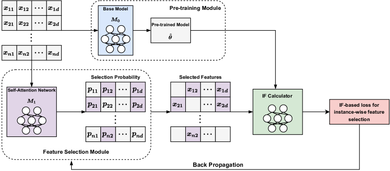
Figure 1. The overall architecture of the proposed DIWIFT, where the core components are a feature selection model with a self-attention network, and an IF calculator for calculating the value of the corresponding influence function.

4.1. Theoretical Analysis

According to the definition of feature-level IF in Eq.(2), we can approximate the loss change of $z_{j}\sim Q(\bm{x},y)$ if $z_{i}\sim P(\bm{x},y)$ is perturbed by $\delta_{i}\in\mathbb{R}^{d}$,

(3) $$l(z_{j},\hat{\theta}_{\delta_{i}})-l(z_{j},\hat{\theta})\approx\phi(z_{i},z_{j})\delta_{i}.$$

This process can be extended to the whole validation set as follows,

(4) $$\sum_{j=1}^{m}l(z_{j},\hat{\theta}_{\delta_{i}})-\sum_{j=1}^{m}l(z_{j},\hat{\theta})\approx[\sum_{j=1}^{m}\phi(z_{i},z_{j})]\delta_{i},$$

where $m$ is the size of the validation set. Obviously, the best perturbation should minimize the validation loss $\sum_{j=1}^{m}l(z_{j},\hat{\theta}_{\delta_{i}})$. We then have the optimization problem about $\delta_{i}$,

(5) $$\delta_{i}^{*}=\arg\min_{\delta_{i}}\sum_{j=1}^{m}l(z_{j},\hat{\theta}_{\delta_{i}})=\arg\min_{\delta_{i}}\phi_{i}\delta_{i},$$

where $\phi_{i}=\sum_{j=1}^{m}\phi(z_{i},z_{j})\in\mathbb{R}^{1\times d}$ indicates the influence of instance $z_{i}$ over the whole validation set.

Let the $k$-th dimension of $\phi_{i}$, $\delta_{i}$ and $\bm{x}_{i}$ be denoted as $\phi_{ik}$, $\delta_{ik}$ and $\bm{x}_{ik}$, respectively. For the adversarial training problems where the feature values are dense and continuous, such as image data, the optimal $\delta_{i}^{*}$ is in the direction of $\phi_{i}^{T}$ (Koh and Liang, 2017). However, for the problem of feature selection in tabular data, the range of values for $\delta_{ik}$ is $\{0,-\bm{x}_{ik}\}$, where $\delta_{ik}=0$ means $\bm{x}_{ik}$ remains unchanged, and $\delta_{ik}=-\bm{x}_{ik}$ means $\bm{x}_{ik}$ is removed. Moreover, in tabular data, the one-hot encoded sparse feature value $\bm{x}_{ik}$ is in $\{0,1\}$, and the normalized dense feature value $\bm{x}_{ik}$ is in $[0,1]$. Thus, $\delta_{ik}\leq 0$ always holds, and the solution of Eq.(5) is,

(6) $$\delta_{ik}^{*}=\begin{cases}0&\text{if }\phi_{ik}<0,\\ -\bm{x}_{ik}&\text{if }\phi_{ik}\geq 0.\end{cases}$$

The results in Eq.(6) is intuitive because $\phi_{ik}\geq 0$ means the presence of $\bm{x}_{ik}$ will increase the validation loss, for which we should indeed remove this feature. Recall the feature selection matrix $S$ defined in Section 3, we can see that, if a feature $k$ in $z_{i}$ is selected, i.e., $S_{ik}=1$, then both conditions should be satisfied, i.e., $\bm{x}_{ik}>0$ and $\delta_{ik}=0$. We then get the theoretically optimal $S^{*}_{ik}$,

(7) $$S_{ik}^{*}=\mathds{1}(\phi_{ik}\bm{x}_{ik}<0),$$

where $\mathds{1}(\cdot)$ is a 0-1 indicator function.

This means that by minimizing the validation loss of the model trained after instance-wise feature selection, we can obtain the optimal instance-wise feature selection strategy in Eq.(7) with the help of the influence function. Note that the influence function allows the model to trade off between the training and validation distributions (Yu et al., 2020), and the resulting instance-wise feature selection method is expected to perform robustly in the scenarios where a distribution shift exist. Next, we describe the proposed DIWIFT method in detail, which is a new instance-wise feature selection method based on the influence function, and verify its robustness in the experiments. To the best of our knowledge, most existing works on feature selection have not considered the variability of influential features across different scenarios.

4.2. Discovering Instance-wise Influential Features in Tabular Data

In this section, based on the theoretical insights in Section 4.1, we propose a novel method for discovering instance-wise influential features in tabular data, or DIWIFT for short.

4.2.1. Architecture

The overall framework of our DIWIFT is illustrated in Figure 1. As shown in Figure 1, the core steps of our DIWIFT include: 1) a pre-training module aims to train on a base model $M_{0}$ based on the original tabular data, i.e., without feature selection, in order to obtain a set of pre-trained model parameters $\hat{\theta}$. These model parameters are required in the subsequent steps to calculate the value of the influence function as shown in Eq.(2). Although $\hat{\theta}$ is theoretically the parameter of the optimal empirical risk minimizer, we may not be able to obtain an accurate $\hat{\theta}$ in practice because the deep learning model is non-convex. To this end, we will perform a sensitivity analysis about our DIWIFT with some pre-trained models of varying performance in our experiments; 2) a feature selection module with a self-attention network $M_{1}$ receives the original tabular data and outputs the corresponding instance-wise feature selection probabilities; 3) after feature selection is performed on each instance according to the selection probability, these new instances and the pre-trained model $\hat{\theta}$ are fed into the IF calculator to calculate the value of the corresponding influence function; and 4) the calculated value of the influence function is used to calculate the IF-based loss designed in Eq.(14) for instance-wise feature selection, and then the feature selection model $M_{1}$ is updated by means of back propagation.

Note that since the self-attention mechanism has shown its effectiveness and flexibility in previous related works (Zhou et al., 2018; Škrlj et al., 2020; Qin et al., 2020), we employ a self-attention network in the feature selection module as an example, to capture the importance of instance-wise features driven by the influence function. However, the self-attention mechanism is not a necessary structure, and in fact, any neural network layer that can generate a mask matrix of the same dimension as the input can be used as a feature selection model. After obtaining the feature selection model $M_{1}$, we need to refine the base model $M_{0}$ based on the original instance to obtain the final prediction model, where the original instance will first undergo a feature selection process through $M_{1}$. Similarly, in the prediction stage, each instance will go through a process of instance-wise feature selection through $M_{1}$, and then get the predicted label that is fed into the final prediction model. Next, we will give a detailed introduction to the important modules in our DIWIFT.

4.2.2. Feature selection module

As described in Section 4.2.1, we use a self-attention network in the feature selection module to effectively model the selection probability, since a self-attention (Vaswani et al., 2017) has been proven to be a useful module that can capture important features in instances (Zhou et al., 2018; Škrlj et al., 2020; Qin et al., 2020). We first use a multi-head attention on an instance to get its embedding representation. Specifically, we have,

(8) $$Q=K=V=\left(\mathbf{e}_{1};\mathbf{e}_{2};\dots;\mathbf{e}_{i};\dots;\mathbf{e}_{d}\right),$$

where $\mathbf{e}_{i}$ denotes the embedding representation of the $i$-th feature, $Q=K=V\in R^{d\times K_{d}}$ and $K_{d}$ is the dimension of the output embedding. Then, the computation of self-attention can be expressed as,

(9) $$Attention(Q,K,V)=softmax(\frac{QK^{T}}{\sqrt{K_{d}}})V.$$

Further, the multi-head self-attention can be calculated as follows,

(10) $$E =Multihead(Q,K,V)$$

$$=Concatenate(head_{1},head_{2},\dots,head_{h})W^{O},$$

where $h$ denotes the number of self-attention networks, $head_{i}$ = $Attention(Q_{i},K_{i},V_{i})$ and $W^{O}\in R^{hK_{d}\times K_{d}}$ is a parameter matrix. After obtaining the embedding representation $E$ of an instance, we feed it into a multi-layer perceptron (MLP) with a $ReLU$ activation function to obtain the corresponding output for each instance,

(11) $$f(x,\omega)=MLP(E),$$

where $f(\bm{x},\omega):\mathbb{R}^{d}\rightarrow\mathbb{R}^{d}$ denotes the mapping from an input feature vector to a corresponding output, i.e., a feature selection model based on a self-attention network, and $\omega$ denotes the parameters of this model.

We design the probability of selecting each corresponding feature as

(12) $$p(\bm{x},\omega)=\sigma(f(\bm{x},\omega)/\tau),$$

where $p(\bm{x},\omega)\in\mathbb{R}^{d}$, $\sigma(\cdot)$ is the sigmoid function, $\tau\in\mathbb{R}^{+}$ is the alterable temperature parameter. We propose to relate the temperature control coefficient to the number of training iterations, i.e., $\tau=\max(\tau_{min},1-(1-\tau_{min})t/t_{max})$, where $\tau_{min}$ is a sufficiently small minimum temperature parameter (e.g., 0.001 used in the experiments), $t$ is the current number of iterations, and $t_{max}$ is the maximum number of iterations. Obviously, as the number of training iterations increases, $\tau$ will gradually decrease to a small enough value, and this will ensure that the selection probability of each feature is close to 0 or 1 to obtain the discrete feature selection mask. For ease of understanding, we present a structure of the feature selection model in Figure 2.

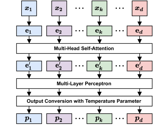
Figure 2. The structure of a feature selection model with a self-attention network, where the embedding representation of each instance is $E=\left(\mathbf{e}^{\prime}_{1},\mathbf{e}^{\prime}_{2},\dots,\mathbf{e}^{\prime}_{d}\right)$.

4.2.3. IF calculator

In this subsection, we introduce the influence function to guide the training of a feature selection model and further improve the accuracy and robustness of instance-wise feature selection for tabular data. According to the definition of IF in Eq.(2), we can find that the calculation of IF is usually complicated. Therefore, we need to solve the problem of how to calculate IF efficiently. Let $p_{i}$ and $p_{j}$ be the selection probabilities of the features in $z_{i}$ and $z_{j}$, respectively, where $p_{i}=\left[p_{i1},p_{i2},\dots,p_{id}\right]$ and $p_{j}=\left[p_{j1},p_{j2},\dots,p_{jd}\right]$. After obtaining the pre-trained model parameters $\hat{\theta}$ and reweighting the features using $p_{i}$ and $p_{j}$, the influence of $z_{i}$ on the entire validation set is,

(13) $$\phi_{i}(p(\bm{x},\omega))=-[\sum_{j=1}^{m}\nabla_{\theta}l(p_{j}\odot\bm{x}_{j},y_{j},\hat{\theta})]^{\top}$$

$$H_{\hat{\theta}}(p)^{-1}\nabla_{\bm{x}}\nabla_{\theta}l(p_{i}\odot\bm{x}_{i},y_{i},\hat{\theta}),$$

where $\odot$ is the element-wise product and $H_{\hat{\theta}}(p)=\frac{1}{n}\sum_{i=1}^{n}\nabla^{2}_{\theta}l(p_{i}\odot\bm{x}_{i},y_{i},\hat{\theta})$. The influence function $\phi_{i}(p(\bm{x},\omega))$ can be calculated in three steps: 1) we compute the inverse Hessian-vector-product (HVP) $[\nabla_{\theta}\sum_{j=1}^{m}l(p_{j}\odot\bm{x}_{j},y_{j},\hat{\theta})]^{\top}H_{\hat{\theta}}(p)^{-1}$ and set the result as a constant vector independent of the derivative of $\bm{x}$; 2) for each training instance, we multiply the constant vector with $\nabla_{\theta}l(p_{i}\odot\bm{x}_{i},y_{i},\hat{\theta})$; and 3) finally, we take the derivative with respect to $\bm{x}$. The most difficult step is computing HVP, and we use a stochastic estimation method from previous studies (Koh and Liang, 2017) to efficiently handle high-dimensional and large-scale tabular data. In the stochastic estimation method, let $H_{u}^{-1}=\sum_{v=0}^{u}(I-H)^{v}$ be the first $u$ terms in the Taylor expansion of $H^{-1}$, where $H$ is an arbitrary Hessian matrix and $I$ is the identity matrix. We then have $H_{u}^{-1}=I+(I-H)H_{u-1}^{-1}$, $H_{u}^{-1}\rightarrow H^{-1}$ when $u\rightarrow\infty$. The key step is that in each iteration, we can sample some instances to compute an unbiased estimator of $H$. Therefore, we can get the following calculation process for HVP: 1) uniformly sample some instances from the training set and calculate the Hession matrix $\tilde{H}$; 2) define $H_{0}^{-1}\mu=\mu$, where $\mu=[\nabla_{\theta}\sum_{j=1}^{m}l(p_{j}\odot\bm{x}_{j},y_{j},\hat{\theta})]$ in the feature selection; and 3) recursively compute $H_{u}^{-1}\mu=\mu+(I-\tilde{H})H_{u-1}^{-1}\mu$. Note that the computational complexity of the original IF is $O(np^{2}+p^{3})$, where $p$ is the dimension of model parameters, and the complexity of stochastic estimation used is $O(np+rtp)$, where $r$ is the number of samples sampled, and $t$ is the number of sampling executions. We can find that DIWIFT is of good scalability by comparing these two complexities. The complete process of calculating $\phi_{i}(p(\bm{x},\omega))$ is shown in Algorithm 1 of Appendix A.

4.2.4. IF-based loss for instance-wise feature selection

The final optimization objective of our DIWIFT is to minimize the sum of $\phi_{ik}$ of the selected $\bm{x}_{ik}$:

(14) $$\hat{\omega}=\arg\min_{\omega}\sum_{i=1}^{n}\phi_{i}(p(\bm{x},\omega))[p(\bm{x}_{i},\omega)\odot\mathds{1}(\bm{x}_{i})],$$

where $\mathds{1}(\bm{x}_{i})\in\mathbb{R}^{d}$ transfers the $k$-th dimension of $\bm{x}_{i}$ to 1 if $\bm{x}_{ik}>0$, and otherwise to 0. We can see that $p(\bm{x}_{i},\omega)\odot\mathds{1}(\bm{x}_{i})$ means feature $\bm{x}_{ik}$ has no probability to be selected if $\bm{x}_{ik}=0$. The complete training process of our DIWIFT is shown in Algorithm 2 of Appendix A.

5. Empirical Evaluations

In this section, we conduct experiments with the aim of answering the following five key questions.

• Q1: How does our DIWIFT perform compared to the baselines?

• Q2: How well does our DIWIFT identify the instance-wise influential features?

• Q3: How do different modules of our DIWIFT contribute to its performance?

• Q4: How does our DIWIFT perform in presence of distribution shift?

• Q5: How robust is our DIWIFT to fluctuations in a pre-trained model?

5.1. Experimental Setup

5.1.1. Datasets.

To comprehensively evaluate the performance of our DIWIFT, we consider both some synthetic datasets and real-world datasets in our experiments. We first generate three synthetic datasets following the approach adopted in previous related works (Chen et al., 2018; Yoon et al., 2018). Specifically, the input features are generated from an 11-dimensional Gaussian distribution, where there is no correlation between the features, i.e., $\bm{x}\sim\mathcal{N}(\bm{0},\mathbf{I})$. The $k$-th feature is denoted as $\bm{x}^{k}$. The label $y$ is generated from a Bernoulli random variable with $\mathbb{P}(y=1|\bm{x})=\frac{1}{1+logit(\bm{x})}$, where $logit(\bm{x})$ can vary to create three different synthetic datasets:

• Syn1: exp$\left(\bm{x}^{1}\bm{x}^{2}\right)$.

• Syn2: $-10\times\sin 2\bm{x}^{7}+2\left|\bm{x}^{8}\right|+\bm{x}^{9}+\mathrm{exp}(-\bm{x}^{10})$.

In the above two datasets, the generation of labels $y$ depends on the same set of features for each instance. To compare the ability of different methods to discover instance-wise influence features, by setting $\bm{x}^{11}$ as a switch feature, we create a new synthetic dataset, where different instances have different influence features.

• Syn3: If $\bm{x}^{11}<0$, $logit(\bm{x})$ follows Syn1; otherwise, $logit(\bm{x})$ follows Syn2.

In addition, we employ four datasets, including Coat (Schnabel et al., 2016), Adult (Kohavi et al., 1996), Bank, and Credit (Dal Pozzolo et al., 2014), that are widely adopted in previous works focusing on modeling tabular data (Kim et al., 2021; Luo et al., 2019). The statistics of all the datasets are summarized in Table 3. In subsequent experiments, we divide all instances of each dataset into a training set, a validation set and a test set, where each part corresponds to a ratio of $3:1:1$.

Table 3. Statistics of three synthetic datasets and four real-world datasets.

Datasets	#Features	#Instances
Syn1	11	30k
Syn2	11	30k
Syn3	11	30k
Coat	47	11k
Adult	137	49k
Bank	55	45k
Credit	30	284k

5.1.2. Baselines

We choose the most representative methods from the two routes as the baselines, including two global feature selection methods, i.e., Lasso (Fonti and Belitser, 2017) and Tree (Geurts et al., 2006), and four instance-wise feature selection methods, i.e., L2X (Chen et al., 2018), CL2X (Panda et al., 2021), INVASE (Yoon et al., 2018) and TabNet (Arik and Pfister, 2021).

• Lasso (Fonti and Belitser, 2017): it is a widely used global feature selection method via adding $L_{1}$ regularization to the loss of a linear model.

• Tree (Geurts et al., 2006): it is a global feature selection method via an extremely randomized trees classifier.

• L2X (Chen et al., 2018): it is an instance-wise feature selection method that can discover a fixed number of influential features for each instance through mutual information. It is the first method to implement instance-wise feature selection and interpretation.

• CL2X (Panda et al., 2021): it is a causal extension of L2X that also discovers a fixed number of influential features for each instance via conditional mutual information.

• INVASE (Yoon et al., 2018): it is an instance-wise feature selection method that can discover an adaptive number of influential features for each instance by minimizing the Kullback-Leibler divergence between the full conditional distribution and a conditional distribution that includes only the selected set of features. It is an important baseline because it best matches the problem we focus on solving in this paper.

• TabNet (Arik and Pfister, 2021): it is an instance-based feature selection method that uses sequential attention to select the features that need to be inferred at each decision step. Furthermore, it proposes a novel high-performance and interpretable deep learning architecture for tabular data.

5.1.3. Evaluation Metrics.

We apply the Area Under the ROC Curve (AUC) as the evaluation metric, which is commonly adopted in previous studies of tabular data (Xie et al., 2021; Arik and Pfister, 2021). Specifically, the AUC in binary classification task is calculated by,

$$AUC=\frac{\sum_{z_{p}\in z^{+},z_{q}\in z^{-}}\mathds{1}(g(z_{p})>g(z_{q}))}{|z^{+}||z^{-}|},$$

where $z^{+}$ is the set of positive instances, $z^{-}$ is the set of negative instances, $|z^{+}|$ and $|z^{-}|$ are their sizes; $z_{p}$ is a positive instance, $z_{q}$ is a negative instance; $g(\cdot)$ is a classifier. Note that if the predicted scores of all positive samples are higher than the predicted scores of negative samples, the model will reach AUC$=1$ (perfect separation of positive/negative samples), i.e., the upper bound of AUC is 1, and the bigger the better.

5.1.4. Implementation Details

For all the methods, a three-layer MLP is adopted as a base model. For the search range, $L_{2}$ regularization parameter is in $[1e^{-6},1]$, learning rate is in $[1e^{-5},1e-1]$, hidden layer size is in $\left\{50,100,150,200\right\}$, and batch size is in $\left\{64,128,256,512,1024,2048\right\}$. A special $L_{1}$ parameter with LASSO is in $[1e^{-5},1e^{-1}]$, and Tree needs to set the number of trees from 3 to 30. For L2X and CL2X , we set the number of features selected in each instance in the range of $[2,d]$. For our DIWIFT, temperature parameter is in $[1e^{-3},1]$. Regarding the error analysis, we calculate the standard deviation of the AUC metric on the test set through 10 random experiments. The standard deviation is calculated as follows:

(15) $$deviation=\sqrt{\frac{1}{N}\sum_{i=1}^{N}(s_{i}-\frac{1}{N}\sum_{j=1}^{N}s_{j})^{2}},$$

where $N$ denotes the number of random trials and $s_{i}$ means the AUC score at the $i$-th experiment.

Table 4. Results on all the datasets, where the best results are marked in bold and the second best results are underlined. AUC is the evaluation metric.

Method	Syn1	Syn2	Syn3	Coat	Adult	Bank	Credit
No-selection	0.5934±0.0001	0.8268±0.0004	0.7001±0.0001	0.6598±0.0172	0.8908±0.0043	0.9175±0.0004	0.8857±0.0003
Lasso	0.6868±0.0012	0.8651±0.0006	0.7199±0.0002	0.6482±0.0009	0.8972±0.0045	0.8887±0.0004	0.9460±0.0005
Tree	0.6786±0.0002	0.8840±0.0003	0.7241±0.0001	0.6538±0.0176	0.8966±0.0041	0.8854±0.0006	0.9251±0.0221
L2X	0.6218±0.0083	0.8758±0.0206	0.6874±0.0018	0.6631±0.0093	0.8985±0.0035	0.9019±0.0026	0.9258±0.0090
CL2X	0.6262±0.0431	0.8278±0.0003	0.6941±0.0015	0.6627±0.0011	0.9046±0.0044	0.9160±0.0001	0.9122±0.0049
INVASE	0.6442±0.0011	0.8842±0.0002	0.7765±0.0009	0.6693±0.0115	0.8996±0.0036	0.9179±0.0835	0.9107±0.0370
TabNet	0.6732±0.0006	0.9068±0.0001	0.7819±0.0002	0.6694±0.0010	0.9074±0.0001	0.9182±0.0022	0.9308±0.0347
DIWIFT	0.6900±0.0019	0.9013±0.0055	0.7851±0.0014	0.6736±0.0034	0.9231±0.0031	0.9231±0.0055	0.9495±0.0019

5.2. RQ1: Performance Comparison

To verify the effectiveness of our DIWIFT, we conduct the comparative experiments with all the baselines. The detailed results are shown in Table 4. The method named “No-selection” is a baseline that uses all the features rather than some selected features. From Table 4, we have the following observations: 1) the comparison results between the baselines for instance-wise feature selection and global feature selection are inconsistent across different datasets. TabNet is the best baseline overall. This may be because L2X and CL2X can only discover a fixed number of influential features per instance, and INVALSE is not specifically designed for tabular data. However, TabNet does not have these limitations. 2) our DIWIFT outperforms all the baselines in most cases, except slightly weaker than TabNet on the Syn2 dataset. In particular, our DIWIFT significantly outperforms TabNet on the syn3 dataset with varying numbers of influential features per instance, as well as on all the four real-world datasets.

5.3. RQ2: Visual Verification of DIWIFT

Does our DIWIFT effectively discover instance-wise influential features? To answer this question, we randomly sample 10 instances from the Syn3 dataset, of which 5 instances follow Syn1 and the remaining instances follow Syn2, since the ground truth of the instance-wise influential features is given in the Syn3 dataset. These 10 instances are then fed into the feature selection module of our DIWIFT to get the feature selection result corresponding to each instance. The results are shown in Figure 3, where each row represents an instance, each column represents a feature, the blue squares represent the ground truth of influential features in each instance, and the stars represent the feature selection results of our DIWIFT. We can find that our DIWIFT can identify the most influential instance-wise features and removing the most non-influential features. This again verifies the validity of our DIWIFT.

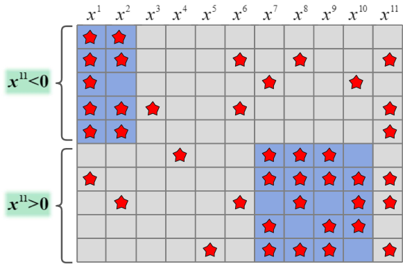
Figure 3. An example of the feature selection results our DIWIFT has on the syn3 dataset, where each row represents an instance, each column represents a feature, the blue squares represent the ground truth of the influential features in each instance, and the stars represent the selected features by our DIWIFT. Note that with $x^{11}$ as a switch feature, the first five instances follow Syn1, and the last five instances follow Syn2.

5.4. RQ3: Ablation Study

As described in Section 4.2, the feature selection module and the IF calculator are the core modules of our DIWIFT. To analyze their respective roles, we conduct ablation studies on our DIWIFT using the four real-world datasets. The results are shown in Figure 4, where “w/o influence” means that only the IF calculator is removed (i.e., a self-attention module trained using a traditional loss function is retained), and “No-selection” means that both the feature selection module and the IF calculator are removed. We can see that removing any module will hurt the performance. In addition, “w/o influence” is weaker than our DIWIFT, but is still better than “No-selection”, which also shows the importance of feature selection for modeling tabular data.

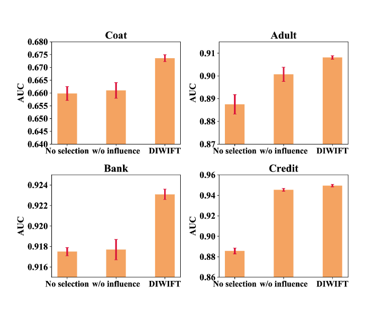
Figure 4. Ablation studies on four real-world datasets.

5.5. RQ4&RQ5: In-Depth Analysis of DIWIFT

As described in Section 4.1, most existing works on feature selection has not considered the variability of influential features across different scenarios. Conversely, our DIWIFT can benefit from the influence function to achieve a trade-off between training and validation distributions, i.e., it is relatively more robust. To evaluate the robustness of all the methods under a distribution shift scenario, we choose the Coat dataset in our experiments. The Coat dataset contains the sets collected from two sources: one is a biased data collected through the normal user interactions on an online web-shop platform, and the other is an unbiased data collected through a randomized experiment, in which all items that a user can see are randomly assigned by the system. Clearly, there is a distribution shift between these two sets. We re-partition Coat, where the set of biased data is used as a training set, and the set of unbiased data is randomly divided into a validation set and a test set with equal size. We then re-execute and evaluate all the methods using the same hyperparameter search range, and show the results in Figure 5. Comparing with the Coat column in Table 4, we can find that all the baselines have a significant drop in performance, which is even weaker than “No-selection”. This shows that the existing feature selection methods are susceptible to distribution shift. Conversely, our DIWIFT is more robust and has a distinct advantage in different scenarios.

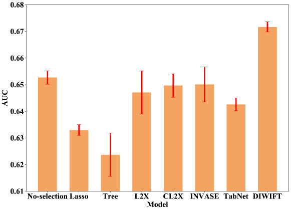
Figure 5. Robustness analysis on Coat.

Finally, we perform a sensitivity analysis of our DIWIFT with the pre-trained models of different performance. As described in Section 4.2.1, the influence function calculator is an important module of our DIWIFT, and its computation requires the parameters of a pretrained model $\hat{\theta}$. Since the computed value of the influence function will be used to guide the training of a feature selection module, which is another core module of our DIWIFT, it is necessary to analyze the sensitivity of our DIWIFT on pretrained models with different performance. Next, we examine this sensitivity of our DIWIFT by conducting a preliminary experiment on Coat. When obtaining the results of our DIWIFT on Coat as shown in Table 4, the optimal number of training iterations for the pre-trained model is 18. Therefore, we choose the base model when the number of training iterations is 8, 10, 12, 14, and 16 as the pre-trained model, respectively. We then retrain our DIWIFT and evaluate its performance. The results are shown in Figure 6. We can see that our DIWIFT is relatively insensitive to the pre-trained model. This observation is important for deploying our DIWIFT in a real-world scenario, as it shows that we can use the same pre-trained model for a period of time, which will effectively save training time.

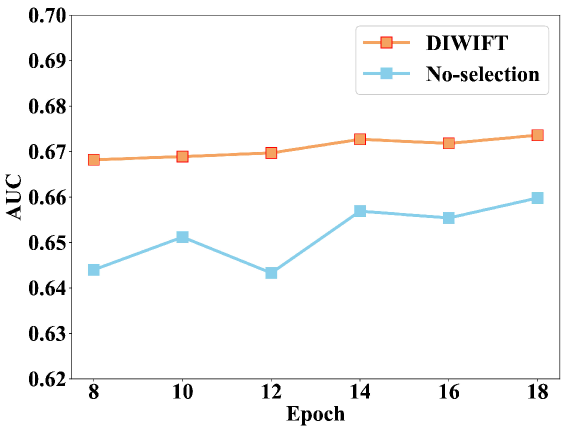
Figure 6. Sensitivity analysis of our DIWIFT with different pre-trained models on Coat.

6. Conclusions

In this paper, we propose a new perspective based on the influence function for instance-wise feature selection and give some corresponding theoretical insights. We then propose a new method for discovering instance-wise influential features in tabular data (DIWIFT), where a feature selection module with a self-attention network is used to compute the selection probabilities of all features from each instance, and an influence function calculator is used to calculate the corresponding influence and guide the feature selection module through a back propagation. We conduct extensive experiments on some synthetic and real-world datasets, where the results validate the effectiveness and robustness of our DIWIFT.

Appendix A Appendix

Algorithm 1 Calculating the influence function $\phi_{i}(p(\bm{x},\omega))$

0:  The training set after feature reweighting $\{p_{i}\odot\bm{x}_{i},y_{i}\}_{i=1}^{n}$, validation set $\{\{p_{j}\odot\bm{x}_{j},y_{j}\}_{j=1}^{m}$, pre-trained base network $\hat{\theta}$.

1:  Calculate the gradient of the validation loss, i.e., $\mu=[\nabla_{\theta}\sum_{j=1}^{m}l(p_{j}\odot\bm{x}_{j},y_{j},\hat{\theta})]$.

2:  Initialize $H_{0}^{-1}\mu=\mu$.

3:  repeat to get HVP

4:  Uniformly sample some instances from the training set to calculate the estimated Hession matrix $\tilde{H}$.

5:  Calculate $H_{u}^{-1}\mu=\mu+(I-\tilde{H})H_{u-1}^{-1}\mu$.

6:  until convergence

7:  Refer to $h$ as the converged HVP, which is the estimation of $H_{\hat{\theta}}(p)^{-1}[\nabla_{\theta}\sum_{j=1}^{m}l(p_{j}\odot\bm{x}_{j},y_{j},\hat{\theta})]$.

8:  Calculate $\nabla_{\theta}l(p_{i}\odot\bm{x}_{i},y_{i},\hat{\theta})$.

9:  Calculate the gradient of $h^{T}\nabla_{\theta}l(p_{i}\odot\bm{x}_{i},y_{i},\hat{\theta})\in\mathbb{R}$ over $\bm{x}$.

Algorithm 2 Discovering Instance-wise Influential Features in Tabular Data (DIWIFT)

0:  The training set $\{z_{i}\}_{i=1}^{n}$, validation set $\{z_{j}\}_{j=1}^{m}$.

1:  Train a base model to get $\hat{\theta}$.

2:  Initialize all parameters of a feature selection model with a self-attention network.

3:  repeat

4:  Fed instances into feature selection model to get probability $p_{i}$ and $p_{j}$ using Eq.(12).

5:  Calculate the influence function in Eq.(13) using the stochastic estimation method.

6:  Calculate the loss in Eq.(14).

7:  Do back-propagation to update the parameters of the feature selection model.

8:  until convergence

- (1)
- Arik and Pfister (2021) Sercan Ö Arik and Tomas Pfister. 2021. TabNet: Attentive interpretable tabular learning. In Proceedings of the 35th AAAI Conference on Artificial Intelligence. 6679–6687.
- Borisov et al. (2021) Vadim Borisov, Tobias Leemann, Kathrin Seßler, Johannes Haug, Martin Pawelczyk, and Gjergji Kasneci. 2021. Deep neural networks and tabular data: A survey. arXiv preprint arXiv:2110.01889 (2021).
- Chen et al. (2022) Jintai Chen, Kuanlun Liao, Yao Wan, Danny Z Chen, and Jian Wu. 2022. DANets: Deep abstract networks for tabular data classification and regression. In Proceedings of the 36th AAAI Conference on Artificial Intelligence. 3930–3938.
- Chen et al. (2018) Jianbo Chen, Le Song, Martin Wainwright, and Michael Jordan. 2018. Learning to explain: An information-theoretic perspective on model interpretation. In Proceedings of the 35th International Conference on Machine Learning. 883–892.
- Dal Pozzolo et al. (2014) Andrea Dal Pozzolo, Olivier Caelen, Yann-Ael Le Borgne, Serge Waterschoot, and Gianluca Bontempi. 2014. Learned lessons in credit card fraud detection from a practitioner perspective. Expert Systems with Applications 41, 10 (2014), 4915–4928.
- Doleschal et al. (2018) Johannes Doleschal, Nico Höllerich, Wim Martens, and Frank Neven. 2018. CHISEL: Sculpting tabular and non-tabular data on the web. In Companion Proceedings of The Web Conference 2018. 139–142.
- Fonti and Belitser (2017) Valeria Fonti and Eduard Belitser. 2017. Feature selection using lasso. VU Amsterdam Research Paper in Business Analytics 30 (2017), 1–25.
- Geurts et al. (2006) Pierre Geurts, Damien Ernst, and Louis Wehenkel. 2006. Extremely randomized trees. Machine learning 63, 1 (2006), 3–42.
- Guyon and Elisseeff (2003) Isabelle Guyon and André Elisseeff. 2003. An introduction to variable and feature selection. Journal of Machine Learning Research 3 (2003), 1157–1182.
- Huber (2011) Peter J Huber. 2011. Robust statistics. In International Encyclopedia of Statistical Science. Springer, 1248–1251.
- Katzir et al. (2020) Liran Katzir, Gal Elidan, and Ran El-Yaniv. 2020. Net-DNF: Effective deep modeling of tabular data. In Proceedings of the 9th International Conference on Learning Representations.
- Kim et al. (2021) Jayoung Kim, Jinsung Jeon, Jaehoon Lee, Jihyeon Hyeong, and Noseong Park. 2021. OCT-GAN: Neural ode-based conditional tabular gans. In Proceedings of The Web Conference 2021. 1506–1515.
- Koh and Liang (2017) Pang Wei Koh and Percy Liang. 2017. Understanding black-box predictions via influence functions. In Proceedings of the 34th International Conference on Machine Learning. 1885–1894.
- Kohavi et al. (1996) Ron Kohavi et al. 1996. Scaling up the accuracy of naive-Bayes classifiers: A decision-tree hybrid. In Proceedings of the 2nd International Conference on Knowledge Discovery and Data Mining. 202–207.
- Liu et al. (2020) Zhaocheng Liu, Qiang Liu, Haoli Zhang, and Yuntian Chen. 2020. DNN2LR: Interpretation-inspired feature crossing for real-world tabular data. arXiv preprint arXiv:2008.09775 (2020).
- Luo et al. (2019) Yuanfei Luo, Mengshuo Wang, Hao Zhou, Quanming Yao, Wei-Wei Tu, Yuqiang Chen, Wenyuan Dai, and Qiang Yang. 2019. AutoCross: Automatic feature crossing for tabular data in real-world applications. In Proceedings of the 25th ACM SIGKDD International Conference on Knowledge Discovery and Data Mining. 1936–1945.
- Luo et al. (2020) Yuanfei Luo, Hao Zhou, Wei-Wei Tu, Yuqiang Chen, Wenyuan Dai, and Qiang Yang. 2020. Network on network for tabular data classification in real-world applications. In Proceedings of the 43rd International ACM SIGIR Conference on Research and Development in Information Retrieval. 2317–2326.
- Lyu et al. (2023a) Fuyuan Lyu, Xing Tang, Dugang Liu, Liang Chen, Xiuqiang He, and Xue Liu. 2023a. Optimizing feature set for click-through rate prediction. arXiv preprint arXiv:2301.10909 (2023).
- Lyu et al. (2023b) Fuyuan Lyu, Xing Tang, Dugang Liu, Haolun Wu, Chen Ma, Xiuqiang He, and Xue Liu. 2023b. Feature representation learning for click-through rate prediction: A review and new perspectives. arXiv preprint arXiv:2302.02241 (2023).
- Panda et al. (2021) Pranoy Panda, Sai Srinivas Kancheti, and Vineeth N Balasubramanian. 2021. Instance-wise causal feature selection for model interpretation. In Proceedings of the 2021 Conference on Computer Vision and Pattern Recognition. 1756–1759.
- Pang et al. (2021) Guansong Pang, Chunhua Shen, Longbing Cao, and Anton Van Den Hengel. 2021. Deep learning for anomaly detection: A review. ACM Computing Surveys 54, 2 (2021), 1–38.
- Qin et al. (2020) Jiarui Qin, Weinan Zhang, Xin Wu, Jiarui Jin, Yuchen Fang, and Yong Yu. 2020. User behavior retrieval for click-through rate prediction. In Proceedings of the 43rd International ACM SIGIR Conference on Research and Development in Information Retrieval. 2347–2356.
- Ren et al. (2018) Mengye Ren, Wenyuan Zeng, Bin Yang, and Raquel Urtasun. 2018. Learning to reweight examples for robust deep learning. In Proceedings of the 35th International Conference on Machine Learning. 4334–4343.
- Schnabel et al. (2016) Tobias Schnabel, Adith Swaminathan, Ashudeep Singh, Navin Chandak, and Thorsten Joachims. 2016. Recommendations as treatments: Debiasing learning and evaluation. In Proceedings of the 33rd International Conference on Machine Learning. 1670–1679.
- Škrlj et al. (2020) Blaž Škrlj, Sašo Džeroski, Nada Lavrač, and Matej Petkovič. 2020. Feature importance estimation with self-attention networks. In Proceedings of the 24th European Conference on Artificial Intelligence. 1491–1498.
- Sliwinski et al. (2019) Jakub Sliwinski, Martin Strobel, and Yair Zick. 2019. Axiomatic characterization of data-driven influence measures for classification. In Proceedings of the 33rd AAAI Conference on Artificial Intelligence. 718–725.
- Ucar et al. (2021) Talip Ucar, Ehsan Hajiramezanali, and Lindsay Edwards. 2021. SubTab: Subsetting features of tabular data for self-supervised representation learning. In Proceedings of the 35th Conference on Neural Information Processing Systems. 18853–18865.
- Vaswani et al. (2017) Ashish Vaswani, Noam Shazeer, Niki Parmar, Jakob Uszkoreit, Llion Jones, Aidan N Gomez, Łukasz Kaiser, and Illia Polosukhin. 2017. Attention is all you need. In Proceedings of the 31st International Conference on Neural Information Processing Systems. 6000–6010.
- Wang et al. (2018) Tianyang Wang, Jun Huan, and Bo Li. 2018. Data dropout: Optimizing training data for convolutional neural networks. In Proceedings of the 30th International Conference on Tools with Artificial Intelligence. 39–46.
- Wang et al. (2020) Zifeng Wang, Hong Zhu, Zhenhua Dong, Xiuqiang He, and Shao-Lun Huang. 2020. Less is better: Unweighted data subsampling via influence function. In Proceedings of the 34th AAAI Conference on Artificial Intelligence. 6340–6347.
- Xie et al. (2021) Yuexiang Xie, Zhen Wang, Yaliang Li, Bolin Ding, Nezihe Merve Gürel, Ce Zhang, Minlie Huang, Wei Lin, and Jingren Zhou. 2021. FIVES: Feature interaction via edge search for large-scale tabular data. In Proceedings of the 27th ACM SIGKDD International Conference on Knowledge Discovery and Data Mining. 3795–3805.
- Yoon et al. (2018) Jinsung Yoon, James Jordon, and Mihaela van der Schaar. 2018. INVASE: Instance-wise variable selection using neural networks. In Proceedings of the 6th International Conference on Learning Representations.
- Yu et al. (2020) Jiangxing Yu, Hong Zhu, Chih-Yao Chang, Xinhua Feng, Bowen Yuan, Xiuqiang He, and Zhenhua Dong. 2020. Influence function for unbiased recommendation. In Proceedings of the 43rd International ACM SIGIR Conference on Research and Development in Information Retrieval. 1929–1932.
- Zhang et al. (2019) Shuai Zhang, Lina Yao, Aixin Sun, and Yi Tay. 2019. Deep learning based recommender system: A survey and new perspectives. ACM Computing Surveys 52, 1 (2019), 1–38.
- Zhou et al. (2018) Guorui Zhou, Xiaoqiang Zhu, Chenru Song, Ying Fan, Han Zhu, Xiao Ma, Yanghui Yan, Junqi Jin, Han Li, and Kun Gai. 2018. Deep interest network for click-through rate prediction. In Proceedings of the 24th ACM SIGKDD International Conference on Knowledge Discovery and Data Mining. 1059–1068.