Forecasting the detection capabilities of third–generation gravitational–wave detectors using GWFAST

Abstract

We introduce GWFAST, a novel Fisher–matrix code for gravitational–wave studies, tuned toward third–generation gravitational–wave detectors such as Einstein Telescope (ET) and Cosmic Explorer (CE). We use it to perform a comprehensive study of the capabilities of ET alone, and of a network made by ET and two CE detectors, as well as to provide forecasts for the forthcoming O4 run of the LVK collaboration. We consider binary neutron stars, binary black holes and neutron star–black hole binaries, and compute basic metrics such as the distribution of signal–to–noise ratio (SNR), the accuracy in the reconstruction of various parameters (including distance, sky localization, masses, spins and, for neutron stars, tidal deformabilities), and the redshift distribution of the detections for different thresholds in SNR and different levels of accuracy in localization and distance measurement. We examine the expected distribution and properties of ‘golden events’, with especially large values of the SNR. We also pay special attention to the dependence of the results on astrophysical uncertainties and on various technical details (such as choice of waveforms, or the threshold in SNR), and we compare with other Fisher codes in the literature. In the companion paper Iacovelli et al. (2022) we discuss the technical aspects of the code. Together with this paper, we publicly release the code GWFAST  , and the library WF4Py   implementing state–of–the–art gravitational–wave waveforms in pure Python.

tablenum SIXtablenum

ET-0141A-22

1 Introduction

The discoveries made in the last few years by the LIGO and Virgo gravitational wave (GW) detectors have opened a new window on the Universe. After the first historic detection of the GWs from a binary black hole (BBH) coalescence in September 2015 (Abbott et al., 2016), and the first detection in 2017 of a binary neutron star (BNS) coalescence and the identification and follow–up of its electromagnetic counterpart (Abbott et al., 2017a, b), which opened the field of multi–messenger astronomy, GW observations have become a routine, with detections made on a weekly basis. After three observing runs (O1–O3), the current catalog of GW detections contains about 90 events, mostly BBHs, but include also two BNSs and two neutron star–black hole (NSBH) binaries (Abbott et al., 2021a, b). These discoveries are already starting to have a remarkable impact on astrophysics, cosmology and fundamental physics including, e.g., studies of population properties of compact binary systems (Abbott et al., 2021c), tests of General Relativity (Abbott et al., 2021d), the determination of the speed of GWs to one part in $10^{15}$ (Abbott et al., 2017b), first constraints on the expansion history of the Universe using GWs (Abbott et al., 2021e), or constraints on the neutron star equation of state (Hernandez Vivanco et al., 2019).

Currently LIGO and Virgo, now joined by KAGRA and forming the LVK collaboration, are further improving their sensitivity and preparing for their fourth observational run, O4, scheduled for 2023, and eventually for the O5 run, currently scheduled for 2026–2028. However, the community has long been preparing the jump toward ‘third–generation’ (3G) detectors, Einstein Telescope (ET) in Europe (Punturo et al., 2010; Hild et al., 2011) and Cosmic Explorer (CE) in the US (Reitze et al., 2019; Evans et al., 2021). Thanks to an increase by one order of magnitude in sensitivity and a significant enlargement of the bandwidth toward both low and high frequencies, these detectors will have an extraordinary potential for discoveries. In particular, for coalescing binaries, they will allow us to make a huge jump in the distances reached, in the number of detections, in the accuracy of signal reconstructions, and in the range of masses that can be explored, providing data that have the potential of triggering revolutions in fundamental physics, in cosmology and in astrophysics. Building on many previous works, the science case for 3G detectors is being systematically investigated (see Maggiore et al. (2020); Kalogera et al. (2021) and references therein). The activity around 3G detectors recently received a significant boost from the inclusion of ET in the ESFRI Roadmap, the roadmap of large European scientific infrastructures, resulting in an acceleration of activities around ET and, very recently, the ET Collaboration has formally been created at the XII ET Symposium. On the US side, activity around Cosmic Explorer has started more recently, and has led to the Cosmic Explorer Horizon Study document (Evans et al., 2021).

A crucial aspect, in order to assess the scientific potential of 3G detectors, is the development of codes that allow us to forecast the performance of these detectors, in terms of some rather general “metrics”, such as the distribution of signal–to–noise ratio (SNR) for coalescing binaries, and the accuracy in the reconstruction of their parameters; in particular, distance, sky localization, masses, spins and, for neutron stars, quantities (such as the tidal deformability) that are sensitive to their inner structure. It is also very important to understand the reach in redshift of these detectors and how the distribution in SNR and parameter reconstruction depends on redshift. The reference tool for this kind of investigations is an approach based on the Fisher matrix. Despite some of its well–known limitations, that we will review in Sect. 2, this is at the moment the only computationally feasible way of performing parameter estimation on large populations, such as the $10^{4}-10^{5}$ BBHs and BNSs per year that, as we will discuss below, 3G detectors are expected to detect. This tool also allows us to compare the performance of different configurations of a given detector, and of different detector networks, which is necessary in order to take informed decisions on individual detector designs and on optimal network configurations.

For this reason, a number of parameter estimation codes tuned to 3G detectors have been developed recently, in particular GWBENCH (Borhanian, 2021) and GWFISH (Harms et al., 2022) [see also Chan et al. (2018); Grimm & Harms (2020); Nitz & Dal Canton (2021); Li et al. (2022); Pieroni et al. (2022)]. In this paper we present a novel parameter estimation code, GWFAST, also meant mainly for application to 3G detectors. The existence of several different parameter estimation codes is a welcome, and in fact necessary, feature; these codes can contribute to taking decisions on detectors which are meant to dominate the scientific landscape for decades (and require the huge financial and human resources typical of Big Science), so they must be extremely reliable and have undergone cross–checks between different groups, that developed different codes independently. In this spirit, we have undergone a process of cross–checking between GWBENCH, GWFISH and GWFAST, which are, arguably, the most complete and advanced codes currently available, finding broad consistency. Each of these codes has different technical implementations. We discuss the technical aspects of our code, together with reliability and performance tests, in the companion paper Iacovelli et al. (2022), while here we briefly summarize them in Sect. 3.3. One relevant aspect is that the problem of computing Fisher matrices for a large catalog of independent events is clearly parallel. Parallelization techniques can be used, but one limitation of current Python–based implementations is that they still usually compute the SNRs and Fisher matrices serially on each node/CPU. In our implementation, we are able to ‘vectorize’ the evaluation of the Fisher matrices even on a single CPU (on top of the use of parallel computing), resulting in a gain in computational speed, which is at the origin of the name GWFAST. This is also due to the implementation of the waveforms in Python, which motivated the development and release of the library WF4Py. Furthermore, this allows us to make use of automatic differentiation to compute derivatives, which is a technique alternative to finite differences leading to faster and more robust evaluations. Note that GWFAST also supports an interface with the LIGO Algorithm Library, LAL (LIGO Scientific Collaboration, 2018), which allows the use of all waveforms available in this library.

In this paper we discuss the results obtained for BBHs, BNSs and NSBHs with our code, and we compare them, in particular, with those reported for BBHs and BNSs in Borhanian & Sathyaprakash (2022) (using GWBENCH), and for BNSs in Ronchini et al. (2022) (which uses GWFISH). The comparison also needs to take care of different assumptions on astrophysical populations, that reflect our current uncertainties, as well as of different technical choices (waveforms, thresholds on SNR, detector network configurations, etc.). Our results will then contribute to giving an overall picture of the capabilities of 3G detectors. Compared in particular to Borhanian & Sathyaprakash (2022), our work is more focused on ET. To avoid a proliferation of plots, and of lines in each plot, in this work we will only report the results for two 3G configurations: ET alone, and a network of ET together with two CE detectors (ET+2CE), and we will compare them with the expectations for the forthcoming LVK–O4 run. Studying ET alone allows us to assess the strength of the ET Science Case, independently of decisions that will be taken by different funding agencies on CE. On the other hand, combining ET with two CE detectors allows us to examine the full strength of a 3G detector network. Our code, however, can be used to study a large variety of networks.

The paper is organized as follows. In Sect. 2 we recall the Fisher matrix formalism, as well as its limitations. In Sect. 3 we discuss the modelization of the GW signal. In particular, since BNSs can stay in the bandwidth of 3G detectors for as long as hours or a day, it is important to include the effect of the Earth’s rotation on the signal, which can be exploited to improve the sky localization of the source. In Sect. 4 we discuss the assumptions that we make on the astrophysical populations of BBHs, BNSs and NSBHs, and we present the detectors that we will study, computing their horizon (and the distance at which $50\%$ of the events are detected) for different type of sources. Sect. 5 contains the bulk of our results for parameter estimation of BBHs, BNSs and NSBHs. Further results are included in the Appendices, including, in App. B, a comparison with the results presented in Borhanian & Sathyaprakash (2022) and in Ronchini et al. (2022).

2 Formalism for parameter estimation

2.1 Fisher Information Matrix

In this section we recall the basic formalism and interpretation of the use of the Fisher matrix formalism in GW parameter estimation. We refer to Cutler & Flanagan (1994); Vallisneri (2008); Rodriguez et al. (2013) for comprehensive treatments. We assume that the time–domain signal in a GW detector can be written as the superposition of an expected signal $h_{0}$ and stationary, Gaussian noise $n$ with zero mean:

$$s(t)=h_{0}(t)+n(t)\;.$$ (1)

The statistical properties of the noise are encoded in the one–sided power spectral density, defined by

$$\langle\tilde{n}^{*}(f)\,\tilde{n}(f^{\prime})\rangle=\frac{1}{2}\delta(f-f^{\prime})S_{n}(f)\;,$$ (2)

where the tilde denotes a temporal Fourier transform. This determines an inner product for any two time–domain signals $a(t)$, $b(t)$:

$$\left(a\,|\,b\right)=4\Re{\int_{0}^{\infty}\differential{f}\,\frac{\tilde{a}^{*}(f)\,\tilde{b}(f)}{S_{n}(f)}}\;.$$ (3)

Under the assumption of stationarity and Gaussianity, from Eq. (2) we have that the variance of a Fourier mode with frequency $f$ is $S_{n}(f)/2$, so the probability that the noise has a given distribution $n_{0}$ can be written in terms of Eq. (3) as $p(n_{0})\propto\exp{-\left(n_{0}\,|\,n_{0}\right)/2}.$ Together with Eq. (1), this results in the following likelihood for a data realisation $s$ conditioned on the waveform parameters ${\bf\it\theta}$:

$$\mathcal{L}(s\;|\;{\bf\it\theta})\propto\exp{-\left(s-h({\bf\it\theta})\,|\,s-h({\bf\it\theta})\right)/2}\;.$$ (4)

Note that ${\bf\it\theta}$ refers to the parameters of the template waveform model, which may be different from the ones of the actual signal $h_{0}$, that we denote by ${\bf\it\theta}_{0}$. Using Eq. (3) we can also express the signal–to–noise ratio (SNR) of the true signal as

$$\text{SNR}=\left(h_{0}\,|\,h_{0}\right)^{\nicefrac{{1}}{{2}}}\;.$$ (5)

The Fisher Information Matrix (FIM) for the likelihood in Eq. (4) is defined as:

$$\Gamma_{ij}\equiv-\evaluated*{\langle\partial_{i}\partial_{j}\log\mathcal{L}(s\,|\,{\bf\it\theta})\rangle_{n}}_{{\bf\it\theta}={\bf\it\theta}_{0}}=\left(h_{i}\,|\,h_{j}\right)\;,$$ (6)

where $h_{i}\equiv\partial_{i}h$, and the notation $\langle\,\dots\rangle_{n}$ denotes an average over noise realizations with fixed parameters. The last equality is a consequence of the property $\langle\left(a\,|\,n\right)\left(n\,|\,b\right)\rangle_{n}=\left(a\,|\,b\right)$ that follows from Eq. (2). Intuitively, near a maximum of the likelihood, the latter is approximated by a multivariate Gaussian with covariance $\Gamma_{ij}^{-1}$. To understand the correct interpretation of this statement it is useful to consider an expansion of the template signal around the waveform with true parameters’ values ${\bf\it\theta}_{0}$ as

$$h({\bf\it\theta})=h_{0}+h_{i}\,\delta\theta^{i}+\dots\qquad\;,$$ (7)

where $\delta\theta^{i}\equiv\theta^{i}-\theta_{0}^{i}$. This approximation, where only first derivatives of the signal are included, is known as the linearized signal approximation (LSA). The LSA likelihood is obtained by inserting Eq. (7) in Eq. (4):

$$\mathcal{L}(s\,|\,{\bf\it\theta})\propto\exp[-\frac{1}{2}\left(n\,|\,n\right)+\delta\theta^{i}\left(n\,|\,h_{i}\right)-\frac{1}{2}\delta\theta^{i}\delta\theta^{j}\left(h_{i}\,|\,h_{j}\right)\Big{]}\;.$$ (8)

It can be shown that the LSA is equivalent to the limit of large SNR (Vallisneri, 2008). Two interpretations of the meaning of the FIM appearing in Eq. (8) are possible:

• From a frequentist point of view, one can compute the maximum likelihood (ML) estimator $\hat{{\bf\it\delta\theta}}$ and its covariance over noise realizations at fixed parameters, which yields

  $$\hat{\delta\theta}^{i} ={\left(h_{i}\,|\,h_{j}\right)}^{-1}\left(n\,|\,h_{j}\right)\,,$$ (9)

  $$\langle\hat{\delta\theta}^{i}\hat{\delta\theta}^{j}\rangle_{n} =\left(h_{i}\,|\,h_{j}\right)^{-1}\,.$$

  This shows that the inverse of the FIM is equal to the covariance of the frequentist maximum–likelihood estimator in the LSA/large SNR limit and for Gaussian noise.

• From a Bayesian perspective one can compute the mean and variance of the posterior probability $p({\bf\it\theta}\,|\,s)\propto p({\bf\it\theta})\mathcal{L}({\bf\it\theta}\,|\,s)$. Using a flat prior $p({\bf\it\theta})\propto\text{const.}$, we obtain

  $$\langle{\delta\theta}^{i}\rangle =\frac{\int\differential{\bf\it\theta}\,{\delta\theta}^{i}\,p({\bf\it\theta}\,|\,s)}{\int\differential{\bf\it\theta}\,p({\bf\it\theta}\,|\,s)}={\left(h_{i}\,|\,h_{j}\right)}^{-1}\left(n\,|\,h_{j}\right)\,,$$ (10)

  $$\langle{\delta\theta}^{i}{\delta\theta}^{j}\rangle =\langle\big{(}{\delta\theta}^{i}-\langle{\delta\theta}^{i}\rangle\big{)}\big{(}{\delta\theta}^{j}-\langle{\delta\theta}^{j}\rangle\big{)}\rangle=\left(h_{i}\,|\,h_{j}\right)^{-1}\,.$$

  In the above equations, $\langle\,\dots\rangle$ denotes an average over parameter realizations at fixed data. Hence, the inverse of the FIM is also equal to the covariance of the Bayesian posterior probability distribution of the true parameters ${\bf\it\theta}_{0}$ for a given experiment with data $s$, assuming: a flat prior, the LSA/large SNR limit and Gaussian noise.

The Bayesian point of view is the most useful to compare to results of an actual parameter estimation as well as to incorporate the effects of priors on the source parameters. In this case, one can explicitly re–write the LSA likelihood (omitting factors that do not depend on ${\bf\it\delta\theta}$) as

$$\mathcal{L}(s\,|\,{\bf\it\theta})\propto\exp\left[-\frac{1}{2}\left(h_{i}\,|\,h_{j}\right)\big{(}\delta\theta^{i}-\langle{\delta\theta}^{i}\rangle\big{)}\big{(}\delta\theta^{j}-\langle{\delta\theta}^{j}\rangle\big{)}\right]\,.$$ (11)

On the other hand, in absence of real data, as is the case when forecasting parameter estimation capabilities of future experiments, it makes sense also to consider the frequentist approach which makes statements about ensembles of possible data realizations (Cutler & Flanagan, 1994).

Finally, another important interpretation of the FIM concerns the Cramer–Rao bound: the inverse FIM gives the lower bound for the covariance of any unbiased estimator of the true parameters ${\bf\it\theta}_{0}$ under different noise realization (hence, it is a frequentist error estimate). However, its interpretation is subtle (Vallisneri, 2008) and this bound does not translate in a bound on the variance of the Bayesian posterior (Rodriguez et al., 2013).

2.2 Singularities

The most relevant issues when computing the FIM are the accurate computation of the derivatives and the presence of singularities, which can result in instability of the numerical inversion. The computational aspects as implemented in GWFAST are described in Sect. 3.3, while here we discuss the interpretation of singular or ill–conditioned matrices.

If the FIM is exactly singular, the likelihood has one or more directions in parameter space along which it is exactly constant, corresponding to null eigenvalues. If the LSA approximation was exact, one could conclude that one or more combination of parameters are impossible to constrain and discard them. In particular, one can discard the combination of parameters corresponding to the null singular values of a singular–value decomposition. However, this is true only in the LSA, as higher–order contributions may cure the singularity, and using this approach in the FIM does not necessarily lead to realistic forecasts of the parameter estimation performance, since only truly degenerate combinations should be discarded.

A more common situation to face in practice is the case where the matrix is not exactly singular but ill conditioned, i.e. the inverse of the condition number (defined as the ratio of the largest to the smallest eigenvalues) is comparable or smaller than machine precision. This can lead to large amplifications of inversion errors, resulting in a covariance that may be inaccurate even at the 100% level. Condition numbers might be improved by numerical techniques (see Sect. 3.3 for the implementation in GWFAST), but the physical interpretation is that the directions in parameter space corresponding to small eigenvalues need large variations of the parameters to produce relevant changes in the waveform (at least comparable to the noise level). Hence, the LSA might no longer be sufficient to accurately describe the likelihood over all the range of interest (Vallisneri, 2008), even if the SNR at the true parameters’ values is high enough. We will discuss this point in Sect. 3.3. One can resort to some regularization of the singularities, for example truncating the singular values of the singular–value decomposition to the minimum allowed numerical precision; however this has not a direct link to actual generalizations of the FIM that might cure the singularity, such as the inclusion of higher order terms (or of priors, see Sect. 2.3). In general, when using the FIM to forecast parameter estimation, one must be aware that the bad conditioning of the matrix is pointing to some possible breakdown of the LSA on the likelihood surface irrespective of the specific regularization technique used.

In this work we prefer not to resort to regularization of the singular values nor to discard combinations of parameters corresponding to small eigenvalues. The reason is that this might lead to underestimating the errors on the waveform parameters that are most affected by degeneracies, unless careful checks and comparisons with other methods are performed.

One possible alternative approach corresponds to discarding all the matrices with condition number larger than the inverse machine precision. This is the most conservative option, which might on the other hand lead to discarding many events for which a sensible inversion of the Fisher matrix could still be obtained. A somewhat intermediate possibility is to discard all the events for which the inversion error of the FIM is larger than a given threshold. In this work [as, e.g., in Berti et al. (2005), see their App. B], we adopt the latter strategy and quantify the inversion error as

$$\epsilon={||\Gamma\cdot\Gamma^{-1}-\mathbb{1}||}_{\rm max}=\max_{ij}|(\Gamma\cdot\Gamma^{-1}-\mathbb{1})_{ij}|\;.$$ (12)

The chosen threshold for this work is $\epsilon_{\rm max}=$5\text{\times}{10}^{-2}$$. In App. C we detail the choice of this value and compare the results with other methods to obtain forecasts on the uncertainty, including a direct sampling from the likelihood in Eq. (11) which does not rely on the inversion of the Fisher matrix. In App. B we compare to other choices in the literature and discuss the impact of different approaches on the population of sources studied in this paper.

In a Bayesian context, the use of priors can cure singularities and is the most realistic way to proceed, as priors are actually used in parameter estimation. We discuss the role of priors in the next section, while their effect is also studied in App. Cfv.

2.3 Role of priors

In a Bayesian parameter estimation problem, prior distributions are expected to have a role whenever their information content is more restrictive than the one in the likelihood, typically either because the prior changes significantly in the region of non–vanishing likelihood or because hard boundaries are present. If the LSA is valid, the presence of priors can play an important role in curing possible singularities of the FIM. In practice, the FIM formalism allows to treat in a simple way only the case of a Gaussian prior $p(\mathbf{\theta})\propto\exp{-P_{ij}\delta\theta^{i}\delta\theta^{j}}$, in which case adding the prior amounts to substitute $\left(h_{i}\,|\,h_{j}\right)\mapsto\left(h_{i}\,|\,h_{j}\right)+P_{ij}$ in Eq. (10)–(11), i.e. to add the prior matrix to the FIM.

In a GW parameter estimation problem, we have to deal with the fact that some parameters might require priors that are far from Gaussian, in particular to incorporate information on the physical range of some of them, such as the symmetric mass ratio $\eta$ (which is constrained to be in the range $[0;\,0.25]$), the luminosity distance $d_{L}$ (constrained to be positive), and the angles. In Markov chain Monte Carlo (MCMC) analyses, priors on the angles might not be used if not for increasing speed, since the full likelihood carries information on the periodicity of these variables. In contrast, the Fisher formalism does not have any information about the periodicity of the likelihood with respect to some parameters, hence the use of a prior can be a more realistic choice. For angular variables, a crude but simple approximation can be the use of a Gaussian prior of width $2\pi$. The situation is more complicated for other parameters, in particular $\eta$ and $d_{L}$. When using a FIM analysis to forecast overall trends in future experiments rather than concentrating on single events, one can check that the majority of the events have a predicted $1\sigma$ contour that does not exceed the physical boundary. For more realistic estimates, an exact prior can be included by explicitly drawing samples from the likelihood in Eq. (11), using rejection sampling to account for the prior, and estimating the posterior covariance from the remaining samples. We show the effect of adopting this procedure, and compare it to different inversion methods, in App. C.

2.4 Limits of applicability

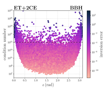
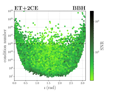
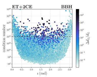
Figure 1: Scatter plot of the condition numbers of the Fisher matrices as a function of the system inclination angle, computed for BBH events detected at a network consisting of ET+2CE, using the IMRPhenomHM waveform model. In the left panel we report on the color bar the inversion errors associated with the events and in the central panel the SNRs and in the right panel the relative errors on the luminosity distance. The horizontal dashed line shows the inverse machine precision limit, of ${10}^{15}$.

We have seen that the applicability of the FIM relies on the LSA/high SNR limit. From the discussion in Sect. 2.2, however, it is clear that such an approximation should hold within all the likelihood region of interest – for example, the 1$\sigma$ or 2$\sigma$ contours. For this to be the case, not only the SNR at the true values should be high, but of particular relevance is the problem of conditioning: a high condition number might signal a breakdown of the LSA in the region of interest (Finn, 1992; Vallisneri, 2008).

One instructive example concerns the inclination angle of the source with respect to the observer, $\iota$. The amplitudes of the two GW polarisations depend differently on this parameter and their joint measurement would allow disentangling $\iota$ from the distance to the source. However, it is for nearly face–on binaries ($\iota\sim 0$) that the signal is louder, but in this case the two polarisations are nearly equal (Nissanke et al., 2010; Schutz, 2011; Usman et al., 2019), which leads to a strong degeneracy of the inclination angle with the distance to the source. Thus, an event observed face–on will be louder than the same system observed in an inclined configuration, but its FIM will be ill–conditioned. In the limit of exactly face–on systems, $\iota=0$, and ignoring the presence of higher modes in the GW signal, the FIM will even be exactly degenerate, since the first derivative of the signal with respect to $\iota$ vanishes exactly in this limit. We refer to Fig. 1 for an illustration based on the population studied in this work. This shows that, for events with nearly face–on configuration, we can be in the situation where the SNR is large but the FIM is ill–conditioned (Cutler & Flanagan, 1994).

In practise, assessing the validity of the LSA on all the likelihood surface without explicitly calculating higher–order corrections or resorting to explicit Monte Carlo analyses is a subtle problem. Vallisneri (2008) proposed a “maximum mismatch criterion” to determine the validity of the LSA, which consists in sampling the $1\sigma$ likelihood surface, compute the difference between the waveforms on this surface and at the true value, $\Delta h=h({\bf\it\theta}_{1\sigma})-h_{0}$ and computing the ratio $r$ of the LSA likelihood to the full likelihood, which can be shown to be

$$|\log(r)|=\frac{1}{2}\,\left(\theta^{i}h_{i}-\Delta h\,|\theta^{j}h_{j}-\Delta h\,h_{j}\right)\;.$$ (13)

Then, a signal can be considered linear if some threshold is satisfied by this mismatch, for example by requiring that $|\log(r)|<0.1$ for $90\%$ of the points on the $1\sigma$ likelihood surface (Vallisneri, 2008; Rodriguez et al., 2013). This is an internal consistency criterion rather than a proof of validity. However, explicit comparison with MCMC showed that, while this is indeed a sufficient condition for the LSA, many systems showing good agreement between the FIM and a full MCMC analysis failed this test (Rodriguez et al., 2013). In summary, there seems not to be a conclusive, flexible and computationally cheap test to assess the validity of the FIM over all the surface of interest. In this work we apply the threshold on the inversion error of the FIM described in Sect. 2.2 and App. C. However, one must be aware of such limitations of the FIM approach. We believe these issues to be a further motivation for the development and comparison of different implementations of the FIM technique, in order to assess the robustness of the predictions to different choices.

3 Modeling the gravitational–wave signal

The response of a detector to a GW signal emitted by a coalescing binary system is given by a linear combination of the two polarisations $(h_{+},h_{\times})$, obtained by their projection on the detector arms by suitable “antenna pattern functions” $(F_{+},F_{\times})$ that depend on the source position and polarisation angle, as well as the location, orientation and shape of the detector, which we denote collectively by ${\bf\it\lambda}$. In full generality, we denote the parameters of the waveform by ${\bf\it\theta}=\{{\cal M}_{c},\eta,d_{L},\theta,\phi,\iota,\psi,t_{c},\Phi_{c},\chi_{1,x},\chi_{2,x},\chi_{1,y},\chi_{2,y},\chi_{1,z},\chi_{2,z},\Lambda_{1},\Lambda_{2}\}$ [see e.g. Maggiore (2007)], where ${\cal M}_{c}$ denotes the detector–frame chirp mass, $\eta$ the symmetric mass ratio, $d_{L}$ the luminosity distance to the source, $\theta$ and $\phi$ are the sky position coordinates, defined as $\theta=\pi/2-\delta$ and $\phi=\alpha$ (with $\alpha$ and $\delta$ right ascension and declination, respectively), $\iota$ the inclination angle of the binary with respect to the line of sight, $\psi$ the polarisation angle, $t_{c}$ the time of coalescence, $\Phi_{c}$ the phase at coalescence, $\chi_{i,c}$ the dimensionless spin of the object $i=\{1,2\}$ along the axis $c=\{x,y,z\}$ and $\Lambda_{i}$ the dimensionless tidal deformability of the object $i$ (which is present only for systems containing a NS). Instead of $\Lambda_{1},\Lambda_{2}$, we will actually use (Wade et al., 2014)

$$\tilde{\Lambda} =\dfrac{8}{13}\left[(1+7\eta-31\eta^{2})(\Lambda_{1}+\Lambda_{2})+\sqrt{1-4\eta}(1+9\eta-11\eta^{2})(\Lambda_{1}-\Lambda_{2})\right]\,,$$ (14a)

$$\delta\tilde{\Lambda} =\dfrac{1}{2}\left[\sqrt{1-4\eta}\left(1-\dfrac{13272}{1319}\eta+\dfrac{8944}{1319}\eta^{2}\right)(\Lambda_{1}+\Lambda_{2})+\left(1-\dfrac{15910}{1319}\eta+\dfrac{32850}{1319}\eta^{2}+\dfrac{3380}{1319}\eta^{3}\right)(\Lambda_{1}-\Lambda_{2})\right]\,,$$ (14b)

which have the advantage that $\tilde{\Lambda}$ is the combination that enters the inspiral waveform at 5 PN, while $\delta\tilde{\Lambda}$ first enters at 6 PN.

In the time domain, the signal of the quadrupole mode is given by

$$h(t,{\bf\it\theta},{\bf\it\lambda})=A_{+}(t,{\bf\it\theta})F_{+}(t,{\bf\it\theta},{\bf\it\lambda})\cos{\Phi(t,{\bf\it\theta})}+A_{\times}(t,{\bf\it\theta})F_{\times}(t,{\bf\it\theta},{\bf\it\lambda})\sin{\Phi(t,{\bf\it\theta})}\,.$$ (15)

The amplitudes $A_{+,\times}$ and the phase $\Phi$ are obtained from a waveform model. We describe the models used in Sect. 3.1. In particular, in this work and in GWFAST we work in the frequency domain. In this case, when computing the full signal in Eq. (15), an important point is that the low–frequency sensitivity of 3G detectors, and in particular of ET, makes it possible to observe the inspiral phase of low–mass events, such as BNSs, for several hours to possibly one day. In those cases the pattern functions evolve in time during the detection due to the change in the relative position of the source and the detector. Since we work in frequency rather than time domain, it is important to correctly account for this time evolution when Fourier transforming the signal. We describe this in detail in Sect. 3.2.

3.1 Waveform models

We adopt Fourier domain full inspiral–merger–ringdown models, tuned on Numerical Relativity (NR) simulations. Our code can be adapted to a large variety of waveforms. As reference waveforms, for BBH, BNS and NSBH systems, we will use, respectively:

IMRPhenomHM

(London et al., 2018; Kalaghatgi et al., 2020) this is a recent model, tuned for BBH systems (in quasi–circular orbits) with non–precessing spins, which takes into account the quadrupole of the signal and the sub–dominant modes $(l,m)=(2,1),\ (3,2),\ (3,3),\ (4,3),\ {\rm and}\ (4,4)$. The contribution of these higher modes is of fundamental importance for parameter estimation, since they can break the degeneracy between the luminosity distance and inclination angle. In fact, each mode depends on a different combination of sines and cosines of the inclination angle $\iota$, through the spin–weighted spherical harmonics ${}_{-2}Y^{lm}$ (Goldberg et al., 1967), while the fundamental mode (2,2), only depends on the cosine, leading to a degeneracy with $d_{L}$;

IMRPhenomD_NRTidalv2

(Dietrich et al., 2019) this model is an extension of IMRPhenomD (Husa et al., 2016; Khan et al., 2016a), which also accounts for tidal effects in BNS systems. In fact, the two neutron stars in a coalescing binary, differently from black holes, will deform when getting closer to each other, and this leaves clear signatures on the waveform, which have to be accurately modelled and tuned to specific NR simulations;

IMRPhenomNSBH

(Pannarale et al., 2015; Dietrich et al., 2019), this model can describe the signals coming from the merger of a NS and a BH, which have very distinctive features. In particular, the mass ratios of these systems can be much higher than that of BNSs and BBHs, so this model is tuned up to $q\sim 100$, and it also accounts for tidal effects, since the NS will deform getting closer to the BH. Moreover, this model is built and tuned to account for the fact that, when it is close enough to the BH, the NS can either plunge into it or get disrupted forming an accretion torus (Lattimer & Schramm, 1976), two scenarios that result in very different features on the waveforms.

We will then perform a comparison between the results obtained using different waveform models. Note that, in addition to the above waveform models, GWFAST includes Python implementations of the models TaylorF2_RestrictedPN and IMRPhenomD, as well as a wrapper to all waveforms contained in the LIGO Algorithm Library, LAL (note, however, that when using the latter, which are implemented in C, it is no longer possible to exploit Python vectorization).

3.2 Detector response and effect of Earth’s rotation

In this work and in GWFAST we use the expression of the ‘pattern functions’ which takes into account the rotation of the Earth given in Jaranowski et al. (1998). We collectively denote the parameters characterizing the detector by ${\bf\it\lambda}=\{\lambda,\ \varphi,\ \gamma,\ \zeta\}$, where $\zeta$ is the angle between the detector’s arms (e.g. $90\text{\,}\mathrm{\SIUnitSymbolDegree}$ for an L–shaped detector), $\lambda$ and $\varphi$ are the detector’s latitude and longitude, respectively, and $\gamma$ is the angle formed by the arms bisector and East. We then have for the pattern functions:

$$F_{+}(t;\theta,\phi,\psi,{\bf\it\lambda}) =\sin{\zeta}\,\big{[}a(t;\theta,\phi,{\bf\it\lambda})\cos{2\psi}+b(t;\theta,\phi,{\bf\it\lambda})\sin{2\psi}\big{]}\,,$$ (16)

$$F_{\times}(t;\theta,\phi,\psi,{\bf\it\lambda}) =\sin{\zeta}\,\big{[}b(t;\theta,\phi,{\bf\it\lambda})\cos{2\psi}-a(t;\theta,\phi,{\bf\it\lambda})\sin{2\psi}\big{]}\,,$$

with (omitting from now on the explicit dependence on the parameters)

$$a(t) =\dfrac{1}{16}\sin{2\gamma}(3-\cos{2\lambda})(3+\cos{2\theta})\cos{[2(\phi-\varphi-2\pi f_{\oplus}t)]}-\dfrac{1}{4}\cos{2\gamma}\sin{\lambda}(3+\cos{2\theta})\sin{[2(\phi-\varphi-2\pi f_{\oplus}t)]}$$ (17)

$$\quad\,+\dfrac{1}{4}\sin{2\gamma}\sin{2\lambda}\sin{2\theta}\cos{(\phi-\varphi-2\pi f_{\oplus}t)}-\dfrac{1}{2}\cos{2\gamma}\cos{\lambda}\sin{2\theta}\sin{(\phi-\varphi-2\pi f_{\oplus}t)}$$

$$\quad\,+\dfrac{3}{4}\sin{2\gamma}\cos^{2}{\lambda}\sin^{2}{\theta}\,,$$

$$b(t) =\cos{2\gamma}\sin{\lambda}\cos{\theta}\cos{[2(\phi-\varphi-2\pi f_{\oplus}t)]}+\dfrac{1}{4}\sin{2\gamma}(3-\cos{2\lambda})\cos{\theta}\sin{[2(\phi-\varphi-2\pi f_{\oplus}t)]}$$

$$\quad\,+\cos{2\gamma}\cos{\lambda}\sin{\theta}\cos{(\phi-\varphi-2\pi f_{\oplus}t)}+\dfrac{1}{2}\sin{2\gamma}\sin{2\lambda}\sin{\theta}\sin{(\phi-\varphi-2\pi f_{\oplus}t)}\,,$$

where $f_{\oplus}\simeq$1\text{\,}{\mathrm{day}}^{-1}$$ is the Earth’s rotational frequency.

The effect of the Earth’s rotation on the signal consists of an amplitude modulation, due to the variation of the pattern functions with time as in Eq. (16), a phase modulation arising for the same reason, due to the fact that the pattern functions relative to the two polarisations evolve differently in time, and a Doppler contribution to the phase due to the relative motion between the source and the detector (Cutler, 1998; Cornish & Larson, 2003). In time domain, the Doppler contribution can be conveniently expressed as a time–dependent shift of the time variable [see, e.g. Sect. 7.6.2 of Maggiore (2007) and Wen & Chen (2010)]. We work with signals in frequency domain. To compute the Fourier transform one can adopt the Stationary Phase Approximation, that applies if the change in the amplitude during a cycle is much slower than the corresponding change in the phase. This is the case for each of the two terms in the sum in Eq. (15), so, neglecting for the moment the time shift due to the Doppler effect, we get

$$\tilde{h}_{+,\times}(f) =\int A_{+,\times}(t)F_{+,\times}(t)\cos{\Phi(t)}\,e^{2\pi ift}\differential{t}$$ (18)

$$\simeq\dfrac{1}{2}A_{+,\times}(t^{\ast})F_{+,\times}(t^{\ast})\left(\dfrac{2\pi}{\ddot{\Phi}(t^{\ast})}\right)^{\nicefrac{{1}}{{2}}}\exp{i\left[2\pi ft^{\ast}\,-\,\Phi(t^{\ast})-\dfrac{\pi}{4}\right]}\,,$$

where the stationary point $t^{\ast}(f)$ is determined by the condition $2\pi f=\dot{\Phi}(t^{\ast})$. To lowest order in the post–Newtonian (PN) expansion, this gives

$$t^{\ast}(f)=t_{c}-\dfrac{5}{256}\left(\dfrac{G{\cal M}_{c}}{c^{3}}\right)^{-\nicefrac{{5}}{{3}}}(\pi f)^{-\nicefrac{{8}}{{3}}}\times\left[1+\order{(\pi fGM_{\rm tot}/c^{3})^{\nicefrac{{2}}{{3}}}}\right]\,,$$ (19)

where $t_{c}$ is the time of coalescence and $M_{\rm tot}$ the total mass of the system. Note, however, that in our analysis we compute the time to coalescence at 3.5 PN order, as in Buonanno et al. (2009b), Eq. (3.8b). The amplitude modulation is reflected in the fact that the Fourier transformed signal contains the expressions of $F_{+}$ and $F_{\times}$ evaluated at the stationary point $t^{\ast}(f)$, according to Eq. (18) (see also Zhao & Wen (2018)). An illustration of this effect is given in Fig. 2, for a BNS signal analogous to GW170817.

We next consider the Doppler effect due to the rotation of the Earth around its axis. Its contribution to the calculation of $t^{\ast}(f)$ and to the amplitude of the Fourier transform on the right–hand side of Eq. (18) is totally negligible, since the frequency scale $1\,{\rm day}^{-1}$ is very small compared to the frequencies relevant for ground–based detectors, so we only need to consider its effect in the phase. This is encoded in the time dependence of the time delay corresponding to the travel time of the signal from the origin of the reference frame, i.e. the center of the Earth, to the detector. This time delay in time domain results in a phase shift in Fourier domain, known as location phase factor, given by

$$\phi_{L}=2\pi f\Delta t_{L}=-2\pi f\dfrac{R_{\oplus}}{c}\hat{{\bf\it s}}(\theta,\phi)\dotproduct\hat{{\bf\it d}}(\lambda,\varphi,t^{\ast}(f))\,,$$ (20)

where $R_{\oplus}\simeq$6371\text{\,}\mathrm{km}$$ is the Earth’s radius, $\hat{{\bf\it s}}(\theta,\phi)$ and $\hat{{\bf\it d}}(\lambda,\varphi)$ are the unit vectors pointing to the source and the detector, respectively, with the second one being evaluated at the stationary point $t^{\ast}(f)$ when including Earth’s rotation, i.e.

$$\hat{{\bf\it s}}(\theta,\phi) =\Big{(}\sin{\theta}\cos{\phi},\ \sin{\theta}\sin{\phi},\ \cos{\theta}\Big{)}\,,$$ (21)

$$\hat{{\bf\it d}}(\lambda,\varphi,t^{\ast}(f)) =\Big{(}\cos{\lambda}\cos{(\varphi+2\pi f_{\oplus}t^{\ast})},\ \cos{\lambda}\sin{(\varphi+2\pi f_{\oplus}t^{\ast})},\ \sin{\lambda}\Big{)}\,.$$

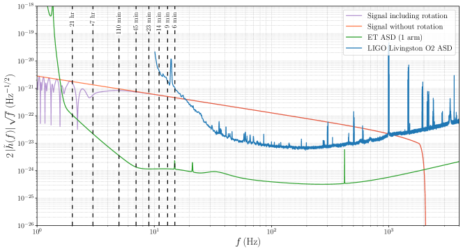
Figure 2: Comparison between the amplitude of a BNS signal analogous to GW170817, as seen by a single instrument of the ET triangular detector (whose sensitivity curve is shown in green) accounting for the effect of Earth’s rotation (violet curve) and without accounting for it (orange curve). The dashed vertical lines indicate the amount of time left before coalescence and the amplitude is computed using the waveform model IMRPhenomD_NRTidalv2. For comparison, we also report in blue a representative LIGO Livingston sensitivity curve during the second observing run, available at https://dcc.ligo.org/LIGO-G1801952/public.

The effect of this location phase is of particular relevance in the case of a network of detectors, since the difference in the arrival time of the signal between different detectors gives a fundamental information to localize the source. The Doppler effect due to the rotation of the Earth around the Sun, which is relevant for instance for LISA, is negligible for the signals expected at ground–based detectors.

In summary, the signal in the frequency domain takes the form

$$\begin{split}\tilde{h}(f)=\Big{[}F_{+}\big{(}t^{\ast}(f);{\bf\it\theta},{\bf\it\lambda}\big{)}\,A^{(F)}_{+}(f,{\bf\it\theta})&+F_{\times}\big{(}t^{\ast}(f);{\bf\it\theta},{\bf\it\lambda}\big{)}\,A^{(F)}_{\times}(f,{\bf\it\theta})\Big{]}\times\\ &\exp{i\left[2\pi ft_{c}+\phi_{L}\left(t^{\ast}(f)\right)-\Phi_{c}+\Phi^{(F)}(f;{\bf\it\theta})-\frac{\pi}{4}\right]}\,,\end{split}$$ (22)

where the quantities $A^{(F)}_{+,\times}(f,{\bf\it\theta})$ and $\Phi^{(F)}(f;{\bf\it\theta})$ are the output of the waveform model in frequency domain [which already includes the factor $(2\pi/\ddot{\Phi}(t^{\ast}))^{\nicefrac{{1}}{{2}}}$ in Eq. (18)], and $\Phi_{c}$ the value of the phase at coalescence, which we explicitly separated from $\Phi^{(F)}(f;{\bf\it\theta})$ for clarity.

When including the contribution of higher modes, the signal can be expressed as a superposition of multipoles of spin–weighted spherical harmonics (Goldberg et al., 1967) of weight $-2$, whose Fourier transform can be computed independently. To compute the frequency–domain signal one can thus proceed as before, obtaining

$$\begin{split}\tilde{h}(f,{\bf\it\theta},{\bf\it\lambda})=\Big{[}F_{+}(t^{\ast}(f),{\bf\it\theta},{\bf\it\lambda})\,\tilde{h}_{+}(f,{\bf\it\theta})&+F_{\times}(t^{\ast}(f),{\bf\it\theta},{\bf\it\lambda})\,\tilde{h}_{\times}(f,{\bf\it\theta})\Big{]}\times\\ &\exp{i\left[2\pi ft_{c}+\phi_{L}\left(t^{\ast}(f)\right)-\Phi_{c}-\frac{\pi}{4}\right]}\,,\end{split}$$ (23)

where the quantities $\tilde{h}_{+,\times}$ are now the output of the waveform model, computed in frequency domain [see e.g. García-Quirós et al. (2020)] as

$$\tilde{h}_{+}(f,{\bf\it\theta}) =\sum_{\ell\geq 2}\sum_{m=0}^{\ell}\dfrac{1}{2}\left[{}_{-2}Y_{\ell m}(\iota)+(-1)^{\ell}_{-2}Y_{\ell-m}^{\ast}(\iota)\right]A^{(F)}_{\ell m}(f,{\bf\it\theta})\exp{i\Phi^{(F)}_{\ell m}(f,{\bf\it\theta})},$$ (24)

$$\tilde{h}_{\times}(f,{\bf\it\theta}) =\sum_{\ell\geq 2}\sum_{m=0}^{\ell}\dfrac{i}{2}\left[{}_{-2}Y_{\ell m}(\iota)-(-1)^{\ell}_{-2}Y_{\ell-m}^{\ast}(\iota)\right]A^{(F)}_{\ell m}(f,{\bf\it\theta})\exp{i\Phi^{(F)}_{\ell m}(f,{\bf\it\theta})}\,,$$

with $A^{(F)}_{\ell m}$ and $\Phi^{(F)}_{\ell m}$ being the amplitude and phase of the $(\ell,m)$ mode in frequency domain.

Another noteworthy aspect is that, when using a triangular–shaped detector, like ET (see Sect. 4.2 for a brief description of its design), it is not needed to compute the signal in each interferometer, since the sum of all the signals will vanish by geometrical reasons (Freise et al., 2009). In fact, the difference among the signals observed in each instrument will arise only from the pattern functions, that depend on the orientation of the detector as

$$F_{n}\propto C_{1}\sin\left(2\gamma+n\dfrac{2\pi}{3}\right)+C_{2}\cos\left(2\gamma+n\dfrac{2\pi}{3}\right);\qquad n\in\{1,2,3\},$$ (25)

where $\gamma$ denotes the orientation of the first interferometer (the angle between east and the bisector of the first arm in the expressions we use) and the terms $C_{1}$ and $C_{2}$ collect all the other terms appearing in the pattern functions. We here assumed the three interferometers to be equal and co–located, which is a sensible approximation for ground–based detectors. It can then be trivially shown that $F_{1}+F_{2}+F_{3}=0$, thus the signal in one of the instruments can simply be obtained from the signals in the other two, reducing the amount of needed calculations by one third. This is the basis of the so–called null–stream, that is the data stream obtained by summing the signals in the instruments of a closed–loop detector, and offers outstanding capabilities for analysing data (Gürsel & Tinto, 1989; Wen & Schutz, 2005; Ajith et al., 2006; Chatterji et al., 2006; Rakhmanov, 2006; Harry & Fairhurst, 2011; Regimbau et al., 2012; Schutz & Sathyaprakash, 2020; Wong et al., 2021; Wong & Li, 2022). In particular, as it has recently be shown in Goncharov et al. (2022) , it can be used to eliminate glitches contaminating the detector data stream, and to get unbiased estimates of the power spectral density (PSD). Notice also that the null–stream in ET corresponds to the so–called T channel of the LISA space interferometer (Prince et al., 2002).

3.3 Technical aspects

We here briefly outline some technical choices made to implement the above features in GWFAST, which are described in more detail, and tested, in the companion paper Iacovelli et al. (2022). GWFAST is a pure Python code that fully exploits the vectorization capabilities of this language, and is able to rapidly get signal–to–noise ratios and Fisher matrices for large catalogs of events. In particular, we entirely re–wrote in Python, in fully vectorized form, the waveform models IMRPhenomD, IMRPhenomD_NRTidalv2, IMRPhenomHM and IMRPhenomNSBH, available in C in the LIGO Algorithm Library, LAL (LIGO Scientific Collaboration, 2018). Together with this paper and GWFAST, we also release the open–source library WF4Py containing the Python implementation of the waveforms. The agreement with LAL is excellent, at the level of $\sim 10^{-14}$ in the inspiral part and $\sim 10^{-5}$ in the worst case in the merger–ringdown. The difference in the latter case is entirely due to interpolation routines needed to compute the waveform in the ringdown phase. GWFAST anyway also implements an interface with LAL, which makes possible to easily use all the waveforms available in that library.

When using pure Python waveforms, derivatives in GWFAST are computed using a mixture of analytical differentiation and automatic differentiation. The latter is a technique alternative to finite–difference, that allows us to compute derivatives up to machine precision without issues of convergence due to the step–size choice in finite difference, based on a decomposition of the function in elementary functions, see Margossian (2018) for a review. In particular, GWFAST makes use of the implementation in the JAX package (Bradbury et al., 2018). This further has the advantage of allowing vectorization of the computation of derivatives, thus fully exploiting the capabilities of Python. For this to be efficient, a vectorized implementation of the waveforms is needed, which motivated the development of WF4Py. Finally, differentiation with respect to the parameters $d_{L},\ \theta,\ \phi,\ \iota,\ \psi,\ t_{c}$ and $\Phi_{c}$, which do not depend on the waveform model, is implemented analytically, to further gain in speed and accuracy. As additional checks of reliability, we verified that, for these parameters, the analytical results and the result obtained by JAX agree at machine precision ($10^{-15}$ in our case). We also implemented the FIM formalism in an independent code in Wolfram Mathematica in the case of the TaylorF2_RestrictedPN waveform model, for which the calculation of all derivatives can be more easily performed analytically. The agreement on the diagonal elements is never worse than $10^{-4}$, including differences in the integration routines in the two languages. We refer to Iacovelli et al. (2022) for more details of these tests.

When resorting instead to the LAL waveforms, the computation of the derivatives is performed using finite difference techniques, as implemented in the numdifftools library, with an adaptive step–size, while the differentiation with respect to the parameters $d_{L},\ \theta,\ \phi,\ \iota,\ \psi,\ t_{c}$ and $\Phi_{c}$, is still performed analytically.

Coming to the inversion of the FIM, each row and column is normalized to the square root of the diagonal entries, so that the resulting matrix has ones on the diagonal and the remaining elements in the interval $[-1,\,1]$ (Harms et al., 2022). This transformation is applied again after the inversion of the resulting matrix to obtain the inverse of the original FIM. The inversion itself is done by means of the Cholesky decomposition, which amounts to express a (hermitian, positive–definite) matrix as a product of a lower triangular matrix and its conjugate transpose. The inversion of a triangular matrix is an easier task than that of a full matrix, which improves the inversion. Other methods supported by GWFAST are discussed in Iacovelli et al. (2022). The inversion makes use of the Python library mpmath for precision arithmetic.

4 Applications to current and future ground–based detectors

In this section, we use GWFAST to study the detection and parameter estimation capabilities of current and future observatories for the three kind of GW sources that have been detected so far, namely, BBHs, BNSs, and NSBHs. The goal is to give realistic forecasts based on updated population models. For the short term, we focus on the forthcoming O4 run of the LIGO–Virgo–KAGRA (LVK) collaboration. For the long term, we consider a single Einstein Telescope (ET) observatory, and a network “ET+2CE”, made by ET, located in Europe, and two Cosmic Explorers (CE), located in the US.

4.1 Populations

We here describe our baseline assumptions for the populations of the three kinds of compact binary systems considered in the analysis, (astrophysical) BBHs, BNSs and NSBHs, also summarised in Tab. 1. The functional form and numerical values of the parameters for all distributions are reported in App. A.

BBH

We adopt a source–frame mass and spin distribution calibrated on the latest LVK results (Abbott et al., 2021c), using the Power Law + Peak profile for the former, and the Default model for the latter, and assume that the mass and spin distributions do not evolve with redshift. For the local rate, the value inferred from the GWTC–3 catalog is ${\cal R}_{0,{\rm BBH}}=17^{+10}_{-6.7}\leavevmode\nobreak\ ${\mathrm{Gpc}}^{-3}\text{\,}{\mathrm{yr}}^{-1}$$. We will then adopt ${\cal R}_{0,{\rm BBH}}=$17\text{\,}{\mathrm{Gpc}}^{-3}\text{\,}{\mathrm{yr}}^{-1}$$ as our reference value. Given the still limited redshift range of the detected events, the rate distribution in redshift has large uncertainties, and only its power-law behavior at low redshift has been constrained. Since 3G detectors will cover a much broader redshift range, for which a power–law behavior is not realistic, we choose to adopt a Madau–Dickinson profile (Madau & Dickinson, 2014) in which the low–end slope is fixed to the LVK value and the other parameters assume typical values used in the literature (Madau & Fragos, 2017), see App. A for details. With these choices, we find that the number of BBHs coalescing in one year, out to $z=20$, is $N_{\rm BBH}\simeq$7.5\text{\times}{10}^{4}$$.

Several caveats are here in order. Beside the uncertainty in the local rate (see Mandel & Broekgaarden (2022) for a comprehensive review of the uncertainties from both observation and theory), there is an uncertainty on the BBH mass function, for which the LVK data already provide some information, but which can still vary significantly; even more important are the uncertainties on the redshift evolution of the merger rate (Dominik et al., 2013; Santoliquido et al., 2021a; Rozner & Perets, 2022; Chruślińska, 2022) and of the mass and spin distributions. For the redshifts of interest at 3G detectors, these distributions cannot be significantly constrained by current data, while theoretical modelizations still have large uncertainties. Our choice of neglecting any redshift dependence in the mass and spin distributions is the simplest one, and is consistent with Abbott et al. (2021c), that find no evidence for redshift dependence in the range of redshifts currently explored by 2G detectors. For the broader range of redshifts that will be accessible to 3G detectors, this is not expected to continue to hold, see e.g. Fishbach et al. (2021); van Son et al. (2022); Belczynski et al. (2022) for the redshift dependence of the mass distribution, and Qin et al. (2018); Biscoveanu et al. (2022); Bavera et al. (2022) for the redshift dependence of the spin distribution. Our choice of redshift–independent mass and spin distributions should therefore be considered only as dictated by simplicity, and will likely have to be modified as the observational and theoretical understanding improve. It should also be stressed that, already for BBHs of astrophysical origin, different formation channels have merger rates with different redshift dependence; in particular, BBHs whose progenitors were population III stars have a redshift dependence of the merger rate which is sensibly different from the one that we have assumed, and can extend to redshift $z\sim 20$ and beyond, see Kinugawa et al. (2014); Ng et al. (2021a) and references therein. Furthermore, BBHs with a primordial origin would have a completely different merger rate, that increases monotonically with redshift as $R_{\rm PBH}\propto[t(z)]^{-\nicefrac{{34}}{{37}}}$ up to $z=\order{${10}^{3}$}$ (Raidal et al., 2019; De Luca et al., 2020, 2021a), see also Franciolini (2021) for recent review.

BNS

The knowledge of the population of merging BNS binaries is still limited compared to BBH systems, given the very small number of GW detections of this class of sources. Following Abbott et al. (2021f, c), we assume that the (source–frame) masses of neutron stars in merging binaries have a flat distribution in the interval $[1,2.5]\,$\mathrm{M_{\odot}}$$. The other distribution commonly used in the literature is a Gaussian for each of the two NSs, such as $\mathcal{N}(\mu=1.33,\sigma=0.09)$ (with masses in units of $\mathrm{M_{\odot}}$), which comes from galactic electromagnetic (EM) observations (Farrow et al., 2019). The local rate for BNS mergers inferred from GW observations is quite sensitive to the assumptions made for the mass function distribution, and it is therefore important to choose a rate consistent with the assumed mass distribution. The value inferred from the GWTC–3 catalog, assuming a flat mass distribution, is ${\cal R}_{0,\rm BNS}=105.5^{+190.2}_{-83.0}\leavevmode\nobreak\ ${\mathrm{Gpc}}^{-3}\text{\,}{\mathrm{yr}}^{-1}$$ (Abbott et al., 2021c). In the following, we will then use as reference value ${\cal R}_{0,\rm BNS}=$105.5\text{\,}{\mathrm{Gpc}}^{-3}\text{\,}{\mathrm{yr}}^{-1}$$. However, the uncertainty on this number is still quite large and, depending on the astrophysical modelization used, values of ${\cal R}_{0,\rm BNS}$ in the range $(10-1700)\leavevmode\nobreak\ ${\mathrm{Gpc}}^{-3}\text{\,}{\mathrm{yr}}^{-1}$$ are consistent with current observations (Abbott et al., 2021c). We will emphasize this uncertainty whenever we quote numbers that depend on the local BNS rate. With our choices, the number of BNSs coalescing in one year, out to $z=20$, is $N_{\rm BNS}\simeq$1\text{\times}{10}^{5}$$.

Given the expected small values for the spins of these objects, we sample their components aligned with the orbital angular momentum independently and uniformly in the range $[-0.05,\,0.05]$. Another parameter characterising NSs is the adimensional tidal deformability, $\Lambda$, which strongly depends on the equation of state (EoS) of dense matter above the nuclear density, and is still largely unknown (Hinderer et al., 2010). We thus make the agnostic choice of sampling $\Lambda$ for each component uniformly in the range $[0,\,2000]$, which is compatible with current observations (Abbott et al., 2019a, 2020a). In App. D we compare with the results obtained by using some specific NS equations of state. For the redshift distribution of these systems we assume a Madau–Dickinson profile convolved with a time delay distribution $P(t_{d})\propto 1/t_{d}$ with a minimum time delay of $20\text{\,}\mathrm{Myr}$, which is again a standard choice in the literature [see e.g. Regimbau et al. (2012); Belgacem et al. (2019a)] and, again, no redshift evolution for the mass distribution.

NSBH

The population of this class of sources is the most uncertain, with only two GW observations by the time of writing (Abbott et al., 2021g), and no electromagnetic observation. For the NS we adopt a Gaussian distribution for the masses, $\mathcal{N}(1.33,0.09)$ (with masses in units of $\mathrm{M_{\odot}}$), which seems a good approximation to realistic astrophysical scenarios [see e.g. Fig. 14 of (Broekgaarden et al., 2021)], an aligned spin uniformly distributed in the interval $[-0.05,\,0.05]$, and an adimesional tidal deformability parameter uniformly sampled in $[0,\,2000]$. Both from observations and astrophysical simulations, there seems to be a preference for low–mass BHs appearing in this systems, also with small spins. We thus adopt for the BH mass distribution the fitting function provided in Eq. (6) of Jin-Ping et al. (2021), which is tuned on the astrophysical simulations of Giacobbo & Mapelli (2018), and shows a peak around $m_{\rm BH}\sim$8\text{\,}$Msun{\mathrm{M_{\odot}}}$$$, while for the BH aligned spin component we assume a Gaussian distribution $\mathcal{N}(0,0.15)$ as suggested in Jin-Ping et al. (2021), which is consistent with the values found in the analysis of GW200105 and GW200115. The rate distribution is the most uncertain, as can be seen for example from the various plots and discussion in Santoliquido et al. (2021b); Broekgaarden et al. (2021). We thus adopt the same distribution used in the BNS case, i.e. a Madau–Dickinson profile convolved with a time delay distribution $P(t_{d})\propto 1/t_{d}$ with a minimum time delay of $20\text{\,}\mathrm{Myr}$. With these choices, the number of merger per year out to $z=20$ is $N_{\rm NSBH}\simeq$4.5\text{\times}{10}^{4}$$. We will then study the dependence of our results on these choices for the BH mass distribution and the event rate, comparing with some of the models presented in Broekgaarden et al. (2021).

The assumptions for the remaining parameters are common to all the three kinds of sources: the non–aligned spin components are set to 0, the sky position parameters $\theta$ and $\phi$ are sampled uniformly over the whole sphere, the cosine of the inclination angle is sampled uniformly in the interval $[-1,\,1]$, while the polarisation angle in the interval $[0,\,\pi]$, and coalescence phase in $[0,\,2\pi]$, and the time of coalescence is sampled uniformly in time over a 10 year period. The luminosity distances are computed from the redshifts assuming a flat $\Lambda$CDM cosmology with Planck18 parameters (Planck Collaboration et al., 2020), using the astropy.cosmology package (Price-Whelan et al., 2018).

Parameter	BBH	BNS	NSBH
$m_{1}$	Power Law + Peak (Abbott et al., 2021c)	uniform in $[1,\,2.5]$ $\mathrm{M_{\odot}}$	(Jin-Ping et al., 2021) Eq. (6)
$m_{2}$			$\mathcal{N}(1.33,0.09)$ in $\mathrm{M_{\odot}}$
$z$	Madau–Dickinson (Madau & Dickinson, 2014)	Madau–Dickinson + $P(t_{d})\propto 1/t_{d}$, $t_{d,{\rm min}}=$20\text{\,}\mathrm{Myr}$$
$d_{L}$	computed from $z$ assuming Planck18 flat $\Lambda$CDM (Planck Collaboration et al., 2020)
$\chi_{1,z}$	Default (Abbott et al., 2021c)	uniform in $[-0.05,\,0.05]$	$\mathcal{N}(0,0.15)$
$\chi_{2,z}$			uniform in $[-0.05,\,0.05]$
$\chi_{x},\chi_{y}$	0
$\Lambda_{1}$	0	uniform in $[0,\,2000]$	0
$\Lambda_{2}$			uniform in $[0,\,2000]$
$\theta$	$\cos(\theta)$ uniform in $[-1,\,1]$
$\phi$	uniform in $[0,\,2\pi]$
$\iota$	$\cos(\iota)$ uniform in $[-1,\,1]$
$\psi$	uniform in $[0,\,\pi]$
$t_{c}$	uniform in 10 yr
$\Phi_{c}$	uniform in $[0,\,2\pi]$

Table 1: Summary of the distributions assumed for all the parameters of the three classes of compact binary systems considered, refer to the the text for more details. For BBHs and BNSs the index 1 refer to the heaviest component and the index 2 to the lightest. For NSBH systems the index 1 refers to the BH and the index 2 to the NS.

4.2 Detector networks

Detector	arms length	latitude $\lambda$	longitude $\varphi$	orientation $\gamma$	arms aperture $\zeta$	shape	duty cycle
CE 1	$40\text{\,}\mathrm{km}$	$46.5\text{\,}\mathrm{\SIUnitSymbolDegree}$	$-119.4\text{\,}\mathrm{\SIUnitSymbolDegree}$	$171\text{\,}\mathrm{\SIUnitSymbolDegree}$	$90\text{\,}\mathrm{\SIUnitSymbolDegree}$	L	85%
CE 2	$20\text{\,}\mathrm{km}$	$30.6\text{\,}\mathrm{\SIUnitSymbolDegree}$	$-90.8\text{\,}\mathrm{\SIUnitSymbolDegree}$	$242.7\text{\,}\mathrm{\SIUnitSymbolDegree}$	$90\text{\,}\mathrm{\SIUnitSymbolDegree}$	L	85%
ET	$10\text{\,}\mathrm{km}$	$40.5\text{\,}\mathrm{\SIUnitSymbolDegree}$	$9.4\text{\,}\mathrm{\SIUnitSymbolDegree}$	$0\text{\,}\mathrm{\SIUnitSymbolDegree}$	$60\text{\,}\mathrm{\SIUnitSymbolDegree}$	Triangle	85%
LIGO H1	$4\text{\,}\mathrm{km}$	$46.5\text{\,}\mathrm{\SIUnitSymbolDegree}$	$-119.4\text{\,}\mathrm{\SIUnitSymbolDegree}$	$171\text{\,}\mathrm{\SIUnitSymbolDegree}$	$90\text{\,}\mathrm{\SIUnitSymbolDegree}$	L	70%
LIGO L1	$4\text{\,}\mathrm{km}$	$30.6\text{\,}\mathrm{\SIUnitSymbolDegree}$	$-90.8\text{\,}\mathrm{\SIUnitSymbolDegree}$	$242.7\text{\,}\mathrm{\SIUnitSymbolDegree}$	$90\text{\,}\mathrm{\SIUnitSymbolDegree}$	L	70%
Virgo	$3\text{\,}\mathrm{km}$	$43.6\text{\,}\mathrm{\SIUnitSymbolDegree}$	$10.5\text{\,}\mathrm{\SIUnitSymbolDegree}$	$115.6\text{\,}\mathrm{\SIUnitSymbolDegree}$	$90\text{\,}\mathrm{\SIUnitSymbolDegree}$	L	70%
KAGRA	$3\text{\,}\mathrm{km}$	$36.4\text{\,}\mathrm{\SIUnitSymbolDegree}$	$137.3\text{\,}\mathrm{\SIUnitSymbolDegree}$	$15.4\text{\,}\mathrm{\SIUnitSymbolDegree}$	$90\text{\,}\mathrm{\SIUnitSymbolDegree}$	L	70%

Table 2: Summary of the positions, orientations, angle between arms, shapes and duty cycles of the detectors used in our analysis. The orientation denotes the angle between the bisector of the arms (the first arm in the case of a triangle) and East.

Our analysis is carried out for three different networks of detectors, which are also summarised in Tab. 2:

LVK O4

This network consists of the four L–shaped ground–based GW detectors which are operative at the time of writing, namely the two LIGO detectors, in the U.S., in the sites of Hanford and Livingston, Virgo, in Italy, near Cascina, and KAGRA, in Japan, near Hida. The expected PSDs for all the detectors can be downloaded from https://dcc.ligo.org/LIGO-T2000012/public. To forecast the capabilities of the O4 observational run we use the Advanced LIGO sensitivity with a BNS range of $190\text{\,}\mathrm{Mpc}$, the Advanced Virgo sensitivity with a BNS range of $120\text{\,}\mathrm{Mpc}$, and the KAGRA sensitivity with a BNS range of $10\text{\,}\mathrm{Mpc}$, which corresponds to current expectations for the best sensitivities that could be reached during O4. To be more realistic, we produce our results assuming an uncorrelated 70% duty cycle for each detector, as suggested in Abbott et al. (2020b).

ET

Einstein Telescope (ET) is a proposed third generation GW detector, to be built in Europe. A candidate site is in the municipality of Lula, in Sardinia, Italy, and we use this location for definiteness. Very similar results would be obtained choosing the candidate site in the Meuse–Rhine Euroregion, across the borders of the Netherlands, Belgium and Germany (basically, the only difference is in the effect of the Earth’s rotation on the localization capability of BNSs, that slightly improves increasing the latitude). Differently from current detectors, ET will be an underground detector and has a triangular design, consisting of three nested interferometer with $10\text{\,}\mathrm{km}$ long arms forming angles of $60\text{\,}\mathrm{\SIUnitSymbolDegree}$. Each interferometer actually has a xylophone design, meaning that each arm will consist of two separate instruments, one optimised for high frequencies and one for low frequencies. For our purposes they can be treated effectively as three equal co–located detectors rotated by $120\text{\,}\mathrm{\SIUnitSymbolDegree}$ with respect to each other, neglecting the distance between each arm. The official ET PSD (corresponding to what was formerly called the ET–D design) can be downloaded at https://apps.et-gw.eu/tds/?content=3&r=14065. We also assume an uncorrelated duty cycle of 85% for each arm of the detector, as in Ronchini et al. (2022).

ET + 2CE

Beside ET alone, we will study a network of three 3G ground–based detectors, made by ET in Europe, and by two Cosmic Explorer detectors in the U.S. The CE detectors are planned to be L–shaped interferometers, on the surface (rather than underground, as ET). Two main configurations are being investigated, one in which both detectors have $40\text{\,}\mathrm{km}$ arms, and one that consists of a detector with $40\text{\,}\mathrm{km}$ arms and another with $20\text{\,}\mathrm{km}$ arms (Evans et al., 2021). The latter, beside its baseline design (that, for the given length, maximizes the range to compact binaries), can also be occasionally tuned to have a better sensitivity to the post–merger phase of BNSs. The network with a $40\text{\,}\mathrm{km}$ detector and a tunable $20\text{\,}\mathrm{km}$ detector appears to maximize the science output and is currently the reference CE configuration (Evans et al., 2021). We will then study the case in which one CE detector has $40\text{\,}\mathrm{km}$ arms and the other has $20\text{\,}\mathrm{km}$ arms (which we will set in its baseline configuration, that maximizes the range to compact binaries), and we will refer to the network made by ET and these two CE detectors as “ET+2CE”. Given the current uncertainty about their construction sites, for definiteness we assume the $40\text{\,}\mathrm{km}$ interferometer to be located and oriented as the LIGO Hanford detector while the $20\text{\,}\mathrm{km}$ instrument as LIGO Livingston; these are not expected to be the actual locations but, at the level of the present analysis, this will not be very important, as long as their relative distance is comparable to the one assumed here. Another option under consideration, in which one of the two CE detectors could rather be placed in Australia, would of course lead to better angular localization. In our analysis we will not consider the two CE detectors alone (except in the plots showing the range, in Fig. 4 and 5 below), but always a network consisting of them and ET. Again, we assume an uncorrelated 85% duty cycle for the two CE detectors and each arm of ET.

The noise spectral densities of the various detectors considered are shown in Fig. 3. We take into account that ET is made of three nested interferometers, with an opening angle of $60\text{\,}\mathrm{\SIUnitSymbolDegree}$. In the ${\rm SNR}^{2}$, this gives a factor $3\times(\sqrt{3}/2)^{2}=9/4$, i.e. a factor $3/2$ in the SNR. Therefore, to compare with the sensitivity of a single L–shaped interferometer, we multiply the ET sensitivity by a factor $2/3$. In Fig. 4 we show, for LVK during the O4 run, for ET, and for a network of two CE (without ET), the corresponding horizon distance to BBHs (i.e., the maximum distance to which a BBH optimally oriented and with optimal sky location can be detected), requiring ${\rm SNR}\geq 8$ for detection, where SNR is the signal–to–noise ratio of the detector network. The lower edge of the shaded bands gives the distance to which about $50\%$ of the BBHs can be detected. This has been obtained requiring that the SNR, averaged over sky position and inclination, is above our threshold value, which is a proxy for a more accurate computation obtained performing a sampling of a population of events for each mass bin. The left panel shows the case of equal mass and non–spinning binaries, and is analogous to a well–known plot presented in Hall & Evans (2019). In the central panel we show the result for non–spinning binaries with a mass ratio $q=m_{1}/m_{2}=5$, so in this case the fact that we include higher modes matters for the $50\%$ detection range (but not for the horizon, which is obtained for $\iota=0$, in which case the higher modes vanish). Note that, for a given total mass, the horizon decreases by increasing the mass ratio, simply because, for fixed total mass, the chirp mass ${\cal M}_{c}$ decreases as the mass ratio moves away from $q=1$, and the amplitude in the inspiral phase is proportional to ${\cal M}_{c}^{\nicefrac{{5}}{{3}}}$. In the right panel we also turn on the spins, taking aligned spins for the two BHs, choosing for definiteness $\chi_{1,z}=\chi_{2,z}=0.8$, while still keeping $q=5$. We see that the parallel spins have the effect of raising the horizon distance again, because of their repulsive effect in the inspiral phase, which delays the merger (conversely, anti-parallel spins accelerate the merger and lower the horizon distance).

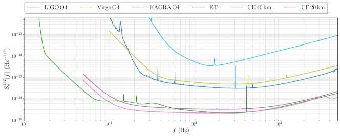
Figure 3: Noise Amplitude Spectral Densities, ASDs, of the various detectors considered. To have a uniform comparison between different geometries, the single–detector ET sensitivity curve has been rescaled by a factor 2/3 to take into account that, having a triangular design, ET actually consists of 3 nested instruments with an opening angle of $60\text{\,}\mathrm{\SIUnitSymbolDegree}$.

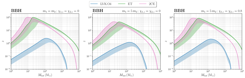
Figure 4: Detection horizons for different monochromatic populations of BBH sources for the LVK detector network during O4, for ET alone, and for a network of two CE detectors (without ET), taken one with 40 km arms and one with 20 km arms. The solid lines show the maximum redshift out to which a binary with optimal sky location and inclination can be detected, while the shaded bands represent the maximum $z$ out to which a binary could be observed after averaging the SNR over the sky, which is a proxy for the redshift out to which $50\%$ of the population with given masses and spins could be detected. We set a detection threshold ${\rm SNR}=8$. In the left panel we show the result for equal mass non–spinning binaries, in the central panel for non–spinning binaries with a mass ratio $q=5$, and in the right panel for binaries with a mass ratio $q=5$ and aligned spin components $\chi_{1,z}=\chi_{2,z}=0.8$. We use the IMRPhenomHM waveform.

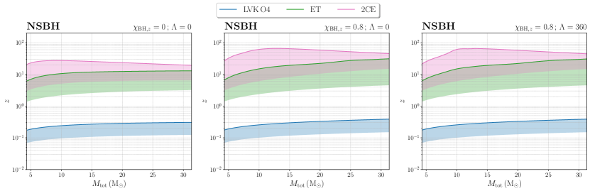
Figure 5: As in Fig. 4 for NSBH sources. The NS mass is fixed to $m_{\rm NS}=$1.33\text{\,}\mathrm{M_{\odot}}$$ while we vary the BH mass in the astrophysically motivated range $[3,\,30]\,$\mathrm{M_{\odot}}$$ (Broekgaarden et al., 2021). In the left panel we show the results for non–spinning binaries neglecting tidal effects; in the central panel for binaries having a BH with aligned spin component $\chi_{{\rm BH},z}=0.8$, and in the right panel we consider both the effect of a spinning BH with $\chi_{{\rm BH},z}=0.8$ and a tidal deformability parameter for the NS $\Lambda=360$, which is consistent with the APR4 (Akmal et al., 1998) soft equation of state. We use the waveform model IMRPhenomNSBH.

For BNS, taking them of equal mass and spinless, which is a very good approximation for actual systems, and neglecting the small effect of tidal deformability, the horizon and $50\%$ detection range can also be read from the left panel of Fig. 4, using a value of $M_{\rm tot}$, such as $M_{\rm tot}\simeq 2.7$, appropriate to typical BNSs.

For NSBHs, instead, the mass ratio is very different from one, and the BH spin is not necessarily small. In Fig. 5 we show the results for NSBH using a horizontal scale for the total mass appropriate to current expectations for these systems, obtained fixing the NS mass to $m_{\rm NS}=$1.33\text{\,}\mathrm{M_{\odot}}$$ and varying the BH mass in the astrophysically motivated range $[3,\,30]\,$\mathrm{M_{\odot}}$$ (Broekgaarden et al., 2021), and using the IMRPhenomNSBH waveform. In the left panel we show the case of a spinless BH, and we set to zero the parameter $\Lambda$ that describes the tidal deformability of the NS. In the central panel we turn on the BH spin (setting, for definiteness, $\chi_{{\rm BH},z}=0.8$) and, in the right panel, we also turn on the NS tidal deformability. We see that, for NSBHs, over the relevant range of masses, the horizon curves are much more flat than for BBHs. This, first of all, is simply due to the much smaller range that we have taken for $M_{\rm tot}$, based on current expectations for NSBH systems. Furthermore, the chirp mass is related to the total mass $M_{\rm tot}$ and to the mass ratio $q=m_{1}/m_{2}$ by ${\cal M}_{c}=[q/(1+q)^{2}]^{\nicefrac{{3}}{{5}}}M_{\rm tot}$. Therefore, for $q\gg 1$, as is the case for NSBHs (recall that, with our conventions, $m_{1}\geq m_{2}$, so $q\geq 1$), we have ${\cal M}_{c}\simeq q^{-\nicefrac{{3}}{{5}}}M_{\rm tot}$ and a given change in $M_{\rm tot}$ results in a smaller change in ${\cal M}_{c}$, which is the mass scale that characterizes the amplitude. We also see that, for CE, increasing $M_{\rm tot}$, beyond some value in the considered range the horizon starts to decrease; this is due to the fact that, increasing $M_{\rm tot}$, the merger takes place at lower frequencies, so the signal is moved toward the region where the sensitivity of CE degrades faster, compared to ET.

5 Results

We now show the results of our analysis for the three populations of sources, as seen by the different detector networks and with the assumptions discussed above. We first compute, for each event, the network SNR, defined by

$${\rm SNR}^{2}=\sum\nolimits_{i}{\rm SNR}^{2}_{i}\,,$$ (26)

where the sum runs over the detectors, and the matched filter signal–to–noise ratios ${\rm SNR}_{i}$ of the individual detectors are given in Eq. (5) or, more explicitly,

$${\rm SNR}^{2}_{i}=4\int_{f_{\rm min}}^{f_{\rm cut}}\dfrac{|\tilde{h}_{(i)}(f)|^{2}}{S_{n,i}(f)}\differential{f}\,.$$ (27)

Here $\tilde{h}_{(i)}(f)$ denotes the GW signal as detected by the $i^{\rm th}$ detector in the network (thus including the contribution of the pattern function of the detector and the location phase factor), $S_{n,i}(f)$ is the one–sided noise PSD of the $i^{\rm th}$ detector, $f_{\rm min}$ denotes the minimum frequency of the adopted frequency grid, which we set at $2\text{\,}\mathrm{Hz}$ for ET, $5\text{\,}\mathrm{Hz}$ for CE and $10\text{\,}\mathrm{Hz}$ for 2G detectors, and $f_{\rm cut}$ is the maximum frequency of the grid, which depends on the source characteristics and the adopted waveform model. After the SNRs have been determined, we perform a Fisher analysis restricting to the events having a network ${\rm SNR}\geq 12$ (in the case of ET, the network SNR is obtained combining the contributions of the three arms). We will also compare the results for the number of detections and horizon distances with the results obtained with a network ${\rm SNR}\geq 8$, while not performing a Fisher matrix analysis in this case, since it becomes less reliable for such low values of the SNR.

We further discard the signals with an inversion error of the Fisher matrix bigger than $5\times 10^{-2}$ (see Sect. 2.2). The Fisher matrices are computed according to Eq. (6). For a network of detectors, the total Fisher matrix is just the sum of the Fisher matrices computed for each detector. For BBHs the set of parameters is ${\bf\it\theta}=\{{\cal M}_{c},\ \eta,\ d_{L},\ \theta,\ \phi,\ \iota,\ \psi,\ t_{c},\ \Phi_{c},\ \chi_{1},\ \chi_{2}\}$, where we denoted the aligned spin components, $\chi_{1,z}$ and $\chi_{2,z}$, simply as $\chi_{1}$ and $\chi_{2}$, to simplify the notation. For BNS and NSBH systems, ${\bf\it\theta}$ also includes the tidal deformability parameters $\tilde{\Lambda}$ and $\delta\tilde{\Lambda}$, defined in Eq. (14), where, in the case of NSBH, the parameter $\Lambda_{1}$ corresponding to the BH must be set to zero (recall, from Tab. 1, that for NSBH we use the convention that the index $i=1$ always refers to the BH). After the inversion of the Fisher matrix, we compute the sky localization area for the events according to the definition (Barack & Cutler, 2004; Wen & Chen, 2010)

$$\Delta\Omega_{{\rm X}\%}=-2\pi|\sin\theta|\mathchoice{{\hbox{$\displaystyle\sqrt{\left(\Gamma^{-1}\right)_{\theta\theta}\,\left(\Gamma^{-1}\right)_{\phi\phi}-\left(\Gamma^{-1}\right)_{\theta\phi}^{2}\,}$}\lower 0.4pt\hbox{\vrule height=9.30444pt,depth=-7.44359pt}}}{{\hbox{$\textstyle\sqrt{\left(\Gamma^{-1}\right)_{\theta\theta}\,\left(\Gamma^{-1}\right)_{\phi\phi}-\left(\Gamma^{-1}\right)_{\theta\phi}^{2}\,}$}\lower 0.4pt\hbox{\vrule height=9.30444pt,depth=-7.44359pt}}}{{\hbox{$\scriptstyle\sqrt{\left(\Gamma^{-1}\right)_{\theta\theta}\,\left(\Gamma^{-1}\right)_{\phi\phi}-\left(\Gamma^{-1}\right)_{\theta\phi}^{2}\,}$}\lower 0.4pt\hbox{\vrule height=6.53888pt,depth=-5.23112pt}}}{{\hbox{$\scriptscriptstyle\sqrt{\left(\Gamma^{-1}\right)_{\theta\theta}\,\left(\Gamma^{-1}\right)_{\phi\phi}-\left(\Gamma^{-1}\right)_{\theta\phi}^{2}\,}$}\lower 0.4pt\hbox{\vrule height=5.03888pt,depth=-4.03113pt}}}\ \ln{\left(1-\dfrac{{\rm X}}{100}\right)}\,,$$ (28)

where X denotes the confidence level. The result of this expression is in units of steradian, so a further multiplication by $($180\text{\,}\mathrm{\SIUnitSymbolDegree}$/\pi)^{2}$ is needed to get the estimation in the usual ${\mathrm{deg}}^{2}$ units. We will give our results in terms of $\Delta\Omega_{90\%}$.

5.1 Binary black holes

We first focus on BBH systems, which are on average the loudest signals that can be observed in the frequency band of current and future ground–based detectors. As recalled in Sect. 4.1, the most recent estimate for the local rate from the GWTC–3 catalog is ${\cal R}_{0,{\rm BBH}}=17^{+10}_{-6.7}\leavevmode\nobreak\ ${\mathrm{Gpc}}^{-3}\text{\,}{\mathrm{yr}}^{-1}$$ (Abbott et al., 2021c), so we use the value ${\cal R}_{0,{\rm BBH}}=17\leavevmode\nobreak\ ${\mathrm{Gpc}}^{-3}\text{\,}{\mathrm{yr}}^{-1}$$ as our reference value for normalizing the redshift distribution of the merger rate discussed in App. A. In particular, this means that our merger rate as a function of redshift, ${\cal R}_{{\rm BBH}}(z)$, will be consistent with that shown in Fig. 13 of Abbott et al. (2021c). For these systems we simulate a population of $N_{\rm BBH}=$7.5\text{\times}{10}^{4}$$ sources out to $z=20$ that, as mentioned in Sect. 4.1, using this value for ${\cal R}_{0,{\rm BBH}}$ and our choice for the redshift distribution of the merger rate, corresponds to the number of systems coalescing in one year.

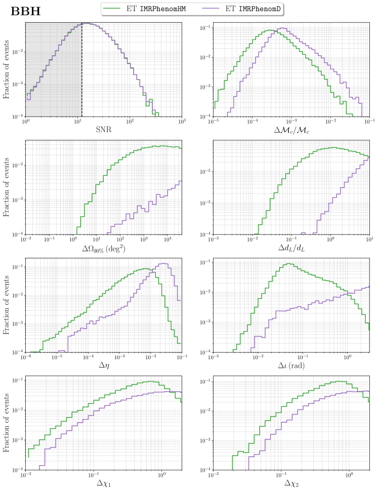
Figure 6: Histograms of the SNR and parameter errors for BBHs for ET alone, using the waveform model IMRPhenomHM, which includes sub–dominant modes of the signal, and IMRPhenomD, which only contains the quadrupole. For the SNR, in each bin we show the fraction of events, normalized to the total number of sources in our sample. For the parameters of the waveform, we limit to the $\tilde{N}_{\rm det}$ events that pass the cut ${\rm SNR}\geq 12$, and that furthermore admit a reliable inversion of the Fisher matrix, and we show the fraction of events, normalized to $\tilde{N}_{\rm det}$.

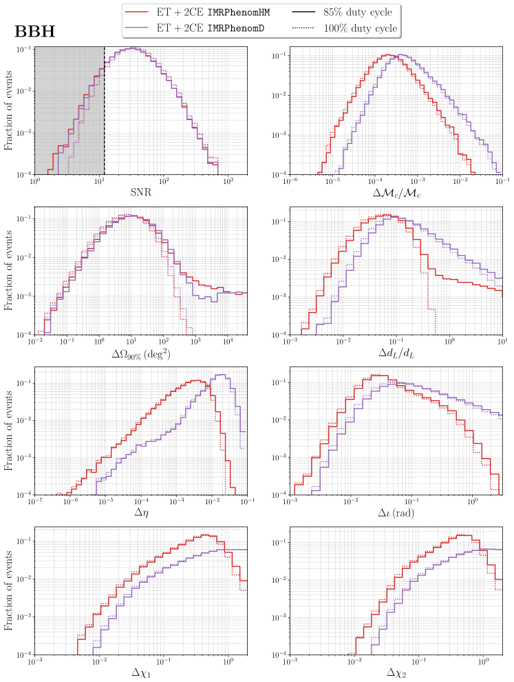
Figure 7: As in Fig. 6, for the ET+2CE network. We here further show the results obtained without imposing the 85% uncorrelated duty cycle for the detectors.

At the methodological level, it is important first of all to understand the effect of the waveform model used and, in particular, for heavy systems such as BBHs, the role of higher modes. We then begin by comparing the results obtained using IMRPhenomHM, which is our baseline waveform for BBHs and, as discussed in Sect. 3.1, includes several higher modes, with the results that we get analysing the same catalog of sources with the waveform model IMRPhenomD (Husa et al., 2016; Khan et al., 2016a). This is a full inspiral–merger–ringdown model, tuned to binaries with non–precessing spins but, differently from IMRPhenomHM, it only contains the dominant quadrupole mode of the signal. The results are shown in Fig. 6 for ET alone and in Fig. 7 for ET+2CE. In the upper left panels of these figures we show, for the two waveforms, the distribution in SNR of the whole sample of events, displayed as a fraction of events with respect to the total number of events in the sample, i.e. the $7.5\text{\times}{10}^{4}$ sources that we have simulated. We then restrict parameter estimation to the events that pass the cut ${\rm SNR}\geq 12$, which is our criterion for detection and, for these, we perform the Fisher matrix analysis. As discussed in Sect. 2.2, for some of these events the Fisher matrix is ill–conditioned and its inversion can lead to large amplification of numerical errors, resulting in a covariance matrix that can be inaccurate even at the $100\%$ level, and our strategy is to simply discard these events, accepting this as a limitation of the Fisher matrix formalism. We denote by $N_{\rm det}$ the number of events detected in our sample, i.e. those that pass the cut ${\rm SNR}\geq 12$, and by $\tilde{N}_{\rm det}$ the number of detected event that, furthermore, have a Fisher matrix that can be inverted reliably, according to our criterion discussed in Sect. 2.2. In the plots showing the distribution of the errors on the parameters we only include these $\tilde{N}_{\rm det}$ events. The corresponding panels in Fig. 6 and 7, as well as all similar plots in the following, show the distribution of these events, as a fraction normalized to $\tilde{N}_{\rm det}$.

From Fig. 6 we see that, for ET alone, while the distribution of SNR is unaffected by the inclusion of higher modes, parameter estimation is significantly improved. This is especially remarkable for the angular resolution and for the error on the luminosity distance, where the inclusion of higher–order modes allows us to break the distance–inclination degeneracy, but the estimation of all parameters is significantly improved, thanks to the better description offered by the waveform model. For all parameters shown, the inclusion of higher modes has the effect of increasing the fraction of events for which accurate parameter reconstruction is possible, and also of cutting the long tails corresponding to events with large errors, as especially evident in $\Delta\iota$ and $\Delta\eta$. For ET+2CE we see from Fig. 7 that a rather similar pattern emerges, except for the angular localization which, in this case, is completely dominated by the triangulation, rather than by the accuracy of the waveform. Another interesting information that emerges from Fig. 7 is the role of the duty cycle. The dashed lines show the results obtained assuming a $100\%$ duty cycle, while the solid line use a more realistic independent duty cycle of $85\%$ for each detector. We see that the duty cycle has a large effect on the tails of the distribution of $\Delta d_{L}/d_{L}$, and of $\Delta\Omega_{90\%}$. This is natural, since these are the quantities that are more directly sensitive to the network SNR, which decrease when one or more detectors in the network is down. This highlights the importance of having detectors with a high duty cycle, or of having a network of more detectors.

In the following, we therefore focus only on the results obtained using IMRPhenomHM. While a histogram of detection fractions contains the information in its most raw form, the corresponding cumulative distributions give information that is more condensed and often easier to interpret (and less sensitive to the specific random realization used, when small numbers are involved). In Fig. 8 we then show, for LVK–O4, ET alone, and ET+2CE, the corresponding cumulative distributions function (CDF). For the SNR, we show the cumulative distribution of the fraction of events, where the fraction is obtained normalizing the events in a given bin to the total number of events that we have generated; for the other panels, involving parameter estimation, we show the cumulative distribution of the fraction of events obtained normalizing the events in a given bin to $\tilde{N}_{\rm det}$, i.e. to the total number of detected events which, furthermore, admit a reliable inversion of the Fisher matrix. For the SNR we actually plot $1-{\rm CDF}$, so the vertical axis gives the fraction of events with signal–to–noise ratio larger than a given value, while for the parameters we show the CDF, so the fraction of events with error smaller than a given value.

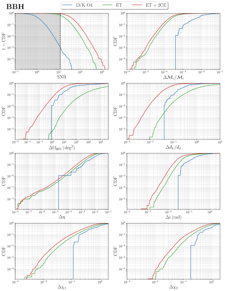
Figure 8: Cumulative distributions of the detection efficiency, for the SNRs and for the error on the parameters, for BBH signals with the three considered network configuration, using the waveform model IMRPhenomHM.

We find that ET alone can detect $67\%$ of the BBH population, while a network of ET and 2CE could detect $93\%$ of the full population of sources. With our reference value for the local rate, ${\cal R}_{0,{\rm BBH}}=$17\text{\,}{\mathrm{Gpc}}^{-3}\text{\,}{\mathrm{yr}}^{-1}$$, a threshold in signal–to–noise ratio ${\rm SNR}\geq 12$, and our choices for the BBH mass function and merger rate distribution in redshift, discussed in Sect. 4.1, this means, for ET alone, that the number of events detected in one year is $N_{\rm det}\simeq$5.1\text{\times}{10}^{4}$$ while, for ET+2CE, the number of BBH events detected per year is $N_{\rm det}\simeq$7.0\text{\times}{10}^{4}$$. Using, more generally, the currently $90\%$ c.l. allowed range ${\cal R}_{0,{\rm BBH}}=[10.3,27]\leavevmode\nobreak\ ${\mathrm{Gpc}}^{-3}\text{\,}{\mathrm{yr}}^{-1}$$ for the local rate, the number of detections per year for ET is in the range $[$3.1\text{\times}{10}^{4}$,$8.0\text{\times}{10}^{4}$]$ and, for ET+2CE, is in the range $[$4.2\text{\times}{10}^{4}$,$1.1\text{\times}{10}^{5}$]$. For LVK in the O4 observational run, we find instead 86 detections per year (which raise to 141 assuming a duty cycle of $100\%$). Our result for the O4 run is perfectly consistent with the forecast in Abbott et al. (2020b). Given the logarithmic scale, the lines in Fig. 8 (in particular, on this scale, the blue lines that refers to LVK–O4) drop vertically to zero when the accuracy required on a parameter becomes so small that no more system, in our sample of detections, satisfies it. The precise value of the parameters when this happens, as well as the discrete steps apparent in these curves, depend of course on the specific random realization of our sample.

When performing parameter estimation, we restrict as usual to the $\tilde{N}_{\rm det}$ detected events that pass our criterion on the inversion of the Fisher matrix; for ET we find that, with $N_{\rm det}\simeq$5.1\text{\times}{10}^{4}$$ detection, we have $\tilde{N}_{\rm det}\simeq$4.8\text{\times}{10}^{4}$$, corresponding to $96\%$ of the detected events; for ET+2CE, with $N_{\rm det}\simeq$7.0\text{\times}{10}^{4}$$, $99.2\%$ of the detected events pass the criterion on the inversion, so we have $\tilde{N}_{\rm det}\simeq$6.9\text{\times}{10}^{4}$$; for LVK–O4, $N_{\rm det}=\tilde{N}_{\rm det}=86$. We expect that most of the events that we have discarded because their Fisher matrix is ill–conditioned correspond to cases in which an analysis based on the full likelihood, rather than on the Fisher matrix approximation, would anyhow return large errors on the parameters, so most of the detected events that we have discarded should only contribute to the tails of the distributions, corresponding to large parameter errors.

The cumulative detection fraction is a useful metric to evaluate the potential of GW detectors, in particular to appreciate how a sample of detections is representative of the whole population, and also has the advantage of being independent of the value chosen for the local rate, which makes easier the comparison between different papers in the literature. However, the full potential of 3G detectors is better appreciated by showing, instead, the cumulative distribution of the absolute number of detected events, since the overall normalizations, in particular between 2G and 3G detectors, are very different. Indeed, in some of the panels of Fig. 8, such as that for $\Delta d_{L}/d_{L}$, the blue curve for LVK–O4 partly stays above the green curve for ET alone. This, of course, does not mean that LVK–O4 has a better sensitivity to $d_{L}$ than ET; rather, it is simply due to the fact that ET sees many more events, much further away, and some of these events have worse resolution, so have the effect of decreasing the fraction of detected events which are accurately measured. In Fig. 9 we show the same plots as in Fig. 8, but now in terms of the cumulative number of events, rather than the cumulative fraction of events; for the panel on parameter estimation this is obtained multiplying the cumulative detection fraction curves for LVK–O4, ET and ET+2CE, by the respective values of $\tilde{N}_{\rm det}$, while, for the SNR, we multiply by number of simulated events, $N_{\rm BBH}$. We can then better appreciate how significantly even ET alone improves on LVK–O4. In particular, now, for $\Delta d_{L}/d_{L}$, the green curve for ET alone is well above the blue curve for LVK–O4: for instance, while LVK–O4 is expected to detect only $\order{10}$ events per year with an accuracy on $d_{L}$ better than $10\%$, ET alone will detect $\order{10^{3}}$ events per year with $\Delta d_{L}/d_{L}<10\%$, of which $\order{10^{2}}$ per year will have $\Delta d_{L}/d_{L}<4\%$. It is also important, in particular for applications to multi–messenger astronomy and to cosmology, that a single ET improves over LVK–O4 even on sky localization accuracy. This was not obvious a priori since a single detector, compared to a network of four widely separated detectors, cannot exploit triangulation. Nevertheless, the increase in sensitivity of ET, and therefore its capability to reconstruct all parameters of the signal, provides a significant improvement, compared to LVK–O4, even in the number of detected events with a given angular resolution, as we see from the panel for $\Delta\Omega_{90\%}$ in Fig. 9: for instance, we see that ET alone can reach an accuracy on $\Delta\Omega_{90\%}$ better than $100\text{\,}{\mathrm{deg}}^{2}$ on about 2000 events per year (compared to about 45 events/yr for LVK–O4); better than $10\text{\,}{\mathrm{deg}}^{2}$ on about 160 events per year (compared to about 15 events/yr for LVK–O4); and can even reach $\Delta\Omega_{90\%}\leq$1\text{\,}{\mathrm{deg}}^{2}$$ on a few events per year. An ET+2CE network, combining the sensitivity of 3G detectors with the long baselines for triangulation, provides further remarkable improvement on source localization, with about 3400 BBH/yr localized to better than $1\text{\,}{\mathrm{deg}}^{2}$, and the very best events localized to less than ${10}^{-2}\text{\,}{\mathrm{deg}}^{2}$.

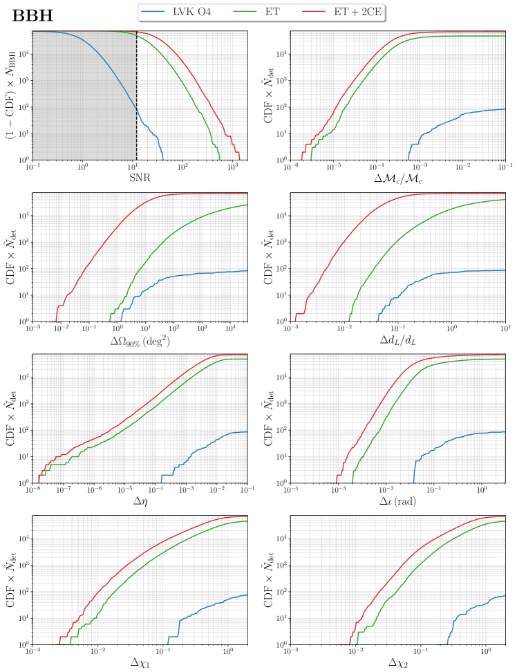
Figure 9: Cumulative distributions of the number of detections per year, for the SNRs and for the error on the parameters, for BBH signals with the three considered network configuration, using the waveform model IMRPhenomHM, and the value ${\cal R}_{0,{\rm BBH}}=$17\text{\,}{\mathrm{Gpc}}^{-3}\text{\,}{\mathrm{yr}}^{-1}$$ for the local rate. Except for the panel showing the distribution of the SNR, only the events whose Fisher matrix could be reliably inverted are included.

Another crucial information, for understanding the scientific potential of 3G detectors, is provided by the redshift distribution of the detected events, for different values of the threshold in SNR, or for different selection cuts on the accuracy that can be obtained on some especially important parameters. In the left panel of Fig. 10 we show the redshift distributions of the detected BBHs at ET alone, selected on the basis of the SNR, and we compare it to the redshift distribution of the total population. Beside showing the distribution of detected events, with detection defined from the criterion ${\rm SNR}\geq 12$, we also show the distribution in redshift of the events that satisfy a less stringent cut on the SNR, that we take for definiteness ${\rm SNR}\geq 8$, as well as the events that pass some very high thresholds on the SNR, while in the central and right panels we show the redshift distribution of the observed events (defined from the condition ${\rm SNR}\geq 12$), which furthermore pass stringent cuts on the error on the luminosity distance (central panel) or sky localization (right panel). In this figure, the upper panels give the fraction of events per redshift bin, and the lower panels give the corresponding cumulative distributions. A lower threshold on the SNR can be useful in multi–messenger observations. In general, BBHs are not expected to have an electromagnetic counterpart; however, should a counterpart be present for any of those events, the temporal association between the gravitational and electromagnetic signals could be used to lower the SNR, while maintaining a high statistically significance. Another reason for using a lower SNR, specific to ET, is that, as we have discussed in Sect. 3.1, the three–arms configuration of ET allows us to construct a null stream, where the GW signal cancels. This can provide a powerful veto against glitches and other non–Gaussian noise (Goncharov et al., 2022), that allows us to dig more confidently into events with a lower SNR. However, one must keep in mind that the Fisher matrix analysis becomes less reliable for such low values of the SNR. On the opposite side, events with very large SNR, such as ${\rm SNR}\geq 100$, or events with especially good accuracy on parameter reconstruction, are obviously interesting for precision physics, such as tests of GR or measurements of $H_{0}$. In Sect. 5.4 we will discuss these ‘golden binaries’ further. For the moment, we just observe from Fig. 10 that, with the detection criterion ${\rm SNR}\geq 12$, ET alone can detect basically $100\%$ of the population up to $z\sim 1$, and about $67\%$ of the BBH population out to $z\sim 20$; furthermore, about $1\%$ of the population up to $z\sim 10$ is detected with ${\rm SNR}\geq 100$. Fig. 11 shows the same results for the ET+2CE network. In this case, basically $100\%$ of the BBH population out to $z\simeq 2$ is detected, and $93\%$ up to $z\sim 20$. The central and right panels show the redshift distribution of events that pass the detection cut ${\rm SNR}\geq 12$, and furthermore satisfy more stringent requirement on the accuracy that can be obtained on $d_{L}$ or on sky localization. We will further comment on them in Sect. 5.4.

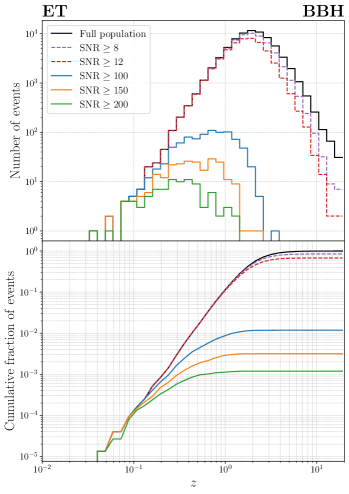
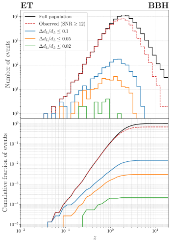
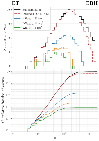
Figure 10: Redshift distributions of the BBHs observed at ET alone in 1 yr, selected on the basis of different thresholds for the SNR (left panel), or setting ${\rm SNR}\geq 12$ and applying further cuts on $\Delta d_{L}/d_{L}$ (central panel), or on $\Delta\Omega_{90\%}$ (right panel). The black solid line corresponds to the total BBH population in the astrophysical model that we have assumed. We set ${\cal R}_{0,{\rm BBH}}=$17\text{\,}{\mathrm{Gpc}}^{-3}\text{\,}{\mathrm{yr}}^{-1}$$, and show the results for the detections in one year (taking into account our assumptions of the duty cycle). In each column, the upper panel shows the number of events per redshift bin, while the lower panel shows the corresponding cumulative distributions, normalized to the number of BBH events in our sample, $N_{\rm BBH}=7.5\times 10^{4}$.

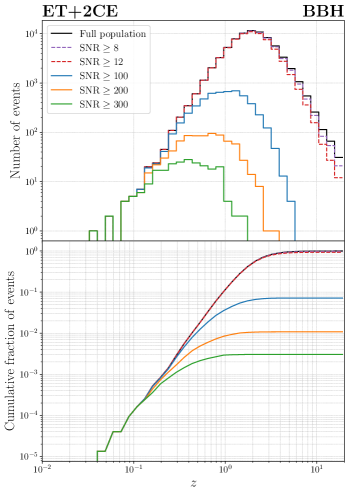
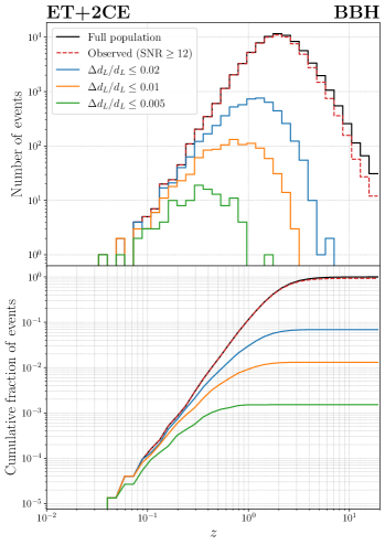
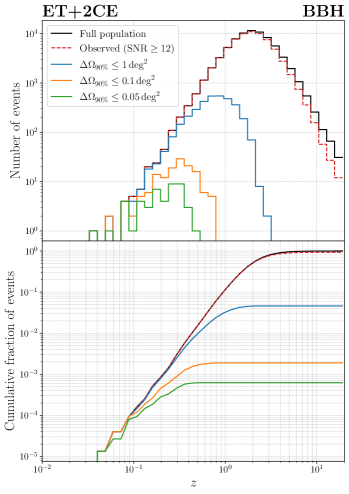
Figure 11: As in Fig. 10, for ET+2CE.

In Fig. 12 we present scatter plots showing the correlations of the errors on quantities that are relevant in cosmological and astrophysical applications of GWs. In particular, in the left panels we show the scatter of detections in the plane $(\Delta\Omega_{90\%},\,\Delta d_{L}/d_{L})$ (with a color scale giving information on the redshift). We see that, for an ET + 2CE network, about 36% of the events will have a localization region smaller than $10\text{\,}{\mathrm{deg}}^{2}$, while also having an accuracy on the luminosity distance $\Delta d_{L}/d_{L}\lesssim 10^{-1}$, even at $z\gtrsim 1$. This would have an important impact on late–time cosmology, in particular for the possibility of determining the Hubble constant and constraining the phenomenon of “modified GW propagation” (Belgacem et al., 2018a, b, 2019b) by correlating GWs and galaxy catalogs [see Finke et al. (2021); Abbott et al. (2021e); Palmese et al. (2021a) for the most recent applications]. A small fraction of the events, of order ${10}^{-3}$ (which still, for ET+2CE, and with our assumptions on the population and the local rate, corresponds to about 90 events per year), could even have a localization region $\Delta\Omega_{90\%}\lesssim${10}^{-1}\text{\,}{\mathrm{deg}}^{2}$$ and $\Delta d_{L}/d_{L}\lesssim${10}^{-2}\text{\,}$$, which could allow a unique host galaxy identification even in absence of a direct EM counterpart (Borhanian et al., 2020), either from a galaxy catalog or from a dedicated follow–up.

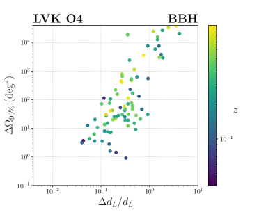
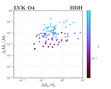
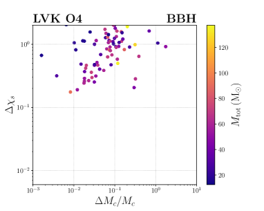
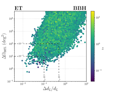
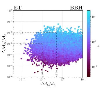
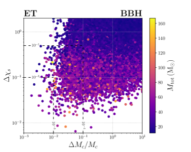
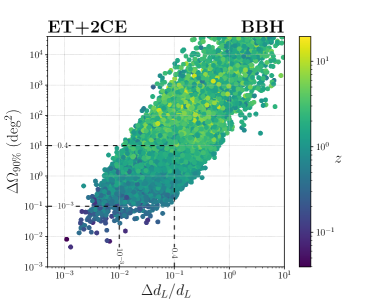
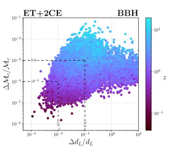
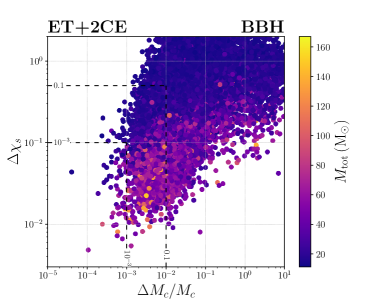
Figure 12: Scatter plots of the observed BBH population at the various networks. In the first row we show the results for the LVK network in O4, in the middle for ET alone and in the bottom for the ET + 2CE network. In each row, the left panel shows the distribution of errors on the luminosity distance and sky location, with the color code representing the redshift, the central panel the distribution of errors on the luminosity distance and detector–frame chirp mass, again with the color code representing the redshift, and the right panel the distribution of errors on the source–frame chirp mass and symmetric spin $\chi_{s}=(\chi_{1}+\chi_{2})/2$, with the color code representing the total source–frame mass. The numbers reported on the dashed lines refer to the fraction of observed events lying inside the corresponding region.

Very significant results are obtained also with ET alone, despite the limitations in the localization with a single detector, with a fraction of events of order $10^{-3}$ (which, in the case of ET alone, and with our reference value for the local rate, corresponds to about 90 events per year) having at the same time a sky localization better than $10\text{\,}{\mathrm{deg}}^{2}$ and an error on the luminosity distance $\Delta d_{L}/d_{L}\lesssim${10}^{-1}$$. As we mentioned above, ET alone will see about $10^{3}$ BBH events with $\Delta d_{L}/d_{L}\lesssim${10}^{-1}$$ and about $160$ BBH events with $\Delta\Omega_{90\%}\leq$10\text{\,}{\mathrm{deg}}^{2}$$. We see that, among these, about $90$ satisfy both criteria, $\Delta d_{L}/d_{L}\lesssim${10}^{-1}$$ and $\Delta\Omega_{90\%}\leq$10\text{\,}{\mathrm{deg}}^{2}$$, and will therefore be particularly useful for cosmological studies.

For the current network of detectors in the O4 run we find that it should observe $\sim 5$ BBHs per year with localization $\Delta\Omega_{90\%}\lesssim$10\text{\,}{\mathrm{deg}}^{2}$$ and $\Delta d_{L}/d_{L}\lesssim${10}^{-1}$$, including some sources at $z\gtrsim 0.3-0.4$. This would allow substantial improvements in the constraints on the Hubble constant within $\sim 2$ years of data taking, using the correlation with galaxy catalogs. By comparison, in the GWTC–2 and GWTC–3 catalogs, which include the detections up to the O3 run, the best localized BBH event, GW190814, has a sky localization of $19\text{\,}{\mathrm{deg}}^{2}$, and only two more BBH events, GW190412 ($21\text{\,}{\mathrm{deg}}^{2}$) and GW200208$\_$130117 ($30\text{\,}{\mathrm{deg}}^{2}$) have $\Delta\Omega_{90\%}\leq$30\text{\,}{\mathrm{deg}}^{2}$$ (Abbott et al., 2021a, b).

In the central panels of Fig. 12 we show our forecasts for the joint errors on the detector–frame chirp mass and the luminosity distance, again with a color scale giving information on the redshift. An accurate measurement of detector–frame masses, together with information on the distribution of source–frame masses, can be used to break the mass–redshift degeneracy in the GW waveform and constrain the underlying cosmological model together with the compact binary population (Farr et al., 2019; Ezquiaga, 2021; Mastrogiovanni et al., 2021b; Abbott et al., 2021e; Mancarella et al., 2022; Leyde et al., 2022; Karathanasis et al., 2022).

Finally, in the right column of Fig. 12, we show the expected errors attainable on the source–frame chirp mass and symmetric spin parameter, $\chi_{s}=(\chi_{1}+\chi_{2})/2$, with a color code that provides information on the total source–frame mass. These three parameters are of fundamental importance to characterise the astrophysical BBH population (Abbott et al., 2021c) and also to disentangle it from a possible primordial component (De Luca et al., 2020). Again, for both combinations of parameters, these results are very promising, showing the potential of the next generation of GW detectors.

For ease of readability, some selected results presented in this section are summarised in Tab. 3.

BBH
Network	Detected	Analysed	$\rm SNR\geq 100$	$\Delta d_{L}/d_{L}\leq 10\%$	$\Delta\Omega_{90\%}\leq$10\text{\,}{\mathrm{deg}}^{2}$$
LVK–O4	86	86	0	8	15
ET	50607	48456	885	1120	161
ET+2CE	69799	69610	5384	45331	30889

Table 3: A selection of results from the analysis of the $7.5\text{\times}{10}^{4}$ BBHs (corresponding to the full population in about $1\text{\,}\mathrm{yr}$ with our choices for the parameters) at the considered networks. Here, and in similar tables below, the column labeled “Analysed” reports the number of events that passed our detection threshold (${\rm SNR}\geq 12$) and for which, furthermore, we could get a reliable inversion of the Fisher matrix, according to our criterion explained in Sect. 2.2.

5.2 Binary neutron stars

We next present our results for the population of BNS systems. The current best estimates for the local merger rate, ${\cal R}_{0,\rm BNS}$, is obtained from the GWTC–3 catalog (Abbott et al., 2021c), but still suffers from a large uncertainty. Using a rather specific set of assumptions (in particular, a mass distribution for NS in binaries flat between $1$\mathrm{M_{\odot}}$$ and $2.5$\mathrm{M_{\odot}}$$), Abbott et al. (2021c) finds ${\cal R}_{0,\rm BNS}=105.5^{+190.2}_{-83.0}\leavevmode\nobreak\ ${\mathrm{Gpc}}^{-3}\text{\,}{\mathrm{yr}}^{-1}$$, consistent with the value ${\cal R}_{0,\rm BNS}=320^{+490}_{-240}\leavevmode\nobreak\ ${\mathrm{Gpc}}^{-3}\text{\,}{\mathrm{yr}}^{-1}$$ inferred from the GWTC–2 catalog using the same mass distribution (Abbott et al., 2021f), but still with a median value lower by a factor $\sim 3$. However, these numbers are quite model dependent. Three different models have been investigated in (Abbott et al., 2021c) and, taking the lowest $5\%$ and highest $95\%$ credible interval out of all three models, ${\cal R}_{0,\rm BNS}$ is inferred to be in the range $(10-1700)\leavevmode\nobreak\ ${\mathrm{Gpc}}^{-3}\text{\,}{\mathrm{yr}}^{-1}$$. In the following, we will use as reference value ${\cal R}_{0,\rm BNS}=$105.5\text{\,}{\mathrm{Gpc}}^{-3}\text{\,}{\mathrm{yr}}^{-1}$$, which is the median value obtained for the flat mass distribution that we are using, but it is important to keep in mind the uncertainty on this number, which could be up to a factor $\sim 10$ lower, or up to a factor $\sim 16$ higher. We then simulate a population of $N_{\rm BNS}=${10}^{5}$$ BNS out to $z=20$, which, for ${\cal R}_{0,\rm BNS}=$105.5\text{\,}{\mathrm{Gpc}}^{-3}\text{\,}{\mathrm{yr}}^{-1}$$, and our assumed redshift dependence for the merger rate, corresponds to the number of coalescences in about one year.

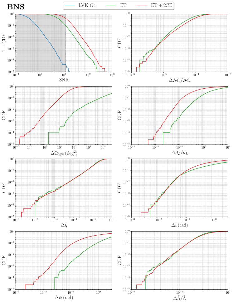
Figure 13: Cumulative distributions of the event fraction for BNS signals as function of SNR (for LVK–O4, ET and ET+2CE) and as a function of parameter errors (for ET and ET+2CE), using the waveform model IMRPhenomD_NRTidalv2.

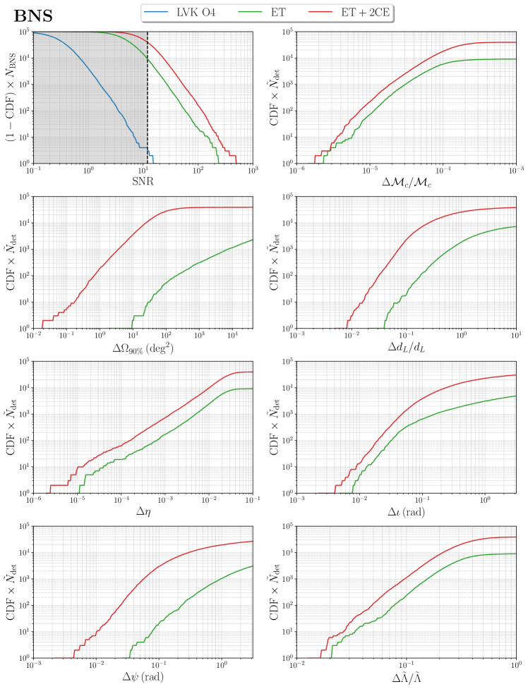
Figure 14: As in Fig. 13, in terms of the total number of events rather than detection fraction, using ${\cal R}_{0,\rm BNS}=105.5\,{\rm Gpc}^{-3}{\rm yr}^{-1}$. Except for the panel showing the distribution of the SNR, only the events whose Fisher matrix could be reliably inverted are included.

For this value of the local rate, for the current LVK network of detectors during the O4 run and accounting for the duty cycle, we find that only about 4 events per year should detected, consistently with the forecast in Abbott et al. (2020b). Even assuming the current detectors to be operational 100% of the time during O4, the number of detections just raises to 5. Given the smallness of this sample, for LVK–O4 we do not plot the results for the parameter estimation of the corresponding events, since they would strongly depend on the particular random realization considered. Therefore, except for the cumulative distribution of the SNR, we only show the results for ET and for ET+2CE.

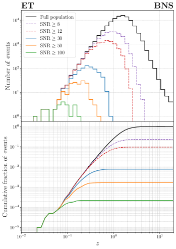
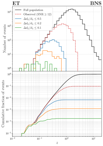
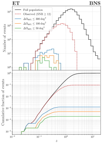
Figure 15: Redshift distributions of the BNSs observed at ET alone, selected on the basis of different thresholds for the SNR (left panel), or setting ${\rm SNR}\geq 12$ and applying further cuts on $\Delta d_{L}/d_{L}$ (central panel), or on $\Delta\Omega_{90\%}$ (right panel). The black solid line corresponds to the total BNS population in the astrophysical model that we have assumed. We set ${\cal R}_{0,{\rm BNS}}=$105.5\text{\,}{\mathrm{Gpc}}^{-3}\text{\,}{\mathrm{yr}}^{-1}$$, and show the results for the detections in one year (taking into account our assumptions of the duty cycle). Given the uncertainly on ${\cal R}_{0,{\rm BNS}}$, which currently can be in the range $(10-1700)\leavevmode\nobreak\ ${\mathrm{Gpc}}^{-3}\text{\,}{\mathrm{yr}}^{-1}$$, one should keep in mind that the absolute number can still change by a factor $\order{10}$ or more. In each column, the upper panel shows the number of events per redshift bin, while the lower panel shows the corresponding cumulative distributions, normalized to the number of BNS events in our sample, $N_{\rm BNS}=${10}^{5}$$.

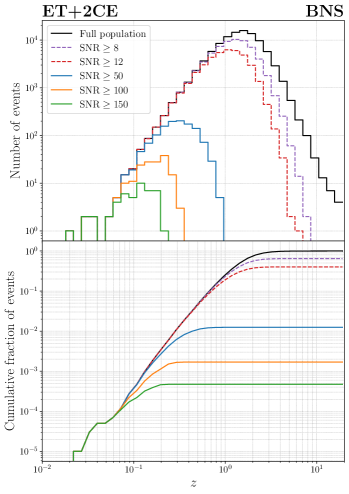
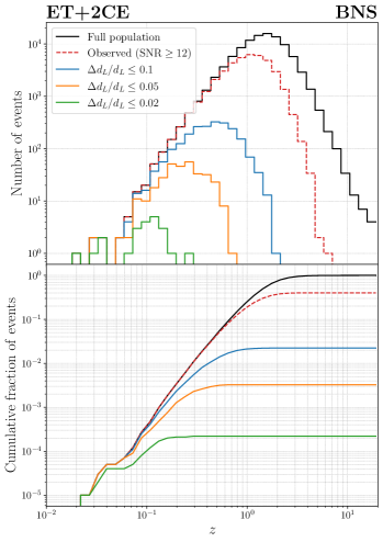
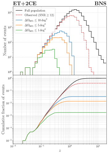
Figure 16: As in Fig. 15, for ET+2CE.

For 3G detectors, with our threshold ${\rm SNR}\geq 12$ we find $N_{\rm det}\simeq$9.6\text{\times}{10}^{3}$$ detections per year for ET alone (corresponding to $9.6\%$ of the population) and $N_{\rm det}\simeq$4.0\text{\times}{10}^{4}$$ detections per year for ET + 2CE (corresponding to $40.1\%$ of the population). Varying ${\cal R}_{0,\rm BNS}$ in the currently allowed range $(10-1700)\,{\rm Gpc}^{-3}{\rm yr}^{-1}$, while keeping fixed the redshift distribution of our population model, the number of detections per year at LVK–O4 ranges between zero and 65, for ET varies in the range $[$9.1\text{\times}{10}^{2}$,$1.6\text{\times}{10}^{5}$]$, and for ET+2CE varies in the range $[$3.8\text{\times}{10}^{3}$,$6.5\text{\times}{10}^{5}$]$. When performing parameter estimation, we will restrict again to the $\tilde{N}_{\rm det}$ detected events that also pass our criterion for having a reliable inversion of the Fisher matrix. We find $\tilde{N}_{\rm det}\simeq$9.2\text{\times}{10}^{3}$$ for ET (corresponding to about $96\%$ of the detected events), and $\tilde{N}_{\rm det}\simeq$4.0\text{\times}{10}^{4}$$ (corresponding to about $99\%$ of the detected events) for ET+2CE.

Our results for the SNR and for parameter estimation are shown in Fig. 13 (where we show the detection fractions) and in Fig. 14 (where, for parameter estimation, we multiply the detection fractions at the different detector networks by the respective values of $\tilde{N}_{\rm det}$, and for the SNR we multiply by $N_{\rm BNS}$), while in Fig. 15 we show the redshift dependence of various distributions at ET, similarly to Fig. 10 for the BBH case; in Fig. 16 we show the corresponding results for ET+2CE.

Compared to BBHs, the smaller mass of BNSs allows them to stay longer in the detector band, but makes them less loud, thus more difficult to see, especially at high redshifts. As we discussed in Sect. 3.2, thanks to the long time spent in the detector bandwidth at ET, the BNS localization can be improved by exploiting the rotation of the Earth. From the panel for $\Delta\Omega_{90\%}$ in Fig. 13 and 14 we see that, for BNS, with our fiducial values of the rate and our assumptions on the population, ET as a single detector can reach an error of order $10\,${\mathrm{deg}}^{2}$$ for the very best localized sources, and about $0.6\%$ of the detected BNS will have $\Delta\Omega_{90\%}<${10}^{2}\text{\,}{\mathrm{deg}}^{2}$$. When comparing with other results in the literature, it is important to observe that, given the current large uncertainty on the BNS local rate and population properties, different papers can use very different assumptions, which can easily lead to results differing by about one order of magnitude. In particular, in App. B we compare with the results found in Borhanian & Sathyaprakash (2022) and in Ronchini et al. (2022), where we find that our results are consistent, once the differences in the assumptions made (all legitimate, within the current uncertainties), are taken into account.

It is interesting to observe that, despite the improvement brought by the inclusion of the Earth’s rotation (which is only relevant for BNSs, given the long duration of their signal) still, for ET as a single detector, the localization accuracy of BNSs is not comparable to that of BBHs, that was shown in the corresponding panel of Fig. 9. For instance, with a single ET detector a fraction of about $3\text{\times}{10}^{-3}$ of the detections (corresponding, for our fiducial value of the local rate and our population model, to $\order{150}$ BBH/yr) can be localized to better than $10\text{\,}{\mathrm{deg}}^{2}$, while, with our assumptions on the BNS local rate and BNS population model, we only find 2 BNS that can be localized to such an accuracy. This shows that the loudness of typical BBH signals is more important, for sky localization, than the long time spent in the bandwidth by BNS signals.

For a network ET+2CE, thanks to triangulation, we see again from Fig. 14 that we can reach an accuracy below ${10}^{-1}\text{\,}{\mathrm{deg}}^{2}$ for the best localized BNS systems, to be compared with the localization below ${10}^{-2}\text{\,}{\mathrm{deg}}^{2}$ that ET+2CE can reach for the best localized BBHs, as we saw in Fig. 9. However, it is important to notice that, for multi–messenger observations of BNSs and for the identification and follow–up of the associated kilonova, already the angular resolution of a single ET detector can be adequate. For instance, to understand the nucleosynthesis spectra of the kilonova, for sources up to $z\simeq 0.3-0.4$ the best instrument is the Extremely Large Telescope (ELT),. However, a direct pointing with ELT would require arcsec localization, which is anyhow out of question for GW detectors. The actual, strategy for sources at these moderate redshifts, is rather to use telescopes with large field–of–view (FOV): these instruments, with a localization of the GW events of the order of tens to hundreds of square degrees, can indeed localize the source. Notice that such a GW resolution can be given already by ET alone. In particular, the Vera Rubin Observatory’s LSST (Ivezić et al., 2019) has a FOV of $9.6\text{\,}{\mathrm{deg}}^{2}$ and can observe kilonovae up to $z\sim 0.1$ (with $5\%$ of the kilonovae observable up to $z\simeq 0.4$) and several other instruments, such as ULTRASAT (Sagiv et al., 2014), can reach $z\simeq 0.1$; the Nancy Roman Space Telescope (formerly WFIRST) (Spergel et al., 2015) has the highest reach, being able to observe $50\%$ of the kilonovae up to $z\sim 0.2-0.3$, with $5\%$ of the kilonovae observable up to $z\simeq 1$, although its FOV, $0.28\text{\,}{\mathrm{deg}}^{2}$, is not as large, so it requires sub–degree localization, or an earlier localization by instruments with a larger FOV (see Cowperthwaite et al. (2019); Chase et al. (2022); Ronchini et al. (2022) for recent discussions). Once localized the kilonova with these large FOV instruments, telescopes such as the ELT can perform a more detailed follow–up of the source. For BNSs at larger redshifts, the identification of the electromagnetic counterpart can only be made by ${\rm X}/\gamma$–ray satellites with large FOV; a sky localization of order $100\text{\,}{\mathrm{deg}}^{2}$, as can be provided by ET alone, is about $1/10$ of the typical FOV of wide–field X–ray telescope, which in general is larger than $1\text{\,}\mathrm{sr}$, so such a localization can already provide sufficient information for the search and localization of the $\gamma$– or X–ray counterpart; then, the ${\rm X}/\gamma$–ray satellites can provide the arcmin localization needed to drive the ground–based follow–up (Ronchini et al., 2022). For these multi–messenger studies, a lower threshold on the SNR, such as ${\rm SNR}=8$, can be appropriate, since the statistical significance will be enhanced by the temporal coincidence of the gravitational and electromagnetic signals. From the upper–left panel of Fig. 15 we see that, for ET alone and a threshold ${\rm SNR}=8$, the farthest detected BNSs in our sample are at $z\sim 4.5$ (the farthest one happens to be at $z\simeq 4.77$ and has $M_{\rm tot}=$4.15\text{\,}\mathrm{M_{\odot}}$$ and nearly equal masses). Higher values of the rate, or longer observation times, would lead to the gradual appearance of more and more rare events. For ${\rm SNR}=8$, at ET alone, an equal mass non–spinning BNS, with $m_{1}=m_{2}=$1.35\text{\,}$Msun{\mathrm{M_{\odot}}}$$$, optimal inclination and sky location could be detected up to $z_{\rm max}\simeq 3.5$, while a heavier equal mass non–spinning BNS, say with $m_{1}=m_{2}=$2.1\text{\,}$Msun{\mathrm{M_{\odot}}}$$$, optimal inclination and sky location could be detected up to $z_{\rm max}\simeq 6.9$. These estimates are in agreement with those in Ronchini et al. (2022). For ET+2CE, the farthest detection in our sample, with ${\rm SNR}\geq 8$, is at $z\simeq 8.8$ and has $M_{\rm tot}=$3.73\text{\,}\mathrm{M_{\odot}}$$ and a mass ratio of $q\simeq 1.33$. An ideally oriented BNS with the same (rather extreme) characteristics could in principle be detected up to $z\simeq 20$ (where, of course, NSs are not even expected to exist), while a more realistic equal–mass non–spinning BNS, with $m_{1}=m_{2}=$1.35\text{\,}$Msun{\mathrm{M_{\odot}}}$$$, could be detected up to $z\simeq 11$.

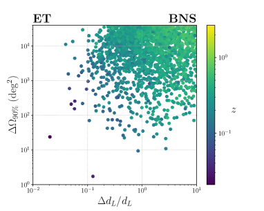
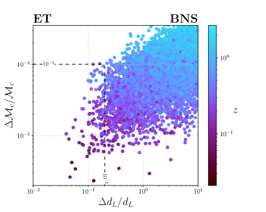
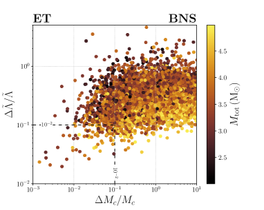
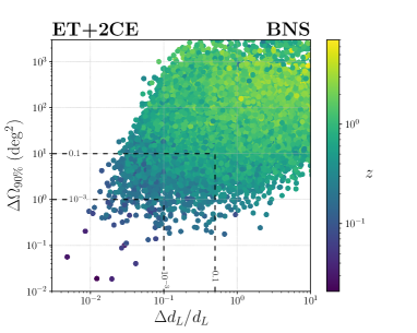
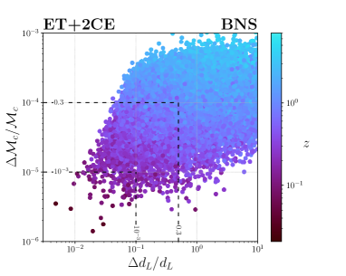
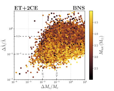
Figure 17: Scatter plots of the observed BNS population at 3G detectors. On the top row we report the results for ET alone and in the bottom for the ET + 2CE network. In each row, the left panel shows the distribution of errors on the luminosity distance and sky location as a function of redhsift, the central panel the distribution of errors on the luminosity distance and detector–frame chirp mass as a function of redshift, and the right panel the distribution of errors on the source–frame chirp mass and adimensional tidal deformability as a function of the total source–frame mass. The numbers reported on the dashed lines refer to the fraction of observed events lying inside the corresponding region.

When drawing conclusions from plots featuring the absolute number of BNS detections, it is important to keep in mind that the estimate of ${\cal R}_{0,{\rm BNS}}$ from current observations is still very uncertain, given the limited sample of detected BNS coalescences, much more than for BBHs, for which we already have a much larger sample of detections. As we have mentioned above, current data, depending on the model used (e.g. on the assumed mass, spin and redshift distributions) are consistent with values of ${\cal R}_{0,{\rm BNS}}$ in the range $(10-1700)\leavevmode\nobreak\ ${\mathrm{Gpc}}^{-3}\text{\,}{\mathrm{yr}}^{-1}$$. Therefore, as more and more BNS detections will accumulate with future runs, and the BNS local rate will become better constrained, the absolute scale on the vertical axis in Fig. 14 could still change, possibly by as much as a factor $\order{10}$. Furthermore, a change in the rate is not just reabsorbed in a rescaling of the absolute vertical scale of these plots. For a fixed observation time, such as the standard reference choice of one year, the tails of the distributions, i.e. rare and particularly interesting events, change. As an obvious example, if, with a given choice of rate, in one year there is no event with, say, $z>4$, this does not mean that, with a rate three times larger, there will be three times zero events, which is still zero. Rarer and rarer events will appear as we increase the rate or the observation time. Therefore, given the current large uncertainty, when comparing different results for BNSs in the literature, one must first of all check the value of ${\cal R}_{0,{\rm BNS}}$ used.

Finally, similarly to the plots shown for BBH signals, in the left and central panels of Fig. 17 we show scatter plots of the joint estimation errors for the sky location and luminosity distance, and for detector–frame chirp mass and luminosity distance, with a color code showing the redshift dependence. These are again the basis for the statistical methods based on correlation with galaxy catalogs and the mass function, the latter being particularly promising given the expected narrowness of the BNS mass distribution (Taylor et al., 2012; Finke et al., 2022). Exploiting statistical techniques is of fundamental importance also for BNS systems even though they can have an associated electromagnetic counterpart, since the detection of such EM emissions is expected only for a fraction of the sources (Belgacem et al., 2019a; Ronchini et al., 2022). In the right panels of Fig. 17 we instead report the forecast of the relative errors attainable on the source–frame chirp mass and the combination of the adimensional tidal deformability parameters $\tilde{\Lambda}$ defined in Eq. (14) (with a color code giving information on the total source–frame mass). These are the basic quantities needed to study the equation of state of dense matter above the nuclear density. We find a large amount of detections with percent–level accuracy attainable both at ET alone and at ET+ 2CE detectors. This would lead to dramatic improvements in our understanding of the equation of state of NSs [see e.g. Gupta et al. (2022) for a recent discussion]. We again show a selection of some of the main results presented in this section in Tab. 4.

BNS
Network	Detected	Analysed	$\rm SNR\geq 30$	$\Delta d_{L}/d_{L}\leq 10\%$	$\Delta\Omega_{90\%}\leq$100\text{\,}{\mathrm{deg}}^{2}$$
LVK–O4	4	4	0	1	2
ET	9577	9153	770	18	51
ET+2CE	40107	39584	5289	2225	27331

Table 4: A selection of results from the analysis of the $1\text{\times}{10}^{5}$ BNSs (corresponding to the full population in about $1\text{\,}\mathrm{yr}$ with our choices for the parameters) at the considered networks.

5.3 Neutron star–black hole binaries

Finally, we present our results for the population of NSBH systems, for which, currently, there are only two detections, which took place in the second part of the O3 run. In Abbott et al. (2021g), the local rate has been estimated to be ${\cal R}_{0,{\rm NSBH}}=45^{+75}_{-33}\leavevmode\nobreak\ ${\mathrm{Gpc}}^{-3}\text{\,}{\mathrm{yr}}^{-1}$$ (assuming that the observed NSBH are representative of the underlying population), or ${\cal R}_{0,{\rm NSBH}}=130^{+112}_{-69}\leavevmode\nobreak\ ${\mathrm{Gpc}}^{-3}\text{\,}{\mathrm{yr}}^{-1}$$ (assuming a broad NSBH population), while the re–analysis in Abbott et al. (2021c), using different modelizations, produce broadly consistent rates, between $7.8$ and $140\text{\,}{\mathrm{Gpc}}^{-3}\text{\,}{\mathrm{yr}}^{-1}$. In the following, as a reference value, we will assume for definiteness the value ${\cal R}_{0,{\rm NSBH}}=$45\text{\,}{\mathrm{Gpc}}^{-3}\text{\,}{\mathrm{yr}}^{-1}$$, keeping in mind that the current uncertainty on the local rate can result in an increase or a decrease in the number of detections per year, by a factor $\sim 3$ in either direction.

For these systems, we then simulate a population of $N_{\rm NSBH}=$4.5\text{\times}{10}^{4}$$ sources out to $z=20$ that, with our reference value of ${\cal R}_{0,{\rm NSBH}}$ and the redshift dependence of the merger rate that we have assumed, described in Sect. 4.1, would correspond to the number of coalescences happening in about one year. The cumulative distributions for the SNRs and for the parameter errors are shown in Fig. 18 and 19, for the relative fractions and the absolute number of detection, respectively, while the redshift distributions are shown in Fig. 20 for ET and in Fig. 21 for ET+2CE. We find that, at ${\rm SNR}\geq 12$, ET alone can detect up to $24\%$ of the sources (corresponding, with our assumptions on the population, to about $1.1\text{\times}{10}^{4}$ detections per year), while a network consisting of ET + 2CE could be able to detect 66% of the full population of sources (corresponding to about $3.0\text{\times}{10}^{4}$ detections per year). In contrast, for the current network of detectors during O4, accounting for the duty cycle, we get 3 events, again in agreement with the broad expectations of Abbott et al. (2020b). Assuming the current detectors to be operational 100% of the time during O4 the number of detections only raises to 4, thus again we do not plot the corresponding results for the parameter estimation. Varying ${\cal R}_{0,\rm NSBH}$ in the currently allowed range $(7.8-140)\leavevmode\nobreak\ ${\mathrm{Gpc}}^{-3}\text{\,}{\mathrm{yr}}^{-1}$$ (while keeping fixed the redshift dependence of the merger rate and the other features of our population model), the number of detection per year at LVK–O4 ranges between one and 10, for ET varies in the range $[$1.9\text{\times}{10}^{3}$,$3.4\text{\times}{10}^{4}$]$ and, for ET+2CE, varies in the range $[$5.2\text{\times}{10}^{3}$,$9.2\text{\times}{10}^{4}$]$. For parameter estimation, using ${\cal R}_{0,{\rm NSBH}}=$45\text{\,}{\mathrm{Gpc}}^{-3}\text{\,}{\mathrm{yr}}^{-1}$$, the corresponding values of $\tilde{N}_{\rm det}$ are $9.4\text{\times}{10}^{3}$ for ET ($87\%$ of the detected events) and $2.9\text{\times}{10}^{4}$ for ET+2CE ($99\%$).

In Fig. 22 we show scatter plots for some combinations of parameters. In particular, in the left and central panels we show the scatter plots in the $(\Delta\Omega_{90\%},\Delta d_{L}/d_{L})$ plane and in the $(\Delta{\cal M}_{c}/{\cal M}_{c},\Delta d_{L}/d_{L})$ plane, respectively, with a color code carrying information on the redshift. Also in the case of NSBHs, these quantities are relevant when exploiting statistical techniques to extract cosmological and astrophysical information from GWs. NSBH systems could be particularly relevant for probing the so–called lower mass gap, whose identification would have significant implications (Ezquiaga & Holz, 2022). For this reason, in the right panels we show the relative errors in the reconstruction of the source–frame chirp mass and symmetric mass ratio as a function of the total source–frame mass. These parameters are in fact fundamental to identify the edges of the lower mass gap, as well as identifying the system.

The knowledge that we currently have on the distribution of NSBH systems is quite limited. The large uncertainties characterising the astrophysical properties of the NSBH population are apparent looking, e.g., at Fig. 14 in Broekgaarden et al. (2021), where the authors compare the results for 420 different models, and already the shapes of the resulting distributions can be significantly different. We thus find useful to study how our results for this class of sources change with different assumptions. In our fiducial NSBH model, discussed in Sect. 4.1, the BH mass distribution is relatively narrow, and we assumed a time delay distribution $P(t_{d})\propto 1/t_{d}$, which favours small time delays. We compare it with two of the models presented in Broekgaarden et al. (2021): their fiducial model, characterised by a broader distribution for the BH mass and a time delay distribution favouring higher values, and the model denoted by O_111, which predicts smaller masses and low time delays. These can be seen, respectively, as an “optimistic” and a “pessimistic” scenario, since systems with higher masses and closer to the observer are louder and easier to detect. Observe that even more optimistic or pessimistic scenarios are possible, see e.g. Santoliquido et al. (2021b).

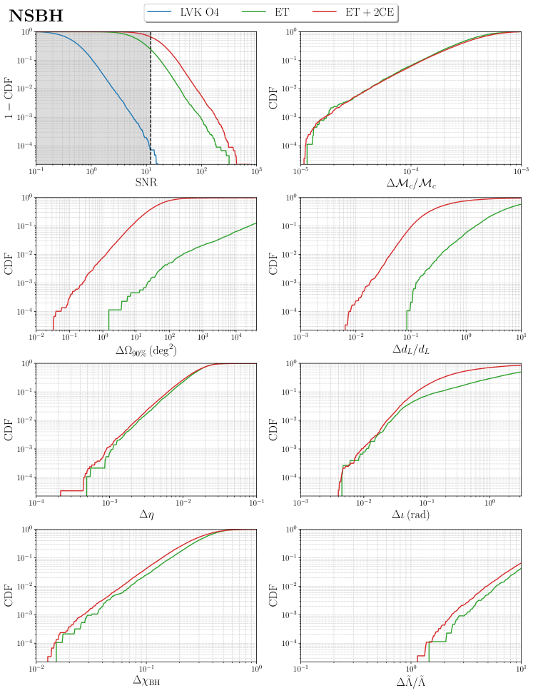
Figure 18: Cumulative distributions of the SNRs (for LVK–O4, ET and ET+2CE) and parameter errors (for ET and ET+2CE) for NSBH signals, using the waveform model IMRPhenomNSBH.

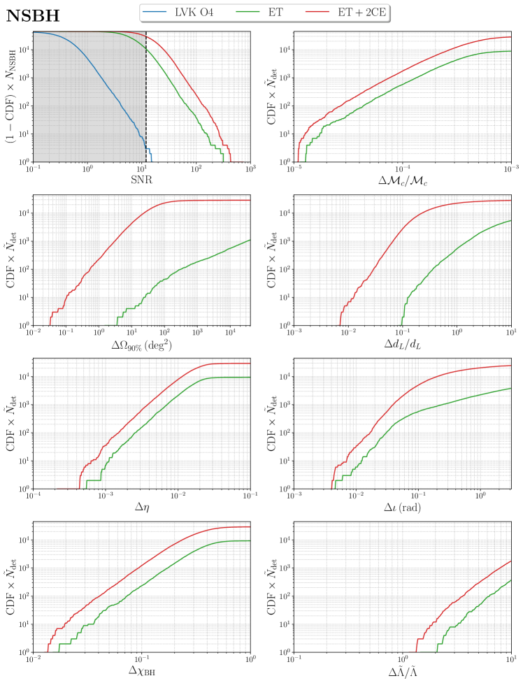
Figure 19: As in Fig. 18, in terms of the total number of events rather than detection fraction.

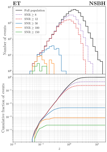
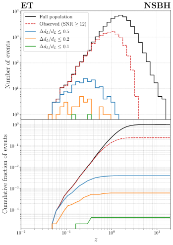
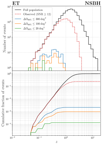
Figure 20: Redshift distributions of the NSBHs observed at ET alone, selected on the basis of different thresholds for the SNR (left panel), or setting ${\rm SNR}\geq 12$ and applying further cuts on $\Delta d_{L}/d_{L}$ (central panel), or on $\Delta\Omega_{90\%}$ (right panel). The black solid line corresponds to the total NSBH population in the astrophysical model that we have assumed. We set ${\cal R}_{0,{\rm NSBH}}=$45\text{\,}{\mathrm{Gpc}}^{-3}\text{\,}{\mathrm{yr}}^{-1}$$, and show the results for the detections in one year (taking into account our assumptions of the duty cycle). Given the current uncertainly on ${\cal R}_{0,{\rm NSBH}}$, one should keep in mind that the absolute number can still change by a factor $\order{3}$. In each column, the upper panel shows the number of events per redshift bin, while the lower panel shows the corresponding cumulative distributions, normalized to the number of BNS events in our sample, $N_{\rm NSBH}=$4.5\text{\times}{10}^{4}$$.

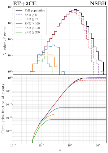
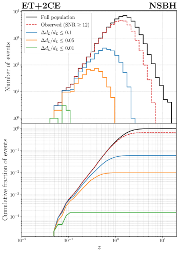
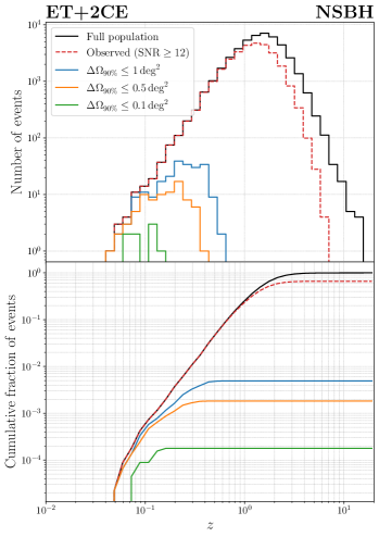
Figure 21: As in Fig. 20, for ET+2CE.

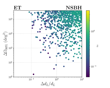
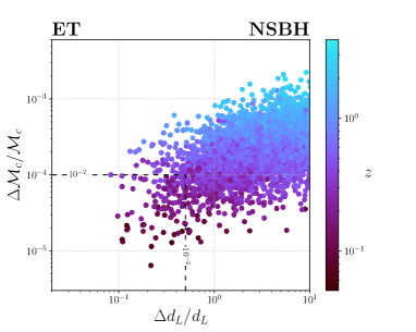
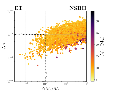
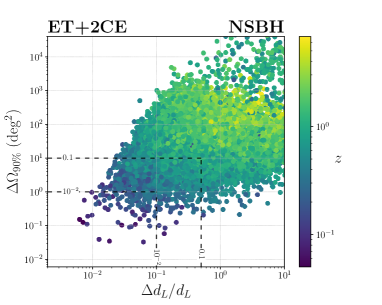
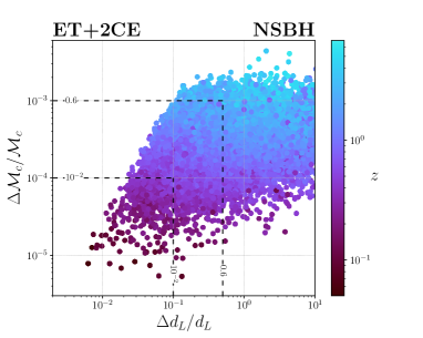
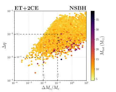
Figure 22: Scatter plots of the observed NSBH population at 3G detectors. On the top row we report the results for ET alone and in the bottom for the ET + 2CE network. In each row, the left panel shows the distribution of errors on the luminosity distance and sky location as a function of redhsift, the central panel the distribution of errors on the luminosity distance and detector–frame chirp mass as a function of redhsift, and the right panel the distribution of errors on the source–frame chirp mass and symmetric mass ratio as a function of the total source–frame mass. The numbers reported on the dashed lines refer to the fraction of observed events lying inside the corresponding region.

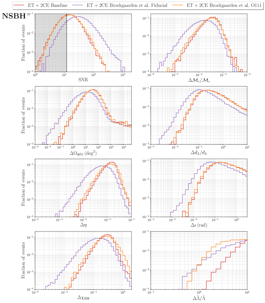
Figure 23: Histograms of the parameter errors for NSBHs with the ET+2CE network configuration, using the waveform model IMRPhenomNSBH, and sampling the BH mass and system redshift from our baseline distribution, and from two distributions taken from (Broekgaarden et al., 2021). The tails of the distributions featuring extremely large values of the relative errors, as in some of the panels, simply represents the contribution of events for which the Fisher matrix approximation cannot be trusted.

To perform the comparison, we fitted the quantiles of the chosen distributions provided in Broekgaarden et al. (2021), with suitable metalog distributions (Keelin, 2016), capable of reproducing PDFs with irregular features. The comparison is only made using the ET + 2CE detector network, which has the highest number of detections, in order to avoid a proliferation of plots and for ease of readability. We show the results in Fig. 23, from which it is apparent that the uncertainties characterising the distribution of these events can strongly impact our results. In particular, as expected, the parameter errors for the events characterised by the narrower rate distribution can be much lower, even by more than one order of magnitude, as compared to the results obtained with our baseline choices, which, in contrast, are in good agreement with the broader distribution. Furthermore, also the SNRs obtained for the “optimistic” population are on average much higher, resulting in an increased percentage of detections, from $66\%$ to $89\%$, while the percentage of detections in the “pessimistic” case remains consistent with our fiducial choices. The results on NSBHs shown in this work could thus change significantly in the future, when the population of NSBH systems will be better explored, and should only be considered as a first step toward understanding the capabilities of GW detectors for NSBH systems, although our estimates appear to be more on the conservative side. Also in this case we summarise some of the main results presented in this section in Tab. 5.

NSBH
Network	Detected	Analysed	$\rm SNR\geq 50$	$\Delta d_{L}/d_{L}\leq 10\%$	$\Delta\Omega_{90\%}\leq$100\text{\,}{\mathrm{deg}}^{2}$$
LVK–O4	3	3	0	0	1
ET	10792	9384	223	2	44
ET+2CE	29707	29462	1785	2687	22821

Table 5: A selection of results from the analysis of the $4.5\text{\times}{10}^{4}$ NSBHs (corresponding to the full population in about $1\text{\,}\mathrm{yr}$ with our choices for the parameters) at the considered networks.

5.4 ‘Golden binaries’ at 3G detectors

The detection rate of compact binaries at 3G detectors is huge. As we have seen, for BBHs (keeping fixed the redshift dependence of the merger rate and varying only the local rate) the number of detections per year should be in the range $[$3.1\text{\times}{10}^{4}$,$8.0\text{\times}{10}^{4}$]$ at ET, raising to $[$4.2\text{\times}{10}^{4}$,$1.1\text{\times}{10}^{5}$]$ for ET+2CE. Similarly, for BNSs, again keeping fixed the redshift dependence of the merger rate and varying only the local rate, the number of detections per year are expected to be in the range $[$9.1\text{\times}{10}^{2}$,$1.6\text{\times}{10}^{5}$]$ for ET, and $[$3.8\text{\times}{10}^{3}$,$6.5\text{\times}{10}^{5}$]$ for ET+2CE, and even larger numbers can be obtained with different models for the redshift dependence of the merger rate, as we discuss in App. B. For NSBHs the detections should be of order $[$1.9\text{\times}{10}^{3}$,$3.4\text{\times}{10}^{4}$]$ for ET and $[$5.2\text{\times}{10}^{3}$,$9.2\text{\times}{10}^{4}$]$ for ET+2CE.

These numbers are remarkable, and constitute one of the strength of 3G detectors. However, such large rates pose new challenges, compared to the situations at 2G detectors. For instance, a detection rate of $$5\text{\times}{10}^{3}$\,{\rm BNS/yr}$ corresponds to about a BNS every $2\text{\,}\mathrm{hr}$, while a detection rate of $8\text{\times}{10}^{4}$ BNS/yr means about one every $7\text{\,}\mathrm{min}$. As we already mentioned, BNSs can stay in the bandwidth of 3G detectors for hours, or up to order one day. This means that we will have to deal with overlapping signals, as has been recognized already since several years (Regimbau & Hughes, 2009; Regimbau et al., 2012; Meacher et al., 2016; Regimbau et al., 2017). In particular, in Samajdar et al. (2021), assuming values of the BBH local rate in the range $[15,37.9]\leavevmode\nobreak\ ${\mathrm{Gpc}}^{-3}\text{\,}{\mathrm{yr}}^{-1}$$ and BNS local rates in the range $[80,810]\leavevmode\nobreak\ ${\mathrm{Gpc}}^{-3}\text{\,}{\mathrm{yr}}^{-1}$$, consistent with the range of values that we have used, it is found that, at a network ET+2CE, a BNS signal will typically have tens of overlapping BBH and BNS signals, and it will happen up to $\order{10^{4}}$ times per year that two signals enters their final merger phase within seconds of each other (see also Himemoto et al. (2021) for similar estimates). The bias that the overlap of signals can introduce in the parameter reconstruction of each separate event has been studied recently in Samajdar et al. (2021); Pizzati et al. (2022); Himemoto et al. (2021); Antonelli et al. (2021); these works show that the overlap of signals can indeed introduce a bias in parameter reconstruction, when two signals with comparable SNR have a difference in merger times which is no longer large compared to the accuracy to which merger times themselves can be measured.

Beside problems related to the overlap of signals, another practical problem related to the huge number of detections expected at 3G detectors is that the computation of the full multi–dimensional posteriors of such a large number of events might be computationally too expensive (see Smith et al. (2021) for recent progress in this direction).

For some scientific questions, a possible solution to these problems, which might be sub–optimal but has the advantage of simplicity, is to restrict to events with a very large SNR, say ${\rm SNR}\geq 100$; we will refer to them as ‘golden events’, or ‘golden binaries’. For some aspects of the science at 3G detectors such a strategy might have limited value. For instance, for populations studies, the completeness of the sample of detections is a key element. However, for precision studies, such as tests of General Relativity or cosmological observations, the result can be largely dominated by the very best events. For instance, in order to test gravity near the BH horizons and to discriminate the BH solution of General Relativity from other possible types of compact objects (see Cardoso et al. (2016) for general discussion) one needs events with a sufficiently large SNR in the ringdown phase, which would allow the extraction of the frequency and damping time of at least two different quasi–normal modes, allowing us to perform ‘BH spectroscopy’ (Berti et al., 2016). For this kind of questions, only events with a sufficiently large SNR are relevant. The same can happen in cosmological studies that make use of ‘dark sirens’, i.e. coalescing binaries without an observed electromagnetic counterpart, by correlating them with galaxy catalogs. In this case, the results that can be obtained for $H_{0}$, or for the parameter $\Xi_{0}$ that characterizes modified GW propagation (Belgacem et al., 2018a, b), is largely dominated by the events with the smallest localization volume, that fall in a region where a galaxy catalog is sufficiently complete, see Finke et al. (2021). Another example is provided by multi–messenger observations; given a BNS detection rate of order one event per hour or more, only for a small fraction of detections it will be conceivable to perform a dedicated follow–up by electromagnetic observations.

In all these cases, for each redshift range of interest, it will be natural to focus on the best characterized GW events. Generically, these are the ones with the highest SNR although, depending on the application that one has in mind, one might wish to perform the cut by selecting directly the events with $\Delta d_{L}/d_{L}$ below a given value, or with an angular resolution below a given value (of course, these choices are correlated, as we also see from the scatter plots in Fig. 12). It is therefore interesting to discuss in more detail the ensemble of detections with large SNR, or with small error on distance, or with good angular resolution, that we generically call ‘golden binaries’. In the left panel of Fig. 10 we showed the distribution in redshift of BBHs at ET alone, for different cuts on the SNR, including very high thresholds (${\rm SNR}\geq 100$, ${\rm SNR}\geq 150$ and ${\rm SNR}\geq 200$), while in the central panel we considered the events detected, according to the criterion ${\rm SNR}>12$, and we imposed further cuts based on $\Delta d_{L}/d_{L}$, or (in the right panel), based on $\Delta\Omega_{90\%}$; Fig. 11 showed the same result for BBH at ET+2CE. These plots show the number of events obtained in one year, for our reference value ${\cal R}_{0,{\rm BBH}}=$17\text{\,}{\mathrm{Gpc}}^{-3}\text{\,}{\mathrm{yr}}^{-1}$$ of the local BBH rate, taking into account the duty cycle, computed according to the assumptions in Sect. 4.2. As we already mentioned, it is important to keep in mind that, since we are looking for events in the tails of the distributions (whether with respect to SNR, $\Delta d_{L}/d_{L}$, or $\Delta\Omega_{90\%}$), changes in the rate, or in the observation time, or in the duty cycle, can have significant effects. In particular, increasing one or the other, will in general lead to the appearance of rarer events, i.e. events with larger SNR, better distance measurements, and/or better angular localization.

From Fig. 10, or from Tab. 3, we can appreciate that, already at ET alone (with our fiducial choices for the local rate, the redshift dependence of the merger rate, and the BBH mass function) there will be $\order{800}$ BBH detections per year with ${\rm SNR}\geq 100$, of which a significant fraction is at $z\gtrsim 1$, and a few of them are even at redshifts as large as $z\sim 3-4$; in our sample realization, the farthest event with ${\rm SNR}\geq 100$ has $z\simeq 3.8$. In terms of accuracy on distance, there are $\order{${10}^{3}$}$ events/yr with $\Delta d_{L}/d_{L}<0.1$, of which a large fraction is at $z>1$; furthermore, there are $\order{200}$ events/yr with $d_{L}$ measured to better than $5\%$, again with a large fraction of them at $z>1$.

For ET+2CE, we see from Fig. 11 or Tab. 3 that these numbers raise by almost one order of magnitude. There are now $\order{5000}$ events/yr with ${\rm SNR}\geq 100$, of which $\order{150}$ events/yr have $z\gtrsim 3$. For the luminosity distance, we find $\order{1000}$ events/yr with $d_{L}$ measured better than $1\%$; again a significant fraction of them is at $z>1$, and, out of them, $\order{40}$ events/yr are at redshifts as large as $z\sim 2-3$. Thanks to triangulation, now also for the angular resolution we have remarkable results: there are $\order{1200}$ events/yr at $z\gtrsim 1$ localized to better than $1\text{\,}{\mathrm{deg}}^{2}$, and tens of events, still at cosmologically significant redshifts, localized to better than $0.05\text{\,}{\mathrm{deg}}^{2}$. An especially remarkable result is that about 4 BBH systems per year at ET+2CE could be localised in a region as small as $0.01\text{\,}{\mathrm{deg}}^{2}$ or lower, meaning that the true host galaxy could be identified even in absence of an EM counterpart. In fact, considering the COSMOS2020 survey (Weaver et al., 2022), among the deepest and most complete galaxy surveys to date, we find that, on average, only a single galaxy is present in a region of $0.01\text{\,}{\mathrm{deg}}^{2}$ and a redshift extension of 0.05 [in agreement with Eq. (7) of Singer et al. (2016), see also the discussion in Borhanian et al. (2020)]. Note that the similarity of the shapes of the distributions for the SNR, for $\Delta d_{L}/d_{L}$ and for $\Delta\Omega_{90\%}$ confirms that the events with high SNR, good accuracy on $d_{L}$ and good angular localization are essentially the same, as was also visible, on the whole ensemble of detections, from the scatter plots in Fig. 12.

For testing the near–horizon physics and the nature of BHs, as discussed above, it is crucial to have an accurate reconstruction of the ringdown phase. In the left panel of Fig. 24 we show the distribution of ${\rm SNR}_{\rm pm}$ for BBH systems, where ${\rm SNR}_{\rm pm}$ is defined as the portion of the SNR obtained just from the post–merger phase, i.e. considering only the part of the signal above the peak frequency of the waveform. We see that, already at ET alone, there will be $\order{100}$ BBHs per year for which the SNR of the post–merger phase is larger than 30, with a few events per year reaching ${\rm SNR}_{\rm pm}\sim 80-100$. For ET+2CE these numbers further rise by a factor of a few and, for the best events, ${\rm SNR}_{\rm pm}$ can reach values of order $200$. In contrast, at LVK–O4, one can expect at most $\order{1}$ events with ${\rm SNR}_{\rm pm}\gtrsim 10$.

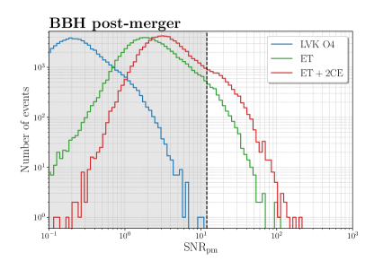
(a)

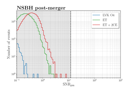
(b)

Figure 24: Histograms of the SNR in the post–merger phase of BBH binaries (left panel) and NSBH binaries (right panel), for 1 year of data. For BBHs the computation is performed using the IMRPhenomHM waveform, while for NSBH systems we adopted IMRPhenomNSBH.

Some properties of ‘golden events’ for BNS can be appreciated from Fig. 15 for ET, and from Fig. 16 for ET+2CE. Given that BNS are intrinsically less loud, now meaningful cuts are at lower values of the SNR. With our fiducial choice for the population, at ET there are $\order{800}$ events per year at with ${\rm SNR}\geq 30$, $\order{150}$ with ${\rm SNR}\geq 50$, and $\order{20}$ with ${\rm SNR}\geq 100$, of which, in our sample, the farthest is at $z\simeq 0.19$. It is important to notice that these results have been obtained setting ${\cal R}_{0,{\rm BNS}}=$105.5\text{\,}{\mathrm{Gpc}}^{-3}\text{\,}{\mathrm{yr}}^{-1}$$ and, as we repeatedly stressed, there is an uncertainty of one order of magnitude, in both directions, on this number. Similarly to the case of BBHs, for ET+2CE there is a further improvement by typically one order of magnitude, both for the number of sources with a given high value of the SNR and for those with a small value of $\Delta d_{L}/d_{L}$. For instance, the number of BNS/yr with ${\rm SNR}\geq 50$ is $\order{1200}$. As usual, the improvement is even more important on the localization, thanks to triangulation. While, for ET alone, there are just about $\order{10}$ BNS/yr localized to better than $50\text{\,}{\mathrm{deg}}^{2}$, with ET+2CE there are $\order{2400}$ BNS/yr localized to better than $10\text{\,}{\mathrm{deg}}^{2}$, including events up to $z\sim 1.5$, and $\order{100}$ events/yr localized to better than $1\text{\,}{\mathrm{deg}}^{2}$, including events up to $z\sim 0.44$. To put this result in the correct perspective, however, it is useful to recall, from the discussion in Sect. 5.2, that, for multi–messenger observations, localization regions of the order of hundreds of square degree, as can be obtained by ET alone, are already sufficient to trigger the search of a kilonova with large FOV telescopes, which are then needed to localize the source to the arcsec precision necessary to point instruments such as the ELT and perform spectroscopic studies. However, the remarkable improvement in localization between ET and ET+2CE will be very important in some cosmological applications, such as those making use of dark sirens by correlating them with galaxy catalogs.

Finally, Fig. 20 and 21 show the analogous results for NSBHs. ‘Golden events’ for NSBHs could be particularly interesting for cosmological applications, since these events, compared to BNSs, are louder because of the larger mass, while they could still have an electromagnetic counterpart, if the NS is tidally disrupted during the merger; furthermore, while the spin of NSs in binaries is expected to be negligible, the spin of the BH in a NSBH binary in general might not be small (see, however, Mandel & Fragos (2020); Broekgaarden & Berger (2021); Mandel & Smith (2021)) and, if it induces a precession of the orbital plane, it can lift the degeneracy between $d_{L}$ and $\cos\iota$, leading to an improved distance measurement (Vitale & Chen, 2018). The plots in Fig. 20 and 21 show a pattern intermediate between that for BBHs and that for BNSs. This is expected since, as discussed in Sect. 4.1, for the models that we have used, the typical BH mass in a NSBH binary is of order $8\text{\,}\mathrm{M_{\odot}}$, so these systems are heavier than BNSs, but lighter than typical BBHs and, in the bandwidth of 3G detectors, they are louder than typical BNS, but weaker than typical BBHs. Finally, we observe that NSBH binaries look less promising than BBHs for testing the post–merger and ringdown phase of the final BH. In the right panel of Fig. 24 we show the distribution of ${\rm SNR}_{\rm pm}$ for these systems, which shows that the signal–to–noise ratio in the post–merger phase never exceed 10, even for ET+2CE.

6 Conclusions

In this paper we have performed a comprehensive study of the capabilities of the Einstein Telescope, alone and in a network with two Cosmic Explorer detectors, and we have also provided forecasts for the forthcoming LVK–O4 run. The results have been obtained using a new parameter estimation code, GWFAST, conceived especially for application to third–generation GW detectors. Our results broadly confirm the overall picture obtained in other recent studies of 3G detectors (see in particular Maggiore et al. (2020); Borhanian & Sathyaprakash (2022); Harms et al. (2022); Ronchini et al. (2022), and references therein), on the extraordinary scientific potential of 3G detectors. We have applied our code to study populations of BBHs, BNSs and NSBH binaries. Compared to some of the other works devoted to forecast for 3G detectors, our results are more tuned toward ET, including detailed studies of what ET can do as a single detector; we used updated information on the astrophysical population from the LVK population studies based on the GWTC–3 catalog of detections; we used state–of–the–art waveforms for all these sources, and included the Earth’s motion in the detectors response, which is especially relevant for BNSs; we expanded the range of parameters on which inference is performed, including the spin of the BHs and the tidal deformability of NSs; we also presented the first systematic study of parameter estimation for NSBH binaries at 3G detectors.

From the technical point of view our code, which is presented in more detail in the companion paper Iacovelli et al. (2022), has been designed so to optimally exploit the parallel nature of the problem of computing a large number of Fisher matrices for independent events, by vectorizing the evaluation of the Fisher matrices even on a single CPU. This relies on the implementation of the waveforms in Python, resulting in a gain in computational speed, which motivates the name GWFAST. Furthermore, this allows the use of automatic differentiation with the library JAX for the accurate computation of derivatives. Together with this paper, we publicly release the code GWFAST , which is available at https://github.com/CosmoStatGW/gwfast. This paper is associated to version v1.0.1 which is archived on Zenodo (Iacovelli & Mancarella, 2022). We also release the library WF4Py , available at https://github.com/CosmoStatGW/WF4Py, which contains state–of–the–art gravitational–wave waveforms in pure Python. This paper is associated to version v1.0.0 which is archived on Zenodo (Iacovelli, 2022).

Appendix A Details of the adopted population distributions

Here we report the shape and parameters of the population distributions mentioned in the main text. All these are available in the public code MGCosmoPop (Mancarella et al., 2022), together with sampling routines, which we used to obtain the catalogs.

A.1 Redshift distribution

For the BBH merger distribution with redshift we adopt a model that follows the star formation rate. As a caveat, we mention that this is just a first approximation, and other effects could induce departures from the star formation rate. In particular, metallicity–dependent effects might significantly boost the merger rate at low metallicities, see Santoliquido et al. (2021a) (in particular their Fig. 2) and Chruślińska (2022). Given the current uncertainties, a simple model of the merger rate following the star formation rate can be considered a meaningful starting point that, however, will have to be updated as our understanding of the merger rate of compact objects sharpens.

The Madau–Dickinson profile (Madau & Dickinson, 2014) for the star formation rate density has the functional form (Madau & Fragos, 2017)

$$\psi(z|\alpha_{z},\beta_{z},z_{p})\propto\frac{(1+z)^{\alpha_{z}}}{1+\left(\frac{1+z}{1+z_{p}}\right)^{\alpha_{z}+\beta_{z}}}\,.$$ (A1)

Observationally, the merger rate evolution of BBHs is currently constrained only at small redshift; assuming a profile $\psi(z|\kappa)\propto(1+z)^{\kappa}$, the analysis of the first three LVK observing runs gives the median value $\kappa=2.7$. Here we use the Madau–Dickinson profile, with the low–redshift slope fixed to the value of $\alpha_{z}=2.7$. This is chosen to match the value of $\kappa$ since at low redshift the Madau–Dickinson profile reduces to $\sim(1+z)^{\alpha_{z}}$. For the other parameters, we fix them to $\beta_{z}=3$ and $z_{p}=2$, which, within current uncertainties, are typical values used in the literature (Madau & Dickinson, 2014).

For BNS systems, instead, we convolve the Madau–Dickinson profile with a time delay distribution $P(t_{d})\propto 1/t_{d}$, using a minimum time delay of $20\text{\,}\mathrm{Myr}$, as suggested in Regimbau et al. (2012). To get a faster software implementation, we further re–fit the curve obtained after the convolution to another Madau–Dickinson profile, with new parameters $\alpha_{z}$, $\beta_{z}$ and $z_{p}$ now determined from the fit; we obtain the values $\alpha_{z}=1.42$, $\beta_{z}=4.62$, $z_{p}=1.84$, and this is what we use to generate the population (the overall rescaling to the local rate is discarded, since we always simulate a fixed amount of sources). A population with the same parameters is also adopted for NSBH systems.

The distribution in redshift of the merger rate of compact binaries is finally

$$p_{z}(z)\propto\psi(z|\alpha_{z},\beta_{z},z_{p})\frac{1}{1+z}\dfrac{{\rm d}V_{c}}{{\rm d}z}(z)\,,$$ (A2)

where ${\rm d}V_{c}/{\rm d}z$ is the comoving volume element and the factor of $1+z$ relates the source times and the observer time. In a flat $\Lambda$CDM Universe, the redshift is related to the luminosity distance of the source by

$$d_{L}(z)=(1+z)\dfrac{c}{H_{0}}\int_{0}^{z}\dfrac{{\rm d}\tilde{z}}{\sqrt{\Omega_{m}(1+\tilde{z})^{3}+\Omega_{\Lambda}}}\,,$$ (A3)

(the contribution of radiation is negligible even at the redshifts explored by 3G detectors), and we use Planck18 parameters (Planck Collaboration et al., 2020), i.e. $H_{0}=$67.66\text{\,}\mathrm{km}\text{\,}{\mathrm{s}}^{-1}\text{\,}{\mathrm{Mpc}}^{-1}$$, $\Omega_{m}=0.3097$ and $\Omega_{\Lambda}=1-\Omega_{m}=0.6903$.

A.2 Mass distribution

The Power Law + Peak distribution (Abbott et al., 2021c) used for the BBH mass function has the functional form, for the mass of the primary component (always taken as the heaviest),

$$p(m_{1}|\lambda_{\rm peak},\alpha,m_{\rm min},\delta_{m},m_{\rm max},\mu_{m},\sigma_{m})=\left[(1-\lambda_{\rm peak})\mathcal{P}(m_{1}|-\alpha,m_{\rm max})+\lambda_{\rm peak}\mathcal{N}(m_{1}|\mu_{m},\sigma_{m})\right]S(m_{1}|m_{\rm min},\delta_{m})$$ (A4)

where $\mathcal{P}(m_{1}|-\alpha,m_{\rm max})$ is a normalized power–law distribution with spectral index $-\alpha$ and high–mass cut–off $m_{\rm max}$, $\mathcal{N}(m_{1}|\mu_{m},\sigma_{m})$ is a normalised Gaussian distribution with mean $\mu_{m}$ and standard deviation $\sigma_{m}$, while $S(m_{1}|m_{\rm min},\delta_{m})$ is a smoothing function of the form

$$S(m_{1}|m_{\rm min},\delta_{m})=\begin{dcases}0&(m<m_{\rm min})\\ [f(m-m_{\rm min},\delta_{m})+1]^{-1}&(m_{\rm min}\leq m<m_{\rm min}+\delta_{m})\\ 1&(m\geq m_{\rm min}+\delta_{m})\end{dcases}\,,$$ (A5)

with

$$f(m^{\prime},\delta_{m})={\rm exp}\left\{\dfrac{\delta_{m}}{m^{\prime}}+\dfrac{\delta_{m}}{m^{\prime}-\delta_{m}}\right\}.$$ (A6)

The conditional mass ratio distribution of this model is

$$p(q|\beta_{q},m_{1},m_{\rm min},\delta_{m})\propto q^{\beta_{q}}S(qm_{1}|m_{\rm min},\delta_{m}).$$ (A7)

The numerical values of the parameters we used for this distribution are $\lambda_{\rm peak}=0.039,\ \alpha=3.4,\ m_{\rm min}=5.1,\ \delta_{m}=4.8,\ m_{\rm max}=87,\ \mu_{m}=34,\ \sigma_{m}=3.6,\ \beta_{q}=1.1$.³⁵

A.3 Spin distribution

The Default distribution used to simulate the BBH spins [introduced in Abbott et al. (2019c)] assumes a Beta distribution for the spin magnitudes (taken to be independent)

$$p(\chi_{1,2}|\alpha_{\chi},\beta_{\chi})={\rm Beta}(\alpha_{\chi},\beta_{\chi})\,,$$ (A8)

while the orientations are drawn from

$$p({\bf z}|\zeta,\sigma_{t})=\zeta{\cal N}_{t}({\bf z}|0,\sigma_{t})+(1-\zeta){\rm I}({\bf z})\,,$$ (A9)

where $z_{i}={\rm cos}\theta_{i}$, $\theta_{i}$ is the tilt angle between the component spin and the binary’s orbital angular momentum, ${\cal N}_{t}({\bf z}|0,\sigma_{t})$ is a truncated Gaussian distribution centered at 0 and with standard deviation $\sigma_{t}$, while ${\rm I}({\bf z})$ denotes an isotropic distribution. Though this model could be used to sample all the 6 components of the spins of the two objects, we will always extract only the distribution of the spin component aligned with the orbital angular momentum, setting the others to zero. The numerical values of the parameters we used for this distribution are $\zeta=0.66,\ \sigma_{t}=1.5,\ \mu_{\chi}=0.28,\ \sigma_{\chi}=0.03$,³⁵ from which it follows $\alpha_{\chi}=1.6,\ \beta_{\chi}=4.12$.

Appendix B Comparison with other parameter estimation codes

With the recent boost in activities for Einstein Telescope and Cosmic Explorer, parameter estimation for 3G detectors has become a particularly important topic, both as a tool to develop the science case for these detectors, and to inform the choices for optimal detector’s design and detector network configuration, so several parameter estimation codes have been developed recently. In this appendix we compare our code and our results to those obtained with GWBENCH (Borhanian, 2021; Borhanian & Sathyaprakash, 2022), developed at Penn State, and with GWFISH, developed by the GSSI group (Harms et al., 2022) which, together with GWFAST, are among the most complete and advanced codes available, for parameter estimation at 3G detectors [see also Chan et al. (2018); Grimm & Harms (2020); Nitz & Dal Canton (2021); Li et al. (2022); Pieroni et al. (2022)].

We begin by observing that, in the context of the activities of the ET Observational Science Board (OSB), our group, the GSSI group and the Penn State group have analyzed a small sample of common injections, using all the same waveform model [the TaylorF2 waveform, developed in Buonanno et al. (2009a)], finding excellent agreement, at the level of one part in $10^{4}-10^{5}$ for the SNR, and one part in $10^{3}$ on the parameter estimation of individual signals. This is an important consistency check for these rather complex codes, that had been developed totally independently. Further activity on this is in progress.

We next compare the results presented in our paper with those presented in Borhanian & Sathyaprakash (2022), and with those in Ronchini et al. (2022) (that provides an extensive set of results for BNSs obtained with GWFISH). The comparison must take into account the fact that, currently, there are large uncertainties on several aspects, ranging from the detector configurations considered, the assumptions on the astrophysical models, as well as several differences in technical details, such as the waveform models used, the assumed threshold for the SNR, down to different implementations of the Fisher matrix inversion. To orient the reader, we therefore find useful first of all to give a summary of several different choices adopted in these works. We stress that all these different choices are fully legitimate, and reflect current uncertainties. It is therefore instructive to see how the results change when using different assumptions. We also stress that, while the results, in our paper as well as in Borhanian & Sathyaprakash (2022) and in Harms et al. (2022); Ronchini et al. (2022), are necessarily presented just for a selection of few different choices, the codes themselves can be adapted to a larger variety of choices. The main differences in the assumptions used in these works can be summarized as follows.

Detector networks. Our work is more focused on ET. To avoid a proliferation of plots, or of lines in each plot, we only presented the results for two 3G configurations: ET alone, and ET+2CE. Studying ET alone allows us to assess the strength of the ET Science Case, independently of decisions that will be taken by different funding agencies on CE. On the other hand, combining ET with two CE detectors allows us to examine the full strength of a 3G detector network. The two CE detectors are assumed to be one with $40\text{\,}\mathrm{km}$ arms, and one with $20\text{\,}\mathrm{km}$ arms, which is the reference CE configuration (Evans et al., 2021). We set both of them in the U.S. (the other options that is under consideration, with one of them in Australia, allows better triangulation but, otherwise, is not very different). In contrast, in Ronchini et al. (2022) are studied ET alone, ET+CE ($40\text{\,}\mathrm{km}$) and ET+2CE, with both CE detectors with $40\text{\,}\mathrm{km}$ arms, and one of them located in Australia; compared to the ET+2CE network that we have studied, the latter network therefore has a greater horizon to coalescing binaries, because of the 40+40 km arms, and better sky localization, because one of the CE detectors is set in Australia. The work in Borhanian & Sathyaprakash (2022) studies a larger set of combinations of 2G⁺ and 3G configurations, somewhat more tuned toward CE. ET alone is not considered, but is studied in a so–called ‘ECS’ network, consisting of ET and 2CE, both having $40\text{\,}\mathrm{km}$ arms, with a CE located in Australia.

Astrophysical populations. In Borhanian & Sathyaprakash (2022) are given predictions for BBHs and BNSs, and Ronchini et al. (2022) focus on BNSs, while we provide predictions for BBHs, BNSs and NSBHs. As we repeatedly stressed in the text, there are currently large uncertainties on the BBH, BNS and NSBH populations, and the fiducial choices made in different works can be sensibly different, resulting potentially in differences as large as one order of magnitude.

For BNSs, we assume a redshift distribution of the merger rate given by a rather standard Madau–Dickinson distribution with a delay of 20 Myr between formation and merger, as described in App. A; the same choice, with the same time delay, is made in Borhanian & Sathyaprakash (2022), while Ronchini et al. (2022) use a different model, based on a catalog generated according to the recent study in Santoliquido et al. (2021a). Furthermore, the overall normalizations are different. Our fiducial value for the local rate is ${\cal R}_{0,\rm BNS}=$105.5\text{\,}{\mathrm{Gpc}}^{-3}\text{\,}{\mathrm{yr}}^{-1}$$, which is the median value for ${\cal R}_{0,\rm BNS}$ inferred from the GWTC–3 catalog, using the same flat mass distribution that we are using (Abbott et al., 2021c). In contrast, Borhanian & Sathyaprakash (2022) use ${\cal R}_{0,\rm BNS}=$320\text{\,}{\mathrm{Gpc}}^{-3}\text{\,}{\mathrm{yr}}^{-1}$$, which is the median value inferred from the GWTC–2 catalog (actually, with a flat mass distribution, while Borhanian & Sathyaprakash (2022) use a truncated Gaussian distribution), and Ronchini et al. (2022) use ${\cal R}_{0,\rm BNS}=$365\text{\,}{\mathrm{Gpc}}^{-3}\text{\,}{\mathrm{yr}}^{-1}$$ (with the same flat mass distribution between 1 and $2.5\text{\,}\mathrm{M_{\odot}}$ that we also use). As a result of these differences, the rate of BNS mergers in our population model is $1\text{\times}{10}^{5}$ events/yr, in Borhanian & Sathyaprakash (2022) is $4.7\text{\times}{10}^{5}$ events/yr, and in Ronchini et al. (2022) is $9\text{\times}{10}^{5}$. These numbers therefore span one full order of magnitude, and are the main reason for the differences among our results for BNSs. Our estimates are the most conservative among these works, but we stress again that all these assumptions are consistent with current knowledge, and, in fact, none of them are on the extreme side. As we mentioned, values of ${\cal R}_{0,\rm BNS}$ in the range $(10-1700)\leavevmode\nobreak\ ${\mathrm{Gpc}}^{-3}\text{\,}{\mathrm{yr}}^{-1}$$ are still consistent with current observations, so one could consider even more conservative, or even more optimistic models.

For BBHs, both us and Borhanian & Sathyaprakash (2022) use a Madau–Dickinson distribution (with negligible delay between formation and merger for us, and a delay of 10 Myr for Borhanian & Sathyaprakash (2022)). For the local rate, current constraints are more stringent than for BNSs. Still, we use ${\cal R}_{0,{\rm BBH}}=$17\text{\,}{\mathrm{Gpc}}^{-3}\text{\,}{\mathrm{yr}}^{-1}$$, which is the median value from GWTC–3, while Borhanian & Sathyaprakash (2022) use ${\cal R}_{0,{\rm BBH}}=$24\text{\,}{\mathrm{Gpc}}^{-3}\text{\,}{\mathrm{yr}}^{-1}$$ from GWTC–2. As a result, our BBH merger rate is $7.5\text{\times}{10}^{4}$ events/yr, while in Borhanian & Sathyaprakash (2022) is $1.2\text{\times}{10}^{5}$ events/yr.

Waveforms and detection model. A number of other differences are related to the waveforms and the detection model assumed. For BNS, we use the IMRPhenomD_NRTidalv2 waveform, as in Borhanian & Sathyaprakash (2022), which includes inspiral, merger, ringdown, as well as tidal effects, while Ronchini et al. (2022) uses TaylorF2, a simpler inspiral–only waveform, and truncates it at a frequency of the order of $4f_{\rm ISCO}$, where $f_{\rm ISCO}$ is the frequency at the innermost stable orbit [however, GWFISH can use all waveforms models of the LALSimulation (LIGO Scientific Collaboration, 2018)]. We all include the effect of the Earth’s rotation on the localization of the BNSs. For BBHs both us and Borhanian & Sathyaprakash (2022) use IMRPhenomHM, which includes higher modes. There is, however, a difference on the number of parameters on which the inference is performed, both for BBHs and BNSs. In Borhanian & Sathyaprakash (2022) the inference is performed on the standard set of 9 parameters $\{{\cal M}_{c},\ \eta,\ d_{L},\ \theta,\ \phi,\ \iota,\ \psi,\ t_{c},\ \Phi_{c}\}$, while we add to this list also the two parallel spin components $\chi_{1,z}$ and $\chi_{2,z}$ and, for BNS and NSBH systems, we also perform the inference on the tidal deformability parameters, see Sect. 5.

Another difference concerns the threshold for the SNR. A lower threshold on the SNR increases the number of detections, but (beside raising the false–alarm rate in an actual run) at the level of our analysis it makes less reliable the parameter estimation made with the Fisher matrix. In this work, we present the bulk of our results with a detection threshold ${\rm SNR}\geq 12$, while Borhanian & Sathyaprakash (2022) use ${\rm SNR}\geq 10$; in Ronchini et al. (2022), which is concerned with multi–messenger observation of BNS, ${\rm SNR}\geq 8$ is used for the detection in survey mode (which can be more appropriate to multi–messenger observations, given the temporal coincidence with the electromagnetic signal), but it has been checked that in pointing mode, where the sky localization is used, most of the events have ${\rm SNR}\geq 12$.

Another significant point, especially for detector networks, is the assumption on the duty cycle. In this work, as in Ronchini et al. (2022), for 3G detectors we have assumed an uncorrelated duty cycle of $85\%$ for each arm, while in Borhanian & Sathyaprakash (2022) a duty cycle of $100\%$ is assumed. As we showed in Fig. 7, including a realistic duty cycle results in long tails of events with poor accuracy on $\Delta d_{L}/d_{L}$ and, to lesser extent, of $\Delta\Omega_{90\%}$, which are missed assuming a $100\%$ duty cycle. The same remark applies to the results presented for BBHs in Pieroni et al. (2022), which agree with ours once we also assume a $100\%$ duty cycle.

As an example of the role of these different assumptions, we perform a more detailed comparison with the results reported in Ronchini et al. (2022) for the angular resolution of BNS at ET alone, shown in their Tab. 6, and in the cumulative distribution functions of their Figs. A1 and A2. In particular, they find that, at ET alone, one would detect $370\,{\rm events/yr}$ with $\Delta\Omega_{90\%}<$100\text{\,}{\mathrm{deg}}^{2}$$, and 2 events/yr with $\Delta\Omega_{90\%}<$1\text{\,}{\mathrm{deg}}^{2}$$, while, from the results in Sect. 5.2, we find $51\,{\rm events/yr}$ with $\Delta\Omega_{90\%}<$100\text{\,}{\mathrm{deg}}^{2}$$, and $2\,{\rm events/yr}$ event below $10\text{\,}{\mathrm{deg}}^{2}$. As a test, to isolate the effect of the choice of population, we have performed further runs using ${\cal R}_{0,\rm BNS}=$365\text{\,}{\mathrm{Gpc}}^{-3}\text{\,}{\mathrm{yr}}^{-1}$$, ${\rm SNR}\geq 8$ and the TaylorF2 waveform, so that the only difference is now in the model for the redshift evolution of the population. Under these conditions, in our model the population consists of $3.5\text{\times}{10}^{5}$ BNS mergers per year, to be compared with $9.0\text{\times}{10}^{5}$ in Ronchini et al. (2022), which is higher by a factor $\simeq 2.6$. Out of these mergers, we find that ET alone would detect $8.6\text{\times}{10}^{4}$ events/yr, to be compared with $1.4\text{\times}{10}^{5}$ events/yr in Ronchini et al. (2022), which is now larger only by a factor $\simeq 1.7$. This is due to the fact that the excess in the population used in Ronchini et al. (2022), compared to ours, is especially significant at large $z$ where, however, BNSs are more difficult to detect. Then, selecting the events with $\Delta\Omega_{90\%}<$1\text{\,}{\mathrm{deg}}^{2}$$, $10\text{\,}{\mathrm{deg}}^{2}$ and $100\text{\,}{\mathrm{deg}}^{2}$ we find, respectively, $(1,\,16,\,298)$ events/yr, to be compared with $(2,\,10,\,370)$ in Ronchini et al. (2022). Given the remaining difference in the redshift distribution of the population, we can then conclude that the results are fully consistent, once we make the same assumptions on local rate, and we use the SNR threshold and the same waveform. This underlines that, within current uncertainties of the rate and on the population model, and different choices for technical aspects such as waveform, SNR, etc, the results for BNSs can still vary sensibly. A comparison with the results reported in Borhanian & Sathyaprakash (2022) for their ECS configuration with our results for ET+2CE also show that our results broadly consistent, once taken into account the different rates, SNR threshold and network configuration.

Technical differences. Among the various technical aspects of the code, one worth mentioning here is the difference in the treatment of ill–conditioned Fisher matrices. In the present work these are discarded, on the basis of a criterion on the inversion error discussed in Sect. 2.2 and App. C. A similar strategy is adopted in GWBENCH, where the criterion is rather based on the condition number, i.e. the ratio of the largest to the smallest eigenvalue. In contrast, in GWFISH, ill–conditioned Fisher matrices are conditioned and inverted (i.e., after passing to a diagonal basis, the lines and columns corresponding to the eigenvector with almost vanishing eigenvalue are deleted, and the remaining reduced–order matrix is inverted) (Harms et al., 2022). This leads to treating a larger number of events with the Fisher matrix technique; however, the vanishing, or nearly vanishing, of an eigenvalue means that the linear approximation on which the Fisher matrix technique is based becomes invalid, and one must worry about the effect of non–linear contributions; the basis in parameter space that diagonalizes the likelihood at quadratic order, in general, will no longer diagonalize it when cubic and higher–order terms are included; so the parameter that, at quadratic order, has vanishing eigenvalue and is discarded, beyond quadratic order could have non–trivial correlations with all other parameters, possibly leading to larger marginalized errors on them, compared to the answer obtained from the quadratic approximation, i.e. from the Fisher matrix. For this reason, we have chosen to discard events with ill–conditioned Fisher matrices. In App. C we show a comparison of different techniques. Note that, however, GWFAST offers different choices, including the conditioning of the singular values, and the final choice is left to the user (see Iacovelli et al. (2022) for a detailed description).

As we see from Tab. 3, for BBHs the number of events that we have discarded because the Fisher matrix was ill–conditioned is about $4\%$ of the total number of detected events at ET, and just $0.3\%$ for ET+2CE. Therefore, at the population level, the effect is quite marginal. For BNSs we see from Tab. 4 that the number of events discarded is slightly higher but still consistent, $4.5\%$ at ET and $1.3\%$ at ET+2CE. The effect of different treatments of the problem could then in principle be relevant. On the other hand, discarding ill–conditioned matrices is not a perfect solution either, since it can potentially introduce some bias; for instance, events with $\cos\iota$ close to one are preferentially discarded, since in this limit the derivative with respect to $\iota$ vanishes. Basically, we are facing here an intrinsic limitations of the Fisher matrix technique, and it is reassuring that codes employing different approaches reach consistent conclusions. At present, the uncertainty in the results is completely dominated by the astrophysical uncertainties.

Appendix C Comparison among different ways to quantify uncertainty from the Fisher matrix

Parameter	Prior range
$\mathcal{M}_{c},\ d_{L}$	$(0,\,+\infty)$
$\eta$	$(0,\,0.25]$
$\phi,\ \Phi_{c}$	$[0,\,2\pi]$
$\theta,\ \iota,\ \psi,$	$[0,\,\pi]$
$t_{c}$	$[0,\,1]$
$\chi_{i,z}$ $(i=\{1,2\})$	$[-1,\,1]$
$\Lambda_{i}$ $(i=\{1,2\})$	$[0,\,+\infty)$

Table 6: Summary of the prior ranges used when sampling from the posterior probability.

In this appendix we provide a comparison among different methods of extracting the forecasted uncertainty on the waveform parameters from the Fisher matrix, which motivates our choice for this paper as discussed in Sect. 2.2. As a test case we use the sample of BNSs, which is generally the most prone to showing large condition numbers. In particular, discarding matrices with condition number higher than the inverse machine precision ($10^{-15}$ in our case) would lead to having only a few events left, which does not allow a statistical study of the population unless the even more stringent and less realistic assumption of discarding some parameters (e.g. neglecting the presence of spins and tidal deformabilities) is made. The options that we consider are (see Iacovelli et al. (2022) for a detailed description of the methods and their implementation in GWFAST):

1. we invert the Fisher matrix by a Cholesky decomposition, compute the inversion error as defined in Eq. (12), and exclude events with inversion error less than a chosen threshold $\epsilon_{\rm max}$. In particular, we compare the choices $\epsilon_{\rm max}=${10}^{-3}$$ and $\epsilon_{\rm max}=$5\text{\times}{10}^{-2}$$;

2. we invert all Fisher matrices by using the singular–value decomposition (SVD), and exclude from the inversion the singular values below a threshold of $10^{-10}$, to ensure that the numerical error does not propagate to well–measured parameters (Harms et al., 2022). Note that the inversion error is not defined in this case since the singular values of the matrix are regularized before inversion;

3. We impose physically–motivated priors on top of the likelihood in Eq. (11), draw samples from the corresponding posterior, and quantify the resulting forecasted uncertainty from the samples. This procedure is detailed below and does not require any inversion of the Fisher matrix, hence it is not sensitive to numerical instabilities and encodes the correct boundaries for the waveform parameters. On the other hand, this technique is computationally too expensive to be used for all catalogs; we only resort to it in this case for a validation of the forecasts.

Let us describe the method used for the third option. The posterior probability for source parameters ${\bf\it\theta}$ given data $s$ is defined as $p({\bf\it\theta}\,|\,s)\propto\pi({{\bf\it\theta}})\,\mathcal{L}(s\,|\,{\bf\it\theta})$ where the likelihood $\mathcal{L}(s\,|\,{\bf\it\theta})$ is defined in Eq. (11) and $\pi({{\bf\it\theta}})$ is the chosen prior. We use flat priors with the boundaries summarized in Tab. 6 and also fix $\langle{\delta\theta}^{i}\rangle=0$, i.e. we assume that the posterior mean coincides with the true value, that we denote by ${\bf\it\mu}$. This is the same assumption made when quantifying the uncertainty directly from the Fisher matrix. Written in the form of Eq. (11), the evaluation of the likelihood does not require the explicit inversion of the Fisher Matrix, and one can extract samples from this distribution. For each event in the simulated catalogue of detections, we draw samples from the corresponding posterior by the following procedure:

1. for variables whose $1\sigma$ uncertainty as forecasted by the Fisher analysis is larger than the prior range, we add a Gaussian prior with standard deviation equal to the prior range; this has only the purpose of improving the efficiency and numerical stability, and such prior is undone during the sampling procedure;

2. We sample from the likelihood Eq. (11) as follows. First, we generate a vector ${\bf\it z}=(z_{1},\ ...,\ z_{D})$ of independent, standard normal variables (with $D$ being the dimensionality of the Fisher matrix). Then, we find the Cholesky decomposition ${\bf\it C}$ of the Fisher matrix ${\bf\it\Gamma}$, such that ${\bf\it C}{\bf\it C}^{T}={\bf\it\Gamma}$. Note that this decomposition might not be found if the Fisher matrix is ill–conditioned, hence the need of the Gaussian prior discussed in the previous step, which ensures regularization. Then, the desired samples are given by ${\bf\it\mu}+{\bf\it X}$ where ${\bf\it X}$ is the solution of the system ${\bf\it C}^{T}{\bf\it X}={\bf\it z}$, and ${\bf\it\mu}$ the vector of the true values;

3. We use rejection sampling to discard samples outside the prior range, as well as to undo the Gaussian prior previously imposed to regularize the Fisher matrix.

The uncertainty is finally quantified by computing the standard deviation of the samples. The only caveat concerns the use of Eq. (28) to determine the sky localization, since its derivation assumes a multivariate Gaussian distribution, while the use of priors can spoil this assumption. Hence we compute the $90\%$ sky localization by projecting the samples on the sphere with a HEALPix pixelization (Zonca et al., 2019), locating the pixels within the $90\%$ localization region, and computing the corresponding sky area. This procedure is exact, but can require a very extensive and expensive sampling for events whose localization is not well determined. A second caveat is that the number of pixels used must be adapted on an event–by–event basis. In order to reduce the computational cost, we only extract $2000$ samples/event, which can make this procedure underestimate the sky localization for poorly localized sources. However, this is enough for an accurate computation for well–localized events, in which case this provides an important numerical confirmation of the validity of Eq. (28). As an alternative check, we compute the sky localization by binning the samples in $(\theta,\phi)$, finding the bins within the $90\%$ localization region, and computing the corresponding area on the sphere. This procedure does not require a large number of samples, but it is sensitive to the number of bins used, which is a quantity that has to be fixed a priori, and whose mis–specification can lead to wrong estimates. In summary, there is no fast and $100\%$ accurate way to compute the localization region, but comparing the techniques listed above we will show that the different techniques agree very well for events with sufficiently small ($\lesssim 10^{3}\ \rm deg^{2}$) localization region.

Fig. 25 and Fig. 26 summarize our results. We show the cumulative distribution of the forecasted $1\sigma$ errors on the detector–frame chirp mass, symmetric mass ratio, luminosity distance, $90\%$ sky localization and spins along the $z$ axis, which are the most interesting for the discussion. Fig. 25 shows the results for ET alone, while Fig. 26 for ET and two CE. From these figures we can draw a number of interesting conclusions.

First, we see that for the left tails of the distributions, corresponding to well–resolved events, the result obtained with the SVD inversion and regularization (green curve) and the one obtained setting a threshold on the inversion error of $\epsilon_{\rm max}=$5\text{\times}{10}^{-2}$$ (orange curve) agree almost perfectly for all variables except the spin, in which case the regularization of the singular values leads to severely underestimating the error. We conclude that degeneracies among the spin parameters are those that mostly affect the condition number and lead to the presence of very small singular values, which are consequently regularized. Hence, the regularization procedure should not be adopted if one is interested in forecasting errors on spin parameters. Secondly we note that, adopting a threshold on the inversion error which is too stringent, such as $\epsilon_{\rm max}=${10}^{-3}$$ (blue curves), can lead to missing the tail of the best resolved events for some parameters, in particular the chirp mass. On the contrary, the choice $\epsilon_{\rm max}=$5\text{\times}{10}^{-2}$$ ensures that all the lower tails of the distributions match perfectly both the distribution obtained with SVD and the one obtained by sampling (red curves). This motivates the choice of this threshold in this paper.

Finally, we comment on the errors obtained with the sampling procedure (red curves). As expected, the left tail of the distributions, corresponding to very–well measured parameters, match the results obtained by the inversion of the Fisher matrix. In general, the use of priors affects differently different parameters and different configurations. For the mass parameters, we note a general improvement, which can be explained by the fact that most of the detected events lie very close to the threshold value $\eta=0.25$ for the symmetric mass ratio. This leads the finite prior range $\eta\leq 0.25$ to play a significant role in reducing the forecasted uncertainty; in turn, it also affects the constraint on the chirp mass, due to the correlation of this parameter with $\eta$. Similarly, the relative error on the luminosity distance is reduced at ET alone by the use of a prior because this reduces the allowed range for the inclination angle $\iota$, whose degeneracy with $d_{L}$ contributes significantly to the error on the latter. For ET in combination with two CE, this effects is mitigated because $\iota$ is generally better constrained without the need of a prior. As for the spins, these are generally poorly constrained and subject to strong degeneracies among the two components; this explains the improvement given by the prior. We conclude with the sky localization. The red curve corresponds to the results obtained by the binning procedure described above, while we additionally show in violet the results obtained by the HEALPix projection. As anticipated, both methods match well the forecast obtained by the Fisher matrix alone for $\Delta\Omega_{90\%}\lesssim 10^{3}\ \rm deg^{2}$, providing a confirmation of Eq. (28). The use of priors has a larger effect on the forecasts for ET alone, because for this configuration a precise localization is more difficult. In this sense, the Fisher forecast provides a conservative estimation of the localization capabilities. The method based on HEALPix (violet lines) shows some disagreement for localization regions larger than $\sim 10^{3}\ \rm deg^{2}$, due to the limited number of samples available, which do not sufficiently cover all the pixels. Drawing more samples would lead to better convergence also of the upper tail. This results confirm that the use of of Eq. (28) is reliable for all events with sufficiently small localization regions.

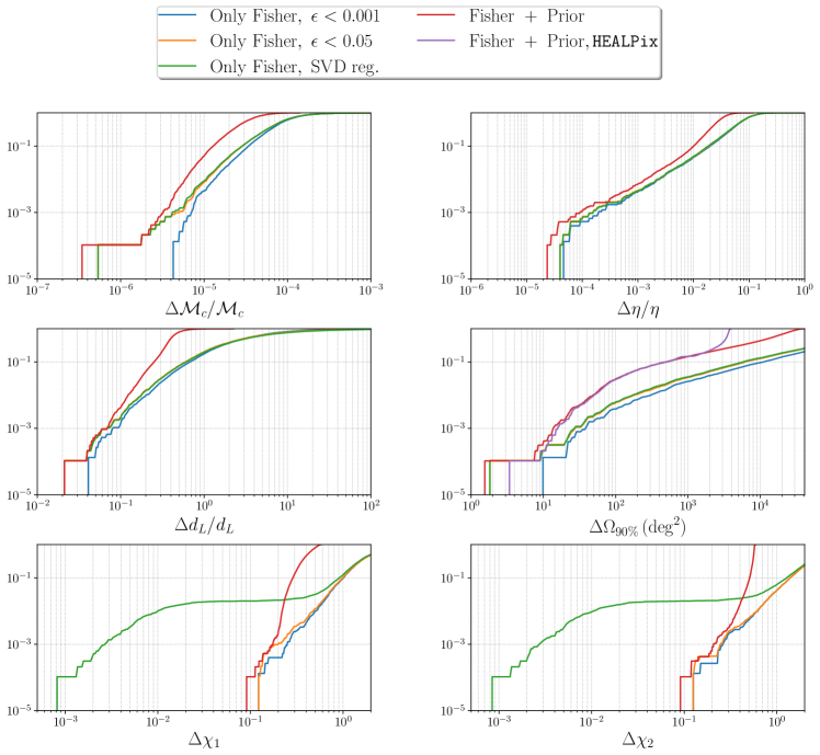
Figure 25: Comparison of cumulative distributions of the errors on the detector–frame chirp mass, symmetric mass ratio, luminosity distance, $90\%$ sky localization and spin components along the $z$ axis, for BNS observed at ET, with different choices to quantify the uncertainty. The default choice for this paper, $\epsilon<0.05$, corresponds to the orange curve.

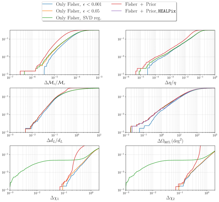
Figure 26: As in Fig. 25, for a network of ET and two CE.

Appendix D Comparison with realistic neutron star equations of state

The equation of state (EoS) of dense matter above the nuclear density is still unknown, thus we cannot yet reliably relate the mass of a neutron star to its adimensional tidal deformability. In the main text we made the agnostic choice of sampling the tidal deformabilities of the simulated BNS systems from a uniform distribution with broad limits, while here we explore the impact of assuming a common equation of state for all BNS systems. In particular, we consider the so–called APR4 (Akmal et al., 1998) and ALF2 (Alford et al., 2005) EoS, as representative of soft and hard EoS, respectively. The former thus predicts more compact stars with respect to the latter, leading to smaller values of the adimensional tidal deformability parameter for the same mass, which seems to be favoured by the observation of the BNS event GW170817 (Abbott et al., 2017a). The results, for the ET + 2CE network only, are shown in Fig. 27, where we compare sources having the same parameters apart from the tidal deformability, which in the case of the green curve is sampled uniformly in the interval $[0,\,2000]$, while for the others is computed from the mass of the two components assuming one of the chosen EoS. Notice that the uniform distribution used in the main text for the BNS masses, ranging up to $2.5\text{\,}\mathrm{M_{\odot}}$, is not suitable for performing this test, given that it exceeds the maximum masses of the chosen EoS. To perform this analysis we thus adopted two independent Gaussian distribution for the masses of the components, ${\cal N}(1.33,0.09)$ in units of $\mathrm{M_{\odot}}$. From the plot it is apparent that different choices for the tidal deformability distribution have negligible impact on the distributions of the parameter errors apart from the tidal deformability itself. In particular, we find the stiff EoS to produce systems whose relative error on the adimensional tidal deformability parameter is smaller, as compared to the soft. This is in line with the fact that a stiffer EoS predicts higher values for the adimensional tidal deformability parameter, so the effect on the waveform is larger, which makes the estimation easier. This also provides a consistency check of our code. We thus conclude that our results for BNS systems are robust with respect to different choices for the adimensional tidal deformability distribution.

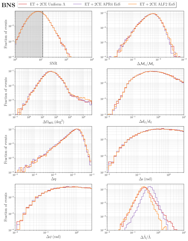
Figure 27: Histograms of the parameter errors for BNSs with the ET+2CE network configuration, using the waveform model IMRPhenomD_NRTidalv2, and sampling the tidal deformability uniformly in the interval $[0,\,2000]$ (red line), or assuming for all BNSs a common equation of state, chosen to be APR4 (violet) or ALF2 (orange).

Appendix E Comparison among different waveform models

We report here the comparison of the results for the SNR and parameter estimation errors for the three classes of sources, with waveform models different from the ones adopted in the main text. Again comparison is only made using the ET + 2CE detector network.

For BNS and NSBH systems, we compare the results obtained using the full inspiral–merger–ringdown models IMRPhenomD_NRTidalv2 and IMRPhenomNSBH, respectively, to the inspiral–only restricted PN model TaylorF2 with terms up to 3.5 order (Buonanno et al., 2009b; Ajith, 2011; Mishra et al., 2016), also including in it tidal effects (which enter at order 5 and 6 in the PN expansion) (Wade et al., 2014), and a cut at twice the Innermost Stable Circular Orbit frequency, $f_{\rm ISCO}$. As it is apparent from Fig. 28 and 29, the change in the distribution of SNRs and extrinsic parameters errors, i.e. the sky location, luminosity distance, inclination angle and polarisation angle, is slight, as expected, since these parameters are not linked to the waveform model itself in absence of higher modes, which are not expected to give strong contributions for these classes of sources. The situation is different for intrinsic parameters, i.e. the chirp mass, symmetric mass ratio, spins and tidal deformability, whose impact on the GW signal is obviously better captured by the full inspiral–merger–ringdown models, resulting in significant improvements in the estimation.

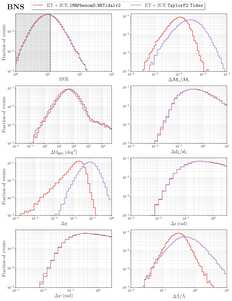
Figure 28: Histograms of the parameter errors for BNSs with the ET+2CE network configuration, using the full inspiral–merger–ringdown waveform model IMRPhenomD_NRTidalv2 and the 3.5 restricted PN model TaylorF2 with tidal effects.

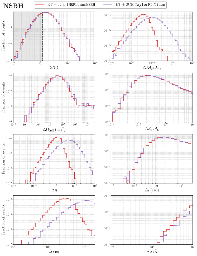
Figure 29: Histograms of the parameter errors for NSBH with the ET+2CE network configuration, using the full inspiral–merger–ringdown waveform model IMRPhenomNSBH and the 3.5 restricted PN model TaylorF2 with tidal effects.

References

- Abbott et al. (2017a) Abbott, B., et al. 2017a, Phys. Rev. Lett., 119, 161101, doi: 10.1103/PhysRevLett.119.161101
- Abbott et al. (2019a) —. 2019a, Phys. Rev. X, 9, 011001, doi: 10.1103/PhysRevX.9.011001
- Abbott et al. (2019b) —. 2019b, Phys. Rev. X, 9, 031040, doi: 10.1103/PhysRevX.9.031040
- Abbott et al. (2016) Abbott, B. P., et al. 2016, Phys. Rev. Lett., 116, 061102, doi: 10.1103/PhysRevLett.116.061102
- Abbott et al. (2017b) —. 2017b, Astrophys. J. Lett., 848, L13, doi: 10.3847/2041-8213/aa920c
- Abbott et al. (2019c) —. 2019c, Astrophys. J. Lett., 882, L24, doi: 10.3847/2041-8213/ab3800
- Abbott et al. (2020a) —. 2020a, The Astrophysical Journal Letters, 892, L3, doi: 10.3847/2041-8213/ab75f5
- Abbott et al. (2020b) —. 2020b, Living Rev. Rel., 23, 3, doi: 10.1007/s41114-020-00026-9
- Abbott et al. (2020c) Abbott, R., et al. 2020c, Phys. Rev. Lett., 125, 101102, doi: 10.1103/PhysRevLett.125.101102
- Abbott et al. (2020d) —. 2020d, Astrophys. J. Lett., 900, L13, doi: 10.3847/2041-8213/aba493
- Abbott et al. (2021a) —. 2021a, Phys. Rev. X, 11, 021053, doi: 10.1103/PhysRevX.11.021053
- Abbott et al. (2021b) —. 2021b. https://arxiv.org/abs/2111.03606
- Abbott et al. (2021c) —. 2021c, The population of merging compact binaries inferred using gravitational waves through GWTC-3. https://arxiv.org/abs/2111.03634
- Abbott et al. (2021d) —. 2021d. https://arxiv.org/abs/2112.06861
- Abbott et al. (2021e) —. 2021e. https://arxiv.org/abs/2111.03604
- Abbott et al. (2021f) —. 2021f, Astrophys. J. Lett., 913, L7, doi: 10.3847/2041-8213/abe949
- Abbott et al. (2021g) —. 2021g, The Astrophysical Journal Letters, 915, L5, doi: 10.3847/2041-8213/ac082e
- Ajith (2011) Ajith, P. 2011, Phys. Rev. D, 84, 084037, doi: 10.1103/PhysRevD.84.084037
- Ajith et al. (2006) Ajith, P., Hewitson, M., & Heng, I. S. 2006, Class. Quant. Grav., 23, S741, doi: 10.1088/0264-9381/23/19/S13
- Akmal et al. (1998) Akmal, A., Pandharipande, V. R., & Ravenhall, D. G. 1998, Phys. Rev. C, 58, 1804, doi: 10.1103/PhysRevC.58.1804
- Alford et al. (2005) Alford, M., Braby, M., Paris, M., & Reddy, S. 2005, The Astrophysical Journal, 629, 969, doi: 10.1086/430902
- Antonelli et al. (2021) Antonelli, A., Burke, O., & Gair, J. R. 2021, Mon. Not. Roy. Astron. Soc., 507, 5069, doi: 10.1093/mnras/stab2358
- Barack & Cutler (2004) Barack, L., & Cutler, C. 2004, Phys. Rev. D, 69, 082005, doi: 10.1103/PhysRevD.69.082005
- Bavera et al. (2022) Bavera, S. S., Fishbach, M., Zevin, M., Zapartas, E., & Fragos, T. 2022. https://arxiv.org/abs/2204.02619
- Belczynski et al. (2022) Belczynski, K., Doctor, Z., Zevin, M., et al. 2022. https://arxiv.org/abs/2204.11730
- Belgacem et al. (2019a) Belgacem, E., Dirian, Y., Foffa, S., et al. 2019a, JCAP, 1908, 015, doi: 10.1088/1475-7516/2019/08/015
- Belgacem et al. (2018a) Belgacem, E., Dirian, Y., Foffa, S., & Maggiore, M. 2018a, Phys. Rev. D, 97, 104066, doi: 10.1103/PhysRevD.97.104066
- Belgacem et al. (2018b) —. 2018b, Phys. Rev. D, 98, 023510, doi: 10.1103/PhysRevD.98.023510
- Belgacem et al. (2019b) Belgacem, E., et al. 2019b, JCAP, 1907, 024, doi: 10.1088/1475-7516/2019/07/024
- Berti et al. (2005) Berti, E., Buonanno, A., & Will, C. M. 2005, Phys. Rev. D, 71, 084025, doi: 10.1103/PhysRevD.71.084025
- Berti et al. (2016) Berti, E., Sesana, A., Barausse, E., Cardoso, V., & Belczynski, K. 2016, Phys. Rev. Lett., 117, 101102, doi: 10.1103/PhysRevLett.117.101102
- Biscoveanu et al. (2022) Biscoveanu, S., Callister, T. A., Haster, C.-J., et al. 2022, Astrophys. J. Lett., 932, L19, doi: 10.3847/2041-8213/ac71a8
- Borhanian (2021) Borhanian, S. 2021, Class. Quant. Grav., 38, 175014, doi: 10.1088/1361-6382/ac1618
- Borhanian et al. (2020) Borhanian, S., Dhani, A., Gupta, A., Arun, K., & Sathyaprakash, B. 2020, Astrophys. J. Lett., 905, L28, doi: 10.3847/2041-8213/abcaf5
- Borhanian & Sathyaprakash (2022) Borhanian, S., & Sathyaprakash, B. S. 2022, Listening to the Universe with Next Generation Ground-Based Gravitational-Wave Detectors. https://arxiv.org/abs/2202.11048
- Bradbury et al. (2018) Bradbury, J., Frostig, R., Hawkins, P., et al. 2018, JAX: composable transformations of Python+NumPy programs, 0.2.5. http://github.com/google/jax
- Broekgaarden & Berger (2021) Broekgaarden, F. S., & Berger, E. 2021, Astrophys. J. Lett., 920, L13, doi: 10.3847/2041-8213/ac2832
- Broekgaarden et al. (2021) Broekgaarden, F. S., Berger, E., Neijssel, C. J., et al. 2021, Mon. Not. Roy. Astron. Soc., 508, 5028, doi: 10.1093/mnras/stab2716
- Buonanno et al. (2009a) Buonanno, A., Iyer, B., Ochsner, E., Pan, Y., & Sathyaprakash, B. S. 2009a, Phys. Rev. D, 80, 084043, doi: 10.1103/PhysRevD.80.084043
- Buonanno et al. (2009b) Buonanno, A., Iyer, B. R., Ochsner, E., Pan, Y., & Sathyaprakash, B. S. 2009b, Phys. Rev. D, 80, 084043, doi: 10.1103/PhysRevD.80.084043
- Cardoso et al. (2016) Cardoso, V., Hopper, S., Macedo, C. F. B., Palenzuela, C., & Pani, P. 2016, Phys. Rev. D, 94, 084031, doi: 10.1103/PhysRevD.94.084031
- Chan et al. (2018) Chan, M. L., Messenger, C., Heng, I. S., & Hendry, M. 2018, Phys. Rev. D, 97, 123014, doi: 10.1103/PhysRevD.97.123014
- Chase et al. (2022) Chase, E. A., O’Connor, B., Fryer, C. L., et al. 2022, Astrophys. J., 927, 163, doi: 10.3847/1538-4357/ac3d25
- Chassande-Mottin et al. (2019) Chassande-Mottin, E., Leyde, K., Mastrogiovanni, S., & Steer, D. A. 2019, Phys. Rev. D, 100, 083514, doi: 10.1103/PhysRevD.100.083514
- Chatterji et al. (2006) Chatterji, S., Lazzarini, A., Stein, L., et al. 2006, Phys. Rev. D, 74, 082005, doi: 10.1103/PhysRevD.74.082005
- Chruślińska (2022) Chruślińska, M. 2022. https://arxiv.org/abs/2206.10622
- Cornish & Larson (2003) Cornish, N. J., & Larson, S. L. 2003, Phys. Rev. D, 67, 103001, doi: 10.1103/PhysRevD.67.103001
- Cowperthwaite et al. (2019) Cowperthwaite, P. S., Villar, V. A., Scolnic, D. M., & Berger, E. 2019, Astrophys. J., 874, 88, doi: 10.3847/1538-4357/ab07b6
- Cutler (1998) Cutler, C. 1998, Phys. Rev. D, 57, 7089, doi: 10.1103/PhysRevD.57.7089
- Cutler & Flanagan (1994) Cutler, C., & Flanagan, E. E. 1994, Phys. Rev. D, 49, 2658, doi: 10.1103/PhysRevD.49.2658
- De Luca et al. (2020) De Luca, V., Franciolini, G., Pani, P., & Riotto, A. 2020, JCAP, 06, 044, doi: 10.1088/1475-7516/2020/06/044
- De Luca et al. (2021a) —. 2021a, JCAP, 05, 003, doi: 10.1088/1475-7516/2021/05/003
- De Luca et al. (2021b) —. 2021b, JCAP, 11, 039, doi: 10.1088/1475-7516/2021/11/039
- Dietrich et al. (2019) Dietrich, T., Samajdar, A., Khan, S., et al. 2019, Phys. Rev. D, 100, 044003, doi: 10.1103/PhysRevD.100.044003
- Dominik et al. (2013) Dominik, M., Belczynski, K., Fryer, C., et al. 2013, Astrophys. J., 779, 72, doi: 10.1088/0004-637X/779/1/72
- Evans et al. (2021) Evans, M., et al. 2021. https://arxiv.org/abs/2109.09882
- Ezquiaga (2021) Ezquiaga, J. M. 2021, Phys. Lett. B, 822, 136665, doi: 10.1016/j.physletb.2021.136665
- Ezquiaga & Holz (2022) Ezquiaga, J. M., & Holz, D. E. 2022. https://arxiv.org/abs/2202.08240
- Farr et al. (2019) Farr, W. M., Fishbach, M., Ye, J., & Holz, D. 2019, Astrophys. J. Lett., 883, L42, doi: 10.3847/2041-8213/ab4284
- Farrow et al. (2019) Farrow, N., Zhu, X.-J., & Thrane, E. 2019, Astrophys. J., 876, 18, doi: 10.3847/1538-4357/ab12e3
- Finke et al. (2021) Finke, A., Foffa, S., Iacovelli, F., Maggiore, M., & Mancarella, M. 2021, JCAP, 08, 026, doi: 10.1088/1475-7516/2021/08/026
- Finke et al. (2022) —. 2022, Phys. Dark Univ., 36, 100994, doi: 10.1016/j.dark.2022.100994
- Finn (1992) Finn, L. S. 1992, Phys. Rev. D, 46, 5236, doi: 10.1103/PhysRevD.46.5236
- Fishbach et al. (2021) Fishbach, M., Doctor, Z., Callister, T., et al. 2021. https://arxiv.org/abs/2101.07699
- Franciolini (2021) Franciolini, G. 2021, PhD thesis, Geneva U., Dept. Theor. Phys., doi: 10.13097/archive-ouverte/unige:156136
- Freise et al. (2009) Freise, A., Chelkowski, S., Hild, S., et al. 2009, Classical and Quantum Gravity, 26, 085012, doi: 10.1088/0264-9381/26/8/085012
- García-Quirós et al. (2020) García-Quirós, C., Colleoni, M., Husa, S., et al. 2020, Phys. Rev. D, 102, 064002, doi: 10.1103/PhysRevD.102.064002
- Giacobbo & Mapelli (2018) Giacobbo, N., & Mapelli, M. 2018, Monthly Notices of the Royal Astronomical Society, 480, 2011, doi: 10.1093/mnras/sty1999
- Goldberg et al. (1967) Goldberg, J. N., Macfarlane, A. J., Newman, E. T., Rohrlich, F., & Sudarshan, E. C. G. 1967, Journal of Mathematical Physics, 8, 2155, doi: 10.1063/1.1705135
- Goncharov et al. (2022) Goncharov, B., Nitz, A. H., & Harms, J. 2022, Utilizing the null stream of Einstein Telescope, arXiv. https://arxiv.org/abs/2204.08533
- Graham et al. (2020) Graham, M., et al. 2020, Phys. Rev. Lett., 124, 251102, doi: 10.1103/PhysRevLett.124.251102
- Grimm & Harms (2020) Grimm, S., & Harms, J. 2020, Phys. Rev. D, 102, 022007, doi: 10.1103/PhysRevD.102.022007
- Gupta et al. (2022) Gupta, P. K., Puecher, A., Pang, P. T. H., et al. 2022. https://arxiv.org/abs/2205.01182
- Gürsel & Tinto (1989) Gürsel, Y., & Tinto, M. 1989, Phys. Rev. D, 40, 3884, doi: 10.1103/PhysRevD.40.3884
- Hall & Evans (2019) Hall, E. D., & Evans, M. 2019, Class. Quant. Grav., 36, 225002, doi: 10.1088/1361-6382/ab41d6
- Harms et al. (2022) Harms, J., Dupletsa, U., Banerjee, B., et al. 2022. https://arxiv.org/abs/2205.02499
- Harry & Fairhurst (2011) Harry, I. W., & Fairhurst, S. 2011, Phys. Rev. D, 83, 084002, doi: 10.1103/PhysRevD.83.084002
- Hernandez Vivanco et al. (2019) Hernandez Vivanco, F., Smith, R., Thrane, E., et al. 2019, Phys. Rev. D, 100, 103009, doi: 10.1103/PhysRevD.100.103009
- Hild et al. (2011) Hild, S., et al. 2011, Class. Quant. Grav., 28, 094013, doi: 10.1088/0264-9381/28/9/094013
- Himemoto et al. (2021) Himemoto, Y., Nishizawa, A., & Taruya, A. 2021, Phys. Rev. D, 104, 044010, doi: 10.1103/PhysRevD.104.044010
- Hinderer et al. (2010) Hinderer, T., Lackey, B. D., Lang, R. N., & Read, J. S. 2010, Phys. Rev. D, 81, 123016, doi: 10.1103/PhysRevD.81.123016
- Husa et al. (2016) Husa, S., Khan, S., Hannam, M., et al. 2016, Phys. Rev. D, 93, 044006, doi: 10.1103/PhysRevD.93.044006
- Iacovelli (2022) Iacovelli, F. 2022, WF4Py: Gravitational waves waveform models in pure Python language, v1.0.0, Zenodo, doi: 10.5281/zenodo.7060240
- Iacovelli & Mancarella (2022) Iacovelli, F., & Mancarella, M. 2022, gwfast: a Fisher information matrix Python package for GW detector networks, v1.0.1, Zenodo, doi: 10.5281/zenodo.7060236
- Iacovelli et al. (2022) Iacovelli, F., Mancarella, M., Foffa, S., & Maggiore, M. 2022, Astrophys. J. Suppl., To appear. https://arxiv.org/abs/2207.06910
- Ivezić et al. (2019) Ivezić, v., et al. 2019, Astrophys. J., 873, 111, doi: 10.3847/1538-4357/ab042c
- Jaranowski et al. (1998) Jaranowski, P., Królak, A., & Schutz, B. F. 1998, Phys. Rev. D, 58, 063001, doi: 10.1103/PhysRevD.58.063001
- Jin-Ping et al. (2021) Jin-Ping, Z., Shichao, W., Yuan-Pei, Y., et al. 2021, Astrophys. J., 917, 24, doi: 10.3847/1538-4357/abfe5e
- Kalaghatgi et al. (2020) Kalaghatgi, C., Hannam, M., & Raymond, V. 2020, Phys. Rev. D, 101, 103004, doi: 10.1103/PhysRevD.101.103004
- Kalogera et al. (2021) Kalogera, V., et al. 2021. https://arxiv.org/abs/2111.06990
- Karathanasis et al. (2022) Karathanasis, C., Mukherjee, S., & Mastrogiovanni, S. 2022. https://arxiv.org/abs/2204.13495
- Keelin (2016) Keelin, T. W. 2016, Decision Analysis, 13, 243, doi: 10.1287/deca.2016.0338
- Khan et al. (2016a) Khan, S., Husa, S., Hannam, M., et al. 2016a, Phys. Rev. D, 93, 044007, doi: 10.1103/PhysRevD.93.044007
- Khan et al. (2016b) —. 2016b, Phys. Rev. D, 93, 044007, doi: 10.1103/PhysRevD.93.044007
- Kinugawa et al. (2014) Kinugawa, T., Inayoshi, K., Hotokezaka, K., Nakauchi, D., & Nakamura, T. 2014, Mon. Not. Roy. Astron. Soc., 442, 2963, doi: 10.1093/mnras/stu1022
- Lattimer & Schramm (1976) Lattimer, J. M., & Schramm, D. N. 1976, ApJ, 210, 549, doi: 10.1086/154860
- Leyde et al. (2022) Leyde, K., Mastrogiovanni, S., Steer, D. A., Chassande-Mottin, E., & Karathanasis, C. 2022. https://arxiv.org/abs/2202.00025
- Li et al. (2022) Li, Y., Heng, I. S., Chan, M. L., Messenger, C., & Fan, X. 2022, Phys. Rev. D, 105, 043010, doi: 10.1103/PhysRevD.105.043010
- LIGO Scientific Collaboration (2018) LIGO Scientific Collaboration. 2018, LIGO Algorithm Library - LALSuite, free software (GPL), doi: 10.7935/GT1W-FZ16
- London et al. (2018) London, L., Khan, S., Fauchon-Jones, E., et al. 2018, Phys. Rev. Lett., 120, 161102, doi: 10.1103/PhysRevLett.120.161102
- Madau & Dickinson (2014) Madau, P., & Dickinson, M. 2014, Ann. Rev. Astron. Astrophys., 52, 415, doi: 10.1146/annurev-astro-081811-125615
- Madau & Fragos (2017) Madau, P., & Fragos, T. 2017, Astrophys. J., 840, 39, doi: 10.3847/1538-4357/aa6af9
- Maggiore (2007) Maggiore, M. 2007, Gravitational Waves. Vol. 1: Theory and Experiments, Oxford Master Series in Physics (Oxford University Press)
- Maggiore et al. (2020) Maggiore, M., et al. 2020, JCAP, 2003, 050, doi: 10.1088/1475-7516/2020/03/050
- Mancarella et al. (2022) Mancarella, M., Genoud-Prachex, E., & Maggiore, M. 2022, Phys. Rev. D, 105, 064030, doi: 10.1103/PhysRevD.105.064030
- Mandel & Broekgaarden (2022) Mandel, I., & Broekgaarden, F. S. 2022, Living Rev. Rel., 25, 1, doi: 10.1007/s41114-021-00034-3
- Mandel & Fragos (2020) Mandel, I., & Fragos, T. 2020, Astrophys. J. Lett., 895, L28, doi: 10.3847/2041-8213/ab8e41
- Mandel & Smith (2021) Mandel, I., & Smith, R. J. E. 2021, Astrophys. J. Lett., 922, L14, doi: 10.3847/2041-8213/ac35dd
- Margossian (2018) Margossian, C. C. 2018, CoRR, abs/1811.05031
- Mastrogiovanni et al. (2021a) Mastrogiovanni, S., Haegel, L., Karathanasis, C., Magana-Hernandez, I., & Steer, D. 2021a, JCAP, 02, 043, doi: 10.1088/1475-7516/2021/02/043
- Mastrogiovanni et al. (2021b) Mastrogiovanni, S., Leyde, K., Karathanasis, C., et al. 2021b, Phys. Rev. D, 104, 062009, doi: 10.1103/PhysRevD.104.062009
- McKernan et al. (2019) McKernan, B., Ford, K. E. S., Bartos, I., et al. 2019, Astrophys. J. Lett., 884, L50, doi: 10.3847/2041-8213/ab4886
- Meacher et al. (2016) Meacher, D., Cannon, K., Hanna, C., Regimbau, T., & Sathyaprakash, B. S. 2016, Phys. Rev. D, 93, 024018, doi: 10.1103/PhysRevD.93.024018
- Mink & King (2017) Mink, S. E. d., & King, A. 2017, Astrophys. J. Lett., 839, L7, doi: 10.3847/2041-8213/aa67f3
- Mishra et al. (2016) Mishra, C. K., Kela, A., Arun, K. G., & Faye, G. 2016, Phys. Rev. D, 93, 084054, doi: 10.1103/PhysRevD.93.084054
- Ng et al. (2022) Ng, K. K. Y., Franciolini, G., Berti, E., et al. 2022. https://arxiv.org/abs/2204.11864
- Ng et al. (2021a) Ng, K. K. Y., Vitale, S., Farr, W. M., & Rodriguez, C. L. 2021a, Astrophys. J. Lett., 913, L5, doi: 10.3847/2041-8213/abf8be
- Ng et al. (2021b) Ng, K. K. Y., Chen, S., Goncharov, B., et al. 2021b. https://arxiv.org/abs/2108.07276
- Nissanke et al. (2010) Nissanke, S., Holz, D. E., Hughes, S., Dalal, N., & Sievers, J. L. 2010, Astrophys. J., 725, 496, doi: 10.1088/0004-637X/725/1/496
- Nitz & Dal Canton (2021) Nitz, A. H., & Dal Canton, T. 2021, Astrophys. J. Lett., 917, L27, doi: 10.3847/2041-8213/ac1a75
- Palmese et al. (2021a) Palmese, A., Bom, C. R., Mucesh, S., & Hartley, W. G. 2021a. https://arxiv.org/abs/2111.06445
- Palmese et al. (2021b) Palmese, A., Fishbach, M., Burke, C. J., Annis, J. T., & Liu, X. 2021b, Astrophys. J. Lett., 914, L34, doi: 10.3847/2041-8213/ac0883
- Pannarale et al. (2015) Pannarale, F., Berti, E., Kyutoku, K., Lackey, B. D., & Shibata, M. 2015, Phys. Rev. D, 92, 084050, doi: 10.1103/PhysRevD.92.084050
- Perna et al. (2016) Perna, R., Lazzati, D., & Giacomazzo, B. 2016, Astrophys. J. Lett., 821, L18, doi: 10.3847/2041-8205/821/1/L18
- Pieroni et al. (2022) Pieroni, M., Ricciardone, A., & Barausse, E. 2022. https://arxiv.org/abs/2203.12586
- Pizzati et al. (2022) Pizzati, E., Sachdev, S., Gupta, A., & Sathyaprakash, B. 2022, Phys. Rev. D, 105, 104016, doi: 10.1103/PhysRevD.105.104016
- Planck Collaboration et al. (2020) Planck Collaboration, Aghanim, N., et al. 2020, A&A, 641, A6, doi: 10.1051/0004-6361/201833910
- Price-Whelan et al. (2018) Price-Whelan, A. M., Sipőcz, B. M., Günther, H. M., et al. 2018, The Astronomical Journal, 156, 123
- Prince et al. (2002) Prince, T. A., Tinto, M., Larson, S. L., & Armstrong, J. W. 2002, Phys. Rev. D, 66, 122002, doi: 10.1103/PhysRevD.66.122002
- Punturo et al. (2010) Punturo, M., et al. 2010, Class. Quant. Grav., 27, 194002, doi: 10.1088/0264-9381/27/19/194002
- Qin et al. (2018) Qin, Y., Fragos, T., Meynet, G., et al. 2018, Astron. Astrophys., 616, A28, doi: 10.1051/0004-6361/201832839
- Raidal et al. (2019) Raidal, M., Spethmann, C., Vaskonen, V., & Veermäe, H. 2019, JCAP, 02, 018, doi: 10.1088/1475-7516/2019/02/018
- Rakhmanov (2006) Rakhmanov, M. 2006, Class. Quant. Grav., 23, S673, doi: 10.1088/0264-9381/23/19/S05
- Regimbau et al. (2017) Regimbau, T., Evans, M., Christensen, N., et al. 2017, Phys. Rev. Lett., 118, 151105, doi: 10.1103/PhysRevLett.118.151105
- Regimbau & Hughes (2009) Regimbau, T., & Hughes, S. A. 2009, Phys. Rev. D, 79, 062002, doi: 10.1103/PhysRevD.79.062002
- Regimbau et al. (2012) Regimbau, T., Dent, T., Del Pozzo, W., et al. 2012, Phys. Rev. D, 86, 122001, doi: 10.1103/PhysRevD.86.122001
- Reitze et al. (2019) Reitze, D., et al. 2019, Bull. Am. Astron. Soc., 51, 035. https://arxiv.org/abs/1907.04833
- Rodriguez et al. (2013) Rodriguez, C. L., Farr, B., Farr, W. M., & Mandel, I. 2013, Phys. Rev. D, 88, 084013, doi: 10.1103/PhysRevD.88.084013
- Ronchini et al. (2022) Ronchini, S., Branchesi, M., Oganesyan, G., et al. 2022. https://arxiv.org/abs/2204.01746
- Rossi et al. (2020) Rossi, A., et al. 2020, Mon. Not. Roy. Astron. Soc., 493, 3379, doi: 10.1093/mnras/staa479
- Rozner & Perets (2022) Rozner, M., & Perets, H. B. 2022, Astrophys. J., 931, 149, doi: 10.3847/1538-4357/ac6d55
- Sagiv et al. (2014) Sagiv, I., et al. 2014, Astron. J., 147, 79, doi: 10.1088/0004-6256/147/4/79
- Samajdar et al. (2021) Samajdar, A., Janquart, J., Van Den Broeck, C., & Dietrich, T. 2021, Phys. Rev. D, 104, 044003, doi: 10.1103/PhysRevD.104.044003
- Santoliquido et al. (2021a) Santoliquido, F., Mapelli, M., Giacobbo, N., Bouffanais, Y., & Artale, M. C. 2021a, Mon. Not. Roy. Astron. Soc., 502, 4877, doi: 10.1093/mnras/stab280
- Santoliquido et al. (2021b) —. 2021b, Monthly Notices of the Royal Astronomical Society, 502, 4877, doi: 10.1093/mnras/stab280
- Sathyaprakash et al. (2019) Sathyaprakash, B. S., et al. 2019. https://arxiv.org/abs/1903.09277
- Schutz (2011) Schutz, B. F. 2011, Class. Quant. Grav., 28, 125023, doi: 10.1088/0264-9381/28/12/125023
- Schutz & Sathyaprakash (2020) Schutz, B. F., & Sathyaprakash, B. S. 2020. https://arxiv.org/abs/2009.10212
- Singer et al. (2016) Singer, L. P., et al. 2016, Astrophys. J. Lett., 829, L15, doi: 10.3847/2041-8205/829/1/L15
- Smith et al. (2021) Smith, R., et al. 2021, Phys. Rev. Lett., 127, 081102, doi: 10.1103/PhysRevLett.127.081102
- Spergel et al. (2015) Spergel, D., Gehrels, N., Baltay, C., et al. 2015, arXiv e-prints, arXiv:1503.03757. https://arxiv.org/abs/1503.03757
- Spyromilio et al. (2008) Spyromilio, J., Comerón, F., D’Odorico, S., Kissler-Patig, M., & Gilmozzi, R. 2008, The Messenger, 133, 2
- Taylor et al. (2012) Taylor, S. R., Gair, J. R., & Mandel, I. 2012, Phys. Rev. D, 85, 023535, doi: 10.1103/PhysRevD.85.023535
- Usman et al. (2019) Usman, S. A., Mills, J. C., & Fairhurst, S. 2019, Astrophys. J., 877, 82, doi: 10.3847/1538-4357/ab0b3e
- Vallisneri (2008) Vallisneri, M. 2008, Phys. Rev. D, 77, 042001, doi: 10.1103/PhysRevD.77.042001
- van Son et al. (2022) van Son, L. A. C., de Mink, S. E., Callister, T., et al. 2022, Astrophys. J., 931, 17, doi: 10.3847/1538-4357/ac64a3
- Vitale & Chen (2018) Vitale, S., & Chen, H.-Y. 2018, Phys. Rev. Lett., 121, 021303, doi: 10.1103/PhysRevLett.121.021303
- Wade et al. (2014) Wade, L., Creighton, J. D. E., Ochsner, E., et al. 2014, Phys. Rev. D, 89, 103012, doi: 10.1103/PhysRevD.89.103012
- Weaver et al. (2022) Weaver, J. R., et al. 2022, Astrophys. J. Supp., 258, 11, doi: 10.3847/1538-4365/ac3078
- Wen & Chen (2010) Wen, L., & Chen, Y. 2010, Phys. Rev. D, 81, 082001, doi: 10.1103/PhysRevD.81.082001
- Wen & Schutz (2005) Wen, L., & Schutz, B. F. 2005, Class. Quant. Grav., 22, S1321, doi: 10.1088/0264-9381/22/18/S46
- Wong & Li (2022) Wong, I. C. F., & Li, T. G. F. 2022, Phys. Rev. D, 105, 084002, doi: 10.1103/PhysRevD.105.084002
- Wong et al. (2021) Wong, I. C. F., Pang, P. T. H., Lo, R. K. L., Li, T. G. F., & Van Den Broeck, C. 2021. https://arxiv.org/abs/2105.09485
- Zhao & Wen (2018) Zhao, W., & Wen, L. 2018, Phys. Rev. D, 97, 064031, doi: 10.1103/PhysRevD.97.064031
- Zonca et al. (2019) Zonca, A., Singer, L., Lenz, D., et al. 2019, Journal of Open Source Software, 4, 1298, doi: 10.21105/joss.01298