Constituent quark-model hidden-flavor pentaquarks

Abstract

We study hidden-flavor pentaquarks, $Q\bar{Q}qqq$, based on a constituent quark-model with a standard quark-quark interaction that reproduces the low-energy meson and baryon spectra. We make use of dynamical correlations between the heavy quarks arising from the Coulomb-like nature of the short-range interaction. A detailed comparison is made with other results in the literature and with experimental data. Our results show a different pattern for open-flavor and hidden-flavor pentaquarks, as suggested by the data. Further implications about the existence of quarkonia bound to nuclei are discussed.

I Introduction

The last two decades have witnessed a significant increase in the number of new experimental states discovered in the heavy-hadron spectra. A number of reviews in the recent literature Che16 ; Bri16 ; Ric16 ; Hos16 ; Che17 ; Leb17 ; Ali17 ; Esp17 ; Guo18 ; Ols18 ; Kar18 ; Bra20 have summarized both experimental and theoretical developments. As a general conclusion it has emerged the idea the heavy-hadron spectra shows the contribution of states that do not belong to the simplest quark-antiquark (meson) or three-quark (baryon) structures proposed by Gell-Mann Gel64 . This is quite evident by the recent discovery of double heavy tetraquarks with manifestly exotic quantum numbers Aai21 ; Aaj21 . However, most of the intriguing experimental states have ordinary quantum numbers, which suggests that they could correspond to more sophisticated quark structures allowed by QCD.

The new experimental findings have given rise to a substantial theoretical effort to understand the spectroscopy and structure of these novel states. Different proposals have been studied with their benefits but also drawbacks: hadronic molecules, diquarks, hadroquarkonium, hybrids, kinematical threshold effects,… – see the reviews above for a detailed summary. No single theoretical model has emerged to give the big picture. A full understanding might require incorporating several relevant possibilities, perhaps with a different mix for every state.

A major question lying behind the emerging pattern in the heavy-hadron spectra is whether or not hadrons with a more sophisticated quark substructure, the so-called multiquarks, could be observed in nature. Multiquarks, considered either as compact states or hadronic molecules, have been the focus of much writing over the past two decades. In atomic or nuclear physics the development of bound states relies on the existence of attractive enough interactions in channels without tight constraints imposed by the Pauli principle. In contrast, dealing with the quark substructure the color degree of freedom comes to play a key role to yield bound states. Multiquarks (tetraquarks, pentaquarks and so on) do always contain substructures made of color singlets but, in contrast to atomic and nuclear physics, they could also be dominantly made of structures that are not allowed to exist isolated in nature.

The simplest quark structures proposed by Gell-Mann Gel64 could only decay strongly through the breaking of the color flux tube generating other color singlet hadrons. Regarding non-ordinary hadrons (multiquarks) with standard quantum numbers the most salient feature is the scarcity of bound states, restricted to very peculiar configurations. This is concluded both in lattice QCD approaches Hug18 ; Hud20 and in constituent models Sil93 ; Ric18 provided that there are no restrictions other than those imposed by the Pauli principle. The difficulty to encounter multiquark hadrons that do not immediately break into their fall-apart decay has suggested the use of correlations among the constituents due to a more complex dynamics that, for instance, might restrict the quantum numbers of the internal substructures. In this line of thoughts have emerged, among others, the so-called diquark models Ans93 ; Fre82 , where the color degree of freedom of two quarks (antiquarks) is frozen to a particular state. In contrast to uncorrelated multiquark models, a larger number of theoretical non-ordinary hadrons appears. We refer the reader to Refs. Ans93 ; Fre82 for advantages and/or disadvantages of the so-called diquark approximation.

In this paper we explore a theoretical scenario where the dynamics of a multiquark system remains marked by correlations between heavy flavors dictated by QCD Jaf05 . For this reason we have chosen hidden-flavor pentaquarks for our study, i.e., $Q\bar{Q}qqq$. The theoretical pattern obtained will be an additional tool for analyzing the growing number of states in the quarkonium-nucleon energy region. As discussed below, the correlations between the heavy flavors turn the five-body problem into a more tractable three-body problem. Our study is based on a constituent quark model that has often been used for exploratory studies, whose results have been refined and confirmed by more rigorous treatments of QCD. For instance, the recently discovered flavor-exotic mesons, $T^{+}_{cc}\equiv cc\bar{u}\bar{d}$ Aai21 ; Aaj21 , were first predicted by potential-model calculations Ade82 and later reinforced by more refined potential-model calculations, lattice simulations and QCD sum rules Fra17 ; Kar17 ; Eic17 ; Bic16 ; Jun19 ; Pad22 ; Luo17 ; Duc13 ; Car11 ; Cza18 ; Jan04 .

The structure of the paper is the following. In the next section we present the model. We will show the interacting potential between quarks and the Hilbert space arising from the correlations between the heavy flavors. Sec. III is devoted to discuss the solution of the Faddeev equations for the bound state three-body problem considering the coupling among all two-body amplitudes. In Sec. IV we present and discuss our results compared to those of other constituent model studies and experimental data. Finally, our conclusions are summarized in Sec. V.

II Dynamical model

We study the hidden-flavor pentaquarks, $Q\bar{Q}qqq$, arising from dynamical correlations between the heavy flavors. Much has been learned about the outcome of the so-called diquark picture Mai15 ; Gir19 ; Ali19 ; Shi21 . In the case of tetraquarks, it means to model the system as a bound color-${\bf\bar{3}}$ diquark and a bound color-${\bf 3}$ antidiquark. In other words, the color ${\bf 6}{\bf\bar{6}}$ component is not considered. Possible pentaquarks with configurations where the $Q\bar{Q}$ pair is a color octet have also been explored Wul17 . Needless to say, if a multiquark contains color configurations that are not present asymptotically in the thresholds, this could be a basic ingredient which may lead to bound states.

The idea behind these approaches is to select the most favorable configurations to generate stable multiquarks. For example, the diquark models of Refs. Mai15 ; Gir19 ; Ali19 ; Shi21 are based on the fact that a color-${\bf\bar{3}}$ $qq$ state is an attractive channel whereas the color-${\bf 6}$ is repulsive. In the same vein, a color-${\bf 1}$ $q\bar{q}$ state is an attractive channel whereas the color-${\bf 8}$ is repulsive. Working at leading order with a $Q\bar{Q}qqq$ pentaquark, neglecting the spin-spin interaction, if a $Qq$ color-${\bf\bar{3}}$ diquark has a binding proportional to $m_{q}$, in the same units the $Q\bar{Q}$ color-${\bf 1}$ system has a binding proportional to $2M_{Q}$. Therefore, the color Coulomb-like interaction between the components of a hidden-flavor pentaquark favors a $Q\bar{Q}$ color singlet instead of a color octet, as emphasized in Ref. Jaf05 . As a consequence, the color wave function of a pentaquark would be uniquely determined, see Fig. 1, and would be given by,

$$\Psi^{\rm Color}_{\rm Pentaquark}\,\,=\,\,{\bf 3}_{q}\,\otimes\,{\bf 1}_{(Q\bar{Q})}\,\otimes\,{\bf\bar{3}}_{(qq)}\,,$$ (1)

thus avoiding the repulsive component originating from the color octet of the heavy quark-antiquark pair. It is worth noting that the constraints imposed by the color Coulomb-like nature of the short-range interaction between the heavy flavors arise naturally in constituent quark-model based studies of double heavy tetraquarks Her20 ; Men21 .

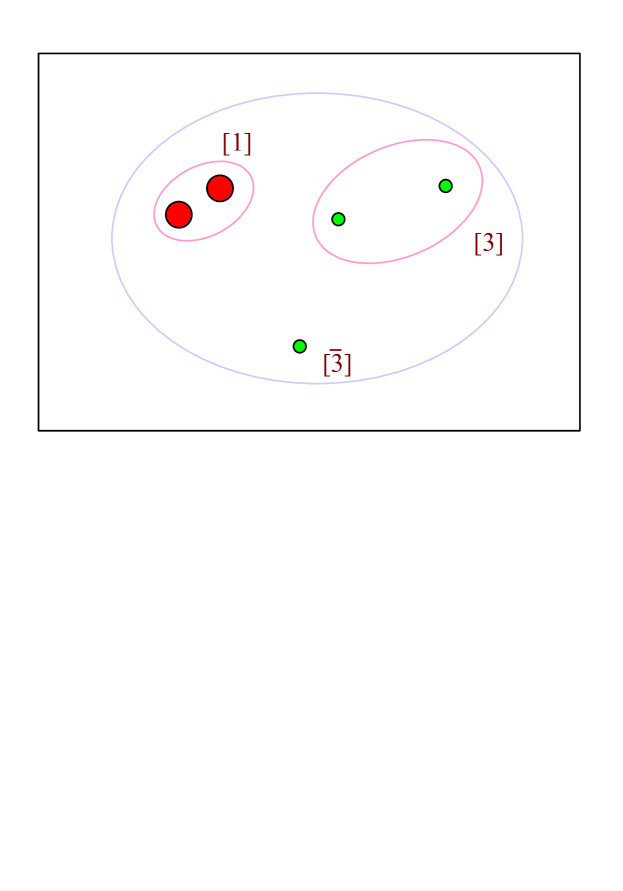
Figure 1: Color structure of a hidden-flavor pentaquark arising from the color Coulomb-like correlations between the heavy flavors. The large red circles stand for the heavy quark-antiquark pair, the small green circles represent the light quarks. The numbers between squared brackets denote the color wave function.

Taking into account that the heavy quarks have isospin zero and the antisymmetric character of the color-${\bf\bar{3}}$ $qq$ wave function – what implies that its spin and isospin must be identical – one can identify the different vectors that contribute to any $(I,J)$ pentaquark for the lowest lying states, i.e., in the case of a fully symmetric radial wave function,

$$\Psi^{(I,J)}_{\rm Pentaquark}\,\,=\,\,\{{\bf 3}_{c},i_{1}=1/2,s_{1}=1/2\}_{q}\,\otimes\,\{{\bf 1}_{c},i_{2}=0,s_{2}\}_{(Q\bar{Q})}\,\otimes\,\{{\bf\bar{3}}_{c},i_{3}=s_{3},s_{3}\}_{(qq)}\,.$$ (2)

We summarize in Table 1 the possible value of the quantum numbers leading to an allowed $(I,J)$ hidden-flavor pentaquark. $s_{1}$ stands for the spin of the single light quark (with isospin $1/2$), $s_{2}$ denotes the spin of the heavy quark-antiquark pair (with isospin zero) and finally $s_{3}$ represents the spin of the light quark pair (with the restrictions imposed by the Pauli principle such that $s_{3}=i_{3}$). The notation in the last column will be used in the next sections to identify the wave function of the different pentaquarks.

$I$		$J$		$s_{1}$		$s_{2}$		$s_{3}$		Vector
$1/2$		$1/2$		$1/2$		$0$		$0$		$v_{1}$
		$1/2$				$1$		$0$		$v_{2}$
		$1/2$				$0$		$1$		$v_{3}$
		$1/2$				$1$		$1$		$v_{4}$
		$3/2$				$1$		$0$		$w_{1}$
		$3/2$				$1$		$1$		$w_{2}$
		$5/2$				$1$		$1$		$y_{1}$
$3/2$		$1/2$		$1/2$		$1$		$1$		$v_{4}$
		$3/2$				$0$		$1$		$w_{3}$
		$3/2$				$1$		$1$		$w_{2}$
		$5/2$				$1$		$1$		$y_{1}$

Table 1: Quantum numbers of the different channels contributing to a given $(I,J)$ hidden-flavor pentaquark according to Eq. (2). See text for details.

Once the Hilbert space arising from the correlation between the heavy flavors has been delimited, the only ingredient left for our study is a realistic interaction between the quarks. In this paper we adopt a generic constituent model, containing chromoelectric and chromomagnetic contributions, tuned to reproduce the masses of the mesons and baryons entering the various vectors shown in Table 1. We adopt the so-called AL1 model by Semay and Silvestre-Brac Sem94 , widely used in a number of exploratory studies of multiquark systems Sil93 ; Ric18 ; Jan04 ; Her20 ; Ric17 ; Hiy18 ; Meg19 . It includes a standard Coulomb-plus-linear central potential, supplemented by a smeared version of the chromomagnetic interaction,

$$V(r) =-\frac{3}{16}\,\tilde{\lambda}_{i}.\tilde{\lambda}_{j}\left[\lambda\,r-\frac{\kappa}{r}-\Lambda+\frac{V_{SS}(r)}{m_{i}\,m_{j}}\,\vec{\sigma}_{i}\cdot\vec{\sigma}_{j}\right]\,,$$ (3)

$$V_{SS} =\frac{2\,\pi\,\kappa^{\prime}}{3\,\pi^{3/2}\,r_{0}^{3}}\,\exp\left(-\frac{r^{2}}{r_{0}^{2}}\right)~{},\quad r_{0}=A\left(\frac{2m_{i}m_{j}}{m_{i}+m_{j}}\right)^{-B}\,,$$

where $\lambda=$ 0.1653 GeV², $\Lambda=$ 0.8321 GeV, $\kappa=$ 0.5069, $\kappa^{\prime}=$ 1.8609, $A=$ 1.6553 GeV^B-1, $B=$ 0.2204, $m_{u}=m_{d}=$ 0.315 GeV, $m_{s}=$ 0.577 GeV, $m_{c}=$ 1.836 GeV and $m_{b}=$ 5.227 GeV. Here, $\tilde{\lambda}_{i}.\tilde{\lambda}_{j}$ is a color factor, suitably modified for the quark-antiquark pairs. Note that the smearing parameter of the spin-spin term is adapted to the masses involved in the quark-quark or quark-antiquark pairs. The parameters of the AL1 potential are constrained in a simultaneous fit of 36 well-established mesons and 53 baryons, with a remarkable agreement with data, as could be seen in Table 2 of Ref. Sem94 . It is worth to note that although the $\chi^{2}$ obtained in Ref. Sem94 with the AL1 potential is slightly larger than the one obtained with other models, this is essentially because a number of resonances with high angular momenta were considered. The AL1 model is very well suited to study the low-energy hadron spectra Sil96 . The spin-color algebra of the five-quark system has been worked elsewhere Ale11 ; Ric17 . The capability of the model to describe relevant ordinary hadrons: $Q\bar{Q}$, $q\bar{Q}$, $qqq$ and $Qqq$, is illustrated in Table 2 for $Q=c$.

Baryons						Mesons
State		AL1		Exp.		State		AL1		Exp.
$N$		996		940		$D$		1862		1868
$\Delta$		1307		1232		$D^{*}$		2016		2008
$\Lambda_{c}$		2292		2286		$\eta_{c}$		3005		2989
$\Sigma_{c}$		2467		2455		$J/\psi$		3101		3097
$\Sigma^{*}_{c}$		2546		2518

Table 2: Masses (in MeV) of ordinary hadrons calculated with the AL1 potential of Eq. (3), compared to the experimental values.

The bound nature of a multiquark could arise from an attractive medium-long range interaction generated by the exchange of color-singlet Goldstone bosons Vij04 ; Hua16 ; Yan17 . In addition, it is known that the short-range one-gluon exchange interaction generates a strong repulsive force in the $NN$ $S$-wave partial waves. This feature is not universal for a hadron-hadron interaction in general. Indeed, it disappears for some channels of, among others, the $\Delta\Delta$ and $N\Delta$ systems, generating a positive phase shift at low energies Oka80 . This attractive short-range behavior was the basis of resonances predicted in the $\Delta\Delta$ and $N\Delta$ systems Gol89 ; Pan01 ; Mot99 ; Val01 , some of which have been established experimentally Cle17 . Thus, the short-range quark-gluon dynamics of multiquark systems may also induce stability.

Let us finally note that once the color wave function is frozen by the dynamical correlations between the heavy flavors and being all the constituents spin $1/2$ particles, the flavor-independence of the interacting potential makes the five-body problem to factorize into the three-body problem shown in Fig. 1. The existence of correlated substructures in a many-quark system leads, in general, to more tractable technical problems. This is for instance the case of tetraquark studies under the diquark hypothesis Kar17 ; Eic17 , where the four-body problem is reduced to a two-body problem of effective diquarks with a mass fixed in other known hadron sectors. In the problem addressed in this manuscript, the correlations between the heavy flavors leads to a three-body problem that can be exactly solved by means of the Faddeev equations. This also allows to overcome the difficulties associated to the minimization procedure inherent to variational methods for getting fully converged results. This is particularly relevant working close to open thresholds. We discuss in the next section the solution of the Faddeev equations for the bound state problem of a three-body system.

III The three-body problem

The freezing of the color wave function described in the previous section leads to the effective three-body problem shown in Fig. 1 and summarized in the wave function of Eq. (2). The allowed spin and isospin values of the different particles – $1$: light quark, $2$: heavy quark-antiquark pair, $3$: two light-quark pair – are indicated in Table 1.

Table 3: Channels that are coupled together for the different $J=1/2$ states, $v_{i}$ in Table 1. See text for details.

		$s_{1}$		$s_{2}$		$S_{3}$		$s_{3}$		$I$		$F$
$v_{1}$		$1/2$		$0$		$1/2$		$0$		$1/2$		$9/8$
$v_{2}$		$1/2$		$1$		$1/2$		$0$		$1/2$		$3/8$
$v_{3}$		$1/2$		$0$		$1/2$		$1$		$1/2$		$9/8$
$v_{4}$		$1/2$		$1$		$1/2$		$1$		$1/2,3/2$		$3/8$
		$1/2$		$1$		$3/2$		$1$		$1/2,3/2$		$3/2\sqrt{2}$
		$s_{2}$		$s_{3}$		$S_{1}$		$s_{1}$
$v_{1}$		$0$		$0$		$0$		$1/2$		$1/2$		$0$
$v_{2}$		$1$		$0$		$1$		$1/2$		$1/2$		$0$
$v_{3}$		$0$		$1$		$1$		$1/2$		$1/2$		$0$
$v_{4}$		$1$		$1$		$0$		$1/2$		$1/2,3/2$		$-4/3$
		$1$		$1$		$1$		$1/2$		$1/2,3/2$		$-5/3$
		$s_{3}$		$s_{1}$		$S_{2}$		$s_{2}$
$v_{1}$		$0$		$1/2$		$1/2$		$0$		$1/2$		$9/8$
$v_{2}$		$0$		$1/2$		$1/2$		$1$		$1/2$		$9/8$
$v_{3}$		$1$		$1/2$		$1/2$		$0$		$1/2$		$3/8$
$v_{4}$		$1$		$1/2$		$1/2$		$1$		$1/2,3/2$		$3/8$
		$1$		$1/2$		$3/2$		$1$		$1/2,3/2$		$3/2\sqrt{2}$

Table 4: Same as Table 3 for $J=3/2$ states, $w_{i}$ in Table 1.

		$s_{1}$		$s_{2}$		$S_{3}$		$s_{3}$		$I$		$F$
$w_{1}$		$1/2$		$1$		$3/2$		$0$		$1/2$		$3/2\sqrt{2}$
$w_{2}$		$1/2$		$1$		$1/2$		$1$		$1/2,3/2$		$3/8$
		$1/2$		$1$		$3/2$		$1$		$1/2,3/2$		$3/2\sqrt{2}$
$w_{3}$		$1/2$		$0$		$1/2$		$1$		$3/2$		$9/8$
		$s_{2}$		$s_{3}$		$S_{1}$		$s_{1}$
$w_{1}$		$1$		$0$		$1$		$1/2$		$1/2$		$0$
$w_{2}$		$1$		$1$		$1$		$1/2$		$1/2,3/2$		$2/3$
		$1$		$1$		$2$		$1/2$		$1/2,3/2$		$-2/3$
$w_{3}$		$0$		$1$		$1$		$1/2$		$3/2$		$0$
		$s_{3}$		$s_{1}$		$S_{2}$		$s_{2}$
$w_{1}$		$0$		$1/2$		$1/2$		$1$		$1/2$		$9/8$
$w_{2}$		$1$		$1/2$		$1/2$		$1$		$1/2,3/2$		$3/8$
		$1$		$1/2$		$3/2$		$1$		$1/2,3/2$		$3/2\sqrt{2}$
$w_{3}$		$1$		$1/2$		$3/2$		$0$		$3/2$		$3/2\sqrt{2}$

Table 5: Same as Table 3 for $J=5/2$ states, $y_{i}$ in Table 1.

		$s_{1}$		$s_{2}$		$S_{3}$		$s_{3}$		$I$		$F$
$y_{1}$		$1/2$		$1$		$3/2$		$1$		$1/2,3/2$		$3/2\sqrt{2}$
		$s_{2}$		$s_{3}$		$S_{1}$		$s_{1}$
$y_{1}$		$1$		$1$		$2$		$1/2$		$1/2,3/2$		$1$
		$s_{3}$		$s_{1}$		$S_{2}$		$s_{2}$
$y_{1}$		$1$		$1/2$		$3/2$		$1$		$1/2,3/2$		$3/2\sqrt{2}$

Three-body states in which a particle has a given spin can only couple to other three-body states in which that particle has the same spin, since the spinors corresponding to different eigenvalues are orthogonal. This is shown in detail in Appendix A. The same applies for isospin. This leads to a decoupling of the integral equations in various sets in which the spin and isospin of each particle remains the same. We show the different sets contributing to $J=1/2$, $3/2$, and $5/2$ in Tables 3, 4, and 5, respectively. Besides the notation introduced in Table 1, we denote by $S_{i}$ and $I_{i}$ the spin and isospin of the pair $jk$. As discussed above, the isospin of each particle is determined once the spin is given, so it is not shown in the tables. Finally, $F$ is the expectation value of the $\vec{\sigma}_{i}\cdot\vec{\sigma}_{j}$ operator, responsible for the coupling of different two-body amplitudes as explained below.

To solve the Faddeev equations in momentum space for the case of confining potentials we follow the method developed in Ref. Gar03 , that it is described below for $S$- and $P$-wave states.

III.1 $S$-wave states

We restrict ourselves to the configurations where all three particles are in $S$-wave states so that the Faddeev equations for the bound-state problem with total isospin $I$ and total spin $J$ are,

$$T_{i;IJ}^{I_{i}S_{i}}(p_{i}q_{i})= \sum_{j\neq i}\sum_{I_{j}S_{j}}\frac{1}{2}\int_{0}^{\infty}q_{j}^{2}dq_{j}\int_{-1}^{1}d{\rm cos}\theta\,t_{i;I_{i}S_{i}}(p_{i},p_{i}^{\prime};E-q_{i}^{2}/2\nu_{i})$$ (4)

$$\times\,h_{ij;IJ}^{I_{i}S_{i};I_{j}S_{j}}\frac{1}{E-p_{j}^{2}/2\eta_{j}-q_{j}^{2}/2\nu_{j}}\;T_{j;IJ}^{I_{j}S_{j}}(p_{j}q_{j})\,,$$

where $t_{i;I_{i}S_{i}}$ stands for the two-body amplitudes with isospin $I_{i}$ and spin $S_{i}$ and $\eta_{i}$ and $\nu_{i}$ are the corresponding reduced masses,

$$\eta_{i} = \frac{m_{j}m_{k}}{m_{j}+m_{k}}\,,$$

$$\nu_{i} = \frac{m_{i}(m_{j}+m_{k})}{m_{i}+m_{j}+m_{k}}\,,$$ (5)

$\vec{p}_{i}^{\;\prime}$ is the momentum of the pair $jk$ (with $ijk$ an even permutation of $123$) and $\vec{p}_{j}$ is the momentum of the pair $ki$ which are given by,

$$\vec{p}_{i}^{\;\prime} = -\vec{q}_{j}-\alpha_{ij}\vec{q}_{i}\,,$$

$$\vec{p}_{j} = \vec{q}_{i}+\alpha_{ji}\vec{q}_{j}\,,$$ (6)

where,

$$\alpha_{ij} = \frac{\eta_{i}}{m_{k}}\,,$$

$$\alpha_{ji} = \frac{\eta_{j}}{m_{k}}\,,$$ (7)

so that,

$$p_{i}^{\prime} = \sqrt{q_{j}^{2}+\alpha_{ij}^{2}q_{i}^{2}+2\alpha_{ij}q_{i}q_{j}{\rm cos}\theta}\,,$$

$$p_{j} = \sqrt{q_{i}^{2}+\alpha_{ji}^{2}q_{j}^{2}+2\alpha_{ji}q_{i}q_{j}{\rm cos}\theta}\,.$$ (8)

$h_{ij;IJ}^{I_{i}S_{i};I_{j}S_{j}}$ are the spin–isospin coefficients,

$$h_{ij;IJ}^{I_{i}S_{i};I_{j}S_{j}}= (-)^{I_{j}+i_{j}-I}\sqrt{(2I_{i}+1)(2I_{j}+1)}W(i_{j}i_{k}Ii_{i};I_{i}I_{j})$$ (9)

$$\times(-)^{S_{j}+s_{j}-J}\sqrt{(2S_{i}+1)(2S_{j}+1)}W(s_{j}s_{k}Js_{i};S_{i}S_{j})\,,$$

where $W$ is a Racah coefficient and $i_{i}$, $I_{i}$, and $I$ ($s_{i}$, $S_{i}$, and $J$) are the isospins (spins) of particle $i$, of the pair $jk$, and of the three–body system.

In Eq. (4) the variable $p_{i}$ runs from 0 to $\infty$. Thus, it is convenient to make the transformation,

$$x_{i}=\frac{p_{i}-b}{p_{i}+b}\,,$$ (10)

where the new variable $x_{i}$ runs from $-1$ to $1$, and $b$ is a scale parameter that has no effect on the solution. With this transformation Eq. (4) takes the form,

$$T_{i;IJ}^{I_{i}S_{i}}(x_{i}q_{i})= \sum_{j\neq i}\sum_{I_{j}S_{j}}\frac{1}{2}\int_{0}^{\infty}q_{j}^{2}dq_{j}\int_{-1}^{1}d{\rm cos}\theta\;t_{i;I_{i}S_{i}}(x_{i},x_{i}^{\prime};E-q_{i}^{2}/2\nu_{i})$$ (11)

$$\times\,h_{ij;IJ}^{I_{i}S_{i};I_{j}S_{j}}\frac{1}{E-p_{j}^{2}/2\eta_{j}-q_{j}^{2}/2\nu_{j}}\;T_{j;IJ}^{I_{j}S_{j}}(x_{j}q_{j})\,.$$

Since the variables $x_{i}$ and $x_{i}^{\prime}$ run from $-1$ to $1$, one can expand the amplitude $t_{i;I_{i}S_{i}}(x_{i},x_{i}^{\prime};e)$ in terms of Legendre polynomials as,

$$t_{i;I_{i}S_{i}}(x_{i},x_{i}^{\prime};e)=\sum_{nr}P_{n}(x_{i})\tau_{i;I_{i}S_{i}}^{nr}(e)P_{r}(x^{\prime}_{i})\,,$$ (12)

where the expansion coefficients are given by,

$$\tau_{i;I_{i}S_{i}}^{nr}(e)=\frac{2n+1}{2}\frac{2r+1}{2}\int_{-1}^{1}dx_{i}\int_{-1}^{1}dx_{i}^{\prime}\;P_{n}(x_{i})t_{i;I_{i}S_{i}}(x_{i},x_{i}^{\prime};e)P_{r}(x_{i}^{\prime})\,.$$ (13)

Applying expansion (12) in Eq. (11) one gets,

$$T_{i;IJ}^{I_{i}S_{i}}(x_{i}q_{i})=\sum_{n}P_{n}(x_{i})T_{i;IJ}^{nI_{i}S_{i}}(q_{i})\,,$$ (14)

where $T_{i;IJ}^{nI_{i}S_{i}}(q_{i})$ satisfies the one-dimensional integral equation,

$$T_{i;IJ}^{nI_{i}S_{i}}(q_{i})=\sum_{j\neq i}\sum_{mI_{j}S_{j}}\int_{0}^{\infty}dq_{j}K_{ij;IJ}^{nI_{i}S_{i};mI_{j}S_{j}}(q_{i},q_{j};E)\;T_{j;IJ}^{mI_{j}S_{j}}(q_{j})\,,$$ (15)

with

$$K_{ij;IJ}^{nI_{i}S_{i};mI_{j}S_{j}}(q_{i},q_{j};E)= \sum_{r}\tau_{i;I_{i}S_{i}}^{nr}(E-q_{i}^{2}/2\nu_{i})\frac{q_{j}^{2}}{2}$$ (16)

$$\times\int_{-1}^{1}d{\rm cos}\theta\;h_{ij;IJ}^{I_{i}S_{i};I_{j}S_{j}}\frac{P_{r}(x_{i}^{\prime})P_{m}(x_{j})}{E-p_{j}^{2}/2\eta_{j}-q_{j}^{2}/2\nu_{j}}\,.$$

The three amplitudes $T_{1;IJ}^{rI_{1}S_{1}}(q_{1})$, $T_{2;IJ}^{mI_{2}S_{2}}(q_{2})$, and $T_{3;IJ}^{nI_{3}S_{3}}(q_{3})$ in Eq. (15) are coupled together.

III.2 $P$-wave states

In all the previous sets of coupled equations we have assumed only $S$-wave states. We thought interesting, however, to look into excited states containing one unit of orbital angular momentum. For that purpose we have chosen the state $v_{1}$ in Table 1, where $s_{2}=s_{3}=0$. We show in Table 6 the two-body channels that are coupled together in this case. $\ell_{i}$ is the relative orbital angular momentum of the pair $jk$ and $\lambda_{i}$ is the relative orbital angular momentum between particle $i$ and the pair $jk$.

Table 6: Channels that are coupled together for the vector $v_{1}$ in Table 1 with a unit of orbital angular momentum, such that $J=1/2$ and $3/2$.

		$s_{1}$		$s_{2}$		$S_{3}$		$s_{3}$		$\ell_{3}$		$\lambda_{3}$		$I$		$F$
$v_{1}$		$1/2$		$0$		$1/2$		$0$		$0$		$1$		$1/2$		$9/8$
		$1/2$		$0$		$1/2$		$0$		$1$		$0$		$1/2$		$9/8$
		$s_{2}$		$s_{3}$		$S_{1}$		$s_{1}$		$\ell_{1}$		$\lambda_{1}$		$I$		$F$
$v_{1}$		$0$		$0$		$0$		$1/2$		$0$		$1$		$1/2$		$0$
		$0$		$0$		$0$		$1/2$		$1$		$0$		$1/2$		$0$
		$s_{3}$		$s_{1}$		$S_{2}$		$s_{2}$		$\ell_{2}$		$\lambda_{2}$		$I$		$F$
$v_{1}$		$0$		$1/2$		$1/2$		$0$		$0$		$1$		$1/2$		$9/8$
		$0$		$1/2$		$1/2$		$0$		$1$		$0$		$1/2$		$9/8$

To solve the integral equations (4) with one unit of orbital angular momentum we write them symbolically as,

$$T_{i}=t_{i}h_{ij}G_{0}T_{j},$$ (17)

that has to be generalized to a matrix equation,

$$\begin{pmatrix}T_{i}^{01}\\ T_{i}^{10}\end{pmatrix}=\begin{pmatrix}t_{i}^{0}\\ t_{i}^{1}\end{pmatrix}h_{ij}G_{0}\begin{pmatrix}\hat{q}_{i}\cdot\hat{q}_{j}&\hat{q}_{i}\cdot\hat{p}_{j}\\ \hat{p}_{i}^{\;\prime}\cdot\hat{q}_{j}&\hat{p}_{i}^{\;\prime}\cdot\hat{p}_{j}\end{pmatrix}\begin{pmatrix}T_{j}^{01}\\ T_{j}^{10}\end{pmatrix},$$ (18)

where, from Eq. (6),

$$\hat{q}_{i}\cdot\hat{q}_{j} = {\rm cos}\theta\,,$$

$$\hat{q}_{i}\cdot\hat{p}_{j} = \frac{q_{i}^{2}+\alpha_{ji}q_{i}q_{j}{\rm cos}\theta}{q_{i}p_{j}}\,,$$

$$\hat{p}_{i}^{\;\prime}\cdot\hat{q}_{j} = \frac{-q_{j}^{2}-\alpha_{ij}q_{i}q_{j}{\rm cos}\theta}{p_{i}^{\prime}q_{j}}\,,$$

$$\hat{p}_{i}^{\;\prime}\cdot\hat{p}_{j} = \frac{-(1+\alpha_{ij}\alpha_{ji})q_{i}q_{j}{\rm cos}\theta-\alpha_{ji}q_{j}^{2}-\alpha_{ij}q_{i}^{2}}{p_{i}^{\prime}p_{j}}\,,$$ (19)

and $p_{i}^{\prime}$ and $p_{j}$ are given by Eq. (8).

III.3 Coupling between two-body amplitudes

In general, the two-body amplitudes that appear in Tables 3, 4, 5, and 6 are obtained by solving the Lippmann-Schwinger equation,

$$t=V+VG_{0}t\,,$$ (20)

where $V$ is the interaction given by Eq. (3). Due to the reduction from five to three particles, some pairs of two-body amplitudes are coupled together. Such is the case of the $S_{1}=0$ and $S_{1}=1$ amplitudes of the $v_{4}$ vector in Table 3, which are coupled by the chromomagnetic term of the interacting potential. Therefore, in this case one has to solve the coupled equations,

$$t_{11} = V_{11}+V_{11}G_{0}t_{11}+V_{12}G_{0}t_{21}\,,$$

$$t_{21} = V_{21}+V_{21}G_{0}t_{11}+V_{22}G_{0}t_{21}\,,$$ (21)

where the diagonal interactions $V_{11}$ and $V_{22}$ show contributions from the chromoelectric and chromomagnetic terms of the interaction, while the off-diagonal interactions $V_{12}$ and $V_{21}$ contain only the contribution of the chromomagnetic part of the interacting potential. As expected, the confinement and Coulomb terms are the dominant ones such that the spin-spin term is just a small perturbation. The effect of the non-diagonal terms is very small and it can be safely neglected.

IV Results

We have solved the three-body problem for the different $(I,J)$ states as discussed in Sec. III by taking $m_{1}=m_{u,d}$, $m_{2}=2m_{c}$ and $m_{3}=2m_{u,d}$.  We show in Fig. 2 the five-quark states that are below threshold. Regarding the isospin 1/2 states, left panel, they are organized in two different shells. The lowest band contains $J=1/2$ and $3/2$ states with the two-quark subclusters with maximum spin. It is worth to note that in the two-baryon system the one-gluon exchange also generates the larger attraction for parallel spin configurations Oka80 ; Gol89 ; Pan01 ; Mot99 ; Val01 . Some states are rather close in energy and therefore hard to distinguish experimentally. In the upper shell there appear states with $J=1/2$, $3/2$ and $5/2$. The $J=5/2$ state is at threshold. Right panel on Fig. 2 shows the spectra of the isospin $3/2$ states.

Let us first note the degeneracy existing between $I=1/2$ and $I=3/2$ states, as could have been expected a priori due to the isospin independence of the potential model in Eq. (3), although the result is not trivial due to the requirements of the Pauli principle. Secondly, it has been checked that the conclusions dealing with stability or instability of multiquarks survive variations of the parameters, we have specifically checked that the pattern remains for different strengths of the spin-spin interaction by modifying the regularization parameter, $r_{0}$ in Eq. (3).

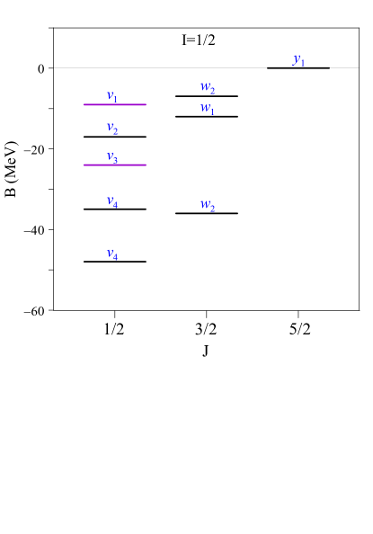
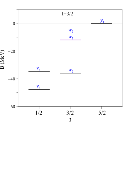
Figure 2: Binding energy, in MeV, for the different hidden-charm pentaquarks. Black lines stand for states containing a spin one heavy quark-antiquark pair and purple lines denote states with a spin zero heavy quark-antiquark pair. The corresponding vector of Table 1 is indicated in the figure. Left panel: $I=1/2$. Right panel: $I=3/2$.

There are additional quark correlations dominating the QCD phenomena Jaf05 that could hint to the most favorable states that can be observed in nature. First, the very strong quark-antiquark correlation in the color-, flavor-, and spin-singlet channel $\{{\bf 1}_{c},{\bf 1}_{f},0_{s}\}$ which can be viewed as the responsible for chiral symmetry breaking. The attractive forces in this channel are so strong that condenses in the vacuum, breaking $SU(N_{f})_{L}\times SU(N_{f})_{R}$ chiral symmetry. The next most attractive channel in QCD seems to be the color antitriplet, flavor antisymmetric, spin singlet $\{{\bf\bar{3}}_{c},{\bf\bar{3}}_{f},0_{s}\}$, that would select the $qq$ configurations most important spectroscopically. Thus, we show in Fig. 3 the resulting spectrum by selecting those states that contain at least one the most attractive QCD channels, i.e., a diquark with spin zero. It is observed that the $J=5/2$ state at threshold disappears as well as the pentaquarks of the lowest shell.

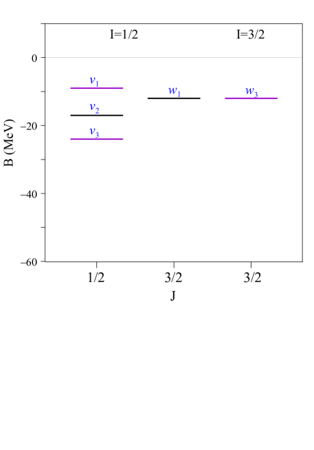
Figure 3: $I=1/2$ and $3/2$ hidden-charm pentaquarks containing substructures dictated by the quark correlations dominating the QCD phenomena Jaf05 . The notation is the same as in Fig. 2.

The general properties of the multiquarks favored by the quark correlations dominating the QCD phenomena shown in Fig. 3 can be easily estimated. In the charmonium sector, the mass difference between the $Q\bar{Q}$ $\{{\bf 1}_{c},{\bf 1}_{f},1_{s}\}$ and $\{{\bf 1}_{c},{\bf 1}_{f},0_{s}\}$ correlated states could be assimilated to the $J/\Psi-\eta_{c}$ mass difference. The mass difference between the $qq$ $\{{\bf\bar{3}}_{c},{\bf 6}_{f},1_{s}\}$ and $\{{\bf\bar{3}}_{c},{\bf\bar{3}}_{f},0_{s}\}$ has been estimated from full lattice QCD simulations to be in the range of 100$-$200 MeV Fra21 ; Ale06 ; Gre10 . We have tuned the effective masses of the correlated structures to the hidden-charm pentaquarks, considering the following realistic values,

$$\Delta M^{Q\bar{Q}}=M^{Q\bar{Q}}_{\{{\bf 1}_{c},{\bf 1}_{f},1_{s}\}}-M^{Q\bar{Q}}_{\{{\bf 1}_{c},{\bf 1}_{f},0_{s}\}} =86\,\,{\rm MeV}\,,$$

$$\Delta M^{qq}=M^{qq}_{\{{\bf\bar{3}}_{c},{\bf 6}_{f},1_{s}\}}-M^{qq}_{\{{\bf\bar{3}}_{c},{\bf\bar{3}}_{f},0_{s}\}} =146\,\,{\rm MeV}\,.$$ (22)

Thus, denoting by $M_{0}$ the sum of the masses of a spin zero $Q\bar{Q}$ diquark, a spin zero $qq$ diquark and a light quark, the mass of the states shown in Fig. 3 would be given by

$$M_{i}=M_{0}-B_{i}+\Delta M^{Q\bar{Q}}\,\delta_{s_{2},1}+\Delta M^{qq}\,\delta_{s_{3},1}\,,$$ (23)

where $B_{i}$ is the binding energy calculated above. By taking $M_{0}=4321$ MeV, one gets the results shown in Table 7.

Vector		$(I)J^{P}$		$M_{\rm Th}$ (MeV)		State		$M_{\rm Exp}$ (MeV)
$v_{1}$		$(1/2)1/2^{-}$		4312		$P_{c}(4312)^{+}$		$4311.9\pm 0.7^{+6.8}_{-0.6}$
$v_{2}$		$(1/2)1/2^{-}$		4390		$P_{c}(4380)^{+}$		$4380\pm 8\pm 29$
$w_{1}$		$(1/2)3/2^{-}$		4395
$v_{3}$		$(1/2)1/2^{-}$		4443		$P_{c}(4440)^{+}$		$4440.3\pm 1.3^{+4.1}_{-4.7}$
$w_{3}$		$(3/2)3/2^{-}$		4455		$P_{c}(4457)^{+}$		$4457.3\pm 0.6^{+4.1}_{-1.7}$

Table 7: Properties of the hidden-charm pentaquarks of Fig. 3.

As can be seen, there is a good agreement between theoretical states showing the most important correlations dictated by the QCD phenomena and the experimental data Aai15 ; Aai19 . Thus, Table 7 presents a theoretical spin-parity assignment for the existing hidden-charm pentaquarks.

The spin-parities of the hidden-charm pentaquarks are not yet determined Bra20 . Nevertheless, there are predictions based on different models that can be compared with. Although there are different proposals about the $P_{c}(4312)^{+}$ quantum numbers Zhu16 , there seems to be a general preference for $J^{P}=1/2^{-}$ Wun10 ; Wan11 ; Yan12 ; Wul12 ; Xia13 ; Yaa17 , as it is found in our model. The two narrow overlapping structures, $P_{c}(4440)^{+}$ and $P_{c}(4457)^{+}$ Aai19 , were originally reported as a single state, $P_{c}(4450)^{+}$ Aai15 . There were earlier predictions of two almost degenerate states with $J^{P}=1/2^{-}$ and $3/2^{-}$ at the position of the $P_{c}(4450)^{+}$ pentaquark. These structures corresponded to the $J^{P}=1/2^{-}$ and $3/2^{-}$ hidden-charm states created dynamically by the $\Sigma_{c}\bar{D}^{*}$ charmed meson-baryon interactions Wun10 ; Wum11 ; Xia13 . They were also predicted as bound states of charmonium $\Psi(2S)$ and the nucleon Eid16 . In both cases the quantum numbers of the $P_{c}(4440)^{+}$ and $P_{c}(4457)^{+}$ pentaquarks agree with our findings. Finally, in our model there are two theoretical candidates, one with $J=1/2$ and the other with $J=3/2$, for the $P_{c}(4380)^{+}$, a wide resonance whose nature is still an intriguing issue and is an outstanding challenge for future experiments Kar15 . The preferred spin assignment for this state was $J=3/2$ or $5/2$ Aai15 . A recent analysis of $B_{s}\to J/\Psi p\bar{p}$ decays supports a $J^{P}=3/2^{-}$ assignment Wag21 . Thus, we could assign the $P_{c}(4380)^{+}$ to the $J^{P}=3/2^{-}$ state of our model and therefore leaving open the existence of another $J^{P}=1/2^{-}$ pentaquark in the same energy region, with a mass of about 4390 MeV.

Preliminary analysis of the experimental data suggested the coexistence of negative and positive parity pentaquarks in the same energy region Aai15 . We have studied such possibility within our model. For this purpose, we have calculated the mass of the lowest positive parity state, the first orbital angular momentum excitation of the $v_{1}$ state. The technical details have been described in Sec. III.2. We chose this state because it is made up of the most strongly correlated structures, $Q\bar{Q}$ $\{{\bf 1}_{c},{\bf 1}_{f},0_{s}\}$ and $qq$ $\{{\bf\bar{3}}_{c},{\bf\bar{3}}_{f},0_{s}\}$. Then, it might have a similar mass to negative parity states made up of spin 1 structures. We have obtained an energy of 197 MeV above threshold. By using the values given in Eq. (IV) one obtains a mass of 4518 MeV for two degenerate states with quantum numbers $J^{P}=1/2^{+}$ and $3/2^{+}$. Therefore, positive parity pentaquark states would appear above 4.5 GeV, a mass slightly larger than that of the states measured so far. Similarly, most of the theoretical works prefer to assign the lowest lying pentaquarks to negative parity states. Almost degenerate negative and positive parity states may occur for hidden-flavor pentaquarks that have been detected in the same channel but that were formed by different pairs of quarkonium-nucleon states Eid16 , one of them radially excited. Thus the negative parity pentaquark of the $(Q\bar{Q})_{n+1,S}(qqq)$ system would have a similar mass than the positive parity orbital angular momentum excited state of the $(Q\bar{Q})_{n,S}(qqq)$ system. The assignment of negative and positive parity states to different parity Born-Oppenheimer multiplets has already been suggested as a plausible solution in the triquark-diquark picture of Ref. Gir19 . Nevertheless, this issue remains one of the most challenging problems in the pentaquark phenomenology that should be first confirmed experimentally.

Multiquark states would show very different decay patterns regarding its internal structure Wul17 . The decays of the pentaquarks in Table 7 into an (anti)charmed meson + charmed baryon are strongly suppressed since decays into open charm channels can go only via $t$-channel exchange by a heavy $D$ meson. Due to the content of the pentaquarks states they would follow the decays of charmonium excited states, $\Psi(nS)$ and $\eta_{c}(nS)$. Thus, multiquarks containing a spin zero heavy quark-antiquark pair: $v_{1}$, $v_{3}$ and $w_{3}$ in Table 7, would be narrower than those with a spin one heavy quark-antiquark pair: $v_{2}$ and $w_{1}$ in Table 7. This corresponds nicely with the experimental observations. However, besides the contribution to the width of the substructures that form each pentaquark, one should also consider the width due to the bound nature of the system. At this point it is worth to mention that the final width of a resonance does not come only determined by its internal content, but there are significant corrections due to an interplay between the phase space for its decay to the detection channel and its mass with respect to the hadrons generating the state Gar18 .

The existence of hidden-flavor pentaquarks has been concluded in various constituent quark-model studies. Let us analyze our results compared to other related approaches in the literature. Ref. Hua16 studies hidden-charm pentaquarks in a quark delocalization color screening model, where besides the one-gluon exchange potential quarks interact through the exchange of Goldstone bosons. It presents results for $I=1/2$ pentaquarks concluding the existence of several negative parity bound states with $J=1/2$, $3/2$, and $5/2$. The lowest state corresponds to $J=1/2$ and the $J=5/2$ state is at the edge of binding. The deepest states with $J=1/2$ and J=$3/2$ are found in the $(Q\bar{Q})(qqq)$ configuration. This is the structure favored by the color Coulomb-like short-range correlations between the heavy flavors. In fact, the $(q\bar{Q})(Qqq)$ configuration only shows quasi-stable states that should be confirmed by investigating the scattering process of other open channels. The results are in good agreement with the $I=1/2$ results of our model, the deepest state being $J=1/2$ while the only $J=5/2$ state is at threshold. These findings come to give support to the existence of a color-singlet correlation between the heavy flavors within the pentaquarks.

Ref. Yan17 discusses results for $I=1/2$ states based on a chiral-quark model. Several negative parity bound states with $J=1/2$, $3/2$, and $5/2$ are reported. In contrast to Ref. Hua16 the dominant configuration is found to be $(q\bar{Q})(Qqq)$. It may be because in the $(Q\bar{Q})(qqq)$ configuration, quarkonium and baryons do not share light $u$ and $d$ quarks and thus the OZI rule suppresses the interactions mediated by the exchange of mesons made of only light quarks Bro90 . The exchange of $D$ mesons is a too short-range interaction to compete with the medium-range attraction that can be generated by light-meson exchanges arising in the $(q\bar{Q})(Qqq)$ configuration. It is also worth to note that hybrid models containing gluon and meson exchanges at quark level show a reduced strength of the one-gluon exchange potential Vij04 . This is because pseudoscalar meson exchanges between quarks do also contribute to the $\Delta-N$ mass difference. However, the pseudoscalar spin-flavor interaction favors different color-spin components than those favored by the one-gluon exchange Val97 . As a consequence, a distinct pattern of multiquark states is found in hybrid or pure one-gluon exchange approaches.

Different studies concluded the existence of $I=3/2$ pentaquarks. In the so-called hadroquarkonium approach, Ref. Per16 presents robust predictions of isospin $3/2$ bound states of $\Psi(2S)$ and $\Delta$ with masses around 4.5 GeV. Looking back to constituent quark approaches, Ref. Ric17 concluded the existence of $I=3/2$ hidden-flavor pentaquarks. The pattern obtained is rather similar to our calculation, with the $J=5/2$ state being almost at threshold (note that we only consider relative $S$ waves). Regarding the $I=1/2$ states, it is the presence of the $(q\bar{Q})(Qqq)$ configuration, in other words repulsive color octets in the $(Q\bar{Q})(qqq)$ configuration, which rules out the possibility of having bound states. Therefore, the dynamical correlations arising among the heavy flavors are more effective for isospin $1/2$ states. This is easily understandable due to the fully symmetric nature of the isospin $3/2$ wave function, which in itself reduces the allowed Hilbert space vectors.

Ref. Wul17 studies hidden-flavor pentaquarks using the more repulsive color octet-color octet component, ${\bf 8}_{(Q\bar{Q})}{\bf 8}_{(qqq)}$. A set of negative parity states that would remain bound only against the heavier $(q\bar{Q})(Qqq)$ threshold is reported. The most distinctive feature of this approach lies in the fact that compact pentaquarks with a colored $qqq$ cluster have small branching ratios for the hidden-flavor decay channels as compared to possible baryon-meson molecules.

Ref. Wen19 makes use of an extended chromomagnetic model where besides the color-spin chromomagnetic potential, effective quark-pair mass parameters accounting for the effective quark masses and the color interaction between two quarks are considered. These parameters are fitted to the meson and baryon spectra. 10 $I=1/2$ and 7 $I=3/2$ hidden-flavor pentaquarks are found. All of them are negative parity states and there appear $J=1/2$, $3/2$ and $5/2$ pentaquarks in both isospin channels. The pattern of $I=1/2$ states shown in Fig. 1 of Ref. Wen19 is similar to our results. However, the degeneracy between $I=1/2$ and $I=3/2$ states is not observed in the spectra. This could be due to the way the effective quark-pair mass parameters are determined, because the interacting potential is isospin independent.

In addition to the models we have discussed with which the comparison is meaningful since they follow a similar constituent approach, as mentioned in the introduction, there are different proposals used to study hidden-flavor pentaquarks. The predictions of diquark models are very varied Mai15 ; Gir19 ; Ali19 ; Shi21 , depending on the hypotheses used for the diquark dynamics. Some further assumptions are sometimes made about the chromomagnetic interaction between diquarks Mai14 . A similar general conclusion can be derived from QCD sum rules studies, where one can find either molecular approaches Zha19 ; Che19 ; Azi17 ; Wan21 or others based on hidden-color components Pim20 . A recent review about the status of heavy quark sum rules and the uses for exotic hadron molecules can be found in Ref. Nar21 . Hadronic molecular models based either on effective chiral Lagrangians or one-boson exchange potentials rely on the determination of unknown low-energy parameters and coupling constants, the latter usually determined by quark-model relations Wun10 ; Yam17 ; Men19 ; Wan19 ; Yal21 . Predictions obtained under the hypothesis about the structure of some of the novel states, used to fix the unknown constants, are a nice tool to analyze forthcoming states in the heavy-hadron spectra. Generally speaking it can be said that in all approaches the resulting spectra are very rich. For a more detailed analysis of the particularities of each approach we refer the reader to the aforementioned reviews Che16 ; Bri16 ; Ric16 ; Hos16 ; Che17 ; Leb17 ; Ali17 ; Esp17 ; Guo18 ; Ols18 ; Kar18 ; Bra20 and references therein.

The model we explore has a well defined asymptotic threshold made of a light baryon, $N$ or $\Delta$ depending on the isospin, and a vector or a pseudoscalar quarkonium state, depending on the spin component of the heavy quark-antiquark pair. In contrast to molecular hadronic models based on effective interactions between hadrons, the approach we follow could be generalized to any other hidden-flavor system without the need of additional ingredients. Our study is just based on the correlations dictated by the QCD dynamics on a realistic quark-quark interaction, see Eq. (3), that describes the low-energy baryon and meson spectra, see Table 2. It is worth noting that the correlations used do not lead to stable multiquarks for any quark substructure, in the same way the $NN$ short-range repulsion induced by the one-gluon exchange dynamics is not universal and disappears for other two-hadron channels. Thus, for example, the QCD correlations used in this work would not constraint the color wave function of pentaquarks with anticharm or beauty, $\bar{Q}qqqq$. Therefore, such systems would not present bound states, as recently discussed in Ref. Ric19 , due to a non favorable interplay between chromoelectric and chromomagnetic effects.

Finally, the results we have presented could be further used to study the possible existence of charmonium states bound to atomic nuclei suggested by Brodsky Bro90 more than three decades ago. As it has been mentioned above, since charmonium and nucleons do not share light $u$ and $d$ quarks, the OZI rule suppresses the interactions mediated by the exchange of mesons made of only light quarks. Thus, if such states are indeed bound to nuclei, it has been emphasized the relevance to search for other sources of attraction Kre18 . A charmonium-nucleon interaction which provides a binding mechanism has been found, in the heavy-quark limit, in terms of charmonium chromoelectric polarizabilities and densities of the nucleon energy-momentum tensor Eid16 ; Per16 ; Dub08 . The existence of such bound states has also been justified by changes of the internal structure of the hadrons in the nuclear medium. Thus, for example, $J/\Psi$-nuclei bound states were found in Ref. Tsu11 . In a similar model it has been recently concluded that the $\eta_{c}$ meson should form bound states with all the nuclei considered, from ⁴He to ²⁰⁸Pb Cob20 . Our model presents an alternative mechanism based on the short-range one-gluon exchange interaction between the constituents of charmonium and nucleons. This mechanism has already been suggested to lead to dibaryon resonances Oka80 ; Gol89 ; Pan01 ; Mot99 ; Val01 ; Cle17 . To our knowledge, this result has never been obtained before based on pure quark-gluon dynamics using a restricted Hilbert space.

V Summary

In short, we have studied hidden-flavor pentaquarks imposing the dynamical correlations inherent to the color Coulomb-like nature of the short-range one-gluon exchange interaction. Such correlations lead to a frozen color wave function of the five-body system, which allows to reduce the problem to a more tractable three-body problem. The three-body problem has been exactly solved by means of the Faddeev equations. To perform exploratory studies of systems with more than three-quarks it is of basic importance to work with models that correctly describe the two- and three-quark problems of which thresholds are made of. Thus, the interactions between the constituents are deduced from a generic constituent model, the AL1 model, that gives a nice description of the low-energy baryon and meson spectra.

The dynamical correlations arising from the one-gluon exchange interaction due to the presence of a heavy quark-antiquark pair result in several bound states. The lightest pentaquarks have $J=1/2$ and $3/2$. $J=5/2$ states lie at threshold. Under the assumption that nature favors multiquarks which are made up of correlated substructures dictated by QCD, we have estimated the mass of the lowest lying pentaquarks. We have considered realistic values for the mass difference of the correlated quark pairs. A good description of the experimental data has been obtained. The tentative spin-parity assignment of the different pentaquarks agrees well with other approaches dedicated to study a particular set of states.

Our study is just based on the correlations dictated by the QCD dynamics on a realistic quark-quark interaction. Thus, it could be generalized to any other hidden-flavor system without the need of additional ingredients. It is worth noting that the correlations used do not lead to stable multiquarks for any quark substructure. Thus, for example, the QCD correlations used in this work would not constraint the color wave function of pentaquarks with anticharm or beauty.

As a bonus of our calculation we have found a dynamical model that would account for the existence of quarkonium states bound to nuclei. The existence of such bound states has been justified in the hadrocharmonium approach or by changes of the internal structure of the hadrons in the nuclear medium but, to our knowledge, it has never been obtained before based on pure quark-gluon dynamics using a restricted Hilbert space.

Bound states and resonances are usually very sensitive to model details and therefore theoretical investigations with different phenomenological models are highly desirable. We have tried to minimize the influence of the interacting potential by using a standard constituent model and we have explored the consequences of dynamical correlations arising from the Coulomb-like nature of the short-range potential. Similar arguments were used in the past to select dibaryon channels that might lodge resonances with success. The pattern obtained could be scrutinized against the future experimental results providing a great opportunity for extending our knowledge to some unreached part of the hadron spectra. More such exotic baryons are expected and needed to make reliable hypotheses on the way the interactions in the system are shaping the spectra.

VI Acknowledgments

A.V. thanks Prof. G. Krein for valuable discussions about the possibility of quarkonium states bound to nuclei. This work has been partially funded by COFAA-IPN (México) and by Ministerio de Ciencia e Innovación and EU FEDER under Contracts No. PID2019-105439GB-C22 and RED2018-102572-T.

Appendix A Coupling of different Faddeev amplitudes

In the Faddeev formalism the amplitude $T_{\alpha}$ is coupled to the amplitudes $T_{\beta}$, with $\beta\neq\alpha$, corresponding to different coupling schemes. In the case of the spin part the wave functions are,

$$|\alpha> =|[(s_{j},s_{k})S_{jk};s_{i}]S>=\sum_{\mu_{i}\mu_{j}\mu_{k}}C^{s_{j}s_{k}S_{jk}}_{\mu_{j},\mu_{k}}C^{S_{jk}s_{i}S}_{\mu_{j}+\mu_{k},\mu_{i}}|s_{i}\mu_{i}>|s_{j}\mu_{j}>|s_{k}\mu_{k}>\,,$$

$$|\beta> =|[(s_{k}^{\prime},s_{i})S_{ki};s_{j}]S>=\sum_{\nu_{i}\nu_{j}\nu_{k}}C^{s_{k}^{\prime}s_{i}S_{ki}}_{\nu_{k},\nu_{i}}C^{S_{ki}s_{j}S}_{\nu_{k}+\nu_{i},\nu_{j}}|s_{i}\nu_{i}>|s_{j}\nu_{j}>|s_{k}^{\prime}\nu_{k}>\,,$$ (24)

so that the recoupling coefficients are

$$<\alpha|\beta>=\sum_{\begin{subarray}{c}\mu_{i}\mu_{j}\mu_{k}\\ \nu_{i}\nu_{j}\nu_{k}\end{subarray}}C^{s_{j}s_{k}S_{jk}}_{\mu_{j},\mu_{k}}C^{S_{jk}s_{i}S}_{\mu_{j}+\mu_{k},\mu_{i}}C^{s_{k}^{\prime}s_{i}S_{ki}}_{\nu_{k},\nu_{i}}C^{S_{ki}s_{j}S}_{\nu_{k}+\nu_{i},\nu_{j}}<s_{i}\mu_{i}|s_{i}\nu_{i}><s_{j}\mu_{j}|s_{j}\nu_{j}><s_{k}^{\prime}\mu_{k}|s_{k}\nu_{k}>\,,$$ (25)

where,

$$<s_{i}\mu_{i}|s_{i}\nu_{i}> =\delta_{\mu_{i}\nu_{i}}\,,$$

$$<s_{j}\mu_{j}|s_{j}\nu_{j}> =\delta_{\mu_{j}\nu_{j}}\,,$$

$$<s_{k}^{\prime}\mu_{k}|s_{k}\nu_{k}> =\delta_{s_{k}^{\prime}s_{k}}\delta_{\mu_{k}\nu_{k}}\,,$$ (26)

so that

$$<\alpha|\beta>=\delta_{s_{k}s_{k}^{\prime}}\sum_{\mu_{i}\mu_{j}\mu_{k}}C^{s_{j}s_{k}S_{jk}}_{\mu_{j},\mu_{k}}C^{S_{jk}s_{i}S}_{\mu_{j}+\mu_{k},\mu_{i}}C^{s_{k}s_{i}S_{ki}}_{\mu_{k},\mu_{i}}C^{S_{ki}s_{j}S}_{\mu_{k}+\mu_{i},\mu_{j}}\,.$$ (27)

Thus, the recoupling coefficient $<\alpha|\beta>=0$ if $s_{k}\neq s_{k}^{\prime}$, which leads to the decoupling of amplitudes when the spin of one particle is different in the states $|\alpha>$ and $|\beta>$.

References

- (1) H. -X. Chen, W. Chen, X. Liu, and S. -L. Zhu, Phys. Rep. 639, 1 (2016).
- (2) R. A. Briceño et al., Chin. Phys. C 40, 042001 (2016).
- (3) J. -M. Richard, Few-Body Syst. 57, 1185 (2016).
- (4) A. Hosaka, T. Iijima, K. Miyabayashi, Y. Sakai, and S. Yasui, Prog. Theor. Exp. Phys. 062C01 (2016).
- (5) H. -X. Chen, W. Chen, X. Liu, Y. -R. Liu, and S. -L. Zhu, Rep. Prog. Phys. 80, 076201 (2017).
- (6) R. F. Lebed, R. E. Mitchell, and E. S. Swanson, Prog. Part. Nucl. Phys. 93, 143 (2017).
- (7) A. Ali, J. S. Lange, and S. Stone, Prog. Part. Nucl. Phys. 97, 123 (2017).
- (8) A. Esposito, A. Pilloni, and A. D. Polosa, Phys. Rep. 668, 1 (2017).
- (9) F. -K. Guo, C. Hanhart, Ulf-G. Meißner, Q. Wang, Q. Zhao, and B. -S. Zou, Rev. Mod. Phys. 90, 015004 (2018).
- (10) S. L. Olsen, T. Skwarnicki, and D. Zieminska, Rev. Mod. Phys. 90, 015003 (2018).
- (11) M. Karliner, J. L. Rosner, and T. Skwarnicki, Ann. Rev. Nucl. Part. Sci. 68, 17 (2018).
- (12) N. Brambilla, S. Eidelman, C. Hanhart, A. Nefediev, C. -P. Shen, C. E. Thomas, A. Vairo, and C. -Z. Yuan, Phys. Rep. 873, 1 (2020).
- (13) M. Gell-Mann, Phys. Lett. 8, 214 (1964).
- (14) R. Aaij et al. (LHCb Collaboration), arXiv:2109.01038 [hep-ex] (2021).
- (15) R. Aaij et al. (LHCb Collaboration), arXiv:2109.01056 [hep-ex] (2021).
- (16) R. L. Jaffe, Phys. Rev. D 15, 267 (1977).
- (17) R. L. Jaffe, Phys. Rev. D 15, 281 (1977).
- (18) C. Hughes, E. Eichten, and C. T. H. Davies, Phys. Rev. D 97, 054505 (2018).
- (19) R. J. Hudspith, B. Colquhoun, A. Francis, R. Lewis, and K. Maltman, Phys. Rev. D 102, 114506 (2020).
- (20) B. Silvestre-Brac and C. Semay, Z. Phys. C 57, 273 (1993).
- (21) J. -M. Richard, A. Valcarce, and J. Vijande, Phys. Rev. C 97, 035211 (2018).
- (22) M. Anselmino, E. Predazzi, S. Ekelin, S. Fredriksson, and D. B. Lichtenberg, Rev. Mod. Phys. 65, 1199 (1993).
- (23) S. Fredriksson and M. Jandel, Phys. Rev. Lett. 48, 14 (1982).
- (24) L. Maiani, A. D. Polosa, and V. Riquer, Phys. Lett. B 749, 289 (2015).
- (25) J. F. Giron, R. F. Lebed, and C. T. Peterson, JHEP 05, 061(2019).
- (26) A. Ali, I. Ahmed, M. J. Aslam, A. Y. Parkhomenko, and A. Rehman, JHEP 10, 256 (2019).
- (27) P. -P. Shi, F. Huang, and W. -L. Wang, Eur. Phys. J. A 57, 237 (2021).
- (28) J. Wu, Y. -R. Liu, K. Chen, X. Liu, and S. -L. Zhu, Phys. Rev. D 95, 034002 (2017).
- (29) R. L. Jaffe, Phys. Rep. 409, 1 (2005).
- (30) J. -P. Ader, J. -M. Richard, and P. Taxil, Phys. Rev. D 25, 2370 (1982).
- (31) A. Francis, R. J. Hudspith, R. Lewis, and K. Maltman, Phys. Rev. Lett. 118, 142001 (2017).
- (32) M. Karliner and J. L. Rosner, Phys. Rev. Lett. 119, 202001 (2017).
- (33) E. J. Eichten and C. Quigg, Phys. Rev. Lett. 119, 202002 (2017).
- (34) P. Bicudo, K. Cichy, A. Peters, and M. Wagner, Phys. Rev. D 93, 034501 (2016).
- (35) P. Junnarkar, N. Mathur, and M. Padmanath, Phys. Rev. D 99, 034507 (2019).
- (36) M. Padmanath and S. Prelovsek, arXiv:2202.10110 [hep-lat] (2022).
- (37) S. -Q. Luo, K. Chen, X. Liu, Y. -R. Liu, and S. -L. Zhu, Eur. Phys. J. C 77, 709 (2017).
- (38) M. -L. Du, W. Chen, X. -L. Chen, and S. -L. Zhu, Phys. Rev. D 87, 014003 (2013).
- (39) T. F. Caramés, A. Valcarce, and J. Vijande, Phys. Lett. B 699, 291 (2011).
- (40) A. Czarnecki, B. Leng, and M. B. Voloshin, Phys. Lett. B 778, 233 (2018).
- (41) D. Janc and M. Rosina, Few-Body Syst. 35, 175 (2004).
- (42) E. Hernández, J. Vijande, A. Valcarce, and J. -M. Richard, Phys. Lett. B 800, 135073 (2020).
- (43) Q. Meng, E. Hiyama, A. Hosaka, M. Oka, P. Gubler, K. U. Can, T. T. Takahashi, and H. S. Zong, Phys. Lett. B 814, 136095 (2021).
- (44) C. Semay and B. Silvestre-Brac, Z. Phys. C 61, 271 (1994).
- (45) J. -M. Richard, A. Valcarce, and J. Vijande, Phys. Lett. B 774, 710 (2017).
- (46) E. Hiyama, A. Hosaka, M. Oka, and J. -M. Richard, Phys. Rev. C 98, 045208 (2018).
- (47) Q. Meng, E. Hiyama, K. Utku Can, P. Gubler, M. Oka, A. Hosaka, and H. Zong, Phys. Lett. B 798, 135028 (2019).
- (48) B. Silvestre-Brac, Few-Body Systems 20, 1 (1996).
- (49) A. Alex, M. Kalus, A. Huckleberry, and J. von Delft, J. Math. Phys. 52, 023507 (2011).
- (50) J. Vijande, F. Fernández, A. Valcarce, and B. Silvestre-Brac, Eur. Phys. J. A 19, 383 (2004).
- (51) H. Huang, C. Deng, J. Ping, and F. Wang, Eur. Phys. J. C 76, 624 (2016).
- (52) G. Yang, J. Ping, and F. Wang, Phys. Rev. D 95, 014010 (2017).
- (53) M. Oka and K. Yazaki, Phys. Lett. B 90, 41 (1980).
- (54) T. Goldman, K. Maltman, G. J. Stephenson, Jr., K. E. Schmidt, and F. Wang, Phys. Rev. C 39, 1889 (1989).
- (55) H. R. Pang, J. L. Ping, F. Wang, and T. Goldman, Phys. Rev. C 65, 014003 (2001).
- (56) R. D. Mota, A. Valcarce, F. Fernández, and H. Garcilazo, Phys. Rev. C 59, 46 (1999).
- (57) A. Valcarce, H. Garcilazo, R. D. Mota, and F. Fernández, J. Phys. G 27, L1 (2001).
- (58) H. Clement, Prog. Part. Nucl. Phys. 93, 195 (2017).
- (59) H. Garcilazo, Phys. Rev. C 67, 055203 (2003).
- (60) A. Francis, Ph. de Forcrand, R. Lewis, and K. Maltman, arXiv:2106.09080 [hep-lat] (2021).
- (61) C. Alexandrou, P. de Forcrand, and B. Lucini, Pro. Sci. LAT2005, 053 (2006).
- (62) J. Green, J. Negele, M. Engelhardt, and P. Varilly, Pro. Sci. Lattice 2010, 140 (2010).
- (63) R. Aaij et al. (LHCb Collaboration), Phys. Rev. Lett. 115, 072001 (2015).
- (64) R. Aaij et al. (LHCb Collaboration), Phys. Rev. Lett. 122, 222001 (2019).
- (65) R. Zhu and C. -F. Qiao, Phys. Lett. B 756, 259 (2016).
- (66) J. -J. Wu, R. Molina, E. Oset, and B. S. Zou, Phys. Rev. Lett. 105, 232001 (2010).
- (67) W. L. Wang, F. Huang, Z. Y. Zhang, and B. S. Zou, Phys. Rev. C 84, 015203 (2011).
- (68) Z. -C. Yang, Z. -F. Sun, J. He, X. Liu, and S. -L. Zhu, Chin. Phys. C 36, 6 (2012).
- (69) J. -J. Wu, T. S. H. Lee, and B. S. Zou, Phys. Rev. C 85, 044002 (2012).
- (70) C. W. Xiao, J. Nieves, and E. Oset, Phys. Rev. D 88, 056012 (2013).
- (71) Y. Yamaguchi, A. Giachino, A. Hosaka, E. Santopinto, S. Takeuchi, and M. Takizawa, Phys. Rev. D 96, 114031 (2017).
- (72) J. -J. Wu, R. Molina, E. Oset, and B. S. Zou, Phys. Rev. C 84, 015202 (2011).
- (73) M. I. Eides, V. Yu. Petrov, and M. V. Polyakov, Phys. Rev. D 93, 054039 (2016).
- (74) M. Karliner and J. L. Rosner, Phys. Rev. Lett. 115, 122001 (2015).
- (75) J. -Z. Wang, X. Liu, and T. Matsuki, Phys. Rev. D 104, 114020 (2021).
- (76) H. Garcilazo and A. Valcarce, Eur. Phys. J. C 78, 259 (2018).
- (77) S. J. Brodsky, I. Schmidt, and G. F. de Teramond, Phys. Rev. Lett. 64, 1011 (1990).
- (78) C. -J. Xiao, Y. Huang, Y. -B. Dong, L. -S. Geng, and D. -Y. Chen, Phys. Rev. D 100, 014022 (2019).
- (79) C. -W. Shen, J. -J. Wu, and B. -S. Zou, Phys. Rev. D 100, 056006 (2019).
- (80) F. -L. Wang, R. Chen, Z. -W. Liu, and X. Liu, Phys. Rev. C 101, 025201 (2020).
- (81) T. J. Burns, Eur. Phys. J. A 51 , 152 (2015).
- (82) A. Valcarce, F. Fernández, and P. González, Phys. Rev. C 56, 3026 (1997).
- (83) I. A. Perevalova, M. V. Polyakov, and P. Schweitzer, Phys. Rev. D 94, 054024 (2016).
- (84) X. -Z. Weng, X. -L. Chen, W. -Z. Deng, and S. -L. Zhu, Phys. Rev. D 100, 016014 (2019).
- (85) L. Maiani, F. Piccinini, A. D. Polosa, and V. Riquer, Phys. Rev. D 89, 114010 (2014).
- (86) K. Azizi, Y. Sarac, and H. Sundu, Phys. Rev. D 95, 094016 (2017).
- (87) R. Chen, Z. -F. Sun, X. Liu, and S. -L. Zhu, Phys. Rev. D 100, 011502(R) (2019).
- (88) J. -R. Zhang, Eur. Phys. J. C 79, 1001 (2019).
- (89) Z. -G. Wang and Q. Xin, Chin. Phys. C 45, 123105 (2021).
- (90) A. Pimikov, H. -J. Lee, and P. Zhang, Phys. Rev. D 101, 014002 (2020).
- (91) S. Narison, Nucl. and Part. Phys. Proc. 00, 1 (2021).
- (92) B. Wang, L. Meng, and S. -L. Zhu, JHEP 11, 108 (2019).
- (93) L. Meng, B. Wang, G. -J. Wang, and S. -L. Zhu, Phys. Rev. D 100, 014031 (2019).
- (94) Y. Yamaguchi and E. Santopinto, Phys. Rev. D 96, 014018 (2017).
- (95) N. Yalikun, Y. -H. Lin, F. -K. Guo, Y. Kamiya, and B. -S. Zou, Phys. Rev. D 104, 094039 (2021).
- (96) J. -M. Richard, A. Valcarce, and J. Vijande, Phys. Lett. B 790, 248 (2019).
- (97) G. Krein, A. W. Thomas, and K. Tsushima, Prog. Part. Nucl. Phys. 100, 161 (2018).
- (98) S. Dubynskiy and M. B. Voloshin, Phys. Lett. B 666, 344 (2008).
- (99) K. Tsushima, D. H. Lu, G. Krein, and A. W. Thomas, Phys. Rev. C 83, 065208 (2011).
- (100) J. J. Cobos-Martínez, K. Tsushima, G. Krein, and A. W. Thomas, Phys. Lett. B 811, 135882 (2020).