Polynomial Time Near-Time-Optimal Multi-Robot Path Planning in Three Dimensions with Applications to Large-Scale UAV Coordination

Abstract

For enabling efficient, large-scale coordination of unmanned aerial vehicles (UAVs) under the labeled setting, in this work, we develop the first polynomial time algorithm for the reconfiguration of many moving bodies in three-dimensional spaces, with provable $1.x$ asymptotic makespan optimality guarantee under high robot density. More precisely, on an $m_{1}\times m_{2}\times m_{3}$ grid, $m_{1}\geq m_{2}\geq m_{3}$, our method computes solutions for routing up to $\frac{m_{1}m_{2}m_{3}}{3}$ uniquely labeled robots with uniformly randomly distributed start and goal configurations within a makespan of $m_{1}+2m_{2}+2m_{3}+o(m_{1})$, with high probability. Because the makespan lower bound for such instances is $m_{1}+m_{2}+m_{3}-o(m_{1})$, also with high probability, as $m_{1}\to\infty$, $\frac{m_{1}+2m_{2}+2m_{3}}{m_{1}+m_{2}+m_{3}}$ optimality guarantee is achieved. $\frac{m_{1}+2m_{2}+2m_{3}}{m_{1}+m_{2}+m_{3}}\in(1,\frac{5}{3}]$, yielding $1.x$ optimality. In contrast, it is well-known that multi-robot path planning is NP-hard to optimally solve. In numerical evaluations, our method readily scales to support the motion planning of over $100,000$ robots in 3D while simultaneously achieving $1.x$ optimality. We demonstrate the application of our method in coordinating many quadcopters in both simulation and hardware experiments.

I Introduction

Multi-robot path (and motion) planning (MRPP), in its many variations, has been extensively studied for decades [1, 2, 3, 4, 5, 6, 7, 8, 9, 10, 11, 12, 13]. MRPP, with the goal to effectively coordinate the motion of many robots, finds applications in a diverse array of areas including assembly [14], evacuation [15], formation [16, 17], localization [18], microdroplet manipulation [19], object transportation [20], search and rescue [21], and human robot interaction [22], to list a few. Recently, as robots become more affordable and reliable, MRPP starts seeing increased use in large-scale applications, e.g., warehouse automation [23], grocery fulfillment [24], and UAV swarms [25]. On the other hand, due to its hardness [26, 27], scalable, high-performance methods for coordinating dense, large-scale robot fleets are scarce, especially 3D settings.

In this work, we propose the first polynomial time algorithm for coordinating the motion of a large number of uniquely labeled (i.e., distinguishable) robots in 3D, with provable $1.x$ time-optimality guarantees. Since MRPP in continuous domain is highly intractable [28], we adapt a graph-theoretic version of MRPP and work with a $m_{1}\times m_{2}\times m_{3}$ 3D grid with $m_{1}\geq m_{2}\geq m_{3}$.

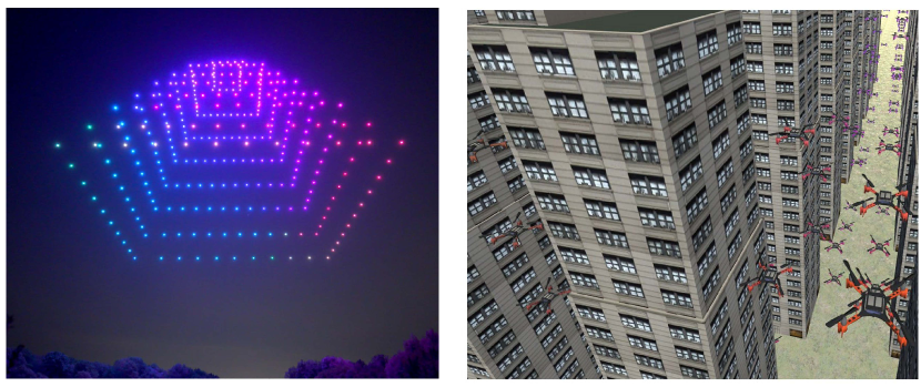
Figure 1: [left] A real-world drone light show where the UAVs form a 3D grid like pattern [29]. [right] Our simulated large UAV swarm in the Unity environment with many tall buildings as obstacles. A video of the simulations and experiments can be found at https://youtu.be/v8WMkX0qxXg

For up to $\frac{1}{3}$ of the grid vertices occupied with robots, which is very high, we perform path planning for these robots in two stages. In the first phase, we iteratively apply an algorithm based on the Rubik Table abstraction [30] to “shuffle” selected dimensions of the 3D grid. Then, the abstract shuffle operations are translated into efficient feasible robot movements. The resulting algorithm runs in low-polynomial time and achieves high levels of optimality: for uniform randomly generated instances, we show that an asymptotic makespan optimality ratio of $\frac{m_{1}+2m_{2}+2m_{3}}{m_{1}+m_{2}+m_{3}}$ is realized, which is upper bounded by $\frac{5}{3}$. Obstacles can also be supported without significant impact on solution optimality. In simulation, our algorithm easily scales to graphs with over $370,000$ vertices and $120,000$ robots. Plans computed using the two-phase process on 3D grids can be readily transformed into high-quality robot motion plans, e.g., for coordinating many aerial vehicles. We demonstrate our algorithm on large simulated quadcopter fleets in the Unity environment, and further demonstrate the execution of our algorithm on a fleet of $10$ Crazyflie 2.0 nano quadcopters.

Related Work. The literature on multi-robot coordination is vast; we focus on graph-theoretic algorithmic and complexity results here. It has been proven that solving MRPP optimally is NP-hard [31, 26], even under grid-based, obstacle-free settings [27]. Furthermore, it is also NP-hard to approximate within any factor less than $\frac{4}{3}$ for makespan minimization on graphs in general [32].

Recently, many solvers have been developed to solve MRPP with decent computational efficiency and produce high-quality solutions. MRPP solvers can be classified as being optimal or suboptimal. Reduction-based optimal solvers solve the problem through reducing the MRPP problem to other problem, e.g., SAT [33], answer set programming [34], integer linear programming (ILP) [35]. Search-based optimal MRPP solvers includes EPEA* [36], ICTS [37], CBS [38], and so on. Optimal solvers have limited scalability due to the NP-hardness of MRPP. Suboptimal solvers have also been extensively studied. Unbounded solvers like push and swap [39], push and rotate [40], windowed hierarchical cooperative A^∗ [41], all return feasible solutions very fast at the cost of solution quality. Balancing the running-time and optimality is one of the most attractive topics. Some algorithms emphasize the scalability without sacrificing too much optimality, e.g., ECBS [42], DDM [43], EECBS [44], PBS [45]. Whereas these solvers achieve fairly good scalability while maintaining $1.x$-optimality in empirical evaluations, they lack provable joint efficiency-optimality guarantees. As a result, the scalability and supported robot density of these method are on the low side as compared to our method. There are also $O(1)-$approximate or constant factor time-optimal algorithms proposed, aiming to tackle highly dense instances, e.g. [46, 27]. However, these algorithms only achieve low-polynomial time guarantee at the expense of huge constant factors, making them impractical.

This research builds on [47], which addresses the MRPP problem in 2D. In comparison to [47], the current work describes a significant extension to the 3D (as well as higher dimensional) domain with many unique applications, including, e.g., the reconfiguration of large UAV fleets, the optimal coordination of air traffic, and the adjustment of satellite constellations.

II Preliminaries

II-A Multi-Robot Path Planning on 3D Grids

We work with a graph-theoretic formulation of MRPP, which seeks collision-free paths that efficiently route many robots on graphs. Specifically, consider an undirected graph $\mathcal{G}(V,E)$ and $n$ robots with start configuration $S=\{s_{1},\dots,s_{n}\}\subseteq V$ and goal configuration $G=\{g_{1},\dots,g_{n}\}\subseteq V$. A robot $i$ has start and goal vertices $s_{i}$ and $g_{i}$, respectively. We define a path for robot $i$ as a map $P_{i}:\mathbb{N}\to V$ where $\mathbb{N}$ is the set of non-negative integers. A feasible $P_{i}$ must be a sequence of vertices that connect $s_{i}$ and $g_{i}$: 1) $P_{i}(0)=s_{i}$; 2) $\exists T_{i}\in\mathbb{N}$, s.t. $\forall t\geq T_{i},P_{i}(t)=g_{i}$; 3) $\forall t>0$, $P_{i}(t)=P_{i}(t-1)$ or $(P_{i}(t),P_{i}(t-1))\in E$.

Given the 3D focus of this work, we choose the graph $\mathcal{G}$ to be a $6$-connected $m_{1}\times m_{2}\times m_{3}$ grid with $m_{1}\geq m_{2}\geq m_{3}$, as a proper discretization of the target 3D domain. Our aim is to minimize the makespan of feasible routing plans, assuming that the transition on each edge of $G$ takes unit time. In other words, we are to compute a feasible path set $\{P_{i}\}$ that minimizes $\max_{i}\{|{P}_{i}|\}$. For most settings in this work, it is assumed that the start and goal configurations are randomly generated. Unless stated otherwise, “randomness” in this paper always refers to uniform randomness.

II-B High-Level Reconfiguration via Rubik Tables in 3D

Our method for solving the graph-based MRPP has two phases; the first high-level reconfiguration phase utilizes results on Rubik Table problems (RT3D) [30]. The Rubik Table abstraction, described below for the $k$-dimensional setting, $k\geq 2$, formalizes the task of carrying out globally coordinated token swapping operations on lattices.

Problem 1 (Rubik Table in $k$D (RTKD)).

Let $M$ be an $m_{1}\times\ldots\times m_{k}$ table, $m_{1}\geq\ldots\geq m_{k}$, containing $\prod_{i=1}^{k}m_{i}$ items, one in each table cell. In a shuffle operation, the items in a single column in the $i$-th dimension of $M$, $1\leq i\leq k$, may be permuted in an arbitrary manner. Given two arbitrary configurations $S$ and $G$ of the items on $M$, find a sequence of shuffles that take $M$ from $S$ to $G$.

We formulate Problem 1 differently from [30] (Problem 8) to make it more natural for robot coordination tasks. For convenience, let the 2D and 3D version be RT2D and RT3D, respectively. A main result from [30] (Proposition 4), applying to the 2D setting, may be stated as follows.

Proposition II.1 (Rubik Table Theorem, 2D).

An arbitrary Rubik Table problem on an $m_{1}\times m_{2}$ table can be solved using $m_{1}+2m_{2}$ column shuffles.

Denoting the corresponding algorithm for RT2D as RTA2D, we may solve RT3D using RTA2D as a subroutine, by treating RT3D as an RT2D, which is straightforward if we view a 2D slice of RTA2D as a “wide” column. For example, for the $m_{1}\times m_{2}\times m_{3}$ grid, we may treat the second and third dimensions as a single dimension. Then, each wide column, which is itself an $m_{2}\times m_{3}$ 2D problem, can be reconfigured by applying RTA2D. With some proper counting, we obtain the following 3D version of Proposition II.1.

Theorem II.1 (Rubik Table Theorem, 3D).

. An arbitrary Rubik Table problem on an $m_{1}\times m_{2}\times m_{3}$ table can be solved using $m_{1}m_{2}+m_{3}(2m_{2}+m_{1})+m_{1}m_{2}$ shuffles.

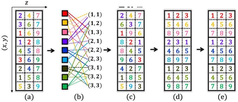
Figure 2: Illustration of applying RTA3D. (a) The initial $3\times 3\times 3$ table with a random arrangement of 27 items that are colored and labeled. A color represents the $(x,y)$ position of an item. (b) The constructed bipartite graph. The right partite set contains all the possible $(x,y)$ positions . It contains $3$ perfect matchings, determining the $3$ columns in (c). (c) Applying $z$-shuffles to (a), according to the matching results, leads to an intermediate table where each $x$-$y$ plane has one color appearing exactly once. (d) Applying wide shuffles to (c) correctly places the items according to their $(x,y)$ values (or colors). (e) Additional $z$-shuffles fully sort the labeled items.

Denote the corresponding algorithm for Theorem II.1 as RTA3D, we illustrate how it works on a $3\times 3\times 3$ table (in Fig. 2). RTA3D operates in three phases. In the first phase, a bipartite graph $B(T,R)$ is constructed based on the initial table configuration where the partite set $T$ are the colors of items representing the desired $(x,y)$ positions, and the set $R$ are the set of $(x,y)$ positions of items (Fig. 2(b)). An edge is added to $B$ between $t\in T$ and $r\in R$ for every item of color $t$ in row $r$. From $B(T,R)$, a set of $m_{1}m_{2}$ perfect matchings can be computed, as guaranteed by [48]. Each matching, containing $m_{3}$ edges, connects all of $T$ to all of $R$, dictates how a $x$-$y$ plane should look like after the first phase. For example, the first set of matching in solid lines in Fig. 2(b) says that the first $x$-$y$ plane should be ordered as the first table column shown in Fig. 2(c). After all matchings are processed, we get an intermediate table, Fig. 2(c). Notice that each row of Fig. 2(a) can be shuffled to yield the corresponding row of Fig. 2(c); this is the main novelty of the RTA3D. After the first phase of $m_{1}m_{2}$ $z$-shuffles, the intermediate table (Fig. 2(c)) that can be reconfigured by applying RTA2D with $m_{1}$ $x$-shuffles and $2m_{2}$ $y$-shuffles. This sorts each item in the correct $x$-$y$ positions (Fig. 2(d)). Another $m_{1}m_{2}$ $z$-shuffles can then sort each item to its desired $z$ position (Fig. 2(e)).

III Methods

In this section, we introduce the algorithm that integrate RTA3D algorithm to solve MRPP on 3D grids; the built-in global coordination capability of RT3D naturally applies to solving makespan-optimal MRPP. We assume the grid size is $m_{1}\times m_{2}\times m_{3}$ and there are $\frac{m_{1}m_{2}m_{3}}{3}$ robots. For density less than $\frac{1}{3}$, we add virtual robots [49, 46] till reaching $\frac{1}{3}$.

III-A RTH3D: Adapting RTA3D for MRPP in 3D

Algorithm 1 outlines the high-level process for multi-robot routing coordination in 3D. In each $x$-$y$ plane, we partition the grid $\mathcal{G}$ into $3\times 3$ cells (see, e.g.,Fig. 4). Without loss of generality, we assume that $m_{1},m_{2},m_{3}$ are integer multiples of 3 and first consider the case without any obstacles for simplicity. In the first step, to make RTA3D applicable, we convert the arbitrary start and goal configurations (assuming less than $1/3$ robot density) to intermediate configurations where in each 2D plane, each $3\times 3$ cell contains no more than $3$ robots (see Fig. 3). Such configurations are called balanced configurations [47]. In practice, configurations are likely not “far” from being balanced. The balanced configurations $S_{1},G_{1}$ and corresponding paths can be computed by applying any unlabeled multi-robot path planning method.

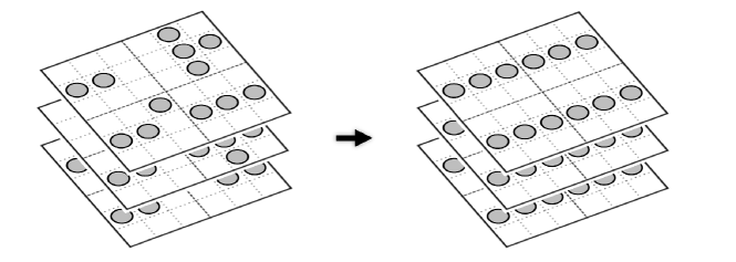
Figure 3: Applying unlabeled MRPP to convert a random configuration to a balanced centering one on $6\times 6\times 3$ grids.

After that, RTA3D can be applied to coordinate the robots moving toward their intermediate goal positions $G_{1}$. Function MatchingXY finds a feasible intermediate configuration $S_{2}$ and route the robots to $S_{2}$ by simulating shuffle operations along the $z$ axis. Function XY-Fitting apply shuffle operations along the $x$ and $y$ axes to route each robot $i$ to its desired $x$-$y$ position $(g_{1i}.x,g_{1i}.y)$. In the end, function Z-Fitting is called, routing each robot $i$ to the desired $g_{1i}$ by performing shuffle operations along the $z$ axis and concatenate the paths computed by unlabeled MRPP planner UnlabeledMRPP.

1

Input: Start and goal vertices $S=\{s_{i}\}$ and $G=\{g_{i}\}$

2 Function RTH3D($S,G$):

3       $S_{1},G_{1}\leftarrow$UnlabeledMRPP($S,G$)

4       MatchingXY()

5       XY-Fitting()

6       Z-Fitting()

7      

Algorithm 1 RTH3D

We now explain each part of RTH3D. MatchingXY uses an extended version of RTA3D to find perfect matching that allows feasible shuffle operations. Here, the “item color” of an item $i$ (robot) is the tuple $(g_{1i}.x,g_{1i}.y)$, which is the desired $x$-$y$ position it needs to go. After finding the $m_{3}$ perfect matchings, the intermediate configuration $S_{2}$ is determined. Then, shuffle operations along the $z$ direction can be applied to move the robots to $S_{2}$.

Input: Balanced start and goal vertices $S_{1}=\{s_{1i}\}$ and $G_{1}=\{g_{1i}\}$

1 Function MatchingXY($S_{1},G_{1}$):

2       $A\leftarrow[1,...,n]$

3       $\mathcal{T}\leftarrow$ the set of $(x,y)$ positions in $S_{1}$

4       for $(r,t)\in\mathcal{T}\times\mathcal{T}$ do

5             if $\exists i\in A$ where $(s_{1i}.x,s_{1i}.y)=r\wedge(g_{1i}.x,g_{1i}.y)=t$ then

6                   add edge $(r,t)$ to $B(T,R)$

7                   remove $i$ from $A$

8                  

9            

10      compute matchings $\mathcal{M}_{1},...,\mathcal{M}_{m_{3}}$ of $B(T,R)$

11       $A\leftarrow[1,...,n]$

12       foreach $\mathcal{M}_{c}$ and $(r,t)\in\mathcal{M}_{c}$ do

13             if $\exists i\in A$ where $(s_{1i}.x,s_{1i}.y)=r\wedge(g_{1i}.x,g_{1i}.y)=t$ then

14                   $s_{2i}\leftarrow(s_{1i}.x,s_{1i}.y,c)$ and remove $i$ from $A$

15                   mark robot $i$ to go to $s_{2i}$

16                  

17            

18      perform simulated $z$-shuffles in parallel

19      

Algorithm 2 MatchingXY

The robots in each $x$-$y$ plane will be reconfigured by applying $x$-shuffles and $y$-shuffles. We need to apply RTA2D for these robots in each plane, as demonstrated in Algorithm 3. In RTH2D, for each 2D plane, the “item color” for robot $i$ is its desired $x$ position $g_{1i}.x$. For each plane, we compute the $m_{2}$ perfect matchings to determine the intermediate position $g_{2}$. Then each robot $i$ moves to its $g_{2i}$ by applying $y$-shuffle operations. In Line 18, each robot is routed to its desired $x$ position by performing $x$-shuffle operations. In Line 19, each robot is routed to its desired $y$ position by performing $y$-shuffle operations.

Input: Current positions $S_{2}$ and balanced goal positions $G_{1}$

1 Function XY-Fitting():

2       for $z\leftarrow[1,...,m_{3}]$ do

3             $A\leftarrow\{i|s_{2i}.y=z\}$

4             RTH2D($A,z$)

5            

6      

7Function RTH2D($A,z$):

8      

9      $\mathcal{T}\leftarrow$ the set of $x$ positions of $S_{2}$

10       for $(r,t)\in\mathcal{T}\times\mathcal{T}$ do

11             if $\exists i\in A$ where $s_{2i}.x=r\wedge g_{1i}.x=t$ then

12                   if robot $i$ is not assigned then

13                         add edge $(r,t)$ to $B(T,R)$

14                         mark $i$ assigned

15                        

16                  

17            compute matchings $\mathcal{M}_{1},...,\mathcal{M}_{m_{2}}$ of $B(T,R)$

18            

19      $A^{\prime}\leftarrow A$

20       foreach $\mathcal{M}_{c}$ and $(r,t)\in\mathcal{M}_{c}$ do

21             if $\exists i\in A^{\prime}$ where $s_{2i}.x=c\wedge g_{1i}.x=t$ then

22                   $g_{2i}\leftarrow(s_{2i}.x,c,z)$ and remove $i$ from $A^{\prime}$

23                   mark robot $i$ to go to $g_{2i}$

24                  

25            

26      route each robot $i\in A$ to $g_{2i}$

27       route each robot $i\in A$ to $(g_{2i}.x,g_{1i}.y,z)$

28       route each robot $i\in A$ to $(g_{1i}.x,g_{1i}.y,z)$

29      

30

Algorithm 3 XY-Fitting

After all the robots reach the desired $x$-$y$ positions, another round of $z$-shuffle operations in Z-Fitting can route the robots to the balanced goal configuration computed by an unlabeled MRPP planner. In the end, we concatenate all the paths as the result.

III-B Efficient Shuffle Operation with High-Way Heuristics

In this section, we explain how to simulate the shuffle operation exactly. We use the shuffle operation in $x$-$y$ plane as an example. We partition the grid $\mathcal{G}$ into $3\times 3$ cells (see, e.g., Fig. 4). Without loss of generality, we assume that $m$ is an integer multiple of 3 and first consider the case without any obstacles for simplicity.

We use Fig. 4, where Fig. 4(a) is the initial start configuration and Fig. 4(d) is the desired goal configuration in MatchingXY, as an example to illustrate how to simulate the shuffle operations.

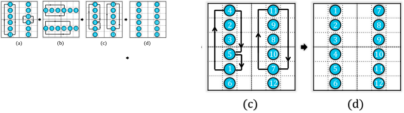
Figure 4: An example of applying RTH2D to solve an instance. (a) The initial configuration; (b) The intermediate configuration obtained from matching; (d) The desired configuration;

In MatchingXY, the initial configuration is a vertical “centered” configuration (Fig. 4 (a)). RTA3D is applied with a highway heuristic to get us from Fig. 4(b) to Fig. 4(c), transforming between vertical centered configurations and horizontal centered configurations. To do so, RTA3D is applied (e.g., to Fig. 4) to obtain two intermediate configurations (e.g., Fig. 4(b)(c)). To go between these configurations, e.g., Fig. 4(b)$\to$Fig. 4(c), we apply a heuristic by moving robots that need to be moved out of a $3\times 3$ cell to the two sides of the middle columns of Fig. 4(b), depending on their target direction. If we do this consistently, after moving robots out of the middle columns, we can move all robots to their desired goal $3\times 3$ cell without stopping nor collision. Once all robots are in the correct $3\times 3$ cells, we can convert the balanced configuration to a centered configuration in at most $3$ steps, which is necessary for carrying out the next simulated row/column shuffle. Adding things up, we can simulate a shuffle operation using no more than $m+5$ steps.

III-C Improving Solution Quality via Optimized Matching

The matching steps in RTA3D determine all the intermediate positions and therefore have great impact on solution optimality. Finding arbitrary perfect matchings is fast but can be further optimized. We replace the matching method from finding arbitrary perfect matchings to finding a min-cost matching in both of MatchingXY and RTH2D.

The matching heuristic we developed is based on linear bottleneck assignment (LBA), which runs in polynomial time. A 2D version of the heuristic is introduced in [47], to which readers are referred to for more details. Here, we illustrate how to apply LBA-matching in MatchingXY. For the matching assigned to height $z$, the edge weight of the bipartite graph is computed greedily. If a vertical column $c=(x,y)$ contains robots of “color” $t$, here $t=(g_{2}.x,g_{2}.y)$, we add an edge $(c,t)$ and its edge cost is

$$C_{ct}=\min_{(g_{2i}.x,g_{2i}.y)=t}C_{zi}(\lambda=0).$$ (1)

We choose $\lambda=0$ to optimize the first phase. Optimizing the third phase ($\lambda=1$) would give similar results. After constructing the weighted bipartite graph, an $O(m^{2.5}/\log m)$ LBA algorithm [50] is applied to get a minimum bottleneck cost matching for height $z$. Then we remove the assigned robots and compute the next minimum bottleneck cost matching for next height. After getting all the matchings $\mathcal{M}_{z}$, we can further use LBA to assign $\mathcal{M}_{z}$ to a different height $z^{\prime}$ to get a smaller makespan lower bound. The cost for assigning matching $\mathcal{M}_{z}$ to height $z^{\prime}$ is defined as

$$C_{\mathcal{M}_{z}z^{\prime}}=\max_{i\in\mathcal{M}_{z}}C_{z^{\prime}i}(\lambda=0).$$ (2)

The same approach can also be applied to RTH2D. We denote RTH3D with LBA heuristics as RTH3D-LBA.

IV Theoretical Analysis

First, we introduce two important lemmas about well-connected grids which have been proven in [46].

Lemma IV.1.

On an $m_{1}\times m_{2}\times m_{3}$ grid, any unlabeled MRPP can be solved using $O(m_{1}+m_{2}+m_{3})$ makespan.

Lemma IV.2.

On an $m_{1}\times m_{2}\times m_{3}$ grid, if the underestimated makespan of an MRPP instance is $d_{g}$ (usually computed by ignoring the inter-robot collisions), then this instance can be solved using $O(d_{g})$ makespan.

We proceed to analyze the time complexity of RTH3D on $m_{1}\times m_{2}\times m_{3}$ grids. The dominant parts of RTH3D are computing the perfect matchings and solving unlabeled MRPP. First we analyze the running time for computing the matchings. Finding $m_{3}$ “wide column” matchings runs in $O(m_{3}m_{1}^{2}m_{2}^{2})$ deterministic time or $O(m_{3}m_{1}m_{2}\log(m_{1}m_{2}))$ expected time. We apply RTH2D for simulating “wide column” shuffle, which requires $O(m_{3}m_{1}^{2}m_{2})$ deterministic time or $O(m_{1}m_{2}m_{3}\log m_{1})$ expected time. Therefore, the total time complexity for Rubik Table part is $O(m_{3}m_{1}^{2}m_{2}^{2}+m_{1}^{2}m_{2}m_{3})$. For unlabeled MRPP, we can use the max-flow based algorithm [51] to compute the makespan-optimal solutions. The max-flow portion can be solved in $O(n|E|T)=O(n^{2}(m_{1}+m_{2}+m_{3}))$ where $|E|$ is the number of edges and $T=O(m_{1}+m_{2}+m_{3})$ is the time horizon of the time expanded graph [52]. Note that any unlabeled MRPP can be applied, for example, the algorithm in [53] is distance-optimal but with convergence time guarantee.

Note that the choice of 2D plane can also be $x$-$z$ plane or $y$-$z$ plane. In addition, one can also perform two “wide column” shuffles plus one $z$ shuffle, which yields $2(2m_{1}+m_{2})+m_{3}$ number of shuffles and $O(m_{1}m_{2}m_{3}^{2}+m_{3}m_{1}m_{2}^{2})$. This requires more shuffles but shorter running time.

Next, we derive the optimality guarantee.

Proposition IV.1 (Makespan Upper Bound).

RTH3D returns solution with worst makespan $3m_{1}+4m_{2}+4m_{3}+o(m_{1})$.

Proof.

The Rubik Table portion has a makespan of $(2m_{3}+2m_{2}+m_{1})+o(m_{1})$. For the unlabeled MRPP portion, we use $m_{1}+m_{2}+m_{3}$, which is the maximum grid distance between any two nodes on the $m_{1}\times m_{2}\times m_{3}$ grid, as a conservative makespan upper bound. Therefore, the total makespan upper bound is $2(m_{1}+m_{2}+m_{3})+(2m_{3}+2m_{2}+m_{1})+o(m_{1})=3m_{1}+4m_{2}+4m_{3}+o(m_{1}).$ When $m_{1}=m_{2}=m_{3}$ for cubic grids, it turns out to be $11m_{3}+o(m_{3}).$ ∎

We note that the unlabeled MRPP upper bound is actually a very conservative estimation. In practice, for such dense instances, the unlabeled MRPP usually requires much fewer steps. Next, we analyze the makespan when start and goal configurations are uniformly randomly generated based on the well-known minimax grid matching result.

Theorem IV.1 (Multi-dimensional Minimax Grid Matching [54] ).

For $k\geq 3,$ consider $N$ points following the uniform distribution in $[0,N^{1/k}]^{k}$. Let $\mathcal{L}$ be the minimum length such that there exists a perfect matching of the $N$ points to the grid points that are regularly spaced in the $[0,N^{1/k}]^{k}$ for which the distance between every pair of matched points is at most $\mathcal{L}$. Then $\mathcal{L}=O(\log^{1/k}N)$ with high probability.

Proposition IV.2 (Asymptotic Makespan).

RTH3D returns solutions with $m_{1}+2m_{2}+2m_{3}+o(m_{1})$ asymptotic makespan for MRPP instances with $\frac{m_{1}m_{2}m_{3}}{3}$ random start and goal configurations on 3D grids, with high probability. Moreover, if $m_{1}=m_{2}=m_{3}$, RTH3D returns $5m_{3}+o(m_{3})$ makespan-optimal solutions.

Proof.

First, we point out that the theorem of minimax grid matching (Theorem IV.1) can be generalized to any rectangular cuboid as the matching distance mainly depends on the discrepancy of the start and goal distributions, which does not depend on the shape of the grid. Using the minimax grid matching result, the matching distance from a random configuration to a centering configuration, which is also the underestimated makespan of unlabeled MRPP, scales as $O(\log^{1/3}m_{1})$. Using the Lemma IV.2, it is not difficult to see that the matching obtained this way can be readily turned into an unlabeled MRPP plan without increasing the maximum per robot travel distance by much, which remains at $o(m)$. Therefore, the asymptotic makespan of RTH3D is $m_{1}+2m_{2}+2m_{3}+O(\log^{1/3}m_{1})=m_{1}+2m_{2}+2m_{3}+o(m_{1})$ with high probability. If $m_{1}=m_{2}=m_{3}$, the asymptotic makespan is $5m_{3}+o(m_{3})$, with high probability. ∎

Proposition IV.3 (Asymptotic Makespan Lower Bound).

For MRPP instances on $m_{1}\times m_{2}\times m_{3}$ grids with $\Theta(m_{1}m_{2}m_{3})$ random start and goal configurations on 3D grids, the makespan lower bound is asymptotically approaching $m_{1}+m_{2}+m_{3}$, with high probability.

Proof.

We examine two opposite corners of the $m_{1}\times m_{2}\times m_{3}$ grid. At each corner, we examine an $\alpha m_{1}\times\alpha m_{2}\times\alpha m_{3}$ sub-grid for some constant $\alpha\ll 1$. The Manhattan distance between a point in the first sub-grid and another point in the second sub-grid is larger than $(1-6\alpha)(m_{1}+m_{2}+m_{3})$. As $m\to\infty$, with $\Theta(m^{3})$ robots, a start-goal pair falling into these two sub-grids can be treated as an event following binomial distribution $B(k,\alpha^{6})$ when $m\rightarrow\infty$. The probability of having at least one success trial among $n$ trials is $p=1-(1-\alpha^{6})^{n}$, which goes to one when $m\rightarrow\infty$.

Because $(1-x)^{y}<e^{-xy}$ for $0<x<1$ and $y>0$, $p>1-e^{-\alpha^{6}n}$. Therefore, for arbitrarily small $\alpha$, we may choose $m_{1}$ such that $p$ is arbitrarily close to $1$. The probability of a start-goal pair falling into these two sub-grids is asymptotically approaching one , meaning that the makespan goes to $(1-6\alpha)(m_{1}+m_{2}+m_{3})$. ∎

Corollary IV.1 (Asymptotic Makespan Optimality Ratio).

RTH3D yields asymptotic $1+\frac{m_{2}+m_{3}}{m_{1}+m_{2}+m_{3}}$ makespan optimality ratio for MRPP instances with $\Theta(m_{1}m_{2}m_{3})\leq\frac{m_{1}m_{2}m_{3}}{3}$ random start and goal configurations on 3D grids, with high probability.

Proof.

If $n<\frac{m_{1}m_{2}m_{3}}{3}$, we add virtual robots with randomly generated start and use the same for the goal, until we reach $n=\frac{m_{1}m_{2}m_{3}}{3}$ robots, which then allows us to invoke Proposition IV.2. In viewing Proposition IV.2 and Proposition IV.3, solution computed by RTH3D guarantees a makespan optimality ratio of $\frac{m_{1}+2m_{2}+2m_{3}}{m_{1}+m_{2}+m_{3}}=1+\frac{m_{2}+m_{3}}{m_{1}+m_{2}+m_{3}}$ as $m_{3}\to\infty$. Moreover, if $m_{1}=m_{2}=m_{3}$, RTH3D returns $\frac{5}{3}$ makespan-optimal solution. ∎

Corollary IV.2 (Asymptotic Optimality, Fixed Height).

For an MRPP on an $m_{1}\times m_{2}\times K$ grid, $m_{1}>m_{2}\gg K$, and $\frac{1}{3}$ robot density, the RTH3D algorithm yields $1+\frac{m_{1}}{m_{1}+m_{2}}$ optimality ratio, with high probability. If $m_{1}=m_{2}$, the asymptotic makespan optimality ratio is $1.5$.

Theorem IV.2.

Consider an $k$-dimensional cubic grid with grid size $m$. If robot density is less than $1/3$ and start and goal configurations are uniformly distributed, generalizations to RTA3D can solve the instance with asymptotic makespan optimality being $\frac{2^{k-1}+1}{k}$.

Proof.

By theorem IV.1, the unlabeled MRPP takes $o(m)$ makespan (note for $k=1,2$, the minimax grid matching distance is still $o(m)$ [55]). Extending proposition IV.3 to $k$-dimensional grid, the asymptotic lower bound is $mk$. We now prove that the asymptotic makespan $f(k)$ is $(2^{k-1}+1)m+o(m)$ by induction. The Rubik Table algorithm solves a $d$-dimensional problem by using two 1-dimensional shuffles and one $(k-1)$-dimensional “wide column” shuffle. Therefore, we have $f(k)=2m+f(k-1)$. It’s trivial to see $f(1)=m+o(m),f(2)=3m+o(m)$, which yields that $f(k)=2^{k-1}m+m+o(m)$ and makespan optimality ratio being $\frac{2^{k-1}+1}{k}$. ∎

V Simulations And Experiments

In this section, we evaluate the performance of our polynomial time, asymptotic optimal algorithms and compare them with fast and near-optimal solvers, ECBS ($w$=1.5) [42] and ILP with 16-split heuristic [35, 56]. For the unlabeled MRPP planner, we use the algorithm [53]. Though it minimizes total distance, we find it is much faster than max-flow method [51] and the makespan optimality is very close to the optimal one on well-connected grids. All the algorithms are implemented in C++. We mention that, though not presented here, we also evaluated push-and-swap [39], which yields good computation time but substantially worse optimality (with ratio $>25$) on the large and dense settings we attempt. We also examined prioritized methods, e.g., [45, 41], which faced significant difficulties in resolving deadlocks. All experiments are performed on an Intel^® Core^TM i7-9700 CPU at 3.0GHz. Each data point is an average over 20 runs on randomly generated instances, unless otherwise stated. A running time limit of $300$ seconds is imposed over all instances. The optimality ratio is estimated as compared to conservatively estimated lower bound.

In addition to numerical evaluations, we further demonstrate using RTA3D-LBA to coordinate many UAVs in the Unity [57] environment as well as to plan trajectories for $10$ Crazyflie 2.0 nano quadcopter in 3D. We will make our source code available upon the publication of this work.

V-A Evaluations on 3D Grids

In the first evaluation, we fix the aspect ratio $m_{1}:m_{2}:m_{3}=4:2:1$ and $\frac{1}{3}$ robot density, and examine the performance RTA3D methods on obstacle-free grids with varying size. Start and goal configurations are randomly generated; the results are shown in Fig. 5. ILP with 16-split heuristic and ECBS computes solution with better optimality ratio but have poor scalability. In contrast, RTH3D and RTH3D-LBA readily scale to grids with over $370,000$ vertices and $120,000$ robots. Both of the optimality ratio of RTH3D and RTH3D-LBA decreases as the grid size increases, asymptotically approaching $\sim 1.7$ for RTH3D and $\sim 1.5$ for RTH3D-LBA.

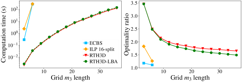
Figure 5: Computation time and optimality ratio on grids with varying grid size and $m_{1}:m_{2}:m_{3}=4:2:1$.

In a second evaluation, we fix $m_{1}:m_{2}=1:1,m_{3}=6$ and robot density at $\frac{1}{3}$, and vary $m_{1}$. As shown in Fig. 6, RTH3D and RTH3D-LBA show exceptional scalability and the asymptotic 1.5 makespan optimality ratio, as predicted by Corollary IV.2.

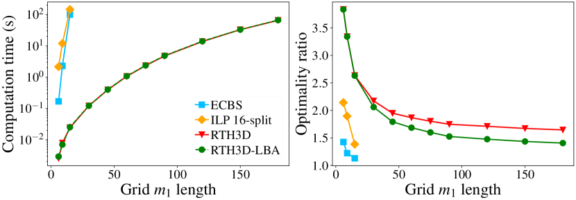
Figure 6: Computation time and optimality ratio on grids with $m_{1}:m_{2}=1$ and $m_{3}=6$.

RTH3D and RTH3D-LBA support scattered obstacles where obstacles are small and regularly distributed. As a demonstration of this capability, we simulate setting with an environment containing many tall buildings, a snapshot of which is shown Fig. 1. These “tall building” obstacles are located at positions $(3i+1,3j+1)$, which corresponds to an obstacle density of over $10\%$. UAV swarms have to avoid colliding with the tall buildings and are not allowed to fly higher than those buildings. We fix the aspect ratio at $m_{1}:m_{2}:m_{3}=4:2:1$ and robot density at $\frac{2}{9}$. The evaluation result is shown in Fig. 7.

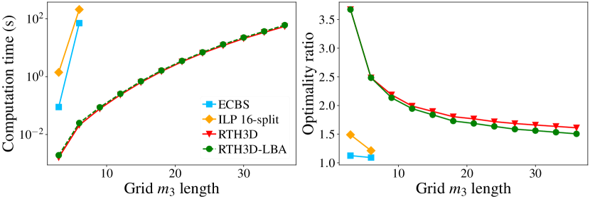
Figure 7: Computation time and optimality ratio on 3D environments with obstacles. $m_{1}:m_{2}:m_{3}=4:2:1$.

V-B Impact of Robot Density

Next, we vary robot density, fixing the environment as a $120\times 60\times 6$ grid. For robot density lower than $\frac{1}{3}$, we add virtual robots with random start and goal configurations for perfect matching computation. When applying the shuffle operations and evaluating optimality ratios, virtual robots are removed. Therefore, the optimality ratio is not overestimated. The result is plotted in Fig. 8, showing that robot density has little impact on the running time. On the other hand, as robot density increases, the lower bound and the makespan required by unlabeled MRPP are closer to theoretical limits. Thus, the makespan optimality ratio is actually better.

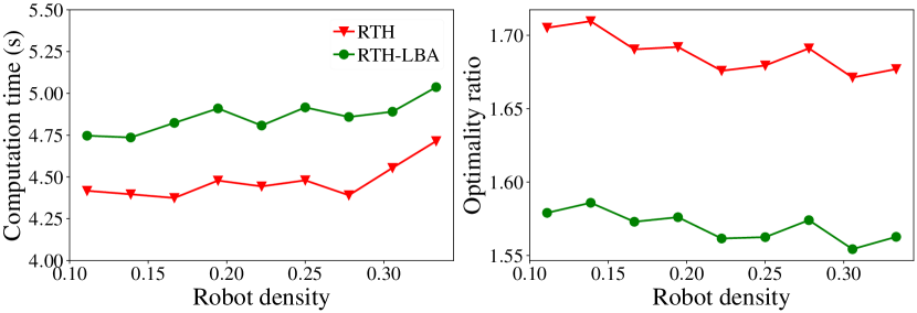
Figure 8: Computation time and optimality ratio on a $120\times 60\times 6$ grid with varying robot density.

V-C Special Patterns

In addition to random instances, we also tested instances with start and goal configurations forming special patterns, e.g., 3D “ring” and “block” structures (Fig. 9). For both settings, $m_{1}=m_{2}=m_{3}$. In the first setting, “rings”, robots form concentric square rings in each $x$-$y$ plane. Each robot and its goal are centrosymmetric. In the “block” setting, the grid is divided to $27$ smaller cubic blocks. The robots in one block need to move to another random chosen block. Fig. 9(c) shows the optimality ratio results of both settings on grids with varying size. Notice that the optimality ratio for the ring approaches $1$ for large environments.

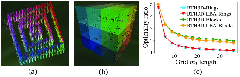
Figure 9: Special patterns and the associated optimality ratios.

V-D Crazyswarm Experiment

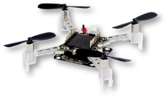
Figure 10: Crazyflie 2.0 nano quadcopter.

Paths planned by RTA3D can also be readily transferred to real UAVs. To demonstrate this, $10$ Crazyflie 2.0 nano quadcopters are choreographed to form the “A-R-C-R-U” pattern, letter by letter, on $6\times 6\times 6$ grids (Fig. 11).

The discrete paths are computed by RTH3D. Due to relatively low robot density, shuffle operations are further optimized to be more efficient. Continuous trajectories are then computed based on RTH3D plans by applying the method described in [25].

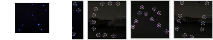
Figure 11: A Crazyswarm [58] with 10 Crazyflies following paths computed by RTA3D on $6\times 6\times 6$ grids, transitioning between letters ARC-RU. The figure shows five snapshots during the process. We note that some letters are skewed in the pictures which is due to non-optimal camera angles when the videos were taken.

VI Conclusion

In this study, we proposed to apply Rubik Table results [30] to solve MRPP. Combining RTA3D, efficient shuffling, and matching heuristics, we obtain a novel polynomial time algorithm, RTH3D-LBA, that is provably $1.x$ makespan-optimal with up to $\frac{1}{3}$ robot density. In practice, our methods can solve problems on graphs with over $300,000$ vertices and $100,000$ robots to $1.5$ makespan-optimal. Paths planned by RTH3D-LBA readily translate to high quality trajectories for coordinating large number of UAVs and are demonstrated on a real UAV fleet.

In future work, we plan to expand in several directions, enhancing both the theoretical guarantees and the methods’ practical applicability. In particular, we are interested in planning better paths that carefully balance between the nominal solution path optimality at the grid level and the actual path optimality during execution, which requires the consideration of the dynamics of the aerial vehicles that are involved. We will also address domain-specific issues for UAV coordination, e.g., down-wash, possibly employing learning-based methods [59].

References

- [1] M. A. Erdmann and T. Lozano-Pérez, “On multiple moving objects,” in Proceedings IEEE International Conference on Robotics & Automation, 1986, pp. 1419–1424.
- [2] S. M. LaValle and S. A. Hutchinson, “Optimal motion planning for multiple robots having independent goals,” IEEE Transactions on Robotics & Automation, vol. 14, no. 6, pp. 912–925, Dec. 1998.
- [3] Y. Guo and L. E. Parker, “A distributed and optimal motion planning approach for multiple mobile robots,” in Proceedings IEEE International Conference on Robotics & Automation, 2002, pp. 2612–2619.
- [4] J. van den Berg, M. C. Lin, and D. Manocha, “Reciprocal velocity obstacles for real-time multi-agent navigation,” in Proceedings IEEE International Conference on Robotics & Automation, 2008, pp. 1928–1935.
- [5] T. Standley and R. Korf, “Complete algorithms for cooperative pathfinding problems,” in Proceedings International Joint Conference on Artificial Intelligence, 2011, pp. 668–673.
- [6] K. Solovey and D. Halperin, “-color multi-robot motion planning,” in Proceedings Workshop on Algorithmic Foundations of Robotics, 2012.
- [7] M. Turpin, K. Mohta, N. Michael, and V. Kumar, “CAPT: Concurrent assignment and planning of trajectories for multiple robots,” International Journal of Robotics Research, vol. 33, no. 1, pp. 98–112, 2014.
- [8] K. Solovey, J. Yu, O. Zamir, and D. Halperin, “Motion planning for unlabeled discs with optimality guarantees,” in Robotics: Science and Systems, 2015.
- [9] G. Wagner, “Subdimensional expansion: A framework for computationally tractable multirobot path planning,” 2015.
- [10] L. Cohen, T. Uras, T. Kumar, H. Xu, N. Ayanian, and S. Koenig, “Improved bounded-suboptimal multi-agent path finding solvers,” in International Joint Conference on Artificial Intelligence, 2016.
- [11] B. Araki, J. Strang, S. Pohorecky, C. Qiu, T. Naegeli, and D. Rus, “Multi-robot path planning for a swarm of robots that can both fly and drive,” in IEEE Int. Conf. on Robotics and Automation (ICRA), 2017.
- [12] S. Tang and V. Kumar, “A complete algorithm for generating safe trajectories for multi-robot teams,” in Robotics Research. Springer, 2018, pp. 599–616.
- [13] H. Wang and M. Rubenstein, “Walk, stop, count, and swap: decentralized multi-agent path finding with theoretical guarantees,” IEEE Robotics and Automation Letters, vol. 5, no. 2, pp. 1119–1126, 2020.
- [14] D. Halperin, J.-C. Latombe, and R. Wilson, “A general framework for assembly planning: The motion space approach,” Algorithmica, vol. 26, no. 3-4, pp. 577–601, 2000.
- [15] S. Rodriguez and N. M. Amato, “Behavior-based evacuation planning,” in Proceedings IEEE International Conference on Robotics & Automation, 2010, pp. 350–355.
- [16] S. Poduri and G. S. Sukhatme, “Constrained coverage for mobile sensor networks,” in Proceedings IEEE International Conference on Robotics & Automation, 2004.
- [17] B. Smith, M. Egerstedt, and A. Howard, “Automatic generation of persistent formations for multi-agent networks under range constraints,” ACM/Springer Mobile Networks and Applications Journal, vol. 14, no. 3, pp. 322–335, Jun. 2009.
- [18] D. Fox, W. Burgard, H. Kruppa, and S. Thrun, “A probabilistic approach to collaborative multi-robot localization,” Autonomous Robots, vol. 8, no. 3, pp. 325–344, Jun. 2000.
- [19] E. J. Griffith and S. Akella, “Coordinating multiple droplets in planar array digital microfluidic systems,” International Journal of Robotics Research, vol. 24, no. 11, pp. 933–949, 2005.
- [20] D. Rus, B. Donald, and J. Jennings, “Moving furniture with teams of autonomous robots,” in Proceedings IEEE/RSJ International Conference on Intelligent Robots & Systems, 1995, pp. 235–242.
- [21] J. S. Jennings, G. Whelan, and W. F. Evans, “Cooperative search and rescue with a team of mobile robots,” in Proceedings IEEE International Conference on Robotics & Automation, 1997.
- [22] R. A. Knepper and D. Rus, “Pedestrian-inspired sampling-based multi-robot collision avoidance,” in 2012 IEEE RO-MAN: The 21st IEEE International Symposium on Robot and Human Interactive Communication. IEEE, 2012, pp. 94–100.
- [23] P. R. Wurman, R. D’Andrea, and M. Mountz, “Coordinating hundreds of cooperative, autonomous vehicles in warehouses,” AI magazine, vol. 29, no. 1, pp. 9–9, 2008.
- [24] R. Mason, “Developing a profitable online grocery logistics business: Exploring innovations in ordering, fulfilment, and distribution at ocado,” in Contemporary Operations and Logistics. Springer, 2019, pp. 365–383.
- [25] W. Hönig, J. A. Preiss, T. S. Kumar, G. S. Sukhatme, and N. Ayanian, “Trajectory planning for quadrotor swarms,” IEEE Transactions on Robotics, vol. 34, no. 4, pp. 856–869, 2018.
- [26] J. Yu and S. M. LaValle, “Structure and intractability of optimal multi-robot path planning on graphs,” in Twenty-Seventh AAAI Conference on Artificial Intelligence, 2013.
- [27] E. D. Demaine, S. P. Fekete, P. Keldenich, H. Meijer, and C. Scheffer, “Coordinated motion planning: Reconfiguring a swarm of labeled robots with bounded stretch,” SIAM Journal on Computing, vol. 48, no. 6, pp. 1727–1762, 2019.
- [28] J. E. Hopcroft, J. T. Schwartz, and M. Sharir, “On the complexity of motion planning for multiple independent objects; pspace-hardness of the” warehouseman’s problem”,” The International Journal of Robotics Research, vol. 3, no. 4, pp. 76–88, 1984.
- [29] “Duke energy drone light show at the st. pete pier,” https://stpetepier.org/anniversary/, accessed: 2022-02-16.
- [30] M. Szegedy and J. Yu, “On rearrangement of items stored in stacks,” in The 14th International Workshop on the Algorithmic Foundations of Robotics, 2020.
- [31] P. Surynek, “An optimization variant of multi-robot path planning is intractable,” in Proceedings of the AAAI Conference on Artificial Intelligence, vol. 24, no. 1, 2010.
- [32] H. Ma, C. Tovey, G. Sharon, T. Kumar, and S. Koenig, “Multi-agent path finding with payload transfers and the package-exchange robot-routing problem,” in Proceedings of the AAAI Conference on Artificial Intelligence, vol. 30, no. 1, 2016.
- [33] P. Surynek, “Towards optimal cooperative path planning in hard setups through satisfiability solving,” in Pacific Rim International Conference on Artificial Intelligence. Springer, 2012, pp. 564–576.
- [34] E. Erdem, D. G. Kisa, U. Oztok, and P. Schüller, “A general formal framework for pathfinding problems with multiple agents,” in Twenty-Seventh AAAI Conference on Artificial Intelligence, 2013.
- [35] J. Yu and S. M. LaValle, “Optimal multirobot path planning on graphs: Complete algorithms and effective heuristics,” IEEE Transactions on Robotics, vol. 32, no. 5, pp. 1163–1177, 2016.
- [36] M. Goldenberg, A. Felner, R. Stern, G. Sharon, N. Sturtevant, R. C. Holte, and J. Schaeffer, “Enhanced partial expansion a,” Journal of Artificial Intelligence Research, vol. 50, pp. 141–187, 2014.
- [37] G. Sharon, R. Stern, M. Goldenberg, and A. Felner, “The increasing cost tree search for optimal multi-agent pathfinding,” Artificial Intelligence, vol. 195, pp. 470–495, 2013.
- [38] G. Sharon, R. Stern, A. Felner, and N. R. Sturtevant, “Conflict-based search for optimal multi-agent pathfinding,” Artificial Intelligence, vol. 219, pp. 40–66, 2015.
- [39] R. J. Luna and K. E. Bekris, “Push and swap: Fast cooperative path-finding with completeness guarantees,” in Twenty-Second International Joint Conference on Artificial Intelligence, 2011.
- [40] B. De Wilde, A. W. Ter Mors, and C. Witteveen, “Push and rotate: a complete multi-agent pathfinding algorithm,” Journal of Artificial Intelligence Research, vol. 51, pp. 443–492, 2014.
- [41] D. Silver, “Cooperative pathfinding.” Aiide, vol. 1, pp. 117–122, 2005.
- [42] M. Barer, G. Sharon, R. Stern, and A. Felner, “Suboptimal variants of the conflict-based search algorithm for the multi-agent pathfinding problem,” in Seventh Annual Symposium on Combinatorial Search, 2014.
- [43] S. D. Han and J. Yu, “Ddm: Fast near-optimal multi-robot path planning using diversified-path and optimal sub-problem solution database heuristics,” IEEE Robotics and Automation Letters, vol. 5, no. 2, pp. 1350–1357, 2020.
- [44] J. Li, W. Ruml, and S. Koenig, “Eecbs: A bounded-suboptimal search for multi-agent path finding,” in Proceedings of the AAAI Conference on Artificial Intelligence (AAAI), 2021.
- [45] H. Ma, D. Harabor, P. J. Stuckey, J. Li, and S. Koenig, “Searching with consistent prioritization for multi-agent path finding,” in Proceedings of the AAAI Conference on Artificial Intelligence, vol. 33, no. 01, 2019, pp. 7643–7650.
- [46] J. Yu, “Constant factor time optimal multi-robot routing on high-dimensional grids,” 2018 Robotics: Science and Systems, 2018.
- [47] T. Guo and J. Yu, “Sub-1.5 time-optimal multi-robot path planning on grids in polynomial time,” arXiv preprint arXiv:2201.08976, 2022.
- [48] P. Hall, “On representatives of subsets,” in Classic Papers in Combinatorics. Springer, 2009, pp. 58–62.
- [49] S. D. Han, E. J. Rodriguez, and J. Yu, “Sear: A polynomial-time multi-robot path planning algorithm with expected constant-factor optimality guarantee,” in 2018 IEEE/RSJ International Conference on Intelligent Robots and Systems (IROS). IEEE, 2018, pp. 1–9.
- [50] R. Burkard, M. Dell’Amico, and S. Martello, Assignment problems: revised reprint. SIAM, 2012.
- [51] J. Yu and S. M. LaValle, “Multi-agent path planning and network flow,” in Algorithmic foundations of robotics X. Springer, 2013, pp. 157–173.
- [52] L. R. Ford and D. R. Fulkerson, “Maximal flow through a network,” Canadian journal of Mathematics, vol. 8, pp. 399–404, 1956.
- [53] J. Yu and M. LaValle, “Distance optimal formation control on graphs with a tight convergence time guarantee,” in 2012 IEEE 51st IEEE Conference on Decision and Control (CDC). IEEE, 2012, pp. 4023–4028.
- [54] P. W. Shor and J. E. Yukich, “Minimax grid matching and empirical measures,” The Annals of Probability, vol. 19, no. 3, pp. 1338–1348, 1991.
- [55] T. Leighton and P. Shor, “Tight bounds for minimax grid matching with applications to the average case analysis of algorithms,” Combinatorica, vol. 9, no. 2, pp. 161–187, 1989.
- [56] T. Guo, S. D. Han, and J. Yu, “Spatial and temporal splitting heuristics for multi-robot motion planning,” in IEEE International Conference on Robotics and Automation, 2021.
- [57] A. Juliani, V.-P. Berges, E. Teng, A. Cohen, J. Harper, C. Elion, C. Goy, Y. Gao, H. Henry, M. Mattar et al., “Unity: A general platform for intelligent agents,” arXiv preprint arXiv:1809.02627, 2018.
- [58] J. A. Preiss, W. Hönig, G. S. Sukhatme, and N. Ayanian, “Crazyswarm: A large nano-quadcopter swarm,” in IEEE Int. Conf. on Robotics and Automation (ICRA), 2017.
- [59] G. Shi, W. Hönig, Y. Yue, and S.-J. Chung, “Neural-swarm: Decentralized close-proximity multirotor control using learned interactions,” in 2020 IEEE International Conference on Robotics and Automation (ICRA). IEEE, 2020, pp. 3241–3247.