Muon decay and neutrino mass

Abstract

The observed neutrino oscillations lead to the conclusion that the neutrinos have a non zero mass, whereas the standard calculations of the weak leptonic decays assume they are massless. However, the experimental uncertainties in the quantities observed in such decays are able to absorb the effects of the non zero neutrino masses, provided that they are not too large, as it seems to be according to the presently established upper limits. This fact is shown in detail for the $\mu$ decay, but it can be established also for the leptonic decays of the $\tau$ meson.

1 Introduction

The neutrino oscillation is a well established phenomenon (for a review see [1]), which implies that neutrinos are massive, whereas in the Standard Model they are massless. Presently there is no direct measure of the neutrino masses and the only information is given by upper limits obtained from the beta decay [2], the $\pi^{+}decay$ [3] and the $\tau$ decay [4], for the $e$-, $\mu$- and $\tau$-types, respectively.

The problem arises of understanding if the standard description of leptonic weak processes has to be modified in order to take into account the non zero values of the neutrino masses.

In this paper it is shown that, at least for the leptonic muon decay, the V-A theoretical calculations with massive neutrinos are perfectly compatible with the observed data. This happens provided that the neutrino masses are not too high, namely within the present upper limits. In fact, if this is the case, the effects coming from the massive neutrinos are smaller than the experimental errors of the various observed quantities, such as the $\mu$ lifetime, the electron helicity and the energy and angle distributions of the outgoing electron.

As for the the $\mu$ lifetime, its high precision is such that one can obtain a limit for the $\nu$ mass (muon based) [5] more stringent than the one reported in ref. [1].

As a byproduct of the present calculations, one can verify that a similar compatibility between experimental data and the presence of a non zero value of the neutrinos masses is valid also for the leptonic decays of the $\tau$ meson.

2 The decay rate

Let us for simplicity concentrate on the decay of the negative muon, that is on the process

$$\mu^{-}\rightarrow e^{-}+\bar{\nu}_{e}+\nu_{\mu}$$ (1)

Of course, by applying the charge conjugation, the results obtained in what follows are valid also for the decay

$$\mu^{+}\rightarrow e^{+}+\nu_{e}+\bar{\nu}_{\mu}$$ (2)

The transition amplitude as reported in standard books (see for instance ref. [6]) is

$$M=\frac{G}{\sqrt{2}}[\bar{u}_{e}(p,s)\gamma^{\alpha}(1-\gamma_{5})\nu_{e}(q_{1},s_{1})][\bar{\nu}_{\mu}(q_{2},s_{2})\gamma^{\beta}(1-\gamma_{5})u_{\mu}(k,t)]$$ (3)

where $G$ is the Fermi constant, ${u}_{e}(u_{\mu})$ is the electron (muon) spinor with energy-momentum and spin p,s (k,t), while $q_{1}$ and $q_{2}$ are the tetramomenta of the two neutrinos and $s_{1},s_{2}$ are their spin components.

The decay rate is

$$d\Gamma=\frac{1}{(2\pi)^{5}}\frac{1}{2k_{0}}\delta(k-p-q_{1}-q_{2})|M|^{2}\frac{d^{3}p}{2p_{0}}\frac{d^{3}q_{1}}{2q_{10}}\frac{d^{3}q_{2}}{2q_{20}}$$ (4)

the transition strength is given by

$$|M|^{2}=\frac{G^{2}}{2}M_{\alpha\beta}E^{\alpha\beta}$$ (5)

having separated out the electron and muon factors

$$\begin{array}[]{ccc}M_{\alpha\beta}&=&[\bar{\nu}_{\mu}(q_{2},s_{2})\gamma_{\alpha}(1-\gamma_{5})u_{\mu}(k,t)][\bar{u}_{\mu}(k,t)\gamma_{\beta}(1-\gamma_{5})\nu_{\mu}(q_{2},s_{2})]\\ &&\\ E^{\alpha\beta}&=&[\bar{\nu}_{e}(q,s_{1})\gamma^{\beta}(1-\gamma_{5})u_{e}(p,s)][\bar{u}_{e}(p,s)\gamma^{\alpha}(1-\gamma_{5})\nu_{e}(q_{1},s_{1})]\end{array}$$ (9)

With the definitions

$$[kq_{2}]_{\alpha\beta}=[k_{\alpha}q_{2\beta}+k_{\beta}q_{2\alpha}-g_{\alpha\beta}(kq_{2})]$$ (10)

$$(kq_{2})_{\alpha\beta}=\epsilon_{\beta\gamma\alpha\delta}k^{\gamma}q_{2}^{\delta}$$ (11)

calculating the traces one gets

$$M_{\alpha\beta}=2[\tilde{k}\tilde{q}_{2}]_{\alpha\beta}-2i(\tilde{k}\tilde{q}_{2})_{\alpha\beta}$$ (12)

where

$$\tilde{k}=k-m_{\mu}t~{}~{}~{}~{}~{}~{}\tilde{q}_{2}=q_{2}-m_{2}s_{2}$$ (13)

$E^{\alpha\beta}$ is obtained from $M_{\alpha\beta}$ with the substitution

$$\alpha\rightarrow\beta~{}~{}~{}~{}2\rightarrow 1~{}~{}~{}~{}k\rightarrow p~{}~{}~{}~{}t\rightarrow s~{}~{}~{}~{}m_{\mu}\rightarrow m_{e}$$ (14)

$$E^{\alpha\beta}=2[\tilde{p}\tilde{q}_{1}]^{\alpha\beta}-2i(\tilde{p}\tilde{q}_{1})^{\alpha\beta}$$ (15)

where

$$\tilde{p}=p-m_{e}s~{}~{}~{}~{}~{}~{}\tilde{q}_{1}=q_{1}-m_{1}s_{1}$$ (16)

and the antisymmetry of $(\tilde{p}\tilde{q}_{1})^{\alpha\beta}$ has been taken into account.

The spins of the two neutrinos are not observed and then one has to sum over $s_{1}$ and $s_{2}$. These sums can be performed separately on $M_{\alpha\beta}$ and $E^{\alpha\beta}$. The result is that the terms linear in $s_{1}$ or $s_{2}$ disappear and the rest acquires a factor two. Performing the contractions we have

$$\Sigma_{s_{1}s_{2}}|M|^{2}=32G^{2}(\tilde{k}q_{1})(\tilde{p}q_{2})$$ (17)

Neither the momenta of the two neutrinos are observed and then one has to integrate over $d^{3}q_{1}d^{3}q_{2}$ calculating integrals of the type

$$I_{\alpha\beta}=\int\frac{d^{3}q_{1}}{2q_{10}}\frac{d^{3}q_{2}}{2q_{20}}\delta(q-q_{1}-q_{2})q_{1\alpha}q_{2\beta}$$ (18)

having defined $q=k-p$. Using standard techniques, the result is

$$I_{\alpha\beta}=\frac{\pi}{6}\alpha(q^{2})g_{\alpha\beta}+\frac{\pi}{3}\beta(q^{2})q_{\alpha}q_{\beta}$$ (19)

The expressions for $\alpha(q^{2})$ and $\beta(q^{2})$ differ substantially from the ones valid in the case of massless neutrinos. In fact we have

$$\alpha(q^{2})=q^{2}-2-2\Sigma+\frac{\Delta^{2}}{q^{2}},~{}~{}~{}~{}~{}\beta(q^{2})=1+\frac{\Sigma}{q^{2}}-\frac{2\Delta^{2}}{q^{4}}$$ (20)

where

$$\Sigma=m_{1}^{2}+m_{2}^{2},~{}~{}~{}~{}~{}~{}~{}\Delta=m_{2}^{2}-m_{1}^{2}$$ (21)

The decay rate $d\Gamma_{\nu}$, summed and integrated over all neutrino variables, is

$$d\Gamma_{\nu}=\frac{1}{(2\pi)^{4}}\frac{G^{2}}{6}\frac{1}{k_{0}p_{0}}[\alpha(q^{2})(\tilde{k}\tilde{p})+2\beta(q^{2})(q\tilde{k})(q\tilde{p})]d^{3}p$$ (22)

From now on we shall perform the calculations in the muon rest frame, where

$$k=(m_{\mu},0),~{}~{}~{}~{}t=(0,\vec{t}),~{}~{}~{}~{}p=(E,\vec{p})~{}~{}~{}~{}s=(\frac{\vec{p}\cdot\vec{n}}{m_{e}},\vec{n}+\frac{(\vec{p}\cdot\vec{n})\vec{p}}{m_{e}(E+m_{e})})$$ (23)

where $m_{e}$ ($m_{\mu}$) is the electron (muon) mass and $\vec{n}$ ($\vec{t}$) the corresponding spin vector in the muon rest frame. In particular we obtain

$$q^{2}=2m_{\mu}(W-E)$$ (24)

having introduced the standard definitions

$$W=\frac{m_{\mu}^{2}+m_{e}^{2}}{2m_{\mu}}=\frac{m_{\mu}}{2}(1+x^{2}),~{}~{}~{}~{}~{}~{}x=\frac{m_{e}^{2}}{m_{\mu}^{2}}$$ (25)

The maximum energy of the electron is

$$E_{M}=W-\frac{(m_{1}+m_{2})^{2}}{2m_{\mu}}$$ (26)

Defining the quantity

$$S=\frac{16}{Em_{\mu}^{6}}[\alpha(q^{2})(\tilde{k}\tilde{p})+2\beta(q^{2})(q\tilde{k})(q\tilde{p})]$$ (27)

the decay strength can now be written as

$$d\Gamma_{\nu}=\frac{1}{(2\pi)^{4}}m_{\mu}^{5}\frac{G^{2}}{96}Sd^{3}p$$ (28)

and $S$ can be expanded in terms of the various polarization quantities as follows

$$S=S_{0}+\vec{p}\cdot\vec{t}S_{t}+\vec{p}\cdot\vec{n}S_{n}+\vec{n}\cdot\vec{t}S_{nt}+(\vec{p}\cdot\vec{n})(\vec{p}\cdot\vec{t})S_{pnt}$$ (29)

The analytical expressions of the quantities defined in the expansion shown in Eq. (29) are given below:

$$S_{0}=\frac{32}{m_{\mu}^{4}}[3W-2E-\frac{m_{e}^{2}}{E}+\frac{\Sigma}{2m_{\mu}}\frac{E-\frac{m_{e}^{2}}{E}}{W-E}+\frac{\Delta^{2}}{4m_{\mu}^{2}}\frac{E-3W+2\frac{m_{e}^{2}}{E}}{(W-E)^{2}}]~{}~{}~{}~{}~{}~{}~{}~{}~{}~{}$$ (30)

$$S_{t}=\frac{32}{Em_{\mu}^{4}}[3W-2E-m_{\mu}+\frac{\Sigma}{2m_{\mu}}\frac{E-m_{\mu}}{W-E}+\frac{\Delta^{2}}{4m_{\mu}^{2}}\frac{E-3W+2m_{\mu}}{(W-E)^{2}}]~{}~{}~{}~{}~{}~{}~{}~{}$$ (31)

$$S_{n}=-\frac{32}{Em_{\mu}^{4}}[W-2E+m_{\mu}+\frac{\Sigma}{2m_{\mu}}\frac{E-2W+m_{\mu}}{W-E}+\frac{\Delta^{2}}{4m_{\mu}^{2}}\frac{W+E-2m_{\mu}}{(W-E)^{2}}]$$ (32)

$$S_{nt}=-\frac{32}{Em_{\mu}^{4}}m_{e}[W-E-\frac{\Sigma}{m_{\mu}}+\frac{\Delta^{2}}{4m_{\mu}^{2}}\frac{1}{W-E}]~{}~{}~{}~{}~{}~{}~{}~{}~{}~{}~{}~{}~{}~{}~{}~{}~{}~{}~{}~{}~{}~{}~{}~{}~{}~{}~{}~{}~{}~{}~{}~{}~{}~{}$$ (33)

$$S_{pnt}=\frac{32}{E(E+m_{e})m_{\mu}^{4}}[2E-W+m_{e}+\frac{\Sigma}{2m_{\mu}}\frac{2W-E+m_{e}}{(W-E)}-\frac{\Delta^{2}}{4m_{\mu}^{2}}\frac{W+E+2m_{e}}{(W-E)^{2}}]$$ (34)

The terms in $\Sigma$ and $\Delta^{2}$ arise because of the non vanishing of the neutrino masses and have denominators of the type $(W-E)^{-n}$, with $n=1,2$ which cannot diverge thanks to Eq.(26), but can be very large.

The quantity $\Delta=m_{2}^{2}-m_{1}^{2}$ can now be considered known from the observed neutrino oscillation and it is given by [1]

$$\Delta=(7.53\pm 0.18)10^{-5}eV^{2}$$ (35)

As for the single neutrino masses we quote the recent upper limit of the $\bar{\nu}$ mass (electron based) of $0.8~{}eV$ [2], obtained from the tritium beta decay. In the case of the $\nu$ (muon based) the reported upper limit is $0.19~{}MeV$ [1, 3].

The decay rate of Eq. (28) can now be used to calculate various experimental quantities of interest and test within which range a non zero neutrino mass is compatible with the experimental uncertainties. In the following we shall calculate the muon mean life, the electron helicity and the electron energy distribution.

3 The muon mean life

In order to calculate the mean life, one has to average over the muon polarization and to sum over the electron one, the latter giving rise to an overall factor 2. Furthermore the integration over the full range of momentum p or energy E must be performed.

The total width is then

$$\Gamma=\frac{m_{\mu}^{5}}{\pi^{3}}\frac{G^{2}}{192}\int_{m_{e}}^{E_{M}}dEEpS$$ (36)

After having calculated the various integrals, the width can be parametrized as follows

$$\Gamma=\frac{m_{\mu}^{5}}{\pi^{3}}\frac{G^{2}}{192}[Q_{0}+\frac{\Sigma}{2m_{\mu}^{2}}(Q_{\Sigma a}+Q_{\Sigma b}~{}lnZ_{m})+\frac{\Delta^{2}}{4m_{\mu}^{4}}(Q_{\Delta a}+Q_{\Delta b}~{}lnZ_{m}+\frac{Q_{\Delta c}}{Zm})]$$ (37)

having defined

$$Z_{m}=\frac{(m_{1}+m_{2})^{2}}{m_{\mu}^{2}}$$ (38)

The $Q$-quantities are given by analytical expressions in terms of $m_{\mu}$ and $x=(m_{e}/m_{\mu})^{2}$ and, because of the extraction of the factor of Eq. (27), are all adimensional. They are reported in Table 1, together with their numerical approximations, practically obtained by setting $x=0$.

Table 1: The expressions of the Q- quantities in Eq. (37) as functions of $x=\frac{m_{e}^{2}}{m_{\mu}^{2}}$ and their numerical evaluations.

Q values	analytical expression	approximation
$Q_{0}$	$1-8x+8x^{3}-x^{4}-12x^{2}lnx$	$\simeq 1$
$Q_{\Sigma a}$	$-\frac{22}{3}+14x-14x^{2}+\frac{22}{3}x^{3}+$
	$+8(1-x)^{3}ln(1-x)+4x^{2}(x-3)lnx$	$\simeq-22/3$
$Q_{\Sigma b}$	$-4(1-x)^{3}$	$\simeq-4$
$Q_{\Delta a}$	$-4(1-x)^{2}+48(1-x^{2})ln(1-x)+24x^{2}lnx$	$\simeq-4$
$Q_{\Delta b}$	$-24(1-x^{2})$	$\simeq-24$
$Q_{\Delta c}$	$-16(1-x^{2})$	$\simeq-16$

According to Eq. (35), we have that

$$\frac{\Delta^{2}}{4m_{\mu}^{2}}\simeq 1.13\times 10^{-41}$$ (39)

Even in the case that both masses $m_{1},m_{2}$ are of the order $1eV$, $Z_{m}$ turns out to be of the order $3.9\times 10^{-16}$, and, looking at the values of the $Q$- coefficients reported in Table 1, we can neglect the contribution of the $\frac{\Delta^{2}}{4m_{\mu}^{4}}$ terms to the second member of Eq. (37).

Taking into account the definitions in Eq. (21), we can express the masses $m_{1},m_{2}$ in terms of $\Sigma,\Delta$, obtaining

$$(m_{1}+m_{2})^{2}=\Sigma+2\sqrt{\frac{\Sigma^{2}-\Delta^{2}}{4}}\simeq 2\Sigma$$ (40)

and therefore the width becomes

$$\Gamma=\frac{m_{\mu}^{5}}{\pi^{3}}\frac{G^{2}}{192}[Q_{0}+\frac{\Sigma}{2m_{\mu}^{2}}(Q_{\Sigma a}+Q_{\Sigma b}~{}ln(\frac{2\Sigma}{m_{\mu}^{2}}))]$$ (41)

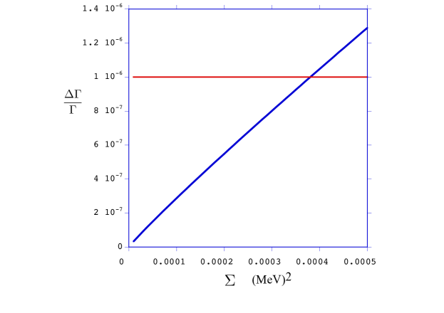
Figure 1: Plot of the theoretical percentage variation $\frac{\Delta\Gamma}{\Gamma}$ as a function of $\Sigma=m_{1}^{2}+m_{2}^{2}$ of Eq. (42).

The experimental value of the muon mean life is $\tau_{\mu}=(2.1969811\pm 0.0000022)$ [1] with a the relative uncertainty of the order of $10^{-6}$. In order to establish the neutrino mass interval compatible with the experimental uncertainty we must calculate the theoretical expression of $\frac{\Delta\Gamma}{\Gamma}$

$$\frac{\Delta\Gamma}{\Gamma}=\frac{\frac{\Sigma}{2m_{\mu}^{2}}(Q_{\Sigma a}+Q_{\Sigma b}~{}ln(\frac{2\Sigma}{m_{\mu}^{2}}))}{Q_{0}}\simeq\frac{\Sigma}{2m_{\mu}^{2}}(Q_{\Sigma a}+Q_{\Sigma b}~{}(\frac{2\Sigma}{m_{\mu}^{2}}))$$ (42)

and impose to be not greater than $10^{-6}$.

The plot of Fig. 1 shows that the uncertainty in $\Delta\Gamma/\Gamma$ is compatible with the experimental error in $\tau$, provided that

$$\Sigma=m_{1}^{2}+m_{2}^{2}<4~{}10^{-4}~{}MeV^{2}$$ (43)

Assuming [5] $m_{1}$ to be of the order $1~{}eV$, this implies that

$$m_{2}<0.02~{}MeV$$ (44)

an upper limit which is an order of magnitude stronger than the one reported in [1].

A similar result, namely $m_{2}<0.021~{}MeV$, has been obtained in [5] without imposing for $\Delta$ the value coming from the neutrino oscillation and observing within which interval the variation of $m_{2}$ is compatible with the corresponding experimental errors.

4 The helicity of the electron

We consider now the helicity of the final electron, defined as

$$h=\frac{d\Gamma(\uparrow)-d\Gamma(\downarrow)}{d\Gamma(\uparrow)+d\Gamma(\downarrow)}$$ (45)

where with $\uparrow$ ($\downarrow$) we mean that the electron momentum $\vec{p}$ is parallel (antiparallel) to the the spin vector $\vec{n}$.

In the case of unpolarized muon we get

$$h=\frac{(S_{0}+pS_{n})-(S_{0}-pS_{n})}{(S_{0}+pS_{n})-(S_{0}-pS_{n})}=\frac{pS_{n}}{S_{0}}$$ (46)

that is

$$h=-\frac{p}{E}\frac{W-2E+m_{\mu}+\frac{\Sigma}{2m_{\mu}}\frac{E-2W+m_{\mu}}{W-E}+\frac{\Delta^{2}}{4m_{\mu}^{2}}\frac{W+E-2m_{\mu}}{(W-E)^{2}}}{3W-2E-\frac{m_{e}^{2}}{E}+\frac{\Sigma}{2m_{\mu}}\frac{E-\frac{m_{e}^{2}}{E}}{W-E}+\frac{\Delta^{2}}{4m_{\mu}^{2}}\frac{E-3W+2\frac{m_{e}^{2}}{E}}{(W-E)^{2}}}$$ (47)

For massless neutrinos, the helicity $h_{0}$ is simply given by

$$h_{0}=-\frac{p}{E}\frac{W-2E+m_{\mu}}{3W-2E-\frac{m_{e}^{2}}{E}}$$ (48)

which increases with $E$ and starts to be about $-0.99$ already for energies $E\geq 3MeV$.

The introduction of finite neutrino masses do not alter significantly such value. In fact, the quantity

$$\frac{h-h_{o}}{h_{0}}$$ (49)

is at most of the order of $10^{-9}$ if the masses of the last section ($m_{1}=1~{}eV,m_{2}=0.02~{}MeV$) are used. Even if $m_{2}$ is chosen $10~{}MeV$, such value reaches scarcely $10^{-5}$. Considering that this neutrino mass is incompatible with the present experimental information and that the uncertainty in the measure of $h$ (and also of similar quantities) is of the order of percent, it is clear that the introduction of non zero neutrino masses, within the limits discussed in the last section, is perfectly compatible with phenomenology.

5 Energy and angular distribution of the electron

Let us consider the more general case in which both the electron and the $\mu$ meson are polarized. It is convenient to assume the $x$-axis parallel to the direction of the electron momentum $\vec{p}$ and the plane containing the electron momentum and the $\mu$ polarization vector $\vec{t}$ to be the $(x,y)$ plane . In this way we have

$$\vec{p}=(0,0,p)~{}~{}~{}~{}\vec{t}=(sin\theta,0,cos\theta)~{}~{}~{}~{}\vec{n}=(cos\psi~{}sin\phi,sin\psi~{}sin\phi,cos\phi)$$ (50)

and

$$(\vec{p}\cdot\vec{t})=pcos\theta~{}~{}~{}~{}(\vec{p}\cdot\vec{n})=pcos\phi$$ (51)

$$(\vec{n}\cdot\vec{t})=sin\theta~{}cos\psi~{}sin\phi+cos\theta~{}cos\phi~{}~{}~{}~{}(\vec{p}\cdot\vec{n})(\vec{p}\cdot\vec{t})=p^{2}cos\theta~{}cos\phi$$ (52)

Since there is no observation of the azimuthal angle of the electron momentum, we can say that the electron phase space $d^{3}p=EPdEd\Omega$ becomes $2\pi EPdEd(cos\theta)$ and the transition strength is given by

$$d\Gamma=\frac{G^{2}}{(2\pi)^{3}}\frac{m_{\mu}^{5}}{96}SPEdEd(cos\theta)$$ (53)

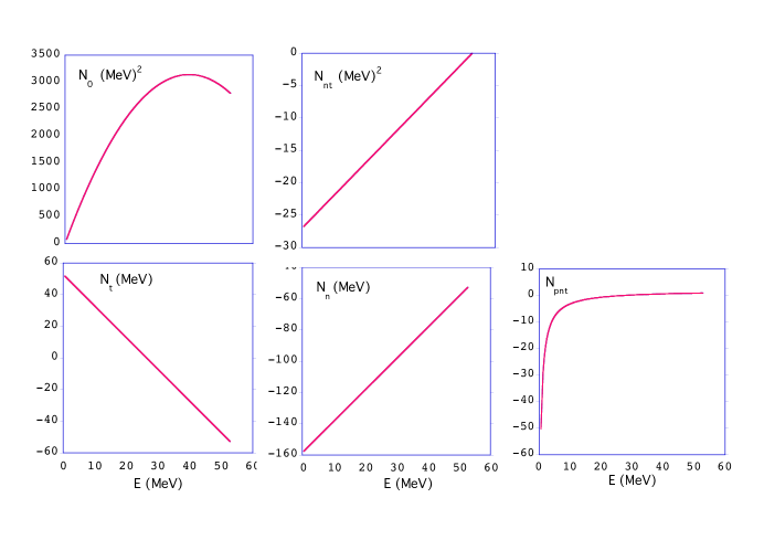
Figure 2: Plot of the various distributions $N_{0},N_{nt},N_{t},N_{n},N_{pnt}$ as functions of the electron energy $E$.

For later convenience we introduce the definition

$$S=\frac{32}{Em_{\mu}^{4}}N$$ (54)

and then

$$d\Gamma=\frac{G^{2}}{(2\pi)^{3}}\frac{m_{\mu}}{3}NPdEd(cos\theta)$$ (55)

with

$$N=N_{0}+N_{t}~{}\vec{p}\cdot\vec{t}+N_{n}~{}\vec{p}\cdot\vec{n}+N_{nt}~{}\vec{n}\cdot\vec{t}+N_{pnt}~{}\vec{p}\cdot\vec{t}~{}\vec{p}\cdot\vec{n}$$ (56)

and, according to Eqs. (30-34)

$$N_{0}=3WE-2E^{2}-m_{e}^{2}+\frac{\Sigma}{2m_{\mu}}\frac{E^{2}-m_{e}^{2}}{W-E}+\frac{\Delta^{2}}{4m_{\mu}^{2}}\frac{E^{2}-3WE+2m_{e}^{2}}{(W-E)^{2}}$$ (57)

$$N_{t}=W-2E+\frac{m_{e}^{2}}{m_{\mu}}+\frac{\Sigma}{2m_{\mu}}\frac{E-2W+\frac{m_{e}^{2}}{m_{\mu}}}{W-E}+\frac{\Delta^{2}}{4m_{\mu}^{2}}\frac{W+E-2\frac{m_{e}^{2}}{m_{\mu}}}{(W-E)^{2}}$$ (58)

$$N_{n}=-W+2E-m_{\mu}-\frac{\Sigma}{2m_{\mu}}\frac{E-2W+m_{\mu}}{W-E}-\frac{\Delta^{2}}{4m_{\mu}^{2}}\frac{W+E-2m_{\mu}}{(W-E)^{2}}$$ (59)

$$N_{nt}=-m_{e}[W-E-\frac{\Sigma}{m_{\mu}}+\frac{\Delta^{2}}{4m_{\mu}^{2}}\frac{1}{W-E}]$$ (60)

$$N_{pnt}=\frac{1}{(E+m_{e})}[2E-W+m_{e}+\frac{\Sigma}{2m_{\mu}}\frac{2W-E+m_{e}}{(W-E)}-\frac{\Delta^{2}}{4m_{\mu}^{2}}\frac{W+E+2m_{e}}{(W-E)^{2}}]$$ (61)

Using the value reported in Eq. (35), we can neglect the contributions containing the factor $\Delta$ in the above equations. Moreover for the neutrino masses we assume the upper values discussed in Sec. 3, namely $10^{-6}MeV$ and $0.02~{}MeV$ for the electron and $\mu$ cases, respectively.

The various distributions $N_{0},N_{nt},N_{t},N_{n},N_{pnt}$ as functions of the energy $E$ are reported in Fig. 2. As a matter of fact, in each sector both the curves with and without neutrino masses are plotted in Fig. 2, but they are practically coincident. The reason is that, because of the smallness of the neutrino masses and consequently of the factor $\frac{\Sigma}{2m_{\mu}}$, the percentage difference $\Delta N/N$, for all distributions, starts to reach values of the order of percent only for $E$ greater than $52.83~{}MeV$, which is quite close to the maximum electron energy of Eq. (26).

The situation is practically the same also if one determines $\Delta$ using the same masses as for $\Sigma$, even if in this case the denominator $(W-E)^{2}$ is more effective. Similarly, there is no noticeable change in the behaviour of the distributions $N$ if the upper value of $0.19~{}MeV$ [3] for the $\mu$ type lepton is used.

These facts show that the presence of two neutrino masses compatible with the beta decay [2] and the muon mean life [5] do not alter the energy and angular distribution of the emitted electron.

6 The leptonic decay of the $\tau$ meson

From the calculations made for the $\mu$ one can obtain the corresponding ones for the leptonic decay of the $\tau$ meson

$$\tau^{-}\rightarrow\mu^{-}+\bar{\nu}_{\mu}+\nu_{\tau}$$ (62)

with the following substitutions

$$m_{e}\rightarrow m_{\mu}~{}~{}~{}~{}m_{\mu}\rightarrow m_{\tau}~{}~{}~{}~{}m_{1}\rightarrow m_{2}~{}~{}~{}~{}m_{2}\rightarrow m_{3}$$ (63)

The results are substantially similar to the case of the $\mu$ decay. In particular, the $N$ distributions introduced n the preceding section are practically unaffected by the presence of the terms with non zero masses of the two neutrinos. Here again, the percentage difference $\Delta N/N$ starts to reach values of the order of percent only for $E$ very near to the maximum value, which is about $890~{}MeV$.

However, at variance with the $\mu$ decay, the experimental uncertainty of the $\tau$ mean life is not sufficiently small to allow an improvement of the upper value of the $\nu$ mass (tau based) [5].

Similar considerations are valid for the charge-conjugated decay

$$\tau^{+}\rightarrow\mu^{+}+\nu_{\mu}+\bar{\nu}_{\tau}$$ (64)

but also fore the other leptonic decay of the $\tau$ meson:

$$\tau^{-}\rightarrow e^{-}+\bar{\nu}_{e}+\nu_{\tau}$$ (65)

and its charge conjugated one.

7 Conclusions

The neutrino oscillationsare possible only if at least two neutrinos are massive, whereas in the Standard Model calculation only zero mass neutrinos are considered. In this paper it is shown to which extent massive neutrinos are compatible with the standard calculations of the $\mu$ decay. In fact, most of the observables in the $\mu$ decay are known with a not too high precision and the ensuing uncertainty is not able to exclude the presence of massive neutrinos of the electron and muon type, provided that their masses are not too high, that is within the upper limits reported in refs. [2, 3, 4] or, in the case of the muon based evaluation, the one obtained [5] taking advantage of the small error in the $\mu$ lifetime.

Similar considerations are valid also for the two leptonic decays of the $\tau$ meson, showing that, at least for purely leptonic weak decays, the presence of a non zero value for all three neutrinos does not alter the agreement between the standard calculations and the experimental data.

Appendix

Calculation of the integrals necessary for the determination of the mean life

The total width is (see Eq. (36))

$$\Gamma=\frac{G^{2}}{\pi^{3}192}m_{\mu}^{5}\int_{E_{min}}^{E_{max}}SpEdE=\frac{G^{2}}{\pi^{3}192}m_{\mu}^{5}Q$$ (66)

where $Q$ is given by

$$Q=\int_{E_{min}}^{E_{max}}S_{0}pEdE=$$ (67)

$$=\frac{32}{m_{\mu}^{4}}\int_{E_{min}}^{E_{max}}[3W-2E-\frac{m_{e}^{2}}{E}+\frac{\Sigma}{2m_{\mu}}\frac{E-\frac{m_{e}^{2}}{E}}{W-E}+\frac{\Delta^{2}}{4m_{\mu}^{2}}\frac{E-3W+2\frac{m_{e}^{2}}{E}}{(W-E)^{2}}]pdE=$$ (68)

$$=\frac{32}{m_{\mu}^{4}}[3WK_{0}-2K_{1}-m_{e}^{2}K_{2}+\frac{\Sigma}{2m_{\mu}}(K_{3}-m_{e}^{2}K_{4})+\frac{\Delta^{2}}{4m_{\mu}^{2}}(K_{5}-3WK_{6}+2m_{e}^{2}K_{7})]$$ (69)

having defined the integrals

$$K_{0}=\int_{E_{min}}^{E_{max}}EpdE,~{}~{}~{}~{}K_{1}=\int_{E_{min}}^{E_{max}}E^{2}pdE~{}~{}~{}~{}K_{2}=\int_{E_{min}}^{E_{max}}pdE,$$ (70)

$$K_{3}=\int_{E_{min}}^{E_{max}}dE\frac{E^{2}p}{W-E}dE~{}~{}~{}~{}K_{4}=\int_{E_{min}}^{E_{max}}\frac{p}{W-E}dE,$$ (71)

$$K_{5}=\int_{E_{min}}^{E_{max}}\frac{E^{2}p}{(W-E)^{2}}dE,~{}~{}~{}~{}K_{6}=\int_{E_{min}}^{E_{max}}\frac{pE}{(W-E)^{2}}dE$$ (72)

$$K_{7}=\int_{E_{min}}^{E_{max}}\frac{p}{(W-E)^{2}}dE$$ (73)

With the definitions

$$x=\frac{m_{e}^{2}}{m_{\mu}^{2}},~{}~{}~{}~{}Z_{m}=\frac{(m_{1}+m_{2})^{2}}{m_{\mu}^{2}}=\frac{2}{m_{\mu}}(W-E_{max})$$ (74)

we have

$$W=\frac{m_{\mu}}{2}(1+x),~{}~{}~{}~{}\sqrt{W^{2}-m_{e}^{2}}=\frac{m_{\mu}}{2}(1-x)$$ (75)

and the values of the integrals are

$$K_{0}=\frac{m_{\mu}^{3}}{24}(1-x)^{3}$$ (76)

$$K_{1}=\frac{m_{\mu}^{4}}{64}(1-x^{4}+4x^{2}~{}lnx)$$ (77)

$$K_{2}=\frac{m_{\mu}^{2}}{8}(1-x^{2}+2x~{}lnx)$$ (78)

$$K_{3}=\frac{m_{\mu}^{3}}{8}[-\frac{11}{6}-\frac{x}{2}+\frac{x^{2}}{2}+\frac{11}{6}x^{3}+2(1-x)(1+x)^{2}~{}ln(1-x)+x^{2}(1+x)~{}lnx+$$ (79)

$$-(1-x)(1+x)^{2}~{}lnZ_{m}]$$ (80)

$$K_{4}=\frac{m_{\mu}}{2}[-1+x+2(1-x)~{}ln(1-x)+x~{}lnx-(1-x)~{}lnZ_{m}]$$ (81)

$$K_{5}=\frac{m_{\mu}^{2}}{8}[5(1-x^{2})+2\frac{(1-x)(1+x)^{2}}{Z_{m}}+\frac{4(1+x)}{1-x}(-3+2x-3x^{2})~{}ln(1-x)+$$ (82)

$$+2\frac{x^{2}(1+3x)}{1-x}~{}lnx+2\frac{1+x}{1-x}(3-2x+3x^{2})~{}lnZ_{m}]$$ (83)

$$K_{6}=\frac{m_{\mu}}{2}[1-x+\frac{1-x^{2}}{Z_{m}}-4\frac{1+x^{2}}{1-x}~{}ln(1-x)+2\frac{x^{2}}{1-x}~{}lnx+2\frac{1+x^{2}}{1-x}~{}lnZ_{m}]$$ (84)

$$K_{7}=\frac{1-x}{Z_{m}}+\frac{1+x}{1-x}~{}lnZ_{m}-2\frac{1+x}{1-x}~{}ln(1-x)+\frac{x}{1-x}lnx$$ (85)

Introducing the parametrization

$$Q=Q_{0}+\frac{\Sigma}{2m_{\mu}^{2}}(Q_{\Sigma a}+Q_{\Sigma b}~{}lnZ_{m})+\frac{\Delta^{2}}{4m_{\mu}^{4}}(Q_{\Delta a}+Q_{\Delta b}~{}lnZ_{m}+\frac{Q_{\Delta c}}{Z_{m}})$$ (86)

we get the expressions reported in Table 1.