Improving Order with Queues

Abstract

A classic problem in computer science is the following: given a sequence of $n$ numbers, and a collection of $k$ parallel queues, can we sort this sequence with these $k$ queues? The queues operate on a First-In-First-Out (FIFO) principle. We can push the elements of the input sequence, one by one, into the queues, and construct the output sequence by popping elements from the queues, one by one. This problem was studied by Tarjan, inspired by a problem posed by Knuth. It was studied in the context of certain card games (Patience and Floyd’s game), which led to an algorithm called Patience sort for it. Evan and Itai related it to chromatic number of Permutation graphs. It also arises in the context of planning and sorting items in assembly lines of factories, which has important applications.

We call the length of the Longest Decreasing Subsequence of a sequence its LDS. It is known that $k$ queues suffice if and only if the LDS of the input sequence is at most $k$. In this paper, we consider this problem when the number of queues $k$ is given and the LDS of the input sequence is possibly more than $k$. This is a natural generalization that appears in some important practical applications. Surprisingly, not much is known about it. We investigate the extent to which the disorder of the input sequence can be reduced. We prove the following results:

1. Let $L$ be the LDS of the input sequence. We give a simple algorithm that, using $k$ queues, reduces the LDS from $L$ to $L-k+1$. It is based on Patience sort.

2. Then we show that, for any $L>0$, there exist sequences of LDS $L$, such that it is impossible to reduce the LDS below $L-k+1$ with only $k$ queues. Thus, the above algorithm is optimal. This completely characterizes the power of $k$ parallel queues in reducing the LDS and is the first main result of this paper.

3. Sorted sequences have LDS $1$. Merging two sorted queues to produce a sorted sequence is a central step in efficient sorting algorithm, and it is always possible. In contrast, we show that if the two sequences have LDS $2$, then it is not always possible to merge them into a sequence of LDS $2$. Indeed, we give an algorithm that given two sequences of LDS $2$, decides in polynomial time if it is possible to merge them.

4. Following the above barriers on LDS, we consider an alternative measure of disorder in a permutation, namely the number of downsteps. A downstep in a sequence is an item immediately followed by a smaller item. Intuitively, it represents a ‘hiccup’ in the sequence. We give an algorithm that for any number $k$ of queues, outputs a sequence with the least number of down-steps attainable with $k$ queues. This algorithm is online. This completely characterizes the power of $k$ parallel queues in reducing downsteps and is the second main result of our paper.

Our research was inspired by an application in car manufacturing.

None

1 Introduction

A classic problem in computer science is the following: Given a sequence $\pi$ of $n$ numbers, and a collection of $k$ parallel queues, can we sort $\pi$ using these queues? Queues operate on a First-In-First-Out(FIFO) principle. The elements of $\pi$ are, one by one, pushed into one of the $k$ queues, and the output sequence is generated by popping elements from one of the $k$ queues, one-by-one.

This problem was studied by Tarjan [20] inspired by a problem posed by Knuth [13], and also by Even and Itai [9]. It was studied even earlier by Schensted [18], and later by Mallows [14] in context of certain card games (Patience and Floyd’s game). It is known that we can sort $\pi$ if and only if the number of queues, $k$, is at least the length of the longest decreasing subsequence(LDS) of $\pi$ [20]. It can achieved by using an algorithm called Patience sort [1]. This problem is related to the chromatic number of the Permutation graphs [11, 9]: the length of the LDS of $\pi$ is equal to the chromatic number of a certain conflict graph of $\pi$, which is a permutation graph. It is also related to certain properties of the Young Tableaux [18, 1].

A particularly important application of this problem appears in factories, where items are produced on assembly lines. Assembly lines, e.g., in car manufacturing, are partitioned by buffers to minimize the effect of line stops in one section to the other ones. The simplest buffer consists of a single lane that operates as a queue according to the First-In-First-Out (FIFO) principle, which maintains the order in which the items arrive and leave. Typically, there are two or more parallel lanes to which the arriving items are distributed and the leaving sequence is merged from. This presents a mechanism of buffers with sorting capabilities depending on the number of parallel queues it consists of. More sorting power allows more flexibility in the the planning of the build sequence because different sections may have other constraints and/or objectives [15, 5, 19, 8]. Moreover, displacements in the sequence, e.g., caused by faults or other real-world events, can be mitigated to some extent as well. Understanding the sorting capabilities of such buffer mechanisms becomes very important in these applications.

Patience sort [1], a sorting algorithm inspired by the card game Patience, sorts a sequence of numbers using a minimal number of queues. The input is a sequence $\pi_{1}$ to $\pi_{n}$ of $n$ distinct numbers and the goal is to sort the numbers into increasing order. One starts with a set of empty queues $Q_{1}$, $Q_{2}$, … and then enqueues the numbers one by one. When $\pi_{i}$ is to be enqueued one determines the smallest index $j$ such that either $\pi_{i}$ is larger than the last element in the $j$-th queue or the $j$-th queue is empty and then appends $\pi_{i}$ to the $j$-th queue. In this way, an increasing sequence is constructed in each queue . Once all elements are enqueued, the sorted sequence is extracted by repeatedly dequeuing the smallest first element of any queue. We call this dequeuing strategy Smallest Element First for later reference. The number of queues required by Patience Sort is the length of the longest decreasing subsequence in the input sequence and no algorithm can sort with fewer queues. Moreover, if one considers all permutations of a sorted sequence that can be sorted again using a certain number of queues, say $k$, this yields the set of permutations avoiding the pattern $(k+1,k,\ldots,1)$.

In this paper we ask: What can one do if the number of queues is fixed and may be smaller than the length of the longest decreasing subsequence of the input? This is a natural generalization, with some important practical applications, and also an interesting combinatorial problem in it’s own right. Surprisingly not much was known about it.

Our investigations lead us to consider: How does one measure the “disorder” of a sequence and how much of it can one remove with $k$ queues? We will consider two measures of disorder:

• The length of the longest decreasing subsequence of a sequence

• The number of down-steps in a sequence, i.e., the number of elements that are immediately followed by a smaller element.

Let $k$ be the number of available queues, $n$ be the length of the input sequence and $L$ be the LDS of this sequence. It is easy to observe that the LDS is $1$ if and only if the number of downsteps is $0$; which happens only for sorted sequences. Observe that, in general, the number of downsteps of a sequence is always at least as large as the LDS minus one; this follows directly from the properties of a longest decreasing subsequence. On the other hand, there exist sequences of length $n$, where the number of downsteps is $n/2$ while the LDS is just $2$, e.g., $2,1,4,3,\ldots,n,n-1$.

For LDS, we first give a simple algorithm based on Patience Sort that reduces the LDS from $L$ to $L-k+1$. It can be considered as a truncated Patience Sort and runs in time $O(n\log k)$.

Theorem 1.1.

Let $L\geq 1$ be arbitrary. With $k$ queues the LDS of any sequence with LDS $L$ can be reduced to $L-k+1$. The algorithm can be made to run in time $O(n\log k)$, where $n$ is the length of the input sequence.

On the other hand, the LDS cannot be reduced below $L/k$ as at least one of the queues must contain at least that many elements from an LDS of the input and elements in the same queue cannot overtake each other. This lower bound suggests a natural strategy: distribute the elements of the input sequence to the $k$ queues s.t. the LDS of each queue is at most $\lceil L/k\rceil$ and then merge these sequences optimally. To this end, we consider the question of merging two queues without increasing the LDS. In this context, recall that merging two sorted lists to produce another sorted list is central to efficient sorting algorithms, such as Mergesort [7]. The LDS of a sorted list is $1$. It is folklore that we can always merge two queues of LDS $1$ to produce a sequence of LDS $1$. But what happens if the the two queues have LDS $2$ or more?

We show that, there exist two sequences of LDS $2$ that cannot be merged to a sequence of LDS of $2$. We further give an algorithm that, given two sequences of LDS $2$, either merges them into a sequence of LDS $2$, or correctly concludes that they can’t be merged. This is accomplished via a reduction to the $2$-SAT problem.

Theorem 1.2.

There exist two sequences of LDS $2$ such that they can’t be merged into a sequence of LDS $2$.

Further, there is an algorithm that given two sequences of LDS $2$, either merges them into another sequence of LDS $2$, or correctly concludes that this is impossible. It can be implemented to run in linear time in $n$, the sum of the length of the two input sequences.

Based on this insight, we asked ourselves whether there is an algorithm that partitions a given an input sequence with LDS $4$ into two mergeable sequences. We found out that this is not always possible. We prove even more generally that for every integer $L$, there exists a sequence LDS $L$ such that it is impossible to reduce the LDS to strictly less than $L-k+1$ with only $k$ parallel queues. Hence, the above simple algorithm is tight, and no other other algorithm (no matter the running time) can do better! This lower-bound is unconditional and it is proved via a novel recursive construction. It completely characterizes the power of $k$ parallel queues in reducing the LDS of a sequence.

Theorem 1.3.

For every $L$, there exist sequences of LDS $L$ which cannot be improved to an LDS strictly less than $L-k+1$ with only $k$ parallel queues.

The above barriers on LDS motivated us to consider the second measure of disorder of a sequence, namely the number of down-steps. Recall that this is the number of items in the sequence that are immediately followed by a smaller item. Intuitively, each down-step represents a ‘hiccup‘ in the sequence, and our objective is to minimize these.

We give an optimal algorithm $\sf{Alg}_{\mathrm{DS}}$ for decreasing the number of down-steps, i.e., no algorithm can output a sequence with fewer down-steps than $\sf{Alg}_{\mathrm{DS}}$ does. The algorithm is online, i.e., the decision where to enqueue a particular element $\pi_{i}$ does not depend on the elements after $\pi_{i}$ in the input sequence. Further, it is essentially the unique optimal on-line algorithm in the sense that if any other on-line algorithm $\sf A$ deviates from $\sf{Alg}_{\mathrm{DS}}$ at any step, then there is a continuation of the sequence for which $\sf A$ produces an output with more down-steps than $\sf{Alg}_{\mathrm{DS}}$. The algorithm runs in time $O(n\log k)$, where $n$ is the length of the input sequence and $k$ is the number of available queues. It completely characterizes the power of $k$ parallel queues in reducing the number of downsteps.

Theorem 1.4.

There is an algorithm $\sf{Alg}_{\mathrm{DS}}$ that constructs an output sequence with a minimum number of down-steps. It is an on-line algorithm and can be implemented in (total) time $O(n\log k)$. Further, if any other online algorithm $\sf A$ deviates from $\sf{Alg}_{\mathrm{DS}}$, the input sequence can be extended such that $\sf A$ does strictly worse than $\sf{Alg}_{\mathrm{DS}}$.

Our Motivation and Related Results

Our research was motivated by an application in car manufacturing. The production in a car factory consists of three main stages: body (welding of the body), paint (painting the body), and assembly (adding engines, seats, …). Nowadays, cars can be configured in many different variants (different colors, different engines, different interiors, different entertainment systems, different sensors, …) and the sequence of cars passing through the production process must satisfy constraints of the factory floor and machinery. For example, no two subsequent cars may have the largest engine, only one out of three subsequent cars may have a roof-top, color changes cost money, and so on. Planning a sequence violating a (near) minimum number of constraints is presently an art [10, 16, 21].

Even if a sequence obeying all constraints is available at the beginning of the production process, this sequence will in general be perturbed in body and paint, e.g., because a welding point is not perfect and needs to be redone or the paint is not perfect and needs to be retouched. For this reason, there are buffers between body and paint and paint and assembly where the perturbed sequence can be improved to satisfy more constraints. In some factories, these buffers consist of a set of queues. This leads to our research question: “How much disorder can one remove using a given set of queues?” Surprisingly, we could not find any literature that addresses this problem for the two measures of order, i.e., LDS and number of downsteps, considered by us.

Boysen and Emde [5] study a closely related problem under the name parallel stack loading problem (PSLP). They consider only the enqueuing phase and the goal is to minimize the total number of down-steps in all queues. They also show that miminizing the number of down-steps in the enqueued sequences is NP-complete if the queue lengths are bounded; [3] gives an alternative NP-completeness proof. Gopalan et al. [12] studies a streaming algorithm with the goal to approximately miminize the number of edit-operations required for transforming an input sequence into a sorted sequence. This measure is also called the Ulam metric. For a sequence of length $n$, this measure is $n$ minus the length of the longest decreasing subsequence. Parallel algorithms for computing the edit and the Ulam distance are given by Boroujeni et al. [4]. Aldous and Diaconis[1] discuss the many interesting properties of patience sort. Chandramouli et al. [6] give a high-performance implemention of patience sort for almost sorted data.

Organization of the paper

In Section 2, we present proofs of Theorem 1.2 and Theorem 1.3. Then in Sections 3 we present a proof of Theorem 1.4. We then conclude in Section 4 with a few open problems.

2 The Longest Decreasing Subsequence

We begin with the first measure of disorder of a sequence, namely the length of the longest decreasing subsequence (LDS). We are interested in the following question:

How much can one reduce the LDS of a sequence using $k$ parallel queues?

We first present a simple algorithm based on Patience sort [1], that reduces the LDS from $L$ to $L-k+1$. Then, in Section 2.4, for each integer $L$, we give a construction of sequences of LDS $L$ such that it is impossible to reduce their LDS to strictly less than $L-k+1$ with $k$ queues. And finally in Section 2.2, we consider the related question of mergeability of two sequences of LDS $2$ or more.

2.1 Reducing LDS via Patience Sort

Theorem 2.1.

There is an algorithm that using $k$ queues reduces the LDS of a sequence from $L$ to $L-k+1$. The algorithm runs in $O(n\log k)$ time.

Proof 2.2.

Let us name these queues $Q_{1},Q_{2},\ldots,Q_{k}$. We place the elements of the input sequence into the $k$ queues such that the first $k-1$ queues have LDS $1$, and the last queue has LDS $L-k+1$. This can be done by simulating Patience sort using $L$ virtual queues $Q^{\prime}_{1},Q^{\prime}_{2},\ldots Q^{\prime}_{L}$, and sending the elements from $Q^{\prime}_{i}$ to $Q_{i}$ for $i\in[k-1]$, and sending the elements of $Q^{\prime}_{k},\ldots,Q^{\prime}_{L}$ to $Q_{k}$. The LDS of $Q_{k}$ is $L-k+1$ since it can be sorted using $L-k+1$ queues, namely $Q^{\prime}_{k}$, $\ldots$, $Q^{\prime}_{L}$.

Let us have a closer look at $Q_{k}$. Let $x$ and $y$ be consecutive elements in $Q^{\prime}_{k}$. Then all elements in $Q_{k}$ between $x$ and $y$ are smaller than $x$ as an element larger than $x$ would have been added to one of the queues $Q^{\prime}_{1}$ to $Q^{\prime}_{k}$.

We now merge the queues $Q_{1}$ to $Q_{k}$ using the Smallest Element First strategy. We claim this merges $Q^{\prime}_{1},\ldots,Q^{\prime}_{k}$ to an increasing sequence $S$, thus, yielding an output that can be partitioned into $L-k+1$ increasing sequences, namely $S$ and $Q^{\prime}_{k+1}$ to $Q^{\prime}_{L}$. Indeed, assume we have just output an element $x$ in $Q^{\prime}_{k}$ from $Q_{k}$ and let $y$ be the next element from $Q^{\prime}_{k}$ in $Q_{k}$. Then the first elements of $Q_{1}$ to $Q_{k-1}$ are larger than $x$ and all elements in $Q_{k}$ before $y$ are smaller than $x$. Thus they will be output next until $y$ is at the front of $Q_{k}$. Now the merge of $Q_{1}$ to $Q_{k}$ will continue in the same way as a merge of $Q^{\prime}_{1}$ to $Q^{\prime}_{k}$ until $y$ is dequeued.

The running time of the algorithm is $O(n\log k)$, which follows from Patience sort because the tails of the queues always form a decreasing sequence and the right queue can be found using binary search [1].

The above algorithm is very simple. It is natural to ask whether a more sophisticated algorithm can give better results perhaps by better balancing the LDS of the queues because the LDS in the output cannot be smaller than the maximum LDS over the $k$ queues. For example, this could be done by putting into $Q_{i}$, $i\in[k]$, all elements from $Q^{\prime}_{j}$ for each $j\in[L]$ with $j\equiv i\mod k$. Then, the LDS of each of $Q_{1},\ldots,Q_{k}$ is at most $\lceil L/k\rceil$.

We would then also have to look at a different merging strategy as Smallest Element First does not always yield the optimum merge as the following example shows. Consider $k=2$ and the input sequence $5,4,1,3,2$ with LDS $L=4$. The modulo procedure described above yields the two queues

$$Q_{1} :5,1,3 Q_{2}:4,2$$

and Smallest Element First merges them to $4,2,5,1,3$ with LDS $3$. However, we can also obtain $4,5,1,2,3$ with LDS $2$, which is optimal as both queues have LDS $2$ and at least one of the two queues must have an LDS of at least $L/k$.

Using two queues, two sequences of LDS two can always be merged into a sequence of LDS three (Theorem 2.1) and maybe into a sequence of LDS two (the preceding example). In the next section, we show that two cannot always be obtained and derive an optimal merging strategy. We leave it as an open problem to generalize this result to more than two queues or larger LDS.

2.2 Mergeability of sequences

Merging two (or more) sorted sequences of numbers is central to all efficient sorting algorithms such as Mergesort [7]. Given $k$ queues, each containing a sorted sequence of numbers, we can always merge them to output a sorted list of all the numbers by the Smallest Element First strategy. The LDS of a sorted list is $1$, and it is always possible to merge two (or more) queues of LDS $1$ into an output sequence of LDS $1$. Consider a generalization, where the LDS of the queues is $\ell>1$. Then, is it always possible to merge them into an output sequence of LDS $\ell$ ?

The answer to this question is no. Indeed, even for $2$ queues of LDS $2$ it is not possible, as illustrated by the following example:

$$Q_{1}:7,1,9,3\leavevmode\nobreak\ \leavevmode\nobreak\ \leavevmode\nobreak\ \leavevmode\nobreak\ \leavevmode\nobreak\ \leavevmode\nobreak\ \leavevmode\nobreak\ Q_{2}:4,2,5,8,6$$

It can be shown that any merging of these two queues will produce a sequence of LDS at least $3$. In this section, we present a more general result: We give an algorithm that, given 2 queues of LDS 2, either merges them into a sequence of LDS $2$, or correctly decides that they cannot be merged. We use the example above to illustrate it.

We have two sequences $Q_{1}$ and $Q_{2}$ each of LDS at most two. We want to decide whether $Q_{1}$ and $Q_{2}$ can be merged into a sequence of LDS at most two. A down-pair in a sequence is a pair $a,b$ with $a>b$ and $a$ preceding $b$ in the sequence.

We will define a precedence graph on the elements of $Q_{1}$ and $Q_{2}$. There are two kinds of edges. Strict edges and tentative edges. A strict edge $x\rightarrow y$ indicates that $x$ must be before $y$ in the output. Tentative edges come in pairs that share a common element. If $b\dashrightarrow e\dashrightarrow a$ are a pair of tentative edges then either $b$ must be before $e$ or $e$ must be before $a$ in the output; so the arrangement $a,e,b$ is forbidden.

In a sequence of LDS at most two, we have three kinds of elements: Left elements in a down-pair, right elements in a down-pair, and elements that are in no down-pair. We call such elements solitaires. Note that no element can be a left and a right element in a down-pair as this would imply a decreasing sequence of length three. For a solitaire, all preceding elements are smaller and all succeeding elements are larger. We have the following precedence edges.

1. For each sequence, we have the edges $x\rightarrow y$ if $x$ precedes $y$ in the sequence.

2. Assume $a,b$ is a down-pair in one of the sequences and $c,d$ is a down-pair in the other sequence. We have the edges $\min(a,c)\rightarrow\max(a,c)$ and $\min(b,d)\rightarrow\max(b,d)$.

3. Between two solitaires there are no constraints.

4. Assume $a,b$ is a down-pair in one of the sequences and $e$ is a solitaire in the other. We generate enough edges so that the elements cannot form a decreasing sequence of length 3.

   1. If $e>a$, then $a\rightarrow e$.

   2. If $e<b$, then $e\rightarrow b$.

   3. If $a>e>b$, then we have the pair $e\dashrightarrow a$ and $b\dashrightarrow e$ of tentative edges. We call them companions of each other. An edge may have many companions. For example, if $a,b$ and $a^{\prime},b$ are down-pairs with $a>e>b$ and $a^{\prime}>e>b$, $e\dashrightarrow a$ and $e\dashrightarrow a^{\prime}$ are companions of $b\dashrightarrow e$. Similarly, if $a,b$ and $a,b^{\prime}$ are down-pairs with $a>e>b$ and $a>e>b^{\prime}$, $b\dashrightarrow e$ and $b^{\prime}\dashrightarrow e$ are companions of $e\dashrightarrow a$.

      Tentative edges only end in solitaires or left endpoints.

Lemma 2.3.

If the output sequence obeys all strict edges and one tentative edge of each pair of tentative edges, the output sequence has LDS at most two.

Proof 2.4.

A decreasing subsequence of length three must consist of a down-pair $a,b$ from one of the sequences and an element $e$ from the other sequence; $e$ is either a solitaire or part of a down-pair $c,d$ with $e\in\{c,d\}$.

Assume first that $e$ is a solitaire. If $e>a$, we have the edge $a\rightarrow e$, if $b>e$ we have the edge $e\rightarrow b$, and if $a>e>b$, we have the pair of tentative edges $b\dashrightarrow e\dashrightarrow a$. In either case, it is guaranteed that the three elements do not form a decreasing sequence of length three.

Assume next that $e$ is part of a down-pair $c,d$. We will argue that the generated edges guarantee that the four elements $a,b,c,d$ do not produce a decreasing sequence of length three in the output. We have the edges $a\rightarrow b$ and $c\rightarrow d$, $\min(a,c)\rightarrow\max(a,c)$ and $\min(b,d)\rightarrow\max(a,d)$. Assume w.l.o.g. $a>c$. Then we have the edge $c\rightarrow a$. If $b>d$, we also have the edge $d\rightarrow b$ and hence the two possible interleavings are $c,a,d,b$ and $c,d,a,b$. Since $c$ precedes $a$ and $d$ precedes $b$, a decreasing sequence can contain at most one of $a$ and $c$ and at most one of $b$ and $d$. Thus its length is at most two. If $d>b$, we have the edge $b\rightarrow d$ and hence the only arrangement is $c,a,b,d$. Since $c$ precedes $a$ and $b$ precedes $d$, a decreasing sequence can contain at most one of $a$ and $c$ and at most one of $b$ and $d$. Thus its length is at most two.

We next give an algorithm for merging two sequences. The algorithm always considers the elements at the front of the two queues and decides which one to move to the output. It may also decide that the two sequences cannot be merged. If a front element is moved to the output, all edges incident to the element are deleted and the companions of all outgoing tentative edges are deleted. We call a front element of a sequence free if it has no incoming edge, blocked if is has an incoming strict edge, and half-free if there is an incoming tentative edge, but no incoming strict edge. Here are the rules.

1. If only one of the front elements is free, move it. If both front elements are free, move the smaller one.

2. If both front elements are blocked, declare failure.

3. If one front element is blocked and the other one is half-free, move the half-free and turn the companion edges of the incoming tentative edges into strict edges.

4. If both front elements are half-free, move the smaller one. Turn the companion edges of the incoming tentative edges into strict edges.

Figure 1 illustrates the algorithm on the example from the beginning of the section.

Lemma 2.5.

If the algorithm runs to completion, the output sequence obeys all strict edges and one of the tentative edges in each pair of tentative edges and hence the output has LDS at most two.

Proof 2.6.

All strict edges are obeyed since blocked elements are never moved to the output. Also, one edge of each pair of tentative edges is realized. This can be seen as follows. When we move an element to the output all outgoing tentative edges are realized and hence we may remove their companions. When we move a half-free element to the output, the incoming tentative edges are not realized. We compensate for this by making their companions strict.

Lemma 2.7.

If the algorithm fails, the two sequences cannot be merged.

Proof 2.8.

We assume that we start with two sequences that can be merged and consider the first moment of time when the algorithm makes a move that destroys mergeability. Let $e$ and $f$ be the heads of the queues before the move of the algorithm. The algorithm moves $e$ to the output, but the only move that maintains mergeability is moving $f$. Then $e$ is not blocked as the algorithm moves it.

Claim 1.

$f$ is not blocked.

Assume $f$ is blocked. Then there is a strict edge $a\rightarrow f$ from an element $a$ in $e$’s queue. The strict edge was either created as a strict edge or was created as a tentative edge and later turned into a strict edge.

Assume first that either $a$ or $f$ is a solitaire. If the edge was created as a strict edge and $f$ is a solitaire, then $f>a$ and $a$ is the left element of a down-pair $a,b$. The decreasing sequence $f,a,b$ will be created, a contradiction. If the edge was created as a strict edge and $a$ is a solitaire, then $f>a$ and $f$ is the right element of a down-pair $g,f$. The decreasing sequence $g,f,a$ will be created. If the edge was created as a tentative edge and $f$ is a solitaire, then there is a down-pair $a^{\prime},a$ in $e$’s input sequence with $a^{\prime}>f>a$ and we had the tentative edges $a\dashrightarrow f\dashrightarrow a^{\prime}$. Since the edge $a\dashrightarrow f$ is now a solid edge, $a^{\prime}$ was already moved to the output. Thus the decreasing sequence $a^{\prime},f,a$ will be created. If the edge was created as a tentative edge and $a$ is a solitaire, then there is a down-pair $f,f^{\prime}$ in $f$’s input sequence with $f>a>f^{\prime}$ and we had the tentative edges $f^{\prime}\dashrightarrow a\dashrightarrow f$. Since $f^{\prime}$ is after $f$ in $f$’s input sequence, the tentative edge $a\dashrightarrow f$ is still there as a tentative edge.

We come to the case that $a$ and $f$ are elements of down-pairs. Then either both are left elements or both are right elements in their down-pairs, as we do not create edges (neither strict nor tentative) between left and right endpoints of down-pairs. Also, $a<f$ since edges always go from the smaller element to the larger element. If both are left elements and $a,b$ is a down-pair with $a$ on the left, the decreasing sequence $f,a,b$ will be created. If both are right elements and $g,f$ is a down-pair with $f$ on the right, the decreasing sequence $g,f,a$ will be created.

We have now shown that a blocked element should never be moved to the output.

So we have to consider four cases depending on which of $e$ and $f$ are free or half-free.

Let $C=P\,f\,Q\,e\,R$ be a correct merging; here $P$, $Q$ and $R$ are sequences. We want to argue that $M=P\,e\,f\,Q\,R$ is also a correct merging. Assume otherwise. Then there must be a decreasing sequence of length 3 in $M$. As this decreasing sequence does not exist in $C$, it must involve $e$. All elements in $Q$ come from $f$’s queue as no element from $e$’s queue can overtake $e$ in $C$.

If the decreasing subsequence in $M$ does not involve $f$ (this is definitely the case if $e<f$), it must contain an element from $Q$, say $y$, as otherwise it would also exist in $C$.

If $f>e$, all elements in $P$ must be smaller than $f$ and all elements in $R$ must be larger than $e$, as otherwise $C$ would contain a decreasing subsequence of length 3.

$e$ and $f$ are free: We have $e<f$ since the algorithm moves $e$. So the decreasing sequence cannot contain $f$. Also, $e$ cannot be the first element of the decreasing sequence as otherwise replacing the first element by $f$ would result in a decreasing sequence of length 3 in $C$. It cannot be the last element of the decreasing sequence as the sequence contains an element of $Q$. So the decreasing sequence has the form $x\,e\,y$ with $x$ in $P$ and $y$ in $Q$. Since $f>e>y$, $f,y$ is a down-pair in $f$’s sequence. If $e$ is a solitaire, we have the tentative edge $e\dashrightarrow f$ (Rule d3) and hence $f$ is not free, a contradiction. If $e$ is the left element in a down-pair, we have a strict edge $e\rightarrow f$ (Rule b1), a contradiction. If $e$ is the right element in a down-pair, we have the strict edge $y\rightarrow e$, a contradiction (Rule b1)

$e$ is free and $f$ is half-free: Since $f$ is half-free, there is a tentative edge $d\dashrightarrow f$ from an element $d$ in $e$’s queue. Thus $f$ is a solitaire or a left endpoint.

If $f$ is a solitaire, there is a down-pair $c,d$ in $e$’s sequence with $c>f>d$; $d$ is still in $e$’s queue. If $e<f$, the decreasing sequence has the form $x\,e\,y$ with $x$ in $P$ and $y$ in $Q$ by the same argument as in the first case. Recall that all elements in $Q$ come from $f$’s queue. Thus $f,y$ is a down-pair, a contradiction to $f$ being a solitaire. If $e>f$, $e,d$ is a down-pair with $e>f>d$. Thus, we have the tentative edge $f\dashrightarrow e$ (Rule d3) and $e$ is not free, a contradiction.

If $f$ is a left endpoint, $d$ is a solitaire in $e$’s sequence. We have $f>d$. Since $d$ is a solitaire, we have $e<d$ and hence $e<f$. By the same argument as in the first case, the decreasing sequence has the form $x\,e\,y$ with $x$ in $P$ and $y$ in $Q$. Thus $f,y$ is a down-pair with $f>d>e>y$. If $e$ is a left endpoint, we have the strict edge $e\rightarrow f$ (Rule b1) and $f$ is blocked. If $e$ is a right endpoint, we have the strict edge $y\rightarrow e$ (Rule b1) and $e$ is not free. If $e$ is a solitaire, we have the tentative edges $y\dashrightarrow e\dashrightarrow f$ (Rule d3) and $e$ is not free. In either case, we derived a contradiction.

$e$ is half-free and $f$ is free: This case cannot arise, as the algorithm would move $f$.

$e$ and $f$ are half-free: We have $e<f$, since the algorithm moves $e$. By the same argument as in the first, case, the decreasing sequence has the form $x\,e\,y$ with $x$ in $P$ and $y$ in $Q$.

$f,y$ is a down-pair in $f$’s sequence. If $e$ is the left element in a down-pair, we have a strict edge $e\rightarrow f$ (Rule b1), a contradiction. If $e$ is the right element in a down-pair, we have the strict edge $y\rightarrow e$ (Rule b1), a contradiction.

If $e$ is a solitaire, all elements in $P$ that come from $e$’s queue are smaller than $e$ and all elements in $R$ are larger than $e$. This implies that $x$ comes from $f$’s queue and precedes $f$ in its input sequence, and hence $x,y$ is a down-pair in $f$’s queue with $x>e>y$. So we have the tentative edges $y\dashrightarrow e\dashrightarrow x$ (Rule d3). When $x$ was moved to the output, the tentative edge $y\dashrightarrow e$ was converted to a strict edge, a contradiction.

If there are no solitaires, the algorithm greatly simplifies. All edges of the precedence graph are strict and we have mergeability if and only if the precedence graph is acyclic. A cycle in the precedence graph is a short certificate for non-mergeability. In the presence of solitaires we have pairs of tentative edges and the question is whether there is a choice of tentative edges, one from each pair of tentative edges, such that the resulting graph is acyclic or whether for any choice the graph is cyclic. We next show how to formulate this question as a 2-SAT problem.

Let us use $q_{1}q_{2}\ldots q_{n}$ and $p_{1}p_{2}\ldots p_{m}$ to denote the two input sequences. The edges defined by our rules b) and d) run between the two input sequences. For each such edge we have a variable $x_{e}$: $x_{e}=\mathrm{true}$ if the output realizes $e$ and $x_{e}=\mathrm{false}$ otherwise. We say that two edges $q_{h}p_{i}$ and $p_{j}q_{k}$ cross iff $i<j$ and $k<h$ or $i=j$ and $h=k$. If there are crossing strict edges, we have non-mergeability. We have the following clauses.

• For each strict edge $e$, the singleton clause $x_{e}$.

• For each companion pair $e$ and $e^{\prime}$ of tentative edges, $x_{e}\vee x_{e^{\prime}}$ and $\neg x_{e}\vee\neg x_{e^{\prime}}$

• For each pair of crossing edges $e$ and $e^{\prime}$, $\neg x_{e}\vee\neg x_{e^{\prime}}$.

Strict edges must be realized. From each pair of companion edges exactly one has to be realized. From each pair of crossing edges at most one should be realized. Let $F$ be the conjunction of the clauses defined above.

Lemma 2.9.

$F$ is satisfiable if and only if the two sequences are mergeable.

Proof 2.10.

Assume $F$ is satisfiable. Let $E$ be the set of edges corresponding to true variables; $E$ includes all strict edges, exactly one out of each pair of tentative edges, and at most one edge in each pair of crossing edges. Add the edges $q_{i}q_{i+1}$ for $1\leq i<n$ and $p_{j}p_{j+1}$ for $1\leq j<m$. The resulting graph is acyclic. Assume otherwise and let $q_{i}$ and $p_{j}$ be the elements with minimum index in a cycle. Then there must be an edge $p_{h}q_{i}$ with $h>j$ and $q_{k}p_{j}$ with $k>i$ or with $i=k$ and $j=h$. So we have a pair of realized crossing edges which is impossible.

Assume conversely that the sequences are mergeable. Then all strict edges are realized and exactly one out of each companion pair of tentative edges is realized. Set the variables corresponding to realized edges to true. Then the first two types of clauses are certainly true. The third type is also true since in a pair of crossing edges at most one can be realized.

For 2-SAT formulae there are simple witnesses of satisfiability and non-satisfiability [2], computable in polynomial time. We briefly review the argument. A satisfying assignment is a witness for satisfiability. For a witness of non-satisfiability, write all clauses involving two literals as two implications, i.e., replace $x\vee y$ by $\neg x\rightarrow y$ and $\neg y\rightarrow x$. Clearly, all singleton clauses need to be satisfied. Do so and follow implications. If this leads to a contradiction, the formula is not satisfiable, and we have a witness of the form $x\rightarrow^{*}y$ and $x^{\prime}\rightarrow^{*}\neg y$ for two singleton clauses $x$ and $x^{\prime}$ and a literal $y$. After this process there are no singleton clauses. Create a graph with the literals as the nodes of the graph and the implications as the directed edges. If there is a cycle containing a variable and its complement, the formula is not satisfiable. So assume otherwise. Consider any variable $x$. We may have the implication $x\rightarrow^{*}\neg x$ or the implication $\neg x\rightarrow^{*}x$ but we cannot have both as we would have a cycle $x\rightarrow^{*}\neg x\rightarrow*x$ involving $x$ and $\neg x$. If we have only the former, set $x$ to false, if we have only the latter, set $x$ to true, if we have neither, set $x$ to an arbitrary value. Follow implications. This cannot lead to an contradiction. Assume we have the implication $x\rightarrow^{*}\neg x$ and hence set $x$ to false and $\neg x$ to true. If this would lead to a contradiction, we would have implications $\neg x\rightarrow^{*}y$ and $\neg x\rightarrow^{*}\neg y$ for some $y$ and hence $y\rightarrow*x$ and hence $\neg x\rightarrow^{*}y\rightarrow^{*}x\rightarrow^{*}\neg x$. The argument for the alternative case is symmetric.

We have now shown:

Theorem 2.11.

There exist two sequences of LDS $2$ that cannot be merged into a sequence of LDS $2$ using two queues.

Further, there is an algorithm that given two sequences of LDS $2$, either merges them into another sequence of LDS $2$, or produces a witness that no such merge is possible. This algorithm runs in time polynomial in the sum of the length of the two input sequences.

Figure 1 illustrates the algorithm and the connection to 2-SAT. Figure 2 gives a more substantial example.

Figure 1: The green brackets indicate down-pairs. In the left example, there is no solitaire and hence all edges are strict. The ordering $4,7,1,2,8,9,3,6$ is a solution. Element 4 is free and is moved to the output. Then 7 is free, then 1, then 2, and so on.
In the right example, element 5 is a solitaire and we have the pairs $1\dashrightarrow 5\dashrightarrow 7$, $3\dashrightarrow 5\dashrightarrow 7$ and $3\dashrightarrow 5\dashrightarrow 9$ of tentative edges. We proceed as above and move 4, 7, 1, and 2 to the output. When we move 7, the tentative edges $1\dashrightarrow 5$ and $3\dashrightarrow 5$ are turned into solid edges. When we move 1, the first of these edges is realized. However, after removing 2, 5 and 9 are blocked by the solid edges $3\rightarrow 5$ and $8\rightarrow 9$ respectively.
In the 2-SAT problem we have to realize all solid edges. Since the solid edge $1\rightarrow 2$ crosses the tentative edge $5\dashrightarrow 7$, the tentative edge $3\rightarrow 5$ has to be realized. However, it crosses $8\rightarrow 9$ and hence the formula cannot be satisfied.

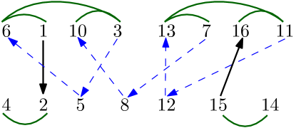
Figure 2: The green brackets indicate down-pairs. The lower sequence contains three solitaires, namely 5, 8, and 12. The solitaire $5$ is enclosed by the down-pair $(6,3)$ and hence we have the tentative edges $3\dashrightarrow 5\dashrightarrow 6$. The solitaire $8$ is enclosed by the down-pair $(10,7)$ and hence $7\dashrightarrow 8\dashrightarrow 10$. The solitaire 12 is enclosed by $(13,11)$ and hence $11\dashrightarrow 12\dashrightarrow 13$. We also have the strict edges $1\rightarrow 2$ and $15\rightarrow 16$. There are more edges not drawn here. The two sequence are not mergeable. Since we have the strict edge $1\rightarrow 2$, we cannot realize $5\dashrightarrow 6$. Thus we must realize $3\dashrightarrow 5$ and hence cannot realize $8\dashrightarrow 10$. Thus we must realize $7\dashrightarrow 8$ and hence cannot realize $12\dashrightarrow 13$. Thus we must realize $11\dashrightarrow 12$. This conflicts the strict edge $15\rightarrow 16$.
Without the element 14 in the lower sequence, the two sequences can be merged into $4,6,1,2,10,3,5,13,7,8,16,11,12,15$. Instead of the solid edge $15\rightarrow 16$, we have the tentative edges $11\dashrightarrow 15\dashrightarrow 16$. The former is realized.

2.3 Merging in linear time

We give a linear time implementation of the algorithm of Section 2.2, in particular, we show that there is no need to construct the precedence graph, but that the decisions of which first element to move to the output can be made locally after a small amount of precomputation. This is the content of Lemma 2.12. After the Lemma, we show how to compute the information required for the refined rules in linear time.

Lemma 2.12.

Let $c_{i}$ be the head of the $i$-th queue; here queue means the suffix of elements that are not dequeued yet.

1. If $c_{i}$ is smaller than all elements in the other queue, it is free.

2. If neither $c_{1}$ nor $c_{2}$ is a left element, the smaller of the two is free.

3. If a $c_{i}$ is a left element, it is blocked iff the other queue contains a smaller left element. If there is such a left element in the other queue, it is the leftmost left element.

   If there is no such left element in the other queue, $c_{i}$ is half-blocked iff the other queue contains a solitaire $s$ such that $c_{i}>s>r_{i}$, where $r_{i}$ is the first right element after $c_{i}$.

4. We now assume that at least one first element is a left element and that both queues contain an element smaller than the first element in the other queue.

   1. If both first elements are left elements, the larger is blocked and the smaller is non-blocked.

   2. Assume the first queue starts with a left element $\ell_{1}$ and the second queue starts with either a right element or a solitaire. Let $r_{1}$ be the first right element after $\ell_{1}$. Then $\ell_{1}>c_{2}>r_{1}$.

   3. If one first element is a left element and the other is a right element, the right element is blocked.

   4. If one first element is a left element and the other is a solitaire and a left element larger than the solitaire has already been dequeued, the solitaire is blocked.

   5. If one first element is a left element and the other is a solitaire and no left element larger than the solitaire was already dequeued, the solitaire is half-blocked and smaller than the left element.

5. The above covers all cases.

Proof 2.13.

1. All constraint edges between sequences go from smaller to larger element.

2. If $c_{i}$ is a right element or a solitaire, all elements after $c_{i}$ in the $i$-th queue are larger than $c_{i}$. Thus, if neither first element is a left element, the smaller first element is free.

3. A solid incoming edge into a left element can only come from a smaller left element. The leftmost left element is the smallest left element in the other queue.

   A tentative incoming edge can only come from a solitaire with $c_{i}>s>r_{i}$ where $r_{i}$ is a right element in $c_{i}$’s queue. If there is such an $r_{i}$, it is the first right element.

4. 1. We have the strict edge $\min(\ell_{1},\ell_{2})\rightarrow\max(\ell_{1},\ell_{2})$ and hence the larger is blocked. The smaller is either free or half-blocked.

   2. Assume the first queue starts with a left element $\ell_{1}$. There must be a right element $r_{1}$ after it in the first queue. $r_{1}$ is the smallest element in the first queue and hence $c_{2}>r_{1}$. If the first element in the second queue is either a solitaire or a right element, it is the smallest element in the second queue. Thus $\ell_{1}>c_{2}$.

   3. Assume $c_{1}$ is a left element and $c_{2}$ is a right element. Let $r_{1}$ be the first right element in the first queue. Then $r_{2}>r_{1}$ by the preceding item and hence we have a strict edge from $r_{1}$ to $r_{2}$ and hence $r_{2}$ is blocked.

   4. Assume the first queue starts with a left element. Then $\ell_{1}>s_{2}>r_{1}$, where $r_{1}$ is the first right element in the first queue. If a left element $\ell^{\prime}_{1}$ with $\ell^{\prime}_{1}>s_{2}$ was already dequeued, the tentative edge $s_{1}\dashrightarrow\ell^{\prime}_{1}$ was not realized and hence the tentative edge $r_{1}\dashrightarrow s_{1}$ became solid.

   5. Assume the first queue starts with a left element. Then $\ell_{1}>s_{2}>r_{1}$, where $r_{1}$ is the first right element in the first queue. All left elements already dequeued from the first queue are smaller than $s_{2}$ and hence all tentative edges $r\dashrightarrow s_{1}$ from a right element in the first queue into $s_{2}$ are still tentative. We also have the tentative edges $r_{1}\dashrightarrow s_{1}\dashrightarrow\ell_{1}$. Thus $s_{1}$ is half-blocked.

5. If neither first element is a left element, the smaller is free and moved to the output (item 2). If a first element is a left element, items 3 tells whether the element is free, half-blocked, or blocked. If both first elements are left elements, item 4a tells which one to move. If one first element is a left element, and the other is either a right element or a solitaire, items 4c, 4d, and 4f tell the status of the other element.

What is needed to implement the preceding Lemma?

• Each element needs to know its type: left or right element or solitaire.

• For each suffix of a queue, we need to know the smallest right element in the suffix, the smallest left element in the suffix, and the smallest solitaire in the suffix.

• The largest left element already dequeued.

Lemma 2.14.

If the information above is available, all decisions in Lemma 2.12 can be made in constant time. The above information can be precomputed in linear time.

Proof 2.15.

We go through the various items of Lemma 2.12 and argue that the decision can be made based on the information above. For the decisions in cases 1, 2, 3, 4a, 4b, 4c, and 4d, the information of the first two items suffices. For the case distinction 4e or 4f, one also needs the third item.

Item 3 needs an additional explanation. If $c_{i}$ is a left element and we have $c_{i}>s>r_{i}$ for some solitaire in the other queue and $r_{i}$ the first right element in $c_{i}$’s queue, $s$ is not necessarily the first solitaire in the other queue. However, if the first solitaire in the other queue is smaller than $c_{i}$ and $r_{i}$, then it is smaller than all elements in $c_{i}$’s queue. Thus the solitaire is free and it does not matter whether $c_{i}$ is free of half-blocked.

An element is a right element if there is a larger element to the left of it. We scan the sequence from left to right and maintain the maximum. Left elements are determined by a right to left scan. Elements that are neither left nor right are solitaires. For the second item, we do a right to left scan, and the third item is kept during the execution.

The algorithm above either produces an output of LDS two or stops because both first elements are blocked. Can we in the latter case at least produce an output of LDS three? Yes, we simply continue with the Smallest Element First strategy.

Theorem 2.16.

If both first elements are blocked, continuing with the Smallest Element First  strategy will produce an output of LDS three.

Proof 2.17.

It is clear that Smallest Element First runs to completion. So we only have to show that the output has LDS three. We first show that among two left elements, the smaller is always output before the larger. This is clear if they come from the same queue as the smaller precedes the larger. If they come from different queues and one of them is output before the algorithm blocks, this holds true, because we have a strict edge from the smaller to the larger. So assume that both are output by Smallest Element First. Let $\ell_{1}$ and $\ell_{2}$ be two left elements with, say, $\ell_{1}<\ell_{2}$, and assume that $\ell_{2}$ is output before $\ell_{1}$ by Smallest Element First. Consider the situation just before $\ell_{2}$ is output. All elements preceding $\ell_{1}$ in its queue are smaller than $\ell_{1}$ and hence Smallest Element First  will output them and $\ell_{1}$ before $\ell_{2}$.

So a decreasing sequence can involve at most one left element. It can also involve at most one solitaire. So, if it has length four, it must involve two right elements, one from each queue. One of them must come from the same queue as the solitaire. But this is impossible, because solitairs are larger than all preceding elements and smaller than all succeeding elements.

2.4 The limits of reducing LDS

The above algorithm can be used for the dequeuing step in algorithm that is supposed to reduce the LDS of a given sequence with an LDS of at most $4$. However, it is not straight forward to see whether we can always enque such a given sequence into two queues s.t. both queues contain mergable sequences. It turns out this is not the case – there exist sequences of LDS $L$, such that with $k$ queues it is impossible to reduce it to a value lower than $L-k+1$. We will first show this result for the case $k=2$ in order to make it easier to build an intuition for the proof. Afterwards, we present the general case. We begin with the following definition.

Definition 2.18.

Given a sequence $A$, we define $\Lambda_{k}(A)$ to be the lowest possible obtainable LDS of a sequence generated by enqueuing and dequeuing the sequence $A$ using $k$ parallel queues.

Let $L\in\mathbb{N}$. In this section, we prove that for each $L\in\mathbb{N}$, there is a sequence $A$ of LDS $L$ such that $\Lambda_{k}(A)\geq L-k+1$. The proof is constructive, and the length of the constructed sequence $A$ is $\Theta(L^{2k-1})$. Formally,

Theorem 2.19.

For every $L$ and $k$, there exists a sequence $A$ of LDS $L$ such that $\Lambda_{k}(A)\geq L-k+1$. The length of $A$ is $\Theta(L^{2k-1})$.

We first present a construction when $k=2$, and then extend it to any fixed $k$. We then show that the bound the length of the constructed sequence. Towards this, we briefly recall the definition of the direct and skew sum of permutations, that is required for our construction. Given two permutations $\pi$ and $\sigma$, and their respective permutation matrices $M_{\pi}$ and $M_{\sigma}$, the direct sum and skew sum of these two permutations, in terms of permutation matrices, take the form

$$M_{\pi}\oplus M_{\sigma} =\begin{bmatrix}M_{\pi}&0\\ 0&M_{\sigma}\end{bmatrix}\qquad\text{and} M_{\pi}\ominus M_{\sigma} =\begin{bmatrix}0&M_{\pi}\\ M_{\sigma}&0\end{bmatrix}\text{, respectively.}$$

Equivalently, we can define the direct sum of two permutations $\pi$ and $\sigma$ as

$$\pi\oplus\sigma=\pi\mathbin{\|}\sigma^{\prime},$$

where $\sigma^{\prime}$ is obtained from $\sigma$ by adding $|\pi|$ to all its elements, and the skew sum as

$$\pi\ominus\sigma=\pi^{\prime}\mathbin{\|}\sigma,$$

where $\pi^{\prime}$ is obtained from $\pi$ by adding $|\sigma|$ to all its elements.

2.4.1 Lower bound with $2$ queues

Here, we fix an integer $L\in\mathbb{N}$ as the LDS of the constructed sequence. We present a permutation $\pi$ with LDS $L$ such that any manner of enqueueing it into $k=2$ queues and then dequeueing it yields an outgoing permutation of LDS at least $L-1$. We prove this claim by induction on the value of the LDS.

The following two observations are crucial for the understanding of the lower bound with $2$ queues and with $k$ queues.

• Consider the direct sum $\pi\oplus\sigma$. In the resulting sequence, all the elements that originally belonged to $\pi$ are lower than those which originally belonged to $\sigma$. Furthermore, the LDS of $\pi\oplus\sigma$ is the maximum between the LDS of $\pi$ and the LDS of $\sigma$.

• Consider the skew sum $\pi\ominus\sigma$. In the resulting sequence, all the elements that originally belonged to $\pi$ are greater than those which originally belonged to $\sigma$. Furthermore, the LDS of $\pi\ominus\sigma$ is the sum of the LDS of $\pi$ and the LDS of $\sigma$.

Theorem 2.20.

For every $L\in\mathbb{N}$, there exists a permutation $\pi$ with LDS $L$, such that $\Lambda_{2}(\pi)\geq L-1$.

Proof 2.21.

We set the base case to be $L=3$. In this case $\pi=[3,2,1]$. It is easy to see that the LDS is $3$ and that with only two queues it’s not possible to obtain an output LDS lower than $2$. In other words it’s not possible to perfectly sort this sequence in ascending order.
To proceed with the inductive step, for each $L\in\mathbb{N}$ denote $A_{L}$ to be a specific permutation of LDS equals to $L$ such that $\Lambda_{2}(A_{L})\geq L-1$. A recursive formulation for $A_{L}$ is the following

$$A_{L+1}=(A_{L}\oplus\underbrace{D_{L}\oplus\dots\oplus D_{L}}_{L-1\text{ times}})\ominus[1]$$

Where $D_{L}$ denotes the decreasing sequence of length $L$, and the corresponding permutation matrix is simply the anti-diagonal matrix of size $L$. The permutation matrix of $A_{L}$ is of the form

$$A_{L+1}=\begin{bmatrix}0&A_{L}&0&0&\dots&0\\ 0&0&D_{L}&0&\dots&0\\ 0&0&0&D_{L}&\dots&0\\ \vdots&\vdots&\vdots&\vdots&\ddots&\vdots\\ 0&0&0&0&\dots&D_{L}\\ 1&0&0&0&\dots&0\end{bmatrix}\qquad$$

From Observation 2.4.1 it follows that $A_{L+1}$ is a permutation of LDS $L+1$. We prove that $\Lambda_{2}(A_{L+1})\geq L$. We refer to $B_{i}$ and $C_{i}$ as the subsequences of the $i$-th copy of $D_{L}$ which have been enqueued into the first and the second queue respectively, where $1\leq i\leq L-1$. In the same way, we call $X$ and $Y$ the sequences in the first and second queue dequeued from $A_{L}$. W.l.o.g. assume that the element $1$ is pushed in the first queue. This means that it is dequeued after $X$ and all the sequences $B_{i}$. We consider two following cases:

• The element $1$ is dequeued after the last element of $Y$: Since the elements of $X$ are in the same queue as the element $1$, the $1$ is also dequeued after the last element of $X$. Therefore, all the elements of $X$ and $Y$ will appear before the element $1$ in the final sequence. By the inductive hypothesis, merging the two sequences $X$ and $Y$ will create a decreasing sequence of length $L-1$. Since the element $1$ is dequeued afterwards, we obtain a decreasing sequence of length $L$.

• The element $1$ is dequeued before the last element of $Y$: Denote the LDS of the sequences $B_{1},B_{2},\dots,B_{L-1}$ as $\ell_{1},\dots,\ell_{L-1}$, respectively. If any $\ell_{i}\geq L-1$, when the element $1$ is appended at the end of the sequence, the sequence $B_{i}\cup\{1\}$ will have an LDS $\geq L$, trivially satisfying the claim of the theorem. Similarly, if $\ell_{i}=0$, the sequence $C_{i}=D_{L}$, which has the LDS $=L$. We can therefore assume that $1\leq\ell_{i}\leq L-2\>\>\forall i\in[L-1]$. By pigeonhole principle, there exists a pair $i,j$, with $i<j$, such that $\ell_{i}=\ell_{j}$. Notice that, by the construction of $A_{L+1}$, all the elements of $B_{j}$ are greater than all the elements of $C_{i}$. The element $1$ is dequeued before the last element of $Y$, hence it is dequeued before any sequence $C_{i}$. This means that all the sequences $B_{i}$ are dequeued before all the sequences $C_{i}$. Since $\ell_{i}=\ell_{j}$, it’s easy to see that the LDS given by the concatenation of $B_{j}$, having LDS of $\ell_{i}$, and $C_{i}$, having LDS of $L-\ell_{i}$, is equal to $L$, which proves the claim.

To analyze how quickly the size of $A_{L}$ grows, we can compute its length recursively. It is composed by the concatenation of $A_{L-1}$, with unknown length, and $L-2$ sequences $D_{L-1}$, with length $L-1$, and finally of the element $1$. Trivially, we obtain that $size(A_{L})=size(A_{L-1})+(L-2)\cdot(L-1)+1$, where $size(A_{3})=3$. One can easily check that the closed form is $size(A_{L})=\frac{L(L^{2}-3L+5)}{3}-2$.

2.5 Lower bound in the generalized case with $k$ queues

In this part, we present a permutation $\pi$ with LDS $L$ such that $\Lambda_{k}(\pi)\geq L-k+1$. The intuition is similar to the case where $k=2$. The primary difference is that for $k=2$ we had $L-1$ repetitions of $D_{L}$ in the construction of $A_{L}$. Instead of $L-1$ repetitions, we have $(L-k+1)(k-1)$ repetitions for a general $k$.

Definition 2.22.

Define a sequence of permutations $\{B_{L}^{k}\}_{L=1}^{\infty}$ by following rules:

• For any $L$, set $B_{L}^{1}$ to be a decreasing sequence of length $L$.

• For each $1\leq L\leq k+1$, set $B_{L}^{k}$ to be a decreasing sequence of length $L$.

• For every $L\geq k+2$, with $k\geq 2$, consider the following recursion for $B_{L+1}^{k}$:

  $$B_{L+1}^{k}=(B_{L}^{k}\oplus\underbrace{B_{L}^{k-1}\oplus\dots\oplus B_{L}^{k-1}}_{(L-k+1)(k-1)\text{ times}})\ominus[1].$$

Observe that, for $k=2$, the recursion above is the same as in previous subsection. Similarly to the case for $k=2$, one can easily show that the LDS of $B_{L}^{k}$ is exactly $L$. So it remains to prove that $\Lambda_{k}(B_{L}^{k})\geq L-k+1$ for all $L\geq k+1$. Note that for every $L\leq k$, it’s possible to yield a sorted sequence as the result. It is also easy to see that for $L=k+1$, the lowest obtainable LDS is $2=L-k+1$, because, by the pigeonhole principle, at least two elements will be enqueued on the same queue.
Before proceeding with the main Lemma, we first state and prove some lemmas that will turn useful later.

Definition 2.23.

Sequences $A^{\prime}$ and $A^{\prime\prime}$ are called a split of $A$ if $A^{\prime}$ and $A^{\prime\prime}$ are disjoint subsequences of $A$ and $A$ is an interleaving of $A^{\prime}$ and $A^{\prime\prime}$.

Lemma 2.24.

For any split $A$, $B$ of some sequence $C$, if $\Lambda_{s}(A)=\ell$ and $\Lambda_{s^{\prime}}(B)=t$, then $\Lambda_{s+s^{\prime}-1}(C)\leq\ell+t$.

Before proceeding with the proof we make some remarks and claims to make the proof more intuitive and easier to verify. Consider a sequence $D$ being completely enqueued and completely dequeued through $k$ queues, and resulting in a sequence $D^{\prime}$. Let’s denote the enqueuing protocol, that is, the policy used to enqueue $D$, $S_{e}$ and the dequeuing protocol $S_{d}$. We can encode $S_{e}$ into a string, where the $i$-th element is an integer, indicating the index of the queue where the $i$-th element of $D$ should be enqueued to. For example, the string {1, 3, 2} encodes a protocol that enqueues the first element into $Q_{1}$ the second element into $Q_{3}$ and the third element into $Q_{2}$. We can encode $S_{d}$ in the same way, but this time, each element indicates the index of the queue the $i$-th element of the resulting sequence should be dequeued from.

Claim 2.

The following two ways to execute the protocols are equivalent and they both result in the same sequence $D^{\prime}$.

• First enqueue all the elements of $D$ according to $S_{e}$ and afterwards dequeue them according to $S_{d}$.

• If the next element in $S_{d}$ is available in the respective queue, dequeue it, otherwise enqueue the next element according to $S_{e}$. Repeat until the starting sequence and all the queues are empty.

The first case coincides with the construction of $S_{e}$ and $S_{d}$. Therefore, it trivially leads to $D^{\prime}$. By executing the protocol $S_{e}$, we are iterating over its encoded string until we reach the end, and afterward we iterate over the string of $S_{d}$.

Assume the resulting sequence $D^{\prime\prime}$ of the second case is different, and that the first position where it differs is $i$. It means that the $i$-th element which gets dequeued is different in $D^{\prime}$ and $D^{\prime\prime}$. Since in both cases we used the same protocol $S_{d}$, the queue from which this element is dequeued is the same. Since we also execute the same enqueuing protocol $S_{e}$ as well, the relative ordering of the elements inside the same queues is preserved and cannot result in different elements at the same position.

Claim 3.

In the second case of Claim 2, at each step, there is always at least one queue that either is empty, or that has a single element which is dequeued as soon as it is enqueued.

If all the queues have at least one element which is not immediately dequeued, it means that at the head of all the queues there is an element, and that no one of them can be dequeued. By enqueuing more elements in the queues, the elements at the head of the queues don’t change and the dequeuing protocol is blocked and cannot be executed, which, by construction, is a contradiction. Notice that the queue is not necessarily the same all the time, however, the protocol can be modified to achieve this. We follow the same terminology of [17] and we denote this queue as express queue.

Claim 4.

It is always possible to modify the protocols $S_{e}$ and $S_{d}$ such that the result is the same and such that there is a fixed queue that is always either empty or with a single element that is immediately dequeued.

The only way the “temporary” express queue can change is that there is more than one empty queue which blocks the dequeuing protocol from being executed. For example, assume $Q_{1}$ is currently the express queue. Then, $Q_{2}$ gets emptied, and the dequeuing protocol requires an element from $Q_{2}$. If the enqueuing protocol enqueues elements in $Q_{1}$, the dequeuing protocol is still blocked by $Q_{2}$, which becomes the new express queue. In order to fix an express queue, the enqueuing and dequeuing protocol must be modified such that, whenever there is more than one empty queue, the last queue to receive an element from the enqueuing protocol is the desired express queue. By doing so, the fixed queue cannot be blocked by other empty queues, because it is the last one to stay empty. We proceed with the proof of Lemma 2.24.

Proof 2.25.

After enqueuing and dequeuing $A$ through $s$ queues we can obtain a sequence $A^{\prime}$ with LDS of $\ell$. Denote the protocol to get this result as $S^{\prime}$. Similarly, denote the protocol for $B$ that results in $B^{\prime}$ with LDS of $t$, as $S^{\prime\prime}$. Now modify $S^{\prime}$ and $S^{\prime\prime}$ according to Claim 4 such that they both have an express queue. W.l.o.g. we can assume that the express queue is the first queue in both cases. Now we show how to enqueue-dequeue $C$ through $s+s^{\prime}-1$ queues in order to get an LDS of $\ell+t$.
Enqueue the $i$-th element $e$ of $C$ as follows:

• If $e$ is an element of $A$, enqueue it according to $S^{\prime}_{e}$;

• If $e$ is an element of $B$, let $q\in[s^{\prime}]$ be the index of the queue where it is supposed to be enqueued according to $S^{\prime\prime}_{e}$:

  • If $q=1$, i.e., the express queue, enqueue $e$ in the first queue;

  • Otherwise, enqueue $e$ in the queue with index $q+s-1$ and modify the dequeuing protocol $S^{\prime\prime}_{d}$ accordingly.

We can now dequeue the elements of $C$ according to $S^{\prime}_{d}$ and $S^{\prime\prime}_{d}$ where the origin of the head of the first queue determines which of the two is currently active. We thereby obtain a sequence $C^{\prime}$ with an LDS that is at most the sum of the LDS of $A^{\prime}$ and $B^{\prime}$, i.e., $\ell+t$.

Lemma 2.26.

For any split $A^{\prime}$, $A^{\prime\prime}$ of some sequence $A$, if $\Lambda_{k}(A)=L$ and $\Lambda_{s}(A^{\prime})=\ell$, with $s<k$, then $\Lambda_{k-s+1}(A^{\prime\prime})\geq L-\ell$.

Proof 2.27.

For sake of contradiction, assume $t:=\Lambda_{k-s+1}(A^{\prime\prime})<L-\ell$. By Lemma 2.24, we can enqueue-dequeue $A$ with $k=s+k-s+1-1$ queues, such that the LDS of the result is at most $\ell+t<\ell+L-\ell=L$, a contradiction to $\Lambda_{k}(A)=L$. Therefore, $t\geq L-\ell$.

This Lemma is crucial for the proof and it encloses the main idea. The intuition is that we are going to split a sequence $B_{L}^{k-1}$ in two parts. The first part is sorted with $s$ queues and leads to an LDS of $\ell$, the second part is going to be sorted with $k-s$ queues and leads to an LDS of $L-k+2-\ell$, because we will assume by induction that $\Lambda_{k-1}(B_{L}^{k-1})=L-k+2$. The fact that if we split it in two parts, the sum of the LDSs, $\ell$ and $L-k+2-\ell$, is at least the original LDS, i.e., $L-k+2$, will be the main point. Now we can state and prove the main Theorem.

Theorem 2.28.

$\Lambda_{k}(B_{L}^{k})\geq L-k+1$ for all $k\geq 1$ and for all $L\geq k+1$.

Proof 2.29.

The proof follows by double induction on $L$ and $k$. First we set the base case for $k=1$ and we prove the claim for every $L$. Recall that in this case $B_{L}^{1}$ is a decreasing sequence of length $L$. Obviously with a single queue the sequence does not change and the resulting sequence has an LDS of $L=L-k+1$.

Now we set the base case for $L=k+1$ and we prove the claim for every $k$. We have already argued that, by the pigeonhole principle, the lowest possible obtainable LDS for $B_{k+1}^{k}$ with $k$ queues is $2=L-k+1$.

Now we proceed with the induction step and we set $k\geq 2$ and $L\geq k+2$. We want to prove that $\Lambda_{k}(B_{L+1}^{k})\geq L-k+2$, and we will make the following two assumptions by induction:

• $\Lambda_{k}(B_{L}^{k})\geq L-k+1$;

• $\Lambda_{k-1}(B_{L}^{k-1})\geq L-(k-1)+1=L-k+2$.

Let’s denote $P_{i}^{j}$ to be elements of the $i^{th}$ copy of $B_{L}^{k-1}$ which are enqueued to the $j^{th}$ queue, with $1\leq i\leq(L-k+1)(k-1)$. Similarly, let’s also denote $P_{0}^{j}$ to be the elements of $B_{L}^{k}$. For example, in the proof of Theorem 2.20, $C_{i}$, which was in the second queue, would be $P_{i}^{2}$, and $X$, in the first queue, would be $P_{0}^{1}$ in this case. W.L.O.G. assume that the element $1$ is enqueued in the first queue.
Before proceeding, we prove another intermediate claim. For the sequel, we split the $(k-1)(L-k+1)$ occurrences of $B_{L}^{k-1}$ into $k-1$ disjoint blocks of $L-k+1$ consecutive occurrences each. For a block $Q$, we use $Q^{j}$ to denote the elements that are enqueued into the $j$-th queue.

Claim 5.

Given the construction of $B_{L+1}^{k}$, at least one of the following is true:

1. All the sequences $P_{0}^{j}$ are dequeued before the element $1$;

2. There is a block $Q$ such that each $Q^{j}$, $j\in[k]$, is either completely dequeued before 1 or completely dequeued after 1. Moreover, at least one $Q^{j}$ is completely dequeued before $1$ and one is completely dequeued after $1$.

Assume we are not in case 1, i.e., $1$ is dequeued before the last element of some $P_{0}^{p}$. Then $p>1$, since $1$ is dequeued after all elements in the first queue. Say that a queue $j$ kills a block $Q$ if $1$ is dequeued after the first element of $Q^{j}$ and before the last of $Q^{j}$. Then queues $1$ and $p$ kill no block and any other queue can kill at most one block. So one block is not killed as we have $k-1$ blocks but only $k-2$ queues that can kill a block.

We consider the two cases separately:

1. Recall that the sequences $P_{0}^{j}$ are the result of enqueuing the elements of $B_{L}^{k}$. By the inductive hypothesis $\Lambda_{k}(B_{L}^{k})\geq L-k+1$. By assumption $1$ is output after all elements of $B_{L}^{k}$ and hence an LDS of at least $L-k+2$ will result.

2. We have a block $Q$ of $L-k+1$ occurrences of $B_{L}^{k-1}$ such that $1$ is either dequeued before or after all items of each $Q^{j}$. Also $1$ is dequeued after all elements in $Q^{1}$ and before all elements of $Q^{p}$ for some $p>1$.

   We may assume that there is an $s$ with $2\leq s\leq k-1$ such that the $Q^{j}$ with $1\leq j\leq s$ are dequeued before 1 and the $Q^{j}$ with $s+1\leq j\leq k$ are dequeued after 1.

   For $i\in[L-k+1]$, let $P_{i}$ be the $i$-th occurrence of $B_{L}^{k-1}$ in $Q$ and let $P^{j}_{i}$ be elements of the $i$-th occurrence which are enqueued in queue $j$. If some $P^{j}_{i}$ is empty, $P_{i}$ is enqueued into fewer than $k$ queues and hence the result has an LDS of at least $L-k+2$ by induction hypothesis.

   We use $P_{i}^{j\in[s]}$ to denote the ensemble $P_{i}^{j}$, $j\in[s]$. Let $\ell_{i}$ be the minimum LDS that any dequeuing of $P_{i}^{j\in[s]}$ can achieve. Since $P_{i}^{j}$ is non-empty for all $j$, $\ell_{i}\geq 1$.

   Assume next that there is an $\ell_{i}\geq L-k+1$. Then together with the element 1 we obtain a decreasing subsequence of length $L-k+2$.

   So we are left with the case that $1\leq\ell_{i}\leq L-k$ for all $\ell$. Therefore there must be indices $u$ and $v$ such that $1\leq u<v\leq L-k+1$ and $\ell_{u}=\ell_{v}$. Note that all elements in $P_{v}$ are greater than all elements in $P_{u}$. Note also that we are not claiming that $P_{u}$ and $P_{v}$ are enqueued in the same way. We are only claiming that both enqueuings give the same LDS.

   We next apply Lemma 2.26 to $A=P_{u}$, $A^{\prime}$ the subsequence of $P_{u}$ that is enqueued into the first $s$ queues and $A^{\prime\prime}$ the subsequence that is enqueued into the other $k-s$ queues. Since $\Lambda_{k-1}(B_{L}^{k-1})=L-k+2$ and $\Lambda_{s}(A^{\prime})=\ell_{u}$, we have $\Lambda_{k-s}(A^{\prime\prime})=\Lambda_{k-1-s+1}(A^{\prime\prime})\geq L-k+2-\ell_{u}$.

   Now we are done. In the output, we have a decreasing subsequence of length $\ell_{v}$ resulting from the dequeuing of $P_{v}^{j\in[s]}$ followed by a decreasing sequence of length $L-k+2-\ell_{v}=L-k+2-\ell_{u}$ resulting from the dequeuing of the $P_{u}^{j}$, $s<j\leq k$. Note that all elements in the former sequence are larger that all elements in the latter sequence. Hence an LDS of $L-k+2$ results.

This completes the proof of this theorem.

2.5.1 Growth of the sequence

We now show that the length of the sequence $B_{L}^{k}$ is $\Theta(L^{2k-1})$. Denote by $S_{L}^{k}$ the length of the sequence $B_{L}^{k}$. For the case $k=2$ we have seen that $S_{L}^{2}=\frac{L(L^{2}-3L+5)}{3}-2\in\Theta(L^{3})$. For the general case, given the construction of $B_{L}^{k}$, $S_{L}^{k}$ will be of the following form:

$$S_{L}^{k}=S_{L-1}^{k}+(L-k)(k-1)S_{L-1}^{k-1}+1.$$

By expanding the recursive formula only on the first term, where only one index is decremented, we can reduce it to

$$S_{L}^{k}=L+(k-1)\sum_{i=2}^{L-k}iS_{k-1+i}^{k-1}=L-(k-1)k+(k-1)\sum_{i=k}^{L-1}(i-k+1)S_{i}^{k-1}$$

where we used that $S_{k+1}^{k}=k+1$ and that $S_{k}^{k-1}=k$. Using this rewriting of the formula, we can prove the claim by induction.
The base case $S_{L}^{1}$ is trivial, as $S_{L}^{1}=L$. We now assume that $S_{L}^{k-1}\in\Theta(L^{2k-3})$. The term that will result in the highest degree is $\sum_{i=k}^{L-1}iS_{i}^{k-1}$. In particular, $iS_{i}^{k-1}\in\Theta(i^{2k-2})$, by the inductive hypothesis. Since we sum the indices $i$ up to $L$, we get a polynomial one degree higher. Hence $S_{L}^{k}\in\Theta(L^{2k-1})$.

3 Minimizing Downsteps

With the results of the previous section, it is not clear whether having several multilane buffers in a row is better than having all lanes in parallel in a single buffer. However, with the measure of disorder that we consider in this section, namely the number of downsteps, we will see that a logarithmic number of multilane buffers in a row suffice to sort a sequence perfectly. Moreover, we present an optimal algorithm $\sf{Alg}_{\mathrm{DS}}$ for minimizing the number of downsteps in a sequence using $k$ queues. This algorithm runs in time $O(n\log k)$, where $n$ is length of the sequence. Further, this algorithm is online.

The algorithm is as follows: Recall that we have $k$ queues and our input is a sequence of length $n$. For simplicity we assume that all numbers in the input are non-negative. We define the enqueuing and dequeuing strategy of our algorithm $\sf{Alg}_{\mathrm{DS}}$ and then prove its optimality.

Enqueuing:

The queues are numbered $0$ to $k-1$. We denote the last element in queue $i$ by $\ell_{i}$. Initially, when all queues are empty, $\ell_{i}$ has the fictitious value $-i-1$. One of the queues is the base queue; we use $b\in[k-1]$ to denote the base queue. Initially, $b=0$. We maintain the following invariant at all times:

$$\ell_{b}>\ell_{b+1}>\ldots>\ell_{b+k-1}.$$

Indices are to be read modulo $k$. Note that the fictitious values are chosen such that the invariant holds initially.

Assume now that element $e$ is to be enqueued. Let $i\in\{0,1,\ldots,k-1\}$ be minimal (if any) such that $e>\ell_{b+i}$. If $i$ exists, either $i=0$ and $e>\ell_{b}$ or $i>0$ and $\ell_{b+i-1}>e>\ell_{b+i}$.

• If $i$ exists, we append $e$ to queue $b+i$. This does not create a down-step and maintains the invariant.

• If $i$ does not exist, i.e., $\ell_{b+k-1}>e$, we append $e$ to queue $b$ and increase $b$ by 1. This creates a down-step in queue $b$. The invariant is maintained.

A run is an increasing sequence. At the end of the enqueuing all queues contain an equal number of runs up to one. Note that the down-steps are generated in round-robin fashion. The first down-step is created in queue $0$, the second in queue $1$, and so on. The number of runs in a queue is one more than the number of down-steps in the queue.

The enqueuing strategy is inspired by Patience Sort [1]. Patience Sort sorts a sequence of numbers using a minimum number of queues. It is as above with one difference: if $e$ cannot be appended to an existing run, then it opens up a new queue.

Dequeuing:

We first merge the first runs in all queues into a single run, then merge the second runs in all queues, and so on. So the number of runs in the output sequence is the maximum number of runs in any of the queues.

It is clear that the algorithm can be made to run in time $O(n\log k)$. We keep the values $\ell_{i}$ in an array $A$ of size $k$. When an element $e$ is to be enqueued, we perform binary search on the sorted array $A[b..b+k-1]$; again indices are to be read modulo $k$.

Theorem 3.1.

Algorithm $\sf{Alg}_{\mathrm{DS}}$ constructs an output sequence with a minimum number of down-steps. It is an on-line algorithm and can be implemented to run in time $O(n\log k)$. If an online algorithm $A$ deviates from $\sf{Alg}_{\mathrm{DS}}$, the input sequence can be extended such that $A$ does worse than $\sf{Alg}_{\mathrm{DS}}$.

We give three quite different proofs for the first claim of the theorem in Sections 3.1, 3.2, and 3.4 respectively. The first proof is the shortest, but also the least informative. It shows that the execution of any algorithm can be transformed into an execution of $\sf{Alg}_{\mathrm{DS}}$ without increasing cost. The second proof uses a potential argument and establishes that $\sf{Alg}_{\mathrm{DS}}$ is the unique optimal online algorithm. The third proof constructs witnesses for down-steps. In Section 3.3 we characterize the runs generated by the algorithm in the different queues without reference to the algorithm.

3.1 Transformation to $\sf{Alg}_{\mathrm{DS}}$

Let $A$ be any algorithm. We will show that the queue contents constructed by $A$ can be transformed into the contents constructed by $\sf{Alg}_{\mathrm{DS}}$ without increasing cost.

Let $t$ be minimal such that $A$ and $\sf{Alg}_{\mathrm{DS}}$ differ, i.e, $A$ enqueues $e=e_{t}$ into queue $i$ and $\sf{Alg}_{\mathrm{DS}}$ enqueues $e$ into queue $j$ with $i$ different from $j$. We concentrate on the $i$-th and the $j$-th queue. Let $a_{i}$ and $a_{j}$ be the contents of these queues just before enqueuing $e_{t}$ and let $s_{i}$ and $s_{j}$ be their continuations by $A$. $s_{i}$ starts with $e$. We swap $s_{i}$ and $s_{j}$, i.e, the contents of the $i$-th queue become $a_{i}s_{j}$ and the contents of the $j$-queue becomes $a_{j}s_{i}$. The number of down-steps stays the same except maybe for the down-steps at the borders between the $a$-parts and the $s$-parts.

We use $\ell(a_{i})$, $\ell(a_{j})$, $f(s_{i})$, and $f(s_{j})$ to denote the last and first elements of $a_{i}$, $a_{j}$, $s_{i}$ and $s_{j}$, respectively. We have $e=f(s_{i})$. We need to show that the number of down-steps in the pairs $(\ell(a_{j}),f(s_{i}))$ and $(\ell(a_{i}),f(s_{j}))$ is no larger than in the pairs $(\ell(a_{i}),f(s_{i}))$ and $(\ell(a_{j}),f(s_{j}))$.

We distinguish cases according to the action of $\sf{Alg}_{\mathrm{DS}}$. If $e$ is smaller than the last elements of all existing parts, $\sf{Alg}_{\mathrm{DS}}$ incurs a down-step and adds $e$ to the queue with largest last element. Otherwise, $\sf{Alg}_{\mathrm{DS}}$ appends $e$ to the queue whose last element is largest among the last elements smaller than $e$.

$e$ is smaller than all last elements:

Then all $k$ queues have a proper last element since $e$ is a non-negative number and fictitious last elements are negative. Thus $\ell(a_{j})>\ell(a_{i})>e$ where the first inequality follows from $i\not=j$ and the fact that the $j$-th queue has the largest last element and the second inequality holds because $e$ is smaller than all last elements. Thus we have a down-step in $a_{i}s_{i}$ and in $a_{j}s_{i}$. Let $e^{\prime}=f(s_{j})$. If we have no down-step in $a_{j}s_{j}$, then we have no down-step in $a_{i}s_{j}$ and hence the swap does does not increase the cost. If we have a down-step in $a_{j}s_{j}$, then $A$ incurred two down-steps before the swap and hence the swap cannot increase the cost. The swap decreases the number of down-steps if $\ell(a_{j})>e^{\prime}>\ell(a_{i})$.

$e$ is larger than some last element:

We have $\ell(a_{j})<e=f(s_{i})$, because $\sf{Alg}_{\mathrm{DS}}$ enqueues after the largest last element that is smaller than $e$. Thus, we have no down-step at the border from $a_{j}$ to $s_{i}$ and hence $A$ incurs at most one down-step after the swap. So, we only need to show that if the number of down-steps at the borders is zero before the swap then it is zero after the swap.

Assume the number is zero before the swap. Then $\ell(a_{i})<e=f(s_{i})$ and $\ell(a_{j})<f(s_{j})$. Also $\ell(a_{i})<\ell(a_{j})<e$, since $\sf{Alg}_{\mathrm{DS}}$ enqueus $e$ into the queue with largest last element smaller than $e$. Thus $\ell(a_{i})<f(s_{j})$ and $\ell(a_{j})<f(s_{i})$ and no down-step will be introduced by the swap.

We summarize:

Theorem 3.2.

No algorithm creates a smaller total number of down-steps over all queues than algorithm $\sf{Alg}_{\mathrm{DS}}$. Algorithm $\sf{Alg}_{\mathrm{DS}}$ generates an output with a minimal number of down-steps.

Proof 3.3.

We have shown how to convert the enqueuing of any algorithm into the enqueuing of $\sf{Alg}_{\mathrm{DS}}$ without increasing the total number of down-steps. $\sf{Alg}_{\mathrm{DS}}$ generates the same number of down-steps up to one in all queues and the number of down-steps in the output is equal to the maximum number of down-steps in any queue. Thus, every algorithm must generate at least as many down-steps in the output as $\sf{Alg}_{\mathrm{DS}}$.

3.2 A Potential Function Argument

We will use a potential function argument to show that no algorithm can create fewer down-steps than $\sf{Alg}_{\mathrm{DS}}$. We will also show that $\sf{Alg}_{\mathrm{DS}}$ is the unique optimal on-line algorithm. Let $A$ be any other algorithm. Let $a_{0}$ to $a_{k-1}$ be the last elements in the queues of algorithm $A$ and let $\ell_{b}>\ell_{b+1}>\ldots>\ell_{b+k-1}$ be the last elements in the queues of $\sf{Alg}_{\mathrm{DS}}$; $b$ is the base queue. Let $d_{A}$ be the number of down-steps created by $A$ and let $d_{O}$ be the number of down-steps created by $\sf{Alg}_{\mathrm{DS}}$. As the elements are added to queues by both algorithms, we maintain a bijection $\pi:\{0,\ldots,k-1\}\rightarrow\{0,\ldots,k-1\}$ and call an index $i$ good if $a_{\pi(i)}\geq\ell_{i}$. Otherwise, the index is bad. We show that the following invariant is maintained:

$$d_{A}-d_{O}+\max_{\pi}|\{i:a_{\pi(i)}\geq\ell_{i}\}|\geq k.$$

The invariant holds initially, since all indices are good (we initialize all $\ell_{i}$ and $a_{i}$ with fictious elements $-(i+1)$) and $d_{A}=d_{O}=0$. We use $d$ to denote $d_{A}-d_{O}$.

Assume now we enqueue an element $e$. We may also assume that $b=0$; otherwise renumber the queues of $\sf{Alg}_{\mathrm{DS}}$. We may assume that $\pi$ is the identity; otherwise renumber the queues of $A$. Let $a^{\prime}_{0},a^{\prime}_{1},\ldots,a^{\prime}_{k-1}$ and $\ell^{\prime}_{0},\ell^{\prime}_{1},\ldots,\ell^{\prime}_{k-1}$ denote the last elements of the queues of $A$ and $\sf{Alg}_{\mathrm{DS}}$, respectively, after adding $e$. Further, let $\pi^{\prime}$ denote the bijection after adding $e$.

Case, $e<\ell_{k-1}$:

Then $\sf{Alg}_{\mathrm{DS}}$ enqueues $e$ into queue 0 and $\ell^{\prime}_{0}=e$. Algorithm $A$ adds $e$ to queue $j$; note that $j=0$ is possible. Then $a^{\prime}_{j}=e$. We modify $\pi$ to $\pi^{\prime}$ by letting $0$ map to $j$ and $j$ map to $0$ (if $j=0$, we do not modify $\pi$).

$\sf{Alg}_{\mathrm{DS}}$ incurs a down-step and $d_{O}$ increases by $1$. Further the index $0$ is a good index after adding $e$, since $a^{\prime}_{j}=e=\ell^{\prime}_{0}$. Note that if $j$ was a good index, i.e., $a_{j}\geq\ell_{j}$, algorithm $A$ also incurs an down-step since $a_{j}\geq\ell_{j}\geq\ell_{k-1}>e$.

Observe that, if $j=0$ and $0$ was a good index before the addition, the invariant is maintained since both algorithms incur a down-step and $0$ stays a good index. Otherwise if $j=0$ and $0$ was a bad index before the addition, then the number of good indices is increased by one and $d$ decreases by at most one. The invariant is maintained when $j=0$.

So assume $j\not=0$. If neither $0$ nor $j$ was a good index before, the invariant is maintained since $d$ decreases by at most one and the number of good indices increases by at least one.

Assume next that exactly one of the indices was good: If $0$ was good and $j$ was not, $a_{0}\geq\ell_{0}$ and $a_{j}<\ell_{j}$ and hence $a^{\prime}_{\pi^{\prime}(j)}=a^{\prime}_{0}=a_{0}\geq\ell_{0}>\ell_{j}$ and $j$ is good after the addition. So the invariant is maintained since the number of good indices increases and $d$ decreases by at most one. Else if $j$ was good and $0$ was not, $a_{j}\geq\ell_{j}$ and hence $A$ also incurs a down-step. Thus $d$ does not change and the number of good indices does not increase. In either case, the invariant is maintained.

Assume finally that both indices were good. Then $a_{0}\geq\ell_{0}$ and $a_{j}\geq\ell_{j}$ before the addition of $e$. Then $j$ is good afterwards and $A$ incurs a down-step. So the number of good indices and $d$ do not change and the invariant is maintained.

Case, $e\geq\ell_{k-1}$:

Let $i$ be minimal such that $e\geq\ell_{i}$. Then either $i=0$ or $e<\ell_{i-1}$. Algorithm $\sf{Alg}_{\mathrm{DS}}$ adds $e$ to the $i$-th queue and algorithm $A$ adds $e$ to the $j$-th queue; $j=i$ is possible. Then $\ell^{\prime}_{i}=e=a^{\prime}_{j}$. Algorithm $\sf{Alg}_{\mathrm{DS}}$ does not incur a down-step and hence $d$ does not decrease. We change $\pi$ to let $i$ map to $j$ and $j$ map to $i$. If $i=j$, we do not modify $\pi$. Then $i$ is a good index after the addition of $e$. So the invariant is maintained if at most one of the indices $i$ and $j$ were good before the addition of $e$. Note that this includes the case of $i=j$.

So assume $i\not=j$ and $i$ and $j$ are good before the addition of $e$. Then $a_{i}\geq\ell_{i}$ and $a_{j}\geq\ell_{j}$. If $i<j$, then $a_{i}\geq\ell_{i}>\ell_{j}$ and hence $j$ is good after the addition of $j$. Thus the invariant is maintained. If $j<i$, then $a_{j}\geq\ell_{j}\geq\ell_{i-1}>e$ and hence $A$ incurs a down-step. So the number of good indices decreases by at most one and $d$ increases by one and hence the invariant is maintained.

Theorem 3.4.

No algorithm creates a smaller total number of down-steps over all queues than algorithm $\sf{Alg}_{\mathrm{DS}}$. Algorithm $\sf{Alg}_{\mathrm{DS}}$ generates an output with a minimal number of down-steps.

Proof 3.5.

By the invariant

$$d_{A}-d_{O}\geq k-\text{number of good indices}\geq 0,$$

and hence $d_{A}\geq d_{O}$. This proves the first part. For the second part, we observe that the number of down-steps in different queues differs by at most one and hence the number of down-steps in the output sequence created by $\sf{Alg}_{\mathrm{DS}}$ is at most $\left\lceil{d_{O}/k}\right\rceil$. Algorithm $A$ must create at least $\left\lceil{d_{A}/k}\right\rceil$ down-steps in one of the queues and hence the output.

We will next show that $\sf{Alg}_{\mathrm{DS}}$ is the unique optimal online algorithm. Recall that in an online algorithm the input is presented as a sequence $e_{1},e_{2}.\ldots,e_{j},\ldots$ and we have to pick a queue for element $e_{j}$ based on the current state of the queues and $e_{j}$. The processing of $e_{j}$ is independent of all the elements that follow it in the sequence.

Theorem 3.6.

$\sf{Alg}_{\mathrm{DS}}$ is the unique optimal online algorithm.

Proof 3.7.

Consider any other online algorithm $A$. Let $e_{1},e_{2},\ldots,e_{j},\ldots$ be the input sequence. When an element $e_{j}$ is to be enqueued an online algorithm chooses the queue based on the value of $e_{j}$ and the current contents of the queues, but independent of the continuation $e_{j+1},\ldots$. Assume now that $A$ is not identical to $\sf{Alg}_{\mathrm{DS}}$. Then there is an input sequence $e_{1},e_{2},\ldots,e_{j}$ such that $A$ and $\sf{Alg}_{\mathrm{DS}}$ act the same up to element $e_{j-1}$ but choose different queues for $e_{j}$. We will show that there is a continuation $e_{j+1},\ldots$ that forces $A$ to incur more down-steps than $\sf{Alg}_{\mathrm{DS}}$.

Let us first assume that all queues are in use when $e$ in enqueued. We may assume $b=0$. So $\ell_{0}>\ell_{1}>\ldots>\ell_{k-1}$ and these are also the tails of the queues for algorithm $A$. An element $e$ arrives.

Assume first that there is an $i$ such that $i=0$ and $e>\ell_{1}$ or $\ell_{i-1}>e>\ell_{i}$. Algorithm $\sf{Alg}_{\mathrm{DS}}$ adds $e$ to the $i$-th queue and algorithm $A$ adds $e$ to the $j$-th queue with $j\not=i$.

If $j<i$, $A$ incurs a down-step and we have an input sequence on which $A$ does worse.

If $j>i$, we have to work harder. The final elements of the queues are now:

algorithm $$\sf{Alg}_{\mathrm{DS}} \ell_{0}>\ldots>\ell_{i-1}>e>\ell_{i+1}>\ldots>\ell_{j-1}>\ell_{j}>\ell_{j+1}\ldots>\ell_{k-1}$$

algorithm A $$\ell_{0}>\ldots>\ell_{i-1}>e>\ell_{i}>\ell_{i+1}>\ldots>\ell_{j-1}>\ell_{j+1}>\ldots>\ell_{k-1}$$

We now insert $k-1-i$ elements that algorithm $\sf{Alg}_{\mathrm{DS}}$ can insert without incurring a down-step but A cannot. More precisely, we insert the decreasing sequence $\ell_{i+1}+\epsilon$, …, $\ell_{j}+\epsilon$, …$\ell_{k-1}+\epsilon$, where $\epsilon$ is an infinitesimal. Algorithm $\sf{Alg}_{\mathrm{DS}}$ can insert these elements into queues $i+1$ to $k$ without incurring a down-step. Algorithm A either has to put two of these elements in the same queue or one element in one of the first $i+1$ queues. In either case, it incurs a down-step.

We come to the case $e<\ell_{k}$. Algorithm $\sf{Alg}_{\mathrm{DS}}$ puts $e$ into queue 0, algorithm A puts $e$ into queue $j>0$. The final elements of the queues are now:

algorithm $$\sf{Alg}_{\mathrm{DS}} \ell_{1}>\ell_{2}>\ldots>\ell_{j-1}>\ell_{j}>\ell_{j+1}\ldots>\ell_{k-1}>e$$

algorithm A $$\ell_{0}>\ldots>\ell_{j-1}>\ell_{j+1}>\ldots>\ell_{k-1}>e$$

We next insert $\ell_{j}+\epsilon$, $\ell_{j+1}+\epsilon$, …, $\ell_{k-1}+\epsilon$. Algorithm $\sf{Alg}_{\mathrm{DS}}$ inserts these elements without incurring a down-step, but algorithm A must incur an down-step. The argument is as above.

We have now handled the situation when $A$ differs from $O$ after both algorithms fill all queues. We next deal with the situation where only $h<k$ queues are used and we have $\ell_{0}>\ldots>\ell_{h-1}$. An element $e$ is added. If $e>\ell_{h-1}$, we argue as above. If $e<\ell_{h-1}$ and A does not open a new queue, it incurs an down-step. If A opens a new queue, it does the same as $\sf{Alg}_{\mathrm{DS}}$.

3.3 Sequence Decomposition

In this section, we characterize the set of runs determined by algorithm $\sf{Alg}_{\mathrm{DS}}$.

Let $I_{0}$ be the input sequence. We will decompose $I_{0}$ into runs $s_{0}$, $s_{1}$, …and simultaneously construct modified input sequences $I_{1}$, $I_{2}$, …. The run $s_{i}$ is a run in $I_{i}$ and $I_{i+1}$ is obtained from $I_{i}$ by deleting the elements in $s_{i}$.

Assume $I_{j}$ is already defined. Let $f_{j}$ be the leftmost element in $I_{j}$ (if any) in which a decreasing sequence of length $k+1$ ends. If there is no such element, let $f_{j}$ be a fictitious element after the end of $I_{j}$. Let $s_{j}$ be leftmost increasing subsequence of the prefix $I_{j}[\text{up-to }f_{j}]$ of $I_{j}$ ending just before $f_{j}$, i.e., $s_{j}$ starts with the first element of $I_{j}$ and is then always extended by the first element that is larger than its last element.

Theorem 3.8.

Algorithm $\sf{Alg}_{\mathrm{DS}}$ constructs runs $s_{i}$, $s_{i+k}$, $s_{i+2k},\dots$ in queue $i$, $0\leq i<k$. Exactly the non-fictitious $f_{j}$ create down-steps.

Proof 3.9.

Let the rank of an element be the length of the longest decreasing subsequence ending in the element. Consider the execution of $\sf{Alg}_{\mathrm{DS}}$ on $I_{j}$ starting with empty queues and base queue $b$. Just before $f_{j}$ is enqueued, the elements of rank $i$, $0\leq i<k$, preceding $f_{j}$ in $I_{j}$ form the run in queue $q_{b+i}$. In particular, queue $q_{b}$ contains exactly the elements in $s_{j}$. When $f_{j}$ is enqueued into queue $b$, $b+1$ becomes the base queue and the contents of the queues $b+1$, …$b$ are now the elements of rank $0$, $1$, …$k-1$ in $I_{j+1}[\text{up-to and including }f_{j}]$.

3.4 Witnesses and Forced Down-steps

We associate witnesses with algorithm $\sf{Alg}_{\mathrm{DS}}$ that explain why elements were put into particular queues. Assume $e$ is the next element to be enqueued, $b$ is the base queue, and $\ell_{b}>\ell_{b+1}>\ldots>\ell_{b+k-1}$. Indices are to be read modulo $k$ and queues are indexed $0$ to $k-1$.

Initially $b=0$. We also set $j$ to zero. $b=j\bmod k$ will be an invariant. When an element is added to a queue which is not the base queue, we let it point to the last element in the preceding queue. In this way, if an element is added to a queue $b+j$, the pointer sequence has length (number of edges) at least $j$. Pointer sequences end in elements that were inserted into the current base queue.

We also construct a sequence $f_{0}$, $f_{1}$, $f_{2}$, …. They are the first elements of runs in each of the queues except for the first run in each queue. So for any $i\in[1,k-1]$ and any $j\geq 0$, $f_{jk+i}$ is the first element of run $j+1$ in queue $i$; runs are numbered starting at zero.

Recall the enqueuing algorithm. Let $e$ be the element to be enqueued. Let $i$ be minimal (if any) such that $e>\ell_{b+i}$.

• If $i$ exists, we append $e$ to $q_{b+i}$ and if $i>0$ we, in addition, let $e$ point to the last element of $q_{b+i-1}$.

• If $i$ does not exists, i.e., $e<\ell_{b+k-1}$, $e$ starts a new run in $q_{b}$. We append $e$ to $q_{b}$. This creates a down-step. We let $e$ point to the last element of $\ell_{b+k-1}$. Also $e$ becomes $f_{j}$ and we increment $b$ and $j$.

Enqueuing $f_{j}$ makes queue $j+1\bmod k$ the base queue.

Consider the first run in queue 1. The elements that were enqueued before $f_{0}$ have a pointer to queue 0, the elements that were enqueued after $f_{0}$ do not have a pointer to queue 0. Similarly for queue 2. The elements that were enqueued before $f_{1}$ have a pointer to queue 1, the elements that were enqueued after $f_{1}$ do not have a pointer to queue 1. Consider the second run in queue 2. The elements that were enqueued before $f_{k}$ have a pointer to queue 0, the elements that were enqueued after $f_{k}$ do not have a pointer to queue 0.

Theorem 3.10.

Let $f_{0}$ to $f_{t-1}$ be the non-fictitious $f$’s in our input sequence. Any algorithm must have incurred $j+1$ down-steps after it has enqueued $f_{j}$.

Proof 3.11.

This is true for $j=-1$.

Consider $f_{t-1}$ and its backward chain in $I$. Since $f_{t-1}$ has rank $k+1$ in $I_{t-1}$, the chain has length at least $k+1$. It might be longer, say it has length $k+\ell$ for some $\ell\geq 1$ and contains elements $f_{t-1}=y_{0}$, $y_{1}$, …, $y_{k+\ell-1}$ reading backwards. $f_{t-1}$ is in queue $t-1\bmod k$, $y_{1}$ belongs to queue $t-2\bmod k$, and $y_{k+\ell-1}$ belongs to queue $t-1-(k+\ell-1)\bmod k=t-\ell$. Reading the chain forward starting at $y_{k+\ell+1}$, we have a decreasing subsequence of $k+\ell$ elements.

Just before $y_{0}$ is enqueued, $y_{1}$ to $y_{k}$ belong the current runs of their respective queues, i.e., the runs we are building in the moment. The other elements belong to earlier runs. $y_{k}$ belongs to the same queue as $y_{0}$, i.e., queue $t-1\bmod k$. When does $y_{k}$ have a back-pointer? $f_{t-2}$ belongs to queue $t-2\bmod k$. $y_{k}$ has a back-pointer if it was enqueued before $f_{t-2}$ and does have a pointer if it was enqueued later.

We claim that the chain stop at $y_{k+\ell-1}$. This is because when $y_{k+\ell-1}$ was enqueued, it was enqueued into what is the base chain at that moment of time; chain $(t-1)-k-\ell+1\bmod k=t-\ell$. The chain became the base chain because of the enqueuing of $f_{t-1-\ell}$. We now have a decreasing subsequence of length $k+\ell$ starting after $f_{t-1-\ell}$. So any algorithm must incur $\ell$ down-steps after enqueuing $f_{t-1-\ell}$.

By induction hypothesis, it has incurred $t-1-\ell+1$ down-steps up to and including the enqueuing of $f_{t+1-\ell}$. So the total number of down-steps is $t$.

4 Conclusion

We conclude with a few open problems:

• Our results in Theorem 1.3 depend on the fact that the $k$ queues are in parallel. It is an interesting open problem to consider the general setting where $k$ queues are arranged in an arbitrary directed acyclic network.

• Theorem 1.2 only applies to two sequences of LDS two each. Can we generalize this result to multiple queues and larger LDS?

• Besides the two measures of disorder, namely LDS and number of downsteps, it is interesting to develop other measures and understand their algorithmic properities.

• Stacks, which obey the Last-In-First-Out(LIFO) principle, have also been considered for sorting sequences [20, 11]. It is an interesting open problem to characterize the sorting power of $k$ parallel stacks, for any fixed number $k$.

5 Acknowledgements

The research reported in this paper was carried out in the context of project MoDigPro (https://modigpro.saarland), which has been supported by the European Regional Development Fund (ERDF). All authors were at the Max Planck Institute for Informatics when this research was performed.

References

- [1] David Aldous and Persi Diaconis. Longest increasing subsequences: from patience sorting to the baik-deift-johansson theorem. Bulletin of the American Mathematical Society, 36(4):413–432, 1999.
- [2] B. Aspvall, M. Plass, and R.E. Tarjan. A linear-time algorithm for testing the truth of certain quantified boolean formulas. Information Processing Letters, 8:121–123, 1979.
- [3] Sven Boge and Sigrid Knust. The parallel stack loading problem minimizing the number of reshuffles in the retrieval stage. Eur. J. Oper. Res., 280(3):940–952, 2020.
- [4] Mahdi Boroujeni, Mohammad Ghodsi, and Saeed Seddighin. Improved mpc algorithms for edit distance and ulam distance. IEEE Transactions on Parallel and Distributed Systems, 32(11):2764–2776, 2021.
- [5] Nils Boysen and Simon Emde. The parallel stack loading problem to minimize blockages. European Journal of Operational Research, 249(2):618–627, 2016.
- [6] Badrish Chandramouli and Jonathan Goldstein. Patience is a virtue: Revisiting merge and sort on modern processors. New York, NY, USA, 2014. Association for Computing Machinery.
- [7] Thomas H Cormen, Charles E Leiserson, Ronald L Rivest, and Clifford Stein. Introduction to algorithms. MIT press, 2022.
- [8] F-Y Ding and Hui Sun. Sequence alteration and restoration related to sequenced parts delivery on an automobile mixed-model assembly line with multiple departments. International Journal of Production Research, 42(8):1525–1543, 2004.
- [9] Shimon Even and Alon Itai. Queues, stacks and graphs. In Theory of machines and computations, pages 71–86. Elsevier, 1971.
- [10] C. Gagné, M. Gravel, S.Morin, and WL. Price. Impact of the pheromone trail on the performance of aco algorithms for solving the car-sequencing problem. Journal of the Operational Research Society, 59:1077–1090, 2008.
- [11] Martin Charles Golumbic. Algorithmic graph theory and perfect graphs. Elsevier, 2004.
- [12] P. Gopalan, TS. Jayram, R. Krauthgamer, and R. Kumar. Estimating the sortedness of a data stream. In SODA, 2007.
- [13] Donald E. Knuth. The Art of Computer Programming, Volume I: Fundamental Algorithms. Addison-Wesley, 1968.
- [14] Colin L Mallows. Patience sorting. SIAM review, 5(4):375, 1963.
- [15] Sebastian Meissner. Controlling just-in-sequence flow-production. Logistics Research, 2(1):45–53, 2010.
- [16] Sara Morin, Caroline Gagné, and Marc Gravel. Ant colony optimization with a specialized pheromone trail for the car-sequencing problem. European Journal of Operational Research, 197:1185–1191, 2009.
- [17] Vaughan R. Pratt. Computing permutations with double-ended queues, parallel stacks and parallel queues. page 268–277, 1973.
- [18] Craige Schensted. Longest increasing and decreasing subsequences. Canadian Journal of mathematics, 13:179–191, 1961.
- [19] Sven Spieckermann, Kai Gutenschwager, and Stefan Voß. A sequential ordering problem in automotive paint shops. International journal of production research, 42(9):1865–1878, 2004.
- [20] Robert Tarjan. Sorting using networks of queues and stacks. Journal of the ACM (JACM), 19(2):341–346, 1972.
- [21] Anna Katharina Twelsiek. Production planning of mixed-model assembly lines at the ford saarlouis plant. Master’s thesis, Universität des Saarlandes, 2021.