Inverse problems of inhomogeneous fracture toughness using phase-field models

Abstract

We propose inverse problems of crack propagation using the phase-field models. First, we study the crack propagation in an inhomogeneous media in which fracture toughness varies in space. Using the two phase-field models based on different surface energy functionals, we perform simulations of the crack propagation and show that the $J$-integral reflects the effective inhomogeneous toughness. Then, we formulate regression problems to estimate space-dependent fracture toughness from the crack path. Our method successfully estimates the positions and magnitude of tougher regions. We also demonstrate that our method works for different geometry of inhomogeneity.

[1]organization=Laboratory of Mathematical Modeling, Research Institute for Electronic Science, addressline=Hokkaido University, postcode=060-0812, city=Sapporo, country=Japan

[2]organization=WPI - Advanced Institute for Materials Research, Tohoku University, addressline=Katahira 2-1-1, postcode=980-8577, city=Sendai, country=Japan

[3]organization=MathAM-OIL, AIST, addressline=Katahira 2-1-1, postcode=980-8577, city=Sendai, country=Japan

1 Introduction

When materials are under strain, cracks propagate and the materials inevitably become fractured. Since the Griffith’s theory [6], fracture mechanics has been developed. In this model, the critical toughness is interpreted as the balance between the elastic energy and surface energy of the material. Under the stain where the stored elastic energy is compatible with the surface energy, the material makes additional surface leading to the crack propagation. Although this picture needs to be extended to general crack phenomena, such as non-quasi-static crack propagation [21, 17], ductile fracture rather than brittle fracture [22, 16] and crack nucleation [12], the theory gives us a simple insight into the mechanism of crack propagation.

One of the biggest difficulties of fracture mechanics is a singularity of stress at a crack tip. The solution of the linear elastic equation shows divergence $r^{-1/2}$ as the distance $r$ from the crack tip becomes smaller [1]. This singularity suggests the presence of a microscopic length scale in the fracture phenomena. Several theoretical or numerical models have been proposed to handle the singularity, such as the extended finite element method (XFEM) [19], the cohesive zone model [18], and the phase-field model [14].

Among these methods, the phase-field method is particularly appealing because of its simple implementation of regularization parameter $\epsilon$ in the model. The phase-field model is based on the variational formula of the Griffith’s theoy [6]. The theory states that a crack will propagate when the elastic energy released during the crack growth is greater than or equal to the surface energy which is proportional to the area of the new crack surfaces. Francfort and Marigo [5] proposed a variational method of crack propagation based on the minimization of the total energy, which is a sum of elastic energy and surface energy. In this approach, the bulk media and the crack surface are treated in a separate way; the former stores the elastic energy and the latter costs the surface energy. However, in numerical simulations, treatment of the discrete surface is difficult. In the phase-field model, the crack is expressed by the continuum variable $z({\bf x},t)$ in which $z\approx 1$ corresponds to crack regions whereas $z\approx 0$ corresponds to uncracked regions. Accordingly, both the elastic energy and surface energy are defined in the whole domain. The regularization parameter $\epsilon$ is introduced so that in the limit of $\epsilon\rightarrow 0$, the model converges to the Francfort-Marigo energy functional.

Although they share the philosophy discussed above, there are several ways to formulate the phase-field models. In [20], iterative minimization of the approximate Francfort-Marigo energy functional using the idea of Ambrosio-Tortorelli regularization was adapted. Crack propagation is realized by alternating minimization of the energy functional with respect to regularized crack field and strain field. In [23, 24, 25], crack propagation is described by a gradient flow of the Ginzuburg-Landau-type energy functional. Takaishi and Kimura [13], and Kuhn and Müller [9] proposed a phase-field model which is remarkably simple for its treatment. It is described as a irreversible gradient flow of an approximate Francfort-Marigo energy with regularization. The irreversibility ensures that the crack does not heal.

In this work, we study crack propagation in inhomogeneous materials. We consider the materials with tougher inclusions, and study how the crack propagation is modified by the inclusion, and how the effective toughness of the whole material is interpreted. To get deeper understanding of these issues, we propose the inverse problem of crack propagation in heterogeneous media. Crack propagation in inhomogenous materials have attracted a recent attention due to its relevance for understanding of fracture of composite materials. On the one hand, when the crack is propagating in a tougher region, the appearance of a new crack is suppressed and the material looks tougher. On the other hand, the crack may avoid the tougher region so that the crack does not feel that the material is tougher. Still, by the deformation of the crack path, the whole material may be considered tougher than the homogeneous one. In [7], effective toughness was proposed for the materials with elastic inhomogeneity through the maximal $J$-integral during crack propagation. This idea was tested for the materials of epoxy resins [2]. The effective toughness of inhomogeneous toughness has been discussed theoretically and numerically in several studies [10].

Our aim in this study is to propose the inverse problem for crack propagation in inhomogeneous materials. We demonstrate the position and magnitude of tough regions can be estimated from the data of cracks. To formulate the inverse problem, we use the phase-field model based on the irreversible gradient flow. This method has an advantage that its regression formula can readily be obtained from the governing equations because the model is expressed by partial differential equations (PDEs). This is not the case for the method using iterative energy minimization. Within the approach, it is not clear how the inverse problem is formulated.

Inverse problems of PDEs are inarguably important in a wide field of natural science. The goal is to estimate a model and parameters from data. When we have enough data of the left-hand side and right-hand side of our model, that is, variables and their time and spatial derivatives, we may use the regression to estimate parameters [26]. Using the sparse regularization, the model estimation, that is, the estimation of linear and nonlinear terms in the model to reproduce the data [11, 3]. Despite the success of the methods based on the regression for well-known nonlinear PDEs such as the Bugers equation and Kuramoto-Sivashinsky equation [11], the application of the method to more complex PDEs remains challenging. In particular, it is known that the regression-based method is not robust against noisy data [27]. It also requires an accurate evaluation of time and spatial derivatives. In the problem of crack propagation, there is a sharp spatial change of the crack field $z({\bf x},t)$ to approximate the discrete crack, even if it is regularized. Another issue is irreversibility. Because of the plus operator in the model (see (4) and (5)), our model is not equality in the whole domain. Therefore, we need a pre-process to make a successful estimation of parameters.

Crack propagation in heterogeneous media has less been studied using the irreversible gradient flow. Therefore, we also discuss forward problems. We consider several geometries of inhomogeneity, and how the crack path is dependent on them. We also study $J$-integral to clarify the effective toughness of each geometry. We consider two types of surface energy both for the forward and inverse problems. In [12], two types of surface energy both of which converge to Francfort-Marigo energy functional at $\epsilon\rightarrow 0$ were discussed. We will discuss the two surface energies may have advantages and disadvantages for the forward and inverse problems.

The outline of this paper is as follows. In Section 2, we present the two phase-field models, namely $\mathrm{AT}_{1}$ and $\mathrm{AT_{2}}$ model which are based on the same elastic energy but two different types of surface energy. In Section 3, we perform numerical simulations of the crack propagation in homogeneous and inhomogeneous media with different fracture toughness. We also compute the $J$-integral on the materials, and discuss how the $J$-integral depends on the crack path and reflects the effective fracture toughness. In Section 4, we present the study of the estimation of the fracture toughness using the data of the crack path. We propose an algorithm based on data pre-processing, $k$-means classification, and linear regression. The method successfully estimates the position of the inhomogeneity of the fracture toughness and the position of tougher regions. Finally, in Section 5, we summarize the results and discuss the related topics.

2 Problem setting

We consider the crack growth phenomenon in space dimension two. We focus on the mode III fracture in which the anti-plane displacement is expressed by $u$. Following the spirit of the phase-field models, the crack is described by the order parameter $z$ such that $z\in[0,1]$,

$$\begin{cases}z\approx 1\quad\quad\mbox{cracked}\\ z\approx 0\quad\quad\mbox{not cracked.}\end{cases}$$

We consider a bounded domain $\Omega=(0,L)\times(0,H)$ in space dimension two, whose boundary $\Gamma$ is piecewise smooth. Let $\Gamma_{\mathrm{D}}$ be an open subset of $\Gamma$ with a finite number of connected componenents, and we define $\Gamma_{\mathrm{N}}=\Gamma\backslash\Gamma_{\mathrm{D}}$. The phase-field models are based on the variational formula in which we minimize the total energy $\mathcal{E}=\mathcal{E}_{1}+\mathcal{E}_{2}$ consisting of elastic and surface energy. The regularized elastic energy by $\displaystyle{\mathcal{E}_{1}}$, and it is defined as

$$\mathcal{E}_{1}(u,z)$$ (1)

$$:= {\frac{\mu}{2}\int_{\Omega}(1-z)^{2}\lvert\nabla u\rvert^{2}\mathrm{d}x-\int_{\Omega}fu\mathrm{d}x-\int_{\Gamma_{\mathrm{N}}}(1-z)^{2}hu\mathrm{d}s}$$

where $\mu$ is the elastic constant and is one of the Lamé constant. Here, $f$ and $h$ are external forces. In this work, we do not consider these external forces, and therefore, $f=h=0$.

The two types of surface energy with different power of $z$ are discussed in [12]. The two models are referred to as $\mathrm{AT}_{1}$ and $\mathrm{AT_{2}}$, and expressed as

$${\mathcal{E}_{2}(z)=\frac{3}{8}\int_{\Omega}\gamma(\mathbf{x})\left(\epsilon\lvert\nabla z\rvert^{2}+\frac{1}{\epsilon}z\right)\mathrm{d}\mathbf{x}}\quad(\mathrm{AT_{1}})$$ (2)

and

$${\mathcal{E}_{2}(z)=\frac{1}{2}\int_{\Omega}\gamma(\mathbf{x})\left(\epsilon\lvert\nabla z\rvert^{2}+\frac{1}{\epsilon}z^{2}\right)\mathrm{d}\mathbf{x}}\quad(\mathrm{AT_{2}}).$$ (3)

In Takaishi-Kimura [13] and Kuhn and Müller [9], the authors consider the $\mathrm{AT_{2}}$ model and derive the gradient flow of $\mathcal{E}_{1}+\mathcal{E}_{2}$ and then apply the plus operator to ensure the propagation of the crack. Then, the model is given by

$$\begin{cases}\displaystyle{{\alpha_{1}\frac{\partial u}{\partial t}}=\mu\operatorname{div}\left((1-z)^{2}\nabla u\right)}\\ \displaystyle{\alpha_{2}\frac{\partial z}{\partial t}}={\Bigg{(}}\epsilon\operatorname{div}(\gamma(\mathbf{x})\nabla z)-\frac{\gamma(\mathbf{x})}{\epsilon}z+\mu\lvert\nabla u\rvert^{2}(1-z){\Bigg{)}_{+}}\end{cases}$$ (4)

with boundary conditions $u(\mathbf{x},t)=g(\mathbf{x},t)$ on $\Gamma_{\mathrm{D}}\times(0,T)$, $\displaystyle{\frac{\partial u}{\partial n}=0}$ on $\Gamma_{\mathrm{N}}\times(0,T)$ for $u$. Here, $g$ expresses the boundary displacement. We also apply homogeneous Neumann boundary conditions $\displaystyle{\frac{\partial z}{\partial n}=0}$ on $\Gamma\times(0,T)$ for $z$. Here, $\Gamma_{\mathrm{D}}=(0,L)\times\{x_{2}=0,x_{2}=H\}$ and $\Gamma_{\mathrm{N}}=\{x_{1}=0,x_{1}=L\}\times(0,H)$. We denote spatial position as $\mathbf{x}=(x_{1},x_{2})\in\mathbb{R}^{2}$. The plus operator $(a)_{+}=\max(a,0)$ acts on the gradient of the total energy with respect to $z$. This operator is introduced to express non-repairing crack, and thus, $\displaystyle{\frac{\partial z}{\partial t}=0}$ when the total energy is increasing.

By applying the same idea of deriving the gradient flow of the total energy and then applying the plus operator $()_{+}$, we may propose the following system which corresponds to the $\mathrm{AT_{1}}$ surface energy:

$$\begin{cases}\displaystyle{{\alpha_{1}\frac{\partial u}{\partial t}}=\mu\operatorname{div}\left((1-z)^{2}\nabla u\right)}\quad&\\ \displaystyle{\alpha_{2}\frac{\partial z}{\partial t}={\Bigg{(}}\frac{3}{4}\epsilon\operatorname{div}(\gamma(\mathbf{x})\nabla z)-\frac{3}{8}\frac{\gamma(\mathbf{x})}{\epsilon}+\mu\lvert\nabla u\rvert^{2}(1-z){\Bigg{)}_{+}}},\end{cases}$$ (5)

with the same boundary settings as mentioned in (4). In the following, we call the two models as the $\mathrm{AT_{1}}$ model (5) and as the $\mathrm{AT_{2}}$ model (4). We will first present results based of the $\mathrm{AT_{2}}$ model and then the results of the $\mathrm{AT_{1}}$ model.

Both in the two phase-field models, the parameters $\alpha_{1}$ and $\alpha_{2}$ describe dissipative relaxation time scales. Because we focus on quasi-static crack propagation, we consider the stationary elastic equation, namely $\alpha_{1}=0$. We also set the time scale for the crack field as $\alpha_{1}=10^{-3}$. In the spirit of the phase-field models, $\epsilon$ is a regularization parameter such that the minimum length scale of $z$ is given as $O(\epsilon)$. We apply the surfing boundary conditions [7, 2] for the two models, that is

$$g(\mathbf{x},t)=\frac{{A}}{2}\left(1-\tanh\left(\frac{x_{1}-{v}t}{{d}}\right)\right)\operatorname{sign}(x_{2}-0.5H).$$ (6)

In the following, we consider the space domain $(0,5)\times(0,1)$, namely, $L=5$ and $H=1$. The parameter values in the model as well as in the boundary condition will be specified in the next section.

3 Crack Propagation in heterogeneous media

In this section, we consider crack propagation of a material with tougher inclusions. The tougher regions have a larger value of $\gamma$ so that more elastic energy should be stored to break this region. In the following, we denote by $\gamma_{0}$ the fracture toughness of the homogeneous media, whereas $\gamma_{1}$ for the fracture toughness of the inclusions. We will discuss how the crack is propagating in the heterogeneous media, and how to characterize the effective toughness of the heterogeneous material using $J$-integral. Before showing the numerical results, we the discuss qualitative classification of crack paths.

In [10], Lebihain et al. classified every point along the crack front in four different states. Inspired by this idea, we classify crack propagation into four categories: (i) propagation in homogeneous material, (ii) penetration, (iii) being stuck, and (iv) bypassing. In (i), the crack simply does not hit an inclusion, and move in a homogeneous region. In (ii)-(iv), the crack interacts with the inhomogeneity. When a crack reaches an inclusion, the crack moves inside the inclusion in (ii). In (iii), the crack stops either inside the inclusion or at the interface between homogeneous media and the inclusion. In (iv), the crack avoids the inclusion. In the following numerical simulations, we will see by applying different geometry of inclusion and different toughness of the inclusion, we observe the crack path in the four categories. We observe (i) straight propagation in homogeneous material; (ii) penetration in inhomogeneous material with periodic stripes or one-disk inclusion with $\gamma_{1}$ not large; (iii) being stuck in periodic stripes or one-disk inclusion with $\gamma_{1}$ large; and (iv) bypassing in one-disk inclusion case with $\gamma_{1}$ large.

3.1 Simulations of crack propagation

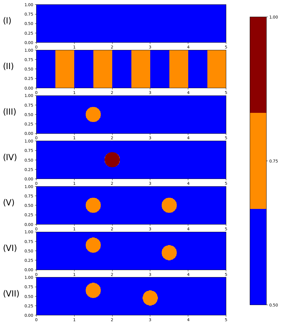
Figure 1: The different distribution of inhomogeneous fracture toughness that we consider. (I) homogeneous media, (II) stripe inclusion, (III-VII) disk inclusions. The color indicates fracture toughness; homogeneous media is shown in blue, whereas tougher inclusions are shown in red. One disk inclusions with (III) $\gamma_{1}=0.75$ and (IV) $\gamma_{1}=1.0$ are considered. Two disk inclusions with different positions in $x_{1}$ and $x_{2}$ are shown in (V-VII).

In order to study the difference among different geometry of inclusion and different toughness of the inclusion, we first consider the following four cases, namely (I) homogeneous toughness with $\gamma_{0}=0.5$; (II) periodic stripes whose toughness is $\gamma_{1}=0.75$ and the width of each region is 0.5; (III) one-disk inclusion with a disk whose barycenter is at $(1.5,0.5)$ with radius 0.2 and toughness $\gamma_{1}=0.75$; and (IV) one harder disk inclusion with disk’s barycenter at $(2.0,0.5)$ with radius 0.2 and $\gamma_{1}=1.0$. For the inhomogeneous materials, we set $\gamma_{0}=0.5$ outside the inclusion, which we call homogeneous media. We show the inhomogeneous distribution of $\gamma(\mathbf{x})$ in Fig. 1.

We should note that stripe inclusion and disk inclusion are inherently different because bypassing occurs only for the disk inclusion. We also remark that both in the simulations and in the estimation of fracture toughness, we neglect the interfacial effect of the inclusion, which was included in Lebihain et al. [10].

In addition to the four cases, we also consider three cases of two-disks inclusions with different positions. The inclusion disks’ coordinates are (V) $(1.5,0.5),(3.5,0.5)$; (VI) $(1.5,0.65),(3.5,0.45)$ and (VII) $(1.5,0.65),(3,0.45)$ with $\gamma_{1}=0.75$. Figure 1(V)-(VII) shows $\gamma({\bf x})$ for the three cases. These examples indicate that in (V) the two inclusions are placed at the center in the $x_{2}$ direction, and therefore the system has symmetry around the $x_{1}$ axis. In (VI) and (VII), the $x_{2}$ positions of the two inclusions are shifted from the center. Because the initial crack is chosen at the center of the $x_{2}$ axis and the crack goes straight in the homogeneous media, the crack reaches different positions on the surface of the inclusions. Therefore, the angle between the incoming crack to the inclusion, and line connecting the center of the inclusion and the its surface which the crack reaches, is different for each inclusion in (VI) and (VII). When the crack bypasses the inclusion, the crack path is expected to be deformed. The incoming angle of a crack reaching the second (right) inclusion may be changed by the distance between the two inclusions. We demonstrate it by using (VI) and (VII).

We perform numerical simulations of the phase-field models (4) and (5) by a finite volume method. We refer to [4] for the method as well as for the notation of the mesh. The discrete solution of $z$ and $u$ are denoted by $\{Z_{K}^{n}\}$ and $\{U_{K}^{n}\}$ over control volume $K$ in time interval $[t_{n},t_{n+1})$ respectively. We apply the uniform space mesh, which is the square size of $0.01\times 0.01$ and we apply uniform time discretization, that is we fix the time step to be $\Delta t=10^{-2}$ with $t_{n}=n\Delta t$ so that $[0,T)=\cup_{n=0}^{N_{T}-1}[t_{n},t_{n+1})$. We set the parameters as $\epsilon=0.02$ and $\mu=1$. For the surfing boundary condition, we first consider $v=1$ and $d=0.5$. We will specify the applied strain $A$ in each case.

Crack path and tip position in the $\mathrm{AT_{2}}$ model

We present the simulation results of the crack paths in the $\mathrm{AT_{2}}$ model, described in (4) with the initial condition as mentioned in [13]. The crack paths in the cases (I)-(IV) are shown in Fig.2. The crack paths are described by $z({\bf x})$. In the cases (I)-(III), the paths are straight, and therefore, penetration occurs for (II) and (III). On the other hand, the crack avoids in (IV), and it corresponds to bypassing. Figure 2 shows the crack paths in the cases (V)-(VII). In (V), the crack penetrates the two inclusions, whereas the crack avoids two inclusions in (VI). In (VII), the crack penetrates the right inclusion, but bypasses the left inclusion. It is clear that the shapes of crack paths are dependent both on the distribution of tougher regions, magnitude of the toughness, and their positions.

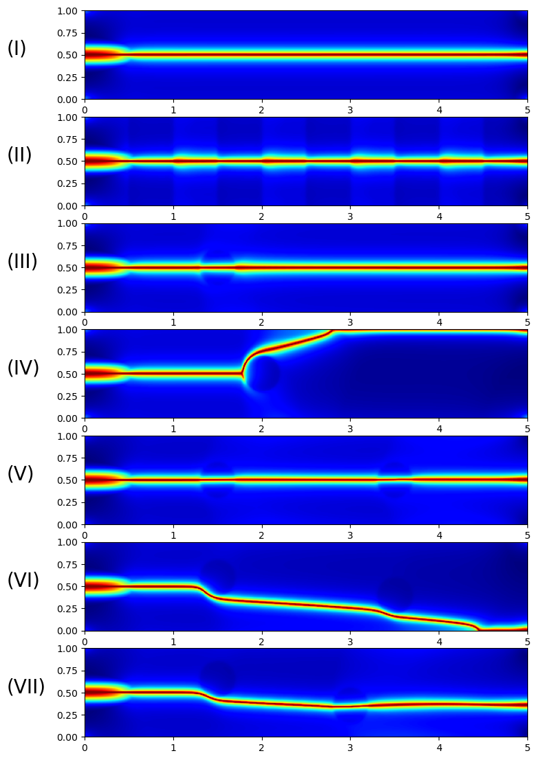
Figure 2: Crack paths in inhomogeneous materials with different spatial dependence of the fracture toughness $\gamma$ using the $\mathrm{AT_{2}}$ model. These paths correspond to the inhomogeneity in Fig. 1. The applied strain $A$ in (6) is chosen as $A=1.25$ for (I)-(IV), and $A=1$ for (V)-(VII).

As we will see later, the position of a crack tip, $x_{1}$, is an important observable for the $J$-integral computation and for the inverse problem, we therefore present the crack tip position in different cases. Figure 3 shows the position of a crack tip $x_{1}$ as a function of time. When the crack propagates in the homogeneous media, the speed of the propagation is approximately constant, and therefore, $x_{1}$ increases linearly in time. When the crack reaches an inclusion, the speed of the propagation decreases. After penetrating the inclusion, the speed of crack increases, and it becomes even higher than that of the crack in the homogeneous media. When the crack reaches a harder inclusion in Fig. 2(IV), the crack propagation stops, and when bypassing, the speed of the crack increases (see Fig. 3(IV)).

For the systems with two inclusions, the position of a crack tip $x_{1}(t)$ shows a similar behavior to the case of one inclusion. The speed of crack propagation slows down when it moves inside the inclusion, and the speed increases after penetration. In contrast with Fig. 2(IV), when the crack bypasses the inclusion as in Fig. 2(VI) and (VII), the speed does not change when the crack reaches the inclusion (Fig. 3(VI) and (VII)). This is because the incoming angle of the crack deviates from $\theta=0$. In this case, bypassing is more likely to occur, and accordingly, the crack does not get stuck when it reaches inclusion.

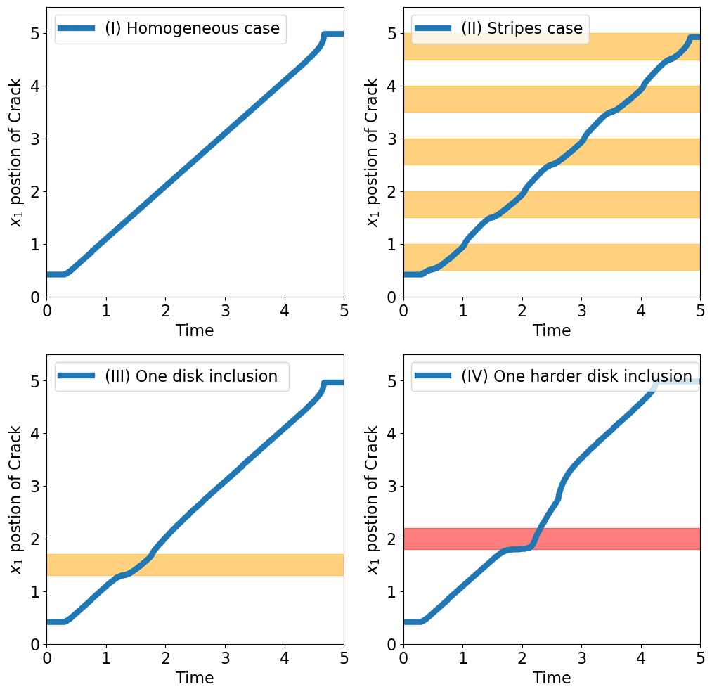
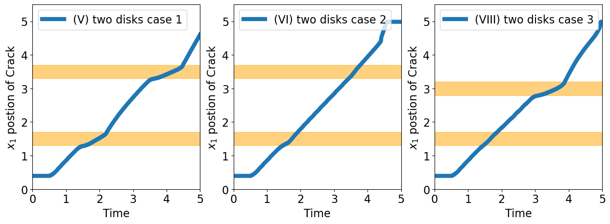
Figure 3: Positions of crack tips in $x_{1}$ as a function of time using the $\mathrm{AT_{2}}$ model. The shaded area corresponds to the inhomogeneity in Fig. 1.

Crack path and tip position in the $\mathrm{AT_{1}}$ model

Next, we consider the crack propagation in a heterogeneous media in the $\mathrm{AT_{1}}$ model. We use the same inhomogeneity as shown in Fig. 1 with the same surfing boundary conditions. The crack paths obtained by this model are qualitatively the same as those obtained by the $\mathrm{AT_{1}}$ model. The results are shown in Fig.4. In the case of (VII), the crack is eventually stuck at the right inclusion, and correspondingly $x_{1}$ saturates (see Fig. 5).

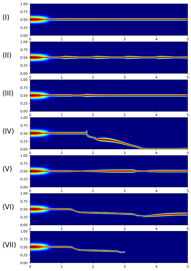
Figure 4: Crack paths in inhomogeneous materials with different spatial dependence of the fracture toughness $\gamma$ using the $\mathrm{AT_{1}}$ model. These paths correspond to the inhomogeneity in Fig. 1. The applied strain $A$ in (6) is chosen as $A=1.25$ for (I)-(IV), and $A=1$ for (V)-(VII).

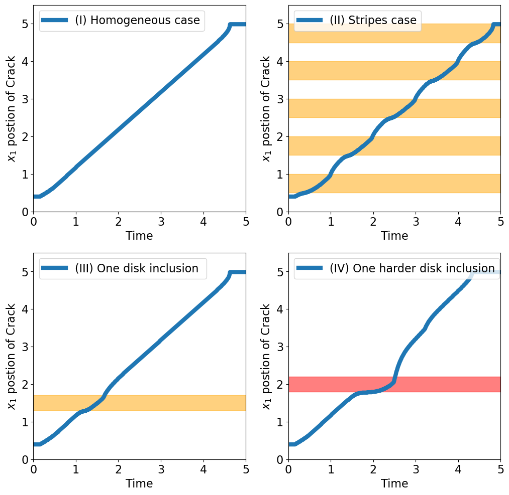
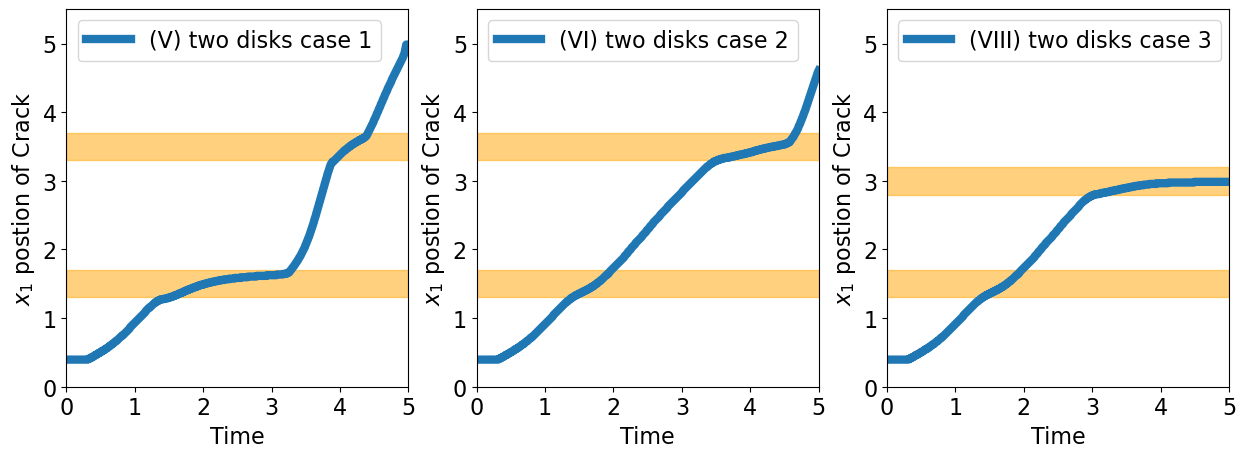
Figure 5: Positions of crack tips in $x_{1}$ as a function of time using the $\mathrm{AT_{2}}$ model. The shaded area corresponds to the inhomogeneity in Fig. 1.

3.2 characterization of effective toughness by $J$-integral during crack propagation

In the previous section, we observe different crack paths depending on the toughness of the inclusion, and its shape and geometry. In this section, we discuss effective toughness as a global property of the toughness of the heterogeneous material. For this purpose, we consider the $J$-integral. The $J$-integral is the strain energy release rate defined as

$$J: =-\frac{d(\mbox{Potential Energy)}}{d(\mbox{Crack Area})}$$

$$=\int_{{\Gamma_{J}}}\left({W}dy-{\mathbf{T}}\cdot\frac{\partial\mathbf{u}}{\partial x_{1}}ds\right),$$

where $\Gamma_{J}$ is an arbitrary counter-clockwise curve around the crack tip as shown in Fig. 6, $W$ is the strain energy density, and $\mathbf{T}=(T_{1},T_{2},T_{3})$ is the surface traction vector. For a homogeneous media, the $J$-integral corresponds to surface energy density $\gamma$ in (2) and (3). In this case, the $J$-integral is independent of the choice of the integration path $\Gamma_{J}$ [1]. On the other hand, in the inhomogeneous material, the $J$-integral is path-dependent.

We show the computation of the $J$-integral in the four cases (I)-(IV) that we consider in the Fig. 1. We choose the integration path $\Gamma_{J}$ in a counter-clockwise manner as in Fig. 6. Then, the $J$-integral is decomposed by the integral values on each boundary such that $J=J_{\Gamma_{1}}+J_{\Gamma_{2}}+J_{\Gamma_{3}}+J_{\Gamma_{4}}$. We refer to [2, 7] for the numerical computation of the $J$-integral both in homogeneous and inhomogenous systems using the phase-field model.

A direct computation yields

$$J_{\Gamma_{1}}=-\int_{\Gamma_{1}}(1-z)^{2}\left(\frac{\partial u}{\partial x_{2}}\right)^{2}dx_{2},$$ (7)

and

$$J_{\Gamma_{3}}=\int_{\Gamma_{3}}(1-z)^{2}\frac{\partial u}{\partial x_{2}}\frac{\partial u}{\partial x_{1}}ds,$$ (8)

and because of the symmetry, $J_{\Gamma_{4}}=J_{\Gamma_{3}}$. Because of the surfing boundary condition on $\Gamma_{3}$ and on $\Gamma_{4}$, when a crack propagates towards $\Gamma_{2}$, no strain will be applied on $\Gamma_{2}$, so that $J_{\Gamma_{2}}$ can be approximately ignored. When the crack approaches $\Gamma_{2}$, $J_{\Gamma_{2}}$ becomes nonzero, indicating that the finite system size affects the computation of the $J$-integral. Therefore, in the following, we present the computation of the $J$-integral before the moment $J_{\Gamma_{2}}$ starts to increase.

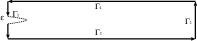
Figure 6: The contours $\Gamma_{J}$ for the computation of the $J$-integral. The cracked region is shown by the curve in the dotted line. The width of the region is $\sim\epsilon$ in (4) and (5).

The value of $J$-integral is sensitive to the choice of the position of $\Gamma_{1}$ because of the large value of ${\partial u}/{\partial y}$. We do not set $\Gamma_{1}$ to be the boundary $\{x_{1}=0\}\times(0,H)$ of the domain because the initial condition do not satisfy the equation. In the following, both in $\mathrm{AT_{2}}$ and $\mathrm{AT_{1}}$ models, we set the position of $\Gamma_{1}$ to be $49\Delta x$.

Figure 7 shows the $J$-integral during propagation. We normalize the $J$-integral by the value for the homogeneous media at $t=100\Delta t$ to see the dependence on the toughness $\gamma$ in the inclusion. For the homogeneous media ((I) in Fig.1), the $J$-integral is constant in time. This result is consistent with the constant speed of crack propagation. When the crack propagates in tough inclusions ((II)-(IV) in Fig.1)), the $J$-integral increases. After going out from the inclusions, the $J$-integral decreases to the value of the homogeneous media. In the case of (II) and (III), the maximum value is approximately $\gamma$ of the tougher regions, $\gamma_{1}/\gamma_{0}\approx 1.5$. When the toughness of the inclusion is larger, the maximum value of the $J$-integral is larger.

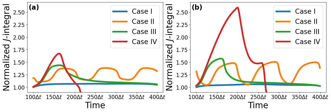
Figure 7: The $J$-integral during crack propagation in inhomogeneous media using the (A) $\mathrm{AT_{2}}$ and (B) $\mathrm{AT_{1}}$ models corresponding to Fig. 1(I)-(IV). The applied strain $A$ in (6) is chosen as $A=1.25$.

To study how inhomogeneous toughness affects crack propagation, we focus on the cases of the one-disk inclusion whose toughness is gradually increased from $0.75$ to $1.0$. We start from $\mathrm{AT_{2}}$ model with a disk inclusion at $(1.5,0.5)$ with radius 0.2. The toughness of the inclusion is $0.75,0.8,0.85,0.9,0.95$ to $1$ with the $A$ in the surfing boundary condition to be $1$. We find that the crack path changes from penetration to pinning as the toughness of the inclusion increases, as shown in Fig. 8. When $\gamma=1$ and $A=1.25$, the crack path shows bypassing after pinning at the surface of the inclusion. We then consider $\mathrm{AT_{1}}$ model with $A=1.25$. We find that the crack paths change from straight penetration to deviated penetration as the toughness of the inclusion increases.

The results of corresponding $J$-integrals to each path in Fig. 7 are shown in Fig.8. In both models, the peak value of $J$-integral increases as $\gamma_{1}$ in the disk inclusion increases. Before the $J$-integral reaches the value comparable with $\gamma_{1}/\gamma_{0}$, the crack is pinned at the surface of the inclusion. When $\gamma_{1}/\gamma_{0}$ is small, the crack starts to move after reaching the peak, and results in penetration. On the other hand, when $\gamma_{1}/\gamma_{0}$ is large, the $J$-integral saturates and the crack remains at the pinned state. When the applied strain is larger $A=1.25$ in Fig.8(a), the $J$-integral increases as the crack tip hits the disk and is pinned before bypassing occurs. After the crack starts to move. The $J$-integral reaches its peak and takes a larger value than $\gamma_{1}/\gamma_{0}$. After the crack starts to move, the $J$-integral drops. The crack path is no longer along the $x_{1}$ direction, and therefore, the $J$-integral does not come back to the value of the inhomogeneous media. These behaviors are shared both by the $\mathrm{AT_{1}}$ and $\mathrm{AT_{2}}$ models.

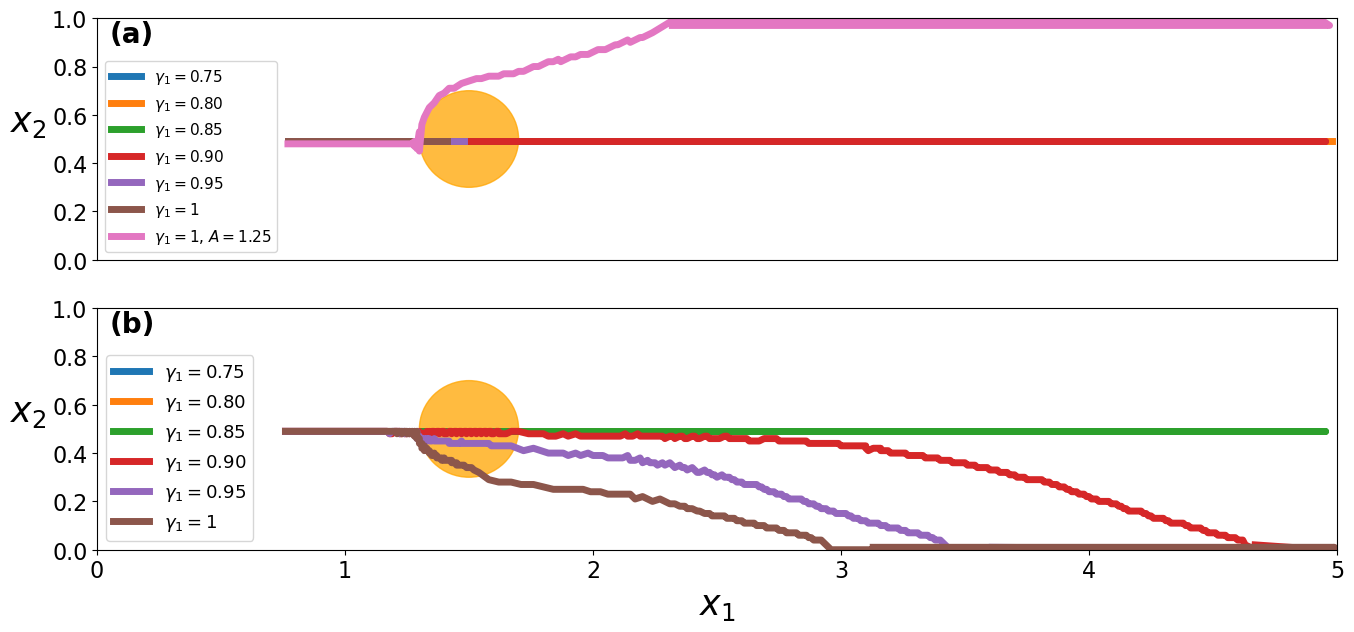
Figure 8: The crack paths obtained by the tip positions $(x_{1},x_{2})$ in the inhomogeneous media under different toughness $\gamma_{1}$. The results of the (a) $\mathrm{AT_{2}}$ and (b) $\mathrm{AT_{1}}$ models are shown. The applied strain $A$ of (6) is chosen as $A=1$ in (a) and $A=1.25$ in (b).

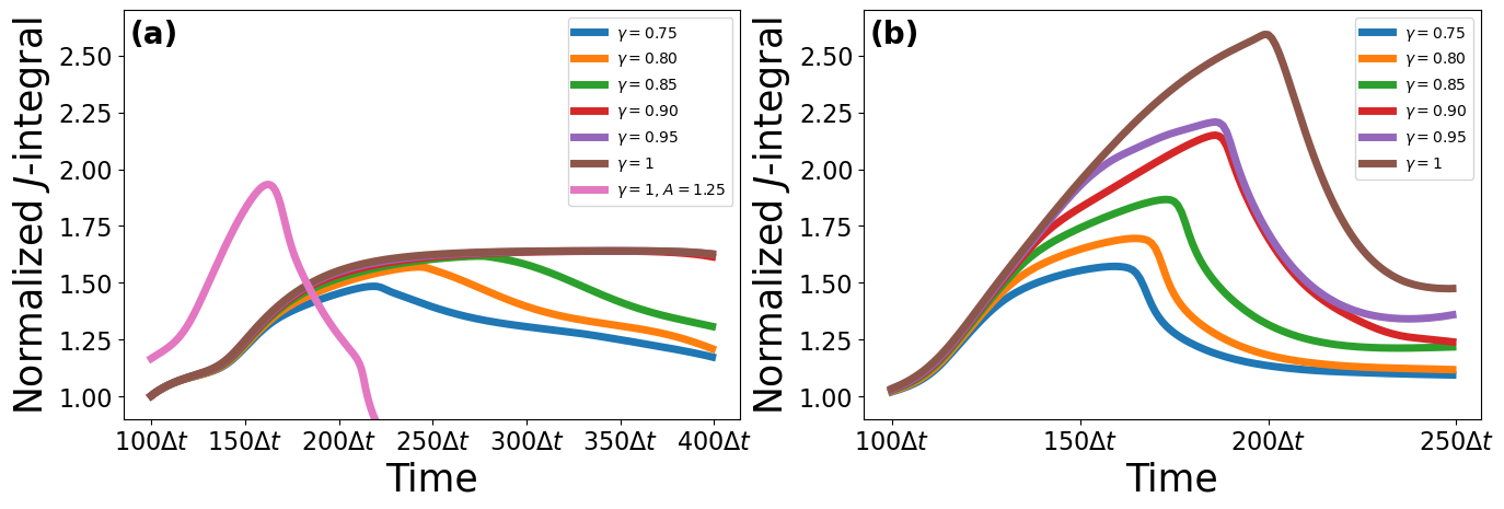
Figure 9: The $J$-integral during crack propagation in the inhomogeneous media under different toughness $\gamma_{1}$ corresponding to Fig. 8. The results of the (a) $\mathrm{AT_{2}}$ and (b) $\mathrm{AT_{1}}$ models are shown. The applied strain $A$ of (6) is chosen as $A=1$ in (a) and $A=1.25$ in (b).

Despite the similar results of the $\mathrm{AT_{1}}$ and $\mathrm{AT_{2}}$ models, there are differences between these models. In Fig. 10, we check the shape of the solutions. Given a time $t^{n}$, we obtain the simulation result of $z(x_{1},x_{2})$, then fix the $x_{1}$ coordinates and plot the solution of $z$ as a function of $x_{2}$ coordinates. We find that for the solution in the $\mathrm{AT_{2}}$ model, the values on $\{x_{2}=0,x_{2}=1\}$, which correspond to the boundary $\Gamma_{3}$ and $\Gamma_{4}$, are not $0$. The difference was also discussed in Tanne et al. [12] and Wu et al. [14]. In Wu et al. [14], the authors show the distribution of the crack phase-field in different models. In our notation, the solution is approximated, for fixed $x_{1}$, as $z=(1-\frac{|x_{2}|}{2l_{0}})^{2}$ in $\mathrm{AT_{1}}$, whereas $z=\exp(-\frac{|x_{2}|}{l_{0}})$ in $\mathrm{AT_{2}}$, where $l_{0}$ is the length scale. This is also shown in our case in Figure 10. Accordingly, the effect of the plus operator is very different in the two models, that is in $\mathrm{AT_{1}}$, the effect is over the whole domain, whereas in $\mathrm{AT_{2}}$, the effect is mainly on the region where the value of $z$ is large. This difference may affect the inverse estimation of the fracture toughness that we present in Sec. 4.

Figure 10: The cross sections along $x_{2}$ of the crack field $z(x_{2})$ in the homogeneous media using the $\mathrm{AT_{2}}$ and $\mathrm{AT_{1}}$ models at time $t=174\Delta t$.

4 Estimation of fracture toughness

The aim of this section is to propose and demonstrate the method to estimate the fracture toughness $\gamma$ from the crack path obtained from the phase-field model. More precisely, we perform simulation for the phase-field models, and apply a regression technique on numerical results $\{Z_{K}^{n}\}$ and $\{U_{K}^{n}\}$ to estimate $\gamma$. The basic idea is to optimise $\gamma$ so that the left-hand and right-hand sides of (4) or (5) become closer in a certain norm. This is not straightforward as it looks because of the nonlinearlity caused by the $(\cdot)_{+}$ operator. In fact, when the $(\cdot)_{+}$ operator works, (4) and (5) without $(\cdot)_{+}$ operator are not equality but inequality. Therefore, we cannot use all the sample points in the system, but need pre-process to choose appropriate sample points.

4.1 inverse problems of the $\mathrm{AT_{2}}$ model

We start from the model of $\mathrm{AT_{2}}$, and we propose the following algorithm.

1. Simulation: We perform the simulation of the phase-field model of $\mathrm{AT_{2}}$. At the same time, we track the position of the crack tip at each time step. We denote the position of the crack tip as $(x_{1,n},x_{2,n})$ at time step $n\Delta t$ for all $1\leq n\leq N_{T}$.

2. Sampling: At each time step, we sample the grid points in space in the region where the crack has not arrived. We consider the time interval $[n_{0}\Delta t,n_{1}\Delta t)$. We define $\Omega_{n}=[x_{1,n},L]\times[0,H]$, that is the space region where the crack has not arrived yet. And then we sample $N_{x_{1}}$ grid points over $[x_{1,n},L]$ and $N_{x_{2}}$ grid points on $[0,H]$. The $j^{th}$ sample point will be denoted by $p_{j}:=((x_{1}^{(j)},x_{2}^{(j)}),t^{(j)})$ and the total sample set is denoted by $P=\{p_{j}\}_{j=1,2,...,N_{data}}$ with $N_{data}=(n_{1}-n_{0})\cdot N_{x_{1}}\cdot N_{x_{2}}$.

3. Interpolation: We apply Chebyshev polynomial of degree $7$ for the interpolation of $\{Z(P)\}$ and $\{U(P)\}$. The results of the interpolation is denoted by $\widetilde{Z}(x_{1},x_{2},t)$ and $\widetilde{U}(x_{1},x_{2},t)$. Then, by computing the derivative of the polynomial, we obtain the values of $\displaystyle{{\partial\widetilde{Z}}/{\partial t}}$, $\displaystyle{{\partial\widetilde{Z}}/{\partial{x_{1}}}}$, $\displaystyle{{\partial\widetilde{Z}}/{\partial{x_{2}}}}$, $\Delta\widetilde{Z}$ and $\lvert\nabla\widetilde{U}\rvert^{2}(1-\widetilde{Z})$.

4. Linear Regression: We assume that the values of $\alpha_{2}$, $\epsilon$, and $\mu$ are known and that $\gamma$ is constant, which corresponds to the homogeneous material. Based on the second equation of system (4), if we omit the plus operator $(\cdot)_{+}$, formally we obtain

   $$\alpha_{2}\frac{\partial\widetilde{Z}}{\partial t}=\gamma\left(\epsilon\Delta\widetilde{Z}-\frac{\widetilde{Z}}{\epsilon}\right)+\mu\lvert\nabla\widetilde{U}\rvert^{2}(1-\widetilde{Z}),$$ (9)

   from which we define

   $$Y:=\alpha_{2}\frac{\partial\widetilde{Z}}{\partial t}-\mu\lvert\nabla\widetilde{U}\rvert^{2}(1-\widetilde{Z})$$ (10)

   and

   $$X:=\epsilon\Delta\widetilde{Z}-\frac{\widetilde{Z}}{\epsilon}.$$ (11)

   If we find the linear relation such that $Y=\hat{\gamma}X$, then $\hat{\gamma}$ is the estimator of $\gamma$, that is the fracture toughness of the phase-field model. We will generalize this approach to the inhomogeneous $\gamma$.

4.1.1 homogeneous case

We start from the numerical results of a homogeneous material with $\gamma_{0}=0.5$. We consider the time interval $[100\Delta t,200\Delta t)$ and at each time step we sample $20\times 20$ the grid points. The positions of sample points are shown in Fig. 11. Based on the sample points, we perform interpolation and compute time and spatial derivatives of $Z$ to evaluate $X$ and $Y$. The results are shown in Fig. 11. Applying the linear regression, we obtain $Y=0.5002\cdot X$. The ground truth of $\gamma_{0}$ is $\gamma_{0}=0.5$, and thus we obtain an accurate estimation.

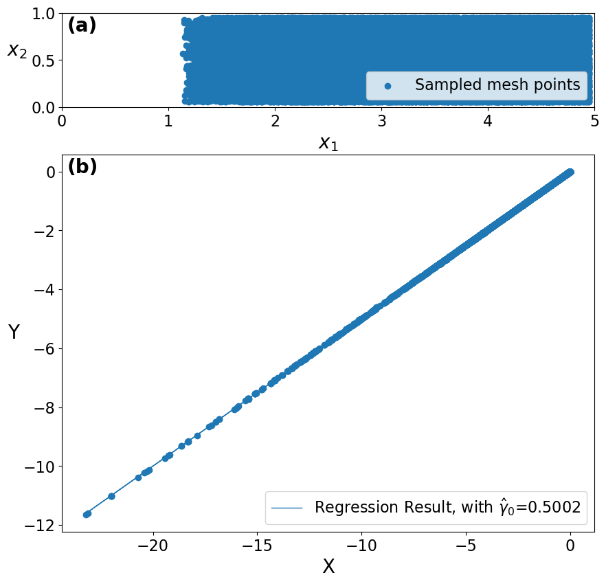
Figure 11: (a) Sampled grid points at which crack has not yet arrived. (b) The sampled data points in $(X,Y)$ of (11) and (10). The solid line is the result of linear regression. The applied strain $A$ in (6) is chosen as $A=1.25$.

4.1.2 Inhomogeneous case

In the inhomogeneous case, the fracture toughness $\gamma(x)$ is non-uniform in space. Therefore, we expand $\operatorname{div}(\gamma(x)\nabla z)$ and omit the plus operator $(\cdot)_{+}$ in (4) to obtain

$$\alpha_{2}\frac{\partial\widetilde{Z}}{\partial t}= \gamma(x)\left(\epsilon\Delta\widetilde{Z}-\frac{\widetilde{Z}}{\epsilon}\right)+\mu\lvert\nabla\widetilde{U}\rvert^{2}(1-\widetilde{Z})$$ (12)

$$+\epsilon\frac{\partial\gamma(x)}{\partial{x_{1}}}\cdot\frac{\partial\widetilde{Z}}{\partial{x_{1}}}+\epsilon\frac{\partial\gamma(x)}{\partial{x_{2}}}\cdot\frac{\partial\widetilde{Z}}{\partial{x_{2}}}.$$

Similar to step 4 of the homogeneous case, we define

$$Y:=\alpha_{2}\frac{\partial\widetilde{Z}}{\partial t}-\mu\lvert\nabla\widetilde{U}\rvert^{2}(1-\widetilde{Z})$$

and

$$X:=\epsilon\Delta\widetilde{Z}-\frac{\widetilde{Z}}{\epsilon},\quad X_{1}:=\epsilon\frac{\partial\widetilde{Z}}{\partial{x_{1}}},\quad X_{2}:=\epsilon\frac{\partial\widetilde{Z}}{\partial{x_{2}}}.$$

Because we consider the inclusion that has larger value of $\gamma$, which is sharply varied from the value in the media, the terms ${\partial\gamma(x)}/{\partial{x_{1}}}$ and ${\partial\gamma(x)}/{\partial{x_{2}}}$ approximately vanish at the many sample points. Therefore, we may apply the regression using $Y$ and $X$ to analyse the inhomogeneity in the same way as we did in the homogeneous case.

We assume that the fracture toughness $\gamma$ can take two values; $\gamma_{0}$ in the media and $\gamma_{1}$ in an inclusion. Although each sample point of $(X,Y)$ does not know whether this point is $\gamma_{0}$ or $\gamma_{1}$, we may classify each point using the method of modified $k$-means (see Appendix A. $k$-means algorithm for the detailed method). As in the homogeneous case, the grid points are sampled in the region where the crack has not arrived in each case.

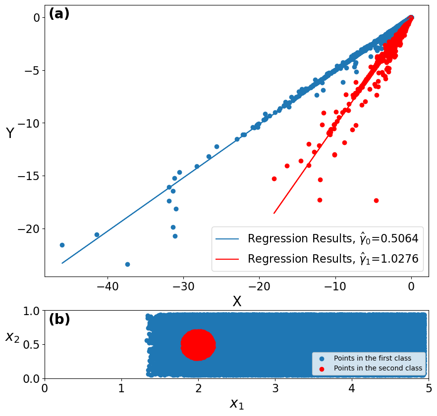
Figure 18: (a) The sampled data in $(X,Y)$ obtained by the $\mathrm{AT_{2}}$ model for the crack propagation in inhomogeneous media with a harder disk inclusion. The data is classified by using the $k$-means algorithm. The solid line is the result of linear regression for each class. (b) The positions of the data point corresponding to each class. The applied strain $A$ in (6) is chosen as $A=1.25$.

Similar to Sec.3, we consider the inhomogeneity of case (II)-(VII) in Fig. 1. We choose the time interval to be $[100\Delta t,200\Delta t)$, except the case (IV) in which we consider the time interval $[120\Delta t,200\Delta t)$ because the position of the inclusion is $x_{1}=2.0$ ( see Fig. 18).

Figure 12: (a,b) The sampled data in $(X,Y)$ for the crack propagation in inhomogeneous media with stripe inclusions before (a) and after (b) the classification using the $k$-means algorithm. The solid line in (b) is the result of linear regression for each class. (c,d) The positions of the data point in real space before (a) and after (b) the classification. The applied strain $A$ in (6) is chosen as $A=1.25$.

We first consider the stripe inclusions. We show in Fig. 12(a) the results of $X$ and $Y$ after sampling and interpolation. The result indicates that there are two slopes. In fact, by applying $k$-means, we may classify the points and estimate the $\gamma$ in each class. The estimated values of $\gamma$ are $\hat{\gamma}_{0}=0.5016$ and $\hat{\gamma}_{1}=0.7501$ which are close to the ground truth, $0.5$ and $0.75$. In Fig.12, we show the spatial position of the points in the two classes. The result shows a good agreement with the spatial distribution of $\gamma(x)$ in Fig.1(II). This result suggests that the method can discover not only the different values of the inhomogeneity, but also the position of the inhomogeneity.

Next, we consider the one-disk inclusion. In Fig.13(a,b), we show the results of the sampling after interpolation and $k$-means method are applied. The estimated values of $\gamma$ are $\hat{\gamma}_{0}=0.5008$ and $\hat{\gamma}_{1}=0.7534$ compared to $0.5$ and $0.75$ of the ground truth. Our method also works for the disk inclusion with harder toughness (Fig.1(IV)). The estimated values of $\gamma$ are $\hat{\gamma}_{0}=0.5064$ and $\hat{\gamma}_{1}=1.0276$ compared to their ground truth values $0.5$ and $1.0$, respectively. The result is shown in Fig. 18 in Supplementary Materials.

Our method to estimate the toughness $\gamma$ of inclusions and their positions also work for multiple inclusions. We consider the three cases (V-VII) in Fig.1. Figure 13(c,d) show the results of the case (V) after the pre-processing of data, interpolation and $k$-means method as mentioned in the algorithm. The results show that we could accurately estimate two $\gamma$ corresponding to the toughness of media , $\gamma_{0}$, and inclusions, $\gamma_{1}$. The estimated toughness is $\hat{\gamma_{0}}=0.4963$ and $\hat{\gamma_{1}}=0.7562$. Note that in this case, the crack penetrates both inclusions (see Fig. 2).

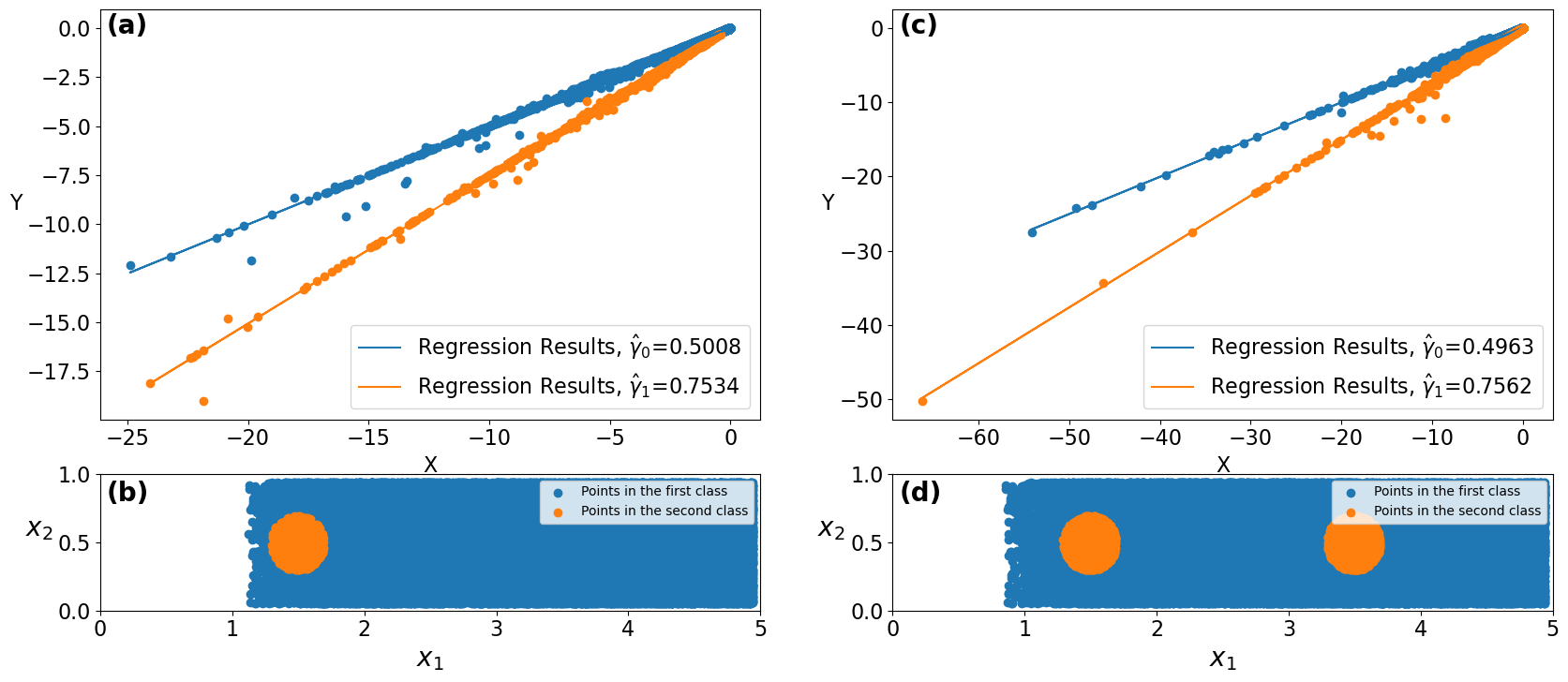
Figure 13: Propagation in inhomogeneous media with a disk inclusion after the classification using the $k$-means algorithm. The solid line is the result of linear regression for each class. (b) The positions of the data point corresponding to each class. (c) The sampled data in $(X,Y)$ for the crack propagation in inhomogeneous media with two disk inclusions after the classification using the $k$-means algorithm. The solid line is the result of linear regression for each class. (d) The positions of the data point corresponding to each class. The applied strain $A$ in (6) is chosen as $A=1.25$ for (a,b) and $A=1$ for (c,d).

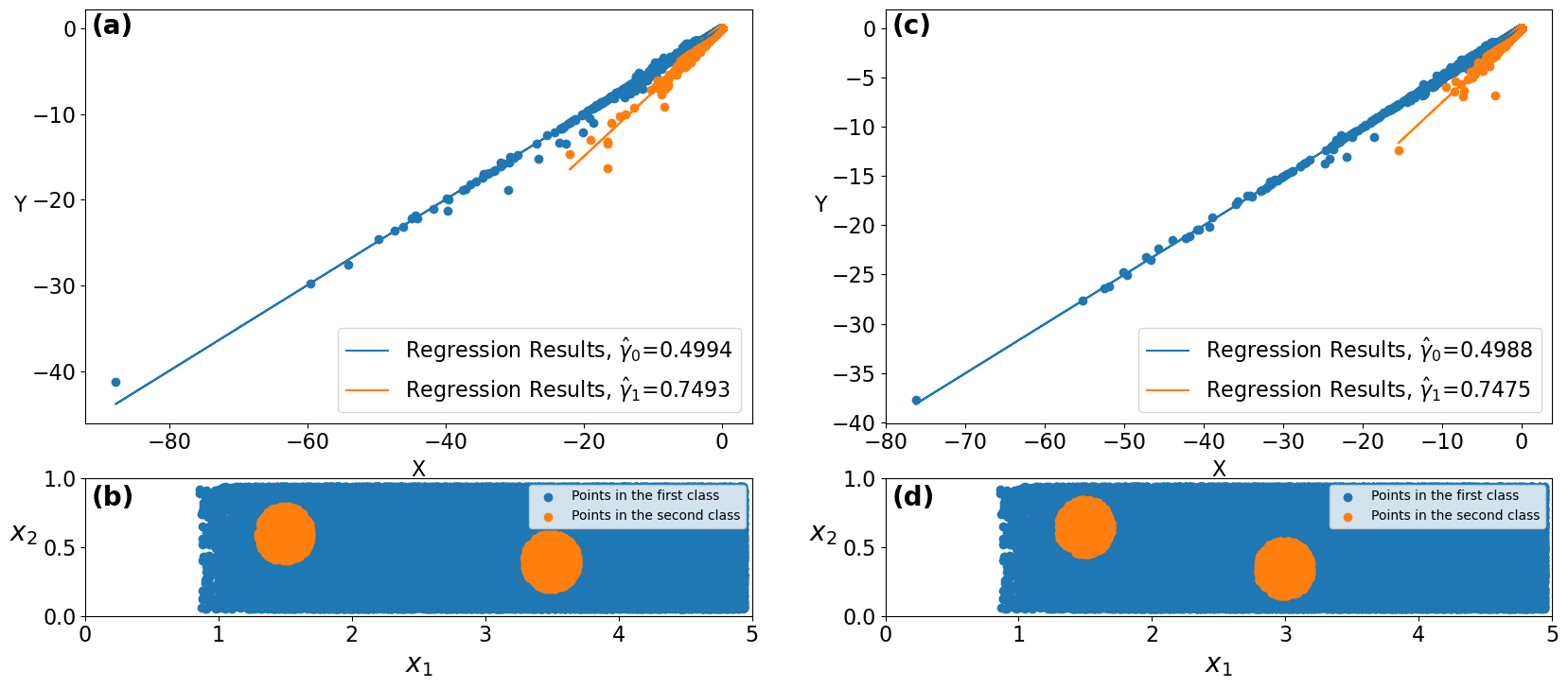
Figure 19: (a) The sampled data in $(X,Y)$ obtained by the $\mathrm{AT_{2}}$ model for the crack propagation in inhomogeneous media with two disk inclusions. The data is classified by using the $k$-means algorithm. The solid line is the result of linear regression for each class. (b) The positions of the data point corresponding to each class. (c) The sampled data in $(X,Y)$ obtained by the $\mathrm{AT_{2}}$ model for the crack propagation in inhomogeneous media with two disk inclusions. The data is classified by using the $k$-means algorithm. The solid line is the result of linear regression for each class. (d) The positions of the data point corresponding to each class. The applied strain $A$ in (6) is chosen as $A=1$.

Our method successfully estimate the toughness of inclusions at different positions. In the cases (VI) and (VII) in Fig.2, the crack bypasses the inclusions (VI), or it bypass one inclusions and is stuck at the second inclusion. Due to the bypassing, the number of data points corresponding to the inclusions is small. Still, we may estimate the toughness as $\hat{\gamma}_{0}=0.4994$ and $\hat{\gamma}_{1}=0.7493$ for the case (VI), and $\hat{\gamma}_{0}=0.4988$ and $\hat{\gamma}_{0}=0.7475$ for the case (VII). We may also estimate the position of the inclusions as shown in Fig.19 in Supplementary Materials.

We should stress that we use the data before the crack reaches the second inclusion in the case of two disk inclusions (see Fig. 3(v)-(vii) with the time interval $[100\Delta t,200\Delta t)$. Therefore, we may predict the position and toughness of the second inclusion.

4.2 inverse problems of the $\mathrm{AT_{1}}$ model

Next we consider the phase-field model (5), which is based on the surface energy $\mathrm{AT_{1}}$. Naively, we may apply the same algorithm as in section 4.1 and change the corresponding definitions in step 4, the Linear Regression. However, as we will see, this naive method does not work for the $\mathrm{AT_{1}}$ model. This is because in this model, the plus operator $(\cdot)_{+}$ is effective almost everywhere in space except near the crack tip. Therefore, we need additional pre-processes to estimate the toughness in this model.

We assume that the values of $\alpha_{2}$, $\epsilon$, and $\mu$ are known. Based on the second equation of system (5), if we omit the plus operator $(\cdot)_{+}$, formally we obtain

$$\alpha_{2}\frac{\partial\widetilde{Z}}{\partial t}=\gamma\left(\frac{3}{4}\epsilon\Delta\widetilde{Z}-\frac{3}{8\epsilon}\right)+\mu\lvert\nabla\widetilde{U}\rvert^{2}(1-\widetilde{Z}).$$ (13)

This leads us to define

$$Y:=\alpha_{2}\frac{\partial\widetilde{Z}}{\partial t}-\mu\lvert\nabla\widetilde{U}\rvert^{2}(1-\widetilde{Z})$$

and

$$X:=\frac{3}{4}\epsilon\Delta\widetilde{Z}-\frac{3}{8\epsilon}.$$ (14)

If we find the linear relation such that $Y=\hat{\gamma}X$, then $\hat{\gamma}$ is the estimator of $\gamma$, that is the fracture toughness of the phase-field model.

4.2.1 homogeneous case

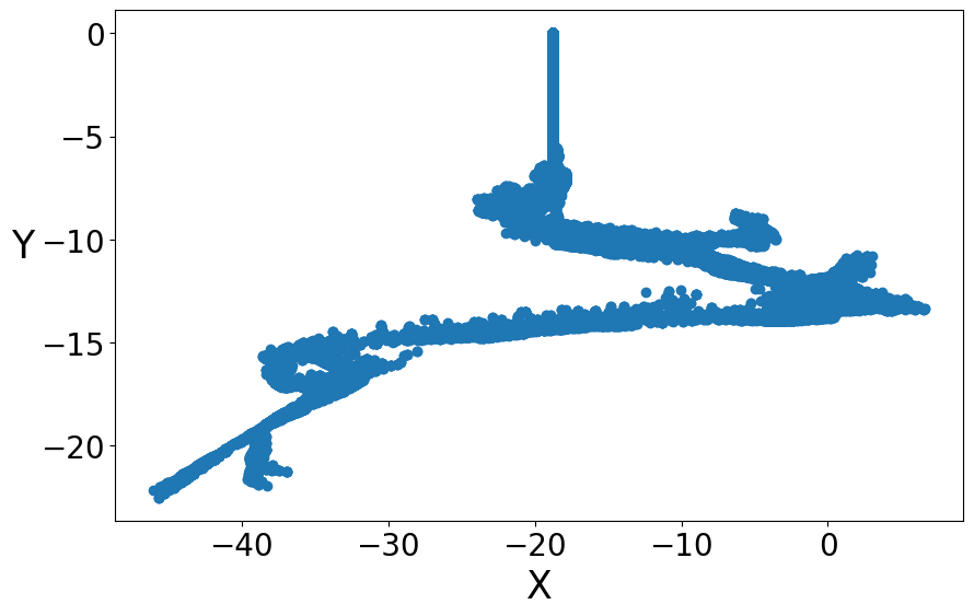
Figure 17: The sampled data in $(X,Y)$ for the crack propagation in homogeneous media using the $\mathrm{AT}_{1}$ model, using the same algorithm for the $\mathrm{AT}_{2}$ model.

We first perform the estimation of the homogeneous case by using the same algorithm as in the Section 4.1. The sampled data is shown in Fig. 17 in the Supplementary Materials. The deviation is due to the plus operator $(\cdot)_{+}$. In fact, when the right-hand side of (13) is negative, the crack field $\widetilde{Z}$ does not satisfy (13) but $\partial\widetilde{Z}/\partial t=0$. This occurs particularly when $\widetilde{Z}$ and $\widetilde{U}$ are uniform in space, corresponding to the points away from the crack tip. The difference from the $\mathrm{AT_{2}}$ originates from the second term in (11) and (14). When $\widetilde{Z}\approx 0$, $X\approx 0$ in (11) and accordingly the right-hand side of (9) is approximately 0. On the other hand, in the $\mathrm{AT_{1}}$ when $\widetilde{Z}\approx 0$, $X<0$ and the right-hand side of (13) becomes negative if $\widetilde{U}$ is approximately uniform in space. In this case, $X$ and $Y$ do not exhibit a linear relationship due to the plus operator.

We, therefore, propose an additional pre-process of the data. Inspired by the form of the solution in Fig. 10, we propose to sample the points at the region where the values of $z$ are closer to $1$. Given a time interval $[n_{0}\Delta t,n_{1}\Delta t)$, at each time step, we consider the region where the crack has not arrived, similar to the estimation for the $\mathrm{AT_{2}}$ model. We denote the tip position at $n\Delta t$ to be $(x_{1,n},x_{2,n})$ and define $\Omega_{n}=[x_{1,n},x_{1,n}+\Delta x]\times[x_{2,n},x_{2,n}+\Delta y]$, that is a small disk containing four points around the crack tip. As we use the uniform square mesh, the sample points correspond to one-fourth of a disk whose radius $r$ satisfies $(\sqrt{5}/2)\Delta x<r<(3/2)\Delta x$.

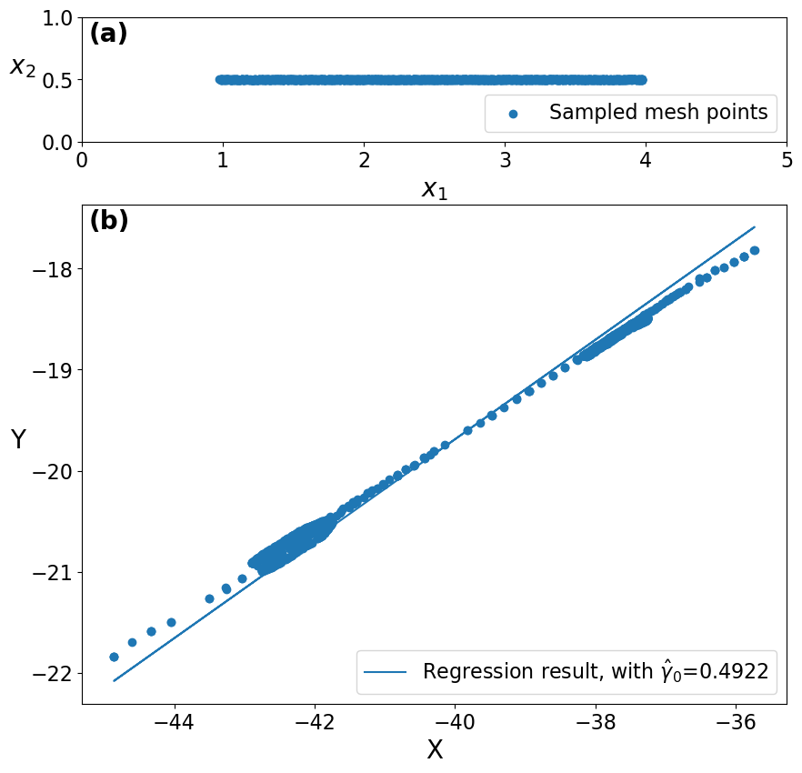
Figure 14: (a) The positions of the data point obtained by the $\mathrm{AT_{1}}$ model after pre-processing. (b) The sampled data in $(X,Y)$ for the crack propagation in homogeneous media using the $\mathrm{AT_{1}}$ model. The solid line is the result of linear regression. The applied strain $A$ in (6) is chosen as $A=1.25$.

We consider the time interval $[n_{0}\Delta t,n_{1}\Delta t)$. The $j^{th}$ sample point will be denoted by $p_{j}:=((x_{1}^{(j)},x_{2}^{(j)}),t^{(j)})$ and the total sample set is denoted by $P=\{p_{j}\}_{j=1,2,...,N_{data}}$ with $N_{data}=(n_{1}-n_{0})\cdot 2\cdot 2$. The sampled data points of the time interval $[80\Delta t,380\Delta t)$ for the homogeneous media are shown in Fig. 14(a). We note that the crack path is a straight line in the homogeneous material case (see Fig.2). In contrast with the estimation of $\mathrm{AT_{2}}$ model, the number of data points is small and limited to the region near the crack path. Therefore, the estimation of the toughness and positions of inclusions are much harder in $\mathrm{AT_{1}}$ model.

We compute the $X$ and $Y$ on the chosen data set. The result is shown in Fig. 14(b). By applying the linear regression, we can estimate $\hat{\gamma}=0.4922$, which is comparable with the ground truth $\gamma=0.5$. Despite the small number of sample points, our method successfully estimate the toughness of the homogeneous media in the $\mathrm{AT_{1}}$ model.

4.2.2 Inhomogeneous case

For the inhomogeneous materials in the $\mathrm{AT_{1}}$, we apply the $k$-means as in Sec. 4.1.2 to divide the data into two classes corresponding to two toughness $\gamma_{0}$ and $\gamma_{1}$. We also have to use the pre-processing the data points as in Sec. 4.2.1. We consider the time interval to be $[80\Delta t,380\Delta t)$ for the cases (II) and (III), $[80\Delta t,300\Delta t)$ for the case (IV) and $[80\Delta t,480\Delta t)$ for the cases (V)-(VII).

Figure 15(a) shows the data after pre-processing for the data of crack propagation in the inhomogeneous media with the stripe inclusions. We may see the data can be decomposed into two classes. In fact, by applying $k$-means, we find two classes corresponding to two toughness, $\gamma_{0}$ in the homogeneous media and $\gamma_{1}$ in the inclusions. The regression results show $\hat{\gamma}_{0}=0.5037$ and $\hat{\gamma}_{1}=0.751$. They are reasonably closed to the ground truth $\gamma_{0}=0.5$ and $\gamma_{1}=0.75$.

The data points in each class are located at $\gamma_{0}$ or $\gamma_{1}$ as shown in Fig. 15(b). We are able to discover the $x_{1}$ position of the inhomogeneous part. However, in contrast with the estimation shown in Sec. 4.1, we cannot identify all the position of the inhomogeneity. This is because the effect of the plus operator is stronger in the $\mathrm{AT_{1}}$ model than the $\mathrm{AT_{2}}$ model. We cannot use the data points at which the plus operator works. Therefore, we lose many data points in the $\mathrm{AT_{1}}$ model. Still, we may find the position of tougher regions using our estimation method.

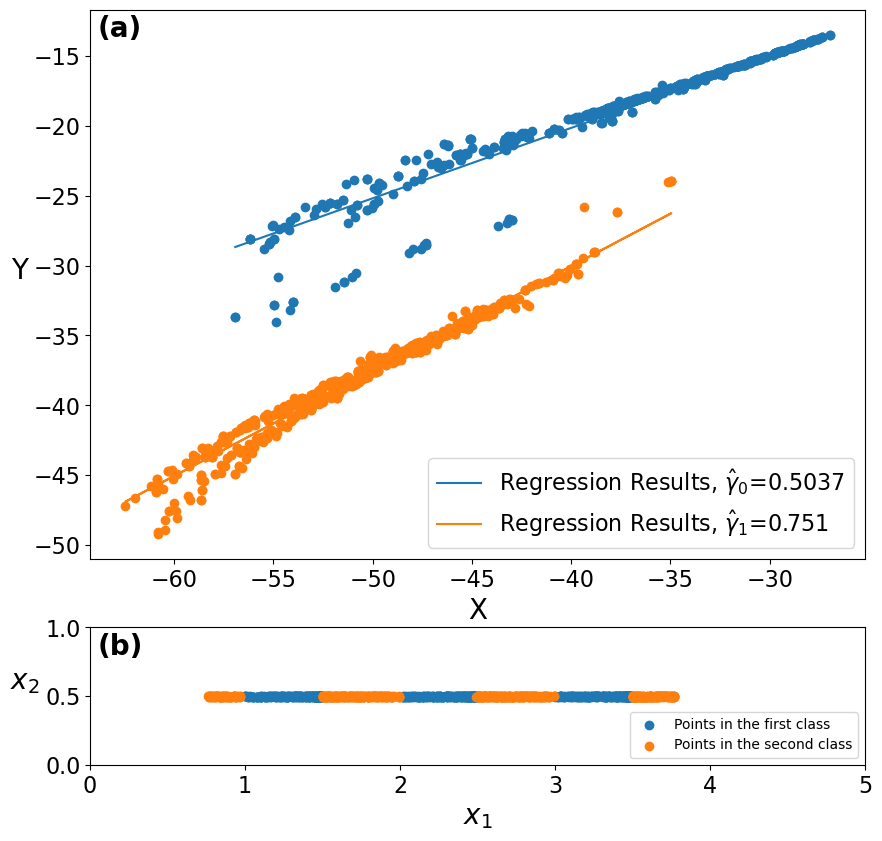
Figure 15: (a) The sampled data in $(X,Y)$ obtained by the $\mathrm{AT_{1}}$ model for the crack propagation in inhomogeneous media with stripe inclusions after the classification using the $k$-means algorithm. The solid line is the result of linear regression for each class. (b) The positions of the data point corresponding to each class. The applied strain $A$ in (6) is chosen as $A=1.25$.

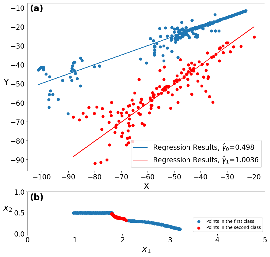
Figure 20: (a) The sampled data in $(X,Y)$ obtained by the $\mathrm{AT_{1}}$ model in the time interval $[80\delta t,300\delta t)$ for the crack propagation in inhomogeneous media with a harder disk inclusion. The data is classified by using the $k$-means algorithm. The solid line is the result of linear regression for each class. (b) The positions of the data point corresponding to each class. The applied strain $A$ in (6) is chosen as $A=1.25$.

Figure 16(a) shows the results of estimation for one-disk inclusion. The regression results show $\hat{\gamma}_{1}=0.4934$ and $\hat{\gamma}_{2}=0.7471$. Figure 16(b) shows the points of $\gamma_{0}$ and $\gamma_{1}$ in the $x_{1}-x_{2}$ space. We can estimate the position of $x_{1}$ coordinates of the inhomogenous part, that is the disk inclusion. We recall the the inclusion is a disk with barycenter $(1.5,0.5)$ and radius 0.2. The estimation also works for the one harder disk inclusion in the $\mathrm{AT_{1}}$ model as shown in Fig.20 in Supplementary Materials.

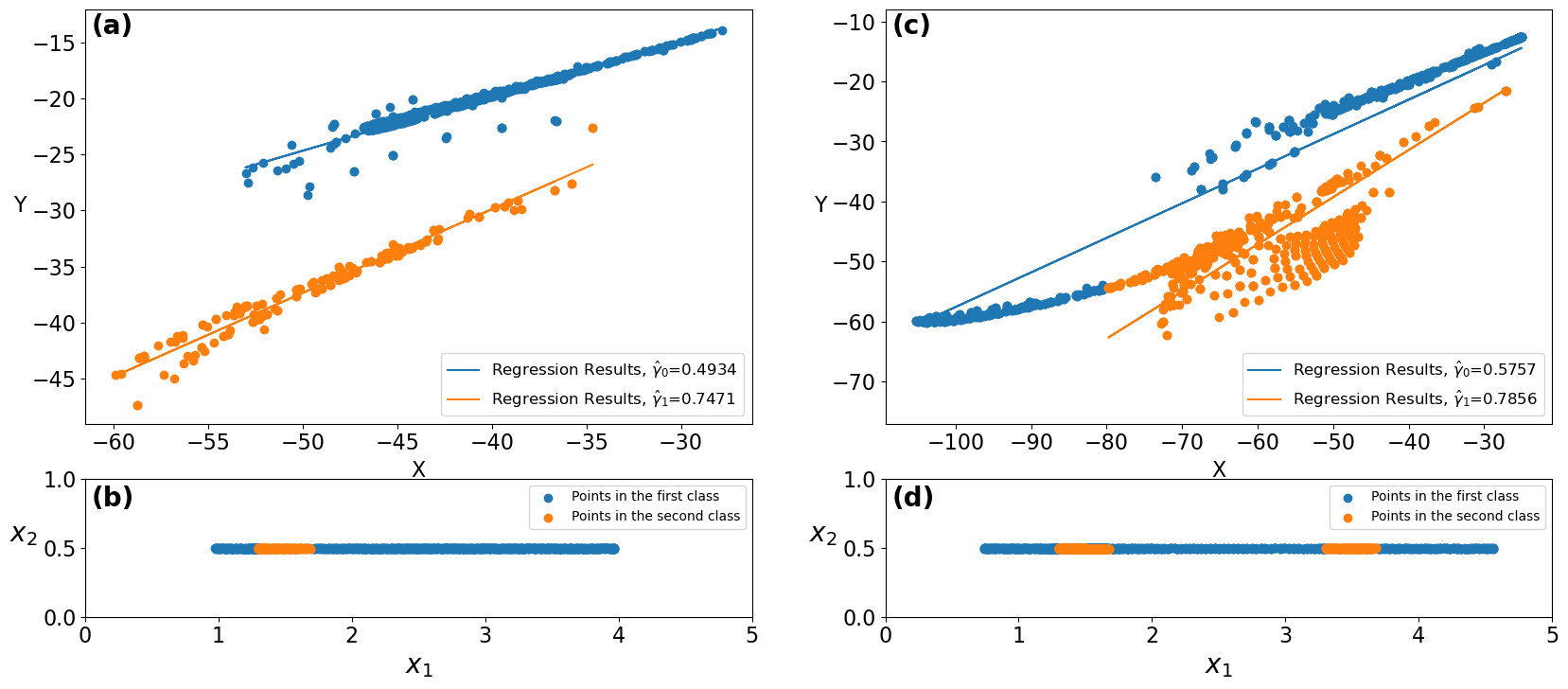
Figure 16: (a) The sampled data in $(X,Y)$ obtained by the $\mathrm{AT_{1}}$ model for the crack propagation in inhomogeneous media with a disk inclusion after the classification using the $k$-means algorithm. The solid line is the result of linear regression for each class. (b) The positions of the data point corresponding to each class. (c) The sampled data in $(X,Y)$ obtained by the $\mathrm{AT_{1}}$ model for the crack propagation in inhomogeneous media with two disk inclusions. The data is classified using the $k$-means algorithm. The solid line is the result of linear regression for each class. (d) The positions of the data point corresponding to each class. The applied strain $A$ in (6) is chosen as $A=1.25$ for (a) and $A=1$ for (c).

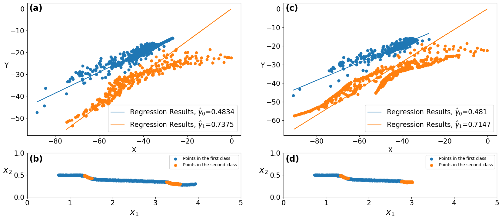
Figure 21: (a) The sampled data in $(X,Y)$ obtained by the $\mathrm{AT_{1}}$ model in the time interval $[80\delta t,480\delta t)$ for the crack propagation in inhomogeneous media with two disk inclusions. The data is classified by using the $k$-means algorithm. The solid line is the result of linear regression for each class. (b) The positions of the data point corresponding to each class. (c) The sampled data in $(X,Y)$ obtained by the $\mathrm{AT_{1}}$ model in the time interval for the crack propagation in inhomogeneous media with two disk inclusions. The data is classified by using the $k$-means algorithm. The solid line is the result of linear regression for each class. (d) The positions of the data point corresponding to each class. The applied strain $A$ in (6) is chosen as $A=1$.

Similar to Sec.4.1.2, we consider the two-disk inclusions. As in Fig. 16(c,d), the estimation is less accurate compared with the $\mathrm{AT_{2}}$ model. Still, we estimate the toughness as $\hat{\gamma}_{1}=0.5757$ and $\hat{\gamma}_{1}=0.7856$, which are reasonably close to the ground truth $\gamma_{0}=0.5$ and $\gamma_{1}=0.75$. Even when the two inclusions are placed at the different $x_{2}$ position (Fig.1(VI,VII)), we may estimate the toughness of the inclusions and their positions (see Fig. 21 in Supplementary Materials). In the $\mathrm{AT_{1}}$ model, because we use the data near the crack tip, the information is limited to the spatial points near the crack path. Therefore, we cannot estimate the whole shape of the inclusions. We may also need data close to the inclusions. This is in contrast with the $\mathrm{AT_{2}}$ model.

5 Discussion

In summary, we study numerical simulations of the crack propagation using the phase-filed models, and propose an algorithm to estimate the fracture toughness as well as the position of the inhomogeneity. The method is based on pre-processing of the data and linear regression. One important step is to sample the grid points at each time in the region where the crack has not arrived to avoid the effect of the plus operator. We successfully demonstrate to estimate the fracture toughness of the inclusion and its position. The method works both for strip and disk inclusions, and both for one- and two-disk inclusions.

In this work, the two different types of energy functional, the $\mathrm{AT_{1}}$ and $\mathrm{AT_{2}}$ models, are studied. Both models exhibit the increase of the $J$-integral corresponding to the inhomogeneous toughness. For the inverse problems, our method works for both models, but the $\mathrm{AT_{1}}$ model requires more pre-processing than the $\mathrm{AT_{2}}$ model. Moreover, the estimation of the position of inclusions is limited for the $\mathrm{AT_{1}}$ model, but not for the $\mathrm{AT_{2}}$ model. This is because the plus operator is effective in a broader region in the $\mathrm{AT_{1}}$ model. In this respect, the $\mathrm{AT_{2}}$ model gives us more information about the inclusions in the inverse problems. Nevertheless, the $\mathrm{AT_{1}}$ model has an advantage that the crack field $z({\bf x},t)$ has a sharper distribution near the crack, and strictly $z=0$ away from the crack. This difference may affect the precision of the computation of the $J$-integral during the crack propagation.

We should note that our method of the estimation of inhomogeneous toughness is based on parameter estimation, and not on model discovery, which is a recent active research field [11]. In the model discovery, a model described by partial differential equations is not a priori known; ideally, elastic equation and phase-field model are estimated from the data. We assume that we know the phase-field model and the linear elastic equation. There are several difficulties in the model discovery in our system. First, we consider slow quasi-static crack propagation, and therefore, $\partial_{t}z\approx 0$. The model discovery based on the regression method relies on minimization of the cost function describing the difference between the left-hand side and right-hand side of the equation with sparse regularization [11]. When the left-hand side ($\partial_{t}z$) vanishes, we cannot uniquely estimate all the coefficients in the right-hand side. Second difficulty is the large parameter contrast in the model of (4) and (5) due to $\epsilon$. The regression with sparse regularization tries to remove a term whose coefficient is small. However, when the model contains a term with larger coefficient $\mathcal{O}(1/\epsilon)$ and one with smaller coefficient $\mathcal{O}(\epsilon)$, it is difficult to keep the $\mathcal{O}(\epsilon)$ term, but remove other unnecessary terms.

For the crack propagation in a homogeneous media, after using the same pre-processing that we use, we may apply the SINDy method, proposed in [11]. If we consider the dictionary terms from the product between $z$ and $u$ and their derivatives: such as $\{u_{x},u_{y},u_{x}^{2},u_{y}^{2},z,z_{x},z_{y},z_{xx},z_{yy},zu_{x},zu_{y},zu_{x}^{2},zu_{y}^{2},zz_{x},zz_{y},zz_{xx},zz_{yy}\}$, we can estimate unnecessary terms particularly when the tolerance is large, (corresponding to weaker sparse regularization). This is due to the large parameter contrast. The first issue mentioned above is not too serious. If we include only the ground-truth terms in the dictionary, our estimation result is

$$z_{t}=0.52447\Delta z-1057.1z-42.221\lvert\nabla u\rvert^{2}+42.350z\lvert\nabla u\rvert^{2},$$ (15)

under the ground-truth parameter $\gamma=0.5$, $\mu=1$, and $\epsilon=0.02$. The estimation does not look working, but the ratio between the first and third terms, and between the second and fourth term in (15) are $\hat{\epsilon}\hat{\gamma}/\hat{\mu}=0.012$ and $\hat{\gamma}/(\hat{\epsilon}\hat{\mu})=24.96$, respectively. Therefore, the estimation works up to constant multiplication.

The application of SINDy for the crack propagation in inhomogeneous media is more involved. Using the same assumption made in our study, namely, if we assume only two values of toughness, we may use the group sparsity [28]. Nevertheless, the difficulties discussed above apply also in the inhomogeneous toughness, and therefore, the estimation of the model is still impractical.

In the original version of SINDy, the estimation is not robust against noise, and accurate computations of spatial and time derivatives are necessary [27]. In our method, we use the Chebyshev polynomial of degree 7. We have tried different interpolation schemes to check how the accuracy of spatial and time derivatives affects the estimation. For example, in the stripe case of the $\mathrm{AT_{2}}$ model, by applying the second-order finite difference method to compute the derivatives of $\widetilde{U}$ and $\widetilde{Z}$, we obtain the estimation $\hat{\gamma}_{0}=0.5015$ and $\hat{\gamma}_{1}=0.75$. The result is shown in Fig. 22 in Supplementary Materials. Even in such a poor evaluation of derivatives, our estimation gives the values close to the ground truth, suggesting that our method does not require very accurate computations of spatial and time derivatives. We speculate this is because we assume we a priori know the model, and therefore, the search space during the optimization is limited.

In our method, we can compute the strain field $\{U_{K}^{n}\}$ in (4) and (5) once the crack field $\{Z_{K}^{n}\}$ is known. This means that we may estimate inhomogeneous toughness only from the information of a crack path. This aspect of the estimation is important because in practical situations, it is difficult to measure a strain field. The strain field should be obtained or estimated from the crack field. However, our method is limited because we assume the linear elastic model and also the elastic constant is known. If these assumptions are not available, we need to estimate the model for the elastic equation, and even for the linear elastic model, we need to estimate the elastic constant. In this case, the estimation only from data of a crack field is more involved. A possible extension of our method is to treat the strain field as a hidden variable, and estimate the inhomogeneous toughness after marginalizing the hidden variable [29].

Appendix A. $k$-means algorithm

In the inhomogeneous case, we used an extension of the classic $k$-means classification to our problem. The algorithm is as follows:

1. We compute the maximum slope and minimum slope of the sample points and denote the values by $a_{max}$ and $a_{min}$ respectively. Then, we choose $\{\gamma_{m}\}_{m=1,2,...k}$ that is $k$ independent random values which follow the uniform distribution $\mathcal{U}(\gamma_{min},\gamma_{max})$;

2. For the sample points $P=\{p_{j}\}$, we define

   $$\operatorname{dist}_{m}(p_{j})=\left[Y(p_{j})-\gamma_{m}X(p_{j})\right]^{2}$$

   and assigned $p_{j}$ to class $\mathrm{arg\,min}_{m=1,2,...k}\operatorname{dist}_{m}(p_{j})$. We assign all the sample points into $k$ classes.

3. In each class, we perform linear regression to update the value of $\{\gamma_{m}\}_{m=1,2,...k}$;

4. We go back to step 2 and reassign the sample points to $k$ classes and then to step 3 to update the values of $\{\gamma_{m}\}_{m=1,2,...k}$. We repeat the algorithm till that $\{\gamma_{m}\}_{m=1,2,...k}$ do not change anymore.

Supplement Material

5.1 Additional data of the estimation of homogeneous material in $\mathrm{AT_{1}}$

5.2 Additional data of the estimation of inhomogeneous toughness

Figure 22: (a) The sampled data in $(X,Y)$ obtained by the $\mathrm{AT_{2}}$ model for the crack propagation in inhomogeneous media with stripe inclusion. The derivatives are computed by the finite difference method. The data is classified by using the $k$-means algorithm. The solid line is the result of linear regression for each class. (b) The positions of the data point corresponding to each class. The applied strain $A$ in (6) is chosen as $A=1.25$.

References

- [1] T.L. Anderson, Fracture Mechanics, Fundamentals and Applications. 4th Edition, Taylor Francis, CRC Press.
- [2] E. Avalos, S. Xie, K. Akagi and Y. Nishiura, Bridging a mesoscopic inhomogeneity to macroscopic performance of amorphous materials in the framework of the phase field modeling. Physica D: Nonlinear Phenomena 409 (2020) 132470. DOI:10.1016/j.physd.2020.132470
- [3] S. Brunton and J. Kutz, Data-Driven Science and Engineering: Machine Learning, Dynamical Systems, and Control. Cambridge: Cambridge University Press. doi:10.1017/9781108380690
- [4] R. Eymard, R. Herbin and T. Gallouët, Discretization of heterogeneous and anisotropic diffusion problems on general nonconforming meshes SUSHI: a scheme using stabilization and hybrid interfaces IMA Journal of Numerical Analysis, Volume 30, Issue 4, October 2010, Pages 1009–1043.
- [5] G.A. Francfort and J.-J. Marigo, Revisiting brittle fracture as an energy minimization problem. Journal of the Mechanics and Physics of Solids 46 (8) (1998) 1319–1342. DOI:10.1016/S0022-5096(98)00034-9
- [6] A.A. Griffith, The phenomena of rupture and flow in solids. Philosophical Transactions of the Royal Society of London. Series A, Containing Papers of a Mathematical or Physical Character, 221 (1921) 163–198. DOI: 10.1098/rsta.1921.0006
- [7] M. Z. Hossain, C.-J. Hsueh, B. Bourdin, and K. Bhattacharya, Effective toughness of heterogeneous media. Journal of the Mechanics and Physics of Solids 71 (2014) 15–32. DOI:10.1016/j.jmps.2014.06.002
- [8] C. Kuhn and R. Müller, A Phase-field model for fracture PAMM Proc. Appl. Math. Mech. 8 (2008) 10223–10224.
- [9] C. Kuhn and R. Müller, A continuum phase field model for fracture Engineering Fracture Mechanics, 77 (2010) 3625–3634.
- [10] M. Lebihain, J.-B. Leblond and L. Ponson, Effective toughness of periodic heterogeneous materials: the effect of out-of-plane excursions of cracks. Journal of the Mechanics and Physics of Solids, 137 (2020) 103876.
- [11] S. H. Rudy, S. L. Brunton, J. L. Proctor and J. N. Kutz, Data-driven discovery of partial differential equations. Sci. Adv. 3, e1602614 (2017).
- [12] E. Tanné, T. Li, B. Bourdin, J.-J. Marigo, C. Maurini Crack nucleation in variational phase-field models of brittle fracture. Journal of the Mechanics and Physics of Solids, Volume 110, January (2018), Pages 80–99.
- [13] T. Takaishi and M. Kimura, Phase field model for mode III crack growth in two-dimensional elasticity, Kybernetika 45 (4) (2009) 605–614.
- [14] J.-Y. Wu, V.-P. Nguyen, C. T. Nguyen, D. Sutula, S. Sinaie and S. Bordas, Chapter One - Phase-field modeling of fracture, Advances in Applied Mechanics, Volume 53, (2020), Pages 1–183.
- [15] M. Ambati, T. Gerasimov, and L. De Lorenzis, A review on phase-field models of brittle fracture and a new fast hybrid formulation, Computational Mechanics, Volume 55, (2015), Pages 383–405.
- [16] M. Ambati, T. Gerasimov, and L. De Lorenzis, Phase-field modeling of ductile fracture , Computational Mechanics, Volume 55, (2015), Pages 1017–1040.
- [17] L. Rozen-Levy, J.M. Kolinski, G. Cohen, and J. Fineberg, How Fast Cracks in Brittle Solids Choose Their Path , Physical Review Letters, Volume 125, (2020), Pages 175501.
- [18] M. Elices, G.V. Guinea, J. Gómez, and J. Planas, The cohesive zone model: advantages, limitations and challenges, Engineering Fracture Mechanics, Volume 69, (2002), Pages 137–163.
- [19] N. Moës, J. Dolbow, and T. Belytschko, A finite element method for crack growth without remeshing, International Journal for Numerical Methods in Engineering, Volume 46, (1999), Pages 131–150.
- [20] B. Bourdin, G. A. Francfort, and J.-J. Marigo, Numerical experiments in revisited brittle fracture, Journal of the Mechanics and Physics of Solids, Volume 48, (2000), Pages 797–826.
- [21] A. Karma, A. E. Lobkovsky, Unsteady crack motion and branching in a phase-field model of brittle fracture, Phys. Rev. Lett. 92 (2004), 245510.
- [22] B. N. J. Persson, E. A. Brener, Crack propagation in viscoelastic solids, Phys. Rev. E 71, (2005), 036123.
- [23] I. S. Aranson, V. A. Kalatsky, V. M. Vinokur, Continuum field description of crack propagation, Phys. Rev. Lett. 85 (2000) 118–121.
- [24] A. Karma, D. A. Kessler, H. Levine, Phase-field model of mode iii dynamic fracture, Phys. Rev. Lett. 87 (2001) 045501.
- [25] V. Hakim, A. Karma, Crack path prediction in anisotropic brittle materials, Phys. Rev. Lett. 95 (2005) 235501.
- [26] M. Bär, R. Hegger, H. Kantz, Fitting partial differential equations to space-time dynamics, Phys. Rev. E 59 (1999) 337–342.
- [27] H. Schaeffer, S. G. McCalla, Sparse model selection via integral terms, Phys. Rev. E 96 (2017) 023302.
- [28] S. Rudy, A. Alla, S. Brunton, and J.N. Kutz, Data-driven identification of parametric partial differential, arXiv:1806.00732 (2018).
- [29] C.M. Bishop, Pattern recognition and machine learning, Springer New York.