Quantum speed limit of a noisy continuous-variable system

Abstract

Setting the minimal-time bound for a quantum system to evolve between two distinguishable states, the quantum speed limit (QSL) characterizes the latent capability in speeding up of the system. It has found applications in determining the quantum superiority in many quantum technologies. However, previous results showed that such a speedup capability is generally destroyed by the environment induced decoherence in the Born-Markovian approximate dynamics. We here propose a scheme to recover the speedup capability in a dissipative continuous-variable system within the exact non-Markovian framework. It is found that the formation of a bound state in the energy spectrum of the total system consisting of the system and its environment can be used to restore the QSL to its noiseless performance. Giving an intrinsic mechanism in preserving the QSL, our scheme supplies a guideline to speed up certain quantum tasks in practical continuous-variable systems.

I Introduction

The quantum speed limit (QSL) quantifies the maximal speed at which a quantum system evolves under the constraint of quantum mechanics. Mandelstam and Tamm showed that, for a unitary dynamics governed by a Hamiltonian $\hat{H}$, the minimal evolution time between two orthogonal states is $\tau_{\text{MT}}=\pi\hbar/(2\Delta H)$ with $(\Delta H)^{2}\equiv\langle\hat{H}^{2}\rangle-\langle\hat{H}\rangle^{2}$ being the energy fluctuation Mandelstam and Tamm (1945); Anandan and Aharonov (1990). This result provides a physical explanation to Heisenberg’s energy-time uncertainty relation Mandelstam and Tamm (1945); Gislason et al. (1985); Boykin et al. (2007); Deffner and Campbell (2017). Later, Margolus and Levitin provided an alternative QSL time in terms of the energy difference $\tau_{\text{ML}}=\pi\hbar/(2\langle\hat{H}\rangle)$ Margolus and Levitin (1998); Jones and Kok (2010). Sun and Zheng derived a distinct QSL bound via the gauge invariant distance Sun and Zheng (2019). The above three independent bounds are summarized in a unified form for both Hermitian and non-Hermitian quantum systems Sun et al. (2021).

Recently, much effort has been devoted to generalizing the concept of QSL from closed systems to open systems Deffner and Lutz (2013); Taddei et al. (2013); del Campo et al. (2013); Marvian and Lidar (2015); Van Vu and Hasegawa (2021); Funo et al. (2019). Deffner and Lutz derived a Margolus-Levitin-type bound on the minimal evolution time of open quantum systems Deffner and Lutz (2013). A generalized geometric interpretation for the Margolus-Levitin-like QSL was provided by Ref. Pires et al. (2016). From the application perspective, the QSL in open quantum systems is closely related to the greatest efficiency of charging power in quantum batteries Campaioli et al. (2017); Santos et al. (2019); García-Pintos et al. (2020), the minimum operation time of quantum gates Ashhab et al. (2012); Negîrneac et al. (2021), the entropy production rate of nonequilibrium quantum thermodynamics Deffner and Lutz (2010); Plastina et al. (2014); Mancino et al. (2018); Shiraishi et al. (2018); Nicholson et al. (2020); Lam et al. (2021), as well as the quantum Fisher information in noisy quantum metrology Giovannetti et al. (2011); Alipour et al. (2014); Pires et al. (2016); Beau and del Campo (2017); Falasco and Esposito (2020); Ito and Dechant (2020). Thus, how to establish a unified QSL bound, which is valid for both unitary and nonunitary evolutions, is of importance. Using the information geometric formalism is a possible solution Pires et al. (2016); Sun and Zheng (2019); Sun et al. (2021); Deffner and Campbell (2017); Shanahan et al. (2018); Deffner (2017). Starting from a geometric perspective, Refs. Campaioli et al. (2018, 2019) reported QSL bounds, which outperform the traditional bounds for both closed and open systems. As already shown in Refs. Sun and Zheng (2019); Sun et al. (2021); Liu et al. (2016), the QSL can be used to quantify the potential capability of speeding up for quantum systems. Such a speedup potency plays a leading role in quantum control Deffner and Campbell (2017); Aifer and Deffner (2022).

However, due to the decoherence induced by the inevitable system-environment interaction, the potency of quantum speedup generally vanishes in the Born-Markovian approximate decoherence dynamics  Taddei et al. (2013); del Campo et al. (2013); Marvian and Lidar (2015); Van Vu and Hasegawa (2021); Liu et al. (2016); Hu et al. (2020); Marian and Marian (2021); Xu et al. (2019); Xu (2016). How to preserve such a capacity is of importance in the protocol of quantum technology and quantum control. On the other hand, most of the existing studies of the QSL in open quantum systems have focused on the discrete-variable case Deffner and Lutz (2013); Taddei et al. (2013); del Campo et al. (2013); Marvian and Lidar (2015); Van Vu and Hasegawa (2021); Liu et al. (2016); Xu et al. (2019); Xu (2016); Wu and An . Very few studies concentrate on the continuous-variable case, especially in the non-Markovian dynamics. In this paper, we investigate the QSL in a dissipative continuous-variable system beyond the traditional paradigm of Born-Markovian approximation treatment. A bound-state based mechanism to realize a controllable QSL time in the noisy environment is revealed.

The paper is organized as follows. The QSL for a Gaussian continuous-variable system being applicable in both the closed and open systems is derived in Sec. II. The non-Markovian decoherence effect on the QSL time is investigated in Sec. III. A mechanism to recover the ideal speedup capacity of the continuous-variable system under the non-Markovian noise is uncovered. In Sec. IV, we make a comparison of our scheme with the previous characterization schemes to the QSL in order to exhibit the universality of our result. Finally, a discussion and a summary are made in Sec. V.

II QSL in a Gaussian system

The QSL can be obtained from the viewpoint of the information geometry as follows. By introducing any kind of geodesic measure $\mathcal{L}=\mathcal{L}(\varrho_{\tau},\varrho_{0})$ quantifying the lower distance bound between two quantum states $\varrho_{\tau}$ and $\varrho_{0}$, an inequality is accordingly built as $\mathcal{L}\leq\ell\equiv\int\sqrt{d\ell^{2}}$. Here, $d\ell^{2}$ denotes the squared infinitesimal length between $\varrho_{\tau}$ and $\varrho_{\tau}+d\varrho_{\tau}$, which is regarded as the metric Provost and Vallee (1980); Funo et al. (2019), and thus $\ell$ is the length of the actual evolution path. Via introducing the time-averaged evolution speed $\bar{v}=\ell/\tau$, the QSL time is geometrically described as $\tau_{\mathrm{QSL}}\equiv\mathcal{L}/\bar{v}$, which implies $\tau_{\mathrm{QSL}}/\tau=\mathcal{L}/\ell$ Pires et al. (2016); Deffner and Campbell (2017); Funo et al. (2019). This result indicates that $\tau_{\mathrm{QSL}}/\tau$ characterizes the extent of the actual evolution path deviating from the geodesic path Sun and Zheng (2019); Sun et al. (2021); Liu et al. (2016). If $\tau_{\text{QSL}}/\tau=1$, the length of the actual evolution path saturates the geodesic one and there is no more space for speeding up. In contrary, the quantum system has a potential speedup capacity as long as $\tau_{\text{QSL}}/\tau<1$. The smaller the value of $\tau_{\mathrm{QSL}}/\tau$ is, the more speedup capability the system may possess. Therefore, $\tau_{\text{QSL}}/\tau$ is physically a characterization of the latent capability in speeding up of the quantum system. It has been found that such a capability has important applications in quantum technologies Campaioli et al. (2017); Santos et al. (2019); García-Pintos et al. (2020); Ashhab et al. (2012); Negîrneac et al. (2021); Deffner and Campbell (2017); Aifer and Deffner (2022). It should be emphasized that the QSL bound considered in our paper is completely different from the so-called quantum brachistochrone problem Carlini et al. (2006); Frydryszak and Tkachuk (2008); Hegerfeldt (2013). The quantum brachistochrone problem commonly aims at designing an optimally controlled time-dependent Hamiltonian such that the shortest evolution time from a given initial state to a final one is achieved under a set of given constraints. It belongs to the research field of quantum optimal control. In this paper, we concentrate on an autonomous time-independent open system.

The Bures angle Jozsa (1994); Deffner and Campbell (2017); Taddei et al. (2013)

$$\mathcal{L}_{\text{B}}\equiv\text{arccos}\text{Tr}\bigg{(}\sqrt{\sqrt{\varrho_{0}}\varrho_{\tau}\sqrt{\varrho_{0}}}\bigg{)},$$ (1)

is widely used to measure the geodesic length between $\varrho_{0}$ and $\varrho_{\tau}$. The corresponding metric known as the so-called Fisher-Rao metric relates to the famous quantum Fisher information as $d\ell^{2}=\frac{1}{4}\mathcal{F}_{\text{Q}}dt^{2}$  Pires et al. (2016); Deffner and Campbell (2017); Taddei et al. (2013); Braunstein and Caves (1994). Here, the quantum Fisher information $\mathcal{F}_{\text{Q}}$ is defined by $\mathcal{F}_{\text{Q}}=\text{Tr}(\varrho_{t}\hat{L}^{2})$ with $\hat{L}$ determined by $\dot{\varrho}_{t}=(\hat{L}\varrho_{t}+\varrho_{t}\hat{L})/2$. Then, the averaged speed $\bar{v}$ and the QSL time $\tau_{\mathrm{QSL}}$ are derived as Pires et al. (2016); Deffner and Campbell (2017); Taddei et al. (2013); O’Connor et al. (2021); Hörnedal et al. (2022)

$$\bar{v} = \frac{1}{2\tau}\int_{0}^{\tau}dt\sqrt{\mathcal{F}_{\text{Q}}},$$ (2)

$$\tau_{\mathrm{QSL}} = \frac{\mathcal{L}_{\text{B}}}{\bar{v}}=\frac{\mathcal{L}_{\text{B}}}{\ell}\tau.$$ (3)

It is found that $\mathcal{L}_{\text{B}}$ and $\mathcal{F}_{\text{Q}}$ naturally reduce to $\pi/2$ and $4(\langle\psi|\hat{H}^{2}|\psi\rangle-\langle\psi|\hat{H}|\psi\rangle^{2})$, respectively, in the special case of the pure states under the unitary evolution, i.e., $\varrho_{0}=|\psi\rangle\langle\psi|$ and $\varrho_{\tau}=|\psi_{\perp}\rangle\langle\psi_{\perp}|$ with $\langle\psi|\psi_{\perp}\rangle=0$. Then, $\tau_{\text{QSL}}$ recovers the well-known Mandelstam-Tamm bound.

Here, we consider a single-mode continuous-variable system consisting of a pair of annihilation and creation operators $\hat{A}=\{\hat{a},\hat{a}^{\dagger}\}$. The characteristic function of the system is defined as $\chi(\boldsymbol{\xi})\equiv\text{Tr}[\varrho_{t}\mathcal{\hat{D}}(\boldsymbol{\xi})]$ Braunstein and van Loock (2005); Šafránek et al. (2015), where $\mathcal{\hat{D}}(\boldsymbol{\xi})=\exp(\hat{A}^{\dagger}K\boldsymbol{\xi})$, with $K=\text{Diag}(1,-1)$ and $\boldsymbol{\xi}=(\xi,\xi^{*})^{\text{T}}$, is the Weyl displacement operator. If the characteristic function has a Gaussian form $\chi(\boldsymbol{\xi})=\exp(-\frac{1}{4}\boldsymbol{\xi}^{\dagger}\boldsymbol{\sigma}\boldsymbol{\xi}-i\boldsymbol{d}^{\dagger}K\boldsymbol{\xi})$, then such a continuous-variable system is called a Gaussian system. Its characteristic function is fully determined by the displacement vector $\boldsymbol{d}_{t}$ with $d_{t}^{j}=\text{Tr}(\varrho_{t}\hat{A}_{j})$ and the covariance matrix $\boldsymbol{\sigma}_{t}$ with $\sigma_{t}^{ij}=\text{Tr}(\varrho_{t}\{\hat{A}_{i}-d_{i},\hat{A}^{\dagger}_{j}-d^{*}_{j}\})$. For a Gaussian continuous-variable system, the Bures angle reads $\mathcal{L}_{\text{B}}=\text{arccos}\sqrt{F}$. Here, $F$ is the quantum fidelity and is calculated by using the displacement vectors and the covariance matrices as Scutaru (1998); Šafránek et al. (2015); Marian and Marian (2012)

$$F=\frac{2\exp[-(\boldsymbol{d}_{0}-\boldsymbol{d}_{t})^{\dagger}(\boldsymbol{\sigma}_{0}+\boldsymbol{\sigma}_{t})^{-1}(\boldsymbol{d}_{0}-\boldsymbol{d}_{t})]}{\sqrt{\Gamma}+\sqrt{\Lambda}-\sqrt{(\sqrt{\Gamma}+\sqrt{\Lambda})^{2}-\Pi}},$$ (4)

where $\Pi=\text{Det}(\boldsymbol{\sigma}_{0}+\boldsymbol{\sigma}_{t})$, $\Gamma=\text{Det}(\mathbf{1}+K\boldsymbol{\sigma}_{0}K\boldsymbol{\sigma}_{t})$, and $\Lambda=\text{Det}(\boldsymbol{\sigma}_{0}+K)\text{Det}(\boldsymbol{\sigma}_{t}+K)$. On the other hand, the quantum Fisher information with respect to the evolution time for a Gaussian system is calculated by Šafránek (2018)

$$\mathcal{F}_{\text{Q}}=\frac{1}{2}\text{Vec}[\dot{\boldsymbol{\sigma}}_{t}]^{\dagger}M^{-1}\text{Vec}[\dot{\boldsymbol{\sigma}}_{t}]+2\dot{\boldsymbol{d}}_{t}^{\dagger}\boldsymbol{\sigma}^{-1}_{t}\dot{\boldsymbol{d}}_{t},$$ (5)

where $\text{Vec}[\cdot]$ denotes the vectorization of a given matrix and $M=\boldsymbol{\sigma}_{t}^{*}\otimes\boldsymbol{\sigma}_{t}-K\otimes K$. From these results, as long as $\boldsymbol{d}_{t}$ and $\boldsymbol{\sigma}_{t}$ are known, the QSL in a Gaussian continuous-variable system is fully determined.

Let us first consider the QSL of a quantum harmonic oscillator in the ideal case of a unitary evolution governed by $\hat{H}_{\text{s}}=\omega_{0}\hat{a}^{\dagger}\hat{a}$. The initial state is chosen as a coherent state, namely, $\varrho_{\text{s}}(0)=\mathcal{\hat{D}}(\alpha)|0\rangle\langle 0|\mathcal{\hat{D}}(\alpha)^{\dagger}$. It is readily derived that $\boldsymbol{d}_{t}=(\alpha e^{-i\omega_{0}t},\alpha^{*}e^{i\omega_{0}t})^{\text{T}}$ and $\boldsymbol{\sigma}_{t}=\mathbf{1}$, which lead to $F=e^{-2|\alpha|^{2}[1-\cos(\omega_{0}\tau)]}$ and $\mathcal{F}_{\text{Q}}=4|\alpha|^{2}\omega_{0}^{2}$. Thus, we have $\bar{v}=|\alpha|\omega_{0}$, which is a time-independent constant, and thus

$${\tau_{\mathrm{QSL}}\over\tau}=\frac{\arccos e^{-|\alpha|^{2}[1-\cos(\omega_{0}\tau)]}}{|\alpha|\omega_{0}\tau}.$$ (6)

Equation (6) reveals that the QSL time behaves as $\tau_{\mathrm{QSL}}/\tau\propto\tau^{-1}$ with the actual evolution time $\tau$. It means $\tau_{\mathrm{QSL}}/\tau$ approaches to zero in the large-$\tau$ regime. Such a result implies that the harmonic oscillator has an infinite speedup capability in this noiseless case.

III QSL in a noisy environment

Next, we consider a more practical situation in which the harmonic oscillator is coupled to a dissipative bosonic environment and experiences a decoherence. The Hamiltonian of the total system reads

$$\begin{split}\hat{H}=&\hat{H}_{\text{s}}+\sum_{k}\omega_{k}\hat{b}_{k}^{\dagger}\hat{b}_{k}+\sum_{k}\Big{(}g_{k}\hat{a}^{\dagger}\hat{b}_{k}+\mathrm{H}.\mathrm{c}.\Big{)},\end{split}$$ (7)

where $\hat{b}_{k}$ denotes the annihilation operator of the $k$th environmental mode with frequency $\omega_{k}$, and the parameter $g_{k}$ is the coupling strength between the harmonic oscillator and the $k$th environmental mode. The coupling strength is further characterized by the spectral density $J(\omega)\equiv\sum_{k}|g_{k}|^{2}\delta(\omega-\omega_{k})$. We consider that $J(\omega)$ explicitly takes the following Ohmic-family form:

$$J(\omega)=\eta\omega^{s}\omega_{c}^{1-s}e^{-\omega/\omega_{c}},$$ (8)

where $\eta$ is a dimensionless coupling constant, $\omega_{c}$ is a cutoff frequency, and $s$ is the so-called Ohmicity parameter. Depending on the value of $s$, the environment can be classified into the sub-Ohmic for $0<s<1$, the Ohmic for $s=1$, and the super-Ohmic for $s>1$.

Considering the environment is initially prepared in its vacuum state and using Feynman-Vernon’s influence functional method to partially trace out the degrees of freedom of the dissipative environment, we obtain an exact non-Markovian master equation for the harmonic oscillator as An and Zhang (2007); Yang et al. (2014); Wu et al. (2021)

$$\dot{\varrho}_{t}=-i\big{[}\Omega(t)\hat{a}^{\dagger}\hat{a},\varrho_{t}\big{]}+\gamma(t)\Big{(}2\hat{a}\varrho_{t}\hat{a}^{\dagger}-\{\hat{a}^{\dagger}\hat{a},\varrho_{t}\}\Big{)},$$ (9)

where $\Omega(t)=-\text{Im}[\dot{u}(t)/u(t)]$ is the renormalized frequency and $\gamma(t)=-\text{Re}[\dot{u}(t)/u(t)]$ is the decay rate induced by the dissipative environment. The time-dependent coefficient $u(t)$ is determined by

$$\dot{u}(t)+i\omega_{0}u(t)+\int_{0}^{t}d\tau\mu(t-\tau)u(\tau)=0,$$ (10)

with $u(0)=1$ and $\mu(t)\equiv\int_{0}^{\infty}d\omega J(\omega)e^{-i\omega t}$.

In order to compare with that of the noiseless ideal case, we still choose that the quantum harmonic oscillator is initially in a coherent state. Then, solving the master equation (9), we calculate the exact expressions of the displacement vector and the covariance matrix as $\boldsymbol{d}_{t}=[\alpha u(t),\alpha^{*}u(t)^{*}]^{\mathrm{T}}$ and $\boldsymbol{\sigma}_{t}=\mathbf{1}$. With the above expressions at hand, the time-averaged speed $\bar{v}$ and the geodesic distance $\mathcal{L}_{\text{B}}$ in the noise case are straightforwardly computed:

$$\bar{v} = \frac{1}{\tau}\int_{0}^{\tau}dt|\alpha\dot{u}(t)|,$$ (11)

$$\mathcal{L}_{\text{B}} = \arccos\sqrt{e^{-|\alpha[1-u(\tau)]|^{2}}}.$$ (12)

We consider the QSL of the system relaxing to its steady state by choosing $\tau$ sufficiently large. The QSL time derived under such a condition reflects the equilibration efficiency of the dissipative harmonic oscillator. The controllability of this equilibration efficiency is vital in suppressing the detrimental effect of the decoherence in practical quantum technologies.

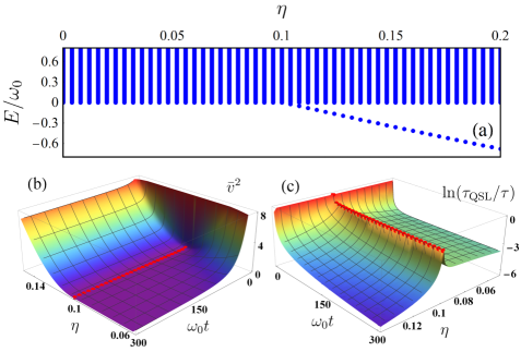
Figure 1: (a) Energy spectrum of $\hat{H}$ in the single-excitation subspace. Exact non-Markovian result of the average speed (b) and the QSL time (c) with different $\eta$ and $\omega_{0}t$. The red circles highlight the positions of the threshold coupling strength $\eta=0.1$ at which the bound state occurs. Other parameters are $|\alpha|=10$, $s=1$, and $\omega_{c}=10\omega_{0}$.

If the system-environment coupling is weak and the characteristic time scale of the environmental correlation function is much smaller than that of the system, one can safely apply the Born-Markovian approximation to Eq. (10). Under such a circumstance, one calculates Yang et al. (2014); Wu et al. (2021) $u^{\text{MA}}(t)\simeq e^{-\{\kappa+i[\omega_{0}+\Delta(\omega_{0})]\}t}$, where $\kappa=\pi J(\omega_{0})$ is the Markovian decay coefficient and $\Delta(\omega_{0})=\mathcal{P}\int_{0}^{\infty}d\omega{J(\omega)\over\omega_{0}-\omega}$ is the environmentally induced frequency shift. With the approximate expression of $u^{\text{MA}}(t)$ at hand, we find, under the Born-Markovian approximation, $\bar{v}=|\alpha|\sqrt{\kappa^{2}+\omega_{0}^{2}}(1-e^{-\kappa\tau})/(\kappa\tau)$ and

$$\lim_{\tau\rightarrow\infty}\frac{\tau_{\mathrm{QSL}}}{\tau}=\frac{\kappa\arccos e^{-\frac{1}{2}|\alpha|^{2}}}{|\alpha|\sqrt{\kappa^{2}+\omega_{0}^{2}}},$$ (13)

where we have dropped the contributions from the frequency shift term $\Delta(\omega_{0})$. Equation (13) reduces to the one of the noiseless case in the limit $\kappa\rightarrow 0$. We here choose a large $\tau$, which means we focus on the QSL time from the initial coherent state to the equilibrium state. In this limit, we find that $\bar{v}$ reduces to zero and $\tau_{\mathrm{QSL}}/\tau$ evolves to a time-independent value. This result implies that the speedup potency of the system is destroyed by the Born-Markovian decoherence. A similar result was also reported in several previous references Hu et al. (2020); Marian and Marian (2021); Deffner (2017); Poggi et al. (2021).

Going beyond the Born-Markovian approximation, the results of $\bar{v}$ and $\tau_{\text{QSL}}/\tau$ are obtainable by numerically solving Eq. (10). However, via analyzing the long-time behavior of $u(\tau)$, we calculate their analytically asymptotic forms in the limit $\tau\rightarrow\infty$, which shall help us to build up a more clear physical picture on our results. To this aim, we apply a Laplace transform to $u(\tau)$ and find $\tilde{u}(z)\equiv\int_{0}^{\infty}d\tau u(\tau)e^{-z\tau}=[z+i\omega_{0}+\int_{0}^{\infty}d\omega{J(\omega)\over z+i\omega}]^{-1}$. The solution of $u(\tau)$ is immediately obtained by applying an inverse Laplace transform to $\tilde{u}(z)$, which is exactly done by finding the poles of $\tilde{u}(z)$ from the following transcendental equation:

$$y(\varpi)\equiv\omega_{0}-\int_{0}^{\infty}d\omega{J(\omega)\over\omega-\varpi}=\varpi,$$ (14)

with $\varpi=iz$. It is necessary to point out that the root of the above equation is just the eigenenergy of $\hat{H}$ in the single-excitation subspace. To be more specific, we express the single-excitation eigenstate as $|\Psi\rangle=(x\hat{a}^{\dagger}+\sum_{k}y_{k}\hat{b}_{k}^{\dagger})|0,\{0_{k}\}\rangle$. Substituting it into $\hat{H}|\Psi\rangle=E|\Psi\rangle$, one finds the energy eigen-equation as $E-\omega_{0}-\sum_{k}g_{k}^{2}/(\omega_{k}-E)=0$, which retrieves Eq. (14) via simply replacing $E$ by $\varpi$. This result implies that, although the subspaces with arbitrary excitation number are involved in the reduced dynamics, the dynamics of $u(\tau)$ is essentially determined by the single-excitation energy spectrum characteristic of $\hat{H}$. Because $y(\varpi)$ is a monotonically decreasing function in the regime $\varpi<0$, Eq. (14) potentially has one isolated root $E_{b}$ in this regime provided $y(0)<0$. While $y(\varpi)$ is not well analytic in the regime $\varpi>0$, Eq. (14) has infinite roots in this regime and forms a continuous energy band. We call the eigenstate corresponding to the isolated eigenenergy $E_{b}$ the bound state. Then, after applying the inverse Laplace transform and using the residue theorem, we obtain Yang et al. (2014); Wu et al. (2021)

$$u(\tau)=Ze^{-iE_{b}\tau}+\int_{0}^{\infty}\frac{J(\omega)e^{-i\omega\tau}d\omega}{[\omega-\omega_{0}-\Delta(\omega)]^{2}+[2\pi J(\omega)]^{2}},$$

where the first term with $Z\equiv[1+\int_{0}^{\infty}{J(\omega)d\omega\over(E_{b}-\omega)^{2}}]^{-1}$ is contributed from the potentially formed bound state energy $E_{b}$, and the second term is from the band energy which approaches to zero in the long-time regime due to out-of-phase interference. Thus, if the bound state is absent, then we have $u(\infty)=0$, which leads to a complete decoherence; while if the bound state with energy $E_{b}$ is formed, then we have $u(\infty)\simeq Ze^{-iE_{b}\tau}$, which implies a dissipationless dynamics. The condition of forming the bound state for the Ohmic-family spectral density is evaluated via $y(0)<0$ as $\omega_{0}-\eta\omega_{c}\Gamma(s)<0$, where $\Gamma(s)$ is Euler’s gamma function.

In the absence of the bound state, it is natural to expect a consistent result with that under the Born-Markovian approximation because $u(\tau)$ approaches zero eventually. In contrary, with the long-time expression of $u(\infty)\simeq Ze^{-iE_{b}\tau}$ in the presence of the bound state, we find $\bar{v}\simeq|\alpha ZE_{b}|$ and

$$\frac{\tau_{\mathrm{QSL}}}{\tau}=\frac{\arccos e^{-\frac{1}{2}|\alpha|^{2}[1+Z^{2}-2Z\cos(E_{b}\tau)]}}{|\alpha ZE_{b}|\tau}.$$ (15)

We see from Eq. (15) that, in the limit $\tau\rightarrow\infty$, $\bar{v}$ approaches to a non-zero value, while $\tau_{\mathrm{QSL}}/\tau$ reduces to zero in the form of $\tau^{-1}$. These results are verified by exact numerical simulations (see Fig. 1) and are completely different from those under the Born-Markovian case Hu et al. (2020); Marian and Marian (2021); Deffner (2017). Compared to that of the noiseless ideal case, recovering the relation $\tau_{\mathrm{QSL}}/\tau\propto\tau^{-1}$ means the potency of quantum speedup is fully retrieved. In Fig. 2, we plot the long-time steady-state $\bar{v}$ and $\tau_{\text{QSL}}/\tau$ as functions of $\eta$ and $\omega_{c}/\omega_{0}$. It confirms that there exists a threshold from no-speedup to speedup regimes matching well with the position of forming the bound state. Our result implies that the time-averaged quantum speed and the QSL time are controllable via engineering the energy spectrum of the whole oscillator-environment system.

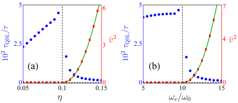
Figure 2: (a) Steady-state average speed (red rectangles) and QSL time (blue circles) as a function of $\eta$ (a) and $\omega_{c}/\omega_{0}$ (b) when $\omega_{0}\tau=400$. The green solid lines are obtained from the analytical result $\bar{v}^{2}\simeq|\alpha|^{2}Z^{2}E_{b}^{2}$. Other parameters are chosen as $|\alpha|=10$ and $s=1$.

IV Comparisons with previous studies

In several previous articles Hu et al. (2020); Marian and Marian (2021); Deffner (2017), the Wigner function and the Wasserstein distance are used to calculate the QSL time in Gaussian continuous-variable systems. As displayed in Refs. Hu et al. (2020); Marian and Marian (2021); Deffner (2017), within the framework of the Wigner representation, the geodesic length between two Wigner distributions, $W_{\tau}(\boldsymbol{\zeta})$ and $W_{0}(\boldsymbol{\zeta})$ with $\boldsymbol{\zeta}=(x,p)^{\text{T}}=(\frac{\xi+\xi^{*}}{\sqrt{2}},\frac{\xi-\xi^{*}}{\sqrt{2}i})^{\text{T}}$ being the quadrature vector, is quantified by using the Wasserstein-$2$ distance as

$$\begin{split}\mathcal{L}_{W}=&\|W_{\tau}(\boldsymbol{\zeta})-W_{0}(\boldsymbol{\zeta})\|_{2}\\ \equiv&\big{\{}\int d\boldsymbol{\zeta}|W_{\tau}(\boldsymbol{\zeta})-W_{0}(\boldsymbol{\zeta})|^{2}\big{\}}^{\frac{1}{2}}.\end{split}$$ (16)

Then the averaged evolution speed $\bar{v}_{W}$ and the QSL time $\tau^{W}_{\mathrm{QSL}}$ in the Wigner space are established as Deffner (2017)

$$\bar{v}_{W} = \frac{1}{\tau}\int_{0}^{\tau}dt\|\dot{W}_{t}(\boldsymbol{\zeta})\|_{2},$$ (17)

$$\tau^{W}_{\mathrm{QSL}} = \frac{\mathcal{L}_{W}}{\bar{v}_{W}}.$$ (18)

The above formalism was further generalized to the Wasserstein-$p$-distance cases with $p=1,2$ and $+\infty$, but computing these Wasserstein distances is rather complicated Deffner (2017).

For our dissipative harmonic oscillator system, the exact expression of the Wigner function is given by Chen et al. (2019); Wu et al. (2021)

$$W_{t}(\boldsymbol{\zeta})=\frac{e^{-\frac{1}{2}(\boldsymbol{\zeta}-\tilde{\boldsymbol{d}}_{t})^{\mathrm{T}}\tilde{\boldsymbol{\sigma}}_{t}^{-1}(\boldsymbol{\zeta}-\tilde{\boldsymbol{d}}_{t})}}{\pi\sqrt{|\mathrm{Det}\tilde{\boldsymbol{\sigma}}_{t}|}},$$ (19)

where $\tilde{\boldsymbol{d}}_{t}=(\sqrt{2}\text{Re}[\alpha u(t)],\sqrt{2}\text{Im}[\alpha u(t)])^{\text{T}}$ and $\tilde{\boldsymbol{\sigma}}_{t}=\frac{1}{2}\boldsymbol{\sigma}_{t}$. With the above expression at hand, we find

$$\bar{v}_{W} = \frac{2}{\sqrt{\pi}\tau}\int_{0}^{\tau}dt|\alpha\dot{u}(t)|,$$ (20)

$$\mathcal{L}_{W} = \frac{2}{\sqrt{\pi}}\big{\{}1-e^{-2|\alpha|^{2}([\text{Re}u(\tau)-1]^{2}+[\text{Im}u(\tau)-1]^{2})}\big{\}}^{\frac{1}{2}}.$$ (21)

It is immediately observed that Eq. (20) matches Eq. (11) except for a trivial pre-factor $2/\sqrt{\pi}$. Moreover, in the limit $\tau\rightarrow\infty$, we find that $\tau_{\text{QSL}}^{W}/\tau$ approaches to a non-zero constant in the absence of the bound state, and $\tau_{\text{QSL}}^{W}/\tau\propto\tau^{-1}$ in the presence of the bound state (see Fig. 3). This conclusion is completely consistent with that of $\tau_{\text{QSL}}$ obtained in Sec. III. It demonstrates that our bound-state-based QSL-controlling scheme is universal to different definitions of QSL time.

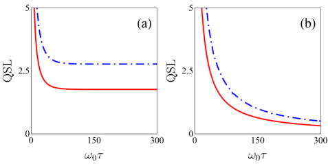
Figure 3: (a) The QSL time $10^{2}\tau_{\text{QSL}}/\tau$ (blue dot-dashed line) and $10^{2}\tau^{W}_{\text{QSL}}/\tau$ (red solid line) are plotted as a function of $\omega_{0}\tau$ in the absence of a bound state when $\eta=0.06$. (b) The same as (a), but in the presence of a bound state with $\eta=0.12$. Other parameters are chosen as $|\alpha|=10$ and $s=1$.

Next, we compare the tightness of $\tau_{\text{QSL}}$ and $\tau_{\text{QSL}}^{W}$. Based on our numerical simulations, $\tau_{\text{QSL}}$ is not always tighter than $\tau_{\text{QSL}}^{W}$ during the whole relaxation process. However, as displayed in Fig. 3, the value of $\tau_{\text{QSL}}$ is larger than $\tau_{\text{QSL}}^{W}$ in the large-$\tau$ regime irrespective of whether the bound state is formed or not. These results mean that the QSL considered in this paper can be tighter than the previous one derived by using the Wigner function and Wasserstein-2 distance. Furthermore, it is noted that, although both our paper and the ones in Refs. Hu et al. (2020); Marian and Marian (2021); Deffner (2017) provide a computable way to obtain the QSL time in Gaussian continuous-variable systems, the QSL formulation in our paper is strictly established in the differential geometry, which is more rigorous in the mathematical sense. In fact, the Fisher-Rao metric employed by us is a contractive Riemannian metric on the set of density operators. As discussed in Ref. Pires et al. (2016), such a peculiar mathematical property may help us to find the tightest bound on the QSL time.

V Discussion and Summary

It is necessary to emphasize that our bound-state based QSL-controlling scheme is independent of the choice of the spectral density. Although only the Ohmic-family form is considered in this paper, our result is straightforwardly generalizable to other cases without difficulties. The bound-state effect, which generally appears in the non-Markovian regime, is the crucial ingredient in our scheme of achieving a steerable QSL. How to generate the bound state is the main point in realizing our control scheme from an experimental perspective. Fortunately, thanks to the rapid development in the state-of-the-art technique of quantum optics experiments, the bound state and its dynamical effect have been observed in circuit quantum electrodynamics architecture Liu and Houck (2017) and matter-wave systems Krinner et al. (2018). With the help of the reservoir engineering technique, the primary parameters in the spectral density $J(\omega)$ are experimentally controllable. The spectral density of a quantum emitter acting as an open system coupling to the surface-plasmon polariton as an environment is adjustable by changing the distance between them Andersen et al. (2011); Yang and An (2017). For a reservoir consisting of ultracold atomic gas, the Ohmicity parameter $s$ is tunable from the sub-Ohmic to the super-Ohmic forms by increasing the scattering length of the gas via Feshbach resonances Haikka et al. (2011). These experimental achievements provide a strong support to our theoretical investigations. As a final remark, our present paper is completely different from Ref. Wu and An . We here investigate the QSL time derived by the Fisher-Rao metric of a continuous-variable system. However, Ref. Wu and An considered the Fubini-Study-metric-based QSL of a dissipative two-level system. From the technical point of view, we need an exact expression of the deterministic quantum master equation to obtain the QSL. In contrast, Ref. Wu and An proposed a scheme to calculate the QSL time via solving the stochastic Schrödinger equation governed by an effective non-Hermitian Hamiltonian. Thus, neither the conclusions nor the methodology of Ref. Wu and An is directly applicable to our present paper.

In summary, by making use of an exact non-Markovian treatment, we investigate the time-averaged evolution speed and the QSL time in an open continuous-variable quantum system. It is revealed that the formation of a bound state in the energy spectrum of the whole system-environment system in the single-excitation subspace is beneficial for recovering the speedup potency of an open system, which is generally destroyed under the Born-Markovian approximation. Compared with the previous studies Hu et al. (2020); Marian and Marian (2021); Deffner (2017), our result provides a tighter QSL time in the dissipative continuous-variable quantum systems. Being experimentally realizable in realistic platforms, our bound-state based QSL-controlling scheme opens an avenue to control the QSL of open system via engineering the energy-spectrum characteristic of the total system consisting of the open system and its environment.

References

- Mandelstam and Tamm (1945) L. Mandelstam and I. Tamm, “The uncertainty relation between energy and time in nonrelativistic quantum mechanics,” J. Phys. 9, 249 (1945).
- Anandan and Aharonov (1990) J. Anandan and Y. Aharonov, “Geometry of quantum evolution,” Phys. Rev. Lett. 65, 1697–1700 (1990).
- Gislason et al. (1985) Eric A. Gislason, Nora H. Sabelli, and John W. Wood, “New form of the time-energy uncertainty relation,” Phys. Rev. A 31, 2078–2081 (1985).
- Boykin et al. (2007) Timothy B Boykin, Neerav Kharche, and Gerhard Klimeck, “Evolution time and energy uncertainty,” Eur. J. Phys. 28, 673–678 (2007).
- Deffner and Campbell (2017) Sebastian Deffner and Steve Campbell, “Quantum speed limits: from heisenberg’s uncertainty principle to optimal quantum control,” J. Phys. A: Math. Theor. 50, 453001 (2017).
- Margolus and Levitin (1998) Norman Margolus and Lev B. Levitin, “The maximum speed of dynamical evolution,” Physica D: Nonlinear Phenomena 120, 188–195 (1998).
- Jones and Kok (2010) Philip J. Jones and Pieter Kok, “Geometric derivation of the quantum speed limit,” Phys. Rev. A 82, 022107 (2010).
- Sun and Zheng (2019) Shuning Sun and Yujun Zheng, “Distinct bound of the quantum speed limit via the gauge invariant distance,” Phys. Rev. Lett. 123, 180403 (2019).
- Sun et al. (2021) Shuning Sun, Yonggang Peng, Xianghong Hu, and Yujun Zheng, “Quantum speed limit quantified by the changing rate of phase,” Phys. Rev. Lett. 127, 100404 (2021).
- Deffner and Lutz (2013) Sebastian Deffner and Eric Lutz, “Quantum speed limit for non-markovian dynamics,” Phys. Rev. Lett. 111, 010402 (2013).
- Taddei et al. (2013) M. M. Taddei, B. M. Escher, L. Davidovich, and R. L. de Matos Filho, “Quantum speed limit for physical processes,” Phys. Rev. Lett. 110, 050402 (2013).
- del Campo et al. (2013) A. del Campo, I. L. Egusquiza, M. B. Plenio, and S. F. Huelga, “Quantum speed limits in open system dynamics,” Phys. Rev. Lett. 110, 050403 (2013).
- Marvian and Lidar (2015) Iman Marvian and Daniel A. Lidar, “Quantum speed limits for leakage and decoherence,” Phys. Rev. Lett. 115, 210402 (2015).
- Van Vu and Hasegawa (2021) Tan Van Vu and Yoshihiko Hasegawa, “Geometrical bounds of the irreversibility in markovian systems,” Phys. Rev. Lett. 126, 010601 (2021).
- Funo et al. (2019) Ken Funo, Naoto Shiraishi, and Keiji Saito, “Speed limit for open quantum systems,” New J. Phys. 21, 013006 (2019).
- Pires et al. (2016) Diego Paiva Pires, Marco Cianciaruso, Lucas C. Céleri, Gerardo Adesso, and Diogo O. Soares-Pinto, “Generalized geometric quantum speed limits,” Phys. Rev. X 6, 021031 (2016).
- Campaioli et al. (2017) Francesco Campaioli, Felix A. Pollock, Felix C. Binder, Lucas Céleri, John Goold, Sai Vinjanampathy, and Kavan Modi, “Enhancing the charging power of quantum batteries,” Phys. Rev. Lett. 118, 150601 (2017).
- Santos et al. (2019) Alan C. Santos, Barı ş Çakmak, Steve Campbell, and Nikolaj T. Zinner, “Stable adiabatic quantum batteries,” Phys. Rev. E 100, 032107 (2019).
- García-Pintos et al. (2020) Luis Pedro García-Pintos, Alioscia Hamma, and Adolfo del Campo, “Fluctuations in extractable work bound the charging power of quantum batteries,” Phys. Rev. Lett. 125, 040601 (2020).
- Ashhab et al. (2012) S. Ashhab, P. C. de Groot, and Franco Nori, “Speed limits for quantum gates in multiqubit systems,” Phys. Rev. A 85, 052327 (2012).
- Negîrneac et al. (2021) V. Negîrneac, H. Ali, N. Muthusubramanian, F. Battistel, R. Sagastizabal, M. S. Moreira, J. F. Marques, W. J. Vlothuizen, M. Beekman, C. Zachariadis, N. Haider, A. Bruno, and L. DiCarlo, “High-fidelity controlled- gate with maximal intermediate leakage operating at the speed limit in a superconducting quantum processor,” Phys. Rev. Lett. 126, 220502 (2021).
- Deffner and Lutz (2010) Sebastian Deffner and Eric Lutz, “Generalized clausius inequality for nonequilibrium quantum processes,” Phys. Rev. Lett. 105, 170402 (2010).
- Plastina et al. (2014) F. Plastina, A. Alecce, T. J. G. Apollaro, G. Falcone, G. Francica, F. Galve, N. Lo Gullo, and R. Zambrini, “Irreversible work and inner friction in quantum thermodynamic processes,” Phys. Rev. Lett. 113, 260601 (2014).
- Mancino et al. (2018) Luca Mancino, Vasco Cavina, Antonella De Pasquale, Marco Sbroscia, Robert I. Booth, Emanuele Roccia, Ilaria Gianani, Vittorio Giovannetti, and Marco Barbieri, “Geometrical bounds on irreversibility in open quantum systems,” Phys. Rev. Lett. 121, 160602 (2018).
- Shiraishi et al. (2018) Naoto Shiraishi, Ken Funo, and Keiji Saito, “Speed limit for classical stochastic processes,” Phys. Rev. Lett. 121, 070601 (2018).
- Nicholson et al. (2020) Schuyler B. Nicholson, Luis Pedro García-Pintos, Adolfo del Campo, and Jason R. Green, “Time–information uncertainty relations in thermodynamics,” Nature Physics 16, 1211–1215 (2020).
- Lam et al. (2021) Manolo R. Lam, Natalie Peter, Thorsten Groh, Wolfgang Alt, Carsten Robens, Dieter Meschede, Antonio Negretti, Simone Montangero, Tommaso Calarco, and Andrea Alberti, “Demonstration of quantum brachistochrones between distant states of an atom,” Phys. Rev. X 11, 011035 (2021).
- Giovannetti et al. (2011) Vittorio Giovannetti, Seth Lloyd, and Lorenzo Maccone, “Advances in quantum metrology,” Nature Photonics 5, 222–229 (2011).
- Alipour et al. (2014) S. Alipour, M. Mehboudi, and A. T. Rezakhani, “Quantum metrology in open systems: Dissipative cramér-rao bound,” Phys. Rev. Lett. 112, 120405 (2014).
- Beau and del Campo (2017) M. Beau and A. del Campo, “Nonlinear quantum metrology of many-body open systems,” Phys. Rev. Lett. 119, 010403 (2017).
- Falasco and Esposito (2020) Gianmaria Falasco and Massimiliano Esposito, “Dissipation-time uncertainty relation,” Phys. Rev. Lett. 125, 120604 (2020).
- Ito and Dechant (2020) Sosuke Ito and Andreas Dechant, “Stochastic time evolution, information geometry, and the cramér-rao bound,” Phys. Rev. X 10, 021056 (2020).
- Shanahan et al. (2018) B. Shanahan, A. Chenu, N. Margolus, and A. del Campo, “Quantum speed limits across the quantum-to-classical transition,” Phys. Rev. Lett. 120, 070401 (2018).
- Deffner (2017) Sebastian Deffner, “Geometric quantum speed limits: a case for wigner phase space,” New Journal of Physics 19, 103018 (2017).
- Campaioli et al. (2018) Francesco Campaioli, Felix A. Pollock, Felix C. Binder, and Kavan Modi, “Tightening quantum speed limits for almost all states,” Phys. Rev. Lett. 120, 060409 (2018).
- Campaioli et al. (2019) Francesco Campaioli, Felix A. Pollock, and Kavan Modi, “Tight, robust, and feasible quantum speed limits for open dynamics,” Quantum 3, 168 (2019).
- Liu et al. (2016) Hai-Bin Liu, W. L. Yang, Jun-Hong An, and Zhen-Yu Xu, “Mechanism for quantum speedup in open quantum systems,” Phys. Rev. A 93, 020105 (2016).
- Aifer and Deffner (2022) Maxwell Aifer and Sebastian Deffner, “From quantum speed limits to energy-efficient quantum gates,” New Journal of Physics 24, 055002 (2022).
- Hu et al. (2020) Xianghong Hu, Shuning Sun, and Yujun Zheng, “Quantum speed limit via the trajectory ensemble,” Phys. Rev. A 101, 042107 (2020).
- Marian and Marian (2021) Paulina Marian and Tudor A. Marian, “Quantum speed of evolution in a markovian bosonic environment,” Phys. Rev. A 103, 022221 (2021).
- Xu et al. (2019) Kai Xu, Guo-Feng Zhang, and Wu-Ming Liu, “Quantum dynamical speedup in correlated noisy channels,” Phys. Rev. A 100, 052305 (2019).
- Xu (2016) Zhen-Yu Xu, “Detecting quantum speedup in closed and open systems,” New J. Phys. 18, 073005 (2016).
- (43) Wei Wu and Jun-Hong An, “Quantum speed limit from quantum-state diffusion method,” arXiv:2206.00321 .
- Provost and Vallee (1980) J. P. Provost and G. Vallee, “Riemannian structure on manifolds of quantum states,” Communications in Mathematical Physics 76, 289–301 (1980).
- Carlini et al. (2006) Alberto Carlini, Akio Hosoya, Tatsuhiko Koike, and Yosuke Okudaira, “Time-optimal quantum evolution,” Phys. Rev. Lett. 96, 060503 (2006).
- Frydryszak and Tkachuk (2008) A. M. Frydryszak and V. M. Tkachuk, “Quantum brachistochrone problem for a spin-1 system in a magnetic field,” Phys. Rev. A 77, 014103 (2008).
- Hegerfeldt (2013) Gerhard C. Hegerfeldt, “Driving at the quantum speed limit: Optimal control of a two-level system,” Phys. Rev. Lett. 111, 260501 (2013).
- Jozsa (1994) Richard Jozsa, “Fidelity for mixed quantum states,” Journal of Modern Optics 41, 2315–2323 (1994).
- Braunstein and Caves (1994) Samuel L. Braunstein and Carlton M. Caves, “Statistical distance and the geometry of quantum states,” Phys. Rev. Lett. 72, 3439–3443 (1994).
- O’Connor et al. (2021) Eoin O’Connor, Giacomo Guarnieri, and Steve Campbell, “Action quantum speed limits,” Phys. Rev. A 103, 022210 (2021).
- Hörnedal et al. (2022) Niklas Hörnedal, Dan Allan, and Ole Sönnerborn, “Extensions of the mandelstam–tamm quantum speed limit to systems in mixed states,” New Journal of Physics 24, 055004 (2022).
- Braunstein and van Loock (2005) Samuel L. Braunstein and Peter van Loock, “Quantum information with continuous variables,” Rev. Mod. Phys. 77, 513–577 (2005).
- Šafránek et al. (2015) Dominik Šafránek, Antony R Lee, and Ivette Fuentes, “Quantum parameter estimation using multi-mode gaussian states,” New Journal of Physics 17, 073016 (2015).
- Scutaru (1998) H Scutaru, “Fidelity for displaced squeezed thermal states and the oscillator semigroup,” Journal of Physics A: Mathematical and General 31, 3659–3663 (1998).
- Marian and Marian (2012) Paulina Marian and Tudor A. Marian, “Uhlmann fidelity between two-mode gaussian states,” Phys. Rev. A 86, 022340 (2012).
- Šafránek (2018) Dominik Šafránek, “Estimation of gaussian quantum states,” Journal of Physics A: Mathematical and Theoretical 52, 035304 (2018).
- An and Zhang (2007) Jun-Hong An and Wei-Min Zhang, “Non-markovian entanglement dynamics of noisy continuous-variable quantum channels,” Phys. Rev. A 76, 042127 (2007).
- Yang et al. (2014) Chun-Jie Yang, Jun-Hong An, Hong-Gang Luo, Yading Li, and C. H. Oh, “Canonical versus noncanonical equilibration dynamics of open quantum systems,” Phys. Rev. E 90, 022122 (2014).
- Wu et al. (2021) Wei Wu, Si-Yuan Bai, and Jun-Hong An, “Non-markovian sensing of a quantum reservoir,” Phys. Rev. A 103, L010601 (2021).
- Poggi et al. (2021) Pablo M. Poggi, Steve Campbell, and Sebastian Deffner, “Diverging quantum speed limits: A herald of classicality,” PRX Quantum 2, 040349 (2021).
- Chen et al. (2019) Chong Chen, Liang Jin, and Ren-Bao Liu, “Sensitivity of parameter estimation near the exceptional point of a non-hermitian system,” New Journal of Physics 21, 083002 (2019).
- Liu and Houck (2017) Yanbing Liu and Andrew A. Houck, “Quantum electrodynamics near a photonic bandgap,” Nature Physics 13, 48–52 (2017).
- Krinner et al. (2018) Ludwig Krinner, Michael Stewart, Arturo Pazmiño, Joonhyuk Kwon, and Dominik Schneble, “Spontaneous emission of matter waves from a tunable open quantum system,” Nature 559, 589–592 (2018).
- Andersen et al. (2011) Mads Lykke Andersen, Søren Stobbe, Anders Søndberg Sørensen, and Peter Lodahl, “Strongly modified plasmon–matter interaction with mesoscopic quantum emitters,” Nature Physics 7, 215–218 (2011).
- Yang and An (2017) Chun-Jie Yang and Jun-Hong An, “Suppressed dissipation of a quantum emitter coupled to surface plasmon polaritons,” Phys. Rev. B 95, 161408 (2017).
- Haikka et al. (2011) P. Haikka, S. McEndoo, G. De Chiara, G. M. Palma, and S. Maniscalco, “Quantifying, characterizing, and controlling information flow in ultracold atomic gases,” Phys. Rev. A 84, 031602 (2011).