Tidal deformability of dark matter admixed neutron stars

Abstract

The tidal properties of a neutron star are measurable in the gravitational waves emitted from inspiraling binary neutron stars, and they have been used to constrain the neutron star equation of state. In the same spirit, we study the dimensionless tidal deformability of dark matter admixed neutron stars. The tidal Love number is computed in a two-fluid framework. The dimensionless tidal Love number and dimensionless tidal deformability are computed for dark matter admixed stars with the dark matter modelled as ideal Fermi gas or self-interactive bosons. The dimensionless tidal deformability shows a sharp change from being similar to that of a pure normal matter star to that of a pure dark matter star, within a narrow range of intermediate dark matter mass fraction. Based on this result, we illustrate an approach to study the dark matter parameters through the tidal properties of massive compact stars, making use of the self-similarity of the dimensionless tidal deformability-mass relations when the dark matter mass fraction is high.

I Introduction

Most of the mass in the universe is believed to be dark matter (DM). However, almost all properties of DM are still unknown, and the existence of DM is only supported by indirect evidences [1]. Different ways to study DM are conducted, such as measurements of rotation curves of spiral galaxies [2], cosmic microwave background [3], and gravitational lensing [4, 5]. Searching for DM particles is also ongoing in different experiments [6, 7, 8]. The recent observation of excess events reported by the XENON1T experiment [8] may be the first direct detection of DM, and if so, it may open up a window for discovering physics beyond the Standard Model. Understanding the nature of DM would be a significant advance of physics.

Since so far only observations through gravity reveal the existence of DM, perhaps gravity is the only interaction between the DM and Standard Model particles, or normal matter (NM). Due to the weak coupling strength of gravitational interaction, it would be difficult to investigate the DM through its interaction with NM. It may be easier if we study the DM in the cosmological scale, where the DM contributes a large part of gravity. Another possibility is to focus on high density regions, as gravity plays a significant role there. Compact stars, such as neutron stars, can be a possible natural laboratory to study DM.

Due to the high matter density at the neutron star core, the physics in this region is still not well understood. It is thus important and interesting to study the properties of neutron stars, which can be used to constrain the unknown nuclear matter equation of state (EOS). For example, the mass-radius relation and tidal deformability of neutron stars have been studied extensively (see, eg., [9, 10, 11] for reviews). Although calculating the nuclear matter EOS from first principle is still not possible, nuclear physics experiments and neutron star observations have given constraints on the EOS. The recent accurate measurement of the neutron skin thickness of ²⁰⁸Pb has constrained the density dependence of the symmetry energy near saturation density [12]. The observations of neutron stars with masses $\approx 2M_{\odot}$ [13, 14] have already ruled out many soft EOS models. The tidal deformability of neutron stars has also been constrained by the observation of the first gravitational-wave event GW170817 from a binary neutron star system [15], and implications on the EOS models have been studied (e.g., [16, 17, 18, 19, 20, 21, 22]). A 2.6 $M_{\odot}$ compact object recently observed in a gravitational-wave event GW190814 [23] will also be a challenge to our understanding of dense nuclear matter if that object is a neutron star (see, e.g., [24, 25, 26, 27, 28] for various proposals), though the probability that it is a black hole is high according to recent studies [29, 30]. The more recent mass-radius measurements of pulsars PSR J0030$+$0451 [31, 32] and PSR J0740$+$6620 [33, 34] obtained by the NICER X-ray telescope have also yielded important information about the EOS. With the prospect of seeing more neutron-star observations in both the electromagnetic and gravitational-wave channels, we should be able to gain a much better understanding of the unknown nuclear matter EOS in the coming decade. Furthermore, neutron stars may also be used to probe the nature of DM and help to answer one of the fundamental questions in physics as mentioned above.

Compact objects with DM admixture have been studied previously, such as supernova progenitors [35, 36] and neutron stars (see, e.g., [37, 38, 39, 40, 41, 42, 43, 44, 45, 46, 47, 48, 49]). With its relevance to the gravitational-wave signals from binary neutron stars, the tidal deformability of neutron stars with small amount of DM admixtures has also been studied in [42], and it was suggested that a 5% DM mass fraction in a neutron star can already alter the conclusion about ruling out neutron star EOSs. The tidal properties of boson stars [50] and pure DM stars [51] have been studied as well. The tidal properties of compact stars can be a tool to discover new classes of compact stars. In this work, we assume that the DM and NM only couple through gravity. The mass-radius relation and tidal properties of DM-admixed neutron stars are studied with a two-fluid treatment.

The plan of the paper is as follows. In Section II, we describe the formulation to calculate the hydrostatic equilibrium and the tidal Love number of DM admixed stars. We also discuss the EOS models employed for the NM and DM. Our numerical results are presented in Section III and our conclusions are summarized in Section IV. Unless otherwise noted, we use units where $G=c=1$.

II Method

II.1 Hydrostatic configuration

The tidal deformability of a nonrotating compact star is determined by perturbative calculations starting from the unperturbed background solution described by a spherically symmetric and static metric

$$ds^{2}=-e^{\nu(r)}dt^{2}+e^{\lambda(r)}dr^{2}+r^{2}(d\theta^{2}+\sin^{2}\theta d\varphi^{2}).$$ (1)

The equilibrium structure of a nonrotating compact star is determined by the Tolman-Oppenheimer-Volkoff (TOV) equation [52]:

$$\frac{dp}{dr} = -\frac{m+4\pi r^{3}p}{r^{2}(1-2m/r)}(\rho+p),$$ (2)

$$\frac{dm}{dr} = \;4\pi r^{2}\rho,$$ (3)

$$\frac{d\nu}{dr} = {\frac{2(m+4\pi r^{3}p)}{r^{2}(1-2m/r)}},$$ (4)

where $\rho$ and $P$ are the energy density and pressure, respectively. The function $m(r)$ is defined by $e^{-\lambda(r)}=1-2m(r)/r$. The TOV equation is closed by providing an EOS $p(\rho)$. The conditions at the star center are $m(r=0)=0$ and $\rho(r=0)=\rho_{c}$, with $\rho_{c}$ a given central density. The TOV equation will be solved from $r=0$ to $R$, where $R$ is the radius of the star defined by $p(R)=0$. The total mass of the star $M$ will be $m(R)$. Taking proper limit of the right-hand side of Eq. (2), we have $dp/dr\rightarrow 0$ when $r\rightarrow 0$. The metric function $\nu(r)$ has the boundary condition $e^{\nu(R)}=1-2M/R$ at the surface.

In order to study two-fluid DM-admixed stars, some modifications are needed for the TOV equation. The energy density in general will depend on both the number densities of NM and DM. We may express the energy density as

$$\rho(N_{n},N_{d})=\rho_{n}(N_{n})+\rho_{d}(N_{d})+\rho_{interact}(N_{n},N_{d}),$$ (5)

where $N_{i}$ is the number density, and $i=$ $n$, $d$ denotes the NM and DM components, respectively. The total energy density is the sum of the contributions of each component and the interaction part $\rho_{interact}$. In this study, we assume that the NM and DM only interact through gravity. Therefore, $\rho_{interact}=0$, and $\rho$ can be separated into two individual parts, each depending only on one of the components. Thus, the pressure can also be separated into two parts, and we can define them as the pressure of the NM and DM. From the analogy to the Newtonian situation, we can construct a set of equations by considering the pressure of one component will not support the other component. We have a two-fluid version of the TOV equation [37, 47]:

$$\frac{dp_{i}}{dr} = -\frac{m+4\pi r^{3}p}{r^{2}(1-2m/r)}(\rho_{i}+p_{i}),$$ (6)

$$\frac{dm_{i}}{dr} = 4\pi r^{2}\rho_{i},$$ (7)

$$\frac{d\nu}{dr} = {\frac{2(m+4\pi r^{3}p)}{r^{2}(1-2m/r)}},$$ (8)

where $i=n$ or $d$. Variables with a subscript denote the quantities of the corresponding component, and variables without the subscript denote the sum of the two components (i.e., $m=m_{n}+m_{d}$ and $p=p_{n}+p_{d}$). The conditions at the star center are $m_{i}(r=0)=0$ and $\rho_{i}(r=0)=\rho_{c,i}$. The pressure of the two components in general drop to zero at different $r$. The radius of the star $R$ is defined to be the outermost one, where the pressure of both components vanish. The original TOV equation will be recovered if we add up the two components. The above set of hydrostatic equilibrium equations can in fact be derived from a general relativistic two-fluid formalism [53] assuming that the two fluids only interact via gravity (see Appendix A).

II.2 Tidal Love Number and Dimensionless Tidal Deformability

The deformation of a compact star due to the tidal effect created by a companion star is characterized by the tidal deformability $\lambda_{tid}$ which is defined by $Q_{ij}=-\lambda_{tid}{\cal E}_{ij}$, where $Q_{ij}$ is the traceless quadrupole moment tensor of the star and ${\cal E}_{ij}$ is the tidal field tensor. The computation of $\lambda_{tid}$ for non-rotating neutron stars is well established. Here we only summarize the main equations and refer the reader to [54, 55, 56] for more details. The linearized metric and fluid equations yield the following equation for determining a perturbed metric variable $y(r)$:

$$ry^{\prime}+y^{2}+ye^{\lambda}\left[1+4\pi r^{2}(p-\rho)\right]+r^{2}Q=0,$$ (9)

where primes denote radial derivatives and the function $Q(r)$ is given by

$$Q=4\pi e^{\lambda}\left(5\rho+9p+\frac{\rho+p}{dp/d\rho}\right)-\frac{6e^{\lambda}}{r^{2}}-(\nu^{\prime})^{2}.$$ (10)

The boundary condition at the center is $y(0)=2$. After matching the interior and exterior solutions of Eq. (9) at the surface, one can obtain the so-called (quadrupolar) tidal Love number $k_{2}$:

$$k_{2}= \;\tfrac{8}{5}\beta^{5}(1-2\beta)^{2}[2-y_{R}+2\beta(y_{R}-1)]$$

$$\times\{2\beta(6-3y_{R}+3\beta(5y_{R}-8))$$

$$+4\beta^{3}[13-11y_{R}+\beta(3y_{R}-2)+2\beta^{2}(1+y_{R})]$$

$$+3(1-2\beta)^{2}[2-y_{R}+2\beta(y_{R}-1)]\log(1-2\beta)\}^{-1},$$ (11)

where $\beta=M/R$ is the compactness parameter and $y_{R}=y(r=R)$. The tidal deformability is then given by

$$\lambda_{tid}={\frac{2}{3}}k_{2}R^{5}.$$ (12)

It is also convenient to define the dimensionless tidal deformability $\Lambda=\lambda/M^{5}$. In this paper, we only focus on the dimensionless tidal deformability $\Lambda$, but not $\lambda_{tid}$. The weighted average of $\Lambda$ of a binary neutron system can be inferred from the gravitation waves emitted during the inspiral phase of the system [57, 50]. Also, $\Lambda$ is studied in the I-Love-Q relation [58], an EOS-insensitive universal relation found for neutron stars.

For the two-fluid case, some modifications of Eq.s 9 and 10 are needed. The energy density, pressure and mass can be replaced by the two components’ sums. The term with $dp/d\rho$ requires some calculations. We follow the general relativistic two-fluid formalism in [59] and derive the modification needed in Appendix A:

$$\frac{\rho+p}{dp/d\rho}\to\sum_{i}\frac{\rho_{i}+p_{i}}{dp_{i}/d\rho_{i}}.$$ (13)

It should be noted that this is valid only if the NM and DM do not interact microscopically in the sense that the energy density function can be decomposed as in Eq. (5) with a vanishing interaction part (i.e., $\rho_{interact}=0$, assumed in this paper). For the more general case, $\rho_{interact}\neq 0$, one can employ the formulation in [59], which was originally developed for two-fluid superfluid neutron stars (see also [60]).

II.3 Equation of State for Dark Matter

There are many candidates for DM particles, such as axions, sterile neutrinos and different possible WIMPs [1]. Since the nature of DM is uncertain at this point, we consider both fermionic and bosonic DM particles and use only simple models to represent the DM EOS. The two types of EOS we use are zero-temperature ideal Fermi gas and self-interactive bosons with a quartic term of the scalar field in the Lagrangian density. Both models can be approximated by polytopic EOSs in some limits. The free parameters will be the particle mass, or a combination of the particle mass and strength of self-interaction.

II.3.1 Fermionic Dark Matter

The first DM model we will use is the zero-temperature ideal Fermi gas. Stars supported by electron degeneracy pressure is a successful model for white dwarfs. For a better treatment, the EOS for white dwarfs may also include the contribution from the Coulomb force. The first modeling of neutron stars was done similarly by using a zero-temperature ideal neutron gas EOS [52]. Although we now know that the neutron star EOS is much more complicated, this attempt still gives the right orders of magnitude for different properties of neutron stars.

We assume there is only one type of spin-1/2 DM particles. The zero-temperature ideal Fermi gas EOS [52] is

$$\rho= \>K(\text{sinh}\>t-t),$$ (14)

$$p= \>\frac{1}{3}K(\text{sinh}\>t-8\>\text{sinh}\>\frac{1}{2}t+3t),$$ (15)

with

$$K =\frac{\pi\mu^{4}}{32\pi^{3}\hbar^{3}},$$ (16)

$$t =4\ln[y+(1+y^{2})^{1/2}],$$ (17)

where

$$y=\left(\frac{3\pi^{2}\hbar^{3}n}{\mu^{3}}\right)^{1/3},$$ (18)

$\mu$ is the particle mass, and $n$ is the number density. In the non-relativistic and ultra-relativistic limits, the EOSs become polytopic with indices $\frac{3}{2}$ and $3$, respectively.

II.3.2 Bosonic Dark Matter

Unlike the fermionic case, bosons do not have degeneracy pressure. To have a bosonic DM component which can be supported against the gravity, self-interaction for the bosonic DM is assumed, which can be modeled in a simple way. We follow the method in [61, 62], which add an additional quartic term of the scalar field in the Lagrangian. When the ratio $am_{Planck}^{2}/4\pi\mu^{2}$ is large, an effective EOS for this self-interacting bosonic DM [61] is

$$p=\frac{4}{9}\rho_{0}[(1+\frac{3}{4}\rho/\rho_{0})^{1/2}-1]^{2},$$ (19)

where

$$\rho_{0}=\frac{\mu^{4}}{4a\hbar^{3}},$$ (20)

$\mu$ is the particle mass, $a$ is a dimensionless constant describing the strength of the self-interaction, and $m_{Planck}$ is the Planck mass,

$$m_{Planck}=\sqrt{\frac{\hbar c}{G}}.$$ (21)

In the low and high density limits, the EOS reduces to the following polytropic forms:

$$p=\frac{\rho^{2}}{16\rho_{0}},$$ for low density, (22)

$$p=\frac{1}{3}\rho, \text{ for high density}.$$ (23)

II.4 Equation of State for Normal Matter

From the gravitational-wave signals of the GW170817 event, nuclear matter EOS is constrained and “soft” EOSs such as the APR EOS are favored over “stiff” ones [16]. However, the APR EOS cannot account for the 2.6 $M_{\odot}$ object of the GW190814 event [23], if it is a neutron star. So, we use the APR EOS [63] for NM and study how the DM admixture may affect the result. For comparison, the Skyrme model parameterizations [64] of LNS EOS [65] and KDE0v1 EOS [66] are used for the NM as well. These two EOSs have a maximum stellar mass ($M_{max}$) less than 2 $M_{\odot}$, and they would be ruled out by the $2M_{\odot}$ observational constraint [13, 14]. However, DM-admixed neutron stars constructed with these EOSs may reach a larger $M_{max}$ than the usual pure NM neutron stars as the DM component is included.

II.5 Properties of Pure NM Neutron Stars and Pure DM Stars

Before studying the properties of DM admixed neutron stars, we consider the structures of pure NM neutron stars and DM stars for our EOS models. For the fermionic DM, the particle mass is chosen to be in the order of $O(0.1)$ GeV, so that the constructed pure DM star will have a mass in the order of solar mass. For the bosonic DM, $\rho_{0}\hbar^{3}$ is chosen to be in the order of $O(10^{-4})$ GeV⁴, which also generates a pure boson star in solar mass scale. Note that our choices of EOSs and parameters for NM and DM are just limiting cases to illustrate the situation before admixing the two components. Readers may refer to [67, 51] for more discussion of the nuclear matter and DM EOSs. The pure DM stars generated with these parameter values have radii and masses comparable to typical neutron stars. The mass-radius relations for various EOSs are shown in Fig. 1. We find that the ideal Fermi gas and the self-interactive boson EOSs behave self-similarly under different choices of parameters, as there are dimensionless solutions for these EOSs [51]. Results scale with some combination of the DM parameters. For pure fermionic DM stars, $M_{max}\propto\mu^{-2}$, and $M_{max}\propto\rho_{0}^{-1/2}\propto\sqrt{a}\mu^{-2}$ for pure bosonic DM stars [51]. So, the $M_{max}$ of fermionic DM stars depends sensitively on the DM particle mass, increasing by around 1 $M_{\odot}$ when $\mu$ is decreased from 0.6 GeV to 0.5 GeV.

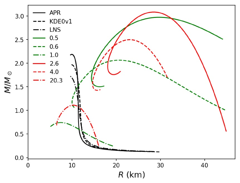
Figure 1: Mass-radius relations for different compact stars. Pure NM neutron stars (black lines) are modeled by the APR, KDE0v1, and LNS EOSs. Fermionic DM stars (green lines) modeled by ideal Fermi gas EOS are labeled by the particle mass $\mu$ (in GeV). Bosonic DM stars (red lines) are labeled by $\rho_{0}\hbar^{3}$ (in $10^{-4}$ GeV⁴).

The tidal Love number and dimensionless tidal deformability of the stars shown in Fig. 1 are plotted against the total mass $M$ in Fig. 2 and Fig. 3, respectively. These plots give us some understanding about each EOS. Indeed, the $\Lambda-M$ relation normalized by the $M_{max}$ of each curve is independent of the particle mass, for both fermionic and bosonic DM. The dimensionless tidal deformability is sensitive to $\mu$ ($\rho_{0}$) for the fermionic (bosonic) DM EOS, as the horizontal axis of $\Lambda-M$ relation scales with $M_{max}$, which depends on $\mu$ ($\rho_{0}$). For example, a 2.6 $M_{\odot}$ DM star may have a $\Lambda$ around a few hundreds if the $M_{max}$ is around 2.6 $M_{\odot}$, but it will become a few thousands if the $M_{max}$ is 2.9 $M_{\odot}$ instead.

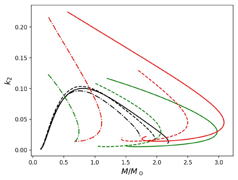
Figure 2: Tidal Love number against total mass for the same EOSs and parameters as those in Fig. 1 .

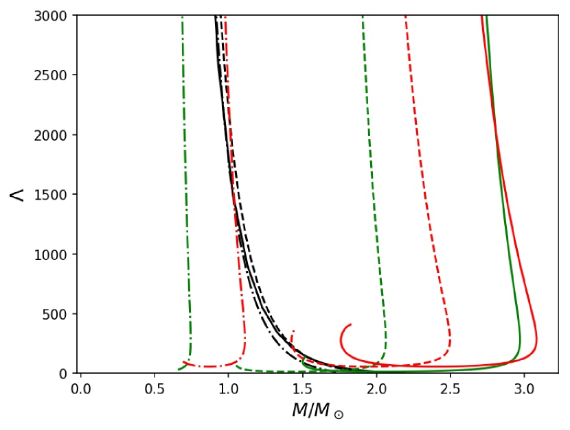
Figure 3: Same as Fig. 2, but for the dimensionless tidal deformability.

III Result

III.1 DM Admixed Neutron Stars with Various DM Mass Fractions

After considering our models of pure NM neutron stars, fermionic, and bosonic DM stars, we now study more generally the properties of DM-admixed compact stars using a two-fluid description. In Fig. 4, we show the mass-radius relation of two-fluid stars with different DM mass fractions, constructed with the APR EOS and 0.5 GeV fermionic DM particle mass. The DM mass fraction $f$ is defined as the ratio of the DM mass to the total mass of the star. The shape of the line for $f=0.1$ in Fig. 4 is similar to that of a pure NM star, except for a segment showing a different trend for mass smaller than 1.3 $M_{\odot}$. The $f=0.1$ curve starts to deviate to a larger radius. This tail behaves more similar to the pure DM ($f=1$) curve, with a more gentle slope. It is found that kinks on a curve appear when the two components have the same radius. This property may play a role in the tidal properties of a star as they are related to the compactness of the star [58, 68], which is the ratio of the total mass to the outer radius. Similar results are observed when the bosonic EOS is used (Fig. 5). In Fig. 5, there are two kinks for $f=0.1$ and $0.2$. For $f=0.1$, the two kinks are near $R=10$ km. For $f=0.2$, one of the kinks is near $R=10$ km and the other is near $R=16$ km. The segment in between the two kinks concaves downward, similar to the pure DM ($f=1$) curve, but not the pure NM ($f=0$) curve that concaves upward. The segments separated by a kink have similar shapes as those of either the pure NM or pure DM limit. A segment of the mass-radius curve is similar to that of the component with the larger radius. For larger $f$, only one kink is observed near $M=0.3M_{\odot}$ of each curve. The configurations on the flat tails have NM components that are more extended than the DM. The shapes of the tails are all similar to that of the pure NM limit, whereas the pure DM case has no flat tail. This indicates that these flat tails exist because of the extended NM component. The configurations on the flat tails have very low mass and large radius, or very low compactness. Therefore, these configurations are not in the range of our interest even if they are stable. Similar results can also be observed for other EOSs. We will see later that the relative sizes of the two components play an important role in admixed stars.

In Figs. 6 and 7, we plot the NM and DM density profiles of two particular star models in Fig. 5 as an illustration. They have the same compactness $\beta=0.255$ but different $f$. For the model in Fig. 6, the DM radius is smaller than the NM radius and the DM mass only contributes $10\%$ of the total mass. However, the DM of the model in Fig. 7 is the larger component and has a higher density near the core. We expect these configurations to show different tidal properties. The tidal properties of a star may indicate the existence of a second admixed fluid.

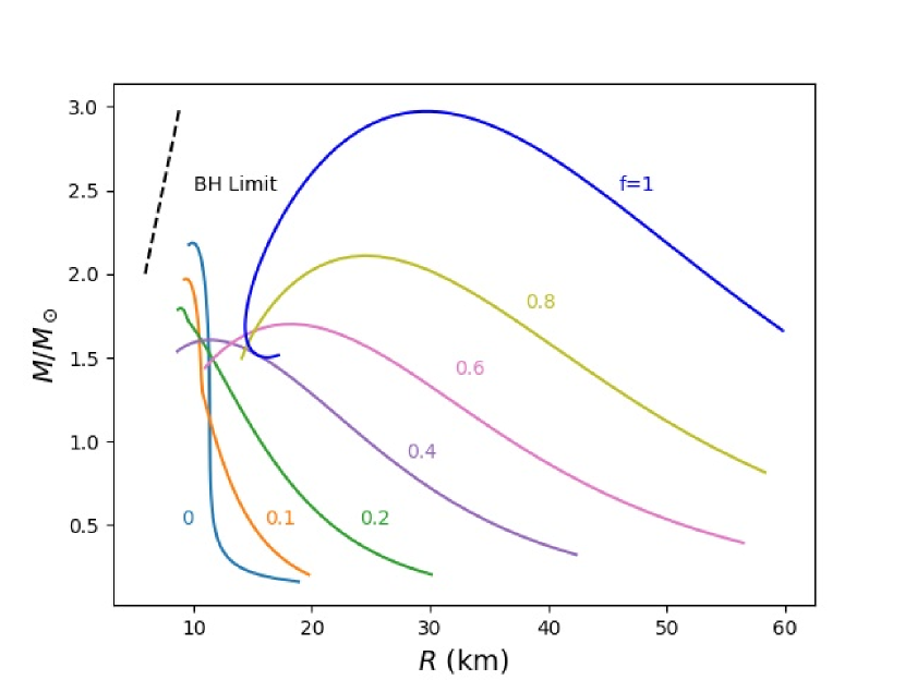
Figure 4: Mass-radius relations of DM-admixed compact stars constructed with the APR EOS and $\mu=$ 0.5 GeV fermionic DM EOS for different DM fractions $f$. The dashed line is the black hole limit.

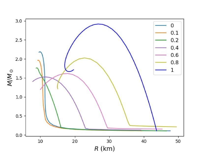
Figure 5: Same as Fig. 4, but with the APR EOS and $\rho_{0}\hbar^{3}=2.93\times 10^{-4}$ GeV⁴ bosonic DM EOS.

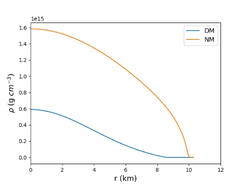
Figure 6: Density profile of a configuration in Fig. 5, where $\beta=0.255$ and $f=0.1$.

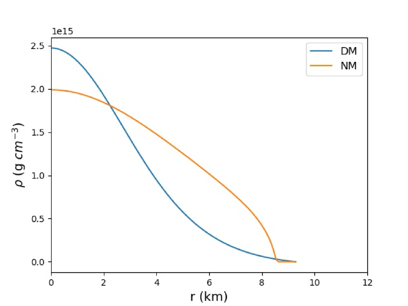
Figure 7: Same as Fig. 6, but with $f=0.3$.

In Figs. 8 and 9, the mass-radius relations are generated by the same NM EOS but with different DM EOSs. The NM EOS is LNS, while the DM EOS is ideal Fermi gas, with DM particle mass of 1.0 GeV (Fig. 8) or 0.6 GeV (Fig. 9). The $M_{max}$ of pure DM stars for $\mu=$ 0.6 GeV (1.0 GeV) is greater (smaller) than that of the NM EOS (see Fig. 1). In both cases, the additional component does not increase $M_{max}$, which occurs either in the pure DM or pure NM stars. This is also true for other EOSs we have used. Gravity is contributed by both fluids, but the pressure of each fluid can only support the corresponding fluid itself. It is not surprising that a two-fluid star cannot support as much total mass as the one-fluid limit.

It was suggested in [69] that the stability of DM-admixed neutron stars can be deduced from the $M-\rho_{c}$ relation for a fixed $f$ in the same way as for one-fluid stars. The turning point on a given mass-radius relation represents the maximum stable mass configuration. The stars beyond the turning point (on the branch of smaller $R$) are unstable against radial perturbations.

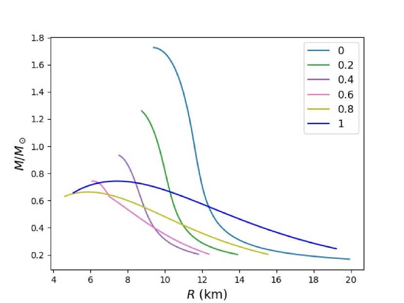
Figure 8: Same as Fig. 4, but with the LNS EOS and $\mu=$ 1.0 GeV.

Figure 9: Same as Fig. 4, but with the LNS EOS and $\mu=$ 0.6 GeV.

A kink similar to those in Figs. 4 and 5 is observed in the tidal Love number against total mass curve, and is more significant. Fig. 10 shows the results for the LNS EOS with $\mu=0.6$ GeV as an example. We can see that the tidal Love number may drop to a half or even less as $f$ is increased for a fixed total mass. Relations between $k_{2}$ and $M$ for neutron stars modeled by different nuclear matter EOSs were studied in [68]. For $f=0.1$, the change in $k_{2}$ relative to a pure NM neutron star is not significant compared with the differences arising from different neutron star EOSs. So, for such a small amount of DM admixed, it would be difficult to distinguish a DM admixed neutron star from a traditional neutron star without DM through the tidal Love number. However, the situation is different for $f=0.2$. For $M<$ 1.25 $M_{\odot}$, $k_{2}$ decreases significantly compared to the pure NM result, by more than 50%. The kink on the $k_{2}-M$ relation induces a large change in $k_{2}$, which may be a possible signature of DM-admixed neutron stars. These kinks will be significant only for some range of $f$, possibly due to the fact that the two components may have the same radius only for some $f$. Similar results can be observed with other choices of EOS, but the positions of the kinks, the range of $f$ that the kinks are present and the change in the value of $k_{2}$ are sensitive to the EOS.

Figure 10: Same as Fig. 9, but for the tidal Love number against total mass.

It is interesting to understand why and how the tidal Love number changes when DM is admixed. For better comparison, we plot the tidal Love number against compactness in Fig. 11. There are kinks on the lines with $f=0.2$ (around $\beta=0.19$) and $f=0.3$ (around $\beta=0.24$). These kinks are located near the configuration with the same NM and DM radii. The $k_{2}-\beta$ curves are similar for $f=0,0.1$, and the right half of $f=0.2$. Before the DM component takes up a larger radius than the NM’s, the effect of the DM admixture simply shifts the $k_{2}-\beta$ curve but preserves its general shape. For $f>0.5$, the tidal Love number decreases when the compactness increases monotonically. This trend has also been observed for polytropic star models [56]. As our DM EOSs are similar to the polytropic EOS, it is not surprising that our results for high DM fraction show a similar trend.

Figure 11: Same as Fig. 10, but for the tidal Love number against compactness.

Interestingly, when $\beta$ is around 0.05 to 0.20 and $f$ is around 0.2 to 0.4, the tidal Love number is significantly lower than that of the pure NM case. Several NM EOSs were studied in [56], and it was shown that the tidal Love number for a pure NM neutron star typically peaks at around 0.1 to 0.15. By considering the profile of $y(r)$ defined in Eq. 9 and its value at the surface $y_{R}$, we find that the low density region of a star plays a role in the suppression of the tidal Love number when DM is admixed. We have studied the configurations around the kink ($\beta=0.18$) on the $f=0.2$ line in Fig. 11. In Fig. 12, we plot the profiles of $y(r)$ for $\beta=0.18$ and different $f$. For $f<0.2$, the v-shape curves are shifted to smaller radius when $f$ increases, while $y_{R}$ remain more or less the same. However, for $f>0.2$, the v-shape curves have a much longer extension of positive slope side, and they also shift upwards as $f$ increases. Thus, the values of $y_{R}$ for $f>0.2$ are much larger than those of $f<0.2$. Although the tidal Love number $k_{2}(\beta,y_{R})$ is a complicated function of $\beta$ and $y_{R}$, in the region we are interested in, $k_{2}$ decreases when $y_{R}$ increases. Thus, we get a much lower tidal Love number for $f>0.2$. Moreover, the v-shape in the $y(r)$ curve is confined to the low density region of the star. In Fig. 13, we plot the total energy density profiles for the star models corresponding to the results presented in Fig. 12. It is noted that the minima of the v-shape curves in Fig. 12 are located near the positions where the density is very low and its slope has a drastic change. For $f<0.2$, the NM is still the larger component, and the DM component only affects the surface distribution of NM slightly, resulting in only small changes in $y(r)$, $y_{R}$, and therefore $k_{2}$. For $f>0.2$, the DM becomes the larger component and contributes to much larger $y(r)$, $y_{R}$, and therefore lower $k_{2}$. Similar results are observed by fixing $f$ but varying $\beta$.

Figure 12: Profiles of $y(r)$ for $\beta=0.18$ and different $f$ from 0.05 to 0.40. Same setting as Fig.11

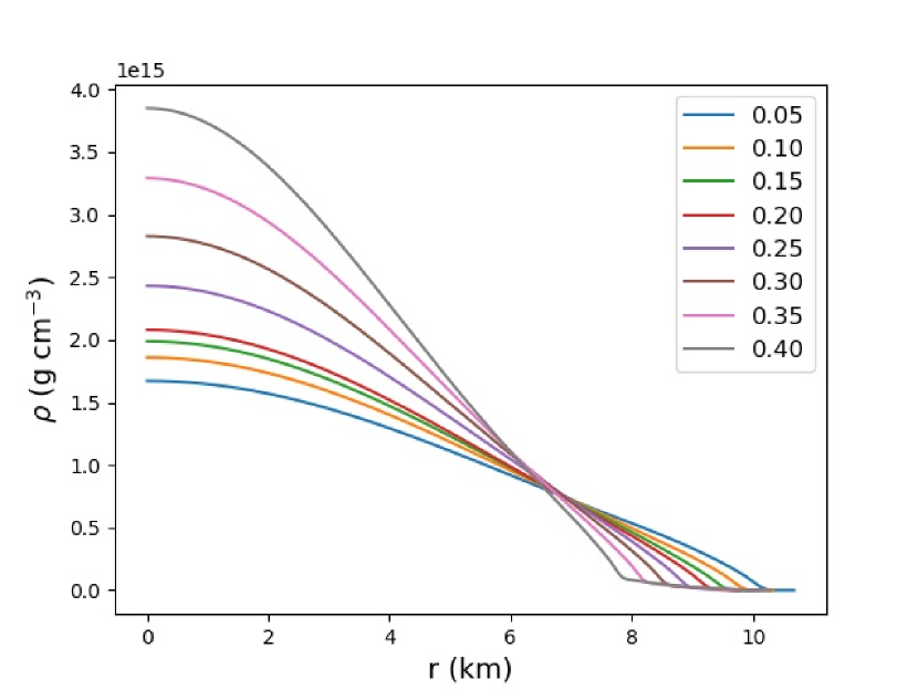
Figure 13: Total energy density profiles for $\beta=0.18$. Same setting as Fig.11

Let us now focus on the case that the $M_{max}$ of the DM EOS is larger than that of the NM EOS. Fig. 14 is similar to Fig. 10, but for the dimensionless tidal deformability againist total mass. Unlike the previous results in Figs. 4 and 10, the curves are generally smooth. For $f<0.2$, the $\Lambda-M$ curves are similar to each other.. For example, for $M=$ 1.25 $M_{\odot}$, the dimensionless tidal deformability of the $f=0.2$ case is around 70% smaller than that of a pure neutron star, and is around 85% smaller for 1.4 $M_{\odot}$. This result agrees with that in [42], which shows that a $M=1.4M_{\odot}$ neutron star will have a smaller $\Lambda$ when a small amount of DM is admixed. The DM-admixed $\Lambda-M$ curves are shifted to smaller stellar mass compared with that of the pure NM case, and thus, $\Lambda$ is decreased for a fixed stellar mass but larger $f$. This seems to be a general property regardless of the mass of the star.

The dimensionless tidal deformability starts to increase for $f>0.4$ in Fig. 14. The curves for $f=0.5$ to $0.7$ are steep. The separations between the curves are larger than those with $f<0.5$. This indicates that $\Lambda$ is very sensitive to $M$ and $f$. $\Lambda$ increases rapidly when $f$ increases in this range. A change in $f$ will shift the curve horizontally on the graph, which gives a rapid change in $\Lambda$. The large range of possible $\Lambda$ values may save some NM EOSs from being ruled out by observations with $f$ as an extra degree of freedom. However, it will also be difficult to distinguish and select the NM EOSs and constrain the DM parameters in this range of DM fractions, for which a DM halo is formed. A similar rapid increase in $\Lambda$ is also observed for the DM halo models studied in [45]. Qualitatively similar results can be observed for other choices of the EOS. For example, the APR EOS with 0.4 GeV fermionic DM particle mass shows similar results, but $\Lambda$ starts to increase at around $f=0.1$ instead. Note that we have only considered the cases where the DM EOS has a larger $M_{max}$ than that of the NM. For the opposite situation where the DM EOS has a smaller $M_{max}$ than that of the NM EOS, we consider the KDE0v1 EOS with $\mu=$ 1.0 GeV as an example, and the corresponding $\Lambda-M$ relation is shown in Fig. 15. The curves are almost vertical for $f>0.5$. The $\Lambda$ is thus sensitive to $M$. Qualitatively similar results can be observed for other choices of the EOS.

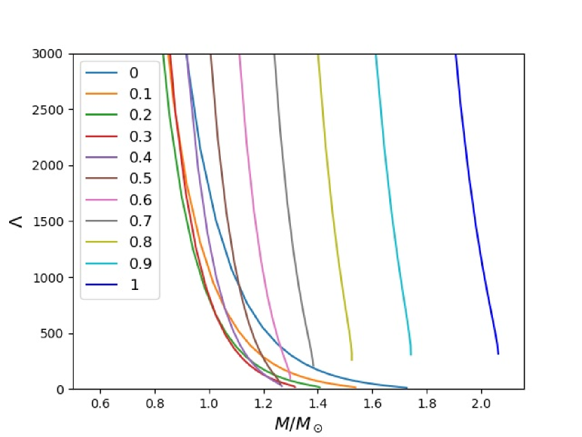
Figure 14: Same as Fig. 10, but for the dimensionless tidal deformability.

In all the results we have shown, the properties of two-fluid stars show continuous change between the limits of pure NM and pure DM stars, with an abrupt transition at an intermediate DM mass fraction. The $\Lambda-M$ curves become steep at some intermediate DM fractions, implying that $\Lambda$ will be very sensitive to the $M$ and $f$. Also, for DM EOS with smaller $M_{max}$, the slope of the $\Lambda-M$ curve is steeper, so that $\Lambda$ is sensitive to $M$. For DM EOS with larger $M_{max}$, the separation between the curves at intermediate DM fractions is large, so that $\Lambda$ is sensitive to $f$.

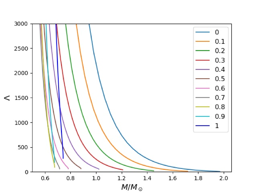
Figure 15: Same as Fig. 14, but for the KDE0v1 EOS with $\mu=1.0$ GeV.

In Fig. 16, we plot $\Lambda$ against $M/M_{max}$ for different $f$. The normalized relation is less sensitive to $f$, when $f$ is high ( $>0.8$ in this example). This result is similar to the fact that properties of DM stars for the DM EOSs we considered are self-similar and scale with $M_{max}$, for different DM parameters. The large separation between the curves in Fig. 14 indicates that $\Lambda$ is very sensitive to both $f$ and $M$ in this range. However, we may utilize the result that the $\Lambda-M$ relations are self-similar for large $f$, so that we can reduce the relations to a single one for $M/M_{max}$. So, we may study the relation between $M_{max}$ and $f$, instead of that of $\Lambda$ and $f$. Also, although $f=0.7$ is not perfectly fitted, it is still approximately the same as the others, except a few percentage shift along $M/M_{max}$. Similar behaviour can be observed with other choice of EOS when the DM EOS has a greater maximum mass than that of NM.

Also, except for $f>0.8$, where the $\Lambda-M/M_{max}$ curves are similar, the $\Lambda-M/M_{max}$ curves of smaller $f$ are always on the left of those for higher $f$, and there is no crossing between the curves. This is different from Fig. 14, where the $\Lambda-M$ curves move back and forth along the horizontal direction and cross with others. The transition from pure NM to pure DM is clearer after we normalize $M$ by $M_{max}$. This suggests that $\Lambda$ should be studied as a function of both $M$ and $M/M_{max}$.

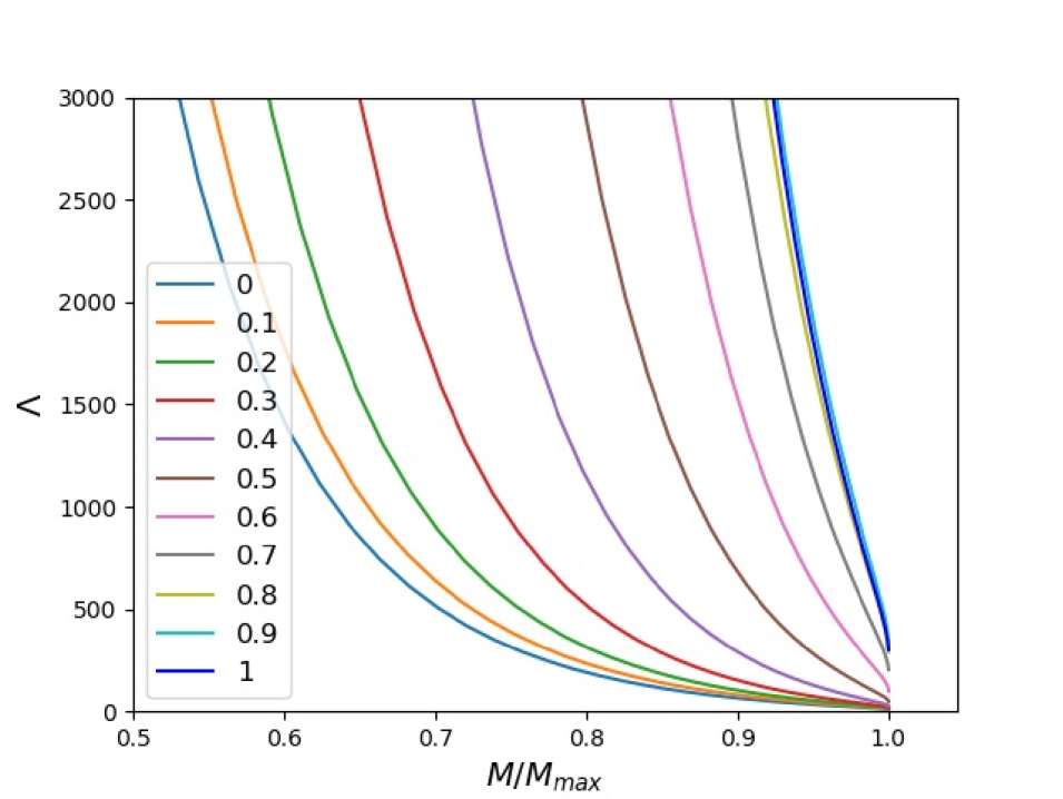
Figure 16: Same as Fig. 14, but with the total mass normalized by $M_{max}$ of each curve.

III.2 Massive DM-Admixed Neutron Stars

In the future, more gravitational-wave events similar to GW190814 may be observed. Although the tidal properties were not measured for the GW190814 $2.6M_{\odot}$ compact object, we will use it as an example to study compact objects in the mass gap.

The nature of the 2.6 $M_{\odot}$ object is still unknown. It may be the lowest-mass black hole ever observed, or the largest-mass neutron star. The pure NM neutron stars constructed from the EOSs we use, as well as those from many other EOSs, cannot reach 2.6 $M_{\odot}$. The 2.6 $M_{\odot}$ object could be a DM-admixed neutron star or even a pure DM star, and if so, we may constrain the range of DM parameters. It is found that even admixed with DM, a two-fluid star will only reach its maximum mass at either the pure NM or pure DM limits. So, the DM-admixed neutron star allows a maximum mass of 2.6 $M_{\odot}$ only if the DM EOS can reach 2.6 $M_{\odot}$. Indeed, $M_{max}=2.6M_{\odot}$ can be reached if $\mu<0.535$ GeV for fermionic DM and $\rho_{0}\hbar^{3}<3.69\times 10^{-4}$ GeV⁴ for bosonic DM. A much higher mass limit for the DM EOS can be achieved if we consider a smaller DM particle mass. However, the radius and $\Lambda$ of such a DM star will also increase significantly. Other constraints may be applied, such as the radius of the DM component should be within the binary system, and the star should be stable against tidal disruption during the inspiral phase.

Furthermore, if the tidal properties of the binary system are measured, we may narrow down the DM parameter space. When the DM fraction is high, we have shown that the $\Lambda-M$ relations are similar to that of the pure DM stars if they are normalized by $M_{max}$. This indicates that they share approximately the same dimensionless function, i.e. the relations can be written as

$$\Lambda(M/M_{max}(f);\sigma)\approx\Lambda(M/M_{max}(f=1);\sigma),$$ (24)

where $\sigma$ denotes the parameter for the DM EOS. Also, as mentioned, the DM EOSs we use are self-similar, which means that they share the same dimensionless function that is independent of the parameter:

$$\Lambda(M/M_{max}(f=1);\sigma)=\Lambda(M/M_{max}(f=1)).$$ (25)

Therefore, all these $\Lambda-M$ relations share approximately the same dimensionless function. All the information are described by the normalizing factor, which is the maximum mass of a $\Lambda-M$ relation, with a given NM EOS, fixed DM parameters and a fixed DM fraction $f$. By considering the maximum mass with different combinations of parameters, we may give constraints to the parameter space.

We demonstrate the approach with an example. Assume we have observed a star with mass in between [2.55,2.65] $M_{\odot}$ with $\Lambda$ in between [1000, 2000]. We assume NM EOS to be APR EOS and DM EOS bosonic. In Fig. 17, we can limit the range of the $M/M_{max}$ by $\Lambda$. Although the $\Lambda-M$ relations with high DM fraction is not perfectly fitted on the dimensionless form, they behave like shifting along the axis with a few percentage deviation. So, we may include this approximation in the range of mass. Thus, the range of $M/M_{max}$ lies in approximately [0.90, 0.97], and the maximum mass will be in [2.63, 2.94] $M_{\odot}$. Fig. 18 shows a contour plot for the maximum mass as a function of the DM fraction and $\rho_{0}\hbar^{3}$. The parameter space is then constrained. Although the NM EOS is still unknown, this approach can be carried out with different NM EOSs and then the results combined. This graph only shows a range of parameters. It is possible to extend the axis of $\rho_{0}\hbar^{3}$ to even lower values, but there may be some constraints as mentioned before. We have not ruled out the low DM fraction part, but that is the case that this approach cannot be directly applied to. Also, the way to define “high” DM fraction needs further work.

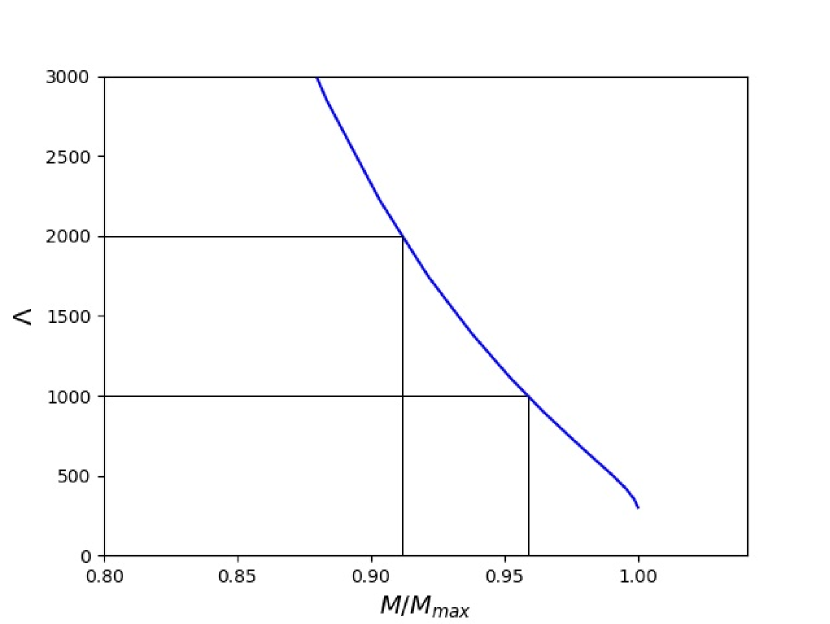
Figure 17: $\Lambda-M$ relation for bosonic DM EOSs, with $M$ normalized by the maximum mass. Black lines indicate the range of variables as the example.

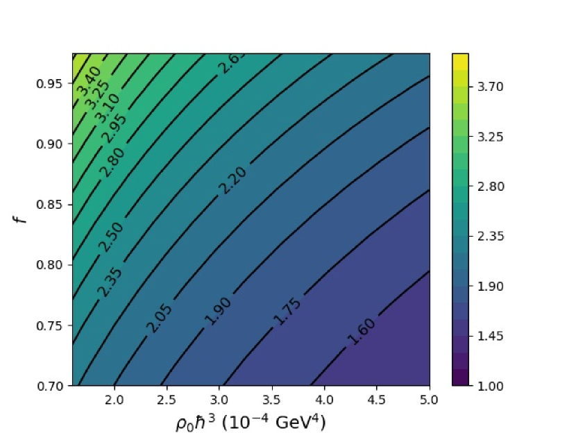
Figure 18: A contour plot of maximum mass as a function of DM fraction and $\rho_{0}\hbar^{3}$. APR EOS are assumed for NM, and bosonic DM are assumed.

IV Discussion

We have studied the static configurations and tidal properties of DM admixed neutron stars. We observe drastic changes (kinks) in the tidal Love number as a function of compactness or stellar mass when the NM and DM components have the same radius. For small (large) $f$, the tidal Love number behaves similar to that of a pure NM (DM) star as expected. However, for intermediate values of $f$, such as around 0.3, the tidal Love number is much reduced relative to that of a pure NM star. We find that in such cases, the DM component has a low density tail engulfing the NM component, which leads to a significant decrease of the tidal Love number. Also, we have studied the dimensionless tidal deformability $\Lambda$. For small $f$, where the star configuration is similar to a pure NM star, $\Lambda$ will tend to decrease when more DM are admixed. For large $f$, where the star configuration is similar to a pure DM star, the $\Lambda-M$ curves can be scaled to that of the pure DM stars. Further study about the similarity of $\Lambda(M/M_{Max})$ for different $f$ may help to relate the properties of pure DM stars to those for stars with large $f$. The tidal properties of stars with intermediate DM fractions are much more sensitive to the DM parameters.

The existence of the DM component hardly helps to increase the total mass of the star unless the DM fraction is high. However, this means that the two-fluid star is more like a DM star instead of a neutron star. A pure DM star can have a $M_{max}$ larger than that of the two-fluid stars. Therefore, we may make use of massive compact object in GW190814 [23] as DM-admixed stars to limit the DM parameter space, if such a star is believed to have a high DM fraction. If the recently discovered 2.6 $M_{\odot}$ compact object is a DM-admixed neutron star with a high DM fraction, the fermionic DM would have $\mu<0.535$ GeV, and the self-interacting bosonic DM would have $\rho_{0}\hbar^{3}<3.69\times 10^{-4}$ GeV⁴. Any more massive compact objects that are not black holes, if detected, will give even tighter constraints on these DM parameters, provided that these star have a high DM fraction. For compact objects in the mass gap, we have also illustrated a method to limit the DM parameters and DM fraction if the DM fraction is high.

Appendix A Derivation from General Relativistic Two-fluid Formalism

We follow the general relativistic two-fluid formalism used in [53] and [69]. We will use a similar notation as [69], except that the number density current for DM will be denoted as $d^{\alpha}$ and the master function will be denoted as $\Phi$. The master function plays the role of EOS in the two-fluid formalism and is defined by the number density currents of the two fluids as discussed below. The Einstein field equation and the hydrodynamics equations reduce to the following equations by considering a static and spherically symmetric spacetime [69] ,

$$\lambda^{\prime}=\frac{1-e^{\lambda}}{r}-8\pi re^{\lambda}\Phi,$$ (26)

$$\nu^{\prime}=-\frac{1-e^{\lambda}}{r}+8\pi re^{\lambda}\Psi,$$ (27)

$$A^{0}_{0}d^{\prime}+B^{0}_{0}n^{\prime}+\frac{1}{2}(Bn+Ad)\nu^{\prime}=0,$$ (28)

$$C^{0}_{0}d^{\prime}+A^{0}_{0}n^{\prime}+\frac{1}{2}(An+Cd)\nu^{\prime}=0,$$ (29)

where the prime denotes the derivative with respect to $r$, and

$$A=-\frac{\partial\Phi}{\partial(x^{2})},B=-2\frac{\partial\Phi}{\partial(n^{2})},C=-2\frac{\partial\Phi}{\partial(d^{2})},$$ (30)

$$A^{0}_{0}=A+2\frac{\partial B}{\partial(d^{2})}nd+2\frac{\partial A}{\partial(n^{2})}n^{2}+2\frac{\partial A}{\partial(d^{2})}d^{2}+\frac{\partial A}{\partial(x^{2})}dn,$$ (31)

$$B^{0}_{0}=B+2\frac{\partial B}{\partial(n^{2})}n^{2}+4\frac{\partial A}{\partial(n^{2})}nd+\frac{\partial A}{\partial(x^{2})}d^{2},$$ (32)

$$C^{0}_{0}=C+2\frac{\partial C}{\partial(d^{2})}d^{2}+4\frac{\partial A}{\partial(d^{2})}nd+\frac{\partial A}{\partial(x^{2})}n^{2},$$ (33)

where $n^{2}$, $d^{2}$, and $x^{2}$ are scalars defined by the NM $n^{\mu}$ and DM $d^{\mu}$ number density currents:

$$n^{2}=-n_{\alpha}n^{\alpha},d^{2}=-d_{\alpha}d^{\alpha},x^{2}=-n_{\alpha}d^{\alpha}.$$ (34)

The master function $\Phi$ is in general a function of $n^{2}$, $d^{2}$, and $x^{2}$. The generalized pressure $\Psi$ is given by

$$\Psi=\Phi+\mu n+\chi d,$$ (35)

where $\mu=Bn+Ad$ and $\chi=Cd+An$ are the chemical potentials of NM and DM, respectively. With a given master function and suitable boundary conditions, the above equations can be used to construct a non-rotating two-fluid star in general relativity [53, 69].

Now, we make the assumption that NM and DM only interact with each other through gravity. This means that the two fluids affect each other only through the effect of the metric. This assumption means that the master function $\Phi$ does not depend on the cross term $x^{2}$ so that $\Phi$ can be separated into two parts,

$$\Phi(n^{2},d^{2},x^{2})=\Phi_{n}(n^{2})+\Phi_{d}(d^{2}).$$ (36)

With this assumption, many of the above coefficients can be simplified:

$$A=A^{0}_{0}=0,$$ (37)

$$B=-\frac{1}{n}\frac{\partial\Phi_{n}}{\partial n},C=-\frac{1}{d}\frac{\partial\Phi_{d}}{\partial d},$$ (38)

$$B^{0}_{0}=B+\frac{\partial B}{\partial n}n,C^{0}_{0}=C+\frac{\partial C}{\partial d}d.$$ (39)

The generalized pressure $\Psi$ can also be separated into two parts as $\Psi=\Psi_{n}(n^{2})+\Psi_{d}(d^{2})$, where

$$\Psi_{n}=\Phi_{n}(n^{2})+Bn^{2},$$ (40)

$$\Psi_{d}=\Phi_{d}(d^{2})+Cn^{2}.$$ (41)

It is noticed that

$$\frac{\partial\Psi_{n}}{\partial n} =\frac{\partial(\Phi_{n}+Bn^{2})}{\partial n}=Bn+\frac{\partial B}{\partial n}n^{2}=B^{0}_{0}n.$$ (42)

We can substitute Eq.s 37 to 42 into Eq. 28 to get

$$\frac{d\Psi_{n}}{dr}=-\frac{1}{2}(-\Phi_{n}+\Psi_{n})\nu^{\prime}.$$ (43)

Same result is also obtained for the DM part. By setting one of the components to have zero contribution, the standard TOV equation shall be obtained. We shall replace the generalized pressure $\Psi_{i}$ by the usual pressure $p_{i}$, and master function $\Phi_{i}$ by the minus of energy density $-\rho_{i}$. The set of two-fluid equations is then obtained in the form of the standard TOV equation. We can also check the relation between $\Phi_{i}$ and $\Psi_{i}$ to see if they fulfill the same relation between the energy density and pressure. From thermodynamics, we have the following relation,

$$p_{n}=-\frac{\partial(\rho_{n}/n)}{\partial(1/n)}=\frac{\partial\rho_{n}}{\partial n}n-\rho_{n}.$$ (44)

From Eq.s 38 and 40, we have

$$\Psi_{n}=-(-\Phi_{n})+\frac{\partial(-\Phi_{n})}{\partial n}n.$$ (45)

Similar results can be obtained for both fluids.

To compute the tidal Love number, we follow the method in [59, 60]. The modification for Eq. 10 is

$$\frac{\rho+p}{dp/d\rho}\to -\frac{\mu^{2}C^{0}_{0}+\chi^{2}B^{0}_{0}-2\mu\chi A^{0}_{0}}{{A^{0}_{0}}^{2}-B^{0}_{0}C^{0}_{0}}$$

$$= \frac{\mu^{2}}{B^{0}_{0}}+\frac{\chi^{2}}{C^{0}_{0}}$$

$$= \sum_{i}\frac{\rho_{i}+p_{i}}{dp_{i}/d\rho_{i}}.$$ (46)

References

- Bertone et al. [2005] G. Bertone, D. Hooper, and J. Silk, Phys. Rep. 405, 279 (2005).
- Begeman et al. [1991] K. G. Begeman, A. H. Broeils, and R. H. Sanders, Mon.Not. R. Astron. Soc. 249, 523 (1991).
- Hu and Dodelson [2002] W. Hu and S. Dodelson, Annu. Rev. Astron. Astrophys. 40, 171 (2002).
- Wittman et al. [2000] D. Wittman, J. Tyson, D. Kirkman, and et al., Nature 405, 143 (2000).
- et al [2010] R. M. et al, Rep. Prog. Phys. 73, 086901 (2010).
- et al [2016] S. A. et al, Rep. Prog. Phys. 79, 124201 (2016).
- Essig et al. [2012] R. Essig, A. Manalaysay, J. Mardon, P. Sorensen, and T. Volansky, Phys. Rev. Lett. 109, 021301 (2012).
- et al [2020] E. A. et al (XENON Collaboration), Phys. Rev. D 102, 072004 (2020).
- Ozel and Freire [2016] F. Ozel and P. Freire, Annu. Rev. Astron. Astrophys. 54, 401 (2016).
- Lattimer and Prakash [2007] J. Lattimer and M. Prakash, Phys. Rep. 442, 109–165 (2007).
- Chatziioannou [2020] K. Chatziioannou, Gen. Relativ. Gravit. 52, 109 (2020).
- Adhikari et al. [2021] D. Adhikari et al. (PREX Collaboration), Phys. Rev. Lett. 126, 172502 (2021).
- Demorest et al. [2010] P. Demorest, T. Pennucci, S. Ransom, M. Roberts, and J. Hessels, Nature 467, 1081 (2010).
- Antoniadis et al. [2013] J. Antoniadis, P. C. C. Freire, N. Wex, and et al, Science 340 (2013).
- Abbott et al. [2017] B. P. Abbott et al. (LIGO Scientific Collaboration and Virgo Collaboration), Phys. Rev. Lett. 119, 161101 (2017).
- Abbott et al. [2018] B. P. Abbott et al. (The LIGO Scientific Collaboration and the Virgo Collaboration), Phys. Rev. Lett. 121, 161101 (2018).
- Annala et al. [2018] E. Annala, T. Gorda, A. Kurkela, and A. Vuorinen, Phys. Rev. Lett. 120, 172703 (2018).
- De et al. [2018] S. De, D. Finstad, J. M. Lattimer, D. A. Brown, E. Berger, and C. M. Biwer, Phys. Rev. Lett. 121, 091102 (2018).
- Fattoyev et al. [2018] F. J. Fattoyev, J. Piekarewicz, and C. J. Horowitz, Phys. Rev. Lett. 120, 172702 (2018).
- Most et al. [2018] E. R. Most, L. R. Weih, L. Rezzolla, and J. Schaffner-Bielich, Phys. Rev. Lett. 120, 261103 (2018).
- Tews et al. [2018] I. Tews, J. Margueron, and S. Reddy, Phys. Rev. C 98, 045804 (2018).
- Lim and Holt [2018] Y. Lim and J. W. Holt, Phys. Rev. Lett. 121, 062701 (2018).
- Abbott et al. [2020] R. Abbott et al. (LIGO Scientific Collaboration and Virgo Collaboration), Astrophys. J. 896, L44 (2020).
- Most et al. [2020] E. R. Most, L. J. Papenfort, L. R. Weih, and L. Rezzolla, Mon. Not. R. Astron. Soc. 499, L82 (2020).
- Essick and Landry [2020] R. Essick and P. Landry, Astrophys. J. 904, 80 (2020).
- Zhang and Li [2020] N.-B. Zhang and B.-A. Li, Astrophys. J. 902, 38 (2020).
- Tsokaros et al. [2020] A. Tsokaros, M. Ruiz, and S. L. Shapiro, Astrophys. J. 905, 48 (2020).
- Dexheimer et al. [2021] V. Dexheimer, R. O. Gomes, T. Klähn, S. Han, and M. Salinas, Phys. Rev. C 103, 025808 (2021).
- Fattoyev et al. [2020] F. J. Fattoyev, C. J. Horowitz, J. Piekarewicz, and B. Reed, Phys. Rev. C 102, 065805 (2020).
- Tews et al. [2021] I. Tews, P. T. H. Pang, T. Dietrich, M. W. Coughlin, S. Antier, M. Bulla, J. Heinzel, and L. Issa, Astrophys. J. 908, L1 (2021).
- Riley et al. [2019] T. E. Riley et al., Astrophys. J. 887, L21 (2019).
- Miller et al. [2019] M. C. Miller et al., Astrophys. J. 887, L24 (2019).
- Riley et al. [2021] T. E. Riley et al., Astrophys. J. Lett. 918, L27 (2021).
- Miller et al. [2021] M. C. Miller et al., Astrophys. J. Lett. 918, L28 (2021).
- Chan et al. [2021] H.-S. Chan, M.-C. Chu, S.-C. Leung, and L.-M. Lin, Astrophys. J. 914, 138 (2021).
- Leung et al. [2015] S.-C. Leung, M.-C. Chu, and L.-M. Lin, Astrophys. J. 812, 110 (2015).
- Ciarcelluti and Sandin [2011] P. Ciarcelluti and F. Sandin, Phys. Lett. B 695, 19 (2011).
- Leung et al. [2011] S.-C. Leung, M.-C. Chu, and L.-M. Lin, Phys. Rev. D 84, 107301 (2011).
- Xiang et al. [2014] Q.-F. Xiang, W.-Z. Jiang, D.-R. Zhang, and R.-Y. Yang, Phys. Rev. C 89, 025803 (2014).
- Rezaei [2017] Z. Rezaei, Astrophys. J. 835, 33 (2017), arXiv:1612.02804 [astro-ph.HE] .
- Ellis et al. [2018a] J. Ellis, A. Hektor, G. Hütsi, K. Kannike, L. Marzola, M. Raidal, and V. Vaskonen, Phys. Lett. B 781, 607 (2018a).
- Ellis et al. [2018b] J. Ellis, G. Hütsi, K. Kannike, L. Marzola, M. Raidal, and V. Vaskonen, Phys. Rev. D 97, 123007 (2018b).
- Gresham and Zurek [2019] M. I. Gresham and K. M. Zurek, Phys. Rev. D 99, 083008 (2019).
- Deliyergiyev et al. [2019] M. Deliyergiyev, A. Del Popolo, L. Tolos, M. Le Delliou, X. Lee, and F. Burgio, Phys. Rev. D 99, 063015 (2019).
- Nelson et al. [2019] A. E. Nelson, S. Reddy, and D. Zhou, J. Cosmol. Astropart. Phys. 2019 (07), 012–012.
- Das et al. [2020] H. C. Das, A. Kumar, B. Kumar, S. K. Biswal, T. Nakatsukasa, A. Li, and S. K. Patra, Mon. Not. R. Astron. Soc. 495, 4893–4903 (2020).
- Zhang et al. [2022] K. Zhang, G.-Z. Huang, J.-S. Tsao, and F.-L. Lin, Eur. Phys. J. C 82, 366 (2022).
- Kain [2021] B. Kain, Phys. Rev. D 103, 043009 (2021).
- Lee et al. [2021] B. K. K. Lee, M.-C. Chu, and L.-M. Lin, Astrophys. J. 922, 242 (2021).
- Sennett et al. [2017] N. Sennett, T. Hinderer, J. Steinhoff, A. Buonanno, and S. Ossokine, Phys. Rev. D 96, 024002 (2017).
- Maselli et al. [2017] A. Maselli, P. Pnigouras, N. G. Nielsen, C. Kouvaris, and K. D. Kokkotas, Phys. Rev. D 96, 023005 (2017).
- Oppenheimer and Volkoff [1939] J. R. Oppenheimer and G. M. Volkoff, Phys. Rev. 55, 374 (1939).
- Comer et al. [1999] G. L. Comer, D. Langlois, and L. M. Lin, Quasinormal modes of general relativistic superfluid neutron stars, Phys. Rev. D 60, 104025 (1999).
- Hinderer [2008] T. Hinderer, Astrophys. J. 677, 1216–1220 (2008).
- Damour and Nagar [2009] T. Damour and A. Nagar, Phys. Rev. D 80, 084035 (2009).
- Postnikov et al. [2010] S. Postnikov, M. Prakash, and J. M. Lattimer, Phys. Rev. D 82, 024016 (2010).
- Flanagan and Hinderer [2008] E. E. Flanagan and T. Hinderer, Phys. Rev. D 77, 021502 (2008).
- Yagi and Yunes [2013] K. Yagi and N. Yunes, Phys. Rev. D 88, 023009 (2013).
- Char and Datta [2018] P. Char and S. Datta, Phys. Rev. D 98, 084010 (2018).
- Yeung et al. [2021] C.-H. Yeung, L.-M. Lin, N. Andersson, and G. Comer, Universe 7, 111 (2021).
- Colpi et al. [1986] M. Colpi, S. L. Shapiro, and I. Wasserman, Phys. Rev. Lett. 57, 2485 (1986).
- Chavanis [2011] P.-H. Chavanis, Phys. Rev. D 84, 043531 (2011).
- Akmal et al. [1998] A. Akmal, V. R. Pandharipande, and D. G. Ravenhall, Phys. Rev. C 58, 1804 (1998).
- Dutra et al. [2012] M. Dutra, O. Lourenço, J. S. Sá Martins, A. Delfino, J. R. Stone, and P. D. Stevenson, Phys. Rev. C 85, 035201 (2012).
- Cao et al. [2006] L. G. Cao, U. Lombardo, C. W. Shen, and N. V. Giai, Phys. Rev. C 73, 014313 (2006).
- Agrawal et al. [2005] B. K. Agrawal, S. Shlomo, and V. K. Au, Phys. Rev. C 72, 014310 (2005).
- Lattimer [2012] J. M. Lattimer, Annu. Rev. Nucl. Part. Sci. 62, 485 (2012).
- Hinderer et al. [2010] T. Hinderer, B. D. Lackey, R. N. Lang, and J. S. Read, Phys. Rev. D 81, 123016 (2010).
- Leung et al. [2012] S.-C. Leung, M.-C. Chu, and L.-M. Lin, Phys. Rev. D 85, 103528 (2012).