Ramp Metering to Maximize Freeway Throughput under Vehicle Safety Constraints

Abstract

Ramp Metering (RM) is one of the most effective control techniques to alleviate freeway congestion. We consider RM at the microscopic level subject to vehicle following safety constraints for a freeway with arbitrary number of on- and off-ramps. The arrival times of vehicles to the on-ramps, as well as their destinations are modeled by exogenous stochastic processes. Once a vehicle is released from an on-ramp, it accelerates towards the free flow speed if it is not obstructed by another vehicle; once it gets close to another vehicle, it adopts a safe gap vehicle following behavior. The vehicle exits the freeway once it reaches its destination off-ramp. We design traffic-responsive RM policies that maximize the throughput. For a given routing matrix, the throughput of a RM policy is characterized by the set of on-ramp arrival rates for which the queue sizes at all the on-ramps remain bounded in expectation. The proposed RM policies operate under vehicle following safety constraints, where new vehicles are released only if there is sufficient gap between vehicles on the mainline at the moment of release. Furthermore, the proposed policies work in synchronous cycles during which an on-ramp does not release more vehicles than the number of vehicles waiting in its queue at the start of the cycle. All the proposed policies are reactive, meaning that they only require real-time traffic measurements without the need for demand prediction. However, they differ in how they use the traffic measurements. In particular, we provide three different mechanisms under which each on-ramp either: (i) pauses release for a time interval before the next cycle begins, or (ii) adjusts the release rate during a cycle, or (iii) adopts a conservative safe gap criterion for release during a cycle. The throughput of the proposed policies is characterized by studying stochastic stability of the induced Markov chains, and is proven to be maximized when the merging speed at all the on-ramps equals the free flow speed. Simulations are provided to illustrate the performance of our policies and compare with a well-known RM policy from the literature which relies on local traffic measurements.

1 Introduction

Freeway congestion is caused by high demand competing to use the limited supply of the freeway system. One of the most effective tools to combat this congestion is Ramp Metering (RM), which involves controlling the inflow of traffic to the freeway in order to balance the supply and demand and ultimately improve some measure of performance (Papageorgiou and Kotsialos, (2002); Rios-Torres and Malikopoulos, (2016); Lee et al., (2006)). Typically, macroscopic traffic flow models are used to design RM policies. However, these models lack the necessary resolution to ensure the existence of safe merging gaps for vehicles entering from on-ramps. An alternative is the microscopic-level approach which is limited to heuristics or simulations beyond an isolated on-ramp (Rios-Torres and Malikopoulos, (2016); Sun and Horowitz, (2006)). The objective of this paper is to systematically design RM policies at the microscopic level and analyze their system-level performance.

There is an overwhelming body of work on designing RM policies using macroscopic traffic flow models. We review them here only briefly; interested readers are referred to Papageorgiou and Kotsialos, (2002) for a comprehensive review. RM policies can be generally classified as fixed-time or traffic-responsive (Papageorgiou and Kotsialos, (2002)). Fixed-time policies such as Wattleworth, (1965) are fine-tuned offline and operate based on historical traffic data. Due to the uncertainty in the traffic demand and the absence of real-time measurements, these policies would either lead to congestion or under-utilization of the capacity of the freeway (Papamichail et al., (2010)). Traffic-responsive policies, on the other hand, use real-time measurements. These policies can be further sub-classified as local or coordinated depending on whether the on-ramps make use of the measurements obtained from their vicinity (local) or other regions of the freeway (coordinated) (Papageorgiou and Kotsialos, (2002); Papageorgiou et al., (2003)). A well-known example of a local policy is ALINEA (Papageorgiou et al., (1991)) which has been shown, both analytically and in practice, to yield a (locally) good performance. A caveat in employing local policies is that there is no guarantee that they can improve the overall performance of the freeway while providing a fair access to the freeway from different on-ramps (Papamichail et al., (2010)). This motivates the study of coordinated policies such as the ones considered in Papageorgiou et al., (1990); Papamichail et al., (2010); Gomes and Horowitz, (2006).

Despite the wide use of macroscopic traffic flow models in RM design, this approach has some limitations. One of its major limitations is that it does not capture the specific safety requirements for vehicles entering the freeway from the on-ramps. As a result, it does not guarantee the existence of sufficient gaps between vehicles on the mainline to safely accommodate the merging vehicles. Therefore, the merging vehicles may sometimes be forced to merge even if the gap is not safe, or they may not be able to merge at all. To address this limitation, an alternative is the microscopic-level approach which allows to include the safety requirements in the design of RM to optimize the freeway performance (Rios-Torres and Malikopoulos, (2016)). In addition, it allows to naturally incorporate vehicle automation, which can compensate for human errors, or Vehicle-to-Vehicle (V2V) and Vehicle-to-Infrastructure (V2I) communication, which can provide accurate traffic measurements, in the RM design (Sugiyama et al., (2008); Stern et al., (2018); Zheng et al., (2020); Pooladsanj et al., (2020, 2022); Rios-Torres and Malikopoulos, (2016); Li et al., (2013); Lioris et al., (2017)).

The microscopic-level RM problem involves determining the order in which vehicles should cross the merging point of the mainline and the on-ramp, i.e., determining their so-called merging sequence. Previous works have mostly focused on isolated on-ramps to determine the merging sequence, employing various techniques such as minimizing the average time taken by the vehicles to cross the merging point (Raravi et al., (2007)) or simple heuristic rules such as the first-in first-out scheme (Rios-Torres and Malikopoulos, (2016)). However, there has been limited analysis of the broader impact of these designs on the overall freeway performance. For example, do they optimize certain system-level performance? Indeed it is possible that a greedy policy, i.e., a policy where each on-ramp acts independently, limits entry from the downstream on-ramps and thereby creating long queues or congestion.

Motivated by the aforementioned gaps and increasing vehicle connectivity and automation, the primary objective of this paper is to systematically design traffic-responsive RM policies at the microscopic level and analyze their system-level performance. The key performance metric to evaluate a RM policy in this paper is its throughput. For a given routing matrix, the throughput of a RM policy is characterized by the set of on-ramp arrival rates for which the queue sizes at all the on-ramps remain bounded in expectation. Roughly, the throughput determines the highest traffic demand that a RM policy can handle without creating long queues at the on-ramps. For example, in case of an isolated on-ramp, the throughput of any policy cannot exceed the on-ramp’s flow capacity. The throughput is tightly related to, but different than, the notion of total travel time, which is a popular metric in the literature (Gomes and Horowitz, (2006); Hegyi et al., (2005)). In particular, if the demand exceeds a policy’s throughput, then the expected total travel time of an arriving vehicle, from the moment it joins an on-ramp queue until it leaves the freeway, will increase over time, i.e., the later the vehicle arrives, the more total travel time it will experience on average. On the other hand, if the demand does not exceed the throughput, then the expected total travel time is stabilized. In other words, the throughput of a policy determines the demand threshold at which the expected total travel time transitions from being stabilized to being increasing over time. Therefore, it is desirable to design a policy that achieves the maximum possible throughput among all policies; that is, the set of demands for which the policy can stabilize the expected total travel time is at least as large as any other policy.

In this paper, we design traffic-responsive RM policies that can achieve the maximum possible throughput subject to vehicle following safety constraints. The main idea is to design policies in which each on-ramp keeps a balance in using the safe merging gaps on the mainline without under-utilizing or over-utilizing them. More specifically, all the proposed RM policies operate under vehicle following safety constraints, where the on-ramps release new vehicles only if there is sufficient gap between vehicles on the mainline at the moment of release. Furthermore, the proposed policies work in synchronous cycles during which an on-ramp does not release more vehicles than the number of vehicles waiting in its queue, i.e., its queue size, at the start of the cycle. The proposed policies use real-time traffic measurements obtained by V2I communication, but do not require prior knowledge of the on-ramp arrival rates or the routing matrix, i.e., they are reactive. However, they differ in how they use the traffic measurements. In particular, we provide three different mechanisms under which each on-ramp either: (i) pauses release for a time-interval before the next cycle starts, or (ii) adjusts the time between successive releases during a cycle, or (iii) adopts a conservative safe gap criterion for release during a cycle. The throughput of these policies is characterized by studying stochastic stability of the induced Markov chains, and is proven to be maximized when the merging speed at all the on-ramps equals the free flow speed. When the merging speeds are less than the free flow speed, the safety considerations may lead to a drop in the traffic flow. However, this effect, which is similar to the capacity drop phenomenon (Hall and Agyemang-Duah, (1991)), is shown to be less significant compared to a well-known macroscopic-level RM policy that relies on local traffic measurements obtained by roadside sensors. The purpose of this comparison is to show how much V2I communication can improve performance compared with a state-of-the-art RM policy which relies only on roadside sensors.

In summary, the three main contributions of this paper are as follows:

• Designing traffic-responsive RM policies at the microscopic level to understand the interplay of safety, connectivity, automation protocols, and the throughput. The proposed policies are reactive, meaning that they only require real-time traffic measurements without requiring any prior knowledge of the demand (thus, they can adapt to time-varying demand). They obtain the traffic measurements by V2I communication.

• Designing RM policies that operate under vehicle following safety constraints, where the on-ramps release new vehicles only if there is sufficient gap between vehicles on the mainline. Each on-ramp keeps a balance in using the safe merging gaps without under-utilizing or over-utilizing them. By systematically including safety in the RM design, the risk of collisions at merging bottlenecks is reduced without compromising the throughput.

• Providing (i) an outer-estimate for the throughput of any RM policy for freeways with arbitrary number of on- and off-ramps, and (ii) an inner-estimate for the throughput of the proposed microscopic-level RM policies. The outer-estimate serves as the network equivalent of the flow capacity of an isolated on-ramp. In other words, it establishes an upper-limit on the achievable throughput of any RM policy (microscopic or macroscopic). Comparing the outer- and inner-estimates shows that the proposed policies are able to maximize throughput. That is, their throughput is at least as good as any other policy, including those with prior knowledge of the demand.

The rest of the paper is organized as follows: in Section 2, we gather all the necessary notations used in the paper. In Section 3, we state the problem formulation, vehicle-level rules, demand model, and a summary of the RM policies studied in this paper. The design and performance analysis of the proposed RM policies takes place in Section 4. We simulate the proposed policies in Section 5 and conclude the paper in Section 6.

2 Notations

For convenience, we gather the main notations used in the paper in Table LABEL:table:notation.

Table 1: The main notations used in the paper.

Notation	Description
Mathematical notations
$\mathbb{N}$, $\mathbb{N}_{0}$, $\mathbb{R}$	Set of positive integers ($\mathbb{N}$), non-negative integers ($\mathbb{N}_{0}$), and real numbers ($\mathbb{R}$)
$[k]$ ($k\in\mathbb{N}$)	The set $\{1,\ldots,k\}$
Network
$P$	Length of the freeway
$m$	Number of on- and off-ramps
$n$	Number of vehicles on the mainline and acceleration lanes
$Q_{i}$, $Q$	Number of vehicles at on-ramp $i$, i.e., the queue size, ($Q_{i}$), and vector of queue sizes ($Q$)
Vehicles
$L$, $h$, $S_{0}$, $V_{f}$	Vehicle length ($L$), safe time headway constant ($h$), standstill gap ($S_{0}$), and free flow speed ($V_{f}$)
$a_{\min}$	Minimum deceleration
$\tau$	Minimum safe time headway between the front bumpers of two vehicles at the free flow speed
$\tau_{i}$	Minimum time headway between the front bumpers of two vehicles at the free flow speed such that a vehicle from on-ramp $i$ can safely merge between them
$p_{e}$, $v_{e}$, $a_{e}$, $y_{e}$, $S_{e}$	Ego vehicle’s location ($p_{e}$), speed ($v_{e}$), acceleration ($a_{e}$), distance to the leading vehicle ($y_{e}$), and safety distance required to avoid collision ($S_{e}$)
$\hat{v}_{e}$, $\hat{y}_{e}$, $\hat{S}_{e}$	Ego vehicle’s predicted speed ($\hat{v}_{e}$), predicted gap with respect to its virtual leading vehicle ($\hat{y}_{e}$), and predicted safety distance between the two vehicles ($\hat{S}_{e}$)
$I_{e}$	A binary variable which is equal to one if the ego vehicle is in the safety mode, and zero otherwise
$x_{e}$, $X$	State of the ego vehicle ($x_{e}$), and state of all the vehicles ($X$)
$t_{m}|t$	Predicted time of crossing the merging point calculated at time $t$
$v_{l}$, $\hat{v}_{\hat{l}}$	Speed of the leading vehicle ($v_{l}$) and predicted speed of the virtual leading vehicle ($\hat{v}_{\hat{l}}$)
Demand
$\lambda_{i}$, $\lambda$	Arrival rate at on-ramp $i$ ($\lambda_{i}$) and vector of arrival rates ($\lambda$)
$R_{ij}$, $R$	fraction of arrivals at on-ramp $i$ that want to exit from off-ramp $j$ ($R_{ij}$) and routing matrix ($R$)
$\tilde{R}_{ij}$, $\tilde{R}$	Fraction of arrivals at on-ramp $i$ that need to cross link $j$ in order to reach their destination ($\tilde{R}_{ij}$) and cumulative routing matrix ($\tilde{R}$)
$\rho_{j}$, $\rho$	Total load induced on link $j$ by all the on-ramps ($\rho_{j}$) and maximum load ($\rho$)
Ramp metering
$U_{\pi,R}$	Under-saturation region of a RM policy $\pi$ given the routing matrix $R$
$T_{\text{cyc}}$	Constant cycle length coefficient
$D_{\pi,p}(t)$	Cumulative number of vehicles that has crossed point $p$ on the mainline up to time $t$ under the RM policy $\pi$

3 Problem Formulation

In this paper, we consider a single freeway lane of length $P$ with multiple single-lane on- and off- ramps, where we assume that there is a ramp meter at every on-ramp. We distinguish between two settings: the first setting is a ring road configuration such as the one in Figure 1(a). The main reason for choosing a ring road is that it can capture the creation and dissipation of stop-and-go waves (Sugiyama et al., (2008); Stern et al., (2018)). The second setting is the more natural straight road configuration such as the one in Figure 1(b). Note that in Figure 1(b), the traffic light at the upstream entry point indicates that we have control over any previous on-ramp. We describe the problem formulation and the main results for the ring road configuration. The extension of our results to the straight road configuration is discussed in Section 4.7.

The number of on- and off-ramps is $m$; they are placed alternately and are numbered in an increasing order along the direction of travel, such that, for all $i\in[m]$, off-ramp $i$ comes after on-ramp $i$ . The section of the mainline between the $i$-th on- and off- ramps is referred to as link $i$. Vehicles arrive at the on-ramps from outside the network and join the on-ramp queues. We assume a point queue model for vehicles waiting at the on-ramps, with the queue on an on-ramp co-located with its ramp meter. The on-ramp vehicles are released into the mainline by the ramp meters installed at each on-ramp. Upon release from the ramp, each vehicle follows the standard speed and safety rules until it reaches its destination off-ramp at which point it exits the network without creating any obstruction for the upstream vehicles. Each vehicle is equipped with a V2I communication system, which is used to transmit its state, e.g., speed, to the on-ramp control units, and receive information about the state of the nearby vehicles in merging areas. The exact information communicated will be specified in later sections.

The objective is to design RM policies that operate under vehicle following safety constraints and analyze their performance. The performance of a RM policy is evaluated in terms of its throughput defined as follows: let $\lambda_{i}$ be the arrival rate to on-ramp $i$, $i\in[m]$, and $\lambda:=[\lambda_{i}]$ be the vector of arrival rates. Let $R=[R_{ij}]$ be the routing matrix, where $R_{ij}$ specifies the fraction of arrivals to on-ramp $i$ that want to exit from off-ramp $j$. For a given routing matrix $R$, the under-saturation region of a RM policy is defined as the set of $\lambda$’s for which the queue sizes at all the on-ramps remain bounded in expectation . The boundary of the under-saturation region is called the throughput. We are interested in finding RM policies that “maximize" the throughput for any given $R$. We will formalize this in Section 3.2.

The remainder of this section is organized as follows: in Section 3.1, we discuss the vehicle following safety constraints. We specify the demand model and formalize the notion of throughput in Section 3.2. We summarize the RM policies considered in this paper in Section 3.3.

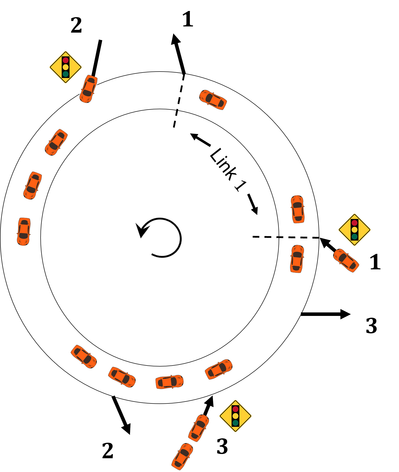
(a)

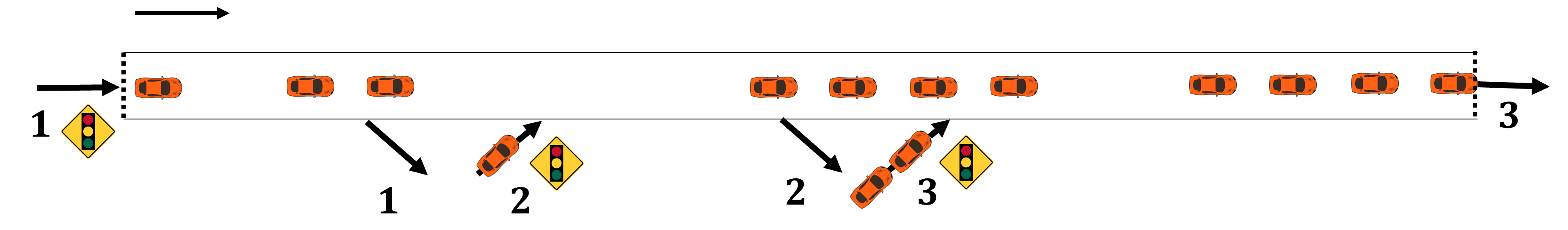
(b)

Figure 1: Example of a (a) ring road configuration, (b) straight road configuration where the traffic light at the upstream entry point indicates that we have control over any previous on-ramp.

3.1 Vehicle Following Safety Constraints

We consider vehicles of length $L$ that have the same acceleration and braking capabilities, and are equipped with V2I communication systems. We use the term ego vehicle to refer to a specific vehicle under consideration, and denote it by $e$. Consider a vehicle following scenario and let $v_{e}$ (resp. $v_{l}$) be the speed of the ego vehicle (resp. its leading vehicle), and $S_{e}$ be the safety distance between the two vehicles required to avoid collision. We assume that $S_{e}$ satisfies

$$S_{e}=hv_{e}+S_{0}+\frac{v^{2}_{e}-v^{2}_{l}}{2|a_{\min}|},$$ (1)

which is calculated based on an emergency stopping scenario with details given in Ioannou and Chien, (1993). Here, $h>0$ is known as the safe time headway constant, $S_{0}>0$ is an additional constant distance, and $a_{\min}<0$ is the minimum possible deceleration of the leading vehicle. For simplicity, we assume a third-order vehicle dynamics throughout the paper. We consider two general modes of operation for each vehicle: the speed tracking mode and the safety mode. The main objective in the speed tracking mode is to adjust the speed to the free flow speed $V_{f}$ when the ego vehicle is far from any leading vehicle; see Appendix A.1. The main objective in the safety mode is to avoid collision when the ego vehicle gets close to a leading vehicle by maintaining the safety distance given by (1). We let $x_{e}=(p_{e},v_{e},a_{e},I_{e})$ be the state of the ego vehicle, where $p_{e}$ is its location, $v_{e}$ is the speed, $a_{e}$ is the acceleration, and $I_{e}$ is a binary variable which is equal to one if the ego vehicle is in the safety mode, and zero otherwise.

Consider an ego vehicle that starts from rest at a ramp meter and remains in the speed tracking mode. We define the acceleration lane of an on-ramp as the section starting from its ramp meter up to the point on the mainline where the ego vehicle reaches the speed $V_{f}$. Note that the acceleration lane may overlap with the mainline if the length of the on-ramp, from the ramp meter to the merging point, is not sufficiently long; see Figure 2. However, if the on-ramp is sufficiently long, then the acceleration lane ends at the merging point where the ego vehicle enters the freeway. We assume that all the vehicles entering the freeway from an on-ramp merge at a fixed merging point. We define the merging speed of an on-ramp as the speed of the ego vehicle at the merging point, assuming that it remains in the speed tracking mode between release and reaching the merging point. Note that the merging speed at an on-ramp is at most $V_{f}$.

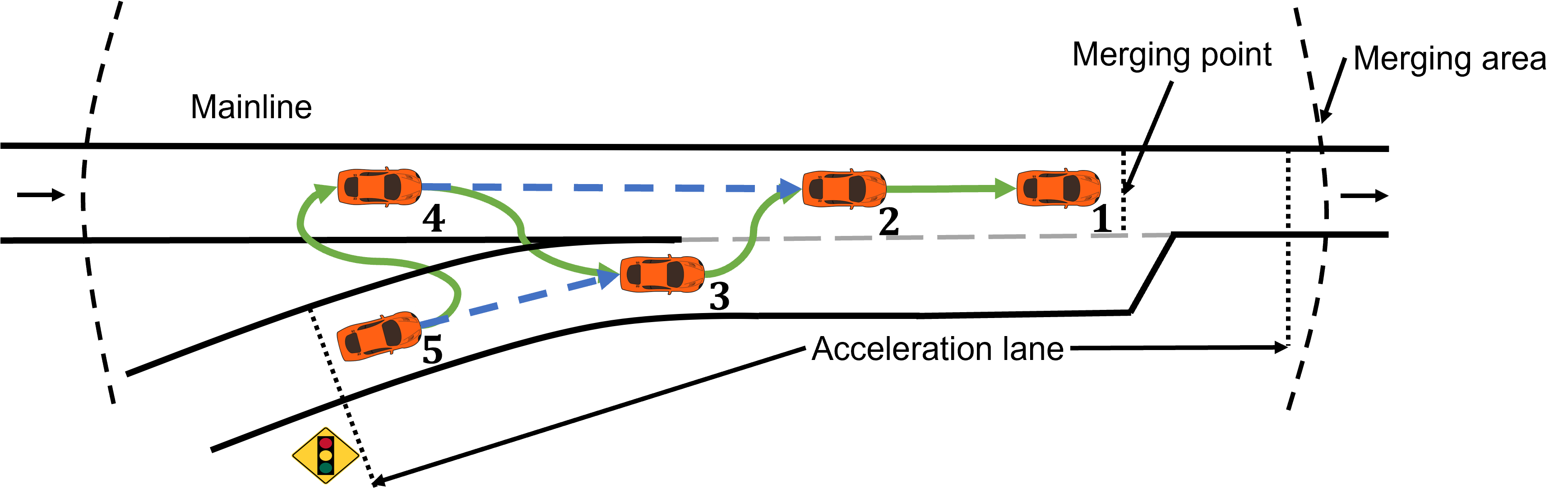
Figure 2: A merging scenario. For each vehicle, the dotted arrow indicates its leading vehicle while the solid arrow indicates its virtual leading vehicle. Note that vehicle $1$ is both the leading and the virtual leading vehicle of vehicle $2$.

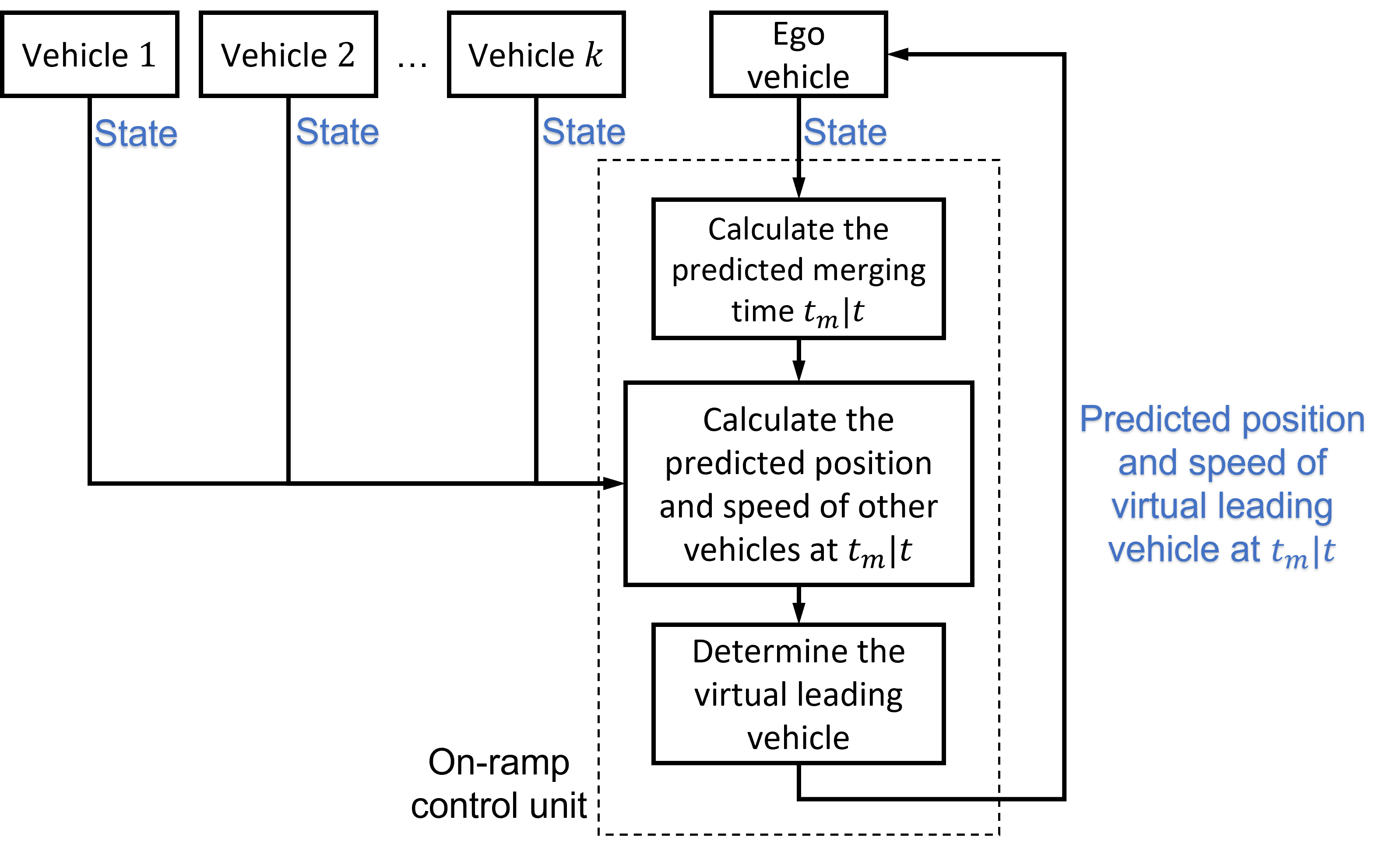
Figure 3: Schematic of the protocol for assigning the ego vehicle’s virtual leading vehicle. Here, $k$ is the number of vehicles, other than the ego vehicle, in the merging area.

Consider a merging scenario as shown in Figure 2. An ego vehicle entering the merging area is assigned a virtual leading vehicle. The virtual leading vehicle, which is the vehicle that is predicted to be in front of the ego vehicle once the ego vehicle has crossed the merging point, is determined (and frequently updated) using a protocol similar to Ntousakis et al., (2016). We will now describe this protocol which is shown in Figure 3. At time $t$, the ego vehicle communicates its state $x_{e}$ to the on-ramp control unit via V2I communication. The on-ramp control unit predicts the time $t_{m}|t$ that the ego vehicle will cross the merging point according to the following prediction rule: if in the speed tracking mode, it assumes that the ego vehicle will remain in this mode in the future; if in the safety mode, it assumes that the ego vehicle will follow a constant speed trajectory in the future. Other vehicles in the merging area also communicate their state to the on-ramp control unit. By using the same prediction rule, the on-ramp control unit predicts the position of each of these vehicles at time $t_{m}|t$, which will determine the ego vehicle’s virtual leading vehicle. Once the virtual leading vehicle has been determined, the on-ramp control unit communicates its predicted position and speed at time $t_{m}|t$ back to the ego vehicle. This information is frequently updated until the ego vehicle has crossed the merging point.

The above protocol describes how a virtual leading vehicle is assigned. The next set of assumptions prescribe the safety rules all the vehicles follow:

• the ego vehicle maintains the constant speed $V_{f}$ at time $t$ if both of the following conditions are satisfied:

  • merging scenario: its predicted distance with respect to its virtual leading vehicle at the moment of merging is safe, i.e.,

    $$\hat{y}_{e}(t_{m}|t)\geq\hat{S}_{e}(t_{m}|t):=h\hat{v}_{e}(t_{m}|t)+S_{0}+\frac{\hat{v}_{e}^{2}(t_{m}|t)-\hat{v}_{\hat{l}}^{2}(t_{m}|t)}{2|a_{\min}|},$$

    where $\hat{y}_{e}(t_{m}|t)$ is the predicted distance between the two vehicles at the moment of merging based on the information available at time $t\leq t_{m}$. Similarly, $\hat{v}_{e}$ and $\hat{v}_{\hat{l}}$ are the predicted speeds of the ego vehicle and its virtual leading vehicle, respectively. These predictions are obtained by the protocol explained above.

  • vehicle following scenario: it is at a safe distance with respect to its leading vehicle, i.e., $y_{e}(t)\geq S_{e}(t)$, where $y_{e}$ is the distance between the two vehicles. Note that if the leading vehicle is also at the constant speed $V_{f}$, then $y_{e}\geq S_{e}=hV_{f}+S_{0}$. This distance is equivalent to a time headway of at least $\tau:=h+(S_{0}+L)/V_{f}$ between the front bumpers of the two vehicles. This rule is widely adopted by human drivers as well as standard adaptive cruise control systems (Ioannou and Chien, (1993)).

• the ego vehicle is initialized to be in the speed tracking mode upon release from the on-ramp. It changes mode at time $t$ if $\hat{y}_{e}(t_{m}|t)<\hat{S}_{e}(t_{m}|t)$ in a merging scenario or $y_{e}(t)<S_{e}(t)$ in a vehicle following scenario. Moreover, if the ego vehicle is released from the on-ramp at least $\tau$ seconds after its leading vehicle, then it will not change mode because of its leading vehicle while the leading vehicle is in the speed tracking mode. Note that the ego vehicle may still change mode because of a virtual leading vehicle.

Note that in order to keep the results fairly general, we intentionally have not specified the total number of submodes within the safety mode, the exact control logic within each submode, or the exact logic for switching back to the speed tracking mode. Such details will be introduced only if and when needed for performance analysis of RM policies in the paper. Also, note that the control logic in the safety mode is allowed to be different for different vehicles when they are not moving at the speed $V_{f}$. However, the following assumption rules out any impractical control logic such as unnecessary braking:

• there exists $T_{\text{free}}$ such that for any initial condition, vehicles reach the free flow state after at most $T_{\text{free}}$ seconds if no other vehicle is released from the on-ramps. The free flow state refers to a state where: (i) if a vehicle is in the safety mode, then it moves at the constant speed $V_{f}$ and will maintain this speed until it exits the network, and (ii) if a vehicle is in the speed tracking mode, then it will remain in this mode until it exits the network.

Example 1.

We present a numerical example to better understand some of the previous assumptions. Let $h=1.5\leavevmode\nobreak\ [\text{sec}]$, $S_{0}=4\leavevmode\nobreak\ [\text{m}]$, $L=4.5\leavevmode\nobreak\ [\text{m}]$, and $V_{f}=15\leavevmode\nobreak\ [\text{m/sec}]$. Suppose that all the vehicles in Figure 2 are moving at the constant speed $V_{f}$ at time $t$, and recall that the safety distance at the free flow speed is $hV_{f}+S_{0}=26.5\leavevmode\nobreak\ [\text{m}]$. Let vehicles $1$-$5$ be $5$, $36$, $70$, $101$, and $132$ meters upstream of the merging point, respectively. Vehicle $3$ (the ego vehicle)’s predicted time of crossing the merging point is $t_{m}|t=70/15=4.67\leavevmode\nobreak\ [\text{sec}]$. The predicted positions of vehicles $1$ and $2$ at time $t_{m}|t$ are $65$ and $34$ meters downstream, and the predicted positions of vehicles $4$ and $5$ at time $t_{m}|t$ are $31$ and $61$ meters upstream of the merging point, respectively. Thus, the ego vehicle’s virtual leading vehicle at time $t_{m}|t$ is determined to be vehicle $2$. Moreover, since $\hat{y}_{e}(t_{m}|t)=34-L=29.5>26.5=\hat{S}_{e}(t_{m}|t)=h\hat{v}_{e}(t_{m}|t)+S_{0}$, the ego vehicle maintains the constant speed $V_{f}$ by (VC1)(a). Similar calculations show that all the other vehicles also maintain their speeds at $V_{f}$.

3.2 Demand Model and Throughput

It will be convenient for performance analysis later on to adopt a discrete time setting. Let the duration of each time step be $\tau=h+(S_{0}+L)/V_{f}$, representing the minimum time headway between the front bumpers of two vehicles that are moving at the speed $V_{f}$ and are at a safe distance; see (VC1)(b) in Section 3.1. We assume that vehicles arrive to on-ramp $i\in[m]$ according to an i.i.d. Bernoulli process with parameter $\lambda_{i}\in[0,1]$ independent of the other on-ramps. That is, in any given time step, the probability that a vehicle arrives at the $i$-th on-ramp is $\lambda_{i}$ independent of everything else. Note that $\lambda_{i}$ specifies the arrival rate to on-ramp $i$ in terms of the number of vehicles per $\tau$ seconds. Let $\lambda:=[\lambda_{i}]$ be the vector of arrival rates. The destination off-ramp for individual arriving vehicles is assumed to be i.i.d. and given by the routing matrix $R=[R_{ij}]$, where $0\leq R_{ij}\leq 1$ is the probability that a vehicle arriving to on-ramp $i$ wants to exit from off-ramp $j$. Note that $R_{ij}$ specifies the long-run fraction of arrivals at on-ramp $i$ that want to exit from off-ramp $j$. Naturally, for every on-ramp $i$ we have $\sum_{j}R_{ij}=1$. Finally, we let $\tilde{R}=[\tilde{R}_{ij}]$ be the cumulative routing matrix, where $\tilde{R}_{ij}$ is the fraction of arrivals at on-ramp $i$ that need to use link $j$ in order to reach their destination. Therefore, $\lambda_{i}\tilde{R}_{ij}$ is the rate of arrivals at on-ramp $i$ that need to use link $j$ in order to reach their destination, i.e., the load induced on link $j$ by on-ramp $i$. Let $\rho_{j}:=\sum_{i}\lambda_{i}\tilde{R}_{ij}$ be the total load induced on link $j$ by all the on-ramps, and let $\rho:=\max_{j\in[m]}\rho_{j}$ be the maximum load.

Remark 1.

The current demand model, i.e., Bernoulli arrivals and Bernoulli routing, is chosen to simplify the technical details in the proofs. We believe that our results are far more general and hold for more practical demand models used in the literature, e.g., see Jin et al., (2009) for an example of arrival models.

Example 2.

Let the number of on- and off-ramps be $m=3$, and let the routing matrix be

$$R=\begin{pmatrix}R_{11}&R_{12}&R_{13}\\ R_{21}&R_{22}&R_{23}\\ R_{31}&R_{32}&R_{33}\end{pmatrix}.$$

Then, the cumulative routing matrix is

$$\tilde{R}=\begin{pmatrix}1&1-R_{11}&1-(R_{11}+R_{12})\\ 1-(R_{22}+R_{23})&1&1-R_{22}\\ 1-R_{33}&1-(R_{31}+R_{33})&1\end{pmatrix}=\begin{pmatrix}1&R_{12}+R_{13}&R_{13}\\ R_{21}&1&R_{21}+R_{23}\\ R_{31}+R_{32}&R_{32}&1\end{pmatrix}.$$

We now formalize the notion of “throughput" which is the key performance metric in this paper. Let $Q_{i}(t)$ be the queue size at on-ramp $i\in[m]$, and $Q(t)=[Q_{i}(t)]$ be the vector of queue sizes at time $t$. For a given routing matrix $R$, the under-saturation region of a RM policy $\pi$ is defined as follows:

$$U_{\pi,R}=\{\lambda:\limsup_{t\to\infty}\mathbb{E}\left[Q_{i}(t)\right]<\infty\leavevmode\nobreak\ \leavevmode\nobreak\ \forall i\in[m]\leavevmode\nobreak\ \text{under policy}\leavevmode\nobreak\ \pi\}.$$

This is the set of $\lambda$’s for which the queue sizes at all the on-ramps remain bounded in expectation. The boundary of this set is called the throughput of the policy $\pi$. We are interested in finding a RM policy $\pi$ such that for every $R$, $U_{\pi^{\prime},R}\subseteq U_{\pi,R}$ for all policies $\pi^{\prime}$, including those that have prior knowledge of $\lambda$ and $R$. In other words, for every $R$, if the freeway remains under-saturated under some policy $\pi^{\prime}$, then it also remains under-saturated under the policy $\pi$. In that case, we say that policy $\pi$ maximizes the throughput. One of our main contributions is designing policies that are reactive, i.e., they do not require $\lambda$ and $R$, but maximize throughput for all practical purposes.

Remark 2.

A rigorous definition of the throughput should also include its dependence on the initial condition of the vehicles and the initial queue sizes. We have removed this dependence for simplicity since the throughput of our policies do not depend on the initial condition.

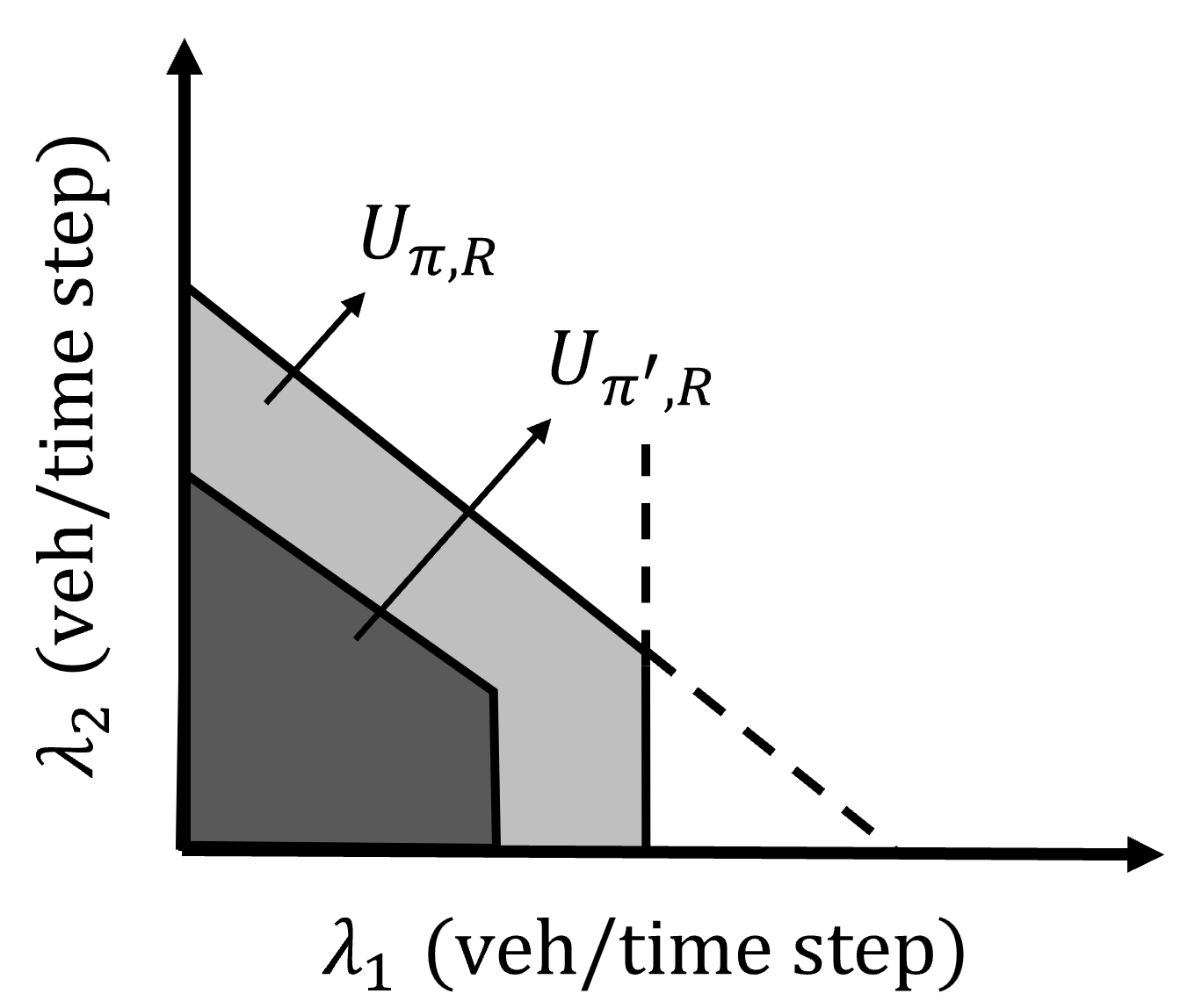
Figure 4: An illustration of the under-saturation region of some policy $\pi^{\prime}$ (dark grey area) and a policy $\pi$ that maximizes the throughput (dark + light grey areas).

Example 3.

Let $m=3$ and consider a given $R$. Suppose that a policy $\pi$ is able to maximize the throughput; that is, for any other policy $\pi^{\prime}$, we have $U_{\pi^{\prime},R}\subseteq U_{\pi,R}$. An illustration of $U_{\pi,R}$ and $U_{\pi^{\prime},R}$ is shown in Figure 4 for a fixed $\lambda_{3}$. From the figure, one can see that if $(\lambda_{1},\lambda_{2})\in U_{\pi^{\prime},R}$, then $(\lambda_{1},\lambda_{2})\in U_{\pi,R}$, i.e., if the freeway remains under-saturated under the policy $\pi^{\prime}$, then it also remains under-saturated under the policy $\pi$. We will provide a numerical characterization of $U_{\pi,R}$ in Example 6.

3.3 Slot

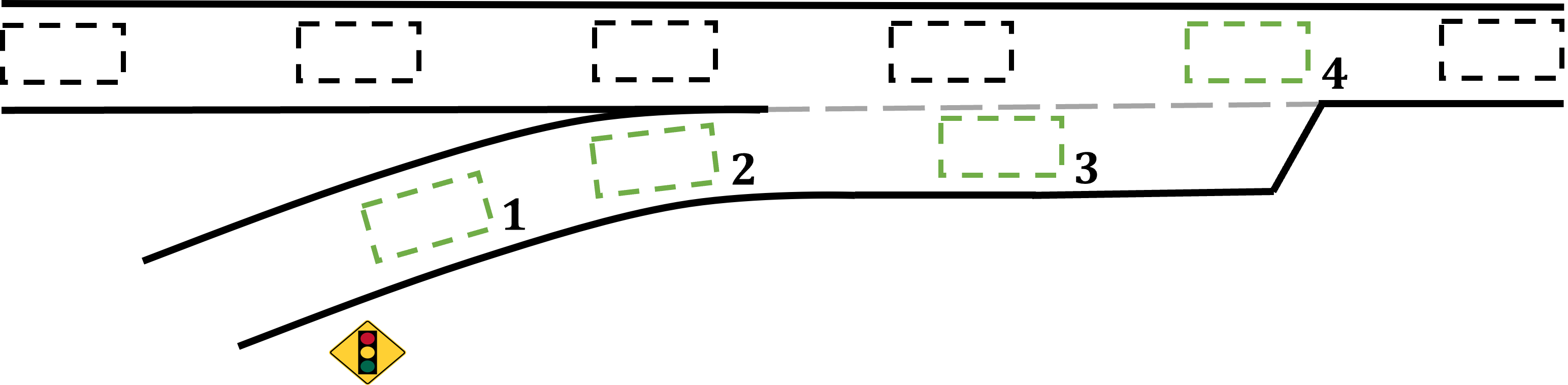
Figure 5: A configuration of slots for the mainline and acceleration lane of an on-ramp. There are four slots for the acceleration lane (colored in green) with slot $4$ coinciding with a mainline slot.

To conveniently track vehicle locations in discrete time, we introduce the notion of slot. A slot corresponds to a specific point on either the mainline or acceleration lanes at a given time. We first define the mainline slots. Let $n_{c}$ denote the maximum number of distinct points that can be placed on the mainline, such that the distance between adjacent points is $hV_{f}+S_{0}+L$. This distance is governed by the safety distance $S_{e}$, as explained in Section 3.1. In other words, $n_{c}$ is the maximum number of vehicles that can move at the speed $V_{f}$ on the mainline without violating the vehicle following safety constraints. Consider a configuration of these $n_{c}$ points at time $t=0$. Each point represents a slot on the mainline that moves at the free flow speed. Without loss of generality, we assume that the length of the mainline $P$ is such that each slot replaces the next slot at the end of each time step.

Next, we define the acceleration lane slots. Consider the $i$-th on-ramp and suppose that an ego vehicle starts from rest at its ramp meter and remains in the speed tracking mode. At the end of each time step, the ego vehicle’s location represents a slot for the acceleration lane of on-ramp $i$. These slots continue until the ego vehicle exits the acceleration lane. For example, if the ego vehicle exits the acceleration after $3.5\tau$ seconds, there are four slots corresponding to its location at times $\tau$, $2\tau$, $3\tau$, and $4\tau$; see Figure 5. Let $n_{i}$ be the number of slots for the acceleration lane of on-ramp $i$, and $n_{a}=\sum_{i}n_{i}$. Note that by definition, the last slot of every acceleration lane is on the mainline. Without loss of generality, we consider a configuration of slots at $t=0$, such that the last slot of every acceleration lane coincides with a mainline slot. The details to justify the no loss in generality are given as follows: for a given configuration of mainline slots at $t=0$, there exists $t_{i}\in[0,\tau)$ such that the last acceleration lane slot of on-ramp $i$ coincides with a mainline slot at time $t_{i}$. Thereafter, the last acceleration lane slot coincides with a mainline slot after every $\tau$ seconds, i.e., at times $k\tau+t_{i}$ for all $k\in\mathbb{N}_{0}$. The times $k\tau+t_{i}$, $k\in\mathbb{N}_{0}$, are the release times of on-ramp $i$ in the proposed RM policies. Therefore, the assumption that all the last acceleration lane slots initially coincide with a mainline slot (which corresponds to $t_{i}=0$ for all $i\in[m]$) only means a shifted sequence of release times, which justifies the no loss in generality.

Consider an initial condition of the vehicles, where the vehicles are in the free flow state and the location of each vehicle coincides with a slot for all times in the future. For this initial condition and under the proposed RM policies, the following sequence of events occurs during each time step: (i) the mainline slots rotate one position in the direction of travel and replace the next slot. Similarly, the acceleration lane slots of each on-ramp replace the next slot, with the last slot replacing the first slot. The numbering of the slots is reset, with the new first mainline slot after on-ramp $1$ numbered $1$, and the rest of the mainline slots numbered in an increasing order; the acceleration lane slots are numbered similarly; (ii) vehicles that reach their destination off-ramp exit the network without creating any obstruction for the upstream vehicles; (iii) if permitted by the RM policy, a new vehicle is released. For the given initial condition and under the proposed RM policies, the location of the newly released vehicle will coincide with a slot for all times in the future .

4 Ramp Metering and Performance Analysis

In this section, we present traffic-responsive RM policies that operate under vehicle following safety constraints and analyze their performance. An inner-estimate to the under-saturation region of each policy is provided in Sections 4.1-4.5, and is then compared to an outer-estimate in Section 4.6. In Section 4.7, we discuss the extension of our results to the straight road configuration.

For easier navigation, we briefly review the proposed policies here. The policies in Sections 4.1, 4.2, and 4.4 are coordinated, while the one in Section 4.3 is a distributed version of the coordinated policy in Section 4.2, and the one in Section 4.5 is a local policy. All of the proposed policies operate under vehicle following safety constraints, where the on-ramps release new vehicles only if there is sufficient gap between vehicles on the mainline at the moment of release. Moreover, All of the policies are reactive, meaning that they only require real-time traffic measurements without requiring any prior knowledge of the arrival rate $\lambda$ or the routing matrix $R$. They obtain the real-time traffic measurements by V2I communication.

The proposed RM policies work in synchronous cycles during which an on-ramp does not release more vehicles than the number of vehicles waiting in its queue, i.e., its queue size, at the start of the cycle. The synchronization of cycles is done in real time in Section 4.1, whereas it is done once offline in Sections 4.2-4.5. The policies differ in how they use the traffic measurements: (i) the policy in Section 4.1 pauses release until a new cycle starts, (ii) the policies in Sections 4.2-4.3 adjust the time between successive releases during a cycle, and (iii) the policy in Section 4.4 adopts a conservative dynamic safe gap criterion for release during a cycle. However, the actions of the three policies in Sections 4.2-4.4 at the free flow state are equivalent to that of the local policy in Section 4.5.

The traffic measurements required by the proposed policies will be a combination of $Q$ and the state (or part of the state) of all the vehicles $X:=(x_{e})_{e\in[n]}$. Here, $n$ is the number of vehicles on the mainline and acceleration lanes, and $x_{e}$ is the state of the ego vehicle as defined in Section 3.1. These measurements are communicated to the on-ramps by V2I communication. Table 2 provides a summary of the communication cost of the RM policies considered in this paper. The notion of communication cost is explained in Appendix A.2. In Table 2, $n_{m}$ is the total number of slots in all the merging areas, which is at most $n_{c}+n_{a}$, $T_{\text{per}}$ is a design update period, and $c_{i}$, $i=1,2$, is the contribution of the queue size to the communication cost.

Section	RM Policy		Worst-case Communication Cost
			(number of transmissions per $\tau$ seconds)
4.1	Renewal		$n_{c}+n_{a}+c_{1}$
4.2	Dynamic Release Rate (DRR)		$m(n_{c}+n_{a})/T_{\text{per}}+n_{m}+c_{2}$
4.3	Distributed DRR (DisDRR)		$(n_{c}+n_{a})/T_{\text{per}}+n_{m}+c_{2}$
4.4	Dynamic Space Gap (DSG)		$(n_{c}+n_{a})m+c_{2}$
4.5	Greedy		$n_{m}$

Table 2: Summary of the RM policies studied in this paper.

4.1 Renewal Policy

The first policy, called the Renewal policy, is inspired by the queuing theory literature in the context of communication networks, e.g., see Georgiadis et al., (1995); Armony and Bambos, (2003). In this policy, an on-ramp pauses vehicle release once it has released all the vehicles waiting at the start of a cycle until all other on-ramps have done the same.

Definition 1.

(Renewal ramp metering policy) No vehicle is released until all the initial vehicles reach the free flow state, as defined in (VC3), at time $t_{1}$. Thereafter, the policy works in cycles of variable length. At the start of the $k$-th cycle at time $t_{k}$, each on-ramp allocates itself a “quota" equal to the number of vehicles at that on-ramp at $t_{k}$. At time $t$ during the cycle, an on-ramp releases the ego vehicle if the following conditions are satisfied:

• $t=k\tau$ for some $k\in\mathbb{N}_{0}$.

• the on-ramp has not reached its quota.

• $y_{e}(t)\geq S_{e}(t)$, i.e., the ego is at a safe distance with respect to its leading vehicle (cf. (VC1)(b)).

• it predicts that the ego vehicle will be at a safe distance with respect to its virtual leading and following vehicles between merging and exiting the acceleration lane (cf. (VC1)(a)).

Once an on-ramp reaches its quota, it pauses vehicle release until all other on-ramps reach their quotas, at which point the next cycle starts.

Remark 3.

A simpler form of this policy, called the Quota policy, is analyzed in Georgiadis et al., (1995). In order to apply the Quota policy directly to the current transportation setting, additional analysis is required that considers the vehicle dynamics. This analysis is done in the next theorem.

We introduce an additional notation for the next result. Consider a situation where on-ramp $i$ releases the ego vehicle under (M1)-(M4), and its virtual leading and following vehicles are moving at the speed $V_{f}$, both occupying mainline slots. We let $\tau_{i}$ be the minimum time headway between the front bumpers of the virtual leading and following vehicles, ensuring that they maintain a safe distance from the ego vehicle after merging. Note that since both the virtual leading and following vehicles are assumed to occupy mainline slots, $\tau_{i}$ is an exact multiple of $\tau$ and $\tau_{i}\geq 2\tau$, where the equality holds if and only if the merging speed at on-ramp $i$ is $V_{f}$.

Theorem 1.

For any initial condition, the Renewal policy keeps the freeway under-saturated if $(\frac{\tau_{i}}{\tau}-1)\rho_{i}-(\frac{\tau_{i}}{\tau}-2)\lambda_{i}<1$ for all $i\in[m]$.

Proof.

See Appendix C.1. ∎

V2I communication requirements: the Renewal policy requires the vector queue sizes $Q=[Q_{i}(t)]$ and the state of all the vehicles $X$. Its worst-case communication cost is calculated as follows: at each time step during a cycle, any vehicle that is on the mainline or an acceleration lane must communicate its state to all on-ramps. This information is used both for safety distance evaluation (cf. (M3)-(M4)) and verifying that the vehicles are in the free flow state. After a finite time, the number of vehicles that communicate their state is no more than $n_{c}+n_{a}$. Furthermore, at the start of every cycle, all the vehicles in each on-ramp queue must communicate their presence in the queue to that on-ramp. The contribution of the on-ramp queue to the communication cost is

$$c_{1}:=\limsup_{K\rightarrow\infty}\frac{1}{K}\sum_{t_{k}\leq K\tau}\sum_{i\in[m]}Q_{i}(t_{k}),$$

where $t_{k}$ is the start of the $k$-th cycle in the Renewal policy. Hence, the communication cost $C$ is upper-bounded by $n_{c}+n_{a}+c_{1}$ transmissions per $\tau$ seconds.

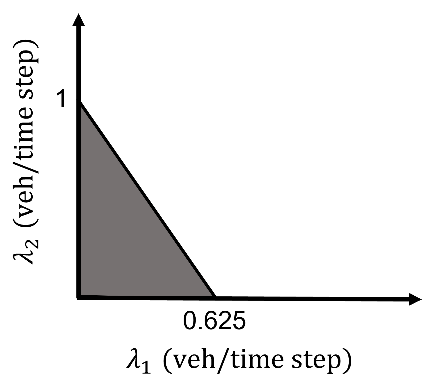
Figure 6: An inner-estimate of the under-saturation region of the Renewal policy (grey area) from Example 4.

Remark 4.

Under the constant time headway safety distance rule in Section 3.1, the flow capacity of the mainline is $1$ vehicle per $\tau$ seconds. Theorem 1 provides an inner-estimate of the under-saturation region in terms of the induced loads $\rho_{i}$, arrival rates $\lambda_{i}$, and the mainline flow capacity. In particular, if for every $i\in[m]$, $(\tau_{i}/\tau-1)\rho_{i}-(\tau_{i}/\tau-2)\lambda_{i}$ is less than the flow capacity, then the Renewal policy keeps the freeway under-saturated.

Example 4.

Let $m=3$ and suppose that $\tau_{1}=\tau_{3}=2\tau$, $\tau_{2}=3\tau$, i.e., the merging speed at on-ramps $1$ and $3$ are $V_{f}$ and is lower at on-ramp $2$. Let

$$R=\begin{pmatrix}0.2&0.7&0.1\\ 0&0.8&0.2\\ 0.5&0&0.5\end{pmatrix},\leavevmode\nobreak\ \lambda_{3}=0.5\leavevmode\nobreak\ [\text{veh}/\text{time step}].$$

Then, the inner-estimate of the under-saturation region given by Theorem 1 is

$$\{(\lambda_{1},\lambda_{2}):\rho_{1}<1,\leavevmode\nobreak\ 2\rho_{2}-\lambda_{2}<1,\leavevmode\nobreak\ \rho_{3}<1\} =\{(\lambda_{1},\lambda_{2}):\lambda_{1}+0.5\lambda_{2}<1,\leavevmode\nobreak\ 1.6\lambda_{1}+\lambda_{2}<1,\leavevmode\nobreak\ 0.1\lambda_{1}+0.2\lambda_{2}<1\}$$

$$=\{(\lambda_{1},\lambda_{2}):1.6\lambda_{1}+\lambda_{2}<1\},$$

which is illustrated in Figure 6.

Recall that one of our contributions is understanding the interplay of safety and throughput. This interplay is captured using the parameter $\tau_{i}$, $i\in[m]$. In particular, as the merging speed at an on-ramp decreases, the required safety distance $S_{e}$ in (1) increases, which would increase $\tau_{i}$. This puts a limit on the rate at which the on-ramp can release new vehicles under the vehicle following safety constraint, which in turn decreases the throughput.

Remark 5.

The Renewal policy has a variable cycle length that depends on queue sizes at the start of the cycle, with larger queue sizes generally leading to longer cycles. The impact of a variable cycle length on performance can be both positive and negative. On one hand, it can increase the total travel time because, any arrival during a cycle is delayed until the next cycle starts. To avoid this issue, one may enforce a fixed cycle length (independent of the queue sizes). However, this could have a negative impact on throughput. In particular, a variable cycle length increases the chance of vehicles being released in platoons, rather than individually. Such a platoon release can be more efficient in using the space on the freeway since it can increase the release rate of the on-ramps, thus improving the throughput. For example, let the merging speed at on-ramp $i$ be less than $V_{f}$ such that $\tau_{i}=3\tau$ seconds, and suppose that two vehicles are waiting in on-ramp $i$’s queue. Each vehicle requires a time headway of at least $\tau_{i}$ seconds between the mainline vehicles to safely merge between them. Therefore, the individual release requires a time headway of $2\tau_{i}=6\tau$ seconds in total. However, the platoon release only requires a time headway of $\tau_{i}+\tau=4\tau$ seconds. As we will show, this phenomenon can result in a better throughput under the Renewal policy compared to the other policies in the paper which use a fixed cycle length.

4.2 Dynamic Release Rate Policy

This policy imposes dynamic minimum time gap criterion, in addition to (M1), between release of successive vehicles from the same on-ramp. Changing the time gap between release of successive vehicles by an on-ramp is similar to changing its release rate, and hence the name of the policy.

Definition 2.

(Dynamic Release Rate (DRR) ramp metering policy) The policy works in cycles of fixed length $T_{\text{cyc}}\tau$, where $T_{\text{cyc}}\in\mathbb{N}$. At the start of the $k$-th cycle at $t_{k}=(k-1)T_{\text{cyc}}\tau$, each on-ramp allocates itself a “quota" equal to the number of vehicles at that on-ramp at $t_{k}$. At time $t\in[t_{k},t_{k+1}]$ during the $k$-th cycle, on-ramp $i$ releases the ego vehicle if (M1)-(M4) and the following condition are satisfied:

• at least $g(t)$ seconds has passed since the release of the last vehicle from on-ramp $i$, where $g(t)$ is a piecewise constant minimum time gap, updated periodically at $t=T_{\text{per}},2T_{\text{per}},\ldots$, as described in Algorithm 1.

Once an on-ramp reaches its quota, it pauses release during the rest of the cycle.

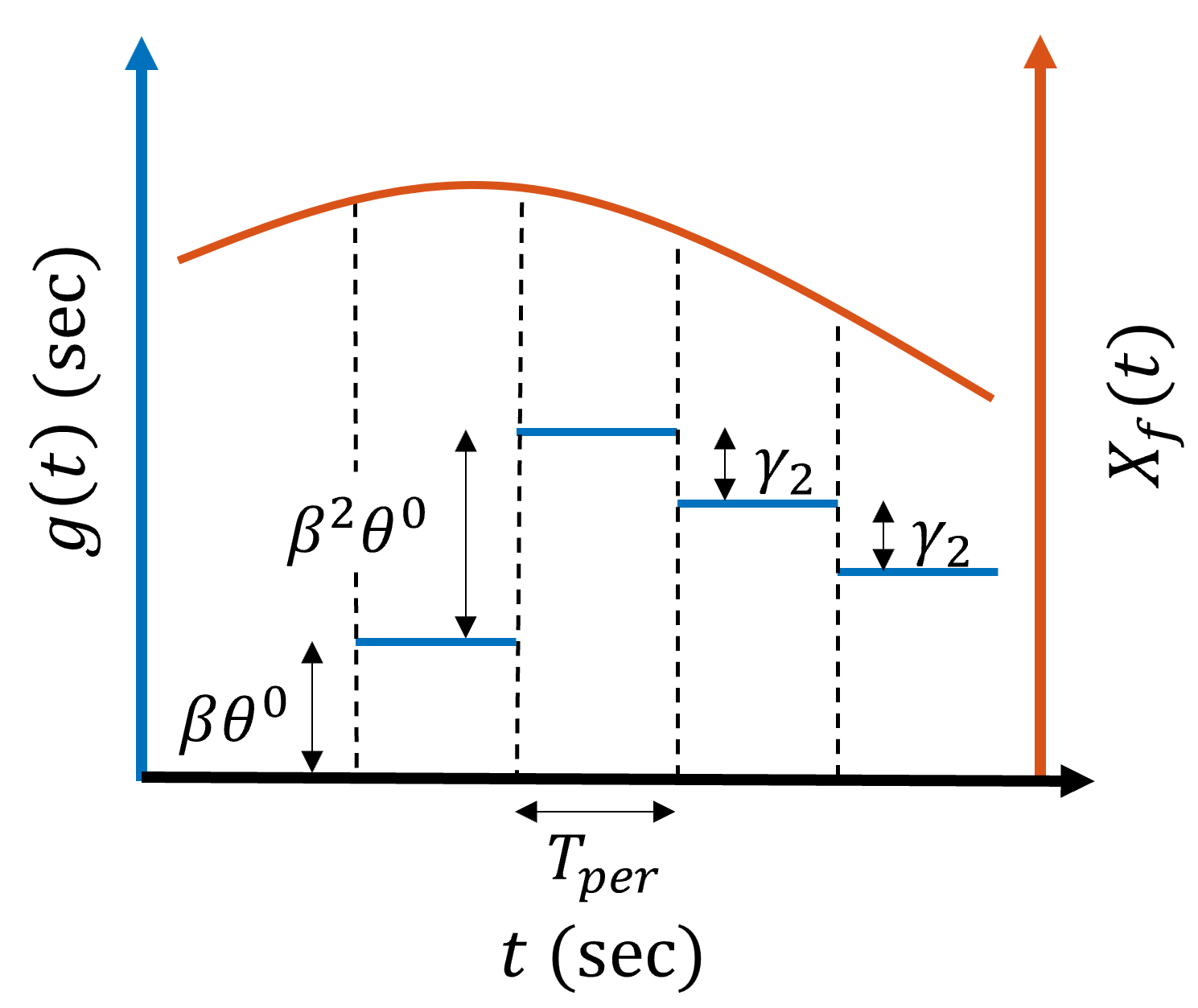
Figure 7: An illustration of the update rule for the minimum time gap $g$ in Algorithm 1.

Algorithm 1 Update rule for the minimum time gap between release of vehicles under the DRR policy

design constants: $T_{\text{per}}>0,\gamma_{1}>0$, $\gamma_{2}>0$, $\theta^{\circ}>0$, $\beta>1$  initial condition:  $g(0)=0,\leavevmode\nobreak\ \theta(0)=\theta^{\circ}$, $X_{f}(0)=X_{f_{1}}(0)$ for $t=T_{\text{per}},2T_{\text{per}},\cdots$ do

if $X_{f}(t)\leq\max\{X_{f}(t-T_{\text{per}})-\gamma_{1}{},0\}$  then

     $\theta(t)\leftarrow\theta(t-T_{\text{per}})$

     $g(t)\leftarrow\max\{g(t-T_{\text{per}})-\gamma_{2},0\}$

else

     $\theta(t)\leftarrow\beta\theta(t-T_{\text{per}})$

     $g(t)\leftarrow g(t-T_{\text{per}})+\theta(t)$

end if end for

In Algorithm 1, $X_{f}(t):=X_{f_{1}}(t)+X_{f_{2}}(t)$, where $X_{f_{1}}$ and $X_{f_{2}}$ are defined as follows: $X_{f_{1}}(t):=\sum_{e\in[n]}(w_{1}|v_{e}(t)-V_{f}|+w_{2}|a_{e}(t)|)I_{e}(t)$, where $n$ is the number of vehicles on the mainline and acceleration lanes, and $w_{1},w_{2}$ are normalization factors. Furthermore, for $t\geq T_{\text{per}}$, $X_{f_{2}}(t):=\sum w_{3}(\delta_{e}(t)+\hat{\delta}_{e}(t))$, where $w_{3}$ is a normalization factor and the sum is over all the vehicles that either have: (i) violated the safety distance $S_{e}$ at some time in $[t-T_{\text{per}},t]$, or (ii) predicted at some time in $[t-T_{\text{per}},t]$ that they would violate the safety distance once they reach a merging point. The terms $\delta_{e}$ and $\hat{\delta}_{e}$ are, respectively, the maximum error and maximum predicted error in the relative spacing, and are given by

$$\delta_{e}(t) =\max_{t^{\prime}\in[t-T_{\text{per}},t]}|y_{e}(t^{\prime})-S_{e}(t^{\prime})|\mathbbm{1}_{\{y_{e}(t^{\prime})<S_{e}(t^{\prime})\}},$$

$$\hat{\delta}_{e}(t) =\max_{t^{\prime}\in[t-T_{\text{per}},t]}|\hat{y}_{e}(t_{m}|t^{\prime})-\hat{S}_{e}(t_{m}|t^{\prime})|\mathbbm{1}_{\{\hat{y}_{e}(t_{m}|t^{\prime})<\hat{S}_{e}(t_{m}|t^{\prime})\}},$$

where $\mathbbm{1}$ is the indicator function, and $t_{m}|t^{\prime}$ is the predicted time of crossing a merging point based on the information available at time $t^{\prime}\leq t_{m}$. If $\delta_{e}+\hat{\delta}_{e}$ is non-zero, then the ego vehicle communicates it either right before leaving the network, or at the update times $T_{\text{per}},2T_{\text{per}},\ldots$, whichever comes earlier. Otherwise, it is not communicated by the ego vehicle.

Remark 6.

Recall the safety distance $S_{e}$ in (1). Since the speeds of the vehicles are bounded, $S_{e}$ is also bounded. Hence, $\delta_{e}$ and $\hat{\delta}_{e}$ in $X_{f_{2}}$ are bounded. We use this in the proof of the next result.

Theorem 2.

For any initial condition, $T_{\text{cyc}}\in\mathbb{N}$, and design constants in Algorithm 1, the DRR policy keeps the freeway under-saturated if $(\frac{\tau_{i}}{\tau}-1)\rho_{i}<1$ for all $i\in[m]$.

Proof.

See Appendix C.2. ∎

V2I communication requirements: The DRR policy requires the vector queue sizes $Q=[Q_{i}(t)]$ (if $T_{\text{cyc}}>1$) and the state of all the vehicles $X$. Its worst-case communication cost is calculated as follows: after a finite time, $X$ is communicated to all on-ramps only at the end of each update period $T_{\text{per}}$. After such finite time, the number of vehicles that constitute $X$ is no more than $n_{c}+n_{a}$. Furthermore, at each time step during a cycle, the vehicles in the merging area of each on-ramp communicate their state to that on-ramp for safety distance evaluation (cf. (M3)-(M4)). The number of vehicles in all the merging areas is at most $n_{m}$. Finally, if $T_{\text{cyc}}>1$, then all the vehicles in each on-ramp queue must communicate their presence in the queue to that on-ramp at the start of every cycle. The contribution of the queue size to the communication cost is

$$c_{2}:=\left(\limsup_{K\rightarrow\infty}\frac{1}{K}\sum_{k\leq K/T_{\text{cyc}}+1}\sum_{i\in[m]}Q_{i}((k-1)T_{\text{cyc}}\tau)\right)\mathbbm{1}_{\{T_{\text{cyc}}>1\}}.$$

Hence, $C$ is upper bounded by $m(n_{c}+n_{a})/T_{\text{per}}+n_{m}+c_{2}$ transmissions per $\tau$ seconds.

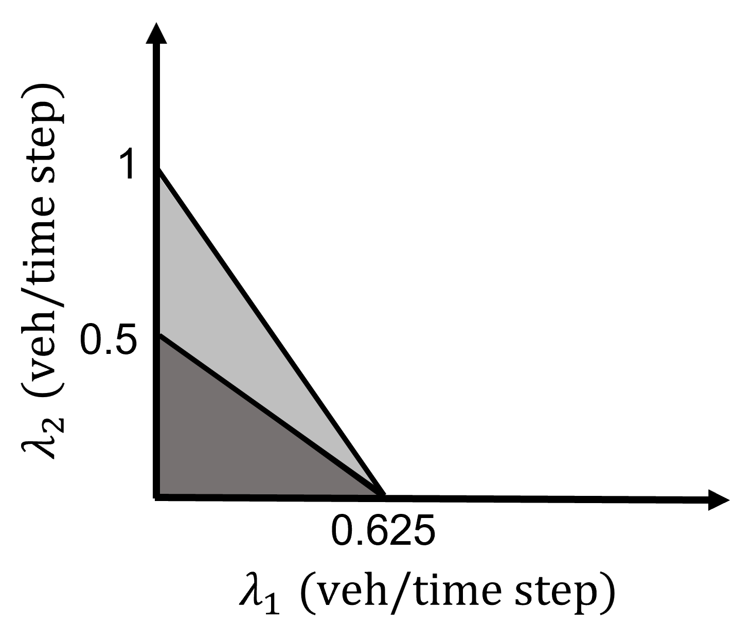
Figure 8: An inner-estimate of the under-saturation region (dark grey area) of the DRR policy from Example 5. The light grey area indicates the additional under-saturation region if we use the Renewal policy.

Remark 7.

Similar to Theorem 1, Theorem 2 provides an inner-estimate of the under-saturation region of the DRR policy in terms of the induced loads $\rho_{i}$ and the mainline flow capacity. The region specified by this estimate is the same for all $T_{\text{cyc}}\in\mathbb{N}$ and is contained in the one given for the Renewal policy in Theorem 1. However, this does not necessarily mean that the throughput of the DRR policy is the same for different cycle lengths, or the Renewal policy gives a better throughput as the inner-estimates may not be exact. A simulation comparison of the throughput of the DRR policy for different cycle lengths is provided in Section 5.2.

Example 5.

Let the network parameters be as in Example 4. Then, the inner-estimate of the under-saturation region given by Theorem 2 is

$$\{(\lambda_{1},\lambda_{2}):\rho_{1}<1,\leavevmode\nobreak\ 2\rho_{2}<1,\leavevmode\nobreak\ \rho_{3}<1\} =\{(\lambda_{1},\lambda_{2}):\lambda_{1}+0.5\lambda_{2}<1,\leavevmode\nobreak\ 1.6\lambda_{1}+2\lambda_{2}<1,\leavevmode\nobreak\ 0.1\lambda_{1}+0.2\lambda_{2}<1\}$$

$$=\{(\lambda_{1},\lambda_{2}):1.6\lambda_{1}+2\lambda_{2}<1\},$$

which is illustrated in Figure 8 and compared with the inner-estimate of the Renewal policy in Example 4.

The DRR policy is coordinated since each on-ramp requires the state of all the vehicles. The next policy is a distributed version of the DRR policy, where each on-ramp receives information from its downstream on-ramps and the vehicles in its vicinity.

4.3 Distributed Dynamic Release Rate Policy

This policy imposes dynamic minimum time gap criterion, just like its coordinated counterpart. However, each on-ramp only receives information from its downstream on-ramps and the vehicles in its vicinity.

Definition 3.

(Distributed Dynamic Release Rate (DisDRR) ramp metering policy) The policy works in cycles of fixed length $T_{\text{cyc}}\tau$, where $T_{\text{cyc}}\in\mathbb{N}$. At the start of the $k$-th cycle at $t_{k}=(k-1)T_{\text{cyc}}\tau$, each on-ramp allocates itself a “quota" equal to the number of vehicles at that on-ramp at $t_{k}$. At time $t\in[t_{k},t_{k+1}]$ during the $k$-th cycle, on-ramp $i$ releases the ego vehicle if (M1)-(M4) and the following condition are satisfied:

• at least $g_{i}(t)$ seconds has passed since the release of the last vehicle from on-ramp $i$, where $g_{i}(t)$ is a piecewise constant minimum time gap, updated periodically at $t=T_{\text{per}},2T_{\text{per}},\ldots$ according to Algorithm 2.

Once an on-ramp reaches its quota, it pauses release during the rest of the cycle.

Algorithm 2 Update rule for the minimum time gap between release of vehicles under the DisDRR policy

design constants: $T_{\text{per}}>0$, $T_{\text{max}}>0$, $\gamma_{1}>0$, $\gamma_{2}>0$, $\theta_{i}^{\circ}>0$, $\beta>1$  initial condition: $(g_{i}(0),g_{i}(T_{\text{per}}))=(0,0),\leavevmode\nobreak\ (\theta_{i}(0),\theta_{i}(T_{\text{per}}))=(\theta_{i}^{\circ},\theta_{i}^{\circ}),\leavevmode\nobreak\ X_{f}^{i}(0)=X_{f_{1}}^{i}(0),\leavevmode\nobreak\ i\in[m]$ for $t=2T_{\text{per}},3T_{\text{per}},\cdots$ do the following for each on-ramp $i\in[m]$

if $X_{f}^{i}(t)\leq\max\{X_{f}^{i}(t-T_{\text{per}})-\gamma_{1},0\}$ then

     if $g_{i+1}(t-T_{\text{per}})\leq T_{\text{max}}$ or $\sum_{j>i}X_{f}^{j}(t)\leq\max\{\sum_{j>i}X_{f}^{j}(t-T_{\text{per}})-\gamma_{1},0\}$ then

         $\theta_{i}(t)\leftarrow\theta_{i}(t-T_{\text{per}})$

         $g_{i}(t)\leftarrow\max\{g_{i}(t-T_{\text{per}})-\gamma_{2},0\}$

     else

         $\theta_{i}(t)\leftarrow\beta\theta_{i}(t-T_{\text{per}})$

         $g_{i}(t)\leftarrow g_{i}(t-T_{\text{per}})+\theta_{i}(t)$

     end if

else

     if $X_{f}^{i}(t-T_{\text{per}})\leq\max\{X_{f}^{i}(t-2T_{\text{per}})-\gamma_{1},0\}$ then

         $\theta_{i}(t)\leftarrow\beta\theta_{i}(t-T_{\text{per}})$

     else

         $\theta_{i}(t)\leftarrow\theta_{i}(t-T_{\text{per}})$

     end if

     $g_{i}(t)\leftarrow g_{i}(t-T_{\text{per}})+\theta_{i}(t)$

end if end for

For $i\in[m]$, let $X_{f}^{i}$ be the part of $X_{f}$ associated with all the vehicles located between the $i$-th and $(i+1)$-th on-ramps. Thus, $X_{f}=\sum_{i\in[m]}X_{f}^{i}$. We assume that $X_{f}^{i}$ is available to on-ramp $i$. Furthermore, if $g_{i+1}(t)>T_{\text{max}}$ for some design constant $T_{\text{max}}$, then all the on-ramps $j$ downstream of on-ramp $i$ communicate $X_{f}^{j}$ to on-ramp $i$. In that case, $\sum_{j>i}X_{f}^{j}$ is available to on-ramp $i$, where the notation “$j>i$" means that on-ramp $j$ is downstream of on-ramp $i$. Note that for the ring road configuration, all the on-ramps downstream of on-ramp $i$ is the same as all the on-ramps. Hence, $\sum_{j>i}X_{f}^{j}=X_{f}$ for the ring road configuration. Informally, when $g_{i+1}\leq T_{\text{max}}$, $g_{i}$ depends only on the traffic condition in the vicinity of on-ramp $i$, whereas when $g_{i+1}>T_{\text{max}}$, it also depends on the downstream traffic condition. Naturally, higher values of $T_{\text{max}}$ make the policy more “decentralized", but it may take longer to reach the free flow state.

Proposition 1.

For any initial condition, $T_{\text{cyc}}\in\mathbb{N}$, and design constants in Algorithm 2, the DisDRR policy keeps the freeway under-saturated if $(\frac{\tau_{i}}{\tau}-1)\rho_{i}<1$ for all $i\in[m]$.

Proof.

See Appendix C.3. ∎

V2I communication requirements: The DisDRR policy requires the vector queue sizes $Q=[Q_{i}(t)]$ (if $T_{\text{cyc}}>1$) and the state of all the vehicles $X$. Its worst-case communication cost is calculated similar to the DRR policy, except that at the end of each update period $T_{\text{per}}$, $X$ is not communicated to all on-ramps. Instead, for all $i\in[m]$, only the part $X$ associated with the vehicles between the $i$-th and $(i+1)$-th on-ramps is communicated to on-ramp $i$. The contribution of the queue size to the communication cost is the same as the DRR policy because of the same cycle mechanism. Thus, the worst-case communication cost is reduced to $(n_{c}+n_{a})/T_{\text{per}}+n_{m}+c_{2}$ transmissions per $\tau$ seconds.

4.4 Dynamic Space Gap Policy

In this policy, the on-ramps require an additional space gap, in addition to the safety distances in (M3)-(M4), before releasing a vehicle. This additional space gap is updated periodically based on the state of all vehicles. Recall that the DRR policy enforces an additional time gap between release of successive vehicles, which is updated based on the current state of the vehicles as well as their state in the past. The dynamic space gap policy only requires the current state of the vehicles. However, it requires the following additional assumptions on the vehicle controller: consider $n$ vehicles over a time interval during which at least one vehicle is in the speed tracking mode, and no vehicle leaves the freeway. Then, during this time interval:

• each vehicle changes mode at most once.

• if no vehicle changes mode, then $X_{g}:=X_{g_{1}}+X_{g_{2}}$ converges to zero globally exponentially, where $X_{g_{1}}$ and $X_{g_{2}}$ are defined as follows: let $X_{g_{1}}(t):=\sum_{e\in[n]}(w_{1}|v_{e}(t)-V_{f}|+w_{2}|a_{e}(t)|)J_{e}(t)$, where $w_{1},w_{2}$ are normalization factors, and $J_{e}$ is a binary variable which is equal to zero if the ego vehicle has been in the speed tracking mode at all times since being released from an on-ramp, and one otherwise. Moreover,

  $$X_{g_{2}}:=\sum_{e\in[n]}w_{4}\left(|y_{e}(t)-S_{e}(t)|\mathbbm{1}_{\{y_{e}(t)<S_{e}(t)\}}+\max_{s\in[t^{\prime},t_{f}]}|\hat{y}_{e}(s|t)-\hat{S}_{e}(s|t)|\mathbbm{1}_{\{\hat{y}_{e}(s|t)<\hat{S}_{e}(s|t)\}}\right),$$

  where $w_{4}$ is a normalization factor, and the second term in the sum is set to zero if the ego vehicle is not in a merging area. If the ego vehicle is in a merging area but has not yet crossed the merging point, then $t^{\prime}=t_{m}$. Otherwise, $t^{\prime}=t$. Furthermore, recall from Section 3.1 that the acceleration lane of an on-ramp ends either at the merging point (if the merging speed is $V_{f}$), or on the mainline (if the merging speed is less than $V_{f}$). The term $t_{f}|t$ is the time the ego vehicle predicts to cross the endpoint of the acceleration lane based on the information available at time $t\leq t_{f}$.

Definition 4.

(Dynamic Space Gap (DSG) ramp metering policy) The policy works in cycles of fixed length $T_{\text{cyc}}\tau$, where $T_{\text{cyc}}\in\mathbb{N}$. At the start of the $k$-th cycle at $t_{k}=(k-1)T_{\text{cyc}}\tau$, each on-ramp allocates itself a “quota" equal to the number of vehicles at that on-ramp at $t_{k}$. At time $t\in[t_{k},t_{k+1}]$ during the $k$-th cycle, on-ramp $i$ releases the ego vehicle if (M1)-(M2) and the following condition are satisfied:

• at time $t$, $y_{e}(t)\geq K_{1}(X(t))$, $\hat{y}_{e}(t_{m}|t)\geq K_{2}(X(t))$, and $\hat{y}_{\hat{f}}(t_{m}|t)\geq K_{3}(X(t))$, where $\hat{y}_{\hat{f}}$ is the predicted distance between the ego vehicle and its virtual following vehicle, $K_{1}(\cdot)$ is the safety distance $S_{e}$ plus an additional space gap $f_{1}(X(t))$, $K_{2}(\cdot)$ and $K_{3}(\cdot)$ are the distances in (M4) required to ensure safety between merging and exiting the acceleration lane, plus additional space gaps $f_{2}(X(t))$ and $f_{3}(X(t))$, respectively.

Once an on-ramp reaches its quota, it pauses release during the rest of the cycle. The additional space gaps $f_{i}(X(t))$, $i=1,2,3$, are piecewise constant and updated periodically at each time step according to some rule which will be determined in the proof of Theorem 3.

Theorem 3.

There exists $f_{i}$, $i=1,2,3$, such that for any initial condition, and $T_{\text{cyc}}\in\mathbb{N}$, the DSG policy keeps the freeway under-saturated if $(\frac{\tau_{i}}{\tau}-1)\rho_{i}<1$ for all $i\in[m]$.

Proof.

See Appendix C.4. ∎

V2I communication requirements: The DSG policy requires the vector queue sizes $Q=[Q_{i}(t)]$ (if $T_{\text{cyc}}>1$) and the state of all the vehicles $X$. At each time step, $X$ is communicated to every on-ramp. After a finite time, the number of vehicles that constitute $X$ is no more than $n_{c}+n_{a}$. Moreover, the contribution of the queue size to the communication cost is the same as the DRR policy because of the same cycle mechanism. Thus, the communication cost is upper bounded by $(n_{c}+n_{a})m+c_{2}$ transmissions per $\tau$ seconds.

Remark 8.

The choice of the additional space gaps $f_{i}$, $i=1,2,3$, in the DSG policy is not limited to the expressions found in the proof of Theorem 3. An alternative expression is simulated in Section 5.4

4.5 Local and Greedy Policies

The actions of the three policies introduced in Sections 4.2-4.4 can be divided into two phases. The first phase concerns the transient from the initial condition to the free flow state, and the second phase is from the free flow state onward. Since throughput is an asymptotic notion, it is natural to examine the policies specifically in the second phase. Indeed, in the second phase, the actions of all the three policies can be shown to be equivalent to the following policy:

Definition 5.

(Fixed-Cycle Quota (FCQ) ramp metering policy) The policy works in cycles of fixed length $T_{\text{cyc}}\tau$, where $T_{\text{cyc}}\in\mathbb{N}$. At the start of the $k$-th cycle at $t_{k}=(k-1)T_{\text{cyc}}\tau$, each on-ramp allocates itself a “quota" equal to the number of vehicles at that on-ramp at $t_{k}$. During a cycle, the $i$-th on-ramp releases the ego vehicle if (M1)-(M4) are satisfied. Once an on-ramp reaches its quota, it pauses release during the rest of the cycle.

V2I communication requirements: The FCQ policy requires the vector queue sizes $Q=[Q_{i}(t)]$ (if $T_{\text{cyc}}>1$) and part of the state of all the vehicles $X$. At each time step during a cycle, the vehicles in the merging area of each on-ramp communicate their state to that on-ramp. Moreover, the contribution of the queue size to the communication cost is the same as the DRR policy because of the same cycle mechanism. Hence, $C$ is upper bounded by $n_{m}+c_{2}$ transmissions per $\tau$ seconds.

Note that the FCQ policy is local since each on-ramp only requires the state of the vehicles in its vicinity. In the special case of $T_{\text{cyc}}=1$, the FCQ policy becomes the simple Greedy policy under which the on-ramps do not need to keep track of their quota. Therefore, the communication cost of the Greedy policy is upper bounded by $n_{m}$. One can see from the proof of the DRR policy that, starting from the aforementioned second phase, the freeway is under-saturated under the FCQ policy if $(\tau_{i}/\tau-1)\rho_{i}<1$ for all $i\in[m]$. It is natural to wonder if such a result holds if we start from any initial condition, or under any other greedy policy (not just the slot-based). In Section 5.3, we provide intuition as to when the former statement might be true.

4.6 An Outer-Estimate

We now provide an outer-estimate of the under-saturation region of any RM policy, including macroscopic-level RM and policies with prior knowledge of the demand. This outer-estimate can be thought of as the network analogue of the flow capacity of an isolated on-ramp. We benchmark the inner-estimates of the proposed policies against this outer-estimate, and show that the proposed policies can maximize throughput.

Let $D_{\pi,p}(k\tau)$ be the cumulative number of vehicles that has crossed point $p$ on the mainline up to time $k\tau$, $k\in\mathbb{N}_{0}$, under the RM policy $\pi$. Then, the crossing rate at point $p$ is defined as $D_{\pi,p}(k\tau)/k$ and the “long-run" crossing rate is $\limsup_{k\rightarrow\infty}D_{\pi,p}(k\tau)/k$. Note that $D_{\pi,p}((k+1)\tau)-D_{\pi,p}(k\tau)$ represents the traffic flow in terms of the number of vehicles per $\tau$ seconds at point $p$. Macroscopic traffic models suggest that the traffic flow is no more than the mainline flow capacity, which is $1$ vehicle per $\tau$ seconds. Hence, $D_{\pi,p}((k+1)\tau)-D_{\pi,p}(k\tau)\leq 1$ for all $k\in\mathbb{N}_{0}$ and any RM policy $\pi$. This implies that

$$\limsup_{k\rightarrow\infty}D_{\pi,p}(k\tau)/k\leq 1,$$ (2)

for any RM policy $\pi$. We take (2) as an assumption to the next Theorem.

Theorem 4.

If a policy $\pi$ keeps the freeway under-saturated and satisfies (2) for at least one point on each link, then the demand must satisfy $\rho\leq 1$.

Proof.

See Appendix C.5. ∎

Remark 9.

In all of the policies studied in previous sections, vehicles reach the free flow state after a finite time. Therefore, there exists some point $p_{i}$ on link $i$ for every $i\in[m]$ where vehicles cross at the speed $V_{f}$. This and the constant time headway rule imply that the number of vehicles that can cross $p_{i}$ at each time step is no more than one. Therefore, $\limsup_{k\rightarrow\infty}D_{\pi,p_{i}}(k\tau)/k\leq 1$ for all $i\in[m]$, and the long-run crossing rate condition in (2) holds.

Recall that one of our contributions is showing that the proposed policies can maximize throughput. We end this section by discussing the conditions for achieving maximum throughput. Recall the definition of $\tau_{i}$ for on-ramp $i$. If the merging speed at on-ramp $i$ is $V_{f}$, then $\tau_{i}=2\tau$, i.e., $\tau_{i}$ is twice the safe time headway for vehicle following in the longitudinal direction. If this holds for every on-ramp, i.e., $\tau_{i}=2\tau$ for all $i\in[m]$, then the inner-estimate of the under-saturation region given in Theorem 1, Theorem 2, and Proposition 1 become $\rho<1$. Comparing with Theorem 4, this implies that the Renewal, DRR, and DisDRR policies maximize throughput for all practical purposes. In other words, when the merging speed at all the on-ramps equals the free flow speed, the proposed policies maximize the throughput for all practical purposes. This scenario occurs when all the on-ramps are sufficiently long. The following numerical example illustrates what we mean by “all practical purposes".

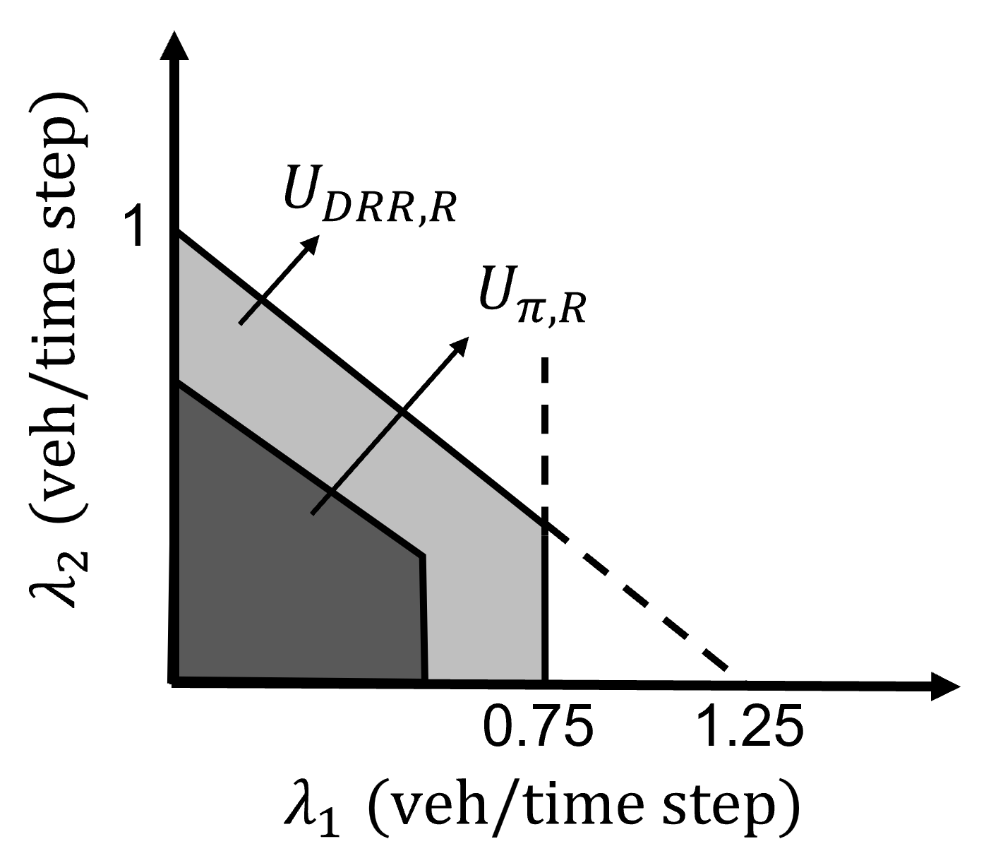
Figure 9: An illustration of the under-saturation region of some policy $\pi^{\prime}$ (dark grey area) and the DRR policy (dark + light grey areas) from Example 6.

Example 6.

(Example 3 cont’d) Consider again the $3$-ramp network with

$$R=\begin{pmatrix}0.2&0.7&0.1\\ 0&0.8&0.2\\ 0.5&0&0.5\end{pmatrix},\leavevmode\nobreak\ \lambda_{3}=0.5\leavevmode\nobreak\ [\text{veh}/\text{time step}],$$

and suppose that the merging speed at all the on-ramps is $V_{f}$, i.e, $\tau_{i}=2\tau$ for $i=1,2,3$. Let us consider the DRR policy presented in Section 4.2. By Theorem 2, the under-saturation region of this policy is given by

$$U_{\text{DRR},R}=\{(\lambda_{1},\lambda_{2}):\rho=\max_{i=1,2,3}\rho_{i}<1\}=\{(\lambda_{1},\lambda_{2}):\lambda_{1}<0.75,\leavevmode\nobreak\ 0.8\lambda_{1}+\lambda_{2}<1\},$$

which is illustrated in Figure 9. Furthermore, by Theorem 4, for any other policy $\pi^{\prime}$ we have $U_{\pi^{\prime},R}\subseteq\{(\lambda_{1},\lambda_{2}):\rho\leq 1\}$, which is a subset of $U_{\text{DRR},R}$ except, maybe, at the boundary of $U_{\text{DRR},R}$. Since the boundary of $U_{\text{DRR},R}$ has zero volume, the vector $(\lambda_{1},\lambda_{2})$ lies either inside or outside of $U_{\text{DRR},R}$ in practice. Therefore, $U_{\pi^{\prime},R}\subseteq U_{\text{DRR},R}$ for all practical purposes. Note that the previous conclusion also holds for any other choice of the routing matrix, which implies that the DRR policy maximizes the throughput for all practical purposes.

4.7 Discussion of the Straight Road Configuration

In this section, we extend our results to the straight road configuration such as the one shown in Figure 1(b). Let the number of on- and off-ramps be $m-1$; suppose that they are placed alternatively, and they are numbered in an increasing order along the direction of travel. Recall that the upstream entry point in this configuration acts as a virtual on-ramp, indicating that all the previous on-ramps are metered.

Roughly speaking, the straight road configuration is a special case of the ring road configuration with an upper triangular routing matrix. Therefore, it is natural to expect that all of our assumptions and results will apply to this setting as well. In fact, all of our assumptions remain unchanged, except for (VC3) in Section 3.1, which is slightly modified as follows:

• there exists $T_{\text{free}}$ such that for any initial condition, if no vehicle is released from the entry points $1,\ldots,j$ for some $j\in\{1,\ldots,m\}$, and all the vehicles downstream of link $j$ are at the free flow state, then all the vehicles reach the free flow state after at most $T_{\text{free}}$ seconds.

We may also assume, without loss of generality, that vehicles enter from the upstream entry point at the speed $V_{f}$ in the free flow state. This is justified since the upstream inflow is not restricted by the inflow from the on-ramps in the free flow state. With these slight modifications, the description of all the proposed policies remain unchanged for the straight road configuration. Their performance will also be the same with a slight change in the proof of Theorem 2, which is stated as needed during the proof.

Remark 10.

The results can be extended even further when we have partial control over the on-ramps, e.g., when some of the on-ramps preceding the upstream entry point in the straight road configuration are not metered. However, in that case, the throughput of the metered on-ramps may become zero for sufficiently high upstream inflow under the proposed policies. This is due to the safety considerations that prevent entry from the on-ramps, resulting in a queue forming at those on-ramps. In order to deal with this issue, an alternative approach is for the vehicles to coordinate locally, allowing the on-ramp vehicles to enter the freeway. This would shift the on-ramp queue to the freeway, which is more desirable in practice. It is important to note that vehicle coordination does not offer any additional benefits when we have full control over every on-ramp. In such cases, the need for coordination is already addressed by the proposed RM policies in place. The authors are currently exploring vehicle coordination for the partial control case in a separate paper.

5 Simulations

The following setup is common to all the simulations in this section. We consider a ring road of length $P=1860\leavevmode\nobreak\ [\text{m}]$ and $m=3$ on- and off-ramps. Let $h=1.5\leavevmode\nobreak\ [\text{sec}]$, $S_{0}=4\leavevmode\nobreak\ [\text{m}]$, $L=4.5\leavevmode\nobreak\ [\text{m}]$, and $V_{f}=15\leavevmode\nobreak\ [\text{m/sec}]$. For these parameters, we obtain $n_{c}=60$. The on-ramps are located symmetrically at $0$, $P/3$, and $2P/3$; the off-ramps are also located symmetrically $155\leavevmode\nobreak\ [\text{m}]$ upstream of each on-ramp. The initial queue size of all the on-ramps is set to zero. Vehicles arrive at the on-ramps according to i.i.d Bernoulli processes with the same rate $\lambda$; their destinations are determined by

$$R=\begin{pmatrix}0.2&0.7&0.1\\ 0&0.8&0.2\\ 0.5&0&0.5\end{pmatrix}.$$

Note that, on average, most of the vehicles want to exit from off-ramp $2$. Thus, one should expect that on-ramp $3$ finds more safe merging gaps between vehicles on the mainline than the other two on-ramps. As a result, on-ramp $3$’s queue size is expected to be less than the other two on-ramps. All the simulations were performed in MATLAB. The details of the vehicle controller is provided in Section 5.3.

5.1 Greedy Policy for Low Merging Speed

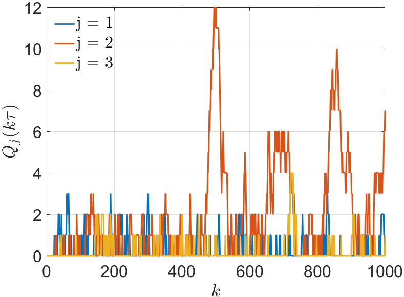
Figure 10: On-ramp queue size profiles under the FCQ policy, when all the on-ramps are long.

The mainline and acceleration lanes are assumed to be initially empty in this section and Section 5.2. The on-ramps use the Greedy policy, i.e., the FCQ policy with $T_{\text{cyc}}=1$, from Section 4.5. When the merging speed at all the on-ramps is $V_{f}$, then the throughput of the FCQ policy is $\lambda=5/9\leavevmode\nobreak\ [\text{veh}/\text{time step}]$ for the given $R$. Note that the throughput is a single point, rather than a set of points, since the arrival rates are assumed to be the same. The queue size profiles for $\lambda=0.5\leavevmode\nobreak\ [\text{veh}/\text{time step}]$, which corresponds to $\rho=0.9$ (heavy demand), is shown in Figure 10. As expected, $Q_{3}(\cdot)$ is generally less than the other two on-ramps.

We next consider the case when the merging speed at on-ramps $1$ and $3$ are $V_{f}$, i.e., $\tau_{1}=\tau_{3}=2\tau$, and is approximately $V_{f}/3=5\leavevmode\nobreak\ [\text{m/sec}]$ at on-ramp $2$ which corresponds to $\tau_{2}=3\tau$. In the heavy demand regime, i.e., $\rho=0.9$, $Q_{2}(\cdot)$ increases steadily which suggests that the freeway becomes saturated even though $\rho<1$. The throughput of the FCQ policy in this case is estimated from simulations to be $\lambda=0.44\leavevmode\nobreak\ [\text{veh}/\text{time step}]$, while the estimate given by Theorem 2 is $\lambda=0.33\leavevmode\nobreak\ [\text{veh}/\text{time step}]$. Moreover, the throughput estimate of the Renewal policy given by Theorem 1 is $\lambda=0.5\leavevmode\nobreak\ [\text{veh}/\text{time step}]$. Combining this with the simulation results, we see that the Renewal policy has a better throughput than the Greedy policy.

5.2 Effect of Cycle Length on Queue Size

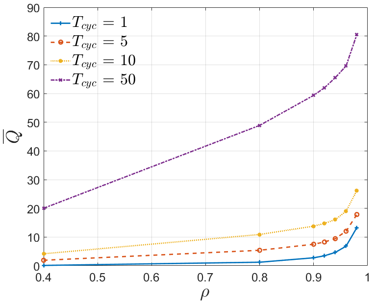
(a)

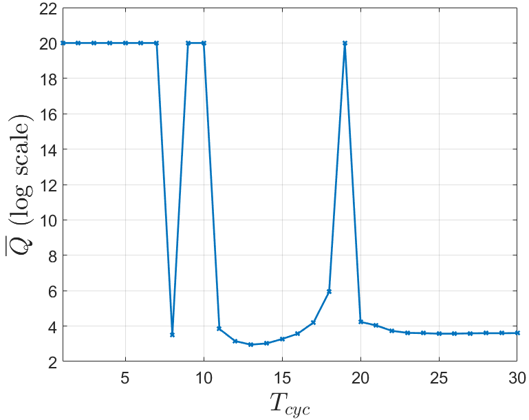
(b)

Figure 11: Effect of cycle length $T_{\text{cyc}}$ on the long-run expected queue size (a) for different $\rho$ when both on-ramps are long, (b) for a fixed $\rho$ when on-ramp $2$ is short. Both plots are under the FCQ policy. In plot (b), the logarithm of the expected queue size is set to $20$ whenever the freeway becomes saturated.

The long-run expected queue size, i.e., $\overline{Q}:=\limsup_{k\rightarrow\infty}\mathbb{E}\left[\sum_{i}Q_{i}(k\tau)\right]$, are compared under the FCQ policy for different $T_{\text{cyc}}$. The expected queue size is computed using the batch means approach, with warm-up period of $10^{5}$, i.e., the first $10^{5}$ observations are not used, and batch size of $10^{5}$. In each case, the simulations are run until the margin of error of the $95\%$ confidence intervals are $1\%$.

Figure 11(a) shows $\overline{Q}$ vs. $\rho$ for different $T_{\text{cyc}}$ when the merging speed at all the on-ramps is $V_{f}$. The plot suggests that for all $\rho$, $\overline{Q}$ increases monotonically with $T_{\text{cyc}}$. However, this does not hold true when the merging speeds are low. For example, Figure 11(b) shows $\overline{Q}$ in log scale vs. $T_{\text{cyc}}$ for $\lambda=0.455\leavevmode\nobreak\ [\text{veh}/\text{time step}]$, which corresponds to $\rho\approx 0.82$, when the merging speed at on-ramps $1$ and $3$ is $V_{f}$, and is $V_{f}/3$ at on-ramp $2$. As the plot shows, depending on the choice of $T_{\text{cyc}}$, the freeway may become saturated which causes the expected queue size to grow over time, i.e., $\overline{Q}=\infty$ (in the plot, $\log\overline{Q}$ is set to $20$ whenever this occurs). Moreover, one can see from Figure 11(b) that the dependence of $\overline{Q}$ on $T_{\text{cyc}}$ is not monotonic in the low merging speed case. In fact, the optimal choice of $T_{\text{cyc}}$ in this case is $13$.

5.3 Relaxing the V2X Requirements

In this scenario, we evaluate the performance of the Greedy policy for $\rho=0.9$ (heavy demand) when the merging speed at all the on-ramps is $V_{f}$, and the mainline is initially not empty. The safety mode only consists of the following submode: in a non-merging scenario, the ego vehicle follows the leading vehicle by keeping a safe time headway as in, e.g., Pooladsanj et al., (2022). For this control law, platoons of vehicles are stable and string stable (Pooladsanj et al., (2022)). In a merging scenario, it applies the above control law with respect to both its leading and virtual leading vehicles. The most restrictive acceleration is used by the ego vehicle.

The initial number of vehicles on the mainline, their location, and their speed are chosen at random such that the safety distance is not violated. The initial acceleration of all the vehicles is set to zero. We conducted $10$ rounds of simulation with different random seed for each round. It is observed in all scenarios that vehicles reach the free flow state after a finite time using the Greedy policy. We conjecture that this observation holds for any initial condition if platoons of vehicles are stable and string stable. The intuition behind this conjecture is as follows: under the Greedy policy, vehicles are released only if there is sufficient gap between vehicles on the mainline, and successive releases are at least $\tau$ seconds apart. In between releases, vehicles on the mainline try to reach the free flow state because of platoon stability. Once a vehicle is released, it may create disturbance, e.g., in the acceleration of the upstream vehicles. However, string stability ensures that such disturbance is attenuated. Therefore, it is natural to expect that the vehicles reach the free flow state after a finite time. Thereafter, by Theorem 2, the Greedy policy keeps the freeway under-saturated if $(\tau_{i}/\tau-1)\rho_{i}<1$ for all $i\in[m]$.

5.4 Comparing the Total Travel Time

We evaluate the total travel time under the Renewal, DRR, DisDRR, DSG, and Greedy policies, which use accurate traffic measurements obtained by V2I communication. We compare these results against the ALINEA RM policy (Papageorgiou et al., (1991)), which relies on local traffic measurements obtained by roadside sensors. The purpose of this comparison is to illustrate how much V2I communication can improve performance when comparing with a well-known RM policy which relies only on roadside sensors. The ALINEA policy controls the outflow of an on-ramp according to the following equation:

$$r(k)=r(k-1)+K_{r}(\hat{o}-o(k)).$$

Here, $r(\cdot)$ is the on-ramp outflow, $K_{r}$ is a positive design constant, $o(\cdot)$ is the occupancy of the mainline downstream of the on-ramp, and $\hat{o}$ is the desired occupancy. For the ALINEA policy, we use time steps of size $60\leavevmode\nobreak\ [\text{sec}]$, $K_{r}=70\leavevmode\nobreak\ [\text{veh/h}]$ (Papageorgiou et al., (1991)), and $\hat{o}=13\leavevmode\nobreak\ \%$ corresponding to the mainline flow capacity. We also add the following vehicle following safety filter on top of ALINEA: the ego vehicle is released only if it is predicted to be at a safe distance with respect to its virtual leading and following vehicles at the moment of merging. We use the name Safe-ALINEA to refer to this policy. For the DRR and DisDRR policies, we use the following parameters: $T_{\text{cyc}}=13$, $T_{\text{per}}=2\tau$, $\gamma_{1}=50$, $\gamma_{2}=10$, $\theta_{i}^{\circ}=0.1$, $\beta=1.01$, and $T_{\text{max}}=100\leavevmode\nobreak\ [\text{sec}]$. Informally, $\gamma_{1}$ is set to a high value so that the release times $g_{i}(\cdot)$ increase if the traffic condition, i.e., the value of $X_{f}$, does not improve significantly in between the update periods; $\gamma_{2}$ and $\theta_{i}^{\circ}$ are set to low values so that the jump sizes in $g_{i}(\cdot)$ are small; $T_{\text{max}}$ is set to a high value so that on-ramps update their release time in a completely decentralized way. For the DSG policy, we set $T_{\text{cyc}}=13$ and use the additional space gap $\kappa_{1}X_{f_{1}}+\kappa_{2}\sum_{e\in[n]}|y_{e}-(hv_{e}+S_{0})|I_{e}$ on top of (M3)-(M4), where $\kappa_{1}=\kappa_{2}=0.01$ are chosen so that the additional space gap is relatively small ($\approx 8\leavevmode\nobreak\ [\text{m}]$ for the initial condition described next).

We let the merging speed at on-ramps $1$ and $3$ be $V_{f}$, and $V_{f}/3$ at on-ramp $2$. We let $\lambda=0.455\leavevmode\nobreak\ [\text{veh}/\text{time step}]$, and consider a congested initial condition where the initial number of vehicles on the mainline is $100>n_{c}$; each vehicle is at the constant speed of $6.7\leavevmode\nobreak\ [\text{m/sec}]$, and is at the distance $h\times 6.7+S_{0}\approx 14.1\leavevmode\nobreak\ [\text{m}]$ from its leading vehicle.

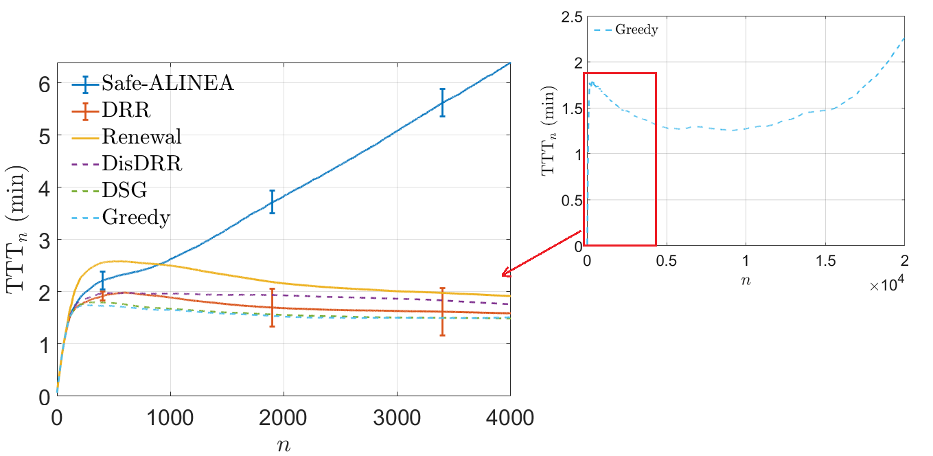
Figure 12: The average value of the total travel time of the first $n$ vehicles that complete their trips ($\text{TTT}_{n}$) for the fixed demand $\rho=0.82$. The vertical lines in the Safe-ALINEA and DRR policies represent the standard deviation. The standard deviation of the Renewal, DisDRR, DSG, and Greedy policies were similar to the DRR policy and are omitted for clarity. The smaller figure on the top right shows $\text{TTT}_{n}$ under the Greedy policy over a longer time horizon, with trajectories of the DRR, Renewal, DisDRR, and DSG policies removed due to their non-increasing behavior.

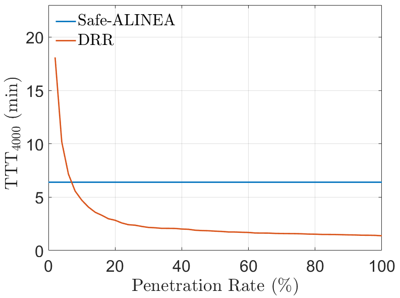
Figure 13: The average travel time, i.e., $\text{TTT}_{4000}$, under the Safe-ALINEA and DRR policies at different penetration rates of connected vehicles for the fixed demand $\rho=0.82$.

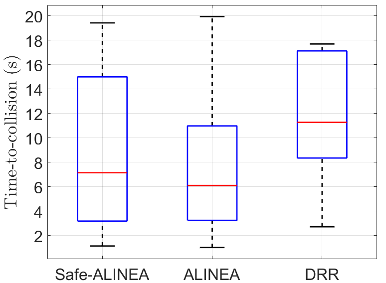
Figure 14: Time-to-collision near on-ramp $2$ under the Safe-ALINEA, ALINEA, and DRR policies. On each box, the red line indicates the median, and the bottom and top edges of the box indicate the $25$-th and $75$-th percentiles, respectively. The whiskers extend to the most extreme data points not considered outliers.

We compute the average value of Total Travel Time (TTT_n), which is computed by averaging the total travel time of the first $n$ vehicles that complete their trips. The total travel time of a vehicle equals its waiting time in an on-ramp queue plus the time it spends on the freeway to reach its destination. In order to show consistency, we have conducted $10$ rounds of simulations with different random seed for each round and averaged the results over the $10$ simulation rounds.

For the setup described above, the Safe-ALINEA and Greedy policies fail to keep the freeway under-saturated, whereas the other policies keep it under-saturated. From Figure 12 and Table 3, we can see that the DRR policy provides significant improvement in the average travel time, i.e., TTT₄₀₀₀, compared to the Safe-ALINEA policy (approximately $75\%$). The Renewal, DisDRR, and DSG policies show similar improvements. Figure 12 also shows that while the Greedy policy initially improves TTT_n, this improvement disappears over time since the freeway becomes saturated for $T_{\text{cyc}}=1$ as shown in Section 5.2. On the other hand, the choice of $T_{\text{cyc}}=13$ in the DRR, DisDRR, and DSG policies will show steady improvement.

Next, we evaluate the performance of the DRR policy in scenarios where some vehicles lack V2I communication capabilities. In such cases, we assume that the DRR policy relies only on the measurements obtained from the connected vehicles and ignores the non-connected vehicles. Figure 13 shows the average travel time, i.e., TTT₄₀₀₀, under the safe-ALINEA and DRR policies at different penetration rates of connected vehicles. As can be seen, the average travel time increases as the penetration rate decreases. However, even at low penetration rates, the DRR policy provides improvement over the Safe-ALINEA policy.

Finally, at a 100$\%$ penetration rate of connected vehicles, Table 3 provides the time average queue size, i.e., $\overline{Q}(K\tau)=\frac{1}{mK}\sum_{i,j}Q_{i}(j\tau)$, where $Q_{i}$ is averaged over the $10$ simulation rounds and $K\tau$ is the simulation time. It can be seen that the Safe-ALINEA policy has the largest queue size compared to the other policies. This is mainly because of the safety filter added on top of the ALINEA policy. Without the safety filter, ALINEA releases vehicles more frequently, which results in shorter on-ramp queues on average but degrades safety. To see the latter, we use the Time-To-Collision (TTC) metric to compare safety under the Safe-ALINEA, ALINEA, and DRR policies. The TTC is defined as the time left until a collision occurs between two vehicles if both vehicles continue on the same course and maintain the same speed (Vogel, (2003)). Generally, scenarios with a TTC of at least $6$ seconds is considered to be safe (Vogel, (2003)). Figure 14 compares the TTC statistics near on-ramp $2$, where we have discarded the TTC values higher than $20$ seconds. As expected, the ALINEA policy leads to more unsafe situations compared to the other two policies. Furthermore, one can see that the safety filter in the Safe-ALINEA policy cannot remove the low TTC values in the ALINEA policy. This is due to the fact that the traffic measurements in the Safe-ALINEA policy are still local and not as accurate as the DRR policy.

In conclusion, with proper choice of design parameters, the proposed policies reduce the risk of collision at the merging bottlenecks without compromising travel time.

Table 3: Performance of the policies.

Ramp Metering Policy	Renewal	DRR	DisDRR	DSG	Greedy	Safe-ALINEA
Average travel time $[\text{min}]$	1.9	1.6	1.8	1.5	1.5	6.4
Average queue size	156	8	15	9	14	677

5.5 The Capacity Drop Phenomenon

It is known that the maximum achievable traffic flow downstream of a merging bottleneck may decrease when queues are formed, i.e., the capacity drop phenomenon (Hall and Agyemang-Duah, (1991)). In this section, we compare the capacity drop downstream of on-ramp $2$ under the DRR and Safe-ALINEA policies. For both policies, we use the parameters of Section 5.4. Similar to Section 5.4, we let the merging speed at on-ramps $1$ and $3$ be $V_{f}$, and $V_{f}/3$ at on-ramp $2$, and we let $\lambda=0.455\leavevmode\nobreak\ [\text{veh}/\text{time step}]$. We consider an initial condition where the density is at its critical value (at which the mainline flow is maximized), i.e., the initial number of vehicles on the mainline is $60=n_{c}$; each vehicle is at the constant free flow speed, and is at the safe distance $hV_{f}+S_{0}=26.5\leavevmode\nobreak\ [\text{m}]$ from its leading vehicle.

Figure 15 shows the simulation results, where we have let the simulation run idly in the first $5$ minutes without any vehicle entering or exiting the network. As can be seen, both policies lead to a capacity drop downstream of on-ramp $2$, but the capacity drop under the Safe-ALINEA policy is on average $15\%$ worse than the DRR policy. This is not surprising as the DRR policy uses more accurate traffic measurements to maintain the free flow state. We should note, however, that the capacity drop in both cases occur mainly because of the vehicle following safety considerations and the low merging speed at on-ramp $2$, rather than the formation of queues near the merging point, which is the usual reason for capacity drop. In particular, because of the low merging speed at on-ramp $2$, the minimum distance between vehicles on the mainline that is required by both policies is greater than $hV_{f}+S_{0}$ at the free flow state. This would reduce the mainline flow when the mainline vehicles are at a distance greater than $hV_{f}+S_{0}$ but less than the threshold required by both policies. It is worth discussing the case where the merging speed at an on-ramp is $V_{f}$. In this case, the capacity drop under the DRR policy with $T_{\text{cyc}}=1$ will disappear after the vehicles reach the free flow state. This is because, at the free flow state, the minimum distance between vehicles on the mainline that is required by the DRR policy is $hV_{f}+S_{0}$. Since $T_{\text{cyc}}=1$, every gap that is at least $hV_{f}+S_{0}$ will be used greedily by the on-ramp, thus maintaining the maximum flow.

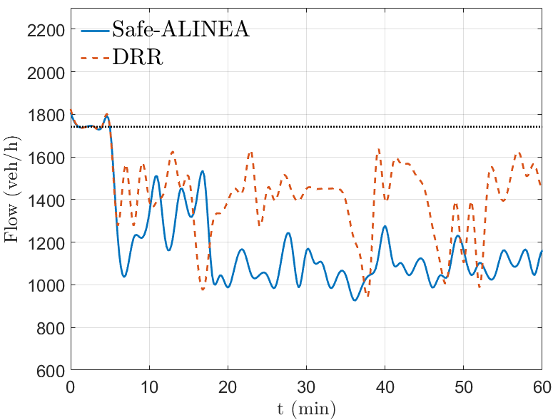
Figure 15: The traffic flow downstream of on-ramp $2$ under the Safe-ALINEA and DRR policies. The dotted black line indicates the mainline capacity.

6 Conclusion and Future Work

We provided a microscopic-level RM framework subject to vehicle following safety constraints. This allows to explicitly take into account vehicle following safety and V2X communication scenarios in the design of RM, and study their impact on the freeway performance. We specifically provided RM policies that operate under vehicle following safety constraints, and analyzed performance in terms of their throughput. The proposed policies work in synchronous cycles during which an on-ramp does not release more vehicles than the number of vehicles waiting in its queue at the start of the cycle. The cycle length was variable in the Renewal policy, which could increase the total travel time. To prevent this issue, we used a fixed cycle length in the other policies. A fixed cycle length, however, can reduce the throughput when the merging speeds are less than the free flow speed. When the merging speeds are all equal to the free flow speed, all the proposed policies maximize the throughput. We compared the performance of the proposed policies with a well-known macroscopic RM policy that relies on local traffic measurements obtained from roadside sensors. We observed considerable improvements in the total travel time, capacity drop, and time-to-collision performance metrics.

There are several avenues for generalizing the setup and methodologies initiated in this paper. Of immediate interest would be to consider a general network structure, and to derive sharper inner-estimates on the under-saturation region for the low merging speed case. We are also interested in expanding performance analysis to include travel time, possibly by leveraging waiting time analysis from queuing theory. Finally, we plan to conduct simulations using a high-fidelity traffic simulator to evaluate the performance of the proposed policies in mixed traffic scenarios, where some vehicles are manually driven.

Appendix A Network Specifications

A.1 Dynamics in the Speed Tracking Mode

Suppose that the ego vehicle is in the speed tracking mode for all $t\geq 0$, $v_{e}(0)=v_{0}\in[0,V_{f}]$, and $a_{e}(0)=a_{0}\in[a_{\min},a_{\max}]$, where $a_{e}$ is the acceleration and $a_{\max}$ is the maximum possible acceleration. Then, for a third-order vehicle dynamics, we have

$$v_{e}(t) =v_{0}+\int_{0}^{t}a_{e}(\xi)d\xi$$

$$a_{e}(t) =\begin{cases*}J_{\max}t+a_{0}&\mbox{if } $0\leq t<t_{1}$\\ a_{\max}&\mbox{if } $t_{1}\leq t<t_{1}+t_{2}$\\ a_{\max}-J_{\max}t&\mbox{if } $t_{1}+t_{2}\leq t<t_{1}+t_{2}+t_{3}$\\ 0&\mbox{if } $t\geq t_{1}+t_{2}+t_{3}$\end{cases*},$$

where $J_{\max}$ is the maximum possible jerk, $t_{1}$ is the time at which the ego vehicle reaches the maximum acceleration, $t_{2}$ is the additional time required to reach a desired speed before it decelerates, and $t_{3}$ is the time required to reach the zero acceleration in order to avoid exceeding the speed limit $V_{f}$. Hence, $v_{e}(t_{1}+t_{2}+t_{3})=V_{f}$, and $a_{e}(t_{1}+t_{2}+t_{3})=0$. The dynamics for the $v_{0}>V_{f}$ case is similar.

A.2 Communication Cost of a Ramp Metering Policy

The calculation of the communication cost for a policy is inspired by the robotics literature (Bullo et al., (2009, Remark 3.27)). We let $C_{ij}(k)=1$ if vehicle $i$ communicates with on-ramp $j$ at time $k\tau$, and $C_{ij}(k)=0$ otherwise. Then, the total number of transmissions at time $k\tau$ is $C(k)=\sum_{i\in[n],j\in[m]}C_{ij}(k)$, where $n$ is the total number of vehicles in the network. The communication cost of the policy, measured in number of transmissions per $\tau$ seconds, is obtained as follows:

$$C=\limsup_{K\rightarrow\infty}\frac{1}{K}\sum_{k=0}^{K-1}C(k).$$

Appendix B Performance Analysis Tool

Recall the initial condition from Section 3.3, where the vehicles are in the free flow state and the location of each vehicle coincides with a slot for all times in the future. For this initial condition and under the proposed RM policies, we can cast the network as a discrete-time Markov chain. With a slight abuse of notation, we let $t=0,1,\ldots$ with time steps of duration $\tau$ whenever we are talking about the underlying Markov chain. Let $M_{i}^{q}(t)$ be the vector of destination off-ramps of the vehicles that are waiting at on-ramp $i$ at $t$, arranged in the order of their arrival. Furthermore, let $M^{s}(t)=[M_{\ell}^{s}(t)]$ be the vector of the destination off-ramps of the occupants of the $n_{c}+n_{a}$ slots: $M_{\ell}^{s}(t)=j$ if the vehicle occupying slot $\ell$ at time $t$ wants to exit from off-ramp $j$, and $M_{\ell}^{s}(t)=0$ if slot $\ell$ is empty at time $t$. Consider the following discrete-time Markov chain with the state

$$Y(t):=(M_{1}^{q}(t),\ldots,M_{m}^{q}(t),M^{s}(t)).$$

The transition probabilities of this chain are determined by the RM policy being analyzed, but will not be specified explicitly for brevity. For all the RM policies considered in this paper, the state $Y(t)=(0,0)$ is reachable from all other states, and $\mathbb{P}\left(Y(t+1)=(0,0)\leavevmode\nobreak\ |\leavevmode\nobreak\ Y(t)=(0,0)\right)>0$. Hence, the chain $Y$ is irreducible and aperiodic. In the the proofs of Theorem 1 and 2, we construct new Markov chains (that are also irreducible and aperiodic) by “thinning" the chain $Y$.

The following is an adaptation of a well-known result, e.g., see Meyn and Tweedie, (2012, Theorem 14.0.1), for the setting of our paper.

Theorem 5.

(Foster-Lyapunov drift criterion) Let $\{Z(t)\}_{t=1}^{\infty}$ be an irreducible and aperiodic discrete time Markov chain evolving on a countable state space $\mathcal{Z}$. Suppose that there exist $V:\mathcal{Z}\rightarrow[0,\infty)$, $f:\mathcal{Z}\rightarrow[1,\infty)$, a finite constant $b$, and a finite set $B\in\mathcal{Z}$ such that, for all $z\in\mathcal{Z}$,

$$\mathbb{E}\left[V(Z(t+1))-V(Z(t))|\>Z(t)=z\right]\leq-f(z)+b\mathbbm{1}_{B}(z),$$ (3)

where $\mathbbm{1}_{B}(z)$ is the indicator function of the set $B$. Then, $\lim_{t\rightarrow\infty}\mathbb{E}\left[f(Z(t))\right]$ exists and is finite.

Remark 11.

If the conditions of Theorem 5 hold true, then $V$ is referred to as a Lyapunov function. Additionally, if $f(Z(t))=\|Q(t)\|_{\infty}$, where $\|Q(t)\|_{\infty}$ denotes the sup norm of the vector of queue sizes $Q(t)$, then $\lim_{t\rightarrow\infty}\mathbb{E}\left[\|Q(t)\|_{\infty}\right]<\infty$, and hence $\limsup_{t\rightarrow\infty}\mathbb{E}\left[Q_{i}(t)\right]<\infty$ for all $i\in[m]$.

We end this section by introducing a notation which will be used in the proofs of Theorem 1 and 2 to construct Lyapunov functions and/or prove certain results about them. Given on-ramp $i\in[m]$, we let $N_{i}(t)$ be the degree of on-ramp $i$ at time $t$, which represents the number of vehicles in the network at time $t$ that need to cross the merging point of on-ramp $i$ in order to reach their destination.

Appendix C Proofs of the Main Results

C.1 Proof of Theorem 1

For the sake of readability, we present proofs of intermediate claims at the end. Under the Renewal policy, the first cycle starts when the vehicles reach the free flow state, which is after at most $T_{\text{free}}$ seconds by (VC3). The free flow state and (M4) imply that any vehicle that is released thereafter remains in the speed tracking mode in the future, which implies that the location of the released vehicles coincide with a slot for all times in the future. Without loss of generality, let the start of the first cycle $t_{1}$ be at time $0$, and let the location of each vehicle coincides with a slot at time $0$. We can adopt the Markov chain setting from Appendix B with $\{Y(t_{k})\}_{k\geq 1}$ as the Markov chain, where $t_{k}$ is the start of the $k$-th cycle. Consider the function $V:\mathcal{Y}\rightarrow[0,\infty)$

$$V(Y(t_{k}))=T_{\text{cyc}}^{2}(k),$$

where $\mathcal{Y}$ is the range of values of $Y$, and $T_{\text{cyc}}(k)=t_{k+1}-t_{k}$ is the length of the $k$-th cycle. We let $V(Y(t_{k}))\equiv V(t_{k})$ for brevity. It is shown at the end of the proof that

$$T_{\text{cyc}}(k+1)\leq\tilde{A}(T_{\text{cyc}}(k))+n_{c}+n_{a},$$ (4)

where $\tilde{A}(T_{\text{cyc}}(k))$ depends on the number of arrivals in the interval $[t_{k}+1,t_{k+1}]$ and satisfies the following:

$$\lim_{t\rightarrow\infty}\mathbb{E}\left[\left(\frac{\tilde{A}(T_{\text{cyc}}(k))}{T_{\text{cyc}}(k)}\right)^{2}\middle|\leavevmode\nobreak\ T_{\text{cyc}}(k)=t\right]=\left(\max_{i\in[m]}(\frac{\tau_{i}}{\tau}-1)\rho_{i}-(\frac{\tau_{i}}{\tau}-2)\lambda_{i}\right)^{2}.$$ (5)

By the assumption of the Theorem, $(\tau_{i}/\tau-1)\rho_{i}-(\tau_{i}/\tau-2)\lambda_{i}<1$ for all $i\in[m]$. Combining this with (4) and (5), it follows that

$$\limsup_{t\rightarrow\infty}\mathbb{E}\left[\left(\frac{T_{\text{cyc}}(k+1)}{T_{\text{cyc}}(k)}\right)^{2}\middle|\leavevmode\nobreak\ T_{\text{cyc}}(k)=t\right] \leq\limsup_{t\rightarrow\infty}\mathbb{E}\left[\left(\frac{\tilde{A}(T_{\text{cyc}}(k))}{T_{\text{cyc}}(k)}\right)^{2}\middle|\leavevmode\nobreak\ T_{\text{cyc}}(k)=t\right]$$

$$=\left(\max_{i\in[m]}(\frac{\tau_{i}}{\tau}-1)\rho_{i}-(\frac{\tau_{i}}{\tau}-2)\lambda_{i}\right)^{2}<1.$$

Therefore, there exists $\delta\in(0,1)$ and $T>0$ such that for all $t>T$ we have

$$\mathbb{E}\left[\left(\frac{T_{\text{cyc}}(k+1)}{T_{\text{cyc}}(k)}\right)^{2}\middle|\leavevmode\nobreak\ T_{\text{cyc}}(k)=t\right]<1-\delta,$$

which in turn implies that

$$\mathbb{E}\left[T_{\text{cyc}}^{2}(k+1)-T_{\text{cyc}}^{2}(k)\middle|\leavevmode\nobreak\ T_{\text{cyc}}(k)>T\right]<-\delta T_{\text{cyc}}^{2}(k).$$

Since $Q_{i}(t_{k})\leq T_{\text{cyc}}(k)\leq T_{\text{cyc}}^{2}(k)$ for all $i\in[m]$, it follows that $\mathbb{E}\left[T_{\text{cyc}}^{2}(k+1)-T_{\text{cyc}}^{2}(k)\middle|\leavevmode\nobreak\ T_{\text{cyc}}(k)>T\right]<-\delta\|Q(t_{k})\|_{\infty}$, where $\|Q\|_{\infty}=\max_{i}Q_{i}$ as defined in Appendix B.

If $T_{\text{cyc}}(k)\leq T$, then $\tilde{A}(T_{\text{cyc}}(k))$ is shown in (8) to satisfy $\tilde{A}(T_{\text{cyc}}(k))\leq mT\max_{is\in[m]}(\tau_{i}/\tau-1)$. Combining this with (4) gives $T_{\text{cyc}}(k+1)\leq mT\max_{i\in[m]}(\tau_{i}/\tau-1)+n_{c}+n_{a}$. Therefore, $\mathbb{E}\left[T_{\text{cyc}}^{2}(k+1)\middle|\leavevmode\nobreak\ T_{\text{cyc}}(k)\leq T\right]\leq\left(mT\max_{i\in[m]}(\tau_{i}/\tau-1)+n_{c}+n_{a}\right)^{2}+T_{\text{cyc}}^{2}(k)-\delta\|Q(t_{k})\|_{\infty}$, where we have used $\delta\|Q(t_{k})\|_{\infty}\leq\|Q(t_{k})\|_{\infty}\leq T_{\text{cyc}}^{2}(k)$.

Combining all the previous steps gives

$$\mathbb{E}\left[V(t_{k+1})-V(t_{k})\middle|\leavevmode\nobreak\ Y(t_{k})\right]\leq-\delta\|Q(t_{k})\|_{\infty}+\left(mT\max_{i\in[m]}(\frac{\tau_{i}}{\tau}-1)+n_{c}+n_{a}\right)^{2}\mathbbm{1}_{B},$$

where $B=\{Y(t_{k}):V(t_{k})\leq T^{2}\}$ (a finite set). The result then follows from Theorem 5.

Proof of (4)

Consider the $(k+1)$-th cycle. Let $s_{i}\in[t_{k+1},t_{k+2})$ be the time at which the queue at on-ramp $i\in[m]$ becomes empty of the $(k+1)$-th cycle quota. We claim that

$$s_{i}-t_{k+1}\leq(\frac{\tau_{i}}{\tau}-1)N_{i}(t_{k+1})-(\frac{\tau_{i}}{\tau}-2)Q_{i}(t_{k+1})+n_{c}+n_{a},$$

where $N_{i}$ is defined in Appendix B. Suppose not, i.e.,

$$s_{i}-t_{k+1}-\left((\frac{\tau_{i}}{\tau}-1)(N_{i}(t_{k+1})-Q_{i}(t_{k+1}))+n_{c}+n_{a}\right)>Q_{i}(t_{k+1}).$$ (6)

We will use (6) to reach a contradiction. If at least one upstream vehicle crosses the merging point of on-ramp $i$ in $\tau_{i}/\tau-1$ time steps, then the last acceleration lane slot of on-ramp $i$ that is not on the mainline must be empty because of the vehicle following safety consideration (M4). Since the total number of vehicles from other on-ramps that need to cross the merging point of on-ramp $i$ is $N_{i}(t_{k+1})-Q_{i}(t_{k+1})$, and the number of vehicles from cycle $k$ that are still on the freeway at the start of the $(k+1)$-th cycle is at most $n_{c}+n_{a}$, the aforementioned acceleration lane slot can be empty of the $(k+1)$-th cycle quota for at most $(\tau_{i}/\tau-1)(N_{i}(t_{k+1})-Q_{i}(t_{k+1}))+n_{c}+n_{a}$ time steps. Therefore, it must be occupied for at least $s_{i}-t_{k+1}-\left((\tau_{i}/\tau-1)(N_{i}(t_{k+1})-Q_{i}(t_{k+1}))+n_{c}+n_{a}\right)$ time steps, which by (6) is greater than $Q_{i}(t_{k+1})$. This, however, contradicts the feature of the Renewal policy under which the number of vehicles released by an on-ramp during a cycle does not exceed the queue size at the start of the cycle.

Since $T_{\text{cyc}}(k+1)\leq\max_{i\in[m]}s_{i}-t_{k+1}+n_{c}+n_{a}$, it follows that

$$T_{\text{cyc}}(k+1)\leq\max_{i\in[m]}\left\{(\frac{\tau_{i}}{\tau}-1)N_{i}(t_{k+1})-(\frac{\tau_{i}}{\tau}-2)Q_{i}(t_{k+1})\right\}+n_{c}+n_{a}.$$ (7)

Let $A_{i}(s)$ be the number of arrivals to on-ramp $i$ at time $s$, and $A_{\ell,i}(s)$ be the number of arrivals to all the on-ramps at time $s$ that need to cross link $i$. We let $\bar{A}_{i}(t_{k+1}-t_{k})$ denote the cumulative number of arrivals to on-ramp $i$ during the interval $[t_{k}+1,t_{k+1}]$, i.e.,

$$\bar{A}_{i}(t_{k+1}-t_{k})=\sum_{s=t_{k}+1}^{t_{k+1}}A_{i}(s).$$

We define $\bar{A}_{\ell,i}(t_{k+1}-t_{k})$ similarly. Note that $Q_{i}(t_{k+1})$ is precisely the cumulative number of arrivals to on-ramp $i$ in $[t_{k}+1,t_{k+1}]$, i.e., $Q_{i}(t_{k+1})=\bar{A}_{i}(t_{k+1}-t_{k})$. Similarly, $N_{i}(t_{k+1})=\bar{A}_{\ell,i}(t_{k+1}-t_{k})$. This and (7) imply (4) with

$$\tilde{A}(T_{\text{cyc}}(k))=\max_{i\in[m]}\left\{(\frac{\tau_{i}}{\tau}-1)\bar{A}_{\ell,i}(t_{k+1}-t_{k})-(\frac{\tau_{i}}{\tau}-2)\bar{A}_{i}(t_{k+1}-t_{k})\right\}.$$

Note that because the number of arrivals to all the on-ramps is at most $m$ at each time step, we have

$$\tilde{A}(T_{\text{cyc}}(k))\leq mT_{\text{cyc}}(k)\max_{i\in[m]}(\tau_{i}/\tau-1).$$ (8)

Proof of (5)

Consider the sequences $\{A_{i}(s)\}_{s=t_{k}+1}^{\infty}$ and $\{A_{\ell,i}(s)\}_{s=t_{k}+1}^{\infty}$. Each sequence is i.i.d and $\mathbb{E}\left[A_{i}(s)\right]=\lambda_{i}$, $\mathbb{E}\left[A_{\ell,i}(s)\right]=\rho_{i}$. By the strong law of large numbers, with probability one,

$$\lim_{T_{\text{cyc}}(k)\rightarrow\infty}\frac{(\tau_{i}/\tau-1)\bar{A}_{\ell,i}(t_{k+1}-t_{k})-(\tau_{i}/\tau-2)\bar{A}_{i}(t_{k+1}-t_{k})}{T_{\text{cyc}}(k)}=(\frac{\tau_{i}}{\tau}-1)\rho_{i}-(\frac{\tau_{i}}{\tau}-2)\lambda_{i}.$$

If the sequence $\left\{\left(\frac{\tilde{A}(T_{\text{cyc}}(k))}{T_{\text{cyc}}(k)}\right)^{2}\right\}_{T_{\text{cyc}}(k)=1}^{\infty}$ is upper bounded by an integrable function, then similar to the proof of Lemma 1 in Georgiadis et al., (1995) it follows that

$$\lim_{T_{\text{cyc}}(k)\rightarrow\infty}\mathbb{E}\left[\left(\frac{\tilde{A}(T_{\text{cyc}}(k))}{T_{\text{cyc}}(k)}\right)^{2}\right]=\left(\max_{i\in[m]}(\frac{\tau_{i}}{\tau}-1)\rho_{i}-(\frac{\tau_{i}}{\tau}-2)\lambda_{i}\right)^{2},$$

which in turn gives (5). The upper bound follows from the following fact: the number of arrivals to all the on-ramps is at most $m$ at each time step. Thus,

$$\frac{\tilde{A}(T_{\text{cyc}}(k))}{T_{\text{cyc}}(k)} =\frac{1}{T_{\text{cyc}}(k)}\max_{i\in[m]}\left((\frac{\tau_{i}}{\tau}-1)\bar{A}_{\ell,i}(t_{k+1}-t_{k})-(\frac{\tau_{i}}{\tau}-2)\bar{A}_{i}(t_{k+1}-t_{k})\right)$$

$$\leq\frac{1}{T_{\text{cyc}}(k)}\max_{i\in[m]}(\frac{\tau_{i}}{\tau}-1)\bar{A}_{\ell,i}(t_{k+1}-t_{k})\leq\max_{i\in[m]}(\frac{\tau_{i}}{\tau}-1)m,$$

as desired.

C.2 Proof of Theorem 2

We first show that for any initial condition, there exists $k_{0}\in\mathbb{N}$ such that $X_{f}(kT_{\text{per}})=0$ for all $k\geq k_{0}$. That is, $X_{f_{1}}(kT_{\text{per}})=0$ for all $k\geq k_{0}$ and $X_{f_{2}}(t)=0$ for all $t\geq k_{0}T_{\text{per}}$. The equality $X_{f_{2}}(t)=0$ for all $t\geq k_{0}T_{\text{per}}$ implies that each vehicle remains at a safe distance with respect to its leading vehicle, and predicts to be at a safe distance with respect to its virtual leading vehicle in merging areas. This and (VC2) imply that if a vehicle is in the speed tracking at time $k_{0}T_{\text{per}}$, it remains in this mode in the future. Furthermore, if a vehicle is in the safety mode at time $k_{0}T_{\text{per}}$, $X_{f_{1}}(k_{0}T_{\text{per}})=0$ implies that it moves at the constant speed $V_{f}$. Together with (VC1) and $X_{f_{2}}(t)=0$ for all $t\geq k_{0}T_{\text{per}}$, it follows that the vehicle maintains its speed in the future. All this would imply that the vehicles reach and remain in the free flow state at time $k_{0}T_{\text{per}}$. Hence, after a finite time after $k_{0}T_{\text{per}}$, $g(\cdot)=0$, the location of all the vehicles coincide with a slot, and we can use the Markov chain setting from Appendix B.

Recall from Remark 6 that $v_{e}$ and $\delta_{e}+\hat{\delta}_{e}$ are bounded. Let $P_{a}$ be the total length of all the acceleration lane. Since successive releases from an on-ramp are at least $\tau$ seconds apart, the number of vehicles that communicate $\delta_{e}+\hat{\delta}_{e}$ in $[t-T_{\text{per}},t]$ is at most $mT_{\text{per}}/\tau+(P+P_{a})/L$. One can then easily show that $X_{f}(t)$ is upper bounded by

$$\bar{X}:=\frac{mT_{\text{per}}}{\tau}+2\frac{P+P_{a}}{L}.$$

To show $X_{f}(\cdot)=0$ after a finite time, we use a proof by contradiction. Suppose that $X_{f}(kT_{\text{per}})\neq 0$ for infinitely many $k\in\mathbb{N}$. Since $X_{f}(kT_{\text{per}})\leq\bar{X}$ for all $k\in\mathbb{N}$, there exists an infinite sequence $\{k_{n}\}_{n\geq 1}$ such that $X_{f}(k_{n}T_{\text{per}})>X_{f}((k_{n}-1)T_{\text{per}})-\gamma_{1}$ for all $n\geq 1$. This implies that $\theta(k_{n}T_{\text{per}})=\beta\theta((k_{n}-1)T_{\text{per}})$ for all $n\geq 1$. Since $\theta(\cdot)$ is non-decreasing and $\beta>1$, it follows that $\lim_{t\rightarrow\infty}\theta(t)=\infty$, which in turn implies that $\limsup_{t\rightarrow\infty}g(t)=\infty$. Let $t_{f}$ be such that $g(t_{f})>mT_{\text{free}}(1+\gamma_{2}/T_{\text{per}})$. Note that for all $t\in[t_{f},t_{f}+mT_{\text{free}}]$, $g(t)>mT_{\text{free}}$. Thus, each on-ramp releases at most one vehicle during the interval $[t_{f},t_{f}+mT_{\text{free}}]$. Hence, there exists a time interval of length at least $T_{\text{free}}$ seconds in $[t_{f},t_{f}+mT_{\text{free}}]$ during which no on-ramp releases a vehicle. Condition (VC3) then implies that the vehicles will reach the free flow state at the end of such a time interval. This and (M4) imply that any vehicle that is released thereafter will remain in the speed tracking mode. Thus, $X_{f}(kT_{\text{per}})=0$ for all $k\geq k_{0}$ for some $k_{0}\in\mathbb{N}$; a contradiction to the assumption that $X_{f}(kT_{\text{per}})\neq 0$ for infinitely many $k$.

Without loss of generality, we let $g(0)=0$, and we assume that the vehicles are initially in the free flow state, and their location coincide with a slot as in Appendix B. For the sake of readability, we present proofs of intermediate claims at the end. We adopt the Markov chain setting from Appendix B with $\{Y(t\triangle)\}_{t\geq 0}$ as the Markov chain, where $\triangle$ is an exact multiple of the cycle length $T_{\text{cyc}}$ so that $Y$ satisfies the Markov property, and is to be determined in the rest of the proof. Consider the function $V:\mathcal{Y}\rightarrow[0,\infty)$ given by

$$V(t\triangle)\equiv V(Y(t\triangle)):=N^{2}(t\triangle),$$ (9)

where $\mathcal{Y}$ is the range of values of $Y$ in Appendix B, and $N(\cdot)=\max_{i\in[m]}N_{i}(\cdot)$, where $N_{i}$ is the degree of on-ramp $i$ as defined in Appendix B. Note that (9) implies $V((t+1)\triangle)-V(t\triangle)=N^{2}((t+1)\triangle)-N^{2}(t\triangle)$. We claim that if $V(t\triangle)$ is large enough, specifically if $V(t\triangle)>L:=\left(m\triangle^{2}+n_{c}+n_{a}\right)^{2}$, then there exists $i\in[m]$ such that $N_{i}$ decreases by at least one in every $\tau_{i}/\tau-1$ time steps in the interval $[t\triangle,(t+1)\triangle]$, without considering the new arrivals. Note that $V(t\triangle)>L$ implies $N(t\triangle)>m\triangle^{2}+n_{c}+n_{a}$, which in turn implies that there exists at least one on-ramp, say $q\in[m]$, such that $Q_{q}(t\triangle)>\triangle^{2}$. If not, then $N(t\triangle)\leq\sum_{i}Q_{i}(t\triangle)+n_{c}+n_{a}\leq m\triangle^{2}+n_{c}+n_{a}$, which is a contradiction. Let $\triangle>\triangle_{1}:=\max_{i\in[m]}\{\tau_{i}/\tau-1\}$. If, in addition, $\triangle\geq 1+\sqrt{3(\lceil n_{q}/T_{\text{cyc}}\rceil+1)T_{\text{cyc}}}$, then we show at the end of the proof that for all $w\in[t\triangle,(t+1)\triangle-\tau_{q}/\tau+1]$ we have

$$N_{q}(w+\frac{\tau_{q}}{\tau}-1)\leq N_{q}(w)-1+\sum_{s=w+1}^{w+\tau_{q}/\tau-1}A_{\ell,q}(s),$$ (10)

where $A_{\ell,q}(s)$ is the number of arrivals to all the on-ramps at time $s$ that need to cross link $q$. By summing up (10) over disjoint sub-intervals of length $\tau_{q}/\tau-1$ we obtain

$$N_{q}((t+1)\triangle) \leq N_{q}(t\triangle)-\frac{\triangle}{\tau_{q}/\tau-1}+1+\sum_{s=t\triangle+1}^{(t+1)\triangle}A_{\ell,q}(s)$$ (11)

$$\leq N(t\triangle)-\frac{\triangle}{\tau_{q}/\tau-1}+1+\sum_{s=t\triangle+1}^{(t+1)\triangle}A_{\ell,q}(s).$$

We show at the end of the proof that a similar form of (11) holds for all the on-ramps. Letting $\triangle_{2}:=\max_{i\in[m]}\{1+\sqrt{3(\lceil n_{i}/T_{\text{cyc}}\rceil+1)T_{\text{cyc}}}\}$, we then show that for all $\triangle\geq\max\{\triangle_{1},\triangle_{2}\}$,

$$N((t+1)\triangle)\leq N(t\triangle)-\delta\triangle+C+\tilde{A}(\triangle),$$ (12)

where $\delta\in(0,1)$, $C:=(T_{\text{cyc}}+n_{c}+1)m+2n_{a}$, and $\tilde{A}(\triangle)$ depends on the number of arrivals in $[t\triangle+1,(t+1)\triangle]$ (thus, it is independent of $N(t\triangle)$) and is shown to have the following properties : there exist $\varepsilon,\triangle_{3}>0$ such that $\varepsilon<\delta$ and for all $\triangle\geq\triangle_{3}$ we have

$$\mathbb{E}\left[\tilde{A}(\triangle)\right]<\varepsilon\triangle,\quad\mathbb{E}\left[\tilde{A}^{2}(\triangle)\right]<2\varepsilon(\triangle)^{2}.$$ (13)

The inequality (12) implies that

$$N^{2}((t+1)\triangle)\leq\left(N(t\triangle)-\delta\triangle+C\right)^{2}+\tilde{A}^{2}(\triangle)+2\left(N(t\triangle)-\delta\triangle+C\right)\tilde{A}(\triangle).$$ (14)

By choosing $\triangle\geq\triangle_{3}$ and taking conditional expectation from both sides of (14), we obtain

$$\mathbb{E}\left[N^{2}((t+1)\triangle)-N^{2}(t\triangle)\>|\>V(t\triangle)>L\right]\leq-2N(t\triangle)((\delta-\varepsilon)\triangle-C)+(\delta\triangle-C)^{2}+2\varepsilon\triangle(\triangle-\delta\triangle+C).$$ (15)

By definition, the degree of each on-ramp is at least as large as its queue length. Hence, $\|Q(t\triangle)\|_{\infty}=\max_{i}Q_{i}(t\triangle)\leq N(t\triangle)$. Plugging into (15) gives for all $\triangle\geq\max\{\triangle_{1},\triangle_{2},\triangle_{3},\frac{C}{\delta-\varepsilon}\}$,

$$\mathbb{E}\big{[}N^{2}((t+1)\triangle) -N^{2}(t\triangle)\>|\>V(t\triangle)>L\big{]}$$

$$\leq-2\|Q(t\triangle)\|_{\infty}\left((\delta-\varepsilon)\triangle-C\right)+(\delta\triangle-C)^{2}+2\varepsilon\triangle(\triangle-\delta\triangle+C)$$

$$=-\|Q(t\triangle)\|_{\infty}-2\|Q(t\triangle)\|_{\infty}\left((\delta-\varepsilon)\triangle-C-\frac{1}{2}\right)+(\delta\triangle-C)^{2}+2\varepsilon\triangle(\triangle-\delta\triangle+C).$$

Moreover, since $\|Q(t\triangle)\|_{\infty}\geq Q_{q}(t\triangle)\geq\triangle^{2}$, for all $\triangle\geq\max\{\triangle_{1},\triangle_{2},\triangle_{3},\triangle_{4}:=\frac{C+1/2}{\delta-\varepsilon}\}$ we have

$$\begin{split}\mathbb{E}\left[N^{2}((t+1)\triangle)-N^{2}(t\triangle)|\>V(t\triangle)>L\right]&\leq-\|Q(t\triangle)\|_{\infty}\\ &-2(\delta-\varepsilon)\triangle^{3}+\left(\delta^{2}+2\varepsilon(1-\delta)+2C+1\right)\triangle^{2}-2(\delta-\varepsilon)C\triangle+C^{2}.\end{split}$$

In addition to the previously stated lower bound $\triangle\geq\max\{\triangle_{1},\triangle_{2},\triangle_{3},\triangle_{4}\}$, if we also choose $\triangle$ such that

$$-2(\delta-\varepsilon)\triangle^{3}+\left(\delta^{2}+2\varepsilon(1-\delta)+2C+1\right)\triangle^{2}-2(\delta-\varepsilon)C\triangle+C^{2}<0,$$ (16)

then $\mathbb{E}\left[V((t+1)\triangle)-V(t\triangle)|\>V(t\triangle)>L\right]\leq-\|Q(t\triangle)\|_{\infty}$. Such a $\triangle$ always exists because the $-2(\delta-\varepsilon)\triangle^{3}$ term in (16) dominates for sufficiently large $\triangle$.

Finally, if $V(t\triangle)=N^{2}(t\triangle)\leq L$, then $\|Q(t\triangle)\|_{\infty}\leq\sqrt{L}$ because $\|Q(t\triangle)\|_{\infty}\leq N(t\triangle)$. Also, $V((t+1)\triangle)\leq(m\triangle+N(t\triangle))^{2}\leq(m\triangle+\sqrt{L})^{2}$ because the number of arrivals to all the on-ramps at each time step is at most $m$. Combining this with the previously considered case of $V(t\triangle)>L$, we get

$$\mathbb{E}\left[V((t+1)\triangle)-V(t\triangle)|\>Y(t\triangle)\right]\leq-\|Q(t\triangle)\|_{\infty}+\left((m\triangle+\sqrt{L})^{2}+(1+\sqrt{L})\right)\mathbbm{1}_{B},$$

where $B=\{Y(t\triangle):V(t\triangle)\leq L\}$ (a finite set). The result follows from Theorem 5.

Proof of (10)

Let $w\in[t\triangle,(t+1)\triangle-\tau_{q}/\tau+1]$. If at least one upstream vehicle crosses on-ramp $q$ in $[w,w+\tau_{q}/\tau-1)$, then (10) obviously follows. If not, then the last acceleration lane slot of on-ramp $q$ that is not on the mainline satisfies (M1)-(M5) at some time in $[w,w+\tau_{q}/\tau-1)$. So, it must be occupied if on-ramp $q$ had non-zero quotas at the time this slot was the first acceleration lane slot. This would again give (10).

We now show that on-ramp $q$ indeed had non-zero quotas at the time the aforementioned slot was the first acceleration lane slot, which is at most $n_{q}$ time steps before $w$. Let $t^{\prime}$ be the start of the most recent cycle at least $n_{q}$ time steps before $t\triangle$. Considering at most one arrival per time step gives $Q_{q}(t^{\prime})\geq Q_{q}(t\triangle)-(t\triangle-t^{\prime})\geq\triangle^{2}-(n_{q}+T_{\text{cyc}})$, which is at least $\triangle+2(\lceil n_{q}/T_{\text{cyc}}\rceil+1)T_{\text{cyc}}$ if

$$\triangle\geq 1+\sqrt{3(\lceil\frac{n_{q}}{T_{\text{cyc}}}\rceil+1)T_{\text{cyc}}}.$$

Now, let $t^{\prime\prime}\geq t^{\prime}$ be the start of the most recent cycle at least $n_{q}$ time steps before $w$. Since at most one vehicle is released from on-ramp $q$ per time step, it follows that $Q_{q}(t^{\prime\prime})\geq Q_{q}(t^{\prime})-(t^{\prime\prime}-t^{\prime})>n_{q}+T_{\text{cyc}}$, where the last inequality follows from $t^{\prime\prime}-t^{\prime}\leq\triangle+(\lceil n_{q}/T_{\text{cyc}}\rceil+1)T_{\text{cyc}}$. This gives us the non-zero quota property of on-ramp $q$.

Proof of (12)

Consider on-ramp $i\in[m]$. If during every $\tau_{i}/\tau-1$ time steps in the interval $[t\triangle,(t+1)\triangle]$ at least one vehicle crosses on-ramp $i$, then for all $w\in[t\triangle,(t+1)\triangle-\tau_{i}/\tau+1]$ we have

$$N_{i}(w+\tau_{i}/\tau-1)\leq N_{i}(w)-1+\sum_{s=w+1}^{w+\tau_{i}/\tau-1}A_{\ell,i}(s).$$

Hence,

$$N_{i}((t+1)\triangle) \leq N_{i}(t\triangle)-\frac{\triangle}{\tau_{i}/\tau-1}+1+\sum_{s=t\triangle+1}^{(t+1)\triangle}A_{\ell,i}(s)$$

$$\leq N(t\triangle)-\frac{\triangle}{\tau_{i}/\tau-1}+1+\sum_{s=t\triangle+1}^{(t+1)\triangle}A_{\ell,i}(s).$$

If not, let $s_{i}\in[t\triangle,(t+1)\triangle-\tau_{i}/\tau+1]$ be the last time at which a vehicle does not cross on-ramp $i$ in $[s_{i},s_{i}+\tau_{i}/\tau-1)$, i.e., $N_{i}(s_{i}+\tau_{i}/\tau-1)=N_{i}(s_{i})+\sum_{s=s_{i}+1}^{s_{i}+\tau_{i}/\tau-1}A_{\ell,i}(s)$. Hence, for all $w\in[s_{i}+1,(t+1)\triangle-\tau_{i}/\tau+1]$, $N_{i}(w+\tau_{i}/\tau-1)\leq N_{i}(w)-1+\sum_{s=w+1}^{w+\tau_{i}/\tau-1}A_{\ell,i}(s)$. This further gives

$$N_{i}((t+1)\triangle)\leq N_{i}(s_{i}+1)-\frac{(t+1)\triangle-s_{i}-1}{\tau_{i}/\tau-1}+1+\sum_{s=s_{i}+2}^{(t+1)\triangle}A_{\ell,i}(s).$$ (17)

Furthermore, we claim that the queue size at on-ramp $i$ at time $s_{i}+1$ cannot exceed $T_{\text{cyc}}+n_{i}$, i.e., $Q_{i}(s_{i}+1)\leq T_{\text{cyc}}+n_{i}$. Note that since no upstream vehicles crosses on-ramp $i$ in $[s_{i},s_{i}+\tau_{i}/\tau-1)$, it must be that: (i) all the mainline slots upstream of the merging point that are at most $\tau_{i}/\tau-1$ time steps away are empty at time $s_{i}$, (ii) the last acceleration lane slot of on-ramp $i$ that is not on the mainline at time $s_{i}$ is empty. Moreover, (i) implies that the aforementioned last acceleration lane slot satisfies (M1)-(M5) at time $s_{i}$. Therefore, it must be that on-ramp $i$ had zero quotas at the time this slot was the first acceleration lane slot, which is at most $n_{i}$ time steps before $s_{i}$. Since the number of on-ramp arrivals is at most one per time step, it follows that $Q_{i}(s_{i}+1)\leq T_{\text{cyc}}+n_{i}$. Hence,

$$N_{i}(s_{i}+1) \leq N_{i-1}(s_{i}+1)+Q_{i}(s_{i}+1)+n_{c}+n_{i}$$

$$\leq N_{i-1}(s_{i}+1)+T_{\text{cyc}}+n_{c}+2n_{i}.$$

Combining this with (17) gives

$$N_{i}((t+1)\triangle)\leq N_{i-1}(s_{i}+1)-\frac{(t+1)\triangle-s_{i}-1}{\tau_{i}/\tau-1}+1+\sum_{s=s_{i}+2}^{(t+1)\triangle}A_{\ell,i}(s)+T_{\text{cyc}}+n_{c}+2n_{i}.$$ (18)

Similarly, if during every $\tau_{i-1}/\tau-1$ time steps in the interval $[t\triangle,s_{i}+1]$ at least one vehicle crosses on-ramp $i-1$, then

$$N_{i-1}(s_{i}+1)\leq N(t\triangle)-\frac{s_{i}+1-t\triangle}{\tau_{i-1}/\tau-1}+1+\sum_{s=t\triangle+1}^{s_{i}+1}A_{\ell,i-1}(s).$$

Otherwise, there exists $s_{i-1}\in[t\triangle,s_{i}-\tau_{i-1}/\tau+2]$ such that

$$N_{i-1}(s_{i}+1)\leq N_{i-2}(s_{i-1}+1)-\frac{s_{i}-s_{i-1}}{\tau_{i-1}/\tau-1}+1+\sum_{s=s_{i-1}+2}^{s_{i}+1}A_{\ell,i-1}(s)+T_{\text{cyc}}+n_{c}+2n_{i-1},$$

This process can be repeated until we find an on-ramp, indexed by $i-m_{i}$ for some $m_{i}\in\{0\}\cup[m-1]$, such that during every $\tau_{i-m_{i}}/\tau-1$ time steps in the interval $[t\triangle,s_{i-m_{i}+1}+1]$ at least one vehicle crosses it. Indeed, one such on-ramp is always $q$ ; see the argument around (10). Therefore,

$$N_{i-m_{i}}(s_{i-m_{i}+1}+1)\leq N(t\triangle)-\frac{s_{i-m_{i}+1}+1-t\triangle}{\tau_{i-m_{i}}/\tau-1}+1+\sum_{s=t\triangle+1}^{s_{i-m_{i}+1}+1}A_{\ell,i-m_{i}}(s).$$

By following all the inequalities involved in this process, starting from $N_{i}((t+1)\triangle)$ on the left-hand side and ending in $N(t\triangle)$ on the right-hand side, we obtain

$$N_{i}((t+1)\triangle)\leq N(t\triangle)+\sum_{p=0}^{m_{i}}\left[\bar{A}_{\ell,i-p}(s_{i-p+1}-s_{i-p})-\frac{s_{i-p+1}-s_{i-p}}{\tau_{i-p}/\tau-1}\right]+(T_{\text{cyc}}+n_{c}+1)m+2n_{a},$$

where $s_{i+1}=(t+1)\triangle-1$, $s_{i-m_{i}}=t\triangle-1$, and $\bar{A}_{\ell,i}(s_{i-p+1}-s_{i-p})$ is the cumulative number of arrivals in the interval $[s_{i-p}+2,s_{i-p+1}+1]$ that need to cross link $i$. By the assumption of the theorem, $(\tau_{i}/\tau-1)\rho_{i}<1$ for all $i\in[m]$. So, there exists $\delta\in(0,1)$ such that for all $i\in[m]$,

$$\rho_{i}+\delta<\frac{1}{\tau_{i}/\tau-1}.$$

Thus, for all $i\in[m]$ we have

$$\sum_{p=0}^{m_{i}}\bigg{[}\bar{A}_{\ell,i-p}(s_{i-p+1}-s_{i-p})-\frac{s_{i-p+1}-s_{i-p}}{\tau_{i-p}/\tau-1}\bigg{]}\\ <-\delta\triangle+\sum_{p=0}^{m_{i}}\left[\bar{A}_{\ell,i-p}(s_{i-p+1}-s_{i-p})-\rho_{i-p}(s_{i-p+1}-s_{i-p})\right].$$

Hence, (12) follows with

$$\tilde{A}(\triangle)=\max_{i\in[m]}\sum_{p=0}^{m_{i}}\left[\bar{A}_{\ell,i-p}(s_{i-p+1}-s_{i-p})-\rho_{i-p}(s_{i-p+1}-s_{i-p})\right].$$ (19)

Proof of (13)

Consider the sequence $\{A_{\ell,i_{s}}(s)\}_{s=t\triangle+1}^{\infty}$, where the indices $i_{s}\in[m]$ are allowed to depend on time $s$. For a given $s\in[t\triangle+1,\infty)$, the term $A_{\ell,i_{s}}(s)$ is independent of the other terms in the sequence, $\rho_{i_{s}}=\mathbb{E}\left[A_{\ell,i_{s}}(s)\right]$ is bounded, and $\sigma^{2}_{i_{s}}:=\mathbb{E}\left[A_{\ell,i_{s}}^{2}(s)-\rho_{i_{s}}^{2}\right]$ is (uniformly) bounded for all $i_{s}\in[m]$. As a result, $\lim_{\triangle\rightarrow\infty}\sum_{s=t\triangle+1}^{(t+1)\triangle}(s-t\triangle)^{-2}\sigma^{2}_{i_{s}}$ is also bounded. From Kolmogorov’s strong law of large numbers (Folland, (1999, Theorem 10.12)), we have, with probability $1$,

$$\lim_{\triangle\rightarrow\infty}\frac{1}{\triangle}\left(\sum_{s=t\triangle+1}^{(t+1)\triangle}A_{\ell,i_{s}}(s)-\sum_{s=t\triangle+1}^{(t+1)\triangle}\rho_{i_{s}}\right)=0.$$

By following similar steps to the proof of (5) in Theorem 1, it follows for $n=1,2$ that

$$\lim_{\triangle\rightarrow\infty}\mathbb{E}\left[\left(\frac{\tilde{A}(\triangle)}{\triangle}\right)^{n}\right]=0,$$

which in turn gives (13).

C.3 Proof of Proposition 1

We show that $X_{f}(kT_{\text{per}})=0$ after a finite time. This would then imply that $g_{i}(\cdot)=0$ for all $i\in[m]$ after a finite time. Thereafter, the rest of the proof follows along the lines of the proof of Theorem 2.

Suppose not; then, there exists $q\in[m]$ and an infinite sequence $\{k_{n}\}_{n\geq 1}$ such that $X_{f}^{q}(k_{n}T_{\text{per}})\neq 0$ for all $n\geq 1$. We prove that $\limsup_{k\rightarrow\infty}g_{q}(kT_{\text{per}})=\infty$ by considering the following two cases:

1. if

   $$X_{f}^{q}(kT_{\text{per}})\leq\max\{X_{f}^{q}((k-1)T_{\text{per}})-\gamma_{1},0\}$$ (20)

   holds for finitely many $k$’s, then Algorithm 2 implies $\limsup_{k\rightarrow\infty}g_{q}(kT_{\text{per}})=\infty$.

2. if (20) holds for an infinite sequence, let $\{k^{\prime}_{n}\}_{n\geq 1}$ be the sequence of all $k$’s for which (20) holds. Then, there exists an infinite subsequence $\{k^{\prime}_{n_{\ell}}\}_{\ell\geq 1}$ of $\{k^{\prime}_{n}\}_{n\geq 1}$ for which (20) does not hold at $k=k^{\prime}_{n_{\ell}}+1$ for all $\ell\geq 1$. If not, then there exists $M\in\mathbb{N}$ such that (20) holds for all $k\geq k_{M}$. Since $X_{f}^{q}((k_{M}-1)T_{\text{per}})$ is bounded, this implies that $X_{f}^{q}(kT_{\text{per}})=0$ for all $k$ sufficiently greater than $k_{M}$ – a contradiction to $X_{f}^{q}$ being non-zero for the infinite sequence $\{k_{n}\}_{n\geq 1}$. With respect to the subsequence $\{k^{\prime}_{n_{\ell}}\}_{\ell\geq 1}$, Algorithm 2 implies that $\theta_{q}((k^{\prime}_{n_{\ell}}+1)T_{\text{per}})=\beta\theta_{q}(k^{\prime}_{n_{\ell}}T_{\text{per}})$ for all $\ell\geq 1$. Since $\theta_{q}(\cdot)$ is non-decreasing and $\beta>1$, this implies $\lim_{\ell\to\infty}g_{q}((k^{\prime}_{n_{\ell}}+1)T_{\text{per}})\geq\lim_{\ell\to\infty}\theta_{q}((k^{\prime}_{n_{\ell}}+1)T_{\text{per}})=\infty$. That is, $\limsup_{k\rightarrow\infty}g_{q}(kT_{\text{per}})=\infty$.

Recall from the description of the DisDRR policy that $\sum_{j>q-1}X_{f}^{j}(\cdot)=X_{f}(\cdot)$ for the ring road configuration. Also, recall from the proof of Theorem 2 that $X_{f}(\cdot)$ is bounded by $\bar{X}$. Thus, if $\sum_{j>q-1}X_{f}^{j}(kT_{\text{per}})\leq\max\{\sum_{j>q-1}X_{f}^{j}((k-1)T_{\text{per}})-\gamma_{1},0\}$ for $\lceil\bar{X}/\gamma_{1}\rceil$ consecutive periods, then $X_{f}(\cdot)=0$ at the end of it. In addition, if $X_{f}(\cdot)=0$ for a large enough interval of time (say of length at least $\bar{T}$), then by a similar argument to the proof of Theorem 2, one can show that the vehicles will reach the free flow state, which would imply that $X_{f}(\cdot)=0$ thereafter – a contradiction to $X_{f}$ being non-zero for the infinite sequence $\{k_{n}\}_{n\geq 1}$. Hence, in an interval of length at least $\lceil\bar{X}/\gamma_{1}\rceil T_{\text{per}}+\bar{T}$, we must have

$$\sum_{j>q-1}X_{f}^{j}(kT_{\text{per}})>\max\{\sum_{j>q-1}X_{f}^{j}((k-1)T_{\text{per}})-\gamma_{1},0\}$$ (21)

for at least one $k$. From $\limsup_{k\rightarrow\infty}g_{q}(kT_{\text{per}})=\infty$ and the fact that $g_{q}(\cdot)$ decreases by at most $\gamma_{2}$ in every update period, it follows that there exists time intervals of arbitrarily large length during which $g_{q}(\cdot)>T_{\text{max}}$. Combining this with the argument around (21), it follows that (21) holds for infinitely many $k$’s while $g_{q}(\cdot)>T_{\text{max}}$. Algorithm 2 implies that for any such $k$, $\theta_{q-1}(kT_{\text{per}})=\beta\theta_{q-1}((k-1)T_{\text{per}})$. Therefore, $\lim_{k\rightarrow\infty}\theta_{q-1}(kT_{\text{per}})=\infty$, which then implies that $\limsup_{k\rightarrow\infty}g_{q-1}(kT_{\text{per}})=\infty$. By repeating the above arguments for other on-ramps, we can conclude that $\lim_{k\rightarrow\infty}\theta_{i}(kT_{\text{per}})=\infty$ for all $i\in[m]$.

We now show that there is a time interval during which all the $g_{i}$’s are simultaneously large enough so that no on-ramp releases a vehicle for at least $T_{\text{free}}$ seconds. Let $k_{0}$ be such that $g_{q}(k_{0}T_{\text{per}})$ and $\theta_{i}(k_{0}T_{\text{per}})$ for $i\in[m]$ are all greater than $\max\{T_{\text{max}},mT_{\text{free}}(1+\gamma_{2}/T_{\text{per}})\}+m\gamma_{2}(\lceil\bar{X}/\gamma_{1}\rceil+\lceil\bar{T}/T_{\text{per}}\rceil)$. In the $\lceil\bar{X}/\gamma_{1}\rceil+\lceil\bar{T}/T_{\text{per}}\rceil$ periods after the time $k_{0}T_{\text{per}}$, $g_{q}(\cdot)$ decreases by at most $\gamma_{2}(\lceil\bar{X}/\gamma_{1}\rceil+\lceil\bar{T}/T_{\text{per}}\rceil)$. During this time, $g_{q}(\cdot)>T_{\text{max}}$ and (21) holds at least once, which, by Algorithm 2, would increase $g_{q-1}(\cdot)$ by at least $\beta\theta_{q-1}(k_{0}T_{\text{per}})>\theta_{q-1}(k_{0}T_{\text{per}})$. Similarly, in the $\lceil\bar{X}/\gamma_{1}\rceil+\lceil\bar{T}/T_{\text{per}}\rceil$ periods after $g_{q-1}(\cdot)$ is increased, $g_{q-2}(\cdot)$ increases at least once, and so on. Therefore, after at most $m(\lceil\bar{X}/\gamma_{1}\rceil+\lceil\bar{T}/T_{\text{per}}\rceil)$ periods after the time $k_{0}T_{\text{per}}$, we have $g_{i}(k_{f}T_{\text{per}})\geq\max\{T_{\max},mT_{\text{free}}(1+\gamma_{2}/T_{\text{per}})\}$ for all $i\in[m]$, where $k_{f}=k_{0}+m(\lceil\bar{X}/\gamma_{1}\rceil+\lceil\bar{T}/T_{\text{per}}\rceil)$. Note that for all $t$ in the interval $[k_{f}T_{\text{per}},k_{f}T_{\text{per}}+mT_{\text{free}}]$, we have $g_{i}(t)\geq mT_{\text{free}}$, $i\in[m]$. Thus, each on-ramp releases at most one vehicle during this interval, which implies that there exists a subinterval of length at least $T_{\text{free}}$ seconds during which no on-ramp releases a vehicle. Condition (VC3) implies that the vehicle will reach the free flow state at the end of such a subinterval. This and (M4) again imply that $X_{f}(\cdot)=0$ after a finite time – a contradiction to $X_{f}$ being non-zero for the infinite sequence $\{k_{n}\}_{n\geq 1}$.

C.4 Proof of Theorem 3

We show that if $f_{i}(\cdot)$, $i=1,2,3$, is large enough, then: (i) no vehicle initially present on the freeway changes mode because of a vehicle that is released thereafter; (ii) no vehicle released after the time $t=0$ ever changes mode to the safety mode. (i) ensures that all the initial vehicles reach the free flow state after at most $T_{\text{free}}$ seconds. Combining with (ii), it follows that all the vehicles reach and remain in the free flow state after at most $T_{\text{free}}$ seconds. This would imply that $X_{g}(\cdot)=0$ after a finite time, which sets the additional gaps $f_{i}$ to zero. The rest of the proof follows along the lines of the proof of Theorem 2.

We provide a proof for (ii); the proof for (i) is similar. Suppose that (ii) does not hold, and let $t\in[0,T_{\text{free}})$ be the first time that an ego vehicle released at time $t_{0}\geq 0$ changes mode to the safety mode. Without loss of generality, let $t_{0}=0$. To avoid tedious algebra and without loss of generality, we assume that the ego vehicle has merged into the mainline at some time $t_{1}$ at the speed $V_{f}$ and moved at this speed up to time $t$. Also, it has changed mode at time $t$ because of a leading vehicle $l$ that had been in the safety mode and located on the mainline at time $t_{0}$. Thus, it satisfies $|v_{l}(\eta)-V_{f}|\leq X_{g}(\eta)$ for all $\eta\in[0,t]$. Pointers for the proof of the general case is presented at the end.

We have

$$y_{e}(t) =|y_{e}(t_{1})+\int_{t_{1}}^{t}v_{l}(\eta)-v_{e}(\eta)d\eta|\geq y_{e}(t_{1})-\int_{t_{1}}^{t}|v_{l}(\eta)-V_{f}|d\eta$$ (22)

$$\geq f_{2}(X(0))-\int_{0}^{t_{1}}|v_{l}(\eta)-v_{l}(0)|d\eta-\int_{t_{1}}^{t}|v_{l}(\eta)-V_{f}|d\eta$$

$$\geq f_{2}(X(0))-|v_{l}(0)-V_{f}|t_{1}-\int_{0}^{t}|v_{l}(\eta)-V_{f}|d\eta.$$

We show that, for sufficiently large $f_{2}(\cdot)$,

$$f_{2}(X(0))-|v_{l}(0)-V_{f}|t_{1}-\int_{0}^{t}|v_{l}(\eta)-V_{f}|d\eta\geq S_{e}(t),$$

which combined with (22) implies that the ego vehicle does not satisfy the (VC2) criterion for changing mode to the safety mode – a contradiction.

Let $0\leq\xi_{1}\leq\ldots\leq\xi_{\ell}\leq t$ be the “jump" time instants. That is, when a vehicle that was initially present on the freeway either: (I) leaves the freeway, or (II) changes mode. In between these jump events, e.g., $\eta\in[\xi_{j},\xi_{j+1}]$, $j\in[\ell-1]$, (VC5) implies that $X_{g}(\eta)\leq ce^{-r(\eta-\xi_{j})}X_{g}(\xi_{j})$ for some $c,r>0$. Moreover, for all $j\in[\ell]$, in jump event (I) we have $X_{g}(\xi_{j})\leq X_{g}(\xi^{-}_{j})$, and in jump event (II), if vehicle $i$ changes mode, then

$$X_{g}(\xi_{j})\leq X_{g}(\xi^{-}_{j})+|v_{i}(\xi^{-}_{j})-V_{f}|+|a_{i}(\xi^{-}_{j})|,$$

where the equality holds if vehicle $i$ changes mode outside the acceleration lane of the on-ramp it has merged from. To avoid tedious algebra and without loss of generality, we assume that this is the case for all the mode changes in $[0,t]$. We now bound $|v_{l}(\eta)-V_{f}|$ in terms of $X_{g}(0)$ as follows: for all $j\in[\ell-1]$ and $\eta\in[\xi_{j},\xi_{j+1}]$, we have $|v_{l}(\eta)-V_{f}|\leq X_{g}(\eta)\leq ce^{-r(\eta-\xi_{j})}X_{g}(\xi_{j})\leq\cdots\leq c^{j+1}e^{-r\eta}X_{g}(0)$. Hence,

$$\int_{0}^{t}|v_{l}(\eta)-V_{f}|d\eta+\frac{V_{f}^{2}-v_{l}^{2}(t)}{2|a_{\min}|} \leq\left(\frac{1}{r}(1-e^{-rt})+\frac{V_{f}+\overline{V}}{2|a_{\min}|}e^{-rt}\right)c^{\ell+1}X_{g}(0)$$

$$\leq\left(\frac{1}{r}+\frac{V_{f}+\overline{V}}{2|a_{\min}|}\right)c^{3n(0)}X_{g}(0),$$

where $n(0)$ is the initial number of vehicles on the freeway, and in the second inequality, we have used (VC4) to bound $\ell+1$ by $3n(0)$. Thus, by choosing

$$f_{2}(X(0))=\left(\left(\frac{1}{r}+\frac{V_{f}+\overline{V}}{2|a_{\min}|}\right)c^{3n(0)}+t_{1}\right)X_{g}(0),$$

(22) follows. Note that $t_{1}$ is the constant time between release and exiting the acceleration lane.

When the simplifying assumptions do not hold, additional terms are needed in (22) to ensure that the ego vehicle does not change mode between release and merging. Moreover, additional terms must be added to $f_{2}$ to account for the cases where the leading vehicle is initially not in the safety mode or on the mainline. Similarly, additional terms in $f_{2}$ are needed to account for mode changes inside the acceleration lanes in jump event (II). All of this would result in a different expression for $f_{2}$ that still satisfies $f_{2}(\cdot)=0$ if $X_{g}(\cdot)=0$.

C.5 Proof of Theorem 4

Let $t=0,1,\ldots$ with time steps of size $\tau$. Without loss of generality, let the point with the long-run crossing rate no more than one be the merging point of on-ramp $i$ for all $i\in[m]$. We have $N_{i}(t)=N_{i}(0)+\sum_{s=1}^{t}A_{\ell,i}(s)-D_{i}(t)$, where we have dropped the dependence on the RM policy for brevity. Note that this equation holds for any point on the $i$-th link, which justifies the previous no loss in generality.

Since the arrival processes are i.i.d. across the on-ramps, the strong law of large numbers implies that for all $i\in[m]$, with probability one,

$$\liminf_{t\rightarrow\infty}\frac{\sum_{s=1}^{t}A_{\ell,i}(s)}{t}=\rho_{i},$$

and hence

$$\liminf_{t\rightarrow\infty}\frac{N_{i}(t)}{t}=\rho_{i}-\limsup_{t\rightarrow\infty}\frac{D_{i}(t)}{t}.$$

If $\rho_{i}>1$ for some $i\in[m]$, then, with probability one, $\liminf_{t\rightarrow\infty}N_{i}(t)/t$ is bounded away from zero, and hence $\liminf_{t\rightarrow\infty}N_{i}(t)=\infty$. Thus, $\liminf_{t\rightarrow\infty}Q_{j}(t)=\infty$ for some on-ramp $j\in[m]$. Combining this with Fatou’s lemma imply that the average queue size grows unbounded at on-ramp $j$. This contradicts the freeway being under-saturated.

References

- Armony and Bambos, (2003) Armony, M. and Bambos, N. (2003). Queueing dynamics and maximal throughput scheduling in switched processing systems. Queueing systems, 44(3):209–252.
- Bullo et al., (2009) Bullo, F., Cortés, J., and Martinez, S. (2009). Distributed control of robotic networks: a mathematical approach to motion coordination algorithms, volume 27. Princeton University Press.
- Folland, (1999) Folland, G. B. (1999). Real analysis: modern techniques and their applications, volume 40. John Wiley & Sons.
- Georgiadis et al., (1995) Georgiadis, L., Szpankowski, W., and Tassiulas, L. (1995). A scheduling policy with maximal stability region for ring networks with spatial reuse. Queueing Systems, 19(1):131–148.
- Gomes and Horowitz, (2006) Gomes, G. and Horowitz, R. (2006). Optimal freeway ramp metering using the asymmetric cell transmission model. Transportation Research Part C: Emerging Technologies, 14(4):244–262.
- Hall and Agyemang-Duah, (1991) Hall, F. L. and Agyemang-Duah, K. (1991). Freeway capacity drop and the definition of capacity. Transportation research record, (1320).
- Hegyi et al., (2005) Hegyi, A., De Schutter, B., and Hellendoorn, H. (2005). Model predictive control for optimal coordination of ramp metering and variable speed limits. Transportation Research Part C: Emerging Technologies, 13(3):185–209.
- Ioannou and Chien, (1993) Ioannou, P. and Chien, C. (1993). Autonomous intelligent cruise control. IEEE Transactions On Vehicular Technology, 42(4):657–672.
- Jin et al., (2009) Jin, X., Zhang, Y., Wang, F., Li, L., Yao, D., Su, Y., and Wei, Z. (2009). Departure headways at signalized intersections: A log-normal distribution model approach. Transportation research part C: emerging technologies, 17(3):318–327.
- Lee et al., (2006) Lee, C., Hellinga, B., and Ozbay, K. (2006). Quantifying effects of ramp metering on freeway safety. Accident Analysis & Prevention, 38(2):279–288.
- Li et al., (2013) Li, L., Wen, D., and Yao, D. (2013). A survey of traffic control with vehicular communications. IEEE Transactions on Intelligent Transportation Systems, 15(1):425–432.
- Lioris et al., (2017) Lioris, J., Pedarsani, R., Tascikaraoglu, F. Y., and Varaiya, P. (2017). Platoons of connected vehicles can double throughput in urban roads. Transportation Research Part C: Emerging Technologies, 77:292–305.
- Meyn and Tweedie, (2012) Meyn, S. P. and Tweedie, R. L. (2012). Markov chains and stochastic stability. Springer Science & Business Media.
- Ntousakis et al., (2016) Ntousakis, I. A., Nikolos, I. K., and Papageorgiou, M. (2016). Optimal vehicle trajectory planning in the context of cooperative merging on highways. Transportation research part C: emerging technologies, 71:464–488.
- Papageorgiou et al., (1990) Papageorgiou, M., Blosseville, J.-M., and Haj-Salem, H. (1990). Modelling and real-time control of traffic flow on the southern part of boulevard périphérique in paris: Part ii: Coordinated on-ramp metering. Transportation Research Part A: General, 24(5):361–370.
- Papageorgiou et al., (2003) Papageorgiou, M., Diakaki, C., Dinopoulou, V., Kotsialos, A., and Wang, Y. (2003). Review of road traffic control strategies. Proceedings of the IEEE, 91(12):2043–2067.
- Papageorgiou et al., (1991) Papageorgiou, M., Hadj-Salem, H., Blosseville, J.-M., et al. (1991). Alinea: A local feedback control law for on-ramp metering. Transportation research record, 1320(1):58–67.
- Papageorgiou and Kotsialos, (2002) Papageorgiou, M. and Kotsialos, A. (2002). Freeway ramp metering: An overview. IEEE transactions on intelligent transportation systems, 3(4):271–281.
- Papamichail et al., (2010) Papamichail, I., Kotsialos, A., Margonis, I., and Papageorgiou, M. (2010). Coordinated ramp metering for freeway networks–a model-predictive hierarchical control approach. Transportation Research Part C: Emerging Technologies, 18(3):311–331.
- Pooladsanj et al., (2020) Pooladsanj, M., Savla, K., and Ioannou, P. (2020). Vehicle following over a closed ring road under safety constraint. In 2020 IEEE Intelligent Vehicles Symposium (IV), pages 413–418. IEEE.
- Pooladsanj et al., (2022) Pooladsanj, M., Savla, K., and Ioannou, P. (2022). Vehicle following on a ring road under safety constraints: Role of connectivity and coordination. IEEE Transactions on Intelligent Vehicles, 8(1):628–638.
- Raravi et al., (2007) Raravi, G., Shingde, V., Ramamritham, K., and Bharadia, J. (2007). Merge algorithms for intelligent vehicles. In Next generation design and verification methodologies for distributed embedded control systems, pages 51–65. Springer.
- Rios-Torres and Malikopoulos, (2016) Rios-Torres, J. and Malikopoulos, A. A. (2016). Automated and cooperative vehicle merging at highway on-ramps. IEEE Transactions on Intelligent Transportation Systems, 18(4):780–789.
- Stern et al., (2018) Stern, R. E., Cui, S., Delle Monache, M. L., Bhadani, R., Bunting, M., Churchill, M., Hamilton, N., Pohlmann, H., Wu, F., Piccoli, B., et al. (2018). Dissipation of stop-and-go waves via control of autonomous vehicles: Field experiments. Transportation Research Part C: Emerging Technologies, 89:205–221.
- Sugiyama et al., (2008) Sugiyama, Y., Fukui, M., Kikuchi, M., Hasebe, K., Nakayama, A., Nishinari, K., ichi Tadaki, S., and Yukawa, S. (2008). Traffic jams without bottlenecks—experimental evidence for the physical mechanism of the formation of a jam.
- Sun and Horowitz, (2006) Sun, X. and Horowitz, R. (2006). Set of new traffic-responsive ramp-metering algorithms and microscopic simulation results. Transportation Research Record, 1959(1):9–18.
- Vogel, (2003) Vogel, K. (2003). A comparison of headway and time to collision as safety indicators. Accident analysis & prevention, 35(3):427–433.
- Wattleworth, (1965) Wattleworth, J. A. (1965). Peak-period analysis and control of a freeway system. Technical report, Texas Transportation Institute.
- Zheng et al., (2020) Zheng, Y., Wang, J., and Li, K. (2020). Smoothing traffic flow via control of autonomous vehicles. IEEE Internet of Things Journal, 7(5):3882–3896.