On the problem of the vanishing discriminant

Abstract

We show that the straightforward application of the discriminant to some physical problems may yield a trivial useless result. If the symmetry of the model matrix does not change with variations of the model parameter the discriminant may vanish for all values of the parameter due to degeneracy. We illustrate this problem by means of a simple $6\times 6$ matrix representation of an Hermitian Hamiltonian operator.

1 Introduction

The resultant of two polynomials and the discriminant of a polynomial are known since long ago in the mathematical literature[1, 2, 3] and have already been applied to the analysis of several physical problems. Some examples are the determination of singularities in the eigenvalues of parameter-dependent matrix eigenvalue problems[4], level degeneracy in a quantum two-spin model[5], the analysis of the properties of two-dimensional magnetic traps for laser-cooled atoms[6], the description of optical polarization singularities[7], the exceptional points (EPs) for the eigenvalues of a modified Lipkin model[8], the location of crossings and avoided crossings between eigenvalues of parameter-dependent symmetric matrices[9, 10, 11, 12] and the solution of two equations with two unknowns that appear in the study of gravitational lenses[13].

The purpose of this paper is to show that these remarkable mathematical tools are not foolproof and, consequently, should be applied with care. In section 2 we introduce a simple parameter-dependent symmetric matrix and show that the discriminant of its characteristic polynomial vanishes for all values of the model parameter. We reveal the reason for the apparent failure of the discriminant and show how to overcome this difficulty in order to obtain the crossings and avoided crossings between eigenvalues. In section 3 we discuss the problem from the point of view of symmetry and, finally, in section 4 we summarize the main results and draw conclusions.

2 Simple example

Present discussion is based on the simple $6\times 6$ symmetric matrix

$$\mathbf{H}(\lambda)=\left(\begin{array}[]{llllll}0&1&0&0&0&\lambda\\ 1&0&\lambda&0&0&0\\ 0&\lambda&0&1&0&0\\ 0&0&1&0&\lambda&0\\ 0&0&0&\lambda&0&1\\ \lambda&0&0&0&1&0\end{array}\right),$$ (1)

that depends on a real parameter $\lambda$. This model was chosen some time ago for the application of perturbation theory to the resonance energy given by the Hückel model for benzene in exercise 6.6, page 347, of Szabo and Ostlund[14]. Its real eigenvalues $E_{j}(\lambda)$, $j=1,2,\ldots,6$, are roots of the characteristic polynomial

$$p(E,\lambda)=\left|\mathbf{H}-E\mathbf{I}\right|=E^{6}-3E^{4}\left(\lambda^{2}+1\right)+3E^{2}\left(\lambda^{4}+\lambda^{2}+1\right)-\lambda^{6}-2\lambda^{3}-1,$$ (2)

where $\mathbf{I}$ is the $6\times 6$ identity matrix.

The values of $\lambda$ corresponding to level crossings or avoided crossings can be obtained from the discriminant of the characteristic polynomial $Disc_{E}\left(p(E,\lambda)\right)$[9, 10, 11, 12] (see Appendix A for definition, notation and properties of the discriminant). According to equation (A.4) of the Appendix A this discriminant should enable us to obtain the values of $\lambda$ for which two (or more) eigenvalues of $\mathbf{H}$ cross. However, in the present case this strategy simply produces the useless result $Disc_{E}\left(p(E,\lambda)\right)=0$ for all $\lambda$. In order to understand the reason for this failure note that the characteristic polynomial can be factorized as

$$p(E,\lambda)=\left(E+\lambda+1\right)\left(E-\lambda-1\right)\left(E^{2}-\lambda^{2}+\lambda-1\right)^{2}.$$ (3)

We arbitrarily organize the eigenvalues as

$$E_{1}=-E_{6}=-1-\lambda,\;E_{2}=E_{3}=-E_{4}=-E_{5}=-\sqrt{\lambda^{2}-\lambda+1}.$$ (4)

The discriminant of the characteristic polynomial vanishes because $E_{2}(\lambda)=E_{3}(\lambda)$ and $E_{4}(\lambda)=E_{5}(\lambda)$ for all $\lambda$.

We can obtain the desired crossings or avoided crossings from the discriminant of the polynomial

$$q(E,\lambda) = \left(E+\lambda+1\right)\left(E-\lambda-1\right)\left(E^{2}-\lambda^{2}+\lambda-1\right)$$ (5)

$$= E^{4}-E^{2}\left(2\lambda^{2}+\lambda+2\right)+\left(\lambda+1\right)^{2}\left(\lambda^{2}-\lambda+1\right),$$

where we have removed the two-fold degeneracy that is independent of $\lambda$. It follows from

$$Disc_{E}\left(q(E,\lambda)\right)=1296\lambda^{4}\left(\lambda+1\right)^{2}\left(\lambda^{2}-\lambda+1\right),$$ (6)

that there are actual level crossings at $\lambda=-1,0$ and an avoided crossing due to the coalescence of eigenvalues in the complex $\lambda$-plane at $\lambda=\lambda_{EP}^{\pm}=\left(1\pm\sqrt{3}i\right)/2$. The multiple level crossing at $\lambda=0$ comes from the fact that the $6\times 6$ matrix exhibits a block diagonal form with three $2\times 2$ sub matrices of the form

$$\mathbf{H}_{j}=\left(\begin{array}[]{ll}0&1\\ 1&0\end{array}\right),\;j=1,2,3,$$ (7)

each one with eigenvalues $E=\pm 1$. They are representations of the three ethylene molecules in the Hückel model discussed by Szabo and Ostlund[14].

Figure 1 shows the eigenvalues of the matrix (1) for a range of $\lambda$ values.We appreciate the crossing between $E_{1}$ and $E_{6}$ at $\lambda=-1$, the crossing between the degenerate pair $\left(E_{2},E_{3}\right)$ and $E_{1}$ at $\lambda=0$ and the crossing between the degenerate pair $\left(E_{4},E_{5}\right)$ and $E_{6}$ also at $\lambda=0$. In addition to it, this figure also shows an avoided crossing between the two degenerate pairs $\left(E_{2},E_{3}\right)$ and $\left(E_{4},E_{5}\right)$. It is well known that only levels of different symmetry cross, while those with the same symmetry exhibit avoided crossings (see [15] and references therein).

In passing, we mention that the poor convergence of the perturbation series for the resonance energy of benzene at $\lambda=1$ mentioned by Szabo and Ostlund[14] is due to the fact that its radius of convergence is determined by the pair of branch points at $\lambda_{EP}^{\pm}$ and, consequently, given by $\left|\lambda_{EP}^{\pm}\right|=1$. In other words, $\lambda=1$ is located on the boundary of the disk of convergence.

3 Symmetry and degeneracy

It is well known that degeneracy can be predicted beforehand. Typically, degeneracy is caused by the symmetry of the Hamiltonian operator. In the present case, we expect the existence of orthogonal matrices $\mathbf{U}_{j}$, $j=1,2,\ldots,N$, that leave the matrix $\mathbf{H}$ invariant; that is to say: $\mathbf{U}_{j}^{t}\mathbf{HU}_{j}=\mathbf{H}$, where $t$ stands for transpose and $\mathbf{U}_{j}^{t}=\mathbf{U}_{j}^{-1}$. We can rewrite this invariance expression in terms of commutators: $\left[\mathbf{H},\mathbf{U}_{j}\right]=\mathbf{HU}_{j}-\mathbf{U}_{j}\mathbf{H}=\mathbf{0}$, where $\mathbf{0}$ is the $6\times 6$ zero matrix.

In order to construct the orthogonal matrices just mentioned we resort to the graphical representation of the matrix (1) shown in Figure 2. The hexagon in this figure is regular when $\lambda=1$ and irregular otherwise. Note that any rotation of $2\pi/3$ about an axis perpendicular to the center of the figure leaves it invariant. From the effect of this rotation: $\left[c_{1},c_{2},c_{3},c_{4},c_{5},c_{6}\right]\rightarrow\left[c_{5},c_{6},c_{1},c_{2},c_{3},c_{4}\right]$, we obtain the orthogonal matrix

$$\mathbf{U}_{1}=\left(\begin{array}[]{llllll}0&0&0&0&1&0\\ 0&0&0&0&0&1\\ 1&0&0&0&0&0\\ 0&1&0&0&0&0\\ 0&0&1&0&0&0\\ 0&0&0&1&0&0\end{array}\right).$$ (8)

Analogously, a rotation of $4\pi/3$ about the same axis, $\left[c_{1},c_{2},c_{3},c_{4},c_{5},c_{6}\right]\rightarrow\left[c_{3},c_{4},c_{5},c_{6},c_{1},c_{2}\right]$, leaves the figure invariant and is produced by the matrix

$$\mathbf{U}_{2}=\left(\begin{array}[]{llllll}0&0&1&0&0&0\\ 0&0&0&1&0&0\\ 0&0&0&0&1&0\\ 0&1&0&0&0&1\\ 1&0&0&0&0&0\\ 0&1&0&0&0&0\end{array}\right).$$ (9)

The matrices $\mathbf{U}_{1}$ and $\mathbf{U}_{2}=\mathbf{U}_{1}^{2}$ are representations of the point-group operations commonly called $C_{3}$ and $C_{3}^{2}$, respectively[16, 17].

Figure 2 also shows the existence of three reflection planes perpendicular to the plane of the hexagon across the middle of opposite sides (commonly called $\sigma_{v}$[16, 17]). The reflection $\left[c_{1},c_{2},c_{3},c_{4},c_{5},c_{6}\right]\rightarrow\left[c_{2},c_{1},c_{6},c_{5},c_{4},c_{3}\right]$ is produced by the matrix

$$\mathbf{U}_{3}=\left(\begin{array}[]{llllll}0&1&0&0&0&0\\ 1&0&0&0&0&0\\ 0&0&0&0&0&1\\ 0&0&0&0&1&0\\ 0&0&0&1&0&0\\ 0&0&1&0&0&0\end{array}\right),$$ (10)

while $\left[c_{1},c_{2},c_{3},c_{4},c_{5},c_{6}\right]\rightarrow\left[c_{6},c_{5},c_{4},c_{3},c_{2},c_{1}\right]$ leads to

$$\mathbf{U}_{4}=\left(\begin{array}[]{llllll}0&0&0&0&0&1\\ 0&0&0&0&1&0\\ 0&0&0&1&0&0\\ 0&0&1&0&0&0\\ 0&1&0&0&0&0\\ 1&0&0&0&0&0\end{array}\right),$$ (11)

and $\left[c_{1},c_{2},c_{3},c_{4},c_{5},c_{6}\right]\rightarrow\left[c_{4},c_{3},c_{2},c_{1},c_{6},c_{5}\right]$ is given by

$$\mathbf{U}_{5}=\left(\begin{array}[]{llllll}0&0&0&1&0&0\\ 0&0&1&0&0&0\\ 0&1&0&0&0&0\\ 1&0&0&0&0&0\\ 0&0&0&0&0&1\\ 0&0&0&0&1&0\end{array}\right).$$ (12)

The set of matrices $G_{6}=\left\{\mathbf{I},\mathbf{U}_{1},\mathbf{U}_{2},\mathbf{U}_{3},\mathbf{U}_{4},\mathbf{U}_{5}\right\}$ is a group isomorphic to $C_{3v}$[16, 17]. If instead of the three reflection planes we consider rotation axes on the plane of the figure across the middle of opposite the hexagon sides, we appreciate that rotations of $\pi/2$ about them also leave the figure invariant (they are commonly called rotation axes $C_{2}$[16, 17]). In such a case the group $G_{6}$ is isomorphic to $D_{3}$[16, 17]. Both groups exhibit irreducible representations $A_{1}$, $A_{2}$ and $E$, the latter of dimension $2$ that explains the two-fold degeneracy of the eigenvalues of the matrix (1) for all values of $\lambda$. It is clear that we can predict a vanishing discriminant from the symmetry of the problem.

By means of projection operators[16, 17], constructed straightforwardly from the matrices $\mathbf{U}_{j}$, we can easily determine the symmetry of the eigenvectors $\mathbf{v}_{j}$, $\mathbf{H}(\lambda)\mathbf{v}_{j}=E_{j}\mathbf{v}_{j}$, $j=1,2,\ldots,6$, of the matrix (1). It is not difficult to verify that $\mathbf{v}_{1}$ and $\mathbf{v}_{6}$ are bases for the irreducible representations $A_{2}$ and $A_{1}$, respectively. The pairs of eigenvectors $\left(\mathbf{v}_{2},\mathbf{v}_{3}\right)$ and $\left(\mathbf{v}_{4},\mathbf{v}_{5}\right)$ are bases for the two-fold degenerate irreducible representation $E$.

At $\lambda=-1$ the eigenvalues $E_{1}$ and $E_{6}$ also become degenerate. This crossing is predicted by the discriminant (6) as discussed above and is supposed to lead to an accidental degeneracy because it does not appear to be caused by an additional symmetry based on orthogonal matrices like those discussed above.

The highest symmetry is expected when $\lambda=1$ because the matrix $\mathbf{H}(1)$ is invariant under a rotation of $\pi/3$ about an axis perpendicular to the center of the regular hexagon in Figure 2. This axis, commonly called $C_{6}$[16, 17] leads to two additional matrix representations of $C_{6}$ and $C_{6}^{3}$ (previously we had $C_{6}^{2}=C_{3}\rightarrow\mathbf{U}_{1}$, $C_{6}^{4}=C_{3}^{2}\rightarrow\mathbf{U}_{2}$). In addition to the point-group elements just discussed we should add reflection planes $\sigma_{d}$ through opposite vertices of the regular hexagon. The resulting group of $12$ elements is isomorphic to $C_{6v}$. Alternatively, we may consider three axis $C_{2}$ through opposite vertices in which case the group results to be $D_{6}$[16, 17]. In both cases the irreducible representations are $A_{1}$, $A_{2}$, $B_{1}$, $B_{2}$, $E_{1}$ and $E_{2}$ that also predict two-fold degeneracy in agreement with the results in Figure 1. We do not discuss this particular case in detail because it does not add anything relevant to what was said above.

4 Conclusions

Throughout this paper we have shown that the straightforward application of the discriminant to a quantum-mechanical problem may yield a trivial useless result if there is degeneracy for all values of the model parameter. The cause of the failure is the symmetry of the problem which can be determined beforehand by means of suitable tools based on group theory[16, 17]. More precisely, one expects to face this difficulty if the symmetry of the model Hamiltonian does not change with the variation of the model parameter. Based on the titles of the papers by Bhattacharya and Raman[9] and Bhattacharya[10] we may say: Be careful if you do not look at the spectrum.

Appendix A Resultant and discriminant

In this appendix we summarize some well known properties of the resultant of two polynomials and the discriminant of a polynomial and introduce the notation used throughout. We simply resort to what is shown in WikipediA[18] and was implemented in Derive by Joseph Böhm[19].

The resultant of two polynomials

$$A(x)=\sum_{j=0}^{d}a_{j}x^{d-j},\;B(x)=\sum_{j=0}^{e}b_{j}x^{e-j},$$ (A.1)

is given by the determinant

$$\mathrm{Res}_{x}\left(A,B\right)=\left|\begin{array}[]{llllllll}a_{0}&0&\cdots&0&b_{0}&0&\cdots&0\\ a_{1}&a_{0}&\cdots&0&b_{1}&b_{0}&\cdots&0\\ a_{2}&a_{1}&\ddots&0&b_{2}&b_{1}&\ddots&0\\ \vdots&\vdots&\ddots&a_{0}&\vdots&\vdots&\ddots&b_{0}\\ a_{d}&a_{d-1}&\cdots&\vdots&b_{e}&b_{e-1}&\cdots&\vdots\\ 0&a_{d}&\ddots&\vdots&0&b_{e}&\ddots&\vdots\\ \vdots&\vdots&\ddots&a_{d-1}&\vdots&\vdots&\ddots&b_{e-1}\\ 0&0&\cdots&a_{d}&0&0&\cdots&b_{e}\end{array}\right|,$$ (A.2)

and is related to the roots of $\lambda_{i}$, $i=1,2,\ldots,d$, of $A(x)$ and $\mu_{j}$, $j=1,2,\ldots,e$, of $B(x)$ by

$$\mathrm{Res}_{x}\left(A,B\right)=a_{0}^{e}b_{0}^{d}\prod_{i=1}^{d}\prod_{j=1}^{e}\left(\lambda_{i}-\mu_{j}\right).$$ (A.3)

The discriminant of $A(x)$ is given by

$$Disc_{x}(A)=\frac{(-1)^{d(d-1)/2}}{a_{0}}\mathrm{Res}_{x}\left(A,A^{\prime}\right)=a_{0}^{2d-2}\prod_{i=1}^{d-1}\prod_{j=i+1}^{d}\left(\lambda_{i}-\lambda_{j}\right)^{2}.$$ (A.4)

Since $Disc_{x}(A)=0$ when at least two roots of $A(x)$ are equal the discriminant of the characteristic polynomial of a parameter-dependent matrix is suitable for the determination of the crossings and avoided crossings of its eigenvalues.

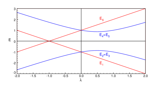
Figure 1: Eigenvalues of the matrix (1)

Figure 2: Graphical representation of the matrix (1)

References

- [1] J. J. Sylvester, On a remarkable discovery in the theory of canonical forms and of hyperdeterminants, The London, Edinburgh, and Dublin Philosophical Magazine and Journal of Science. Series 4 2 (1851) 391-410.
- [2] H. B. Griffiths, Cayley’s Version of the Resultant of Two Polynomials, Am. Math. Month. 88 (1981) 328-338.
- [3] S. Basu, R. Pollack, and M.-F. Roy, Algorithms in Real Algebraic Geometry, Second (Springer-Verlag, Berlin, (2003).
- [4] W. D. Heiss and W. -H. Steeb, Avoided level crossings and Riemann sheet structure, J. Math. Phys. 32 (1991) 3003-3007.
- [5] V. V. Stepanov and G. Müller, Integrability and level crossing manifolds in a quantum Hamiltonian system, Phys. Rev. E 58 (1998) 5720-5726.
- [6] T. J. Davis, 2 D magnetic traps for ultra-cold atoms: a simple theory using complex numbers, Eur. Phys. J. D 18 (2002) 27-36.
- [7] I. Freund, Coherency matrix description of optical polarization singularities, J. Opt. A 6 (2004) S229-S234.
- [8] W. D. Heiss, F. G. Scholtz, and H. B. Geyer, The large N behaviour of the Lipkin model and exceptional points, J. Phys. A 38 (2005) 1843-1851.
- [9] M. Bhattacharya and C. Raman, Detecting Level Crossings without Looking at the Spectrum, Phys. Rev. Lett. 97 (2006) 140405.
- [10] M. Bhattacharya, How to detect level crossings without looking at the spectrum, Am. J. Phys. 75 (2007) 942-946.
- [11] M. Bhattacharya and C. Raman, Detecting level crossings without solving the Hamiltonian. I. Mathematical background, Phys. Rev. A. 75 (2007) 033405.
- [12] M. Bhattacharya and C. Raman, Detecting level crossings without solving the Hamiltonian. II. Applications to atoms and molecules, Phys. Rev. A 75 (2007) 033406.
- [13] A. T. Kotvytskiy and S. D. Bronza, Quasi-analytical method for images construction from gravitational lenses, Odessa Astron. Pub. 29 (2016) 31-33.
- [14] A. Szabo and N. S. Ostlund, Modern Quantum Chemistry, Dover Publications, Inc., Mineola, New York, (1996).
- [15] F. M. Fernández, On the crossing of the energy levels of a parameter-dependent quantum-mechanical Hamiltonian, J. Math. Chem. 25 (2014) 2322-2329.
- [16] M Tinkham, Group Theory and Quantum Mechanics, McGraw-Hill, New York, (1964).
- [17] F. A. Cotton, Chemical Applications of Group Theory, Third (John Wiley & Sons, New York, (1990).
- [18] WikipediA, Resultant and Discriminant, https://en.wikipedia.org/wiki/Resultant, https://en.wikipedia.org/wiki/Discriminant
- [19] J. Böhm, Chronicle of Resultant and Discriminant, The Derive Newsletter 107 (2017) 6-21.