Handling Nonmonotone Missing Data with Available Complete-Case Missing Value Assumption
Abstract
Nonmonotone missing data is a common problem in scientific studies. The conventional ignorability and missing-at-random (MAR) conditions are unlikely to hold for nonmonotone missing data and data analysis can be very challenging with few complete data. In this paper, we introduce the available complete-case missing value (ACCMV) assumption for handling nonmonotone and missing-not-at-random (MNAR) problems. Our ACCMV assumption is applicable to data set with a small set of complete observations and we show that the ACCMV assumption leads to nonparametric identification of the distribution for the variables of interest. We further propose an inverse probability weighting estimator, a regression adjustment estimator, and a multiply-robust estimator for estimating a parameter of interest. We studied the underlying asymptotic and efficiency theories of the proposed estimators. We show the validity of our method with simulation studies and further illustrate the applicability of our method by applying it to a diabetes data set from electronic health records.
Keywords: nonmonotone missing data, missing not at random,inverse probability weighting, regression adjustment, multiply-robustness
1 Introduction
Missing data problems are very common in scientific research (Molenberghs et al., 2014; Little and Rubin, 2019). Based on the missing/response patterns, these problems can be categorized into monotone and nonmonotone missing data problems. For monotone missing data, variables subject to missing are ordered and if one variable is missing, all subsequent variables are missing. This occurs when individuals drop out of a study, which is common in longitudinal studies (Diggle et al., 2002). Nonmonotone missingness refers to the case when no such ordering exists (Molenberghs et al., 2014; Little and Rubin, 2019). For example, a participant might drop out and later return to a study. Nonmonotone missingness may also occur for regression analysis when outcomes and predictors are missing under arbitrary patterns.
Handling nonmonotone missing data is a very challenging task even if we assume missing-at-random (MAR) (Robins and Gill, 1997; Sun and Tchetgen Tchetgen, 2018). Inverse probability weighting (IPW) estimator for nonmonotone missing data may also be unstable under MAR (Sun and Tchetgen Tchetgen, 2018). Further, Robins and Gill (1997) and Vansteelandt et al. (2007) have argued that the MAR restriction should not be expected to hold in nonmonotone missing data.
In this paper, we are interested in dealing with nonmonotone missing data that are missing-not-at-random (MNAR). Our study is motivated by an electronic health records (EHRs) data set that contains longitudinal information of diabetes patients. For patients with diabetes, one important variable is the glycated hemoglobin (HbA1c) measurement and a controlled HbA1c level () is known to reduce the risk of microvascular complications. However, EHR data also poses significant challenges. EHR data are incomplete as a patient’s information is recorded only if and when they visit a clinic. This naturally leads to nonmonotone missing data when a patient reappeared after one or more missed visits. Another complication is that the missing patterns of HbA1c are associated with the underlying HbA1c levels. For example, sicker patients with higher HbA1c levels are likely to visit clinics often and thus have less missing values, while healthier patients are likely to miss visits and thus have more missing values. This suggests that the HbA1c missing mechanism is MNAR. Thus, we have nonmonotone and MNAR data for the HbA1c measurements.
The diabetes EHR data set contains 8663 patients who were enrolled from 2003 to 2013, and who were followed up every 3 months until the 4th quarter of 2013. Thus, the longest follow up time is 11 years (44 quarters). For the purpose of this paper, we will focus on first-year’s data and define as the HbA1c measurement for the -th quarter with and as the baseline measurement. There are three main questions we would like to address:
-
•
Q1. Single variable of interest. Given first-year’s data (), we are interested in estimating the mean HbA1c levels at the 4-th quarter, i.e., .
-
•
Q2. Multiple variables of interest: summary measures. Given first-year’s data, we want to estimate the probability that a patient successfully controls the HbA1c levels below 7% for the 3rd and 4th quarters, i.e., . Further, we are also interested in estimating the averages of the HbA1c levels for the last two quarters, i.e, .
-
•
Q3. Multiple variables of interest: marginal parametric model. Given first-year’s data, we want to study the linear relationship between and , i.e., we want to estimate the following linear regression model:
Addressing these questions is a non-trivial problem because we have nonmonotone missingness in the data and the missingness is MNAR. Several attemps have been made to handle nonmonotone missing data that is MNAR. One approach is to assume specific parametric models for both the study variables and the missing probability (Troxel et al., 1998a, b; Ibrahim et al., 2001). Another approach is the no self-censoring or itemwise conditionally independent nonresponse restriction (Shpitser, 2016; Sadinle and Reiter, 2017; Malinsky et al., 2021) and a variant of this idea is the causal graph approach (Nabi et al., 2020; Mohan and Pearl, 2021). Robins and Gill (1997) proposed the group permutation model and Zhou et al. (2010) proposed the block conditional MAR model. Little (1993) and Tchetgen et al. (2018) considered the complete-case missing value (CCMV) restriction. Tchetgen et al. (2018) used discrete-choice models to generate a class of MNAR assumptions. Linero (2017) introduced the transformed-observed-data restriction which requires specifying a transformation and it is also a partial identifying restriction. Chen (2022) introduced the idea of a pattern graph to generate further MNAR assumptions. However, all these existing work have limitations and cannot be applied to our problem. The no self-censoring restriction requires that no variable can be a direct cause of its own missingness status, which is unlikely to be true for the diabetes EHR data that we are investigating. Other methods such as the CCMV and pattern graph rely heavily on the size of the complete cases. However, for the first year’s data , complete cases only account for of the observations in our data set.
In this paper, we introduce a useful identifying assumption called available complete-case missing value (ACCMV) assumption for handling nonmonotone missing data that is MNAR. In practice we often have many variables at hand and only a few of them are of primary interest. We call them primary variables. For those auxillary variables that are not of direct interest, they are often correlated with the primary variables and the missing mechanism of the primary variables. Thus they can be used to assist with the estimation for primary variables. For Q1 of the diabetes example, are auxillary variables and is the primary variable. We can use to help with the estimation of . In such a scenario, the conventional CCMV assumption will require all the variables to be fully observed for identification. However, requiring auxillary variables to be fully observed is a strong condition to identify parameters that only involve the primary variable. Ideally, we should also use those observations with primary variables fully observed and auxillary variables partially observed for identification.
On a high level, the principle of ACCMV imposes an assumption similar to the CCMV on the primary variables for identification and an assumption similar to the available-case missing value (ACMV) assumption (Molenberghs et al., 1998) on the auxillary variables to improve the effective sample size. This allows a much larger set of observations to be used for identification. For the diabetes example, close to 48% of the patients have observed, while only 5% of the patients have fully observed. Thus, CCMV will only use 5% of the observation for identification and ACCMV instead will use 48% of the observations for identification. For this reason, ACCMV is particularly suitable for analyzing data sets with few complete cases.
Outline. In Section 2, we introduce the relevant notations. In Section 3, we study the case with single primary variable. We show that ACCMV assumption leads to nonparametric identification of the distributions for the primary variable and develop an IPW estimator, regression adjustment estimator and a multiply-robust estimator. In Section 4, we extend our analysis to multiple primary variables and study the identification, estimation procedure and efficiency theory. We conduct a case study to investigate the scenario of marginal parametric models in Section 5. Section 6 studies the problem of sensitivity analysis of the ACCMV assumption. We conduct simulation studies in Section 7 and apply our approach to the diabetes data set in Section 8. All the code for our experiments is available at https://github.com/mathcg/ACCMV.
2 Notations
In our analysis, we divide all the variables into two sets: a set of variables called primary variables, denoted as , and another set of variables called auxillary variables, denoted as . We are interested in structures involving the primary variables . The auxillary variables are not of primary interest and mainly help with the estimation involving the primary variables. Namely, the parameter of interest is a statistical functional of and does not involve . We cannot ignore in our analysis because may be related to the missing data mechanism of . We use to denote the norm such that for a vector , we have . Further, we use to denote the norm as .
Both and are subject to missingness. We use the binary vector to denote the response pattern of , i.e., if is observed and to denote the response pattern of , i.e., if is observed. We use the notation and to denote the observed parts of and under pattern . Let and . We use the notation and to denote the vector after flipping and in and , respectively. The variable and will then refer to the missing variables under pattern and . We further define if for . For instance, but cannot be compared with .
Take the diabetes EHR data as an example. For question Q1 in Section 1, the primary variable is and the auxillary variable is . Suppose we only observe , then this individual would have response patterns and . For question Q2, our primary variables is and the auxillary variables . For the individual who we only observe , the response pattern is and . In what follows, we will give concrete examples of what ACCMV assumption stands for in different contexts.
3 Single Primary Variable for ACCMV: Estimation and Inference
To start with, we consider a simple scenario where we only have one primary variable (), i.e., and , and we are interested in estimating the mean functional for some known function . For the diabetes EHR data, this occurs when we are interested in estimating the average value of the HbA1c measurement at the end of the first year, i.e., and . A straightforward calculation shows that
Clearly, is identifiable and can be estimated by a simple sample mean, i.e., , so we focus on identifying the second term . We can show that
The quantity is identifiable from the data. So the key is to identify the first component , which is also known as the extrapolation density.
The conventional CCMV assumption will impose the assumption
| (1) |
While equation (1) identifies the parameter , it has a limitation that all the information relies on the complete case . For the diabetes data set, only a very small fraction (5%) of the patients have fully observed. So the CCMV might lead to an unreliable estimate.
The ACCMV is based on the insight that the complete case of is enough for identifying the parameter of interest and we should be more flexible about the response patterns for the auxillary variables . Formally, the ACCMV assumption imposes the following assumption:
| (2) |
Namely, to identify under pattern , we use any patterns as long as the primary variable is observed and the same set of auxillary variables are also observed. The assumption (2) allows the use of a much larger set of observations to infer the information in variable . We can further prove that ACCMV assumption leads to nonparametric identification (Robins et al., 2000) of the marginal distribution and this assumption will not conflict with the observed data.
Proposition 1
Under the ACCMV assumption in equation (2), is nonparametrically identified.
It is immediate from Proposition 1 that is identifiable under the ACCMV assumption.
Example 1
Consider the example where we have auxillary variables and we focus on the pattern and . The CCMV will assume that
and the ACCMV will assume that
For CCMV, the extrapolation density is estimated by observations with whereas in the ACCMV, the extrapolation density is estimated by observations with . Clearly, ACCMV allows us to estimate with a much larger set of observations, leading to a more reliable estimate.
3.1 IPW Estimation
Instead of directly estimating , we now propose an IPW approach to estimate .
Lemma 2
The ACCMV assumption (2) can be equivalently written as follows.
| (3) |
Lemma 2 suggests that the ACCMV can be expressed as requiring the odds to be independent of the variable .
An important implication from Lemma 2 is that the quantity is identifiable and we can estimate by assuming a parametric model. For example, If we set , the odd can be estimated by simply fitting a logistic regression with covariates that treats pattern as class 1 and patterns as class 0. Let be the estimated version of , where is the estimated parameter.
Next, with equation (3), we can rewrite as an identifiable quantity as follows
| (4) | ||||
This leads to the following IPW estimator:
Combining with the estimator , our final estimator for will be
| (5) |
The expression in the last equality shows an elegant form–we can express IPW estimator as weighting the complete cases with weight and we have the following asymptotic theory for .
Theorem 3
Under the ACCMV assumption in equation (3) and assume that for every ,
for some function such that , and the true odds . We assume that is differentiable with respect to and
for for some . Then
for some .
We can compute the variance either through its influence function or use bootstrap. More specifically, we have
and we can estimate with
where . The form of the influence function can be found in Appendix A. In practice, we recommend bootstrap for its simplicity.
Assumptions in Theorem 3 are mild. The asymptotic linear form of is very common when we use a parametric model and estimate the parameter via the maximum likelihood estimation (MLE). The condition on the gradient of odds is also very mild. For conventional methods such as the logistic regression, this condition holds with covariates that have a bounded second order moment. The condition on the product of and odds is also mild. This condition is required for to have a bounded variance. Alternatively we may make the assumption that is bounded by a large constant for any and . This is very similar to the positivity assumption in the IPW literature.
3.2 Regression Adjustment Estimation
The ACCMV assumption in equation (2) leads to the following identification of :
where
| (6) |
is the outcome regression model. Thus, we can estimate by imposing a model and estimate via using observations with . For instance, we may regress the response versus covariate from observations with . Having estimated , we then construct the estimator
and the final estimator for will be
| (7) |
and we have the following asymptotic theory for .
Theorem 4
Under the ACCMV assumption in equation (2) and assume that for every ,
for some function such that , and the true regression function is . Also, we assume that is differentiable in and
for for some . Then
for some .
Assumptions in Theorem 4 takes a similar form as the ones in Theorem 3. These are mild modeling conditions. If we use a least square approach to fit the parameter and the true parameter indeed solves the least square equation (occurs when the model is correct), then the asymptotic linear form exists. For linear regression, the gradient condition easily holds when the covariates has bounded second moments.
3.3 Semi-parametric Theory and Multiply-robust Estimation
It is known that the IPW and regression adjustment may not lead to an efficient estimator. In this section, we investigate the efficiency theory under the ACCMV assumption. Since and the first component is directly identifiable, we only need to study the efficiency theory of estimating .
Theorem 5
Under the ACCMV assumption, the efficient influence function of estimating is
Based on Theorem 5, the efficient estimator of is
which leads to the estimator
| (8) |
where . The two estimated functions and are the estimators of the regression function and odds . We may use the same estimators as in Section 3.1 and 3.2. We make the following technical assumptions:
Assumptions:
-
(S1)
For each , is in a Donsker class and is in another Donsker class . There exist functions and such that
-
(S2)
are uniformly bounded by a large constant for all .
Assumption (S1) states that estimators and should converge to fixed functions. The Donsker condition is a common condition that controls the complexity of the estimators. Assumption (S2) is a technical condition and can be relaxed by stronger moment conditions on each function. being bounded is related to the positivity assumption in the IPW literature and it is sensible to have also bounded as it estimates . Further, (S2) holds when these functions are smooth and stay in compact sets. The estimator has the following multiply-robustness properties.
Theorem 6
Under the ACCMV assumption, (S1), (S2) and appropriate assumptions for and that we define in Appendix B, the estimator in equation (8) satisfies the following properties:
-
•
Consistency. when
-
•
Asymptotic normality. when
The quantity is the efficiency bound.
The first statement in Theorem 6 states that as long as for each pattern , either the regression estimator or the odds estimator is consistent, the estimator will be consistent. This is known as the multiply-robust property. The second statement states that if both nuisance functions ( and ) are correctly specified and can be estimated sufficiently fast for all patterns , the final estimator will be asymptotically normal and achieve the efficiency bound. The Donsker conditions might be relaxed if sample splitting is employed for estimation of and .
Further, if we can assume that both and are parametric functions, we are able to obtain asymptotic normality as long as either or for each .
Corollary 7
Under the ACCMV assumption and assuming that and are parametric functions for all . We further assume that
Then if or for each , we have
When and for each , we have .
We can either estimate the variance through the influence functions or use bootstrap. The form of the influence functions can be found in Appendix B. In practice, we recommend using bootstrap to compute the confidence intervals for its simplicity.
4 Multiple Primary Variables for ACCMV: Estimation and Inference
Now we consider the problem when is multivariate. As mentioned before, this occurs when we are interested in the last two HbA1c measurements for the first year. In this case, we have and . We assume that the parameter of interest is for some known function . Multiple primary variables also occur in the marginal parametric models, which we will have an in-depth discussion in Section 5.
When we have multiple primary variables, the complete-case that identifies the variable will be . Thus, for , the ACCMV assumption in equation (2) will be revised as
| (9) |
which is equivalent to
| (10) |
Proposition 8
Under the ACCMV assumption in equation (9), is nonparametrically identified for any .
Proposition 8 shows that the ACCMV assumption for multiple primary variables nonparametrically identifies the marginal density . So it is an assumption on the missing data without putting any constraints on the observed data. Our goal is to identify when our data is a collection of IID random elements for .
4.1 IPW Estimation
For any function , we have
When , is identifiable. When , through similar derivations as in (4), we have
and the right hand side is clearly identifiable as long as we can estimate .
Moreover, we have the following equality holds,
with
| (11) |
We can then rewrite the above equality as
The quantity behaves like the weight of observation with .
Based on the above analysis, our estimation procedure of will be the following three-step approach:
-
1.
Step 1: estimating individual odds . We first estimate for . This can be done with a simple logistic regression, i.e., where is estimated by comparing pattern versus using variables .
-
2.
Step 2: computing total weights . For each pattern , we compute
(12) -
3.
Step 3: applying the IPW approach. The final estimator is
(13)
Theorem 9
Under the assumption (10) and assume that for every and ,
for some function such that and . The true odds . We assume that is differentiable with respect to and
for for some . Then
for some .
The conditions in Theorem 9 are very similar to the single primary variable case (Theorem 3). The difference is that here we have multiple response patterns of that we need to consider. Again, assuming the logistic regression model (log odds is linear) is correct, then all these assumptions hold whenever and have bounded second moments. The proof can be found in Appendix C and the variance can be estimated either through the influence function or bootstrap.
4.2 Regression Adjustment Estimation
Similar to the case of single primary variable scenario, we may apply a regression adjustment approach to estimate as well. The idea is based on the pattern mixture model formulation in equation (9) that links the extrapolation density to an observed density.
Specifically, for , Equation (9) implies that the parameter can be expressed via the following form:
where
| (14) |
is the outcome regression model. As a result, the regression adjustment approach leads to the following two-stage estimator of :
-
1.
Step 1: estimating the outcome regression. For each with , we estimate via an estimator using observations with and variables . This can be done by placing a parametric model and estimating the underlying parameter .
-
2.
Step 2: regression adjustment. With the estimates from step 1, our final estimate will be
(15)
The regression adjustment estimator can be interpreted as follows. When we have a complete observation of the primary variable (), we observe . When any entries of is missing, we find a proper model based on the response pattern in , together with the response pattern in , and compute the predicted value of .
Theorem 10
Under the assumption of equation (9) and assume that for every ,
for some function such that and . Further, assume that the true regression , is differentiable in and
for for some . Then
for some .
Conditions in Theorem 10 is similar to the conditions in Theorem 4 except that is multivariate. The modeling conditions are also mild; linear regression models will satisfy them when we have bounded second moments of both and . The proof can be found in Appendix C and the variance can be computed either based on the influence functions or bootstrap.
4.3 Semi-parametric Theory and Multiply-robust Estimation
Both IPW and regression adjustment are known to be inefficient. To improve the efficiency of the estimator, we first derive the efficient influence function of .
Theorem 11
Under the ACCMV assumption in equation (10), the efficient influence function of estimating when is
The above theorem implies that we can construct an efficient estimator using the following approach:
| (16) | ||||
where and are estimators of the odds in equation (10) and the outcome regression in equation (14), respectively. We make the following technical assumptions: Assumptions:
-
(M1)
For each and , is in a Donsker class and is in a Donsker class . There exist functions and such that
-
(M2)
are uniformly bounded by a large constant for all and .
Assumptions (M1) and (M2) are multivariate versions of (S1) and (S2).
Theorem 12
Under the ACCMV assumption (9), (M1), (M2) and appropriate assumptions for and that we define in Appendix C, the estimator has the following properties:
-
•
Consistency. when
-
•
Asymptotic normality. when
The quantity is the efficiency bound.
Theorem 12 implies that the estimator is multiply-robust in the sense that as long as we have either or being consistently estimated for all and , the estimator will be consistent. Further it achieves the efficiency bound when the two sets of nuisance models are estimated sufficiently fast.
5 Multiple Primary Variables for ACCMV: Marginal Parametric Model
In practice, we often impose a marginal parametric model over the primary variable and use the data to estimate the underlying parameter. To start with, we consider two motivating examples.
Example 2
(Modeling the marginal distribution) We assume that , where is a known parametric distribution such as a multivariate Gaussian, and the goal is to estimate the underlying parameter . A typical approach to estimate is the maximum likelihood estimator (MLE). Under usual regularity conditions, the true parameter solves the population score equation:
When there is no missingness in , the MLE is obtained from the following sample score equation:
To give a concrete example of this, consider again the one-year diabetes data . Suppose that we are interested in the joint distribution of the last two visits, i.e., , and we assume that it follows a bivariate Gaussian, i.e., , where is the mean vector and is the covariance matrix. Then we can easily estimate and using the MLE.
Example 3
(Modeling the marginal moment restricted model) It is also very common that the parameter of interest may be a moment restricted model among variables in . For instance, we may impose a linear model , where is all variables in except the first one (for simplicity, we ignore the intercept). The parameter of interest is the regression coefficient . In this case, we often estimate the parameter by the least square approach, i.e., at the population level, the parameter satisfies
or equivalently, the parameter solves the following equation:
When there is no missingness in , the least square estimate solves the following estimating equation
In the diabetes data, if we are interested in the linear relationship among and , we can use the model above and treat and .
In both examples, we see that the parameter of interest is now defined through a population estimating equation
| (17) |
So we will focus on the case of parameters defined through an estimating equation, and how to obtain a consistent estimate when there are missingness in based on the ACCMV assumption (10).
5.1 IPW Marginal Parametric Model
The IPW approach in Section 4.1 can be easily adopted to the marginal parametric model. Specifically, the population estimating equation of (17) can be written as
| (18) | ||||
where the weight function is from equation (11).
As a result, the three-step procedure in Section 4.1 can be applied here with a mild modification:
-
1.
Step 1: estimating individual odds . For and , we first estimate . This can be done by a simple logistic regression, i.e., where is estimated by comparing pattern versus using variables .
-
2.
Step 2: computing total weights . For each pattern , we compute its total weight
-
3.
Step 3: solving the weighted estimating equation. The final estimator is from
(19)
The first two steps are the same as Section 4.1. We only need to modify the last step by solving a weighted estimating equation. We have the following asymptotic results for .
Theorem 13
Under assumption (10) and assume that for every and ,
for some function such that and . The true odds . Next we assume that is differentiable in and
for for some . Further we assume that
exists and is invertible. Assuming that , we have
for some covariance matrix .
5.2 Potential Problems with Regression Adjustment
The marginal parametric model has one distinct property from the general case of multiple primary variables: the regression adjustment method and the multiply-robust approach may be problematic. The main reason is: both regression-adjustment and multiply-robust approach will involve imposing a conditional model on one subset of conditioned on another subset of . This procedure implicitly places a model constraint on the distribution of , which will conflict with the marginal parametric model when the model is not designed well. The multiply-robust estimator also suffers from the same problem since it involves a model on the outcome regression. On the other hand, the odds in the IPW approach is a conditional model on the selection odds , so it is always compatible with the marginal parametric model. Hence, we recommend using the IPW approach in the case of marginal parametric model.
This phenomenon is similar to the model congeniality problem introduced in Meng (1994). The model congeniality problem refers to the case where the imputation model may not be compatible with the analysis model imposed on the imputed data. An imputation model can be viewed as a Monte Carlo approximation to the regression adjustment method and the marginal parametric model on is the analysis model in Meng (1994). Thus, the model conflicting problem we encounter when using regression adjustment on marginal parametric model can be viewed as another form of model congeniality problem.
6 Sensitivity Analysis via Exponential Tilting
The fact that the ACCMV assumption is nonparametrically identified implies that it cannot be tested by the data, which means that it is a weak assumption. However, it is possible that the ACCMV assumption may not be correct or is only approximately correct. The sensitivity analysis (Little et al., 2012) is often conducted to study how the estimate changes when we slightly perturb the underlying missing data assumption.
Here we propose to perform sensitivity analysis of ACCMV via an exponential tilting approach (Kim and Yu, 2011; Shao and Wang, 2016; Zhao et al., 2017). For , recall that the ACCMV in equation (10) requires:
In reality, the odds on the left-hand-side of the above equality may depend on the unobserved value of . Using the concept of exponential tilting, we propose to perturb assumption (10) as follows:
| (20) |
where is a given vector that represents the amount of perturbation from the ACCMV assumption. Clearly, when is a zero vector, equation (20) reduces to the usual ACCMV assumption.
In practice, we will choose a sensitivity parameter vector first, which implies for every . Then based on the perturbation (20), we compute the modified final estimate. For the IPW estimator, We only need to change
in equation (12) to
and change the final estimator in equation (13) to
| (21) |
with . Note that is estimated under assumption (10).
Under a logistic regression model, the sensitivity parameter in the exponential tilting approach (20) has a nice interpretation. Recall that the logistic regression model will model
Thus, equation (20) will become
Each and each element have the same interpretation–they are the coefficient on linear model of the log odds. Consider a specific example that , ( is observed) and the coefficient on is . Then a sensitivity parameter can be interpreted as the effect of the unobserved variable on the log odds is half of the estimated effect of the observed variable . Thus, practitioners can use this as a way to think about a feasible range of the sensitivity parameter .
7 Simulation Study
We now show the validity of our methods with simulation studies. Section 7.1 considers the case when there is a single primary variable. Section 7.2 considers the case when there are multiple primary variables. Section 7.3 applies our ACCMV assumption to a linear regression model.
7.1 Single Primary Variable
We have and and we are interested in estimating . Let be the number of observed variables. Next, we generate data as follows:
-
1.
-
2.
with , , and
Further, we assume that for and . Note that under ACCMV assumption, for are also specified given the data generations above.
We first consider estimation using the regression adjustment method. Under ACCMV, we can compute that and the details are left in Appendix E. We fit linear regression models
for and get . The form of the linear regression models can be found in Appendix E. Then, we can get the estimates using regression adjustment as
Next, we consider the IPW estimates. We can compute the odds functions as follows.
To get the estimate, we fit a logistic regression model
for each and get . Then we can get the estimate using IPW as
For the multiply-robust estimator, we can use the linear regression models and logistic regression models that we fitted before. Then for each , we can get the estimate as
Our final multiply-robust estimator is then
| (22) |
where .
For the multiply-robust estimator, we first consider the case when all the regression functions and odds functions are correctly specified. Next we consider the case when one of the regression function is misspecified. When , the correct regression model is and we fit a linear regression model with only. We also apply the same model misspecification to the regression adjustment estimator. We further consider the case when one of the odds function is mis-specified. When , the correct odds function is and we fit a logistic regression with intercept only. Again we apply the same model misspecification to the IPW estimator. Finally we consider the case when both the regression function and the odds function is incorrect. When , we fit a linear regression model with only and we fit a logistic regression model with intercept only for the odds function.
Table 1 contains the simulation results. We generate 1,000 samples with . The bias is computed as the difference of the average of 1,000 parameter estimates and the true value of . Sample standard error (SE) is computed as the standard error of the 1,000 parameter estimates and the mean theoretical SE is computed as the mean of the 1,000 SE estimates. For all three methods, we estimate the SE for the estimators through their corresponding influence functions111The actual form of the influen functions can be found in Appendix.. Note that bootstrap is an alternative approach to estimate the SE. The sample standard SE reflects the true SE of the estimator and the mean theoretical SE reflects the accuracy of the SE estimated through the influence functions. CI stands for Confidence Interval, RA stands for regression adjustment and MR stands for multiply-robust.
Based on the simulation results, we can see that 95% CI of IPW is undercovering when all the odds function are correctly specified. This is primarily due to the under-estimation of the SE for the IPW estimators in this setup. For this specific data generation setting, the difficulty is that we are estimating the variance of a very heavy-tailed distribution. We can see that the mean theoretical SE is much smaller than the sample SE, which suggests that the estimated SE is much smaller than the true SE. Next, IPW with misspecified odds function leads to much larger bias and even worse coverage for the 95 CI%. We also observe that the mean theoretical SE is much smaller than the sample SE. However, multiply-robust estimator with the same misspecified odds function obtains much better performance. We can see that the bias is very small, the coverage of the 95% CI is very close to the nominal coverage and the difference between mean theoretical SE and the sample SE is also much smaller now. This shows the robustness of the multiply-robust estimator.
Further, regression adjustment achieves nominal coverages and smallest SE estimates when all regression functions are correctly specified. RA with misspecified regression function also leads to large bias and bad coverage for the 95% CI. Again, multiply-robust estimator with the same model misspecification is able to reduce the bias and improve the coverages. We can see that in this case, all multiply-robust estimators underestimate their variances for the same reason as the IPW estimator. However, the coverages of the 95% CI are much better for multiply-robust estimators compared to the IPW estimator. When both the regression and odds function are misspecified, the multiply-robust estimator also obtained biased estimates and bad coverages for the 95% CI. Finally, we also include the results estimating using complete-case analysis. It is clear from the simulations that under ACCMV assumption, the data is missing-not-at-random as complete-case analysis is severely biased.
| Methods | Bias | Sample SE | Mean theoretical SE | Coverage of 95% CI |
|---|---|---|---|---|
| IPW | -0.006 | 0.216 | 0.113 | 0.778 |
| IPW (incorrect) | -0.084 | 0.174 | 0.090 | 0.536 |
| RA | -0.001 | 0.044 | 0.043 | 0.955 |
| RA (incorrect) | 0.040 | 0.045 | 0.046 | 0.857 |
| MR (correct) | -0.002 | 0.105 | 0.072 | 0.931 |
| MR (IPW incorrect) | 0.000 | 0.069 | 0.057 | 0.939 |
| MR (RA incorrect) | -0.000 | 0.118 | 0.074 | 0.920 |
| MR (Both incorrect) | 0.041 | 0.069 | 0.058 | 0.870 |
| Complete Case | -0.178 | 0.035 | 0.034 | 0.001 |
7.2 Multiple Primary Variables
We have and . The parameter of interest is and this allows the estimation of the given and . For any , let be the number of observed primary variables. We generate the data as follows.
-
1.
for .
-
2.
for any and any .
-
3.
for any .
where , and
Further, we also assume that for and .
We first consider regression adjustment method. Under the ACCMV assumption, we can compute and the details can be found in Appendix E. Now to get the estimate, we need to fit the following regression models:
for . Note that equivalently we can fit the following regression models
for and get . The actual form of the regression models can be found in Appendix E and we have
Then we can get the estimate using regression adjustment as
Next, we consider the IPW estimation. It is not hard to get that for , is a linear function of and . Then we can fit a logistic regression model as follows:
for each , and get . We can get the estimate using IPW as
We now consider the multiply-robust estimation. We can get the estimate using the following multiply-robust estimator
with the same estimators and as before. Again, we consider the case when all the regression functions and odds functions are correctly specified. Next, we consider the case when two of the regression estimators is misspecified. When and , the true regression model is and we fit a linear regression with intercept only. When and , the true regression model is and we also fit a linear regression model with intercept only. We apply the same model misspecification to the regression adjustment estimator. Further, we consider the case when two of the odds function are misspecified. When and , the true odds function is and we fit a logistic regression with intercept only. When and , the true odds function is and we also fit a logistic regression with intercept only. We also apply the same model misspecification to the IPW estimator. Finally, we consider the case when both the regression function and the odds function are misspecified. When and , we fit a linear regression model with intercept only for the regression function and we also fit a logistic regression model with intercept only for the odds function. When and , again we fit linear regression and logistic regression models with intercepts only.
| Methods | Bias | Sample SE | Mean theoretical SE | Coverage of 95% CI |
|---|---|---|---|---|
| IPW | -0.000 | 0.075 | 0.074 | 0.943 |
| IPW (incorrect) | 0.078 | 0.079 | 0.079 | 0.852 |
| RA | -0.001 | 0.065 | 0.066 | 0.956 |
| RA (incorrect) | -0.048 | 0.065 | 0.068 | 0.892 |
| MR (correct) | -0.001 | 0.066 | 0.066 | 0.948 |
| MR (IPW incorrect) | -0.001 | 0.065 | 0.066 | 0.949 |
| MR (RA incorrect) | -0.001 | 0.067 | 0.067 | 0.952 |
| MR (both incorrect) | 0.014 | 0.068 | 0.065 | 0.943 |
| Complete Case | 0.131 | 0.092 | 0.092 | 0.723 |
From table 2, we can see that IPW, RA and multiply-robust estimators all obtained close to 0 bias and achieves nominal coverages for the 95% CIs when the regression or odds functions are correctly specified. In comparison, we also observe that IPW estimator obtained relatively large SE estimates, while multiply robust estimators and regression adjustment estimator obtained relatively similar SE estimates. As expected, both IPW and regression adjustment estimators fails when the regression or odds functions are misspecified. Multiply-robust estimators with the same model misspecification are able to achieve nominal coverages and small biases. Further, when both the regression and odds functions are misspecified, multiply-robust estimators obtain relatively large bias. Finally, the complete-case analysis again obtained severely biased estimates.
7.3 Marginal Parametric Model
In this section, we consider the following setup for the marginal parametric model. We have and . We want to estimate the following linear regression model
Further, we assume that
-
1.
with and
-
2.
for .
-
3.
for .
-
4.
.
with being the normalization term. It can be verified that this data generation satisfies the ACCMV assumption. Given the data generation above, we have
As discussed in section 5, we will be using IPW to estimate the parameters for the linear regression model. We can estimate individual odds by fitting a logistic regression model as follows:
and get . Next, we compute the total weights for each such that
Finally, we can get by solving the following weighted estimating equation:
From table 3, we can see that IPW gives close to 0 bias and achieves nominal coverage for the 95% confidence intervals. On the other hand, complete-case analysis obtained biased estimates.
| Bias (SE) | Coverage of 95% CI | |||
|---|---|---|---|---|
| Methods | ||||
| IPW | -0.001 (0.039) | -0.001 (0.046) | 0.949 | 0.938 |
| Complete Case | -0.061 (0.042) | -0.008 (0.043) | 0.725 | 0.943 |
8 Applications to the Diabetes Data
We apply the proposed estimation procedures to the diabetes EHR data set, assuming that ACCMV holds. This data set contains 8663 patients who were followed up every 3 months from 2003 to 2013.
8.1 Summary Measures of the HbA1c Levels
We focus on the HbA1c levels measured from the baseline and the first year, . We now answer the first two questions raised in the introduction. We estimate
-
1.
The mean HbA1c levels at the end of the first year, .
-
2.
The proportion of patients that have their HbA1c levels controlled, meaning that their HbA1c levels are below 7%, i.e., . 222For convenience, we multiply the value of HbA1c levels by 100.
-
3.
The averages of the HbA1c levels for the last two quarters, .
For the estimation of , the primary variable is and the auxillary variables are . For the estimations of and , the primary variables are and the auxillary variables are .
We construct the 95% confidence intervals using bootstrap. The results are given in Table 4 and 5. We can see that IPW, regression adjustment and multiply robust estimators all obtain quite similar results. The only exception is with the estimation of , where IPW and multiply-robust estimators obtain non-overlap 95% confidence intervals. This could be due to the incorrect specifications of the odds functions. We can also see that results of complete-case analysis are different from the rest three methods. Complete-case analysis tends to over-estimate the HbA1c levels. This suggets that the missingness of HbA1c is relevant to the underlying values of HbA1c, which agrees with the intuition that healthier patients are more likely to miss their HbA1c measurements.
More specifically, our ACCMV approach shows that both and is less than 7 and more than 50% of the participants have their HbA1c levels controlled for the last two quarters; while complete-case analysis obtain completely opposite results. This highlights the importance of treating missing data in a real data set.
| Methods | |||
|---|---|---|---|
| IPW | 6.927 (6.897 - 6.956) | 0.534 (0.515 - 0.556) | 6.931 (6.900 - 6.958) |
| Regression Adjustment | 6.936 (6.907 - 6.966) | 0.569 (0.554 - 0.583) | 6.955 (6.925 - 6.983) |
| Multiply Robust | 6.931 (6.902 - 6.960) | 0.575 (0.559 - 0.589) | 6.949 (6.920 - 6.976) |
| Complete Case | 7.011 (6.974 - 7.049) | 0.454 (0.431 - 0.477) | 7.197 (7.143 - 7.252) |
8.2 Sensitivity Analysis
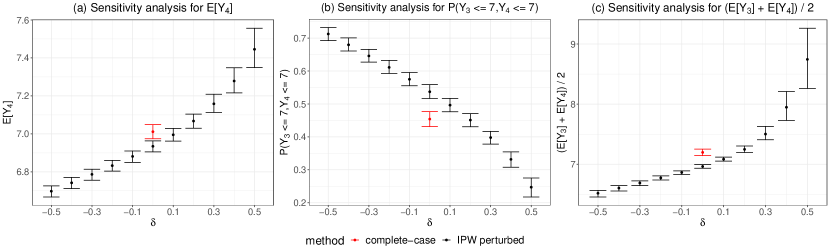
We also perform sensitivity analysis by the exponential tilting approach proposed in section 6. We use the same sensitivity parameter for all patterns, i.e., every element of in equation (21) is identical. From a practical perspective, we modify the exponential tilting as . This allows the missingness of HbA1c measurements to follow the intuition that a healthier patient with controlled HbA1c levels are more likely to miss their HbA1c measurements, while a sick patients are less likely to miss their HbA1c measurement. For example, with a negative , is more likely to be positive for healthier patients (because their HbA1c levels are more likely to be less than 7) and thus increase the missing probability. Similarly, a negative will decrease the missing probability for sicker patients. For completeness, we also displays the results with a positive , which will reverse the relationship between health status and HbA1c missing probability.
Figure 1 show the estimates and 95% confidence intervals for , and as we vary the sensitivity parameter . We can see that the results highly agree with our intuition. When is negative and the magnitude of increases, the mean HbA1c levels decreases as we take into account of the fact that healthier patients with lower HbA1c values are more likely to be missing. For the same reason, the proportion of patients having their HbA1c levels controlled also increases. In the unrealistic scenario that is positive, we observe opposite results.
8.3 Marginal Parametric model
| Methods | |||
|---|---|---|---|
| IPW | 1.120 (0.807 - 1.438) | 0.148 (0.059 - 0.230) | 0.690(0.590 - 0.793) |
| Complete Case | 1.364 (1.127 - 1.601) | 0.104 (0.048 - 0.160) | 0.701(0.645 - 0.758) |
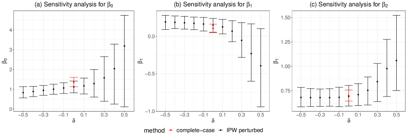
Further, we also want to study the linear relationship between and . Our intuition is to predict , should be more important compared to . We consider estimating the linear regression model as follows:
For the linear regression model, the primary variable is and the auxillary variables are . Table 5 shows that indeed both and has a positive association with and has a stronger association than . Figure 2 shows the estimates and 95% confidence intervals for as varies. We can see that when is negative, the estimates are quite robust and do not change much.
9 Conclusion
In this paper, we introduced the ACCMV assumption to handle nonmonotone and MNAR data. Our ACCMV assumption allows a much larger set of observations to be used for identification compared to the traditional CCMV assumption. Thus, ACCMV is particularly suitable for analyzing data sets with few complete cases. We further proposed IPW, regression adjustment and multiply-robust estimators. We also studied their asymptotic and efficiency theories. We then proposed a sensitivity analysis approach for the ACCMV model for the IPW estimator. Our simulation studies confirm the validity of the assumption. The real data results also highlight the effect of missing data on the final estimate and the importance of efficiently handling the missing data.
So far, we have focused on the first-year’s data for the HbA1c measurements. However, the diabetes patients are followed up to 11 years and a patient could potentially have up to 44 measurements. Thus, it is helpful to also consider longer history of HbA1c measurements as this can provide more information of a patient. In particular, it will be of interest to recover the whole trajectory for a patient who has a bunch of missing values. This is a much more challenging task as the missing patterns increase exponentially when the number of measurements increases. We leave the trajectory recovery problem to future work.
Acknowledgments
We would like to acknowledge support for this project from the National Science Foundation (NSF grant DMS 195278 and 2112907 and CAREER award DMS 2141808) and the National Institute of Health (NIH grant U24 AG072122).
Appendix Appendix A Proof for Single Primary Variable
Proof of Proposition 1. is clearly identifiable. We can write as
and we further have
Thus, is identifiable under ACCMV, which implies that is identifiable.
Proof Of Lemma 2. We have
We start by giving the asymptotic linear expansion of . Given
we have . The log-likelihood has the following form:
The score is
Further, consider such that and assuming that is the unique solutions for . Next, we assume that . Then by theorem 5.9 of Van der Vaart (2000), we have that . Further, we have that
and that with
Under appropriate assumptions (see theorem 5.21 of Van der Vaart (2000)), we have that
where
Proof of Theorem 3. We prove the asymptotic normality of through its asymptotic linear form. For notational convenience, we denote . Then, we have that . We can rewrite as
Term is already in the linear expansion form. For term , we have that
Thus, combined with term , we have
and denote . Then we have with .
Similarly, we first give the asymptotic linear expansion of . The estimating equation for now has the following form:
Again for parametric models, under appropriate assumptions (see theorem 5.9 of Van der Vaart (2000)), we have that . Further, we have that
and that with
Next, we have that
with .
Proof of Theorem 4. Now we give the proof for the regression adjustment estimation. The proof is very similar to proof of Theorem 3. Similarly, denote , we have that
For term , we have
Thus, combined with term , denote
we have
with .
Appendix Appendix B Proof of Multiply-robustness for Single Variable
Proof of Theorem 5. Recall that the IPW formulation for is
and is the true model. We consider a pathwise perturbation such that satisfies
Under , denote as . We derive the EIF using the semi-parametric theory (see section 25.3 of Van der Vaart (2000)), the EIF is a function such that and
Under model , we also have perturbed odds . We denote . Then, a direct computation shows that
Part is already in the form of an EIF. For part , we need to derive . Now we expand the difference as following:
with
Thus, the difference can be rewritten as
Now part can be rewritten as
Thus, combining part and , we conclude that
We first discuss assumptions for the Donsker classes and where we have assumed that and . We denote the norm as
for a probability measure . We assume that satisifies the following uniform entropy condition (Van Der Vaart and Wellner, 1996):
where the supremum of is taken over all finitely discrete probability measures on . is the covering number of class with respect to the norm (see Definition 2.1.5 of Van Der Vaart and Wellner (1996)) and is an envelope function of such that with being the probability measure for . Similarly we can assume that satisfy a same uniform entropy condition with envelop function . We also assume that and are suitably measurable (see Definition 2.3.3 of Van Der Vaart and Wellner (1996)) and . Further, we let and .
Proof of Theorem 6. By assumption (M1), we have and . The true functions are denoted as and . When the models are correct, we have and . The multiply-robust estimator has the following form:
We first consider another estimator that replaces the estimated functions by the true functions in the multiply-robust estimator.
It is not hard to prove that and
where is the efficiency bound for estimating . Further we have that
| (23) | ||||
We first prove the multiply-robust property when the odds are correctly specified and the regression functions are misspecified. Thus, and . Since , we have . Denote and similarly
Then we can write term in (23) for pattern as
Given that , we have as are uniformly bounded. Further, we have
where is a function that does not involve . As is in a Donsker class , we have is also in a Donsker class
by Example 2.10.7 and 2.10.23 of Van Der Vaart and Wellner (1996) and the assumptions we made before this proof. By Lemma 19.24 of Van der Vaart (2000), we then have
realizing that . For term , similarly define
and
Then we can rewrite term in (23) for pattern as
First note that
This implies that term in (23) for pattern can be written as
Then again given that is in a Donsker class and , we have that and is also in a Donsker class by a similar reasoning as before. By Lemma 19.24 of Van der Vaart (2000), we have
This implies that
as . For term , we can similarly define
and . Then is in a Donsker Class by Example 2.10.23 of Van Der Vaart and Wellner (1996). Given that and are uniformly bounded, we have . Then by Lemma 19.24 of Van der Vaart (2000), we have
and
given the assumption that
Above results imply that . By similar reasoning, when we have odds function misspecified and regression function correctly specified, we also have .
When we have both model correctly specified, by a similar proof as above, term has leading term on the order of for each pattern . Similarly, is also . Thus, we have
Finally, for term , by the same proof, we have
assuming that
Together, we have proved that
In fact, when we use parametric estimators for both and , as long as for each pattern , either or , we have the following asymptotic linear expansion for as
with
This will be used when we run the simulation studies.
Appendix Appendix C Proof for Multiple Primary Variables
Now we present the proof for the results when there are multiple primary variables. The proof for Proposition 8 is omitted as it is very similar to the proof in the single variable case.
First, for the IPW estimator, we again give the influence function when we estimate with a parametric model. We have that
where
with
Proof of Theorem 9. The proof is similar to the proof of Theorem 3 and we directly give the results. Denote
and we have
with .
For the regression adjustment method, we have that
where
with
Proof of Theorem 10. The proof is again very similar to the proof of Theorem 4 and we directly give the results. Now we have
Then, we have
with .
Appendix Appendix D Proof for Marginal Parametric Model
Under mild regularity conditions, we can prove that by theorem 5.9 of Van der Vaart (2000).
Proof of theorem 13. The sample estimating equation for the marginal parametric model under the ACCMV assumption is as following:
We can define
then we have
Define
Then we have that
where we also have
based on our assumption. Thus, put everything together and multiply by on both sides of the equation, we have
next, we have that
Further, we have
Now for term (I), we may use Lemma 19.24 of Van der Vaart (2000) to prove that term I is under the condition that lies in a Donsker class. For term III, it is simply by weak law of large numbers. For term II, it is also as . Thus, this implies that
Thus, put everything together, we have that
Next, we have
Next, put everything together, we have
which implies that
Thus, we have the desired asymptotic normality for .
Appendix Appendix E Derivations for Simulation Studies
We first derive with regression adjustment for single variables case. We have that
Thus, we have that . Under ACCMV assumption, we can then identify as follows:
Next, we have that
Under ACCMV assumption, we have that
with . Then we can compute that
Similarly, we have that
Finally, we also have that
Thus, we could compute the parameter of interest as
where and
For IPW estimation of , we first have that
Further, when , we have
Similarly, we have that
Finally, for , we have that
Now we move to the case of multiple primary variables and derive . We have that
Then we have
Next, we have
and
Then we have that
Next, we have
Thus, we now have that
Next, we have that
Thus, we have that
and
Next consider the case , we have
Thus, we have that
and then
Next, we have
Then we have
Thus, we have
Similarly, we have
and we can get that . Thus, we have
Next, we have
and we can get that
Thus, we have
Next consider the case , we have
By symmetry, we have that . Thus, we have that
Next we have
Again similarly, we have that . Thus, we have that
Next, we have
and similarly we have . Thus, we have that
Next, we have that
and similarly we have and we have that
Thus, we could now compute the parameter of interest as
where
Next, when , we have
Next, when , we have
Finally, the results for are identical to . Thus, collecting all the terms, we can get that .
Now we prove that the simulation setup for the marginal parametric model satisfies the ACCMV assumption. For , we have
and we have
Thus for ,
which does not depend on . Next, for , we have
and is the density function for . Thus, we have
and this holds for all . Similarly, we have
Thus, for any ,
References
- Chen (2022) Yen-Chi Chen. Pattern graphs: a graphical approach to nonmonotone missing data. The Annals of Statistics, 50(1):129–146, 2022.
- Diggle et al. (2002) Peter Diggle, Peter J Diggle, Patrick Heagerty, Kung-Yee Liang, Scott Zeger, et al. Analysis of longitudinal data. Oxford university press, 2002.
- Ibrahim et al. (2001) Joseph G Ibrahim, Ming-Hui Chen, and Stuart R Lipsitz. Missing responses in generalised linear mixed models when the missing data mechanism is nonignorable. Biometrika, 88(2):551–564, 2001.
- Kim and Yu (2011) Jae Kwang Kim and Cindy Long Yu. A semiparametric estimation of mean functionals with nonignorable missing data. Journal of the American Statistical Association, 106(493):157–165, 2011.
- Linero (2017) Antonio R Linero. Bayesian nonparametric analysis of longitudinal studies in the presence of informative missingness. Biometrika, 104(2):327–341, 2017.
- Little et al. (2012) Roderick J Little, Ralph D’Agostino, Michael L Cohen, Kay Dickersin, Scott S Emerson, John T Farrar, Constantine Frangakis, Joseph W Hogan, Geert Molenberghs, Susan A Murphy, et al. The prevention and treatment of missing data in clinical trials. New England Journal of Medicine, 367(14):1355–1360, 2012.
- Little (1993) Roderick JA Little. Pattern-mixture models for multivariate incomplete data. Journal of the American Statistical Association, 88(421):125–134, 1993.
- Little and Rubin (2019) Roderick JA Little and Donald B Rubin. Statistical analysis with missing data, volume 793. John Wiley & Sons, 2019.
- Malinsky et al. (2021) Daniel Malinsky, Ilya Shpitser, and Eric J Tchetgen Tchetgen. Semiparametric inference for nonmonotone missing-not-at-random data: the no self-censoring model. Journal of the American Statistical Association, pages 1–9, 2021.
- Meng (1994) Xiao-Li Meng. Multiple-imputation inferences with uncongenial sources of input. Statistical Science, 9(4):538–558, 1994.
- Mohan and Pearl (2021) Karthika Mohan and Judea Pearl. Graphical models for processing missing data. Journal of the American Statistical Association, 116(534):1023–1037, 2021.
- Molenberghs et al. (1998) Geert Molenberghs, Bart Michiels, Michael G Kenward, and Peter J Diggle. Monotone missing data and pattern-mixture models. Statistica Neerlandica, 52(2):153–161, 1998.
- Molenberghs et al. (2014) Geert Molenberghs, Garrett Fitzmaurice, Michael G Kenward, Anastasios Tsiatis, and Geert Verbeke. Handbook of missing data methodology. CRC Press, 2014.
- Nabi et al. (2020) Razieh Nabi, Rohit Bhattacharya, and Ilya Shpitser. Full law identification in graphical models of missing data: Completeness results. In International Conference on Machine Learning, pages 7153–7163. PMLR, 2020.
- Robins and Gill (1997) James M Robins and Richard D Gill. Non-response models for the analysis of non-monotone ignorable missing data. Statistics in medicine, 16(1):39–56, 1997.
- Robins et al. (2000) James M Robins, Andrea Rotnitzky, and Daniel O Scharfstein. Sensitivity analysis for selection bias and unmeasured confounding in missing data and causal inference models. In Statistical models in epidemiology, the environment, and clinical trials, pages 1–94. Springer, 2000.
- Sadinle and Reiter (2017) Mauricio Sadinle and Jerome P Reiter. Itemwise conditionally independent nonresponse modelling for incomplete multivariate data. Biometrika, 104(1):207–220, 2017.
- Shao and Wang (2016) Jun Shao and Lei Wang. Semiparametric inverse propensity weighting for nonignorable missing data. Biometrika, 103(1):175–187, 2016.
- Shpitser (2016) Ilya Shpitser. Consistent estimation of functions of data missing non-monotonically and not at random. Advances in Neural Information Processing Systems, 29, 2016.
- Sun and Tchetgen Tchetgen (2018) BaoLuo Sun and Eric J Tchetgen Tchetgen. On inverse probability weighting for nonmonotone missing at random data. Journal of the American Statistical Association, 113(521):369–379, 2018.
- Tchetgen et al. (2018) Eric J Tchetgen Tchetgen, Linbo Wang, and BaoLuo Sun. Discrete choice models for nonmonotone nonignorable missing data: Identification and inference. Statistica Sinica, 28(4):2069, 2018.
- Troxel et al. (1998a) Andrea B Troxel, David P Harrington, and Stuart R Lipsitz. Analysis of longitudinal data with non-ignorable non-monotone missing values. Journal of the Royal Statistical Society: Series C (Applied Statistics), 47(3):425–438, 1998a.
- Troxel et al. (1998b) Andrea B Troxel, Stuart R Lipsitz, and David P Harrington. Marginal models for the analysis of longitudinal measurements with nonignorable non-monotone missing data. Biometrika, 85(3):661–672, 1998b.
- Van der Vaart (2000) Aad W Van der Vaart. Asymptotic statistics, volume 3. Cambridge university press, 2000.
- Van Der Vaart and Wellner (1996) Aad W Van Der Vaart and Jon A Wellner. Weak convergence. In Weak convergence and empirical processes, pages 16–28. Springer, 1996.
- Vansteelandt et al. (2007) Stijn Vansteelandt, Andrea Rotnitzky, and James Robins. Estimation of regression models for the mean of repeated outcomes under nonignorable nonmonotone nonresponse. Biometrika, 94(4):841–860, 2007.
- Zhao et al. (2017) Puying Zhao, Niansheng Tang, Annie Qu, and Depeng Jiang. Semiparametric estimating equations inference with nonignorable missing data. Statistica Sinica, pages 89–113, 2017.
- Zhou et al. (2010) Yan Zhou, Roderick JA Little, and John D Kalbfleisch. Block-conditional missing at random models for missing data. Statistical Science, 25(4):517–532, 2010.