X-ray spectroscopy in the microcalorimeter era 4: Optical depth effects on the soft X-rays studied with Cloudy

Abstract

In this paper, we discuss atomic processes modifying the soft X-ray spectra in from optical depth effects like photoelectric absorption and electron scattering suppressing the soft X-ray lines. We also show the enhancement in soft X-ray line intensities in a photoionized environment via continuum pumping. We quantify the suppression/enhancement by introducing a “line modification factor ($f_{\rm mod}$).”

If 0 $\leq$ $f_{\rm mod}$ $\leq$ 1, the line is suppressed, which could be the case in both collisionally-ionized and photoionized systems. If $f_{\rm mod}$ $\geq$ 1, the line is enhanced, which occurs in photoionized systems. Hybrid astrophysical sources are also very common, where the environment is partly photoionized and partly collisionally-ionized. Such a system is V1223 Sgr, an intermediate polar binary. We show the application of our theory by fitting the first-order Chandra MEG spectrum of V1223 Sgr with a combination of Cloudy-simulated additive cooling-flow and photoionized models. In particular, we account for the excess flux for O VII, O VIII, Ne IX, Ne X, and Mg XI lines in the spectrum found in a recent study, which could not be explained with an absorbed cooling-flow model.

1 Introduction

The strongest emission lines observed in the soft X-ray spectra of astrophysical plasmas are H-like and He-like lines from elements between carbon and sulfur, and Fe L-shell lines. Such X-ray emitting plasmas can be collisionally-ionized or photoionized. In collisionally-ionized plasma, ionization or excitation events mainly occur due to electron-ion collisions. In photoionized plasma, ionization is dominated by the interaction between photons and ions/atoms. A hybrid of the two types of plasma is also possible, where the cloud is partly collisionally-ionized and partly photoionized.

Line intensity in observed X-ray spectra can be enhanced or suppressed depending on the following factors. If photoionized, lines may be a) enhanced when electrons bound to the ions absorb photons of appropriate wavelength transitioning to higher energy states followed by radiative cascades, also known as continuum pumping, b) suppressed due to optical depth effects. If collisionally-ionized, only optical depth effects suppress lines in the X-ray spectra. In the soft X-ray regime, the optical depth effects leading to line suppression mainly come from photoelectric absorption of line photons or scattering by electrons. Section 2 and Section 3 present more detailed discussion.

The effects of continuum pumping on the optically thin line intensities, the so-called “Case C”, was introduced by Baker et al. (1938) and later discussed by Chamberlain (1953) and Ferland (1999). Their study was later extended to describe “Case D” (Luridiana et al., 2009; Peimbert et al., 2016), the optically thick counterpart of Case C. Recently, Chakraborty et al. (2021) discussed Case C and Case D in view of the future microcalorimeter missions line XRISM and Athena, focusing on line emission from H- and He-like iron.

Optical depth effects on soft X-ray spectra have been previously investigated by Storey & Hummer (1988) and Hummer & Storey (1992), who calculated the recombination line intensities of H-like carbon, nitrogen, and oxygen assuming “Case B” (Baker & Menzel, 1938) and discussed the effects of finite optical depth and dust on H-like ions. Such effects have also been observed in soft X-ray emission spectra. For instance, recent analysis of soft X-ray spectra from Reflection Grating Spectrometer (RGS) onboard XMM-Newton and High Energy Transmission Grating Spectrometer (HETGS) onboard Chandra explored several optically-thick astrophysical sources like cataclysmic variables, novae, ultraluminous X-ray sources, Seyfert galaxies, elliptical galaxies, X-ray binaries, etc (Ramsay & Cropper, 2002; Rauch et al., 2005; Okada et al., 2008; Pintore & Zampieri, 2011; de Plaa et al., 2012; Matzeu et al., 2020; Amato et al., 2021).

As previously mentioned, there have been extensive studies separately discussing the effects of continuum pumping and optical depth effects on X-ray line intensities. The current need is to develop a comprehensive theory that will account for all the atomic processes changing the soft X-ray spectra. This paper aims to present a framework for interpreting the soft X-ray spectra from photoionized and collisionally-ionized plasma using the spectral synthesis code Cloudy (Ferland et al., 2017). A cooling-flow model has been introduced to treat the multi-phase collisionally-ionized systems.

We also show the application of our model on V1223 Sgr, a member of the cataclysmic variable binary star systems called Intermediate Polars. We address the lack of emission from several lower atomic number H- and He-like ions, as mentioned in Islam & Mukai (2021), with additive cooling-flow and photoionized models. However, our model will be applicable for any optically thick source with/without a radiation source.

This paper is the fourth of the series “X-ray spectroscopy in the microcalorimeter era”. The first three papers discussed the atomic processes in a collisionally excited and photoionized astrophysical plasma for H- and He-like iron for a wide range of column densities. Chakraborty et al. (2020a) explored the effects of Li-like iron on the line intensities of four members of the Fe XXV K$\alpha$ complex - x($2^{3}P_{2}\rightarrow 1^{1}S$), y($2^{3}P_{1}\rightarrow 1^{1}S$), z($2^{3}S\rightarrow 1^{1}S$), and w($2^{1}P\rightarrow 1^{1}S$) through Resonant Auger Destruction (RAD, Ross et al., 1978; Band et al., 1990; Ross et al., 1996; Liedahl, 2005) and line broadening effects by electron scattering. Chakraborty et al. (2020b) introduced a novel method of measuring column density from Case A to B (optically thin to thick) transition by comparing the observed spectra by Hitomi with spectra simulated with Cloudy. Chakraborty et al. (2021) established four asymptotic limits- Cases A, B, C, and D for describing the line formation processes in H- and He-like iron emitting in the X-rays. This paper is a continuation of the framework discussed in the first three papers to study the atomic processes affecting the soft X-ray spectrum.

2 line suppression due to photoelectric and electron opacity

Photoelectric absorption of line photons or scattering by electrons can significantly suppress line intensities. Here we present Cloudy calculations of the net emission, demonstrate line suppression due to absorption and scattering, and give simple analytical estimates of the physical processes which suppress the line emission.

Cloudy actually determines the line emission by solving a fully coupled system of equations giving radiative transitions between levels, as originally described in Section III of Rees et al. (1989). The numerical results can be understood by considering the following approximations to the line transfer.

The fraction of photons that survives (which we call $f_{\rm mod}$ or the “line modification factor”) after N scatterings that is subject to photoelectric absorption and electron scattering is determined by the following equation:

$${f_{\rm mod}}=(1-P_{\rm photoelectric}-P_{\rm scattering})^{N},$$ (1)

where N is the mean number of scatterings experienced by a line photon with a line-center optical depth $\tau$ before escaping an optically thick cloud (Ferland & Netzer, 1979):

$$\rm{N}=\frac{{{1.11\tau^{1.071}}}}{{1+{\rm{({log\tau/5.5}})^{5}}}}$$ (2)

$P_{\rm photoelectric}$ is the probability of photoelectric absorption per scattering, and is given by the following ratio of opacities:

$${P}_{\rm photoelectric}=\frac{{{\kappa_{photoelectric}}}}{{\kappa_{total}}}$$ (3)

$P_{\rm scattering}$ is the probability per scattering that a line photon will be scattered off free electrons due to the very large Doppler shift they receive and be removed from the Doppler core of the line (refer to section 7.1 in Chakraborty et al. (2020a) for a detailed discussion):

$${P}_{\rm scattering}=\frac{{{\kappa_{scattering}}}}{{\kappa_{total}}}$$ (4)

where the total opacity is given by

$$\kappa_{total}=\kappa_{line}+\kappa_{photoelectric}+\kappa_{scattering}$$ (5)

For the most part, $f_{\rm mod}$ gives an estimate for the fraction of photons surviving after photoelectric absorption and electron scattering. Figure 1 shows photoelectric absorption opacities ($\kappa_{photoelectric}$) for temperatures between log  T(Kelvin) = 6.2 and log T(Kelvin) = 6.8 and the electron scattering opacity ($\kappa_{scattering}$), assuming a thermal collisional equilibrium at T. A hydrogen density (n(H)) of 1 cm^-3 was assumed, corresponding to an electron density of $\sim$ 1.2 cm^-3, hydrogen and helium being the two most abundant elements in the Universe. The electron scattering opacity was evaluated by multiplying the electron scattering cross section (6.65 $\times$ 10^-25 cm² ) with its density. Scattering is more important at the longer wavelengths and higher temperatures, while absorption is more important at the shorter wavelengths and lower temperatures. Electron scattering opacity has been estimated

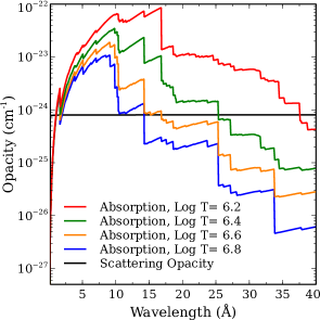
Figure 1: Continuum opacities plotted as a function of wavelength for a cloud with N_H=10²³ cm^-2. Red, green, yellow and blue solid lines show the absorption opacities (photoelectric) for log T=6.2, 6.4, 6.6, and 6.8, respectively. The black solid line shows the electron scattering opacity. The opacity is in units of cm^-1, the unit of opacity appearing in Kirchhoff-Planck law is cm^-1.

Other optical depth effects such as the Case A to B transition and Resonant Auger Destruction can suppress/amplify selected line intensities too (Chakraborty et al., 2020a, b). Numerical Cloudy simulations on optical depth effects shown in this paper include all the atomic processes that can change line intensities. However, we found these effects insignificant compared to photoelectric absorption and electron scattering in the soft X-ray regime. The discussion on the optical depth effects on soft X-ray emission continues in Section 4 for the collisionally-ionized and photoionized cases.

Note that equation 1 applies in collisionally-ionized environments, where there is no external radiation source. In irradiated photoionized environments, $f_{\rm mod}$ will also have contributions from radiative cascades prompted by absorption of line photons from the external radiation source, also known as “continuum pumping”. This is further elaborated in Section 3 and Section 4.2.

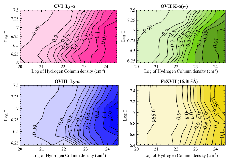
Figure 2: Line modification factors in C VI Ly-$\alpha$, O VII K-$\alpha$ (w), O VIII Ly-$\alpha$, and Fe XVII, in a collisionally-ionized environment, plotted as a function of column density and temperature.

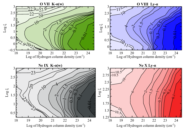
Figure 3: Line modification factor in O VII K-$\alpha$ (w), O VIII Ly-$\alpha$, Ne IX K-$\alpha$ (w), Ne X Ly-$\alpha$, as a function of column density and ionization parameter ($\xi$).

3 line enhancement due to continuum pumping

In photoionized systems, emission lines are enhanced in the presence of external radiation fields due to continuum pumping. Chakraborty et al. (2021) discussed the concept of continuum pumping and its effects in enhancing the line emission from H- and He-like iron. Lines can be enhanced up to $\sim$ 30 times, and the degree of enhancement decreases with the increase in column density due to the optical depth effects, the so-called Case C to D transition. Refer to section 2 in their paper for the mathematical framework of continuum pumping and figure 1 for a simplified three level representation of Case C and Case D.

This work is an extension of the same concept for the soft X-ray regime. The observed spectra (photoionized) will have contributions from line enhancement due to continuum pumping and line suppression due to photoelectric absorption and electron scattering (further discussed in Section 4). Whether the lines are enhanced or suppressed depends on the interplay between these effects. The enhancement/suppression varies with column density/optical depth, ionization parameter ($\xi$), and shape of the incident radiation field. For most of our calculations, we assume a power-law SED:

$$\rm f_{\nu}\propto\nu^{\alpha}$$ (6)

with $\alpha=-1$, except for Section 5 where we let $\alpha$ to vary freely.

4 Optical depth effects on soft X-ray spectra

4.1 Collisionally-ionized emission lines

The practical way to study the effect of optical depth on line intensities is to compute scaled line intensity ratios of a realistic model that includes all the optical depth effects and a simplistic model excluding optical depth effects. The line ratio stands for what fraction of line photons survive.

The realistic model includes absorption and scattering. By default, Cloudy models include absorption but do not include scattering. At X-ray temperatures, a fraction of the line photons gets largely Doppler-shifted from their line-center due to scattering off high-speed electrons. The following Cloudy command reports the line intensities excluding these Doppler-shifted photons:

no scattering intensity

Refer to Section 6 of Chakraborty et al. (2021) for a detailed discussion on no scattering intensity.

In the simplistic model, absorption was switched off with the command:

no absorption escape

The smaller the ratio between the realistic and simplistic model, the larger the suppression. This ratio is the numerical equivalent of $f_{\rm mod}$, the line modification factor, studied in Section 2, which presented an analytical discussion on line suppression in optically thick clouds. Figure 2 shows this ratio for selected soft X-ray lines evaluated with Cloudy.

Temperature and column density are physical parameters that can notably change line emission from the collisionally-ionized cloud. Thus, contour plots have been shown where temperature and column density is varied. Metallicity has been fixed at solar for simplicity. In principle, metallicity should not be taken as a free parameter, as optical depth is proportional to metallicity. This section aims to establish the framework using simplified parameters. In Section 5, we let metallicity vary as a free parameter along with other physical parameters to fit the observed spectrum from V1223 Sgr.

Four panels in the figure show the numerical line modification factor for C VI Ly-$\alpha$ ($\lambda$= 33.736 Å), OVII K-$\alpha$ resonance line (w; $\lambda$=21.602Å), O VIII Ly-$\alpha$ ($\lambda$= 18.969 Å), and Fe XVII ($\lambda$=15.015Å) as a function of the hydrogen column density and temperature for a hydrogen density (n(H)) of 1 cm^-3. There is significant suppression in carbon and oxygen lines and moderate suppression in the iron lines. For example, for CVI Ly-$\alpha$ line at the temperature of its peak emissivity, log T=6.2: at N_H=10²³ cm^-2, the numerical line modification factor as shown in the top-left panel of the figure is $\sim$ 0.15. This implies, only 15 % of the CVI Ly-$\alpha$ line photons will make it out of the optically thick cloud at the mentioned temperature and column density.

Numerical results in the figure account for the full physics and the variation of the physical conditions across the cloud. Analytically, equation 1 estimates the fraction of CVI Ly-$\alpha$ photons surviving after photoelectric absorption and electron scattering, the only two important sources of opacity in the soft X-ray limit.

At the same temperature and column density, $\tau$ $\sim$ 500 (calculated using the Cloudy command save line optical depth), $\kappa_{photoelectric}$= 3.5$\times$ 10^-24 cm^-1, and $\kappa_{scattering}$= 7.9$\times$ 10^-25 cm^-1 (refer to Figure 1). Line opacity ($\kappa_{line}$) can be expressed as a product of ionic number density ($n_{\rm ion}$), and absorption cross-section ($\alpha_{\nu}$) for the corresponding transition:

$$\kappa_{line}=n_{\rm ion}\alpha_{\nu}$$ (7)

Here

$$n_{\rm ion}={\rm carbon}\hskip 2.84526pt{\rm abundance}\times{\rm ionic\hskip 2.84526ptfraction\hskip 2.84526ptof}\hskip 2.84526pt\rm C^{5+}\times{\rm n(H)},$$ (8)

and $\alpha_{\nu}$ is described by the following equation (see equation 5.23 in hazy2):

$$\alpha_{\nu(x)}=2.24484\times 10^{-14}A_{u,l}\lambda_{\mu m}^{3}\frac{{g_{u}}}{g_{l}}\frac{{\varphi_{\nu}}(x)}{{u_{\rm Dop}}}$$ (9)

A_u,l is the transition probability for the transition from level u to level l, $\lambda_{\mu m}$ is the wavelength in micrometer, g_u and g_l are statistical weights of levels u and l, u_Dop is the Doppler velocity, $\varphi$_ν(x)=1 at line-center. At logT= 6.2, $u_{\rm Dop}$= $\sqrt{\frac{2kT}{m_{\rm C}}}$ $\sim$ 47 km/s. Using equations 7, 8, and 9, we obtain $\kappa_{line}$= 2.39$\times$ 10^-21 cm^-1, which implies $\kappa_{total}$= 2.40$\times$ 10^-21 cm^-1, and $f_{\rm mod}$ $\sim$ 0.2. Analytically, 20 % of the CVI Ly-$\alpha$ line photons will survive and make it out of the cloud.

Tables 1 and 2 list the numerical value of $f_{\rm mod}$ at N_H = 10²² cm^-2, N_H = 10^22.5 cm^-2, and N_H = 10²³ cm^-2 for log T = 6.4, and 6.8 for important lines in soft X-ray spectra. The listed $f_{\rm mod}$ values are shown as example cases to demonstrate the effect of line modification for a range of astrophysical plasma. The users can generate $f_{\rm mod}$ for the full parameter space shown in Figure 2 using the Cloudy command:

save line intensity

along with the Cloudy commands described earlier in Section 4.1. $f_{\rm mod}$ gives the fraction of line photons that will be observed by high-resolution telescopes. Note that the emission lines from the lower-Z elements exhibit maximum emissivity at the lower temperatures, where the photoelectric absorption is significant (see Figure 1). This will lead to a larger suppression in the lines from lower-Z elements than those of the higher-Z elements.

Table 1: Line modification factor ($f_{mod}$) in collisionally ionized cloud at N_H = 10²² cm^-2, N_H = 10^22.5 cm^-2, and N_H = 10²³ cm^-2 and log T = 6.4 for important lines in soft X-ray spectra. Lines from lower atomic number elements are more suppressed than those of higher atomic number elements , as mentioned in Section 4.1.

$f_{\rm mod}$
Transitions	$\lambda$ (Å)	label	NH=1022 cm-2	NH=1022.5 cm-2	NH=1023 cm-2
C VI	33.736	Ly$\alpha$	0.57	0.43	0.20
N VI	29.082	K$\alpha$ (x)	0.40	0.21	0.05
N VI	28.787	K$\alpha$ (w)	0.37	0.18	0.04
N VII	24.781	Ly$\alpha$	0.83	0.69	0.24
O VII	22.101	K$\alpha$ (z)	0.73	0.35	0.13
O VII	21.807	K$\alpha$ (y)	0.71	0.33	0.12
O VII	21.804	K$\alpha$ (x)	0.68	0.31	0.11
O VII	21.602	K$\alpha$ (w)	0.61	0.24	0.08
O VIII	18.969	Ly$\alpha$	0.82	0.58	0.35
Fe XVII	15.262	3D†	0.84	0.61	0.40
Fe XVII	15.015	3C†	0.86	0.62	0.46
Ne IX	13.699	K$\alpha$ (z)	0.99	0.97	0.65
Ne IX	13.553	K$\alpha$ (y)	0.99	0.95	0.61
Ne IX	13.550	K$\alpha$ (x)	0.96	0.87	0.53
Ne IX	13.447	K$\alpha$ (w)	0.81	0.64	0.33

Table 2: Line modification factor ($f_{\rm mod}$) in collisionally ionized cloud at N_H = 10²² cm^-2, N_H = 10^22.5 cm^-2, and N_H = 10²³ cm^-2 and log T = 6.8 for important lines in soft X-ray spectra. Suppression is less than that listed in Table 1 as photoelectric absorption decreases with an increase in temperature. Lines from lower atomic number elements are more suppressed.

$f_{\rm mod}$
Transitions	$\lambda$ (Å)	label	NH=1022 cm-2	NH=1022.5 cm-2	NH=1023 cm-2
O VIII	18.969	Ly$\alpha$	0.89	0.72	0.43
Fe XVII	17.096	M2†	1.0	0.99	0.97
Fe XVII	17.051	3G†	1.0	1.0	1.0
Fe XVII	15.262	3D†	0.88	0.71	0.50
Fe XVII	15.015	3C†	0.91	0.81	0.64
Ne IX	13.699	K$\alpha$ (z)	0.95	0.88	0.74
Ne IX	13.553	K$\alpha$ (y)	0.95	0.87	0.72
Ne IX	13.550	K$\alpha$ (x)	0.94	0.85	0.69
Ne IX	13.447	K$\alpha$ (w)	0.93	0.82	0.62
Ne X	12.134	Ly$\alpha$	0.95	0.86	0.69
Mg XI	9.314	K$\alpha$ (z)	0.99	0.97	0.92
Mg XI	9.231	K$\alpha$ (y)	0.99	0.96	0.90
Mg XI	9.228	K$\alpha$ (x)	0.97	0.93	0.84
Mg XI	9.169	K$\alpha$ (w)	0.95	0.85	0.71
Mg XII	8.421	Ly$\alpha$	1.0	1.0	0.98
Si XIII	6.740	K$\alpha$ (z)	1.0	1.0	1.0
Si XIII	6.688	K$\alpha$ (y)	1.0	1.0	1.0
Si XIII	6.685	K$\alpha$ (x)	1.0	1.0	1.0
Si XIII	6.648	K$\alpha$ (w)	0.97	0.90	0.80
S XV	5.102	K$\alpha$ (z)	1.0	1.0	1.0
S XV	5.066	K$\alpha$ (y)	1.0	1.0	1.0
S XV	5.063	K$\alpha$ (x)	1.0	1.0	1.0
S XV	5.039	K$\alpha$ (w)	1.0	1.0	0.96

4.2 Photoionized emission lines

Photoionized emission lines can be enhanced or suppressed, which is determined by the following two factors. -a) All Lyman like lines going to the ground state are enhanced by induced radiative excitation of the atoms/ions by continuum photons in the SED. -b) Photoelectric absorption and electron scattering in line photons can suppress the line intensities.

The line ratio to be studied here is the scaled ratio of a realistic photoionized model that includes all the optical depth effects and continuum pumping, and a simplistic model excluding optical depth effects and continuum pumping.

Section 4.1 listed the Cloudy commands for switching on/off scattering and absorption processes. The continuum pumping in the simplistic model was switched off using the Cloudy command:

no induced processes

This ratio between the realistic and simplistic model can be smaller or larger than 1 depending on whether the suppression due to optical thickness or the enhancement due to continuum pumping is dominating. Therefore, $f_{\rm mod}$ can be smaller or larger than 1, unlike the collisionally-ionized case, where $f_{\rm mod}$ can only be smaller than 1.

As mentioned in Section 3, we assumed a power-law SED with $\alpha$ =-1 for demonstration. Like the previous subsection, we adopt a solar metallicity. However, $\alpha$ has been considered a free parameter in Section 5 along with variable metallicity to fit the HETG spectrum of V1223 Sgr. Log of hydrogen column density and ionization parameter have been varied to make contour plots in Figure 3.

Four contour plots in the figure show the numerical modification factor for O VII K-$\alpha$ resonance (w) line (21.602 Å), O VIII Ly-$\alpha$ (18.969 Å), Ne IX K-$\alpha$ resonance (w) line (13.447 Å), and Ne X Ly-$\alpha$ (12.134 Å). The modification factor can be as large as $\sim$ 20 (enhanced about 20 times), or as small as $\sim$ 0.01 (suppressed about 100 times) for the OVII K-$\alpha$ (w) line depending on the values of N_H and $\xi$. The OVIII Ly-$\alpha$ and Ne IX K-$\alpha$ emission lines can be enhanced $\sim$ 10 times, and suppressed $\sim$ 100 times. The Ne X Ly-$\alpha$ line can be enhanced $\sim$ 4 times, and suppressed $\sim$ 100 times. The line modification factor for important soft X-ray lines emitted from a photoionized cloud is listed in Tables 3 and 4 for N_H = 10²¹ cm^-2, N_H = 10²² cm^-2, and N_H = 10²³ cm^-2 for log $\xi$ = 1 and 2.5. The $f_{\rm mod}$ values for the full parameter space shown in Figure 3 can be estimated using the Cloudy command:

save line intensity

along with previously listed Cloudy commands in this section.

Table 3: Line modification factor ($f_{mod}$) in a photoionized cloud at N_H = 10²¹ cm^-2, N_H = 10²² cm^-2, and N_H = 10²³ cm^-2 for log $\xi$ = 1 for important lines in soft X-ray spectra.

$f_{\rm mod}$
Transitions	$\lambda$ (Å)	label	NH=1021 cm-2	NH=1022 cm-2	NH=1023 cm-2
C VI	33.736	Ly$\alpha$	1.05	0.38	0.03
N VI	29.082	K$\alpha$ (x)	1.10	0.99	0.13
N VI	28.787	K$\alpha$ (w)	1.75	0.72	0.07
N VII	24.781	Ly$\alpha$	1.51	0.63	0.06
O VII	22.101	K$\alpha$ (z)	1.08	0.87	0.11
O VII	21.807	K$\alpha$ (y)	1.05	0.67	0.07
O VII	21.804	K$\alpha$ (x)	1.07	0.68	0.07
O VII	21.602	K$\alpha$ (w)	1.29	0.53	0.08
O VIII	18.969	Ly$\alpha$	1.45	0.61	0.09
Ne IX	13.699	K$\alpha$ (z)	1.15	0.72	0.08
Ne IX	13.553	K$\alpha$ (y)	1.16	0.73	0.08
Ne IX	13.550	K$\alpha$ (x)	1.15	0.67	0.07
Ne IX	13.447	K$\alpha$ (w)	3.55	0.94	0.10
Ne X	12.134	Ly$\alpha$	5.20	1.28	0.13
Mg XI	9.314	K$\alpha$ (z)	1.25	0.65	0.07
Mg XI	9.231	K$\alpha$ (y)	1.30	0.66	0.07
Mg XI	9.228	K$\alpha$ (x)	1.25	0.65	0.07
Mg XI	9.169	K$\alpha$ (w)	18.84	4.24	0.43
Mg XII	8.421	Ly$\alpha$	10.96	4.69	0.50
Si XIII	6.740	K$\alpha$ (z)	1.39	0.56	0.05
Si XIII	6.688	K$\alpha$ (y)	1.49	0.60	0.06
Si XIII	6.685	K$\alpha$ (x)	1.37	0.55	0.05
Si XIII	6.648	K$\alpha$ (w)	31.60	12.11	1.21

Table 4: Line modification factor ($f_{\rm mod}$) in a photoionized cloud at $N_{\rm H}$ = 10²¹ cm^-2, $N_{\rm H}$ = 10²² cm^-2, and $N_{\rm H}$ = 10²³ cm^-2 for log $\xi$ = 2.5 for important lines in soft X-ray spectra.

$f_{\rm mod}$
Transitions	$\lambda$ (Å)	label	NH=1021 cm-2	NH=1022 cm-2	NH=1023 cm-2
C VI	33.736	Ly$\alpha$	7.27	2.43	1.27
N VI	29.082	K$\alpha$ (x)	0.99	0.96	0.95
N VI	28.787	K$\alpha$ (w)	23.74	21.32	13.37
N VII	24.781	Ly$\alpha$	7.86	2.73	1.24
O VII	22.101	K$\alpha$ (z)	0.99	0.96	0.90
O VII	21.807	K$\alpha$ (y)	1.0	0.98	0.91
O VII	21.804	K$\alpha$ (x)	0.99	0.97	0.91
O VII	21.602	K$\alpha$ (w)	22.06	11.12	6.74
O VIII	18.969	Ly$\alpha$	3.65	1.59	1.39
Ne IX	13.699	K$\alpha$ (z)	1.26	1.03	1.01
Ne IX	13.553	K$\alpha$ (y)	1.29	1.04	1.02
Ne IX	13.550	K$\alpha$ (x)	1.27	1.03	1.01
Ne IX	13.447	K$\alpha$ (w)	19.85	11.88	4.33
Ne X	12.134	Ly$\alpha$	3.55	2.60	2.31
Mg XI	9.314	K$\alpha$ (z)	1.16	1.04	1.03
Mg XI	9.231	K$\alpha$ (y)	1.20	1.08	1.07
Mg XI	9.228	K$\alpha$ (x)	1.16	1.04	1.03
Mg XI	9.169	K$\alpha$ (w)	16.75	5.02	1.91
Mg XII	8.421	Ly$\alpha$	4.88	1.87	0.95
Si XIII	6.740	K$\alpha$ (z)	1.10	1.08	1.07
Si XIII	6.688	K$\alpha$ (y)	1.16	1.15	1.14
Si XIII	6.685	K$\alpha$ (x)	1.09	1.08	1.06
Si XIII	6.648	K$\alpha$ (w)	11.83	3.54	1.38
Si XIV	6.182	Ly$\alpha$	5.24	2.00	0.99

Table 5: Archival Chandra ACIS-S/HETG observation of V1223 Sgr.

Observation ID	Start Date/Time	Exposure(ksec)
649	2000-04-30/16:19:51	51.48

5 Application on V1223 Sgr

This section shows the application of the theory discussed in Sections 2, 3, and 4 with a slightly modified approach to treat the multi-phase plasma for the collisionally ionized case (refer to Section 5.2). We show the application on the Intermediate Polar V1223 Sgr, consisting of a white dwarf accreting material from a low mass secondary star. The matter stripped from the secondary star is magnetically channeled onto a truncated accretion disk around the white dwarf (Patterson, 1994). The X-rays from intermediate polars are generated when the infalling high-velocity (3000 - 10,000 km/s) matter encounters a shock while falling onto the white dwarf surface. The infalling particles then decelerate further in a subsonic cooling column before hitting the surface of the white dwarf. The inner flow produces strong X-ray emission.

As displayed in Figs 2 and 3, the optical depth effects are expected to modify the important lines in the soft X-ray spectra at high column densities (N_H $\geq$ 10^22.5 cm^-2). V1223 Sgr is an ideal candidate for applying our theory, as Islam & Mukai (2021) estimated that this intermediate polar has a fairly large column density ($\sim$ 10²³ cm^-2). They used a combination of a cooling flow model (containing emission lines from multi-temperature collisionally-ionized plasma, and bremsstrahlung), an ionized complex absorber model, and X-ray reflection to model the summed first-order Chandra MEG spectrum of V1223 Sgr. They reported an excess flux from O VII, O VIII, Ne IX, Ne X, and Mg XI lines (see figure 3 in their paper) which could not be described with their model, and implied that these lines could have a photoionization origin. The photoionized emission in CV’s likely generates in the pre-shock region that is ionized by the X-ray radiation emitted in the post-shock region (Luna et al., 2010). We have also fitted the same spectrum with Cloudy and the detailed models are described in Sections 5.2 and 5.3.

5.1 Data reduction

We redo the Chandra/HETG data analysis of V1223 Sgr, previously done by Islam & Mukai (2021). The observational log of the spectrum is listed in Table 5. We obtained the first-order MEG spectrum with the corresponding response files from the TGCat archive (Huenemoerder et al., 2011, 2013). Data processing was performed using CIAO - 4.13 (Fruscione et al., 2006) and CALDB version 4.9.4. All first-order spectra and associated responses for MEG were combined using the CIAO tool combine_spectra. The combined spectrum was grouped using the CIAO tool dmgroup with at least 30 counts per bin. This particular lower limit has been set to maintain sufficient counts for the spectral fitting while preserving the resolution of the spectra. Black data points in Figure 4 represent the final spectrum

5.2 Modeling multi-phase plasma with cooling-flow Cloudy simulation

The atomic physics and the line modification factor described for collisionally-ionized plasma in Section 4.1 was done for a single-temperature static model for the purpose of demonstration. V1223 Sgr is a multi-phase system, which requires the consideration of the evolution of plasma cooling with time. Chatzikos et al. (2015) used Cloudy to compute the spectrum of a unit volume of gas in collisional ionization equilibrium cooling from $\sim$ 10⁸ K to 10⁴ K. We adopt a similar approach with a finite volume of gas and variable column density. The cooling-flow model used in our Cloudy simulation consists of a multi-phase plasma that cools from 4$\times$10⁸ K. The upper limit in temperature has been set following the previous studies with intermediate polars (Anzolin et al., 2008; Islam & Mukai, 2021). We attempted to let the gas cool down to $10^{4}$ K, but the solution was numerically unstable below 2 $\times$10⁶ K, so we presented the result down to that temperature. The impact of neglecting the emission below 2 $\times$ 10⁶ K has been discussed in Section 5.3. The observed spectrum was well fitted by the cooling-flow model except for the emission from O VII, O VIII, Ne IX, Ne X, and Mg XI, which is in agreement with Islam & Mukai (2021). We attempted to fit the excess emission from these lines with a photoionized model using the diffuse emission from the cooling-flow as the SED to photoionize the gas in the pre-shock region. The cooling-flow SED was extracted with the Cloudy command save continuum. The following subsection further describes the parameters and grids employed in our cooling-flow simulation.

5.3 Cloudy models fitting the observed spectrum

We fit the observed spectrum with: (a) pure cooling-flow model; (b) cooling-flow + photoionized model; (c) pure photoionized model; and (d) cooling-flow + photoionized model without considering the optical depth and continuum pumping effects discussed in Sections 2, 3, and 4. The source of photoionizing radiation in the last three models is the diffuse radiation emitted by the cooling-flow plasma. The Cloudy commands to switch off optical depth effects and continuum pumping are:
no absorption escape
no induced processes

We use the Cloudy/XSPEC interface (Porter et al., 2006) to import the models into XSPEC (Arnaud, 1996). Galactic absorption was included using the XSPEC routine tbabs, with the absorbing hydrogen column density set to 0.09$\times$10²¹ cm^-2 towards V1223 Sgr. The complete models as imported to XSPEC are: (a) tbabs* atable(cooling-flow.fits) (b) tbabs* (atable(cooling-flow.fits) + atable(photoionized.fits)) (c) tbabs* atable(photoionized.fits) (d) tbabs*(atable(cooling-flow.fits) + atable(photoionized.fits)) enabling Cloudy commands stated in the previous paragraph.

A chi-square statistics was used to fit the spectrum. This is a straightforward approach for fitting the spectrum while considering all the atomic processes happening in the cloud, including absorption and scattering. The cooling-flow model has grids on log of column density (N${}_{H_{coll}}$), and metallicity. The photoionized model has grids on log of column density (N${}_{H_{photo}}$), log of ionization parameter ($\xi$), and metallicity. For b) and d), we tie the metallicity of the cooling-flow and photoionized models, and let log N${}_{H_{coll}}$, log N${}_{H_{photo}}$, log $\xi$, and normalization of the models (N_photo, N_coll) vary freely. A solar abundance table by Asplund et al. (2009) was used for all our calculations. An electron density of 10¹⁴ cm^-3 was assumed (Beuermann et al., 2004; Kuulkers et al., 2006) The sample Cloudy scripts used for generating the XSPEC compatible .fits files are given in the appendix.

Note that spectral signatures of X-ray reflection from the surface of the WD have been discussed in a number of studies (Beardmore et al., 1995; Cropper et al., 1998; Beardmore et al., 2000; Hayashi et al., 2011; Mukai et al., 2015; Hayashi et al., 2021; Islam & Mukai, 2021). X-ray reflection primarily produce two distinctive features: a compton reflection hump at $\sim$ 10-30 keV, and iron fluorescent K$\alpha$ line at 6.4 keV. Cloudy simulations include these features by default. The MEG spectrum covers the energy range 0.4 - 5.0 keV (31 - 2.5 Å), where there are fluorescence lines from lighter elements. In case of V1223 Sgr, they are much fainter than the iron fluorescence line, thus negligible. This is not always true. For example, emission spectrum from the High Mass X-ray Binary Vela X-1 exhibits fluorescent Si and S K$\alpha$ lines (Amato et al., 2021; Camilloni et al., 2021).

The complete Cloudy models have been overplotted with the observed spectrum in Figure 4. The red line represents our best-fit Cloudy model, and the black data points represent the observed spectrum. The top-left, top-right, bottom-left, and bottom-right panels show the best-fit Cloudy models using cooling-flow only, cooling-flow + photoionized, photoionized only, and cooling-flow + photoionized without considering the optical depth and continuum pumping.

(a) The cooling-flow only model fits the continuum well and contributes to the formation of Al XIII, Si XIII, Si XIV, S XVI, Ar XVII, and Ar XVIII lines. O VII, O VIII, Ne IX, Ne X, and Mg XI lines could not be fit with the cooling-flow model, which favors the findings of Islam & Mukai (2021).

(b) The cooling-flow + photoionized model produces a significantly better fit for O VII, O VIII, Ne IX, Ne X, and Mg XI lines than the cooling-flow only model. The ionization fraction for O⁷⁺, Ne⁸⁺, Ne⁹⁺, and Mg¹⁰⁺ peaks at temperatures greater than 2 $\times$10⁶ K, where we artificially stopped the cooling-flow Cloudy model. It is, therefore safe to infer that emission from O VIII, Ne IX, Ne X, and Mg XI lines mostly comes from photoionization. As the ionization fraction for O⁶⁺ peaks at $\sim$ 8 $\times$10⁵ K, we could not check if the cooling-flow model contributes to the O VII line emission and to what extent. Future papers will address the numerical instability issue of the cooling-flow model at lower temperatures.

(c) The pure photoionized model produces a poor fit to the spectrum in the lower wavelength region with missing Si  XIII, Si XIV, S XVI, Ar XVII, and Ar XVIII lines.

(d) The cooling-flow + photoionized model with the optical depth effects and continuum pumping switched off produces a considerably worse fit to the observed spectrum than that including these atomic processes, especially the fit to the continuum and emission lines from O VII, O VIII, Ne IX, Ne X, Mg XI, and Si XIV. This shows the importance of taking into account the effects of optical depth and continuum excitation.

Table 6 lists Cloudy model parameters fitting the observed spectrum for (a), (b), (c), and (d) at a 90% confidence interval. The best fit is obtained for model (b), with all the other fits being substantially worse.

Figure 4: On all four panels, black data points show the Chandra High Energy Transmission Grating MEG combined first-order spectrum. a) The solid red line shows our best-fit cooling-flow only Cloudy model. b) The solid red line shows the best-fit cooling-flow + cooling-flow SED Cloudy model. c) The solid red line shows the cooling-flow SED only Cloudy model. d) The solid red line shows our best-fit cooling-flow + cooling-flow SED Cloudy model without considering the optical depth and continuum pumping effects discussed in Sections 2, 3, and 4.

Table 6: Best-fit parameters for: (a) cooling-flow only; (b) cooling-flow + cooling-flow SED; (c) cooling-flow SED only; and (d) cooling-flow + cooling-flow SED model excluding continuum pumping and optical depth effects fitting the summed first-order MEG spectrum of V1223 Sgr.

Best-fit values
Parameter	(a)	(b)	(c)	(d)
log $\xi$	-	1.664 ${}^{+0.009}_{-0.007}$	0.853${}^{+0.003}_{-0.004}$	1.612${}^{+0.006}_{-0.005}$
log N${}_{H_{photo}}$	-	22.93 ${}^{+0.03}_{-0.04}$	22.93${}^{+0.04}_{-0.03}$	23.39${}^{+0.03}_{-0.03}$
Nphoto ($\times$ 10-24 ph keV-1 cm-2)	-	0.46${}^{+0.04}_{-0.04}$	6.51${}^{+0.02}_{-0.01}$	0.25${}^{+0.03}_{-0.04}$
Metallicity	0.40${\pm 0.03}$	0.40${\pm 0.04}$	0.44${\pm 0.03}$	0.45${\pm 0.03}$
Ncoll ($\times$ 10-24 ph keV-1 cm-2)	4.86${}^{+0.30}_{-0.20}$	2.23${}^{+0.41}_{-0.41}$	-	6.34${}^{+0.32}_{-0.20}$
log N${}_{H_{coll}}$	23.13 ${}^{+0.03}_{-0.02}$	23.11 ${}^{+0.05}_{-0.04}$	-	23.08${}^{+0.03}_{-0.04}$
$\chi^{2}$	876.80/629	639.63/626	3233.08/628	988.35/626

6 Summary

• The effects of optical depth have been discussed on soft X-ray emission lines. A cloud can be collisionally-ionized or photoionized. For a collisionally-ionized cloud, the atomic physical processes that contribute to the suppression in soft X-ray lines are photoelectric absorption of line photons and electron scattering. Photoelectric absorption is temperature dependent, electron scattering is not. The temperature dependence of photoelectric absorption opacity is shown on Figure 1. The line modification factor ($f_{\rm mod}$) quantifies the fraction of photons surviving the absorption and scattering (see equation 1). Figure 2 shows the numerical equivalent of $f_{\rm mod}$ as a function of hydrogen column density and temperature for C VI Ly-$\alpha$, O VII K-$\alpha$ (w), O VIII Ly-$\alpha$, and Fe XVII lines. Tables 1 and 2 list $f_{\rm mod}$ for important soft X-ray lines at N_H = 10²² cm^-2, N_H = 10^22.5 cm^-2, and N_H = 10²³ cm^-2 and log T = 6.4 and 6.8.

  For a collisionally-ionized cloud, 0 $\leq$ $f_{\rm mod}$ $\leq$ 1. As shown in the tables, $f_{\rm mod}$ is smaller for lower-Z elements like carbon, oxygen, and neon, but approaches 1 for higher-Z elements like magnesium, silicon, and sulfur. This implies that soft X-ray line intensities for the lower-Z elements can be significantly suppressed.

• For the photoionized cloud, lines can be enhanced or suppressed. Continuum pumping can strengthen the Lyman lines in H- and He-like ions. Absorption and scattering can suppress the lines. Whether a line will be suppressed or enhanced is jointly determined by these two factors. Unlike the collisionally-ionized cloud, $f_{\rm mod}$ can be greater or smaller than 1. Figure 3 shows the numerical equivalent of $f_{\rm mod}$ as a function of hydrogen column density and ionization parameter for an $\alpha$=-1 power-law SED for O VII K-$\alpha$ (w), O VIII Ly-$\alpha$, Ne IX K-$\alpha$ (w), and Ne X Ly-$\alpha$. Tables 3 and 4 show $f_{\rm mod}$ for important soft X-ray photoionized lines for N_H = 10²¹ cm^-2, N_H = 10²² cm^-2, and N_H = 10²³ cm^-2 for log $\xi$ = 1, and 2.5.

• A hybrid of collisional ionization and photoionization is also observed in many astronomical sources. One such example is illustrated in Section 5. We modeled the MEG spectrum from V1223 Sgr, an intermediate polar, using the Cloudy/XSPEC interface. This is the first application of this interface after the recent Cloudy developments for meeting the spectroscopic standards of the future microcalorimeter missions.

  We used a combination of Cloudy-simulated cooling-flow (collisionally-ionized plasma cooling from 4$\times$10⁸ K to 2$\times$10⁶ K) and photoionized models to fit the spectrum. The photoionized model represents the emission from gas in the pre-shock region that has been ionized by the diffuse emission from the cooling-flow plasma. The lower limit in temperature for the cooling-flow model was set to be 2$\times$10⁶ K to avoid the numerical instability issues as described in Section 5.2. We found that the cooling-flow model dominates the shape of the continuum. Emissions from Al XIII, Si XIII, Si XIV, S XVI, Ar XVII, and Ar XVIII lines originate in the cooling-flow plasma. O VII, O VIII, Ne IX, Ne X, and Mg XI lines originate in the photoionized plasma. Islam & Mukai (2021) fitted the same spectrum of V1223 Sgr and reported excess emission from O VII, O VIII, Ne IX, Ne X, and Mg XI lines which could not be described with their absorbed cooling flow model. We fit these lines simply by adding the photoionized component to the standard cooling-flow component. Table 6 lists the best-fit parameters from our best-fit Cloudy model. The top-right panel of Figure 4 shows the best-fit Cloudy model overplotted with the observed spectrum.

  On the contrary, the observed spectrum was ill-fitted using pure cooling-flow and pure photoionized Cloudy models, as shown in the top-left and bottom-left panels of Figure 4. We also show the consequences of switching off atomic physical processes like optical depth effects and continuum pumping in the bottom-right panel of the figure. The solid red line shows the fit after switching off the atomic physical processes. The fit is considerably worse than our best-fit model shown on the top-right panel, including all atomic processes. This shows the importance of incorporating optical depth effects and continuum pumping in the spectral simulation codes.

appendix A

Cloudy script for generating XSPEC compatible cooling-flow model spectrum (where T₁ and T₂ are input parameters for temperature ):

coronal T₁ K init time # Plasma starts cooling from T₁ K
hden 13.92
no scattering intensity
stop column density 20 vary
grid 20 24 0.5
metal solar -1 log vary
grid -1 0 0.2
abundances GASS10
iterate 3000
no molecules
stop time when temperature falls below T₂ K # Plasma stops cooling at T₂ K
stop temperature T₂ K
save xspec atable total continuum "cooling-flow.fits"

Cloudy script for generating XSPEC compatible photoionized model spectrum:

table sed "cool.sed"
xi -1 vary
grid 0.5 2.5 0.5
hden 13.92
no scattering intensity
stop column density 20 vary
grid 20 24 0.5
metal solar -1 log vary
grid -1 0 0.2
abundances GASS10
save xspec atable total continuum "photoionized.fits"

appendix B

Before version 17.03, Cloudy used Chianti atomic database (Dere et al., 1997; Landi et al., 2012) as described in Lykins et al. (2015) for Fe¹⁶⁺ energy levels. With 17.03, we updated the masterlist to use the first 30 levels for Fe¹⁶⁺ from the NIST atomic database (Kramida et al., 2018) by default, which improved the wavelength for the Fe XVII 3C^† transition from 15.0130Å  to 15.0150Å.

References

- Amato et al. (2021) Amato, R., Grinberg, V., Hell, N., et al. 2021, A&A, 648, A105, doi: 10.1051/0004-6361/202039125
- Anzolin et al. (2008) Anzolin, G., de Martino, D., Bonnet-Bidaud, J. M., et al. 2008, A&A, 489, 1243, doi: 10.1051/0004-6361:200810402
- Arnaud (1996) Arnaud, K. A. 1996, in Astronomical Society of the Pacific Conference Series, Vol. 101, Astronomical Data Analysis Software and Systems V, ed. G. H. Jacoby & J. Barnes, 17
- Asplund et al. (2009) Asplund, M., Grevesse, N., Sauval, A. J., & Scott, P. 2009, ARA&A, 47, 481, doi: 10.1146/annurev.astro.46.060407.145222
- Baker & Menzel (1938) Baker, J. G., & Menzel, D. H. 1938, ApJ, 88, 52, doi: 10.1086/143959
- Baker et al. (1938) Baker, J. G., Menzel, D. H., & Aller, L. H. 1938, ApJ, 88, 422, doi: 10.1086/143997
- Band et al. (1990) Band, D. L., Klein, R. I., Castor, J. I., & Nash, J. K. 1990, ApJ, 362, 90, doi: 10.1086/169245
- Beardmore et al. (1995) Beardmore, A. P., Done, C., Osborne, J. P., & Ishida, M. 1995, MNRAS, 272, 749, doi: 10.1093/mnras/272.4.749
- Beardmore et al. (2000) Beardmore, A. P., Osborne, J. P., & Hellier, C. 2000, MNRAS, 315, 307, doi: 10.1046/j.1365-8711.2000.03477.x
- Beuermann et al. (2004) Beuermann, K., Harrison, T. E., McArthur, B. E., Benedict, G. F., & Gänsicke, B. T. 2004, A&A, 419, 291, doi: 10.1051/0004-6361:20034424
- Camilloni et al. (2021) Camilloni, F., Bianchi, S., Amato, R., Ferland, G., & Grinberg, V. 2021, Research Notes of the American Astronomical Society, 5, 149, doi: 10.3847/2515-5172/ac0cff
- Chakraborty et al. (2020a) Chakraborty, P., Ferland, G. J., Chatzikos, M., Guzmán, F., & Su, Y. 2020a, ApJ, 901, 68, doi: 10.3847/1538-4357/abaaab
- Chakraborty et al. (2020b) —. 2020b, ApJ, 901, 69, doi: 10.3847/1538-4357/abaaac
- Chakraborty et al. (2021) —. 2021, ApJ, 912, 26, doi: 10.3847/1538-4357/abed4a
- Chamberlain (1953) Chamberlain, J. W. 1953, ApJ, 117, 399, doi: 10.1086/145705
- Chatzikos et al. (2015) Chatzikos, M., Williams, R. J. R., Ferland, G. J., et al. 2015, MNRAS, 446, 1234, doi: 10.1093/mnras/stu2173
- Cropper et al. (1998) Cropper, M., Ramsay, G., & Wu, K. 1998, MNRAS, 293, 222, doi: 10.1046/j.1365-8711.1998.00610.x
- de Plaa et al. (2012) de Plaa, J., Zhuravleva, I., Werner, N., et al. 2012, A&A, 539, A34, doi: 10.1051/0004-6361/201118404
- Dere et al. (1997) Dere, K. P., Landi, E., Mason, H. E., Monsignori Fossi, B. C., & Young, P. R. 1997, A&AS, 125, 149, doi: 10.1051/aas:1997368
- Ferland & Netzer (1979) Ferland, G., & Netzer, H. 1979, ApJ, 229, 274, doi: 10.1086/156952
- Ferland (1999) Ferland, G. J. 1999, PASP, 111, 1524, doi: 10.1086/316466
- Ferland et al. (2017) Ferland, G. J., Chatzikos, M., Guzmán, F., et al. 2017, Rev. Mexicana Astron. Astrofis., 53, 385. https://arxiv.org/abs/1705.10877
- Fruscione et al. (2006) Fruscione, A., McDowell, J. C., Allen, G. E., et al. 2006, in Society of Photo-Optical Instrumentation Engineers (SPIE) Conference Series, Vol. 6270, Society of Photo-Optical Instrumentation Engineers (SPIE) Conference Series, ed. D. R. Silva & R. E. Doxsey, 62701V, doi: 10.1117/12.671760
- Gális et al. (2011) Gális, R., Hric, L., Kundra, E., & Münz, F. 2011, Acta Polytechnica, 51, 13
- Hayashi et al. (2011) Hayashi, T., Ishida, M., Terada, Y., Bamba, A., & Shionome, T. 2011, PASJ, 63, S739, doi: 10.1093/pasj/63.sp3.S739
- Hayashi et al. (2021) Hayashi, T., Kitaguchi, T., & Ishida, M. 2021, MNRAS, 504, 3651, doi: 10.1093/mnras/stab809
- Homer et al. (2004) Homer, L., Szkody, P., Raymond, J. C., et al. 2004, ApJ, 610, 991, doi: 10.1086/421864
- Huenemoerder et al. (2013) Huenemoerder, D., Nowak, M., Dewey, D., Schulz, N., & Mitschang, A. 2013, TGCat: Chandra Transmission Grating Catalog and Archive. http://ascl.net/1303.012
- Huenemoerder et al. (2011) Huenemoerder, D. P., Mitschang, A., Dewey, D., et al. 2011, AJ, 141, 129, doi: 10.1088/0004-6256/141/4/129
- Hummer & Storey (1992) Hummer, D. G., & Storey, P. J. 1992, MNRAS, 254, 277, doi: 10.1093/mnras/254.2.277
- Islam & Mukai (2021) Islam, N., & Mukai, K. 2021, arXiv e-prints, arXiv:2107.05636. https://arxiv.org/abs/2107.05636
- Kramida et al. (2018) Kramida, A., Ralchenko, Y., Nave, G., & Reader, J. 2018, in APS Division of Atomic, Molecular and Optical Physics Meeting Abstracts, Vol. 2018, M01.004
- Kuulkers et al. (2006) Kuulkers, E., Norton, A., Schwope, A., & Warner, B. 2006, in Compact stellar X-ray sources, Vol. 39, 421–460
- Landi et al. (2012) Landi, E., Del Zanna, G., Young, P. R., Dere, K. P., & Mason, H. E. 2012, ApJ, 744, 99, doi: 10.1088/0004-637X/744/2/99
- Liedahl (2005) Liedahl, D. A. 2005, in American Institute of Physics Conference Series, Vol. 774, X-ray Diagnostics of Astrophysical Plasmas: Theory, Experiment, and Observation, ed. R. Smith, 99–108, doi: 10.1063/1.1960918
- Luna et al. (2010) Luna, G. J. M., Raymond, J. C., Brickhouse, N. S., et al. 2010, ApJ, 711, 1333, doi: 10.1088/0004-637X/711/2/1333
- Luridiana et al. (2009) Luridiana, V., Simón-Díaz, S., Cerviño, M., et al. 2009, ApJ, 691, 1712, doi: 10.1088/0004-637X/691/2/1712
- Lykins et al. (2015) Lykins, M. L., Ferland, G. J., Kisielius, R., et al. 2015, ApJ, 807, 118, doi: 10.1088/0004-637X/807/2/118
- Matzeu et al. (2020) Matzeu, G. A., Nardini, E., Parker, M. L., et al. 2020, MNRAS, 497, 2352, doi: 10.1093/mnras/staa2076
- Mukai et al. (2015) Mukai, K., Rana, V., Bernardini, F., & de Martino, D. 2015, ApJ, 807, L30, doi: 10.1088/2041-8205/807/2/L30
- Okada et al. (2008) Okada, S., Nakamura, R., & Ishida, M. 2008, ApJ, 680, 695, doi: 10.1086/587161
- Patterson (1994) Patterson, J. 1994, PASP, 106, 209, doi: 10.1086/133375
- Peimbert et al. (2016) Peimbert, A., Peimbert, M., & Luridiana, V. 2016, Rev. Mexicana Astron. Astrofis., 52, 419. https://arxiv.org/abs/1608.02062
- Pintore & Zampieri (2011) Pintore, F., & Zampieri, L. 2011, Astronomische Nachrichten, 332, 337, doi: 10.1002/asna.201011494
- Porter et al. (2006) Porter, R. L., Ferland, G. J., Kraemer, S. B., et al. 2006, PASP, 118, 920, doi: 10.1086/506333
- Ramsay & Cropper (2002) Ramsay, G., & Cropper, M. 2002, MNRAS, 334, 805, doi: 10.1046/j.1365-8711.2002.05536.x
- Rauch et al. (2005) Rauch, T., Werner, K., & Orio, M. 2005, in American Institute of Physics Conference Series, Vol. 774, X-ray Diagnostics of Astrophysical Plasmas: Theory, Experiment, and Observation, ed. R. Smith, 361–363, doi: 10.1063/1.1960953
- Rees et al. (1989) Rees, M. J., Netzer, H., & Ferland, G. J. 1989, ApJ, 347, 640, doi: 10.1086/168155
- Revaz & Jablonka (2012) Revaz, Y., & Jablonka, P. 2012, A&A, 538, A82, doi: 10.1051/0004-6361/201117402
- Ross et al. (1996) Ross, R. R., Fabian, A. C., & Brandt, W. N. 1996, MNRAS, 278, 1082, doi: 10.1093/mnras/278.4.1082
- Ross et al. (1978) Ross, R. R., Weaver, R., & McCray, R. 1978, ApJ, 219, 292, doi: 10.1086/155776
- Storey & Hummer (1988) Storey, P. J., & Hummer, D. G. 1988, MNRAS, 231, 1139, doi: 10.1093/mnras/231.4.1139