Some Specific Wormhole Solutions in Extended $f(R,G,T)$ Gravity

Abstract

This research work provides an exhaustive investigation of the viability of different coupled wormhole (WH) geometries with the relativistic matter configurations in the $f(R,G,T)$ extended gravity framework. We consider a specific model in the context of $f(R,G,T)$-gravity for this purpose. Also, we assume a static spherically symmetric space-time geometry and a unique distribution of matter with a set of shape functions ($\beta(r)$) for analyzing different energy conditions (ECs). In addition to this, we examined WH-models in the equilibrium scenario by employing anisotropic fluid. The corresponding results are obtained using numerical methods and then presented using different plots. In this case, $f(R,G,T)$ gravity generates additional curvature quantities, which can be thought of as gravitational objects that maintain irregular WH-situations. Based on our findings, we conclude that in the absence of exotic matter, WH can exist in some specific regions of the parametric space using modified gravity model as, $f(R,G,T)=R+\alpha R^{2}+\beta G^{n}+\gamma G\ln(G)+\lambda T$.

Keywords: $f(\mathcal{R,G,T})$-gravity; wormholes; stability; energy condition; equilibrium; anisotropic fluid.
PACS: .

1 Introduction

The cosmic microwave background radiation (CMBR), observations of supernova of type Ia, and other discoveries have all contributed to transforming mathematical and theoretical cosmic physics [1, 2, 3, 4, 5, 6, 7, 8]. Empirical evidences from the field of cosmic physics have furnished conclusive evidence that the universe is currently experiencing an expansion of accelerated nature. Gravitational theories that are consistent with observations play a substantial role in explaining both how the universe came to be and why there are relativistic star populations. The exposure of modified gravitational theories (MGTs) developed through modifications in the Einstein-Hilbert (EH) action is the most prominent methodology to investigate cosmic acceleration. Some of the recent work in MGTs are discussed in [9, 10, 11, 12, 13]. Nojiri and Odintsov [14] discussed the significance of researching MGTs in order to produce a justification for the late-time universe’s expansion. Also, they gave some mathematical solutions by using the MGTs as a framework to combine a late-time accelerated universe with an inflationary universe. It is clear that MGTs use terms like $f(R)$, $f(\mathcal{T})$, and other similar terms in research papers, where $R$ and $\mathcal{T}$ stand for the Ricci scalar and the torsion scalar, respectively Refs. [15, 16, 17, 18, 19, 20, 21, 22, 23, 24, 25, 26, 27] contain the evaluations of MGTs and dark energy (DE) that were conducted.
Harko et al. [28] proposed a generalisation of the $f(R)$-MGT using an extension in the geometric part of General Relativity (GR). They named it $f(R,T)$-MGT, while $T$ denotes trace of the ordinary energy-momentum tensor. In addition, they used the $f(R)$-MGT framework to estimate equations of motion (EoM). These EoM combine both matter and geometric parts, utilizing a fundamental metric approach. Following that, Houndjo [29] investigated several plausible methodologies resulting from specific arrangements, such as $f(R,T)=f_{1}(R)+f_{2}(T)$, to replicate a number of cosmic solutions in the $f(R)$-MGT. He also introduced a set of scale factor possibilities that would demonstrate the universe’s expansion. Various cosmic aspects are described in the Refs. [30, 31, 32, 33, 34, 35, 36], which derive from the modifications that are prescribed by two different MGTs ($f(R),f(R,T)$). These modifications include the formation and viability of star configurations; the existence of comparably large compact entities; the conformity of expansion of the universe; anisotropic and viscous solutions; the famous Raychaudhary equations; and others. M. Ilyas recently proposed a new type of MGT called $f(R,G,T)$-MGT [37], while $R$ and $G$ represent the Ricci Scalar and the Gauss-Bonnet (GB) invariant, respectively. He worked in the framework of $f(R,G,T)$-MGT and explored distinct feasible models to examine various physical characteristics of cosmological objects [38, 39].
The specific solutions of the Einstein gravitational field equations (FEqs) are regarded as the wormholes (WHs). The WHs act as bridges between different space-time regions. Traveling between these regions through a wormhole could take a lot less time than traveling through normal space. The black holes’ (BHs) mathematical solution leads to a basis solution that is similar to the WH. Eventually, it was established that the result could be expressed as a transformation of the BH geometries with a throat (Einstein-Rosen bridge) in the middle. This bridge is a dynamic entity which is linked to the two holes and rapidly contracts to form a thin connection in between these holes. The researchers have now developed numerous WH solution; these solutions link different forms of geometry on either opening of the WH. It is an amazing characteristic of the WHs that they serve as the shortest space-time linkages; they necessarily support traveling back in time. This feature relates to the popular notion that if we could move super-luminal, we would be able to interact with the past.
Genetically, the WH geometries are not stable. Exclusive material(exotic matter) with negative energy density is required for stable WH geometries. This is impossible for classical matter to achieve, but quantum fluctuations in diverse domains may be capable of having it. Consequently, exotic matter is prerequisite for WH geometries in GR, such as inhomogeneous matter structures that do not meet the energy conditions (ECs), but ordinary matter does. These ECs include Null energy condition (NEC), Strong energy condition (SEC), Weak energy condition (WEC), and Dominant energy condition (DEC). It is established in literature that exotic matter (in WH throat) does not fulfill the NEC [40, 41, 42, 43, 44, 45]. Violating NEC is an unrealistic behavior of exotic matter, and it is appealing to reduce the use of such matter content. A significant contribution is made by Kuhfittig [46] to examine viable WH solutions using Einstein-Maxwell gravitation. He contended that combining geometry with usual or quintessential fluid classifications can result in a traversable-WH model. In the Einstein-Dirac-Maxwell theory domain, R A Konoplya et al. achieved several solutions of WH in the absence of exotic matter [47]. Some traversable WH solutions in the framework of GR were examined by Francisco S. N. Lobo [48], using Einstein FEqs with plausible matter content. Kuhfittig [49] examined WH model considering comparably minimum exotic matter and then further developed this view to analyze various WH geometries. FSN Lobo [50] found a few WH geometries with MGT that make it possible to use a lot less exotic matter. Various WH solutions without making use of exotic matter were proposed by P Moraes et al [51]. PK Sahoo et al. [52] discovered certain WH solutions that were compliant with the ECs and included phantom fluid. Another approach was used by Nisha Godani et al. [53, 54] by introducing a different $f(R,T)$ function (non-linear) to examine static traversable WH with limited strange matter. Using $f(R,T)$-MGT as a framework, Parbati Sahoo et al. [55] suggested a novel hybrid shape function for WHs. This function indicates that there is no exotic matter present. Some models of traversable WH in the regime of traceless $f(R,T)$-MGT have been presented by Parbati Sahoo et al. [56], eliminating the need for exotic matter. GR-theory was employed by Beato et al. [57] and Canfora et al. [58] to obtain an accurate, traversable, and static Lorentzian WH . This WH bears minimum couplings to a non-linear sigma model with a negative cosmic constant. They further concluded that it is not mandatory for a traversable WH to require exotic matter in the GR framework [57, 58].

Multiple approaches have been adopted to investigate the theoretical foundation of WHs by studying its most plausible and realistic models. Multiple methods were considered in previous studies in order to determine the potential WH solutions, which include the inclusion of scalar fields [59], nonsingular space and time [60], and quantization effects [61, 62], the use of a semi-classical gravity [63, 64] in brane-world gravitational background [65, 66], the incorporation of Chaplygin gas along with its organized types [67, 68, 69, 70], the use of GB-gravity [71, 72], and the use of $f(T)$-MGT [73]. Kar [74] did research on a number of interesting properties of WHs found all over the universe. He also talked about a lot of connections between Lorentzian WH models that are not static and static WH geometries. Popov [75] investigated the feasibility of the spherical WH geometries by incorporating $S^{2}\times R^{2}$ topology and gradually fluctuating gravitation. He took into consideration both massive and massless scalar fields in his investigation. He came to the conclusion that WH geometries are present if you can figure out the coupling parameter of curvature. Picón [76] described the exotic substance by using generic interpretations of microscopic scalar field lagrangians. In the Einstein-GBg theory, Maeda and Nozawa [77] looked at how the cosmological constant affects the way that static $n$-dimensional solutions of WH.

Using the MGTs framework, Lobo and Oliveira [78] evaluated the impact of fluted exotic matter on the WH geometries. They came to the conclusion that unusual WH geometries appear as a result of the additional curvature quantities of $f(R)$, which are a component of the effective energy-momentum tensor. In addition, Garcia and Lobo [79] introduced a range of tangible WH models by making using of the non-minimal couplings of matter-curvature. They concluded that these couplings can confine violation of the NEC at WH throat, while dealing with usual matter content. Daouda et al. [80] employed $f(\mathcal{T})$-MGT to construct a spherically symmetric WH solution in the presence of exotic matter content. They proposed feasible WH geometries based on the assumption that the real constant torsion scalar ($f(\mathcal{T})$) is proportional to the radial pressure component ($P_{r}$). In the MGTs framework, Böhmer et al. [81] proposed that viable WH models can obey ECs at WH throat by making particular choices for shape and $f(\mathcal{T})$ functions along with cosmic red-shift. Another research was presented by Jamil et al. [82] in which they examined various WH models in $f(\mathcal{T})$-MGT background. They came up with a notion that inside WH throat, the exotic matter content fulfills NEC with the additional supposition that isotropic pressure and barotropic equation of state are consistent with the geometries of WH solutions. Refs. [83, 84, 85] contain some feasible WH geometries in $f(R,T)$-MGT and obeying ECs. The stability of dynamical WH were studied in Ref. [86].
The purpose of this study is to investigate the feasibility of static WH solutions with the $f(R,G,T)$-MGT background. This will be done without taking into account the presence of exotic matter distribution in the presence of supplementary matter. We looked at domains of the anisotropic, isotropic, and barotropic types of fluid to find out the viability of WH-models. Consequently, we examined relevant contributions from NEC, WEC, and the $\beta(r)$ in this study The manuscript is presented as follows: $f(R,G,T)$-MGT is reviewed in section 2. The section 2 starts from the generalized form of action and includes corresponding equations of motion (EoM), incorporating WH geometrical couplings with usual matter content. In the next section, we will use the $f(R,G,T)$-MGT framework to look at some plausible WH geometries with three different fluid contents. A summary of our work and conclusive remarks are presented in the final section of this manuscript.

2 $f(R,G,T)$ Gravitation and the Geometry of Wormhole

The $f(R,G,T)$-MGT framework is described in this section. The framework of this theory [37] is an applicable generalization of the $f(R,G)$, $f(G,T)$ and $f(R,T)$-MGTs. To introduce this MGT, we first consider the EH-action in this theory as following,

$$\mathcal{S}_{f(R,G,T)}=\frac{1}{2}\kappa^{-2}\int d^{4}x\sqrt{-g}[L_{m}+f(R,G,T)],$$ (1)

where, $L_{m}$ denotes the matter lagrangian. Throughout this research, we used the natural unit system, which is based on the equation $8\pi G=c=1$, where $G$ and $c$ are the constants of gravity and the speed of light, respectively. When comparing $f(R)$ and $f(R,G,T)$ MGTs, it is clear that the inclusion of different quantum effects makes $f(R,G,T)$-MGT a more viable and better choice to work in. Following that, using the variational technique with respect to metric tensor ($g_{\mu\nu}$) components, the following EoM is obtained,

$${G_{\rho\sigma}}=$$

$$\frac{1}{{{f_{R}}\left({{R},{G},{T}}\right)}}\left[{{\kappa^{2}}{{T}_{\rho\sigma}}}\right.-\left({{{T}_{\rho\sigma}}+{\Theta_{\rho\sigma}}}\right){f_{T}}\left({{R},{G},{T}}\right)$$

$$+\frac{1}{2}{g_{\rho\sigma}}(f\left({{R},{G},{T}}\right)+R{f_{R}}\left({{R},{G},{T}}\right))+{\nabla_{\rho}}{\nabla_{\sigma}}{f_{R}}\left({{R},{G},{T}}\right)$$

$$-{g_{\rho\sigma}}\Box{f_{R}}\left({{R},{G},{T}}\right)-(2R{R_{\rho\sigma}}-4R_{\rho}^{\xi}{R_{\xi\sigma}}-4{R_{\rho\xi\sigma\eta}}{R^{\xi\eta}}$$

$$+2R_{\rho}^{\xi\eta\delta}{R_{\sigma\xi\eta\delta}}){f_{G}}\left({{R},{G},{T}}\right)-(2R{g_{\rho\sigma}}{\nabla^{2}}-2R{\nabla_{\rho}}{\nabla_{\sigma}}-4{g_{\rho\sigma}}{R^{\xi\eta}}{\nabla_{\xi}}{\nabla_{\eta}}$$

$$-4{R_{\rho\sigma}}{\nabla^{2}}+4R_{\rho}^{\xi}{\nabla_{\sigma}}{\nabla_{\xi}}+4R_{\sigma}^{\xi}{\nabla_{\rho}}{\nabla_{\xi}}+4{R_{\rho\xi\sigma\eta}}{\nabla^{\xi}}{\nabla^{\eta}})\left.{{f_{G}}\left({{R},{G},{T}}\right)}\right],$$ (2)

where $G_{\rho\sigma}=R_{\rho\sigma}-\frac{1}{2}g_{\rho\sigma}R$ represents the Einstein-tensor and ${\Theta_{\mu\nu}}$ is mathematically given as under,

$${\Theta_{\mu\nu}}=\frac{{{g^{\alpha\beta}}\delta{T_{\alpha\beta}}}}{{\delta{g^{\mu\nu}}}}={g_{\mu\nu}}{L_{m}}-2{T_{\mu\nu}}-2{g^{\alpha\beta}}\frac{{{\partial^{2}}{L_{m}}}}{{\partial{g^{\mu\nu}}\partial{g^{\alpha\beta}}}}.$$ (3)

We are interested in determining how the presence of anisotropic pressure influences the geometrical stainability of WH. In light of this, and keeping in mind the mathematical framework that will be presented below, we assume the relativistic source is an anisotropic matter distribution.

$${T_{\mu\nu}}=({X_{\mu}}{X_{\nu}})\Pi+({V_{\mu}}{V_{\nu}})\left[\rho+{P_{t}}\right]-{P_{t}}{g_{\mu\nu}}.$$ (4)

In the above mathematical expression (4), the symbols $\rho,P_{r}$ and $P_{t}$ denote energy density, radial pressure, and tangential pressure, respectively, while $\Pi=P_{r}-P_{t}$. Similarly, the symbols ${X_{\mu}}$ and ${V_{\mu}}$ represent the fluid’s four-velocity and the radial unit four-vector, respectively The ${X_{\mu}}$ and ${V_{\mu}}$ satisfy the requirements, ${X^{\mu}}{X_{\mu}}=-1$ and ${V^{\mu}}{V_{\mu}}=1$, if the coordinate system is co-moving. It is an appealing factor that the variation of extra force has a dependance upon the way $L_{m}$ holds its definitive arrangement [87]. If one assumes that $L_{m}=P$, then the extra force vanishes while $P$ represents total pressure [88]. Parallel to the aforementioned assumption, a more comprehensive choice is $L_{m}=\rho$ which indicates that the extra force does not vanish [89, 90]. Adopting this choice, Eq.(3) takes the following form,

$${\Theta_{\mu\nu}}=-2{T_{\mu\nu}}+\rho{g_{\mu\nu}}.$$

By using the mathematical relations we described earlier, we can write the above FEq as follows:

$${R_{\sigma\lambda}}-\frac{1}{2}R{g_{\sigma\lambda}}=T_{\sigma\lambda}^{\textit{effective}},$$ (5)

while mathematically, $T_{\sigma\lambda}^{\textit{effective}}$ is given as,

$$T_{\sigma\lambda}^{\textit{effective}}=\frac{1}{{{f_{R}}\left({{R},{G},{T}}\right)}}\left[{{\kappa^{2}}{{T}_{\sigma\lambda}}}\right.-\left({{{T}_{\sigma\lambda}}+{\rho g_{\sigma\lambda}}}\right){f_{T}}\left({{R},{G},{T}}\right)$$

$$+\frac{1}{2}{g_{\sigma\lambda}}[f\left({{R},{G},{T}}\right)+R{f_{R}}\left({{R},{G},{T}}\right)]+{\nabla_{\sigma}}{\nabla_{\lambda}}{f_{R}}\left({{R},{G},{T}}\right)$$

$$-{g_{\sigma\lambda}}\Box{f_{R}}\left({{R},{G},{T}}\right)-(2R{R_{\sigma\lambda}}-4R_{\sigma}^{\xi}{R_{\xi\lambda}}-4{R_{\sigma\xi\lambda\eta}}{R^{\xi\eta}}$$

$$+2R_{\sigma}^{\xi\eta\delta}{R_{\lambda\xi\eta\delta}}){f_{G}}\left({{R},{G},{T}}\right)-(2R{g_{\sigma\lambda}}{\nabla^{2}}-2R{\nabla_{\sigma}}{\nabla_{\lambda}}-4{g_{\sigma\lambda}}{R^{\xi\eta}}{\nabla_{\xi}}{\nabla_{\eta}}$$

$$-4{R_{\sigma\lambda}}{\nabla^{2}}+4R_{\sigma}^{\xi}{\nabla_{\lambda}}{\nabla_{\xi}}+4R_{\lambda}^{\xi}{\nabla_{\sigma}}{\nabla_{\xi}}+4{R_{\sigma\xi\lambda\eta}}{\nabla^{\xi}}{\nabla^{\eta}})\left.{{f_{G}}\left({{R},{G},{T}}\right)}\right],$$ (6)

At this point, we are focusing on the static WHs, which by definition have spherical symmetry. The general line element in the case of static spherical geometry as follows: [43]

$$d{s^{2}}=\left[{e^{a(r)}}d{t^{2}}-\left\{{e^{b(r)}}d{r^{2}}+{r^{2}}\left({d{\theta^{2}}+{{\sin}^{2}}\theta d{\phi^{2}}}\right)\right\}\right],$$ (7)

whereas $a(r)$ signifies an arbitrary radial function, which is referred to as redshift. This arbitrary function is not constant and hence is mathematically represented as: $a(r)=-\frac{c}{r}$, where $c$ is constant. In order to mathematically describe $e^{-b}$, the $\beta(r)$ can be included in the form, ${e^{-b(r)}}=\left[{1-\frac{{\beta(r)}}{r}}\right]$ [43]. Corresponding to the geometry presented in Eq.(7), the ${X^{\mu}}$ and ${V^{\mu}}$ are expressed as: $X^{\mu}=e^{-b/2}\delta^{\mu}_{1}$ and $V^{\mu}=e^{-a/2}\delta^{\mu}_{0}$, respectively. We are choosing a specific range for the radial coordinates, that is: $r_{0}$ to $\infty$, where $r_{0}=\beta(r_{0})$. Choosing the radial coordinates in this range helps to accomplish viable configurations of the surface that agree with the WH throat. Moreover, the research establishes that satisfying the flare-out limit at the throat is a mandatory prerequisite for a WH. In this research, we choose $\frac{(\beta-\beta^{\prime}r)}{\beta^{2}}>0$ if the $\beta^{\prime}<1$ at $r_{0}$. The important point here is that these conditions encourage the development of feasible WH models, even though such WH models contain exotic matter and violate NEC within the framework of GR. The matter variables ($\rho,P_{r}$, and $P_{t}$) can be fully described using the field equation (5) in the following way, where a prime signifies a derivative w.r.t. the radial coordinate ($r$).

$$\rho =-\frac{1}{(2f_{R}+1)}f_{R}\left[\frac{2e^{-b}f_{RGG}\acute{G}^{2}}{f_{R}}-\frac{e^{-b}\acute{b}f_{RG}\acute{G}}{f_{R}}+\frac{4e^{-b}f_{RG}\acute{G}}{rf_{R}}+\frac{4e^{-b}\acute{T}f_{RGT}\acute{G}}{f_{R}}\right.$$

$$\left.+\frac{4e^{-b}\acute{R}f_{RRG}\acute{G}}{f_{R}}-R-GF_{G}-\frac{2e^{-b}(r\acute{b}+e^{b}-1)f_{R}}{r^{2}}-\frac{e^{-b}\acute{b}\acute{T}f_{RT}}{f_{R}}+\frac{4e^{-b}\acute{T}f_{RT}}{rf_{R}}\right.$$

$$\left.+\frac{2e^{-b}T^{\prime\prime}f_{RT}}{f_{R}}+\frac{2e^{-b}\acute{T}^{2}f_{RTT}}{f_{R}}+\frac{2e^{-b}G^{\prime\prime}f_{RG}}{f_{R}}-\frac{e^{-b}\acute{b}\acute{R}f_{RR}}{f_{R}}+\frac{4e^{-b}\acute{R}f_{RR}}{rf_{R}}\right.$$

$$\left.+\frac{2e^{-b}R^{\prime\prime}f_{RR}}{f_{R}}+\frac{4e^{-b}\acute{R}\acute{T}f_{RRT}}{f_{R}}+\frac{1}{r^{2}4e^{-2b}}((-3+e^{b})\acute{b}(\acute{T}f_{GT})+\acute{G}f_{GG})\right.$$

$$\left.+\acute{R}f_{RG}-2(-1+e^{b})(f_{GGG})\acute{G}^{2}+2\acute{R}f_{RGG}\acute{G}+T^{\prime\prime}f_{GT}+\acute{T}^{2}f_{GTT}+G^{\prime\prime}f_{GG}\right.$$

$$\left.+R^{\prime\prime}f_{RG}+2\acute{T}(\acute{G}f_{GGT})+\acute{R}^{2}f_{RRG}+\frac{2e^{-b}\acute{R}^{2}f_{RRR}}{f_{R}}+\frac{f}{f_{R}}\right]$$ (8)

$$P_{r} =\frac{1}{2\left(\frac{f_{T}+1}{f_{R}}+1\right)}\left(\frac{f}{f_{R}}-R-Gf_{G}-\frac{2e^{-b}(-r\acute{a}+e^{b}-1)f_{R}}{r^{2}}\right.$$

$$\left.-\frac{1}{r^{2}}4e^{-2b}(-3+e^{b})\acute{a}(\acute{T}f_{GT}+\acute{G}f_{GG}+\acute{R}f_{RG})\right.$$

$$\left.+\frac{1}{rf_{R}}e^{-b}(r\acute{a}+4)(\acute{T}f_{RT}+\acute{G}f_{RG}+\acute{R}f_{RR})\right.$$

$$\left.+\frac{1}{(f_{R}+1)}f_{T}\left(\frac{2e^{-b}f_{RGG}\acute{G}^{2}}{f_{R}}-\frac{e^{-b}\acute{b}f_{RG}\acute{G}}{f_{R}}+\frac{4e^{-b}f_{RG}\acute{G}}{rf_{R}}+\frac{4e^{-b}\acute{T}f_{RGT}\acute{G}}{f_{R}}\right.\right.$$

$$\left.\left.+\frac{4e^{-b}\acute{R}f_{RRT}\acute{G}}{f_{R}}-R-Gf_{G}-\frac{2e^{-b}(r\acute{b}+e^{b}-1)f_{R}}{r^{2}}-\frac{e^{-b}\acute{b}\acute{T}f_{RT}}{f_{R}}+\frac{4e^{-b}\acute{T}f_{RT}}{rf_{R}}\right.\right.$$

$$\left.\left.+\frac{2e^{-b}T^{\prime\prime}f_{RT}}{f_{R}}+\frac{2e^{-b}\acute{T}^{2}f_{RTT}}{f_{R}}+\frac{2e^{-b}G^{\prime\prime}f_{RG}}{f_{R}}-\frac{e^{-b}\acute{b}\acute{R}f_{RR}}{f_{R}}+\frac{4e^{-b}\acute{R}f_{RR}}{rf_{R}}\right.\right.$$

$$\left.\left.+\frac{2e^{-b}R^{\prime\prime}f_{RR}}{f_{R}}+\frac{4e^{-b}\acute{R}\acute{T}f_{RRT}}{f_{R}}\right.\right.$$

$$\left.\left.+\frac{1}{r^{2}}4e^{-2b}\left((-3+e^{b})\acute{b}(\acute{T}f_{GT}+\acute{G}f_{GG}+\acute{R}f_{RG})\right.\right.\right.$$

$$\left.\left.\left.-2(-1+e^{b})\left(f_{GGG}\acute{G}^{2}+2\acute{R}f_{RGG}\acute{G}+T^{\prime\prime}f_{GT}+\acute{T}^{2}f_{GTT}+G^{\prime\prime}f_{GG}+R^{\prime\prime}f_{RG}\right.\right.\right.\right.$$

$$\left.\left.\left.\left.+2\acute{T}(\acute{G}f_{GGT}+\acute{R}f_{RGT})+\acute{R}^{2}f_{RRT}\right)\right)+\frac{2e^{-b}\acute{R}^{2}f_{RRR}}{f_{R}}+\frac{f}{f_{R}}\right)\right)$$ (9)

$$P_{t} =\left(\frac{e^{-b}(r\acute{a}^{2}+(2-r\acute{b})\acute{a}-2\acute{b}+2ra^{\prime\prime})f_{R}^{2}}{r}-2Rf_{R}-2Gf_{G}f_{R}\right.$$

$$\left.+\frac{1}{r}4e^{-2b}\left((\acute{T}f_{GT}+\acute{G}f_{GG}+\acute{R}f_{RG})\acute{a}^{2}\right.\right.$$

$$\left.\left.+\left(2\left(f_{GGG}\acute{G}^{2}+2\acute{R}f_{RGG}\acute{G}+T^{\prime\prime}f_{GT}+\acute{T}^{2}f_{GTT}+G^{\prime\prime}f_{GG}+R^{\prime\prime}f_{RG}\right.\right.\right.\right.$$

$$\left.\left.\left.\left.+2\acute{T}(\acute{G}f_{GGT}+\acute{R}f_{RGT})+\acute{R}^{2}f_{RRG}\right)-3\acute{b}(\acute{T}f_{GT}+\acute{G}f_{GG}+\acute{R}f_{RG})\right)\acute{a}\right.\right.$$

$$\left.\left.+2a^{\prime\prime}(\acute{T}f_{GT}+\acute{G}f_{GG}+\acute{R}f_{RG})\right)f_{R}+\frac{1}{(f_{R}+1)}2f_{T}\left(\frac{2e^{-b}f_{RGG}\acute{G}^{2}}{f_{R}}-\frac{e^{-b}\acute{b}f_{RG}\acute{G}}{f_{R}}\right.\right.$$

$$\left.\left.+\frac{4e^{-b}f_{RG}\acute{G}}{rf_{R}}+\frac{4e^{-b}\acute{T}f_{RGT}\acute{G}}{f_{R}}+\frac{4e^{-b}\acute{R}f_{RRG}\acute{G}}{f_{R}}-R-Gf_{G}-\frac{2e^{-b}(r\acute{b}+e^{b}-1)f_{R}}{r^{2}}\right.\right.$$

$$\left.\left.-\frac{e^{-b}\acute{b}\acute{T}f_{RT}}{f_{R}}+\frac{4e^{-b}\acute{T}f_{RT}}{rf_{R}}+\frac{2e^{-b}T^{\prime\prime}f_{RT}}{f_{R}}+\frac{2e^{-b}\acute{T}^{2}f_{RTT}}{f_{R}}+\frac{2e^{-b}G^{\prime\prime}f_{RG}}{f_{R}}\right.\right.$$

$$\left.\left.-\frac{e^{-b}\acute{b}\acute{R}f_{RR}}{f_{R}}+\frac{4e^{-b}\acute{R}f_{RR}}{rf_{R}}+\frac{2e^{-b}R^{\prime\prime}f_{RR}}{f_{R}}+\frac{4e^{-b}\acute{R}\acute{T}f_{RRT}}{f_{R}}\right.\right.$$

$$\left.\left.+\frac{1}{r^{2}}4e^{-2b}\left((-3+e^{b})\acute{b}(\acute{T}f_{GT}+\acute{G}f_{GG}+\acute{R}f_{RG})\right.\right.\right.$$

$$\left.\left.\left.-2(-1+e^{b})\left(f_{GGG}\acute{G}^{2}+2\acute{R}f_{RGG}\acute{G}+T^{\prime\prime}f_{GT}+\acute{T}^{2}f_{GTT}+G^{\prime\prime}f_{GG}+R^{\prime\prime}f_{RG}\right.\right.\right.\right.$$

$$\left.\left.\left.\left.+2\acute{T}(\acute{G}f_{GGT}+\acute{R}f_{RGT})+\acute{R}^{2}f_{RRG}\right)\right)+\frac{2e^{-b}\acute{R}^{2}f_{RRR}}{f_{R}}+\frac{f}{f_{R}}\right)f_{R}+2f\right.$$

$$\left.+\frac{1}{r}2e^{-b}\left(2rf_{RGG}\acute{G}^{2}+r\acute{a}f_{RG}\acute{G}-r\acute{b}f_{RG}\acute{G}+2f_{RG}\acute{G}+4r\acute{R}f_{RRG}\acute{G}+2rT^{\prime\prime}f_{RT}\right.\right.$$

$$\left.\left.+2r\acute{T}^{2}f_{RTT}+2rG^{\prime\prime}f_{RG}+r\acute{a}\acute{R}f_{RR}-r\acute{b}\acute{R}f_{RR}+2\acute{R}f_{RR}+2rR^{\prime\prime}f_{RR}\right.\right.$$

$$\left.\left.+\acute{T}((r\acute{a}-r\acute{b}+2)f_{RT}+4r(\acute{G}f_{RGT}+\acute{R}f_{RRT}))+2r\acute{R}^{2}f_{RRR}\right)\right)/(4(f_{T}+f_{R}+1))$$ (10)

Researchers have found evidence of the medium evolution of the cores of cosmic celestial objects like galaxies and their related clusters, which shows that the interval is not linear. In order to comprehend how their structures originated, one needs to investigate their linear, quasi-linear, and comparatively linear phases. In most cases, the analytical modeling of such intricate gravity interactions is a very tedious job. As a simple alternative, numerical techniques and various viable assumptions have a significant role in obtaining solutions. Following on from the previous stages, we are now considering $f(R,G,T)$-MGT using a specific method that will be explained in the following subsections. For the sake of simplicity, we assume that $f(R,G,T)=f(R,G)+\lambda T$. As a result, the above equations can be written as,

$$\begin{split}\rho&=-\frac{1}{4(2\lambda+f_{R}+1)}\left(2\left(\frac{\lambda}{\lambda+f_{R}+1}+1\right)\left(2e^{-b}f_{RGG}\acute{G}^{2}-e^{-b}\acute{b}f_{RG}\acute{G}+\frac{4e^{-b}f_{RG}\acute{G}}{r}+4e^{-b}\acute{R}f_{RRG}\acute{G}\right.\right.\\ &\left.\left.-\frac{2e^{-b}(r\acute{b}+e^{b}-1)f_{R}^{2}}{r^{2}}+f-Rf_{R}-Gf_{G}f_{R}+2e^{-b}G^{\prime\prime}f_{RG}-e^{-b}\acute{b}\acute{R}f_{RR}\right.\right.\\ &\left.\left.+\frac{4e^{-b}\acute{R}f_{RR}}{r}+2e^{-b}R^{\prime\prime}f_{RR}+\frac{1}{r^{2}}4e^{-2b}f_{R}\left((-3+e^{b})\acute{b}(\acute{G}f_{GG}+\acute{R}f_{RG})-2(-1+e^{b})\right.\right.\right.\\ &\left.\left.\left.(f_{GGG}\acute{G}^{2}+2\acute{R}f_{RGG}\acute{G}+G^{\prime\prime}f_{GG}+R^{\prime\prime}f_{RG}+\acute{R}^{2}f_{RRG})\right)+2e^{-b}\acute{R}^{2}f_{RRR}\right)\right.\\ &\left.-\frac{1}{(\lambda+f_{R}+1)}\lambda\left(\frac{e^{-b}(r\acute{a}^{2}+(2-r\acute{b})\acute{a}-2\acute{b}+2ra^{\prime\prime})f_{R}^{2}}{r}-2Rf_{R}-2Gf_{G}f_{R}\right.\right.\\ &\left.\left.+\frac{1}{r}4e^{-2b}\left((\acute{G}f_{GG}+\acute{R}f_{RG})\acute{a}^{2}+\left(2\left(f_{GGG}\acute{g}^{2}+2\acute{R}f_{RGG}\acute{G}+G^{\prime\prime}f_{GG}+R^{\prime\prime}f_{RG}\right.\right.\right.\right.\right.\\ &\left.\left.\left.\left.\left.+\acute{R}^{2}f_{RRG}\right)-3\acute{b}(\acute{G}f_{GG}+\acute{R}f_{RG})\right)\acute{a}+2a^{\prime\prime}(\acute{G}f_{GG}+\acute{R}f_{RG})\right)f_{R}+2f\right.\right.\\ &\left.\left.+\frac{1}{r}2e^{-b}\left(2rf_{RGG}\acute{G}^{2}+((r\acute{a}-r\acute{b}+2)f_{RG}+4r\acute{R}f_{RRG})\acute{G}+2rG^{\prime\prime}f_{RG}+r\acute{a}\acute{R}f_{RR}\right.\right.\right.\\ &\left.\left.\left.-r\acute{b}\acute{R}f_{RR}+2\acute{R}f_{RR}+2rR^{\prime\prime}f_{RR}+2r\acute{R}^{2}f_{RRR}\right)\right)\right.\\ &\left.-\frac{1}{(r^{2}(\lambda+f_{R}+1))}e^{-2b}\lambda\left(\acute{a}\left(e^{b}\acute{R}f_{RR}r^{2}+2e^{b}f_{R}^{2}r-4(-3+e^{b})\acute{R}f_{R}f_{RG}\right.\right.\right.\\ &\left.\left.\left.+\acute{G}\left(e^{b}r^{2}f_{RG}-4(-3+e^{b})f_{GG}f_{R}\right)\right)+\acute{b}\left(e^{b}\acute{R}f_{RR}r^{2}+2e^{b}f_{R}^{2}r-4\left(-3\right.\right.\right.\right.\\ &\left.\left.\left.\left.+e^{b}\right)\acute{R}f_{R}f_{RG}+\acute{G}(e^{b}r^{2}f_{RG}-4(-3+e^{b})f_{GG}f_{R})\right)+2\left(-e^{b}R^{\prime\prime}f_{RR}r^{2}-e^{b}\acute{R}^{2}f_{RRR}r^{2}\right.\right.\right.\\ &\left.\left.\left.+4e^{b}R^{\prime\prime}f_{R}f_{RG}-4R^{\prime\prime}f_{R}f_{RG}+G^{\prime\prime}(4(-1+e^{b})f_{GG}f_{R}-e^{b}r^{2}f_{RG})+\acute{G}^{2}\left(4\left(-1\right.\right.\right.\right.\right.\\ &\left.\left.\left.\left.\left.+e^{b}\right)f_{GGG}f_{R}-e^{b}r^{2}f_{RGG}\right)+4e^{b}\acute{R}^{2}f_{R}f_{RRG}-4\acute{R}^{2}f_{R}f_{RRG}+2\acute{G}\acute{R}\left(4(-1+e^{b})f_{R}f_{RGG}\right.\right.\right.\right.\\ &\left.\left.\left.\left.-e^{b}r^{2}f_{RRG}\right)\right)\right)\right)\end{split}$$ (11)

$$\begin{split}P_{r}&=\frac{1}{(4r^{2}(\lambda+f_{R}+1)(2\lambda+f_{R}+1))}\left(e^{-2b}\left(4e^{b}f_{R}^{3}-4e^{2b}f_{R}^{3}+4e^{b}r\acute{a}f_{R}^{3}+4e^{b}f_{R}^{2}-4e^{2b}f_{R}^{2}\right.\right.\\ &\left.\left.-e^{b}r^{2}\lambda\acute{a}^{2}f_{R}^{2}+8e^{b}\lambda f_{R}^{2}-8e^{2}b\lambda f_{R}^{2}+4e^{b}r\acute{a}f_{R}^{2}+4e^{b}r\lambda\acute{a}f_{R}^{2}+er^{2}\lambda\acute{a}\acute{b}f_{R}^{2}\right.\right.\\ &\left.\left.-2e^{b}r^{2}\lambda a^{\prime\prime}f_{R}^{2}-2e^{2b}r^{2}Gf_{G}f_{R}^{2}-8e^{b}\acute{a}\acute{G}f_{GG}f_{R}^{2}+24\acute{a}\acute{G}f_{GG}f_{R}^{2}-8e^{b}\acute{a}\acute{R}f_{RG}f_{R}^{2}\right.\right.\\ &\left.\left.+24\acute{a}\acute{R}f_{RG}f_{R}^{2}-2e^{2b}r^{2}Gf_{G}f_{R}-2e^{2b}r^{2}\lambda Gf_{G}f_{R}-4r\lambda\acute{a}^{2}\acute{G}f_{GG}f_{R}-8e^{b}\acute{a}\acute{G}f_{GG}f_{R}\right.\right.\\ &\left.\left.-12e^{b}\lambda\acute{a}\acute{G}f_{GG}f_{R}+36\lambda\acute{a}\acute{G}f_{GG}f_{R}+24\acute{a}\acute{G}f_{GG}f_{R}+4e^{b}\lambda\acute{b}\acute{G}f_{GG}f_{R}\right.\right.\\ &\left.\left.-12\lambda\acute{b}\acute{G}f_{GG}f_{R}+12r\lambda\acute{a}\acute{b}\acute{G}f_{GG}f_{R}-8r\lambda\acute{G}a^{\prime\prime}f_{GG}f_{R}-8e^{b}\lambda G^{\prime\prime}f_{GG}f_{R}+8\lambda G^{\prime\prime}f_{GG}f_{R}\right.\right.\\ &\left.\left.-8r\lambda\acute{a}G^{\prime\prime}f_{GG}f_{R}-8e^{b}\lambda\acute{G}^{2}f_{GGG}f_{R}+8\lambda\acute{G}^{2}f_{GGG}f_{R}-8r\lambda\acute{a}\acute{G}^{2}f_{GGG}f_{R}-2e^{2b}r^{2}R\left(\lambda\right.\right.\right.\\ &\left.\left.\left.+f_{R}+1\right)f_{R}+8e^{b}r\acute{G}f_{RG}f_{R}+2e^{b}r^{2}\acute{a}\acute{G}f_{RG}f_{R}-4r\lambda\acute{a}^{2}\acute{R}f_{RG}f_{R}-8e^{b}\acute{a}\acute{R}f_{RG}f_{R}\right.\right.\\ &\left.\left.-12e^{b}\lambda\acute{a}\acute{R}f_{RG}f_{R}+36\lambda\acute{a}\acute{R}f_{RG}f_{R}+24\acute{a}\acute{R}f_{RG}f_{R}+4e^{b}\lambda\acute{b}\acute{R}f_{RG}f_{R}\right.\right.\\ &\left.\left.-12\lambda\acute{b}\acute{R}f_{RG}f_{R}+12r\lambda\acute{a}\acute{b}\acute{R}f_{RG}f_{R}-8r\lambda\acute{R}a^{\prime\prime}f_{RG}f_{R}-8e^{b}\lambda R^{\prime\prime}f_{RG}f_{R}+8\lambda R^{\prime\prime}f_{RG}f_{R}\right.\right.\\ &\left.\left.-8r\lambda\acute{a}R^{\prime\prime}f_{RG}f_{R}-16e^{b}\lambda\acute{G}\acute{R}f_{RGG}f_{R}+16\lambda\acute{G}\acute{R}f_{RGG}f_{R}-16r\lambda\acute{a}\acute{G}f_{RGG}f_{R}\right.\right.\\ &\left.\left.+8e^{b}r\acute{R}f_{RR}f_{R}+2e^{b}r^{2}\acute{a}\acute{R}f_{RR}f_{R}-8e^{b}\lambda\acute{R}^{2}f_{RRG}f_{R}+8\lambda\acute{R}^{2}f_{RRG}f_{R}\right.\right.\\ &\left.\left.-8r\lambda\acute{a}\acute{R}^{2}f_{RRG}f_{R}+2e^{2b}r^{2}f(\lambda+f_{R}+1)+8e^{b}r\acute{G}f_{RG}+12e^{b}r\lambda\acute{G}f_{RG}\right.\right.\\ &\left.\left.+2e^{b}r^{2}\acute{a}\acute{G}f_{RG}+e^{b}r^{2}\lambda\acute{a}\acute{G}f_{RG}+e^{b}r^{2}\lambda\acute{b}\acute{G}f_{RG}-2e^{b}r^{2}\lambda G^{\prime\prime}f_{RG}-2e^{b}r^{2}\lambda\acute{G}^{2}f_{RGG}\right.\right.\\ &\left.\left.+8e^{b}r\acute{R}f_{RR}+12e^{b}r\lambda\acute{R}f_{RR}+2e^{b}r^{2}\acute{a}\acute{R}f_{RR}+e^{b}r^{2}\lambda\acute{a}\acute{R}f_{RR}+e^{b}r^{2}\lambda\acute{b}\acute{R}f_{RR}\right.\right.\\ &\left.\left.-2e^{b}r^{2}\lambda R^{\prime\prime}f_{RR}-4e^{b}r^{2}\lambda\acute{G}\acute{R}f_{RRG}-2e^{b}r^{2}\lambda\acute{R}^{2}f_{RRR}\right)\right)\end{split}$$ (12)

$$\begin{split}P_{t}&=\frac{1}{(4r^{2}(\lambda+f_{R}+1)(2\lambda+f_{R}+1))}\left(e^{-2b}\left(e^{b}r^{2}\acute{a}^{2}f_{R}^{3}+2e^{b}r\acute{a}f_{R}^{3}-2e^{b}r\acute{b}f_{R}^{3}-e^{b}r^{2}\acute{a}\acute{b}f_{R}^{3}\right.\right.\\ &\left.\left.+2e^{b}r^{2}a^{\prime\prime}f_{R}^{3}+e^{b}r^{2}\acute{a}^{2}f_{R}^{2}+e^{b}r^{2}\lambda\acute{a}^{2}f_{R}^{2}+2e^{b}r\acute{a}f_{R}^{2}-2e^{b}r\acute{b}f_{R}^{2}-4e^{b}r\lambda\acute{b}f_{R}^{2}\right.\right.\\ &\left.\left.-e^{b}r^{2}\acute{a}\acute{b}f_{R}^{2}-e^{b}r^{2}\lambda\acute{a}\acute{b}f_{R}^{2}+2e^{b}r^{2}a^{\prime\prime}f_{R}^{2}+2e^{b}r^{2}\lambda a^{\prime\prime}f_{R}^{2}-2e^{2b}r^{2}Gf_{G}f_{R}^{2}\right.\right.\\ &\left.\left.+4r\acute{a}^{2}\acute{G}f_{GG}f_{R}^{2}-12r\acute{a}\acute{b}\acute{G}f_{GG}f_{R}^{2}+8r\acute{G}a{\prime\prime}f_{GG}f_{R}^{2}+8r\acute{a}G^{\prime\prime}f_{GG}f_{R}^{2}\right.\right.\\ &\left.\left.+8r\acute{a}\acute{G}^{2}f_{GGG}f_{R}^{2}+4r\acute{a}^{2}\acute{R}f_{RG}f_{R}^{2}-12r\acute{a}\acute{b}\acute{R}f_{RG}f_{R}^{2}+8r\acute{R}a^{\prime\prime}f_{RG}f_{R}^{2}\right.\right.\\ &\left.\left.+8r\acute{a}R^{\prime\prime}f_{RG}f_{R}^{2}+16r\acute{a}\acute{G}\acute{R}f_{RGG}f_{R}^{2}+8r\acute{a}\acute{R}^{2}f_{RRG}f_{R}^{2}-2e^{2b}r^{2}Gf_{G}f_{R}\right.\right.\\ &\left.\left.-2e^{2b}r^{2}\lambda Gf_{G}f_{R}+4r\acute{a}^{2}\acute{G}f_{GG}f_{R}+4r\lambda\acute{a}^{2}\acute{G}f_{GG}f_{R}+4e^{b}\lambda\acute{a}\acute{G}f_{GG}f_{R}\right.\right.\\ &\left.\left.-12\lambda\acute{a}\acute{G}f_{GG}f_{R}+4e^{b}\lambda\acute{b}\acute{G}f_{GG}f_{R}-12\lambda\acute{b}\acute{G}f_{GG}f_{R}-12r\acute{a}\acute{b}\acute{G}f_{GG}f_{R}\right.\right.\\ &\left.\left.-12r\lambda\acute{a}\acute{b}\acute{G}f_{GG}f_{R}+8r\acute{G}a^{\prime\prime}f_{GG}f_{R}+8r\lambda\acute{G}a^{\prime\prime}f_{GG}f_{R}-8e^{b}\lambda G^{\prime\prime}f_{GG}f_{R}+8\lambda G^{\prime\prime}f_{GG}f_{R}\right.\right.\\ &\left.\left.+8r\acute{a}G^{\prime\prime}f_{GG}f_{R}+8r\lambda\acute{a}G^{\prime\prime}f_{GG}f_{R}-8e^{b}\lambda\acute{G}^{2}f_{GGG}f_{R}+8\lambda\acute{G}^{2}f_{GGG}f_{R}+8r\acute{a}\acute{G}^{2}f_{GGG}f_{R}\right.\right.\\ &\left.\left.+8r\lambda\acute{a}\acute{G}^{2}f_{GGG}f_{R}-2e^{2b}r^{2}R(\lambda+f_{R}+1)f_{R}+4e^{b}r\acute{G}f_{RG}f_{R}+2e^{b}r^{2}\acute{a}\acute{G}f_{RG}f_{R}\right.\right.\\ &\left.\left.-2e^{b}r^{2}\acute{b}\acute{G}f_{RG}f_{R}+4r\acute{a}^{2}\acute{R}f_{RG}f_{R}+4r\lambda\acute{a}^{2}\acute{R}f_{RG}f_{R}+4e^{b}\lambda\acute{a}\acute{R}f_{RG}f_{R}\right.\right.\\ &\left.\left.-12\lambda\acute{a}\acute{R}f_{RG}f_{R}+4e^{b}\lambda\acute{b}\acute{R}f_{RG}f_{R}-12\lambda\acute{b}\acute{R}f_{RG}f_{R}-12r\acute{a}\acute{b}\acute{R}f_{RG}f_{R}\right.\right.\\ &\left.\left.-12r\lambda\acute{a}\acute{b}\acute{R}f_{RG}f_{R}+8r\acute{R}a^{\prime\prime}f_{RG}f_{R}+8r\lambda\acute{R}a^{\prime\prime}f_{RG}f_{R}+4e^{b}r^{2}G^{\prime\prime}f_{RG}f_{R}\right.\right.\\ &\left.\left.-8e^{b}\lambda R^{\prime\prime}f_{RG}f_{R}+8\lambda R^{\prime\prime}f_{RG}f_{R}+8r\acute{a}R^{\prime\prime}f_{RG}f_{R}+8r\lambda\acute{a}R^{\prime\prime}f_{RG}f_{R}+4e^{b}r^{2}\acute{G}^{2}f_{RGG}f_{R}\right.\right.\\ &\left.\left.-16e^{b}\lambda\acute{G}\acute{R}f_{RGG}f_{R}+16\lambda\acute{G}\acute{R}f_{RGG}f_{R}+16r\acute{a}\acute{G}\acute{R}f_{RGG}f_{R}+16r\lambda\acute{a}\acute{G}\acute{R}f_{RGG}f_{R}\right.\right.\\ &\left.\left.+4e^{b}r\acute{R}f_{RR}f_{R}+2e^{b}r^{2}\acute{a}\acute{R}f_{RR}f_{R}-2e^{b}r^{2}\acute{b}\acute{R}f_{RR}f_{R}+4e^{b}r^{2}R^{\prime\prime}f_{RR}f_{R}\right.\right.\\ &\left.\left.-8e^{b}\lambda\acute{R}^{2}f_{RRG}f_{R}+8\lambda\acute{R}^{2}f_{RRG}f_{R}+8r\acute{a}\acute{R}^{2}f_{RRG}f_{R}+8r\lambda\acute{a}\acute{R}^{2}f_{RRG}f_{R}\right.\right.\\ &\left.\left.+8e^{b}r^{2}\acute{G}\acute{R}f_{RRG}f_{R}+4e^{b}r^{2}\acute{R}^{2}f_{RRR}f_{R}+2e^{2b}r^{2}f(\lambda+f_{R}+1)+4e^{b}r\acute{G}f_{RG}\right.\right.\\ &\left.\left.+4e^{b}r\lambda\acute{G}f_{RG}+2e^{b}r^{2}\acute{a}\acute{G}f_{RG}+e^{b}r^{2}\lambda\acute{a}\acute{G}f_{RG}-2e^{b}r^{2}\acute{b}\acute{G}f_{RG}-3e^{b}r^{2}\lambda\acute{b}\acute{G}f_{RG}\right.\right.\\ &\left.\left.+4e^{b}r^{2}G^{\prime\prime}f_{RG}+6e^{b}r^{2}\lambda G^{\prime\prime}f_{RG}+4e^{b}r^{2}\acute{G}^{2}f_{RGG}+6e^{b}r^{2}\lambda\acute{G}^{2}f_{RGG}+4e^{b}r\acute{R}f_{RR}\right.\right.\\ &\left.\left.+4e^{b}r\lambda\acute{R}f_{RR}+2e^{b}r^{2}\acute{a}\acute{R}f_{RR}+e^{b}r^{2}\lambda\acute{a}\acute{R}f_{RR}-2e^{b}r^{2}\acute{b}\acute{R}f_{RR}-3e^{b}r^{2}\lambda\acute{b}\acute{R}f_{RR}\right.\right.\\ &\left.\left.+4e^{b}r^{2}R^{\prime\prime}f_{RR}+6e^{b}r^{2}\lambda R^{\prime\prime}f_{RR}+8e^{b}r^{2}\acute{G}\acute{R}f_{RRG}+12e^{b}r^{2}\lambda\acute{G}\acute{R}f_{RRG}\right.\right.\\ &\left.\left.+4e^{b}r^{2}\acute{R}^{2}f_{RRR}+6e^{b}r^{2}\lambda\acute{R}^{2}f_{RRR}\right)\right)\end{split}$$ (13)

The Raychaudhuri equations are the basis for discussing ECs. The ECs play a vital role in studying the physical and realistic configuration of matter. The aforesaid conditions are applied to the energy-momentum tensor and have the festinating aspect of coordinate invariance. The Raychaudhuri equations explains how the expansion scalar ($\theta$) evolves (for congruences of null $l_{\alpha}$ and time-like $v^{\alpha}$ geodesics) w.r.t temporal coordinates as [91],

$$R_{\alpha\beta}v^{\alpha}v^{\beta}+\frac{\theta^{2}}{3}+\sigma^{\alpha\beta}\sigma_{\alpha\beta}-\omega^{\alpha\beta}\omega_{\alpha\beta}+\frac{d\theta}{d\tau}=0,$$

$$R_{\alpha\beta}l^{\alpha}l^{\beta}+\frac{\theta^{2}}{2}+\sigma^{\alpha\beta}\sigma_{\alpha\beta}-\omega^{\alpha\beta}\omega_{\alpha\beta}+\frac{d\theta}{d\tau}=0,$$

while the symbol $\sigma^{\alpha\beta}$ denotes shear tensor and the symbol $\omega^{\alpha\beta}$ denotes rotation tensor. The $\theta$ evolves w.r.t. temporal coordinates, taking into account the acceleration term while dealing with non-geodesic null congruence or time-like congruence. The following expression shows this evolution of $\theta$ [92]

$$R_{\alpha\beta}v^{\alpha}v^{\beta}+\frac{\theta^{2}}{3}+\sigma^{\alpha\beta}\sigma_{\alpha\beta}-\omega^{\alpha\beta}\omega_{\alpha\beta}-\mathcal{B}+\frac{d\theta}{d\tau}=0,$$ (14)

here $\mathcal{B}$ is the auxiliary term which is given as, $\mathcal{B}=\nabla_{\alpha}\left[u^{\beta}\nabla_{\beta}u^{\alpha}\right]$ (four-acceleration divergence). In Eq. 14, the $\mathcal{B}$ denotes the acceleration term. The pressure gradient (non-gravity force) causes this acceleration term. In the case of non-geodesic congruences, if we exclude quadratic terms and consider that gravity is attractive ($\theta<0$), the Raychaudhuri equations can be written as follows:

$$R_{\alpha\beta}l^{\alpha}l^{\beta}-\mathcal{B}\geq 0,\qquad R_{\alpha\beta}v^{\alpha}v^{\beta}-\mathcal{B}\geq 0.$$

These inequalities can also be written in relation to energy-momentum tensor as,

$$\left[T_{\alpha\beta}-\frac{g_{\alpha\beta}T}{2}\right]l^{\alpha}l^{\beta}-\mathcal{B}\geq 0,\qquad\left[T_{\alpha\beta}-\frac{g_{\alpha\beta}T}{2}\right]v^{\alpha}v^{\beta}-\mathcal{B}\geq 0.$$ (15)

As a result of the essentially geometric structure of the Raychaudhuri equations, the inequalities (15) can be established in MGTs using $T_{\alpha\beta}^{eff}$ instead of $T_{\alpha\beta}$. Using $T_{\alpha\beta}^{eff}$ in aforementioned inequalities (15) furnishes NEC, WEC, SEC, and DEC as,

• NEC: $\rho^{eff}+P_{j}^{eff}-\mathcal{B}\geq 0,\qquad j=r,t$

• WEC: $\rho^{eff}+P_{j}^{eff}-\mathcal{B}\geq 0,\qquad\rho^{eff}-\mathcal{B}\geq 0,$

• SEC: $\rho^{eff}+P_{j}^{eff}-\mathcal{B}\geq 0,\qquad\rho^{eff}+\sum_{j}P_{j}^{eff}-\mathcal{B}\geq 0,$

• DEC: $\rho^{eff}\pm P_{j}^{eff}-\mathcal{B}\geq 0,\qquad\rho^{eff}-\mathcal{B}\geq 0$,

It is generally agreed that the NEC is the most fundamental constraint. Unfulfillment of the NEC results in violation of other ECs as well. In case of non-local gravity, the Ecs were studied in Ref. [93]. The important point here is that in the GR framework, one can get non-geodesic ECs by incorporating $\rho$ and $P$ instead of $\rho^{eff}$ and $P^{eff}$.
The fundamental constraint on the viability of traversable WH is the violation of the NEC. By violating NEC, throat of the WH does not contract, so the unrealistic physical solution of the WH is reached. In the regime of MGTs, the $T_{\alpha\beta}^{eff}$ serves as a substitute to fulfill this violation constraint. This characteristic of MGTs provides an advantage for the ordinary distribution of matter to obey the ECs. In our case we obtain the following NEC in $f(R,G,T)$-MGT,

$$\rho^{eff}+P_{r}^{eff}=r^{-3}\left[\left(r\beta^{\prime}-\beta\right)f_{R}(R,G)\right]$$ (16)

2.1 Specific Model and Anisotropic Matter Distribution

We are investigating the following specific model within the context of the $f(R,G,T)$-MGT:

$$f(R,G,T)=R+\alpha R^{2}+\beta G^{n}+\gamma G\ln(G)+\lambda T.$$ (17)

In the above considered model (17), the Greek letters $\alpha,\beta,\gamma,\lambda$ and $n$ represent different constant parameters of the model. We are incorporating $G^{n}$ (GB-curvature scalar) in our model with $n$ being a real constant that includes a scale invariant FEq. It is assumed to be one of the possible and equivalent approaches to $f(R)$-MGTs. A constant, $\beta$ is multiplying with $G^{n}$ for parametrization. Moreover, there is a limitation that the logarithmic term in this model should be dimensionless. We may choose this term as $\log\left[\frac{G}{G_{0}}\right]$. Because the $\beta$-terms in the FEq are insignificant, the change in $G_{0}$ value can be adjusted or avoided by reconstructing $\beta$. Using classical approaches, it is likely to set $\beta$-terms equivalent to zero.

• For the validity of $\rho\geq 0$, as shown in Fig. (1).
  

  we see that $r\rightarrow 9$, the other parameter should be $\alpha\rightarrow-9.701$ and $\beta\rightarrow-9.50$ while for $r\rightarrow 0.1$ then $\alpha\rightarrow 5.30$ and $\beta\rightarrow 9.99$.
  

  For $\alpha\rightarrow 10$, the other parameter should be $r\rightarrow 9$ and $\beta\rightarrow 10$ while for $\alpha\rightarrow-10$ then $r\rightarrow 8.87$ and $\beta\rightarrow 1.49$.
  

  For $\beta\rightarrow 10$, the other parameter should be $\alpha\rightarrow-7.81$ and $r\rightarrow 1.83$ while for $\beta\rightarrow-10$ then $\alpha\rightarrow-5.62$ and $r\rightarrow 1.92$.
  

• For the validity of $\rho+P_{r}\geq 0$, as shown in Fig. (2).
  we see that $r\rightarrow 9$, the other parameter should be $\alpha\rightarrow-9.70$ and $\beta\rightarrow-9.50$ while for $r\rightarrow 0.1$ then $\alpha\rightarrow-5.3$ and $\beta\rightarrow 9.99$.
  

  For $\alpha\rightarrow-1.89$, the other parameter should be $r\rightarrow 9$ and $\beta\rightarrow 9.99$ while for $\alpha\rightarrow-10$ then $r\rightarrow 8.87$ and $\beta\rightarrow 1.49$.
  

  For $\beta\rightarrow 10$, the other parameter should be $\alpha\rightarrow-7.81$ and $r\rightarrow 1.84$ while for $\beta\rightarrow-10$ then $\alpha\rightarrow-5.62$ and $r\rightarrow 1.92$.
  

• For the validity of $\rho+P_{t}\geq 0$, as shown in Fig. (3).
  

  we see that $r\rightarrow 9$, the other parameter should be $\alpha\rightarrow 10$ and $\beta\rightarrow-10$ while for $r\rightarrow 0.1$ then $\alpha\rightarrow 9.83$ and $\beta\rightarrow 9.95$.
  

  For $\alpha\rightarrow 10$, the other parameter should be $r\rightarrow 0.1$ and $\beta\rightarrow 10$ while for $\alpha\rightarrow-10$ then $r\rightarrow 9$ and $\beta\rightarrow 10$.
  

  For $\beta\rightarrow 10$, the other parameter should be $\alpha\rightarrow 10$ and $r\rightarrow 8.99$ while for $\beta\rightarrow-10$ then $\alpha\rightarrow 8.75$ and $r\rightarrow 7.42$.

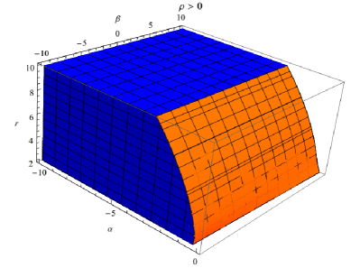
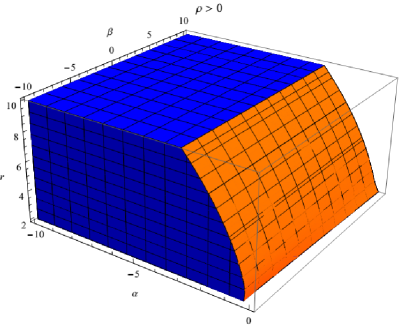
Figure 1: The evolution of $\rho$ w.r.t. $r$, with the left side representing $\lambda>0$ and the right side representing $\lambda<0$.

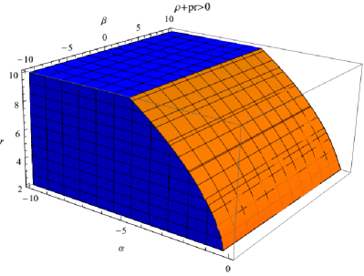
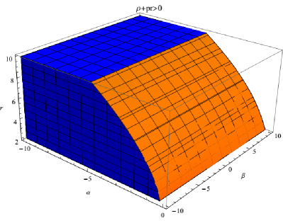
Figure 2: The evolution of $\rho+P_{r}$ w.r.t. $r$, with the left side representing $\lambda>0$ and the right side representing $\lambda<0$.

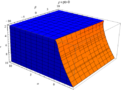
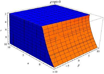
Figure 3: The evolution of $\rho+P_{t}$ w.r.t. $r$, with the left side representing $\lambda>0$ and the right side representing $\lambda<0$.

While, the behavior od $\rho$, $P_{r}$ and $P_{t}$ are shown in in fig. (4).

Figure 4: The behaviour of $\rho(r),P_{r}(r)$ and $P_{t}(r)$ w.r.t. $r$.

2.1.1 A State of Equilibrium

Here, we evaluate the classification of WH-models in the equilibrium state. One can find equilibrium state for WH by solving the Tolman-Oppenheimer-Volkov (TOV) equation, given as,

$$\frac{{d{P_{r}}}}{{dr}}+\frac{2}{r}\left(\rho-{P_{r}}\right)+a^{\prime}\left(\rho+{P_{r}}\right)+\frac{\lambda}{3(1+\lambda)}\frac{d}{dr}(3\rho+P_{r}-2P_{t})=0.$$ (18)

The above expression (18) shows that the gravitational ($F_{gf}$), the hydrostatic ($~{}F_{hf}$), the extra (matter-coupling) force ($F_{ext}$) and, the anisotropic ($F_{af}$) are the major forces here. The mathematical expressions of these forces are as follows:

$${F_{gf}}=-\frac{1}{2}{\sigma^{\prime}[\sigma+{P_{r}}]},~{}~{}{F_{hf}}=-\frac{{d{P_{r}}}}{{dr}},~{}~{}{F_{af}}=\frac{{2\Pi}}{r},F_{ext}=\frac{\lambda}{3(1+\lambda)}\frac{d}{dr}(3\rho+P_{r}-2P_{t})$$

where $\sigma=2a(r)$. Keeping in view the above expressions of forces, the Eq.(18) may be reduced to the following,

$${F_{gf}}+{F_{hf}}+{F_{af}}+F_{ext}=0.$$ (19)

The behavior for these forces can be shown in Fig. (5), in which we see that the $F_{g}$ and $F_{ext}$ are almost negligible while the reaming two forces cancel the effects of each others.

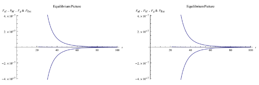
Figure 5: The behaviour of different forces, with the left side representing $\lambda>0$ and the right side representing $\lambda<0$.

2.2 Isotropic Matter Distribution

In our case, we assume the coupling of a perfect matter distribution with WH geometry. Researchers in the field of relativistic astrophysics have used isotropic matter distributions to look at a number of important problems in astrophysics. Some of these problems are the gravitational collapse rate, the stability analysis of astronomical systems, the system’s energy density irregularities, the universe’s stable configurations maintenance and many others. In our case, we have a system that allows for equal pressure components ($P_{r}=P_{t}=P$ or $\Pi=0$). Given the circumstances, the solutions to equations for $P_{r}$ and $P_{t}$ combine to form a non-linear third-order differential equation. Now, if we solve this equation again by incorporating $\beta(r)$ and $b(r)$, we get a third-order non-linear differential equation. We cannot use analytical methods to solve this updated third-order non-linear differential equation, so we use different numerical methods to solve it.
Along with the numerical techniques, we implement some initial and boundary conditions for solving this updated differential equation. The boundary conditions used are: $\beta(r_{0})=03$, ${\beta^{\prime}}(r_{0})=0$ and $\beta(10)=1$. Finally, we plot different solutions to this equation to check the role of NEC and WEC, as shown in Fig. (6)-(8).

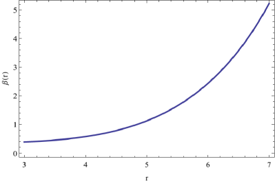
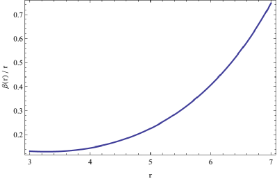
Figure 6: The evolution of $\beta(r)$ and $\beta(r)/r$ w.r.t. $r$ for isotropic matter distribution.

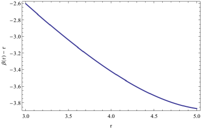
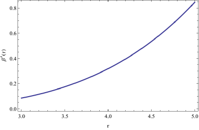
Figure 7: The evolution of $\beta(r)-r$ and $\beta^{\prime}(r)$ w.r.t. $r$ for isotropic matter distribution.

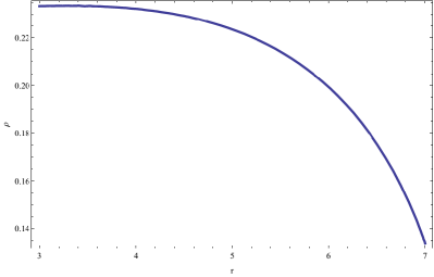
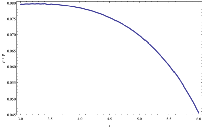
Figure 8: The evolution of $\rho(r)$ and $\rho+P$ w.r.t. $r$ for isotropic matter distribution.

2.3 Barotropic EoS

Here, we demonstrate the relationship between $\rho$ and $P$ using a well-established cosmological-EoS and a dimensionless parameter ($k$). The realistic modeling of the barotropic-EoS results in the representations: $P_{r}=k\rho$ or $P_{r}-k\rho=0$. It is possible to broaden the scope of this study using equivalent $P_{t}$ with $\rho$ and EoS parameters (say $n$) as: $P_{t}=n\rho$ [94]. In this case, we use the value of $P_{r}$ and $\rho$ along with transform $b(r)$ to $\beta(r)$ to get a third-order nonlinear differential equation. We then use numerical methods to draw different plots of $\beta(r)$ that are illustrated in Fig.9. In the Fig.9, left plot illustrates an increasing distribution of $\beta(r)$ for barotropic-EoS and that apparently WH throat lies at $r_{0}=3$ where $\beta(3)=3$. The right plot of the Fig.9 shows that $1>\beta^{\prime}(r_{0})$. The flare-out and asymptotic limits can be investigated using the plots ($\frac{\beta(r)}{r}$ and $\beta(r)-r$) shown in Fig.10. The left plot of the Fig.10 shows that the condition $\frac{\beta(r)}{r}\rightarrow 0$ is not valid in the range $r\rightarrow\infty$ . While the right plot of the Fig.10 shows that the flare-out limit is applicable. The Fig.11 shows that the WEC is not satisfied while the NEC is fulfilled. As a result, no feasible WH configurations are located in this specific region.

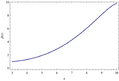
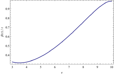
Figure 9: The evolution of $\beta(r)$ and $\beta(r)/r$ w.r.t. $r$ for barotropic EoS.

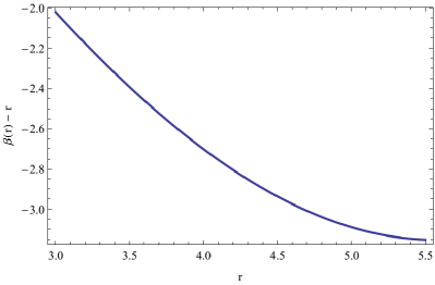
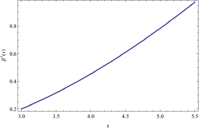
Figure 10: The evolution of $\beta(r)-r$ and $\beta^{\prime}(r)$ w.r.t. $r$ for barotropic EoS.

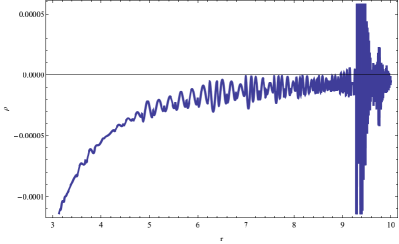
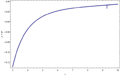
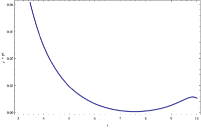
Figure 11: The evolution of $\rho(r)$, $\rho+P_{r}$ and $\rho+P_{t}$ w.r.t. $r$ for barotropic EoS.

3 Conclusions

Previous research establishes that for an ideal and viable WH-model, a mandatory component is required. This component must obey a certain limit of violations of the ECs in a given feasible system. Nonetheless, considering the MGTs framework obtains the outcome of $T_{\sigma\lambda}^{\textit{effective}}$ fulfils ECs while passes through WH throat. Furthermore, the additional curvature corrections support the extraordinary WH geometries. We used $f(R,G,T)$-MGT framework for obtaining static spherically symmetric WH solutions, that couples with isotropic, anisotropic, and barotropic EoS. We investigated the impact of $f(R,G,T)$-MGT on WH models by investigating the role of various ECs (WEC, NEC) with different matter distributions (perfect, anisotropic, and barotropic fluids). Many designated methods are proposed in the literature for describing WH models. Various schemes are used in these methods, such as considering the $\beta(r)$ for WH and then investigating ECs, selecting appropriate fluid mechanisms and then computing $\beta(r)$. Our investigations in this paper are limited to the framework of $f(R,G,T)$-MGT, which includes matter couplings with Ricci variables. We used the following model to examine the viability of WH solutions: $f(R,G,T)=R+\alpha R^{2}+\beta G^{n}+\gamma G\ln(G)+\lambda T$. Our calculations are very tedious and involve comparatively complicated nonlinear differential equations with unknown functions ($\rho,P_{r},P_{t},a,b,f(R,G,T)$), so some unique factors play a crucial role in these calculations.
Considering our findings, we report that the violation of NEC by matter passing through the WH throat can be validated using the stress energy tensor. Next to this, we briefly studied solutions of the gravitational FEqs using different matter distributions (isotropic, anisotropic, and barotropic fluids). We studied these equations using $\beta(r)$ with quadratic Ricci scalar function and assuming $f(T)=\lambda T$. In the case of isotropic and barotropic matter distributions, the nonlinear differential equations are computed using numerical methods and the corresponding results are presented by plotting $\beta(r)$. Our plots locate some regions in which WH fulfills the ECs. Moreover, we analyzed the significance of the equilibrium state and obtained that $F_{hf}$ and $F_{gf}$ balance each other.
To obtain viable WH solutions in $f(R,G,T)$-MGT, a specific model is considered, and then FEqs are determined using a set of $\beta(r)$. The behaviour of ECs (NEC, WEC) is examined by plotting different regions corresponding to a set of values of $r,\alpha$ and $\beta$. Resultantly, we obtained some regions for viable WHs in the absence of exotic matter. We also examined the equilibrium state for anisotropic matter distribution using these plots and found that $F_{hf}$ and $F_{af}$ cancel the effect of each other while the $F_{g}$ and $F_{ext}$ are almost negligible. These plots shows the numerical results for $\beta(r)$ in the background of barotropic EoS.

Author Contributions:

M.I, A.R.A., F.K., N.G., H.I.A., K.S.N., A.-H.A.-A. have contributed equally. All authors have read and agreed to the published version of the manuscript.

Funding:

This work was supported by Princess Nourah bint Abdulrahman University Researchers Supporting Project number (PNURSP2023R106), Princess Nourah bint Abdulrahman University, Riyadh, Saudi Arabia.

Data availability statement

All data generated or analyzed during this study are included in this published article.

Conflicts of Interest:

The authors declare no conflict of interest.

References

- [1] Saul Perlmutter, Goldhaber Aldering, Gerson Goldhaber, RA Knop, Peter Nugent, Patricia G Castro, Susana Deustua, Sebastien Fabbro, Ariel Goobar, Donald E Groom, et al. Measurements of and from 42 high-redshift supernovae. The Astrophysical Journal, 517(2):565, 1999.
- [2] Adam G Riess, Alexei V Filippenko, Peter Challis, Alejandro Clocchiatti, Alan Diercks, Peter M Garnavich, Ron L Gilliland, Craig J Hogan, Saurabh Jha, Robert P Kirshner, et al. Observational evidence from supernovae for an accelerating universe and a cosmological constant. The Astronomical Journal, 116(3):1009, 1998.
- [3] PAR Ade, N Aghanim, Z Ahmed, RW Aikin, KD Alexander, M Arnaud, et al. Bicep2 and planck collaborations. Phys. Rev. Lett, 114(10):101301, 2015.
- [4] BICEP Collaborations, PAR Ade, Z Ahmed, RW Aikin, KD Alexander, D Barkats, SJ Benton, CA Bischoff, JJ Bock, R Bowens-Rubin, et al. Improved constraints on cosmology and foregrounds from bicep2 and keck array cosmic microwave background data with inclusion of 95 ghz band. Physical Review Letters, 116(3):031302, 2016.
- [5] Max Tegmark, Michael A Strauss, Michael R Blanton, Kevork Abazajian, Scott Dodelson, Havard Sandvik, Xiaomin Wang, David H Weinberg, Idit Zehavi, Neta A Bahcall, et al. Cosmological parameters from sdss and wmap. Physical review D, 69(10):103501, 2004.
- [6] Uroš Seljak, Alexey Makarov, Patrick McDonald, Scott F Anderson, Neta A Bahcall, J Brinkmann, Scott Burles, Renyue Cen, Mamoru Doi, James E Gunn, et al. Cosmological parameter analysis including sdss ly forest and galaxy bias: constraints on the primordial spectrum of fluctuations, neutrino mass, and dark energy. Physical Review D, 71(10):103515, 2005.
- [7] Daniel J Eisenstein, Idit Zehavi, David W Hogg, Roman Scoccimarro, Michael R Blanton, Robert C Nichol, Ryan Scranton, Hee-Jong Seo, Max Tegmark, Zheng Zheng, et al. Detection of the baryon acoustic peak in the large-scale correlation function of sdss luminous red galaxies. The Astrophysical Journal, 633(2):560, 2005.
- [8] Bhuvnesh Jain and Andy Taylor. Cross-correlation tomography: measuring dark energy evolution with weak lensing. Physical Review Letters, 91(14):141302, 2003.
- [9] M Ilyas, AR Athar, and Bilal Masud. Relativistic charged sphere in gravity. International Journal of Geometric Methods in Modern Physics, 18(10):2150152, 2021.
- [10] M Ilyas and AR Athar. Some specific wormhole solutions in gravity. Physica Scripta, 97(4):045003, 2022.
- [11] M Ilyas, AR Athar, Z Yousaf, Bilal Masud, and Fawad Khan. The bouncing behavior in gravity. Indian Journal of Physics, pages 1–11, 2022.
- [12] M Ilyas, WU Rahman, S Ullah, F Khan, H Ullah, and R Khan. Wormhole solutions through hyperbolic model in gravity. International Journal of Modern Physics D, 31(05):2250034, 2022.
- [13] M Ilyas. Charged compact stars in gravity. The European Physical Journal C, 78(9):757, 2018.
- [14] S Nojiri and SD Odintsov. Introduction to modified gravity and gravitational alternative for dark energy. arXiv preprint hep-th/0601213, 2006.
- [15] Thomas P Sotiriou and Valerio Faraoni. theories of gravity. Reviews of Modern Physics, 82(1):451, 2010.
- [16] Shin’ichi Nojiri and Sergei D Odintsov. Unified cosmic history in modified gravity: from f (R) theory to lorentz non-invariant models. Physics Reports, 505(2-4):59–144, 2011.
- [17] Salvatore Capozziello and Mariafelicia De Laurentis. Extended theories of gravity. Physics Reports, 509(4-5):167–321, 2011.
- [18] V Faraoni and S Capozziello. The landscape beyond einstein gravity. Beyond Einstein Gravity, 170:59–106, 2010.
- [19] Kazuharu Bamba, Salvatore Capozziello, Shin’ichi Nojiri, and Sergei D Odintsov. Dark energy cosmology: the equivalent description via different theoretical models and cosmography tests. Astrophysics and Space Science, 342(1):155–228, 2012.
- [20] De la Cruz-Dombriz, Diego Sáez-Gómez, et al. Black holes, cosmological solutions, future singularities, and their thermodynamical properties in modified gravity theories. Entropy, 14(9):1717–1770, 2012.
- [21] Austin Joyce, Bhuvnesh Jain, Justin Khoury, and Mark Trodden. Beyond the cosmological standard model. Physics Reports, 568:1–98, 2015.
- [22] Kazuya Koyama. Cosmological tests of modified gravity. arXiv preprint arXiv:1504.04623, 2015.
- [23] Kazuharu Bamba, Shin’ichi Nojiri, and Sergei D Odintsov. Modified gravity: walk through accelerating cosmology. arXiv preprint arXiv:1302.4831, 2013.
- [24] Kazuharu Bamba and Sergei D Odintsov. Universe acceleration in modified gravities: and cases. arXiv preprint arXiv:1402.7114, 2014.
- [25] Kazuharu Bamba and Sergei D Odintsov. Inflationary cosmology in modified gravity theories. Symmetry, 7(1):220–240, 2015.
- [26] M Sharif and Z Yousaf. Role of adiabatic index on the evolution of spherical gravitational collapse in palatini gravity. Astrophysics and Space Science, 355(2):317–331, 2015.
- [27] Z Yousaf, M Bhatti, and Ume Farwa. Stability of compact stars in r 2+ (r t ) gravity. Monthly Notices of the Royal Astronomical Society, 464(4):4509–4519, 2017.
- [28] Tiberiu Harko, Francisco SN Lobo, Shin’ichi Nojiri, and Sergei D Odintsov. gravity. Physical Review D, 84(2):024020, 2011.
- [29] MJS Houndjo. Reconstruction of gravity describing matter dominated and accelerated phases. International Journal of Modern Physics D, 21(01):1250003, 2012.
- [30] M Sharif and Z Yousaf. Energy density inhomogeneities in charged radiating stars with generalized CDTT model. Astrophysics and Space Science, 354(2):431–441, 2014.
- [31] M Sharif and Z Yousaf. Radiating cylindrical gravitational collapse with structure scalars in gravity. Astrophysics and Space Science, 357(1):1–11, 2015.
- [32] B Mishra. Sankarsan tarai, sk tripathy, adv. high. Energy Phys, 8543560(1), 2016.
- [33] PK Sahoo, A Nath, and SK Sahu. Bianchi type-iii string cosmological model with bulk viscous fluid in lyra geometry. Iranian Journal of Science and Technology, Transactions A: Science, 41(1):243–248, 2017.
- [34] Hamid Shabani and Amir Hadi Ziaie. Stability of the einstein static universe in gravity. Eur. Phys. J. C, 77:31, 2017.
- [35] Ch C Moustakidis. The stability of relativistic stars and the role of the adiabatic index. General Relativity and Gravitation, 49(5):68, 2017.
- [36] Z Yousaf, M Zaeem-ul Haq Bhatti, and Aamna Rafaqat. LTB geometry with tilted and nontilted congruences in gravity. International Journal of Modern Physics D, 26(09):1750099, 2017.
- [37] M Ilyas. Compact stars in gravity. International Journal of Modern Physics A, 36(24):2150165, 2021.
- [38] M Ilyas, Aftab Ahmad, Fawad Khan, and M Wasif. Energy conditions in extended gravity. Physica Scripta, 98(1):015016, 2022.
- [39] M Ilyas, AR Athar, and Asma Bibi. Charged compact stars in extended gravity. New Astronomy, page 102053, 2023.
- [40] Homer G Ellis. Ether flow through a drainhole: A particle model in general relativity. Journal of Mathematical Physics, 14(1):104–118, 1973.
- [41] KA Bronnikov. Scalar-tensor theory and scalar charge. Acta Physica Polonica. Series B, 4(2):251–266, 1973.
- [42] Gerard Clement. Einstein-yang-mills-higgs solitons. General Relativity and Gravitation, 13(8):763–770, 1981.
- [43] Michael S Morris and Kip S Thorne. Wormholes in spacetime and their use for interstellar travel: A tool for teaching general relativity. American Journal of Physics, 56(5):395–412, 1988.
- [44] Matt Visser. Lorentzian wormholes. from einstein to hawking. Woodbury, 1995.
- [45] David Hochberg and Matt Visser. Dynamic wormholes, antitrapped surfaces, and energy conditions. Physical Review D, 58(4):044021, 1998.
- [46] Peter KF Kuhfittig. Wormholes supported by a combination of normal and quintessential matter in Einstein and Einstein-Maxwell gravity. arXiv preprint arXiv:1212.0153, 2012.
- [47] RA Konoplya and A Zhidenko. Traversable wormholes in general relativity without exotic matter. arXiv preprint arXiv:2106.05034, 2021.
- [48] Francisco SN Lobo. Exotic solutions in general relativity: Traversable wormholes and ’warp drive’spacetimes. arXiv preprint arXiv:0710.4474, 2007.
- [49] Peter KF Kuhfittig. More on wormholes supported by small amounts of exotic matter. Physical Review D, 73(8):084014, 2006.
- [50] Francisco SN Lobo. Wormhole geometries in modified gravity. In AIP Conference Proceedings, volume 1458, pages 447–450. American Institute of Physics, 2012.
- [51] PHRS Moraes and PK Sahoo. Nonexotic matter wormholes in a trace of the energy-momentum tensor squared gravity. Physical Review D, 97(2):024007, 2018.
- [52] PK Sahoo, PHRS Moraes, Parbati Sahoo, and G Ribeiro. Phantom fluid supporting traversable wormholes in alternative gravity with extra material terms. International Journal of Modern Physics D, 27(16):1950004, 2018.
- [53] Nisha Godani and Gauranga C Samanta. Static traversable wormholes in gravity. Chinese Journal of Physics, 62:161–171, 2019.
- [54] Nisha Godani and Gauranga C Samanta. Wormhole modeling in gravity with linear trace term. International Journal of Modern Physics A, 35(08):2050045, 2020.
- [55] Parbati Sahoo, Sanjay Mandal, and PK Sahoo. Wormhole model with a hybrid shape function in gravity. New Astronomy, 80:101421, 2020.
- [56] Parbati Sahoo, PHRS Moraes, Marcelo M Lapola, and PK Sahoo. Traversable wormholes in the traceless gravity. International Journal of Modern Physics D, 30(13):2150100, 2021.
- [57] Eloy Ayón-Beato, Fabrizio Canfora, and Jorge Zanelli. Analytic self-gravitating skyrmions, cosmological bounces and ads wormholes. Physics Letters B, 752:201–205, 2016.
- [58] Fabrizio Canfora, Nikolaos Dimakis, and Andronikos Paliathanasis. Topologically nontrivial configurations in the 4d einstein-nonlinear -model system. Physical Review D, 96(2):025021, 2017.
- [59] Carlos Barcelo and Matt Visser. Traversable wormholes from massless conformally coupled scalar fields. Physics Letters B, 466(2-4):127–134, 1999.
- [60] Cosimo Bambi, Alejandro Cardenas-Avendano, Gonzalo J Olmo, and D Rubiera-Garcia. Wormholes and nonsingular spacetimes in palatini gravity. Physical Review D, 93(6):064016, 2016.
- [61] S Nojiri, O Obregon, SD Odintsov, and KE Osetrin. Induced wormholes due to quantum effects of spherically reduced matter in large n approximation. Physics Letters B, 449(3-4):173–179, 1999.
- [62] S Nojiri, O Obregon, SD Odintsov, and KE Osetrin. Can primordial wormholes be induced by GUTs at the early universe. Physics Letters B, 458(1):19–28, 1999.
- [63] SV Sushkov. A selfconsistent semiclassical solution with a throat in the theory of gravity. Physics Letters A, 164(1):33–37, 1992.
- [64] Remo Garattini and Francisco SN Lobo. Self-sustained phantom wormholes in semi-classical gravity. Classical and Quantum Gravity, 24(9):2401, 2007.
- [65] Luis A Anchordoqui and Santiago E Perez Bergliaffa. Wormhole surgery and cosmology on the brane: The world is not enough. Physical Review D, 62(6):067502, 2000.
- [66] KA Bronnikov and Sung-Won Kim. Possible wormholes in a brane world. Physical Review D, 67(6):064027, 2003.
- [67] ErnestoF Eiroa and Griselda Figueroa Aguirre. Thin-shell wormholes with a generalized chaplygin gas in einstein–born–infeld theory. The European Physical Journal C, 72(11):2240, 2012.
- [68] Ernesto F Eiroa and Claudio Simeone. Stability of chaplygin gas thin-shell wormholes. Physical Review D, 76(2):024021, 2007.
- [69] M Sharif and Z Yousaf. Cylindrical thin-shell wormholes in gravity. Astrophysics and Space Science, 351(1):351–360, 2014.
- [70] Francisco SN Lobo. Chaplygin traversable wormholes. Physical Review D, 73(6):064028, 2006.
- [71] Martin G Richarte and Claudio Simeone. Thin-shell wormholes supported by ordinary matter in einstein-gauss-bonnet gravity. Physical Review D, 76(8):087502, 2007.
- [72] Panagiota Kanti, Burkhard Kleihaus, and Jutta Kunz. Wormholes in dilatonic einstein-gauss-bonnet theory. Physical review letters, 107(27):271101, 2011.
- [73] Christian G Boehmer, Tiberiu Harko, and Francisco SN Lobo. Wormhole geometries in modified teleparallel gravity and the energy conditions. Physical Review D, 85(4):044033, 2012.
- [74] Sayan Kar. Evolving wormholes and the weak energy condition. Physical Review D, 49(2):862, 1994.
- [75] Arkadii A Popov. Stress-energy of a quantized scalar field in static wormhole spacetimes. Physical Review D, 64(10):104005, 2001.
- [76] C Armendariz-Picon. On a class of stable, traversable lorentzian wormholes in classical general relativity. Physical Review D, 65(10):104010, 2002.
- [77] Hideki Maeda and Masato Nozawa. Static and symmetric wormholes respecting energy conditions in einstein-gauss-bonnet gravity. Physical Review D, 78(2):024005, 2008.
- [78] Francisco SN Lobo and Miguel A Oliveira. Wormhole geometries in modified theories of gravity. Physical Review D, 80(10):104012, 2009.
- [79] Nadiezhda Montelongo Garcia and Francisco SN Lobo. Nonminimal curvature–matter coupled wormholes with matter satisfying the null energy condition. Classical and Quantum Gravity, 28(8):085018, 2011.
- [80] M Hamani Daouda, MJS Houndjo, and Manuel E Rodrigues. New static solutions in theory. Eur. Phys. J. C, 71(arXiv: 1108.2920):1817, 2011.
- [81] Christian G Boehmer, Tiberiu Harko, and Francisco SN Lobo. Wormhole geometries in modified teleparallel gravity and the energy conditions. Physical Review D, 85(4):044033, 2012.
- [82] Mubasher Jamil, Davood Momeni, and Ratbay Myrzakulov. Wormholes in a viable gravity. European Physical Journal C, 73:2267, 2013.
- [83] Z Yousaf, M Ilyas, and M Zaeem-ul-Haq Bhatti. Static spherical wormhole models in gravity. The European Physical Journal Plus, 132(6):1–12, 2017.
- [84] Z Yousaf, M Ilyas, and MZ Bhatti. Influence of modification of gravity on spherical wormhole models. Modern Physics Letters A, 32(30):1750163, 2017.
- [85] MZ Bhatti, Z Yousaf, and M Ilyas. Existence of wormhole solutions and energy conditions in gravity. Journal of Astrophysics and Astronomy, 39(6):1–11, 2018.
- [86] Z Yousaf, A Ikram, M Ilyas, and MZ Bhatti. Existence of dynamical wormholes in gravity. Canadian Journal of Physics, 98(5):474–483, 2020.
- [87] Tiberiu Harko and Francisco SN Lobo. Generalized curvature-matter couplings in modified gravity. Galaxies, 2(3):410–465, 2014.
- [88] Orfeu Bertolami, Francisco SN Lobo, and Jorge Páramos. Nonminimal coupling of perfect fluids to curvature. Physical Review D, 78(6):064036, 2008.
- [89] Tahereh Azizi. Wormhole geometries in gravity. International Journal of Theoretical Physics, 52(10):3486–3493, 2013.
- [90] PHRS Moraes and PK Sahoo. Modeling wormholes in gravity. Physical Review D, 96(4):044038, 2017.
- [91] Eric Poisson. A relativist’s toolkit: the mathematics of black-hole mechanics. Cambridge university press, 2004.
- [92] Naresh Dadhich. Derivation of the raychaudhuri equation. arXiv preprint gr-qc/0511123, 2005.
- [93] M Ilyas. Energy conditions in non-local gravity. International Journal of Geometric Methods in Modern Physics, 16(10):1950149, 2019.
- [94] PHRS Moraes and PK Sahoo. Nonexotic matter wormholes in a trace of the energy-momentum tensor squared gravity. Physical Review D, 97(2):024007, 2018.