On the effectiveness of null TDI channels as instrument noise monitors in LISA

Abstract

We present a study of the use and limits of the Time-Delay Interferometry null channels for in flight estimation of the Laser Interferometer Space Antenna instrumental noise. The paper considers how the two main limiting noise sources, test-mass acceleration noise and interferometric phase measurement noise, propagate through different Time-Delay Interferometry channels: the Michelson combination X that is the most sensitive to gravitational waves, then the less-sensitive combinations $\alpha$, and finally the null channel $\zeta$. We note that the null channel $\zeta$, which is known to be equivalent to any null channel, not only has a reduced sensitivity to the gravitational waves, but also feature a larger degree of cancellation of the test mass acceleration noise relative to the interferometry noise. This severely limits its use in quantifying the low frequency instrumental noise in the Michelson X combination, which is expected to be dominated by acceleration noise. However, we show that one can still use in-flight noise estimations from $\zeta$ to put an upper bound on the considered noises entering in the X channel, which allows to distinguish them from a strong stochastic gravitational wave background.

I Introduction

The Laser Interferometer Space Antenna (LISA) gravitational wave observatory Amaro-Seoane et al. (2017) is expected to be continuously dominated by gravitational wave (GW) signals in its $\mathrm{mHz}$ frequency band. This implies a technical difficulty in quantifying and understanding the instrumental noise of LISA in the constant presence of GW signals, which is essential for maximizing the observatory scientific return and to identify possible Stochastic Gravitational Wave Backgrounds (SGWBs) Amaro-Seoane et al. (2017). The LISA scientific observables are constructed from so-called Time-Delay Interferometry (TDI) combinations, which synthesize equal arm interferometers to cancel an otherwise overwhelming contribution from laser frequency noise Armstrong et al. (1999). The primary GW observables will be obtained from TDI channels such as the Michelson X channel. This channel represents a virtual interferometer with the same principle of measurements of a standard Michelson interferometer, as they are used in ground based GW observatories, such as LIGO, Virgo and Kagra.

In addition to these sensitive channels, it has been shown that so-called null channels can be constructed, which strongly suppress the GW signals at low frequencies and might therefore be used for characterizing the instrumental noise Armstrong et al. (1999); Hogan and Bender (2001a); Muratore et al. (2022). An example is the null channel $\zeta$, which represents a symmetric measurement across all three arms of the constellation, strongly suppressing its response to GWs at low frequencies Muratore et al. (2020). It is shown in Muratore et al. (2022) that all possible null channels can be derived from the $\zeta$ channel. Thus, it is sufficient to exclusively focus on $\zeta$ to study the relationship between TDI channels sensitive to GWs and null channels. The results obtained are then generally applicable to any null channel.

We notice that, compared to ground-based GW obseratories, a null channel is particularly valuable in LISA. While ground-based observatories can exploit correlations between multiple detectors to discriminate the GWs from instrumental noise sources, LISA will be a single detector, such that the same kind of analysis might not be possible. Furthermore, as mentioned above, LISA is expected to be signal dominated, such that instrumental noise cannot be measured and characterized in flight in isolation from the GW signals.
Current approaches to the data analysis for LISA foresee a ”global fit”, in which an initial noise model will be defined to start subtracting resolvable sources in an iterative procedure Littenberg and Cornish (2023). While the background residual noise model is refined in this iterative process, improving the identification of the known sources, the residual noise model does not necessarily distinguish between instrumental and gravitational noise. As our a priori knowledge of the instrumental noise background is likely to have limited accuracy, this poses a fundamental problem in the identification of a stochastic GW background. The goal of this paper is to analyze the extent to which the null channel can be used to characterize the dominant noise sources expected to affect the sensitive channels. We then further explore what this implies for the detectability of an isotropic SGWB of unknown spectral shape.

Following the LISA proposal Amaro-Seoane et al. (2017), we consider two general groups of instrumental noise sources: the test mass (TM) acceleration noise and the effective total displacement noise in a one-way single link TM to TM measurement, which we abbreviate as Optical Metrology System (OMS) noise. As we will discuss in section II, each of these two groups of noise in reality represents a multitude of individual noise contributions driven by different physical effects, both known and possible unknown, such that the exact level and frequency dependence of these LISA instrumental noises cannot be reliably calculated a priori. As an example of the difficulty in accurately modeling noise a priori, the acceleration noise at $0.1\text{\,}\mathrm{mHz}$ measured by LISA Pathfinder (LPF), though compatible with the LISA noise requirements, exceeds by approximately a factor 4 the noise accounted for by the noise model Armano et al. (2018). Various key parameters of the LISA noise, including DC residual forces Armano et al. (2016), magnetic field gradients Armano et al. (2020), residual stray electrostatic fields Antonucci et al. (2012), optical alignments Chwalla et al. (2020); Hartig et al. (2022), among others, are all designed to be ideally zero, but with uncertainties that make their residual contribution to the observatory noise both difficult to predict and likely different among the different LISA TM or optical readouts. Other well known noise sources like Brownian noise from gas damping can have a non-trivial time dependence and thus an instantaneous noise Power Spectral Density (PSD) that is hard to predict Armano et al. (2017). As such, if noise knowledge is a key factor in extracting LISA science, either for a stochastic background or for noise priors on individual source parameters, then developing in situ techniques to quantify the instrument noise is an important task.

TM acceleration noise is expected to limit the GW sensitive channels, such as the Michelson X, at low frequencies (below a few $\mathrm{mHz}$), while the OMS noise is most relevant for the sensitivity of these channels at high frequencies. On the contrary, we will show that TM acceleration noise is effectively suppressed in the $\zeta$ channel, such that it is dominated by OMS noise at all frequencies. This behaviour of the null channels has already been pointed out in Flauger et al. (2021); Wang et al. (2022) for the null channel T that is built out of X and the two channels Y and Z (obtained from X by cyclic satellite permutations), considering the case of LISA with equal arm-lengths. However, as already shown in Adams and Cornish (2010) and Muratore et al. (2022), T as a null channel is strongly compromised when the arm lengths are not exactly equal, especially at low frequencies. The null channel $\zeta$ remains less sensitive to GW also in the more general unequal arm-lengths scenario. Therefore in the rest of the paper we will discuss only the properties of $\zeta$, and we will simplify the formulas presented to the equal armlength approximation, which has negligable impact on the general conclusions. We will re-introduce the inequality of the arm-lengths when necessary to not bias the computations, and also perform time-domain simulations using realistic orbits to show our equal-armlength models are accurate enough. We discuss in sections III and IV the impact of our findings, showing that the dominant OMS noise in the null channel strongly limits its effectiveness for noise characterization in the low frequency regime. For instance, for a null channel measurement to detect the TM acceleration noise relevant to the Michelson X combination at $0.1\text{\,}\mathrm{mHz}$, the OMS noise would have to be at the $0.1\text{\,}\mathrm{n}\mathrm{m}\mathrm{/}\sqrt{\mathrm{Hz}}$ level at $0.1\text{\,}\mathrm{mHz}$ compared to the requirement of $6\text{\,}\mathrm{n}\mathrm{m}\mathrm{/}\sqrt{\mathrm{Hz}}$ defined in the proposal Amaro-Seoane et al. (2017), as shown in fig. 3. Such a low noise level is neither foreseen nor required for LISA GW observation in the TDI Michelson X, Y and Z channels (or the equivalent orthogonal combinations of these, A and E Prince et al. (2002)). Given the inherent uncertainties in the modelling of the noise sources composing the LISA full noise budget pre-flight, we conclude that the null channels can only yield very weak upper limits on the low frequency TM acceleration noise. These constraints on the noise in X become more stringent towards higher frequencies, where both X and $\zeta$ are dominated by OMS noise (assuming nominal performance). Note that at very high frequencies, $\zeta$ becomes equally sensitive to X, such that the frequency band in which we can put strong constraints on the instrumental noise in X is rather limited.

The remaining article is divided in four main sections. In section II, we introduce the noise models defined in the LISA proposal and discuss in detail the TDI outputs. In section III we discuss the use of these null channels to calibrate and measure the instrumental noise during operations and the implication for distinguishing between instrumental noise and SGWB. In section IV, we compare our analytical calculations with time domain simulations using the tools LISA Instrument, LISA GW-Response and PyTDI, which we configured to reflect the noise models given in the LISA proposal Bayle and Hartwig (2020) and our semi-analytical GW response computation. We also study the response of the significantly less sensitive (compared to X) Sagnac channel $\alpha$, and we explore to which extent the noise entering in $\alpha$ could be combined with the null channel $\zeta$. Finally, we use $\zeta$ to compute an upper limit on the instrumental noise in X, which allows us to identify a strong SGWB in the X data stream.

In the last section we report our conclusion and future perspective.

II Instrumental noise modeling and TDI outputs

In this section, we briefly introduce the main limiting noise sources left after TDI suppression of laser frequency noise, and any possible further subtraction of any known calibrated and measured instrumental noise sources, such as, for example, the optical tilt to length cross-coupling to spacecraft motion (Hartig et al. (2022) and Chwalla et al. (2020)).

The remaining noises, for which we have neither a measurement for coherent subtraction nor a high precision a priori model, falls into two broad categories Amaro-Seoane et al. (2017), the acceleration noise of each individual TM and an overall optical metrology noise term for each single link measurement. For the GW sensitive TDI channels, the former is expected to be the limiting noise source at low frequencies, while the latter is most relevant at high frequencies. We then compute how these noise sources propagate through different TDI channels, and discuss to which extent and at which frequencies the null channel can be a useful noise monitor for the GW sensitive channels.

We will express the phase outputs measured by LISA, used to build the TDI channels, as an effective displacement signal in units of meters.

II.1 TM acceleration noise

In the assumption of a perfect spacecraft jitter subtraction, we can ignore the complications of the split interferometry scheme Amaro-Seoane et al. (2017) and assume for the calculation of the TDI outputs that the two optical-benches, say $\mathrm{OB}_{i}$ and $\mathrm{OB}_{j}$, were two free-falling particles that accelerate along their relative line of sight towards each other with accelerations $g_{i}$ and $g_{j}$ respectively. $g_{i}$ and $g_{j}$ describe the TMs acceleration noise with respect to the local inertial frame, that for LISA, can be associated with the one defined by the incoming laser beam (See appendix B).

We will denote the overall TM acceleration noise PSD of a single TM as $S_{g_{ij}}$. We assume for simplicity that all TM acceleration noises are fully uncorrelated to each other, although this might not be the case in reality. Furthermore, in our assumptions of free-falling optical benches, we can directly convert the acceleration noise of a single TM to an equivalent displacement of the correspondent optical bench, whose PSD is given as

$$S_{g_{ij}}^{disp}=S_{g_{ij}}/(2\pi f)^{4}.$$ (1)

We will denote the time series associated with this displacement as $x^{g}_{ij}(t)$.

Note that the exact noise shape and amplitude of each individual $S_{g_{ij}}$ will result from the superposition of a multitude of physical effects. While many of these effects have been characterized during the very successful LPF mission, the total measured noise is considerably larger than the sum of these known sources, indicating the difficulty in achieving a complete, accurate model Armano et al. (2018, 2022). We therefore cannot assume to have accurate prior knowledge of the overall acceleration noise, and would need to rely on in-flight measurements to constrain its value for each TM.

II.2 Optical Metrology System noise

We summarize as OMS noise any imperfection in the ability of the OMS to determine the separation between two TMs in a single link.
Similar to the overall acceleration noise acting on each TM, the overall OMS noise affecting a single link will be a superposition of many physical effects. In addition, the overall OMS noise summarizes noise entering due to different instrumental subsystems, such as the telescope, optical bench, phase measurement system, laser, clock and TDI processing Amaro-Seoane et al. (2017). Note that some of these noise sources can again be correlated (similar to the TM acceleration noise), while here we assume they are not.

For simplicity, we consider only a single uncorrelated noise term in each single link measurement, whose PSD we denote by $S_{oms_{ij}}(f)$. We will denote the time series of these single link OMS as $x^{m}_{ij}(t)$.

We remark that while the TM acceleration was measured by LPF in realistic flight conditions, we expect new challenges and additional uncertainty in the pre-flight characterization of the OMS. While many terms in the OMS budget are well calculated from models and ground testing (such as shot noise and phasemeter noise), the end-to-end inter-spacecraft LISA optical measurement has never been performed and we can expect unknowns. This is especially true for the low frequency regime, as there will likely be no possible on-ground long term testing before flight ($>$ 1 month). We also cannot assume this noise to be stationary over the mission duration, as we must expect that some of the physical parameters governing its level will change during the mission duration, such as tilt-to-length (TTL) effects Hartig et al. (2022).

II.3 Analytical calculation of noise couplings into TDI X, $\alpha$ and $\zeta$

In this section we illustrate the transfer of TM acceleration and OMS noises into the relevant TDI variables with simplified expressions valid in the low frequency limit (for angular frequencies $\omega\ll 1/\tau$). The full time dependence will be used in the calculations that follow in section IV.

We derive these noise couplings in the assumption that the light propagation time across all three LISA arms is equal to the same value $\tau\approx$8.3\text{\,}\mathrm{s}$$. As discussed in appendix B, the two noise sources we consider enter into a single link as

$$\eta_{ij}(t)=x^{g}_{ji}(t-\tau)+x^{g}_{ij}(t)+x^{m}_{ij}(t).$$ (2)

Here, $\eta_{ij}(t)$ represents the so-called intermediary TDI variables representing the single link TM to TM measurement. The first index $i$ represents the spacecraft the measurement is performed on at time $t$, while the second index $j$ denotes the distant spacecraft light was emitted from at time $t-\tau$.

From these measurements it is possible to build the TDI channels X, $\alpha$ and $\zeta$ as shown in table 1. The table makes use of the of time shift operators which act on time dependent functions by evaluating them at another time, see appendix A.

Name	Expression
$\alpha$	$\left(1-\mathbf{D}_{13}\mathbf{D}_{32}\mathbf{D}_{21}\right)\eta_{12}+\left(\mathbf{D}_{12}-\mathbf{D}_{13}\mathbf{D}_{32}\mathbf{D}_{21}\mathbf{D}_{12}\right)\eta_{23}+\left(\mathbf{D}_{12}\mathbf{D}_{23}-\mathbf{D}_{13}\mathbf{D}_{32}\mathbf{D}_{21}\mathbf{D}_{12}\mathbf{D}_{23}\right)\eta_{31}$
	$-\left(1-\mathbf{D}_{12}\mathbf{D}_{23}\mathbf{D}_{31}\right)\eta_{13}-\left(\mathbf{D}_{13}-\mathbf{D}_{12}\mathbf{D}_{23}\mathbf{D}_{31}\mathbf{D}_{13}\right)\eta_{32}-\left(\mathbf{D}_{13}\mathbf{D}_{32}-\mathbf{D}_{12}\mathbf{D}_{23}\mathbf{D}_{31}\mathbf{D}_{13}\mathbf{D}_{32}\right)\eta_{21}$
$\zeta$	$\left(\mathbf{D}_{32}\mathbf{D}_{23}\mathbf{A}_{31}-\mathbf{D}_{31}\mathbf{A}_{12}\mathbf{D}_{23}\mathbf{A}_{31}\right)(\eta_{13}-\eta_{12})+\left(1-\mathbf{D}_{32}\mathbf{D}_{23}\mathbf{A}_{31}\mathbf{D}_{12}\mathbf{A}_{23}\right)(\eta_{31}-\eta_{32})$
	$+\left(\mathbf{D}_{31}\mathbf{A}_{12}\mathbf{D}_{23}\mathbf{A}_{31}\mathbf{D}_{12}-\mathbf{D}_{31}\mathbf{A}_{12}\right)\eta_{21}-\left(\mathbf{D}_{32}-\mathbf{D}_{31}\mathbf{A}_{12}\right)\eta_{23}$
$X$	$\left(1-\mathbf{D}_{13}\mathbf{D}_{31}-\mathbf{D}_{13}\mathbf{D}_{31}\mathbf{D}_{12}\mathbf{D}_{21}+\mathbf{D}_{12}\mathbf{D}_{21}\mathbf{D}_{13}\mathbf{D}_{31}\mathbf{D}_{13}\mathbf{D}_{31}\right)\eta_{12}-\left(1-\mathbf{D}_{12}\mathbf{D}_{21}-\mathbf{D}_{12}\mathbf{D}_{21}\mathbf{D}_{13}\mathbf{D}_{31}+\mathbf{D}_{13}\mathbf{D}_{31}\mathbf{D}_{12}\mathbf{D}_{21}\mathbf{D}_{12}\mathbf{D}_{21}\right)\eta_{13}$
	$+\left(\mathbf{D}_{12}-\mathbf{D}_{13}\mathbf{D}_{31}\mathbf{D}_{12}-\mathbf{D}_{13}\mathbf{D}_{31}\mathbf{D}_{12}\mathbf{D}_{21}\mathbf{D}_{12}+\mathbf{D}_{12}\mathbf{D}_{21}\mathbf{D}_{13}\mathbf{D}_{31}\mathbf{D}_{13}\mathbf{D}_{31}\mathbf{D}_{12}\right)\eta_{21}-\left(\mathbf{D}_{13}-\mathbf{D}_{12}\mathbf{D}_{21}\mathbf{D}_{13}\mathbf{D}_{31}\mathbf{D}_{13}+\mathbf{D}_{13}\mathbf{D}_{31}\mathbf{D}_{12}\mathbf{D}_{21}\mathbf{D}_{12}\mathbf{D}_{21}\mathbf{D}_{13}-\mathbf{D}_{12}\mathbf{D}_{21}\mathbf{D}_{13}\right)\eta_{31}$

Table 1: List of the TDI $\alpha$, $\zeta$ and X as given in Muratore et al. (2022), expressed in terms of time shifts applied to the intermediary TDI variables $\eta_{ij}$. The table has been adapted from Hartwig and Muratore (2022).

As a preliminary analysis of the usefulness of $\zeta$ for noise characterization, it is instructive to consider the expression for $\zeta$ in table 1 in the equal-armlength limit, where it simplifies to

$$\zeta=(1-D)\left(\eta_{12}-\eta_{13}+\eta_{23}-\eta_{21}+\eta_{31}-\eta_{32}\right),$$ (3)

with $D$ as the equal-arm delay operator.

We observe that $\zeta$ is insensitive to noise which is correlated such that it enters both of the two single-link measurements recorded on-board a single spacecraft in exactly the same way. More generally, noise entering correlated (but not exactly equal) in the two measurements, such as noise in the measurements $\eta_{12}$ and $\eta_{13}$ in Eq. 3, will be suppressed, while measurement noise entering anti-correlated will be amplified with respect to the uncorrelated case.

Considering the expressions for $\alpha$ and X in table 1 in the equal-armlength limit, we see that this is not the case for these channels, where the spacecraft links enter asymmetrically, and equal noise terms do not cancel in the same way. This means $\zeta$ cannot be used to characterize noise with these correlation properties. Furthermore, as we will discuss in the following, noise entering correlated in the two directions of a link (such as the TM acceleration noises) will also be suppressed in $\zeta$ with respect to noise which is fully uncorrelated in each link.

II.3.1 Analytical computation of the acceleration noise for the TDI X, $\alpha$, $\zeta$

Assuming equal arm lengths, we find that the TM acceleration noise for the combinations X, $\alpha$ and $\zeta$ can be approximated as:

$$X_{g}(t) \approx 16\tau^{2}\left({x^{g}_{12}}^{\prime\prime}(t)-{x^{g}_{13}}^{\prime\prime}(t)+{x^{g}_{21}}^{\prime\prime}(t)-{x^{g}_{31}}^{\prime\prime}(t)\right),$$ (4a)

$$\begin{split}\alpha_{g}(t)&\approx 3\tau^{2}\Big{(}3{x^{g}_{12}}^{\prime\prime}(t)-3{x^{g}_{13}}^{\prime\prime}(t)+{x^{g}_{21}}^{\prime\prime}(t)+{x^{g}_{23}}^{\prime\prime}(t)\\ &\qquad\qquad-{x^{g}_{31}}^{\prime\prime}(t)-{x^{g}_{32}}^{\prime\prime}(t)\Big{)},\end{split}$$ (4b)

$$\begin{split}\zeta_{g}(t)&\approx\tau^{2}\Big{(}{x^{g}_{12}}^{\prime\prime}(t)-{x^{g}_{13}}^{\prime\prime}(t)-{x^{g}_{21}}^{\prime\prime}(t)+{x^{g}_{23}}^{\prime\prime}(t)\\ &\qquad\qquad+{x^{g}_{31}}^{\prime\prime}(t)-{x^{g}_{32}}^{\prime\prime}(t)\Big{)}.\end{split}$$ (4c)

where we have expanded to leading order in the average light travel time $\tau$. This expansion is only valid at timescales much greater than $\tau\approx$8.3\text{\,}\mathrm{s}$$.

They allow us to see immediately which TMs dominate the noise for each of the TDI combinations. The full expressions without expansion can be found in appendix C.

Under these assumptions, we can see that for the TM acceleration noise, the TDI combination $\zeta$ measures a signal that is a combination of all the 6 TMs. Similarly, $\alpha$ also measures a combination of all the six TMs but with different coefficients. The Michelson X measures instead a combination of only four TMs.

II.3.2 Analytical computation of the metrology noise for the TDI X, $\alpha$ and $\zeta$

Following the same steps as in the previous section we find that the propagation of the OMS noise through the different TDI variables is:

$$X_{oms}(t) \approx 8\tau^{2}\left({x^{m}_{12}}^{\prime\prime}(t)-{x^{m}_{13}}^{\prime\prime}(t)+{x^{m}_{21}}^{\prime\prime}(t)-{x^{m}_{31}}^{\prime\prime}(t)\right),$$ (5a)

$$\begin{split}\alpha_{oms}(t)&\approx 3\tau\Big{(}{x^{m}_{12}}^{\prime}(t)-{x^{m}_{13}}^{\prime}(t)-{x^{m}_{21}}^{\prime}(t)+{x^{m}_{23}}^{\prime}(t)\\ &\qquad\qquad+{x^{m}_{31}}^{\prime}(t)-{x^{m}_{32}}^{\prime}(t)\Big{)},\end{split}$$ (5b)

$$\begin{split}\zeta_{oms}(t)&\approx\tau\Big{(}{x^{m}_{12}}^{\prime}(t)-{x^{m}_{13}}^{\prime}(t)-{x^{m}_{21}}^{\prime}(t)+{x^{m}_{23}}^{\prime}(t)\\ &\qquad\qquad+{x^{m}_{31}}^{\prime}(t)-{x^{m}_{32}}^{\prime}(t)\Big{)}.\end{split}$$ (5c)

Here, we expanded again to leading order in the average light travel time $\tau$ to see what the contributions of the OMS noise for each of the TDI combinations are at low frequency. This expansion is therefore only valid at timescales much greater than $\tau\approx$8.3\text{\,}\mathrm{s}$$. The full expressions for the OMS noise of the aforementioned combinations without expansion can again be found in appendix C.

We see that for the OMS noise, at low frequency, $\alpha_{oms}(\tau)\approx 3\zeta_{oms}(\tau)$ . Furthermore, we observe that the OMS noise enters $\alpha$ and $\zeta$ only as a first derivative, while the TM acceleration noise entered as a second derivative. This reflects a low frequency suppression of TM acceleration noise terms relative to OMS noise terms, due to the difference between the two single link measurements (see eqs. 2 and 1) along the same arm, which contain the same TM acceleration noise terms but with different delays. For the TDI X, on the other hand, both OMS noise and TM acceleration noise enter as a second derivative (compare eq. 4a vs. eq. 5a).

III Preliminary discussion

As known from the literature Armstrong et al. (1999), and also shown in fig. 1, the Michelson X channel is sensitive to GWs. One of the expected GW sources for LISA is the SGWB, which in principle could be observed across the whole frequency band LIS . Such a SGWB will be superimposed with the instrumental noise entering in the X channel, such that we should measure an excess in noise power with respect to the real instrumental noise in order to detect a SGWB. However, as discussed in section II, we cannot rely on noise modelling and on-ground testing to fully characterize the instrumental noise, such that we would need to measure it in-flight.

One option for measuring the instrumental noise would be to consider the output of a null channel like $\zeta$ which, at least at low frequencies, is insensitive to GWs Hogan and Bender (2001a); Armstrong et al. (1999); Muratore et al. (2022). Figure 1 shows the sensitivities for the TDI X, $\alpha$ and $\zeta$, computed as described in appendix D. For X and $\alpha$, we find the sensitivity to be unaffected by an armlength mismatch, while $\zeta$ becomes slightly more sensitive to GWs when considering three unequal constant arms instead of three equal constant arms. Nevertheless, in both cases $\zeta$ remains less sensitive than X by many orders of magnitude, such that we will consider the simpler equal armlength case for computing the noises and GW response of the TDI variables in the following.

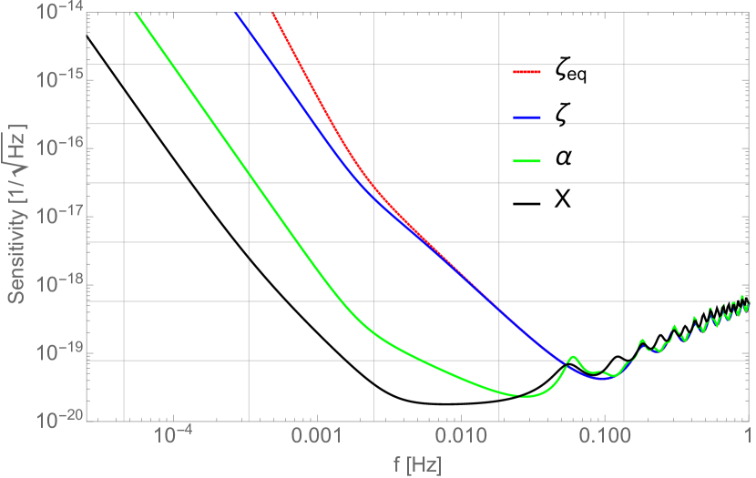
Figure 1: Gravitational wave strain noise spectral density calculation for TDI combinations X, $\alpha$, $\zeta$ averaged over sky position and polarization (see appendix D). The sensitivity are computed considering equal armlength for X and $\alpha$, while for $\zeta$ we also include the sensitivity for three unequal fixed armlength.

We can do a preliminary calculation by computing the total noise PSDs for TDI X and $\zeta$, which we denote as $S^{noise}_{X}$ and $S^{noise}_{\zeta}$. We compute them as the linear sum of the OMS and TM acceleration noises, respectively, using the low-frequency expansions given in eqs. 4 and 5. We get

$$S^{noise}_{X} \approx 64\tau^{4}\omega^{4}\bigg{(}4\sum_{ij\in\mathcal{I}_{X}}S_{g_{ij}}^{disp}+\sum_{ij\in\mathcal{I}_{X}}S_{oms_{ij}}\bigg{)},$$ (6)

$$S^{noise}_{\zeta} \approx\tau^{2}\omega^{2}\bigg{(}\tau^{2}\omega^{2}\sum_{ij\in\mathcal{I}_{\zeta}}S_{g_{ij}}^{disp}+\sum_{ij\in\mathcal{I}_{\zeta}}S_{oms_{ij}}\bigg{)},$$ (7)

as the overall noise entering in the two channels, valid for $\omega\tau\ll 1$. Here, we introduced the index sets $\mathcal{I}_{X}=\{12,21,13,31\}$ and $\mathcal{I}_{\zeta}=\{12,23,31,13,32,21\}$ for the four and six optical links (received at spacecraft i from spacecraft j) and TM acceleration noise terms ( TM in spacecraft i accelerated towards spacecraft j) appearing in X and $\zeta$, respectively.

We can observe that a TM displacement due to TM acceleration noise and the OMS noise enter with almost the same transfer function into the X channel, up to an additional factor 4 in the TM displacement. Conversely, in $\zeta$ the TM acceleration noise is suppressed towards low frequencies by a factor $\tau^{2}\omega^{2}$ relative to the OMS noise. This implies that while TM acceleration noise becomes dominant in X for frequencies in which (on average) $S_{oms}\ll 4S^{disp}_{g}$, for $\zeta$ the same holds only if $S_{oms}\ll\tau^{2}\omega^{2}S^{disp}_{g}$. Considering frequencies in the range ${10}^{-3}\text{\,}\mathrm{Hz}{10}^{-4}\text{\,}\mathrm{Hz}$, the TM acceleration noise pre-factor $\tau^{2}\omega^{2}$ (cf. eq. 7) is between $2.7\text{\times}{10}^{-5}2.7\text{\times}{10}^{-3}$. This means that the OMS noise would have to be from ten parts in a million to one part in a thousand smaller in power than the TM acceleration noise in order for the latter to have the same order of magnitude as the OMS noise in the $\zeta$ channel in the sub-$\mathrm{mHz}$ band.
As such, the null channels ability to monitor noise in the GW sensitive channels at low frequencies is limited. $\zeta$ could only be used to reliably detect the relevant sub-mHz noise in a worst case scenario where the TM acceleration noise is orders of magnitude larger than the OMS noise in these frequency ranges, such that it overcomes the scaling factor $\tau^{2}\omega^{2}$ and becomes dominant in both $\zeta$ and X.

As we will discuss in the next section, the currently assumed requirements for TM acceleration and OMS noises are very far away from these values. Nevertheless, we can still formulate upper and lower bounds on a SGWB signal based on X and $\zeta$ for the full LISA frequency band.

IV Upper limits, expected noise levels and simulations

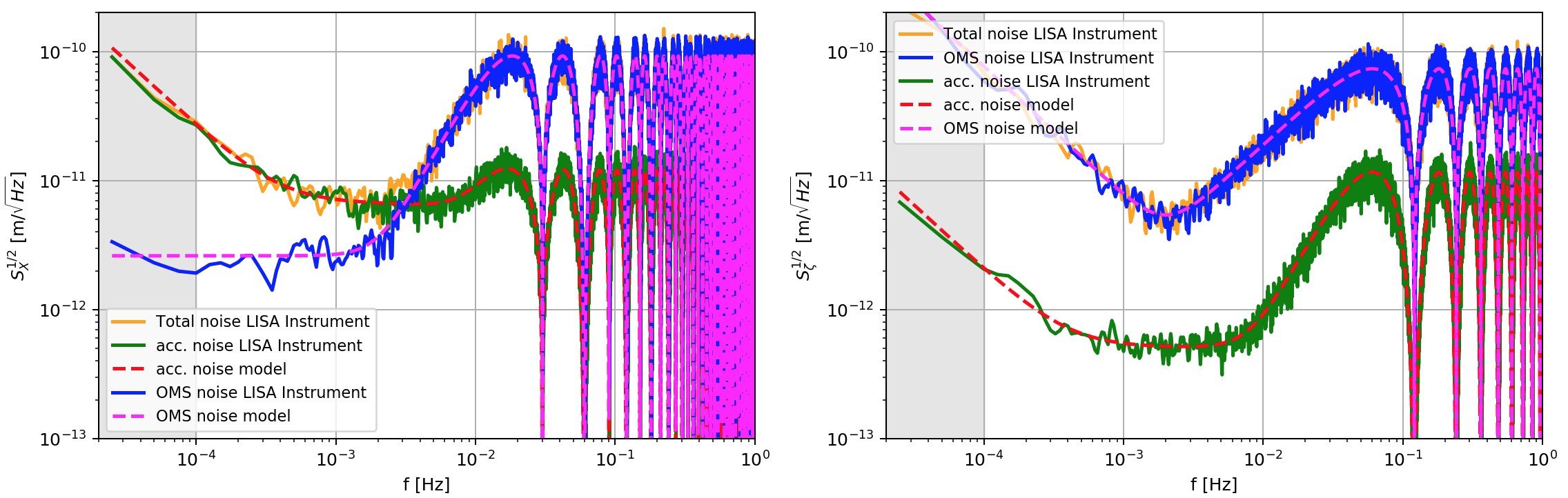
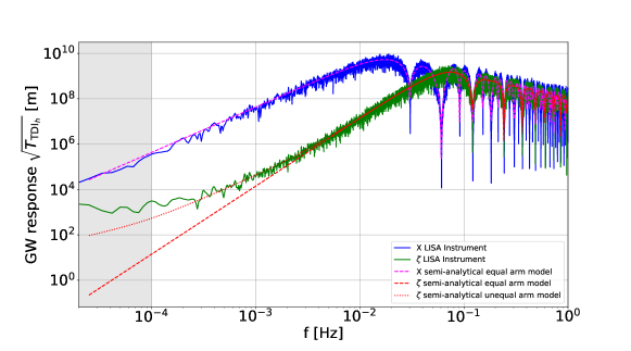
Figure 2: Upper plots: the left one shows the PSD of the TDI X and the right one the PSD of $\zeta$ for the TM acceleration noise, the optical metrology noise and the total noise as simulated with LISA Instrument compared with the respective analytical models. Lower plot: response to GW for TDI X and $\zeta$ as simulated with LISA Instrument and LISA GW-Response compared with the semi-analytical models computed considering equal armlength for X and both equal and three fixed unequal armlength for $\zeta$ as described in appendix D.

After the preliminary analysis in section III, let us now drop the low-frequency approximation and discuss the accuracy to which we can use X, $\alpha$ and $\zeta$ to identify a potential SGWB with LISA.

To this end, we briefly introduce the currently assumed noise levels given in the literature Babak et al. (2021). Note that these should be thought of as the performance requirements we aim to reach with as much margin as possible, not as accurate predictions of the actual in-flight performance.
We also perform time domains simulations using LISA Instrument Bayle (2022) and pyTDI Staab et al. (2022) to test our expressions for how these noises couple into the different TDI variables. Similarly, we also perform time domain simulations to test our semi-analytical computation of the GW response of different TDI variables presented in appendix D, using the tool GW-response Bayle et al. (2022a). Using simulations allows us to compare our (semi)-analytical expressions, computed assuming equal arm-lengths, with data generated using realistic LISA orbits provided by ESA.

IV.1 Analytical model and simulations

IV.1.1 Instrumental Noise

Considering the analytical computation in time domain of the TM acceleration and OMS noises for the TDI X, $\alpha$, $\zeta$ in appendix C, we can estimate the PSD of the aforementioned TDI combinations assuming all TM acceleration and OMS noises to be uncorrelated, which yields

$$S_{X_{g}}= \underbrace{256\sin^{4}(\tau\omega)\cos^{2}(\tau\omega)}_{T_{X_{g}}}\left(\left(S_{g_{12}}^{disp}+S_{g_{13}}^{disp}\right)\cos^{2}(\tau\omega)+S_{g_{21}}^{disp}+S_{g_{31}}^{disp}\right),$$ (8a)

$$S_{\alpha_{g}}= 16\sin^{2}\left(\frac{\tau\omega}{2}\right)\sin^{2}\left(\frac{3\tau\omega}{2}\right)\left((1+2\cos(\tau\omega))^{2}\left(S_{g_{12}}^{disp}+S_{g_{13}}^{disp}\right)+S_{g_{21}}^{disp}+S_{g_{23}}^{disp}+S_{g_{31}}^{disp}+S_{g_{32}}^{disp}\right),$$ (8b)

$$S_{\zeta_{g}}= \underbrace{16\sin^{4}\left(\frac{\tau\omega}{2}\right)}_{T_{\zeta_{g}}}\left(S_{g_{12}}^{disp}+S_{g_{13}}^{disp}+S_{g_{21}}^{disp}+S_{g_{23}}^{disp}+S_{g_{31}}^{disp}+S_{g_{32}}^{disp}\right),$$ (8c)

and

$$S_{X_{oms}}= \underbrace{64\sin^{4}(\tau\omega)\cos^{2}(\tau\omega)}_{T_{X_{oms}}}\left(S_{\text{oms}_{12}}+S_{\text{oms}_{13}}+S_{\text{oms}_{21}}+S_{\text{oms}_{31}}\right),$$ (9a)

$$S_{\alpha_{oms}}= 4\sin^{2}\left(\frac{3\tau\omega}{2}\right)\left(S_{\text{oms}_{12}}+S_{\text{oms}_{13}}+S_{\text{oms}_{21}}+S_{\text{oms}_{23}}+S_{\text{oms}_{31}}+S_{\text{oms}_{32}}\right),$$ (9b)

$$S_{\zeta_{oms}}= \underbrace{4\sin^{2}\left(\frac{\tau\omega}{2}\right)}_{T_{\zeta_{oms}}}\left(S_{\text{oms}_{12}}+S_{\text{oms}_{13}}+S_{\text{oms}_{21}}+S_{\text{oms}_{23}}+S_{\text{oms}_{31}}+S_{\text{oms}_{32}}\right).$$ (9c)

We verify the validity of these equations (derived in the equal-arm limit) using time domain simulations with realistic orbits. We disabled all noise sources available in LISA Instrument except TM acceleration noise and OMS noise in the inter-spacecraft interferometer, and set all noises of the same type to the same level, as given in Babak et al. (2021).

For the TM acceleration noises, this means a value of

$$S_{g_{ij}}(f)=\left(3\times 10^{-15}~{}\frac{\textrm{m}}{\textrm{s}^{2}~{}\sqrt{\textrm{Hz}}}\right)^{2}\times\left(1+\left(\frac{0.4~{}\textrm{mHz}}{f}\right)^{2}\right)\left(1+\left(\frac{f}{8~{}\textrm{mHz}}\right)^{4}\right),$$ (10)

which translates to

$$S_{g_{ij}}^{disp}(f)=S_{g_{ij}}(f)/(2\pi f)^{4}$$ (11)

in terms of displacement.

The noise level of the OMS is instead given as

$$S_{oms_{ij}}(f)=\left(15~{}\textrm{pm}/\sqrt{\textrm{Hz}}\right)^{2}\times\left(1+\left(\frac{2~{}\textrm{mHz}}{f}\right)^{4}\right),$$ (12)

where the factor $1+\left(\frac{2~{}\textrm{mHz}}{f}\right)^{4}$ is a low frequency relaxation term introduced to take into account our difficulties in measuring that noise below a few mHz from on-ground laboratory experiments. This relaxation is further justified by the fact that it has no impact on the low frequency GW sensitivity in X, as OMS noise remains very subdominant in X compared to TM acceleration noise even when including this factor, as visible in the left plot in fig. 2. Note that the estimated OMS noise model for LPF also includes a low-frequency relaxation to account for possible thermally driven effects Armano et al. (2021). However, these were likely buried in the LPF noise at lower frequencies where TM acceleration noise is believed to dominate. The upper part of fig. 2 shows the results of three simulation runs with LISA Instrument where we enable either one, the other or both of these noise sources. We use PyTDI to compute the Michelson X and $\zeta$ variables.

First, we note that in all cases, the simulated data, with realistic, unequal arm orbits, agrees well with the simplified equal-arm analytic expressions derived for the noise. We see that in the $\zeta$ channels the OMS noise is dominant over the TM acceleration noise at all frequency, while TM acceleration noise becomes the dominant noise source for X below a few $\mathrm{mHz}$.

Moreover, if we assume all noises of the same type to have the same noise level, we can use eqs. 9c and 8c to compute that for $\zeta$ we would need an OMS noise level of $S_{\zeta_{oms}}=24\sin^{2}(\frac{\tau\omega}{2})\times 4\sin^{2}(\frac{\tau\omega}{2})S_{g}^{disp}$ such that OMS and TM acceleration noises appear at the same magnitude. This can be translated in the single link OMS noise contribution with the value of $4\sin^{2}(\frac{\tau\omega}{2})S_{g}^{disp}$, which we compare in fig. 3 to the requirement for the OMS noise given in eq. 12.

We observe that this noise level is likely impossible to achieve as the new required level of OMS noise is $160\text{\,}\mathrm{p}\mathrm{m}\mathrm{/}\sqrt{\mathrm{Hz}}$ at $0.1\text{\,}\mathrm{mHz}$, orders of magnitude below the currently assumed value. It must be also kept in mind that this conclusion is true keeping fixed the TM acceleration noise level to the nominal value, while drastically lowering the OMS noise level. Any improvement of the TM acceleration noise in LISA would make the upper limit achieved by the null channel even less relevant.

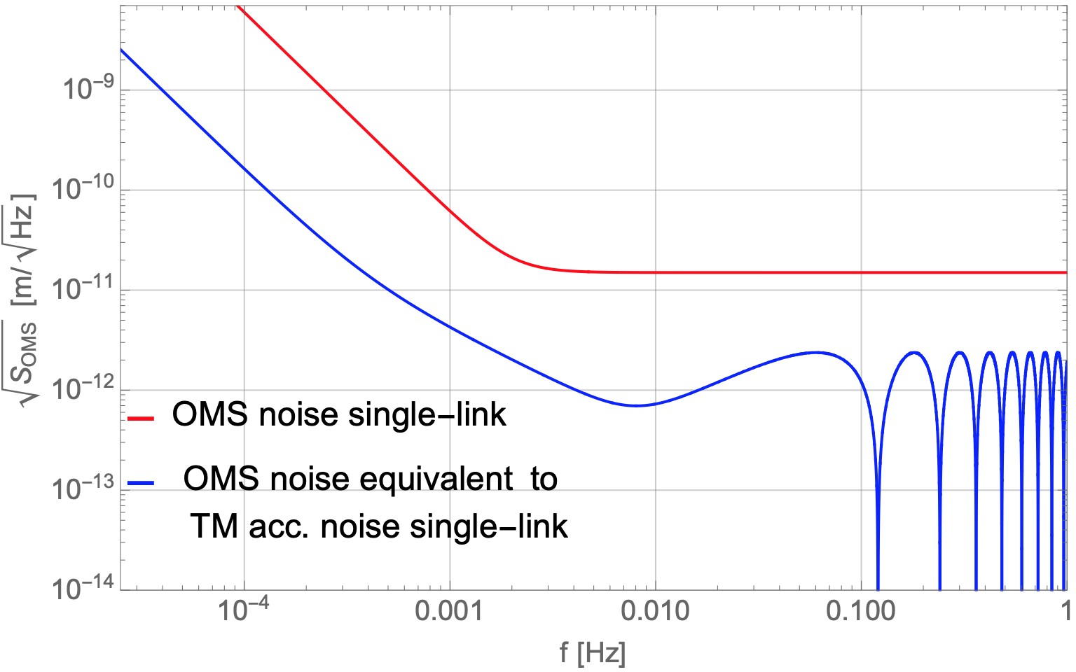
Figure 3: Comparison between the ASD of the optical metrology noise given in Babak et al. (2021) and the equivalent metrology noise in a single LISA link which would be required for the test mass acceleration noise to be dominant in the null channel $\zeta$.

However, fig. 2 shows that, at least assuming nominal noise levels, both X and $\zeta$ are dominated by OMS noise above 4 mHz, which might suggest that $\zeta$ can put a stronger constraint on the instrumental noise in this frequency range.

IV.1.2 Gravitational wave response

We denote the PSD of the X and $\zeta$ channels due to GWs as

$$S_{X_{h}}=T_{X_{h}}S_{h},\qquad S_{\zeta_{h}}=T_{\zeta_{h}}S_{h}.$$ (13)

$S_{h}$ is expressed as a dimensionless stochastic GW strain in ${\mathrm{Hz}}^{-1}$, while $S_{X_{h}}$ and $S_{\zeta_{h}}$ are expressed in $\mathrm{m}\mathrm{{}^{2}}\mathrm{/}\mathrm{Hz}$. Therefore, the response functions $T_{X_{h}}$ and $T_{\zeta_{h}}$ each include a conversion factor that has units ${\mathrm{m}}^{2}$.

The lower plot in fig. 2 shows the GW responses to a SGWB of TDI X and $\zeta$ for 51 stochastic GW sources isotropically distributed over the sky, computed in the frequency domain as described in appendix D. To verify the validity of these equal arm-length models, we compare them to time domain simulations using the tools LISA Instrument, GW-response and PyTDI which use realistic ESA orbits. We inject an isotropic SGWB computed from $N=48$ sources into the time-domain simulation and disable all instrumental noises. The two strain time series $h_{+}$, $h_{\times}$ for each source are computed as a white noise of amplitude $1/N$, where N is the number of GW sources, to overall simulate a sky-averaged response to a unit amplitude SGWB.

We see that for X our model for equal arms agrees with the simulations, while the equal arm-length model for $\zeta$ diverges from the simulations for frequencies smaller than 60 mHz. Considering three un-equal but constant arms for our semi-analytical response calculation for $\zeta$ extends the validity of the model to almost the entire LISA required frequency range, while we still see a divergence between simulations and the model at very low frequencies below $0.3\text{\,}\mathrm{mHz}$. A preliminary study indicates that the mismatch is probably linked to the fact that we neglect the Sagnac effect in our model, i.e., that we assume the delays accross the two directions of each arm to be equal.

However, as the mismatch mostly occurs outside the required LISA frequency band and the response of $\zeta$ remains sufficiently small compared to that of X inside the LISA band down to $0.1\text{\,}\mathrm{mHz}$ this does not significantly impact our conclusions.

IV.2 Combining Sagnac channels

First, let us consider the apparent possibility to use $\zeta$ to characterize and subtract the noise in $\alpha$. As discussed in section II.3.2, the OMS noise contributions in $\alpha$ and $\zeta$ fulfill $\alpha_{oms}(\tau)\approx 3\zeta_{oms}(\tau)$ at low frequencies. This implies that subtracting $3\zeta$ from $\alpha$ allows you to remove the common OMS noise. In fig. 4 we report the simulations of the TM acceleration noise plus OMS noise for $\alpha-3\zeta$ compared to the respective analytical models, which confirms what was predicted by the analytical calculation. What is then left as dominant noise source at low frequencies is a combinations of the following four TMs:

$$\begin{split}[\alpha_{oms,g}&-3\zeta_{oms,g}](t)\\ &\approx 6T^{2}\Big{(}{x^{g}_{12}}^{\prime\prime}(t)-{x^{g}_{13}}^{\prime\prime}(t)+{x^{g}_{21}}^{\prime\prime}(t)-{x^{g}_{31}}^{\prime\prime}(t)\Big{)}.\end{split}$$ (14)

We notice that eq. 14 is equal, up to a constant factor, to the low frequency TM acceleration noise of the TDI X channel (see eq. 4a). This means that using the null channel $\zeta$ to reduce the noise, with the purpose of retrieving the GW signal in $\alpha$, gives you back the channel X, which is sensitive to GWs as well as to the TM acceleration noise. We therefore focus on just the X and $\zeta$ channels in the following.

IV.3 Upper limit on instrumental noise in X

Let us now consider the expression for the OMS noise and TM acceleration noise for TDI $\zeta$ and X without considering the presence of GW signals in our data. To put an upper limit on the instrumental noise in X we are looking for a frequency dependent factor $F$ such that $FS_{\zeta}\geq S_{X}$, which implies

$$F(S_{\zeta_{oms}}+S_{\zeta_{g}})\geq S_{X_{oms}}+S_{X_{g}}.$$ (15)

Referring to eqs. 9a, 9c, 8a and 8c, this means

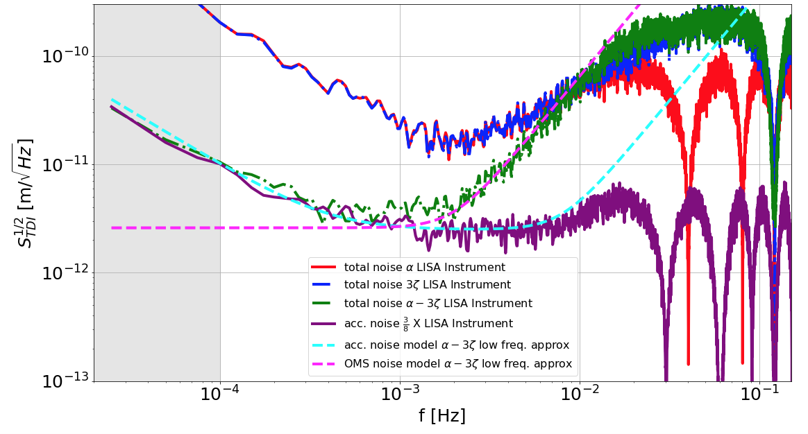
Figure 4: Amplitude spectral density of the TDI $\alpha$, 3$\zeta$ and $\alpha-3\zeta$ for the acceleration noise and metrology noise. For TDI X only the amplitude spectral density of the acceleration noise is shown. The simulations use realistic ESA orbits included with Bayle et al. (2022b) while the models are derived assuming equal arms and considering only the low frequency component of the acceleration and metrology noise for the TDI combination $\alpha-3\zeta$.

$$FT_{\zeta_{oms}}\sum_{ij\in\mathcal{I}_{\zeta}}S_{\text{oms}_{ij}}+FT_{\zeta_{g}}\sum_{ij\in\mathcal{I}_{\zeta}}S_{g_{ij}}^{disp}\geq T_{X_{oms}}\sum_{ij\in\mathcal{I}_{X}}S_{\text{oms}_{ij}}+T_{X_{g}}\left(\left(S_{g_{12}}^{disp}+S_{g_{13}}^{disp}\right)\cos^{2}(\tau\omega)+S_{g_{21}}^{disp}+S_{g_{31}}^{disp}\right).$$ (16)

Since $\mathcal{I}_{X}\subset\mathcal{I}_{\zeta}$ and $S_{\text{oms}_{ij}}$ and $S_{\text{g}_{ij}}$ are strictly positive, we have

$$\sum_{ij\in\mathcal{I}_{\zeta}}S_{\text{oms}_{ij}}\geq\sum_{ij\in\mathcal{I}_{X}}S_{\text{oms}_{ij}}$$ (17)

and further considering that $\cos^{2}(\tau\omega)\leq 1$ we get

$$\sum_{ij\in\mathcal{I}_{\zeta}}S_{g_{ij}}^{disp}\geq\left(\left(S_{g_{12}}^{disp}+S_{g_{13}}^{disp}\right)\cos^{2}(\tau\omega)+S_{g_{21}}^{disp}+S_{g_{31}}^{disp}\right).$$ (18)

We see that $F(S_{\zeta_{oms}}+S_{\zeta_{g}})\geq S_{X_{oms}}+S_{X_{g}}$ is valid as long as

$$F\geq T_{X_{oms}}/T_{\zeta_{oms}}\qquad\mathrm{and}\qquad F\geq T_{X_{g}}/T_{\zeta_{g}}.$$ (19)

We can therefore define our noise estimate factor as

$$F=\mathrm{Max}(T_{X_{oms}}/T_{\zeta_{oms}},T_{X_{g}}/T_{\zeta_{g}})=256\cos^{4}\left(\frac{\omega\tau}{2}\right)\cos^{2}(\omega\tau).$$ (20)

Note that by inspection of eqs. 8a, 8c, 9a and 9c), we find the ratio $T_{X_{g}}/T_{\zeta_{g}}$ to be dominant at all frequencies, which allows us evaluate the maximum in the previous equation.

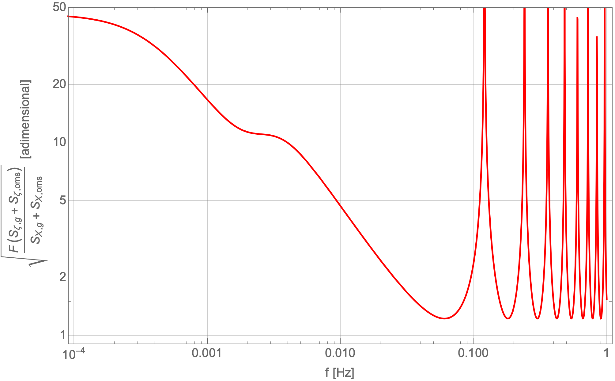
Figure 5: Left: Upper limit on the instrumental noise in X derived from the noise observed in $\zeta$, for the case where all TM acceleration and optical metrology noises are at the levels specified by eqs. 11 and 12, respectively. Moreover, the dotted yellow and blue curves show the estimate one could put on just the OMS or TM noise, respectively. Right: Ratio between actual noise in X and the overall upper limit, in amplitude assuming required levels of TM acceleration and OMS noise.

We show in fig. 5, in the left plot, the overall noise upper limit $FS^{noise}_{\zeta}$ obtained in this way next to the actual noise $S^{noise}_{X}$ in X. In addition, we show the two individual upper limits we would obtain for just the OMS noise and just the TM acceleration noise by considering only the contribution of $\frac{T_{X_{oms}}}{T_{\zeta_{oms}}}S^{noise}_{\zeta}$ and $\frac{T_{X_{g}}}{T_{\zeta_{g}}}S^{noise}_{\zeta}$, respectively.

Inspecting the right plot of fig. 5, we observe that (assuming noise at the required levels) the upper limit on the instrumental noise in X posed by $\zeta$ is up to a factor 50 in amplitude above the actual noise level, in particular at low frequencies. This results in a rather weak upper limit, reflecting OMS noise in a frequency band where only TM acceleration noise is relevant. At high frequencies, on the other hand, where both X and $\zeta$ are dominated by OMS noise, the estimate is significantly more stringent, and stays below a factor 2 in amplitude from 25 to $100\text{\,}\mathrm{mHz}$.

We want to underline that the derivation of the expression $FS^{noise}_{\zeta}$ for the noise upper limit does not rely on any assumptions on the actual noise levels of the individual TM and OMS noise terms, as only sums over all TM and OMS channels affects eq. 16. Additionally, it could be evaluated at any time, and is therefore robust against non-stationarity of the noise. However, this upper limit does rely on our assumptions on noise correlations made in section II, and the particular outcome we show in fig. 5 reflects the nominal values assumed for the level of TM acceleration and OMS noise.

IV.4 Upper and lower limits on a SGWB

We now additionally consider the presence of possible SGWBs in our data, on which we can put lower and upper bounds as follows. As before for the instrumental noise, we will remain agnostic to the spectral shape and amplitude of the SGWB. We do however assume to know the response function of the different TDI channels, which we compute as described in appendix D for the case of an isotropic SGWB.

In the presence of such a SGWB we can introduce

$$S^{meas}_{X}=S^{noise}_{X}+S_{X_{h}},$$ (21)

as the combination of instrumental noise and GW signal that we can actually measure in the TDI X channel.

We remind that eq. 13 together with eq. 21 immediately allows us to put an upper bound on a possible SGWBs,

$$S_{h}\leq S^{meas}_{X}/T_{X_{h}},$$ (22)

as any model predicting a higher value of $S_{h}$ would be incompatible with our measurements $S^{meas}_{X}$.

To put a lower bound on $S_{h}$ based on our data (i.e., claim a detection), we can make use of our previously derived upper bound $FS^{noise}_{\zeta}$ on the instrumental noise in X.

To this end, as $\zeta$ is not perfectly insensitive to GWs (cf. fig. 1), we need to define

$$S^{meas}_{\zeta}=S^{noise}_{\zeta}+S_{\zeta_{h}}.$$ (23)

The upper bound (cf. eq. 15) on the instrumental noise now becomes $F(S^{meas}_{\zeta}-S_{\zeta_{h}})\geq S^{noise}_{X}$, which allows us to write

$$S^{meas}_{X}\leq F(S_{\zeta}^{meas}-S_{\zeta_{h}})+S_{X_{h}},$$ (24)

where we simply add $S_{X_{h}}$ on both sides of the previous inequality and consider the definition of $S^{meas}_{X}$. Then, considering eq. 13 this implies the lower bound

$$S_{h}\geq\frac{S^{meas}_{X}-FS^{meas}_{\zeta}}{T_{X_{h}}-FT_{\zeta_{h}}},\quad\text{valid if $T_{X_{h}}>FT_{\zeta_{h}}$}.$$ (25)

Note that the right-hand side of this equation can be negative even if there is a SGWB, in which case it is compatible with $S_{h}=0$ and we cannot claim a detection of a SGWB. On the other hand, if it is positive, this would indicate presence of a GW background, at least in the assumptions used here.

Assuming that we only consider the frequency range in which eq. 25 is valid, i.e., if $T_{X_{h}}>FT_{\zeta_{h}}$, the right-hand side of eq. 25 will be positive if $S^{meas}_{X}>FS^{meas}_{\zeta}$, which means we are able to identify a SGWB if

$$S^{noise}_{X}+T_{X_{h}}S_{h} >F(S^{noise}_{\zeta}+T_{\zeta_{h}}S_{h})$$ (26a)

$$\iff S_{h} >\frac{FS^{noise}_{\zeta}-S^{noise}_{X}}{T_{X_{h}}-FT_{\zeta_{h}}}.$$ (26b)

Equation 26b allows us to define a detection threshold assuming known noise levels, as depicted in the left plot of fig. 6, where it is shown alongside the upper limit defined in eq. 22 in case we don’t have a GW background. Note that both these quantities now apply to the fundamentally unknowable instrumental noise levels, and cannot be evaluated from the raw data.

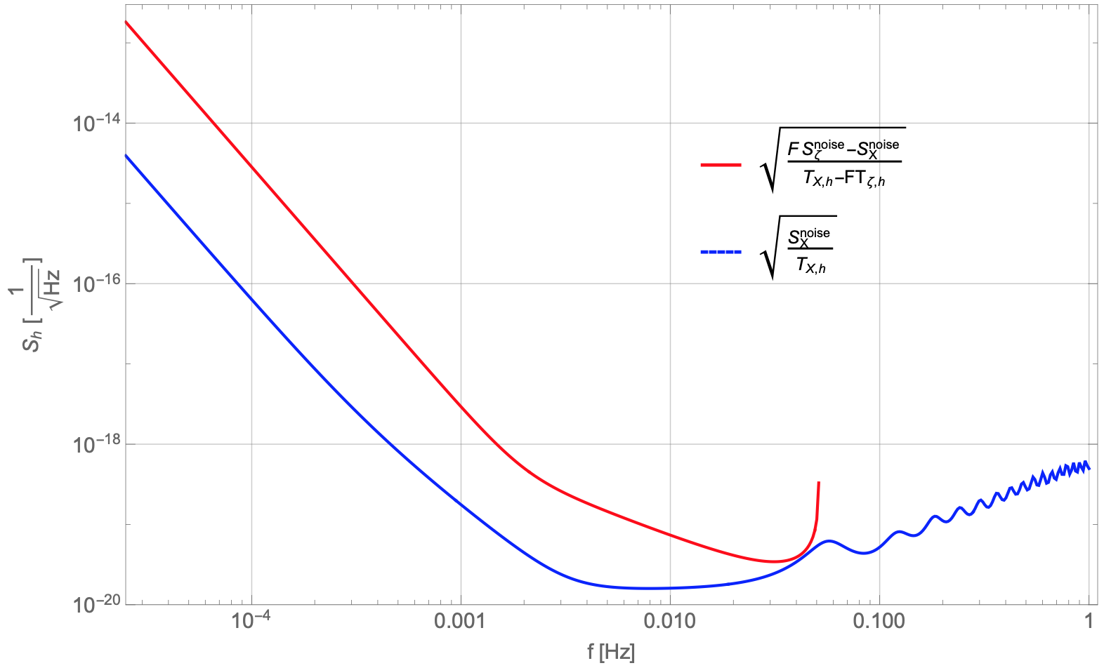
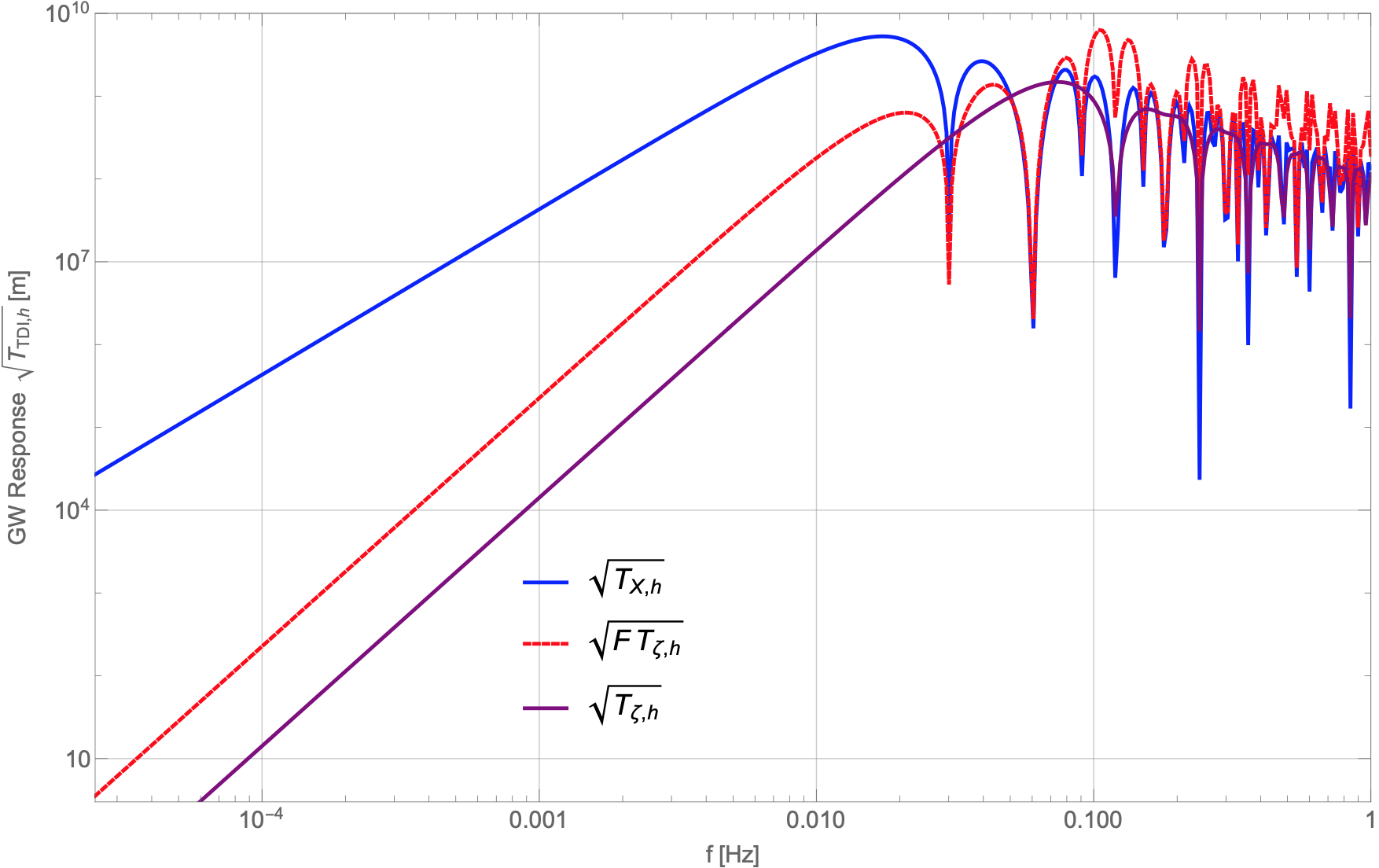
Figure 6: Left: Comparison of the detection threshold derived from $\zeta$ (red curve) and the upper limit given by X (blue curve), both expressed as relative armlength change (strain) assuming OMS and TM acceleration noise at the requirements level. Right: GW response functions of TDI X, $FS_{\zeta}$ and $S_{\zeta}$, computed assuming 51 stochastic GW sources isotropicaly distributed over the sky.

We remind that the scaling factor $F$ used in this derivation was computed in the equal-arm assumption. While we showed in section IV.1 that the equal-arm noise models are generally valid across most of the LISA frequency band, we expect them to diverge in small frequency bands around the zeros of the TDI transfer function.

This issue might be circumvented by using a different set of second generation TDI variables which lack zeros at such low frequencies, as for example described in Hartwig and Muratore (2022).

V Conclusion

The LISA data analysis, particularly in the search for a SGWB, should be as robust as possible to ignorance of the noise model and to variations of the noise from the different components of the instrumental setup.

It will likely be impossible to accurately predict and faithfully model the instrumental noise performance pre-flight, such that efforts to characterize the noise based on in-flight observables should be exploited as much as possible. We present here how one can use the $\zeta$ channel to estimate the level at which two of the main noise sources, the uncorrelated TM acceleration and OMS noise, will affect the GW sensitive X channel. This is a rather conservative estimate, in the sense that it assumes nothing about actual instrumental noise levels, homogeneity between different TM acceleration or OMS noise terms and noise stationarity. However, there are potential limits due to our assumptions on noise correlations, as $\zeta$ is highly insensitive to correlated noise entering both single-link measurements on-board a single spacecraft, while X is not.

We show that using $\zeta$ we estimate the noises under consideration in X within a factor 2 in amplitude in the band from $25\text{\,}\mathrm{mHz}$ to $100\text{\,}\mathrm{mHz}$, while this estimate worsens to within a factor $50$ in amplitude at the lowest frequencies (assuming the instrumental noise levels from the requirement). We can use this upper bound on the instrumental noise to compute a lower bound on the GW background needed to explain the overall observed PSDs of both $\zeta$ and X. To this end, both the response of X to gravitational waves, $T_{X,h}$, and that of our instrumental noise estimate to gravitational waves, $FT_{\zeta,h}$, have to be considered. While $FT_{\zeta,h}$ is strongly subdominant to $T_{X,h}$ at low frequencies, this relationship is inverted at high frequencies, such that the lower bound becomes less stringent than one would expect from the performance of the noise estimate alone, and eventually becomes invalid. As visible in the right plot of fig. 6, we have $T_{X_{h}}>FT_{\zeta_{h}}$ only up to around $50\text{\,}\mathrm{mHz}$.

Note that the fact that the noise estimate $\zeta$ provides at low frequencies is a factor 50 above the actual instrumental noise in X implies that, within the assumption of this study, we could identify a SGWB only if it were significantly larger than the TM acceleration noise expected to dominate X at these frequencies.

Still, even assuming the nominal instrumental noise levels, this lower bound would allow to detect big stochastic backgrounds in a large part of the frequency band. Given the large uncertainties in the range of possible stochastic background levels Caprini and Figueroa (2018), including spectral shape and amplitude, as well as the demonstrated difficulty in predicting instrument noise, the results shown here might proof useful. As such, our paper addresses the idea of simultaneous signal plus noise measurement, and shows the limit of achieving this with the TDI null channel.

Note that while our approach is agnostic to the noise levels, the predicted performance is computed assuming OMS noise to be exactly at the required noise levels (which includes a strong low-frequency relaxation), but, especially at low frequency, this noise has high uncertainty. If the actual hardware turns out to perform better in-flight than what can be demonstrated on-ground, the estimate would consequently improve. For example, earlier studies which performed similar estimates (e.g., Tinto et al. (2001), Hogan and Bender (2001b)) assumed the OMS noise to be white across the whole frequency band, and came to the conclusion that we can make a better use of the null channels at low frequencies to estimate the SGWB. We remark that for the OMS noise in $\zeta$ to reach the same level as the TM acceleration noise (limiting the X channels at low frequencies) would require order of magnitude improvements in the performance of the OMS.

We want to reinforce that the upper and lower bounds we compute here are agnostic to the actual instrument performance and don’t rely on any model of the individual noise spectral shapes or stationarities. This is in contrast to some other results in the literature (see for instance Adams and Cornish (2010, 2014); Caprini et al. (2019); Flauger et al. (2021); Wang et al. (2022)), which showed it is possible to put significantly more stringent bounds on the noise assuming stationarity over the whole mission duration and a fixed (and known) noise shape which only depends on a single amplitude parameter. If indeed such a priori knowledge of the noise level and shape were possible, it would be possible to resolve SGWB even below the threshold of the instrument noise.

The results presented here demonstrate the necessity of using realistic assumptions on the prior knowledge of the instrumental noise, noise correlations and stationarity. It is important to consider that the data analysis pipelines in LISA operations will likely rely on some model for the noise (even if Bayesian techniques for parameter’s estimation with unknown noise has been introduced in literature, see for instance Vitale et al. (2014) ). Although procedures like those described in this manuscript do not translate naturally into a Bayesian data analysis framework we believe they might still proof useful to cross-check and interpret the results from a full Bayesian analysis, given the large number of parameters such a procedure has to determine. Additionally, the lower and upper bounds provided from our method could be used as priors in a Bayesian framework.

Further studies should be performed to quantify the real impact this has on achieving the LISA science objectives to detect SGWBs.

To conclude, we reiterate that this study is limited in that we only considered the two main classes of noise, TM acceleration and OMS noise, and that we further assume that these are fully uncorrelated for the six TMs and six one-way optical metrology links. Follow-up studies could investigate other known noise sources with different correlation properties, such as sideband modulation noise Hartwig and Bayle (2021) or TTL couplings Paczkowski et al. (2022), to verify to which extend the results presented here hold for such noises. Furthermore, we only considered here the case of an isotropic SGWB for simplicity. Any anisotropic SGWB, such as the expected foreground from galactic binaries, will have an annual modulation in the response function, which might help to distinguish it better from the instrumental noise. We want to remark that some instrumental noises might also show annual modulations due to the position of the LISA satellites along the orbit, which one should account for when studying this scenario.

VI Acknowlegement

We thank the LISA simulation working group, in particular Jean-Baptiste Bayle, Quentin Baghi, Maude Le Jeune, Arianna Renzini and Martin Staab for developing the tools used for the simulations. We also thank the anonymous referee for the useful comments on improving the manuscript. M.M and O.H. want to thank Antoine Petiteau, Mauro Pieroni, Marc Lilley and Jonathan Gair for interesting discussions regarding this topic. M.M, S.V, D.V. and W.J.W. thank the LISA Trento group for the fruitful discussion and the Istituto Nazionale di Fisica Nucleare (INFN) for supporting this work. This work was funded by the Agenzia Spaziale Italiana (ASI), Project No. 2017-29-H.1-2020 ”Attività per la fase A della missione LISA”. O.H. gratefully acknowledges support by the Centre national d’études spatiales. This work was supported by the Programme National GRAM of CNRS/INSU with INP and IN2P3 co-funded by CNES. M.M. gratefully acknowledge support by the Deutsches Zentrum fur Luft- und Raumfahrt (DLR) with funding from the Bundesministerium fur Wirtschaft und Technologie (Project Ref. Number 50 OQ 1801)

Appendix A Time shift operators

We define the following notations related to time-shift operators and TDI combinations Hartwig and Muratore (2022):

Delay operator:

$$D_{ij}\eta(\tau)=\eta(\tau-d_{ij}(\tau)).$$ (27)

Given a time of reception $\tau$ of a beam on spacecraft $i$, evaluates the measurements $\eta$ (we dropped the double index for simplicity) of that beam at the time of emission at spacecraft $j$, which we write as $\tau-d_{ij}(\tau)$. Note that depending on what frame $\eta(\tau)$ is defined in, the computation of $d_{ij}$ can include a change in reference frames and clock offsets, as discussed in Hartwig et al. (2022).

Advancement operator:

$$A_{ij}\eta(\tau)=\eta(\tau+a_{ij}(\tau)).$$ (28)

Given a time of emission $\tau$ of a beam from spacecraft $j$, evaluates the phase $\eta$ of that beam at the time of reception on spacecraft $i$, which we write as $\tau+a_{ij}(\tau)$. This is the inverse operation to that of the delay operator, such that we have the identity $A_{ij}D_{ji}\eta(t)=D_{ij}A_{ji}\eta(t)=\eta(t)$.

Multiple Delay operators:

$$D_{ij}D_{jk}\eta(\tau)=\eta(\tau-d_{ij}(\tau)-d_{jk}(\tau-d_{ij}(\tau)).$$ (29)

Multiple Delay and Advancement operators:

$$\begin{split}A_{ni}D_{ij}&D_{jk}\eta(\tau)=\eta\Big{(}\tau+a_{ni}(\tau)-d_{ij}(\tau+a_{ni}(\tau))\\ &\quad-d_{jk}(\tau+a_{ni}(\tau)-d_{ij}(\tau+a_{ni}(\tau)))\Big{)}.\end{split}$$ (30)

Only the delays $d_{ij}(\tau)$ are directly accessible from the LISA measurements. The advancements $a_{ij}(\tau)$ can be computed from them by iteratively solving

$$a_{ij}(\tau)=d_{ji}(\tau+a_{ij}(\tau)),$$ (31)

which directly follows from $A_{ij}D_{ji}\eta(t)=\eta(t)$.

Appendix B TM acceleration and displacement noise models

Following the convention that $\vec{L}_{ji}$ is the link vector from the emitting satellite OBj to the receiving one OBi, and $\vec{g}_{i}$ the OBi acceleration relative to its inertial reference frame, we can define the acceleration of OBi that points towards OBj, at time t, as:

$$g_{ij}(t)\equiv\vec{g}_{i}(t)\cdot\hat{L}_{ji}.$$ (32)

Then, the relative acceleration $\Delta g_{\textrm{single-link}}(t)$, between the two free-falling TMs along the line of sight of the unit vector $\hat{L}_{ji}$, at time $t$ on $OB_{i}$, can be computed as:

$$\Delta{g_{\textrm{single-link}}}(t) =(\vec{g}_{i}(t)-\vec{g}_{j}(t-\tau))\cdot\hat{L}_{ji}$$ (33)

$$\equiv(g_{ij}(t)+g_{ji}(t-\tau)),$$ (34)

where we have use the approximation that:

$$\vec{g}_{i}(t)\cdot\hat{L}_{ji}\approx-\vec{g}_{i}(t)\cdot\hat{L}_{ij}.$$ (35)

We can estimate the PSD of $\Delta{g_{\textrm{single-link}}}$ under the assumption of uncorrelated but statistically equivalent acceleration noises for the two TMs as:

$$S_{\Delta{g_{\textrm{single-link}}}}(\omega)=2S_{g_{ij}},$$ (36)

where $S_{g_{ij}}$ is the PSD of the single TM acceleration noise. To give an estimate of the OMS noise for the inter-spacecraft interferometer in a LISA link, we should consider that it enters just at the time $t$ when we perform the measurement, as:

$$\Delta x_{\textrm{single-link}}(t)=x_{ij}(t).$$ (37)

Here $x_{ij}$ is the readout noise expressed in term of displacement at OBj that faces the far OBi.

Appendix C Analytical computation in time domain of the acceleration noise and displacement noise for the TDI X, $\alpha$, $\zeta$

We can compute how the TM acceleration noise propagates through the TDI X, $\alpha$ and $\zeta$, assuming equal and constant arm lengths as follows:

$$\begin{split}X_{g}(t)=&g_{12}(t-8\tau)-2g_{12}(t-4\tau)-g_{13}(t-8\tau)+2g_{13}(t-4\tau)+2g_{21}(t-7\tau)\\ &-2g_{21}(t-5\tau)-2g_{21}(t-3\tau)+2g_{21}(t-\tau)-2g_{31}(t-7\tau)+2g_{31}(t-5\tau)\\ &+2g_{31}(t-3\tau)-2g_{31}(t-\tau)+g_{12}(t)-g_{13}(t),\end{split}$$ (38a)

$$\begin{split}\alpha_{g}(\tau)=&g_{12}(t-6\tau)-2g_{12}(t-3\tau)-g_{13}(t-6\tau)+2g_{13}(t-3\tau)+g_{21}(t-5\tau)-g_{21}(t-4\tau)\\ &-g_{21}(t-2\tau)+g_{21}(t-\tau)+g_{23}(t-5\tau)-g_{23}(t-4\tau)\\ &-g_{23}(t-2\tau)+g_{23}(t-\tau)-g_{31}(t-5\tau)+g_{31}(t-4\tau)+g_{31}(t-2\tau)-g_{31}(t-\tau)\\ &-g_{32}(t-5\tau)+g_{32}(t-4\tau)+g_{32}(-2\tau)-g_{32}(t-\tau)+g_{12}(0)-g_{13}(0),\end{split}$$ (38b)

$$\begin{split}\zeta_{g}(t)=&g_{12}(t-2\tau)-2g_{12}(t-\tau)-g_{1,3}(t-2\tau)+2g_{13}(t-\tau)-g_{21}(t-2\tau)+2g_{21}(t-\tau)\\ &+g_{23}(t-2\tau)-2g_{2,3}(t-\tau)+g_{3,1}(t-2\tau)-2g_{31}(t-\tau)\\ &-g_{32}(t-2\tau)+2g_{32}(t-\tau)+g_{12}(t)-g_{13}(t)-g_{21}(t)+g_{23}(t)+g_{31}(t)-g_{32}(t).\end{split}$$ (38c)

Following the same assumption we used for computing the TM acceleration noise, we can also compute how the OMS noise enters in the above mentioned TDI channels:

$$\begin{split}X_{oms}(t)=&x_{12}(t-6\tau)-x_{12}(t-4\tau)-x_{12}(t-2\tau)-x_{13}(t-6\tau)+x_{13}(-4\tau)\\ &+x_{13}(t-2\tau)+x_{21}(t-7\tau)-x_{21}(t-5\tau)-x_{21}(t-3\tau)+x_{21}(t-\tau)\\ &-x_{31}(t-7\tau)+x_{31}(t-5\tau)+x_{31}(t-3\tau)-x_{31}(t-\tau)+x_{12}(t)-x_{13}(t),\end{split}$$ (39a)

$$\begin{split}\alpha_{oms}(t)=&-x_{12}(t-3\tau)+x_{13}(t-3\tau)+x_{21}(t-5\tau)-x_{21}(t-2\tau)\\ &-x_{23}(t-4\tau)+x_{23}(t-\tau)-x_{31}(t-5\tau)+x_{31}(t-2\tau)+x_{32}(t-4\tau)\\ &-x_{32}(t-\tau)+x_{12}(t)-x_{13}(t),\end{split}$$ (39b)

$$\begin{split}\zeta_{oms}(t)=&-x_{12}(t-\tau)+x_{13}(t-\tau)+x_{21}(t-\tau)-x_{23}(t-\tau)-x_{31}(t-\tau)\\ &+x_{32}(t-\tau)+x_{12}(t)-x_{13}(t)-x_{21}(t)+x_{23}(t)+x_{31}(t)-x_{32}(t).\end{split}$$ (39c)

Appendix D Computation of the Sensitivity

Following Muratore (2021) and Muratore et al. (2022), We consider stochastic sources with both plus and cross polarizations in their source frame. In the Solar System Barycenter (SSB), these will appear with $h_{+}(t,\textbf{r})$ and $h_{\times}(t,\textbf{r})$ given by $h^{SSB}_{+}(t,\textbf{r})=h_{+}(t,\textbf{r})\cos(2\psi)-h_{\times}(t,\textbf{r})\sin(2\psi)$ and $h^{SSB}_{\times}(t,\textbf{r})=h_{+}(t,\textbf{r})\sin(2\psi)+h_{\times}(t,\textbf{r})\cos(2\psi)$, where $\psi$ is the polarization angle. The sensitivity to GW sources coming from different directions is computed for each source considering the relative frequency shift that an incoming GW causes on a LISA link as for example given in Babak et al. (2021). We then convert this frequency shift to an equivalent displacement. We computed both the case of three equal armlength and three unequal constant armlength. Assuming that our signal is made of superposition of many GW sources coming from different directions and with different polarizations, we can consider that the output of a TDI_j, given superpositions of $n$ plane waves is:

$$S_{{j}_{h}}=\sum_{i}^{n}T_{j_{h}}^{i}(\omega)S_{h_{i}}(\omega),$$ (40)

where $S_{h_{i}}(\omega)$ is the PSD of the $i$’th GW source expressed as dimensionless strain, and $T_{j_{h}}^{i}(\omega)$ is the absolute squared value transfer function for the $j$’th TDI, including the conversion factor such that $S_{{j}_{h}}$ is in units of ${\mathrm{m}}^{2}\text{\,}{\mathrm{Hz}}^{-1}$. Labelling the PSD of the TM acceleration noise and OMS noise for each TDI $j$ as $S_{{j}_{g}}$ and $S_{{j}_{oms}}$, respectively, the sensitivity of each TDI combination is computed by renormalising the total instrument noise Amplitude Spectral Density (ASD) by the GW transfer function as:

$$S_{{j}_{n/h}}=\frac{S^{disp}_{{j}_{g}}+S_{{j}_{oms}}}{RMS\{T_{j_{h}}^{i}(\omega)\}},$$ (41)

where the $RMS\{\}$ denotes the root mean square over all sources $i$ and as before $S^{disp}_{{j}_{g}}$ is the TM acceleration noise expressed as an equivalent displacement.
The response to a SGWB can also be written using a continous integral over the whole sky as for example shown in Smith and Caldwell (2019) and Flauger et al. (2021). The angular integral reported there is then evaluated numerically to get a result which is valid for the whole LISA frequency range. The computation reported in this paper is one possible method for numerically approximating the result of the continous integral by replacing it with a sum over discrete stochastic sources from different directions. Indeed, in the limit of an infinite number of sources, this converges to the same integral.

References

- Amaro-Seoane et al. (2017) P. Amaro-Seoane, H. Audley, S. Babak, J. Baker, E. Barausse, P. Bender, E. Berti, P. Binetruy, M. Born, D. Bortoluzzi, J. Camp, C. Caprini, V. Cardoso, M. Colpi, J. Conklin, N. Cornish, C. Cutler, K. Danzmann, R. Dolesi, L. Ferraioli, V. Ferroni, E. Fitzsimons, J. Gair, L. G. Bote, D. Giardini, F. Gibert, C. Grimani, H. Halloin, G. Heinzel, T. Hertog, M. Hewitson, K. Holley-Bockelmann, D. Hollington, M. Hueller, H. Inchauspe, P. Jetzer, N. Karnesis, C. Killow, A. Klein, B. Klipstein, N. Korsakova, S. L. Larson, J. Livas, I. Lloro, N. Man, D. Mance, J. Martino, I. Mateos, K. McKenzie, S. T. McWilliams, C. Miller, G. Mueller, G. Nardini, G. Nelemans, M. Nofrarias, A. Petiteau, P. Pivato, E. Plagnol, E. Porter, J. Reiche, D. Robertson, N. Robertson, E. Rossi, G. Russano, B. Schutz, A. Sesana, D. Shoemaker, J. Slutsky, C. F. Sopuerta, T. Sumner, N. Tamanini, I. Thorpe, M. Troebs, M. Vallisneri, A. Vecchio, D. Vetrugno, S. Vitale, M. Volonteri, G. Wanner, H. Ward, P. Wass, W. Weber, J. Ziemer, and P. Zweifel, “Laser interferometer space antenna,” (2017).
- Armstrong et al. (1999) J. W. Armstrong, F. B. Estabrook, and M. Tinto, The Astrophysical Journal 527, 814 (1999).
- Hogan and Bender (2001a) C. J. Hogan and P. L. Bender, Phys. Rev. D 64, 062002 (2001a).
- Muratore et al. (2022) M. Muratore, D. Vetrugno, S. Vitale, and O. Hartwig, Phys. Rev. D 105, 023009 (2022).
- Muratore et al. (2020) M. Muratore, D. Vetrugno, and S. Vitale, Classical and Quantum Gravity 37, 185019 (2020).
- Hu and Wu (2017) W.-R. Hu and Y.-L. Wu, Natl. Sci. Rev. 4, 685 (2017).
- Littenberg and Cornish (2023) T. B. Littenberg and N. J. Cornish, “Prototype global analysis of lisa data with multiple source types,” (2023).
- Armano et al. (2018) M. Armano, H. Audley, J. Baird, P. Binetruy, M. Born, D. Bortoluzzi, E. Castelli, A. Cavalleri, A. Cesarini, A. M. Cruise, K. Danzmann, M. de Deus Silva, I. Diepholz, G. Dixon, R. Dolesi, L. Ferraioli, V. Ferroni, E. D. Fitzsimons, M. Freschi, L. Gesa, F. Gibert, D. Giardini, R. Giusteri, C. Grimani, J. Grzymisch, I. Harrison, G. Heinzel, M. Hewitson, D. Hollington, D. Hoyland, M. Hueller, H. Inchauspé, O. Jennrich, P. Jetzer, N. Karnesis, B. Kaune, N. Korsakova, C. J. Killow, J. A. Lobo, I. Lloro, L. Liu, J. P. López-Zaragoza, R. Maarschalkerweerd, D. Mance, N. Meshksar, V. Martín, L. Martin-Polo, J. Martino, F. Martin-Porqueras, I. Mateos, P. W. McNamara, J. Mendes, L. Mendes, M. Nofrarias, S. Paczkowski, M. Perreur-Lloyd, A. Petiteau, P. Pivato, E. Plagnol, J. Ramos-Castro, J. Reiche, D. I. Robertson, F. Rivas, G. Russano, J. Slutsky, C. F. Sopuerta, T. Sumner, D. Texier, J. I. Thorpe, D. Vetrugno, S. Vitale, G. Wanner, H. Ward, P. J. Wass, W. J. Weber, L. Wissel, A. Wittchen, and P. Zweifel, Phys. Rev. Lett. 120, 061101 (2018).
- Armano et al. (2016) M. Armano, H. Audley, G. Auger, J. Baird, P. Binetruy, M. Born, D. Bortoluzzi, N. Brandt, A. Bursi, M. Caleno, A. Cavalleri, A. Cesarini, M. Cruise, K. Danzmann, M. de Deus Silva, D. Desiderio, E. Piersanti, I. Diepholz, R. Dolesi, N. Dunbar, L. Ferraioli, V. Ferroni, E. Fitzsimons, R. Flatscher, M. Freschi, J. Gallegos, C. G. Marirrodriga, R. Gerndt, L. Gesa, F. Gibert, D. Giardini, R. Giusteri, C. Grimani, J. Grzymisch, I. Harrison, G. Heinzel, M. Hewitson, D. Hollington, M. Hueller, J. Huesler, H. Inchauspé, O. Jennrich, P. Jetzer, B. Johlander, N. Karnesis, B. Kaune, N. Korsakova, C. Killow, I. Lloro, L. Liu, J. P. López-Zaragoza, R. Maarschalkerweerd, S. Madden, D. Mance, V. Martín, L. Martin-Polo, J. Martino, F. Martin-Porqueras, I. Mateos, P. W. McNamara, J. Mendes, L. Mendes, A. Moroni, M. Nofrarias, S. Paczkowski, M. Perreur-Lloyd, A. Petiteau, P. Pivato, E. Plagnol, P. Prat, U. Ragnit, J. Ramos-Castro, J. Reiche, J. A. R. Perez, D. Robertson, H. Rozemeijer, F. Rivas, G. Russano, P. Sarra, A. Schleicher, J. Slutsky, C. F. Sopuerta, T. Sumner, D. Texier, J. I. Thorpe, R. Tomlinson, C. Trenkel, D. Vetrugno, S. Vitale, G. Wanner, H. Ward, C. Warren, P. J. Wass, D. Wealthy, W. J. Weber, A. Wittchen, C. Zanoni, T. Ziegler, and P. Zweifel, Classical and Quantum Gravity 33, 235015 (2016).
- Armano et al. (2020) M. Armano et al., Mon. Not. Roy. Astron. Soc. 494, 3014 (2020), arXiv:2005.03423 [astro-ph.IM] .
- Antonucci et al. (2012) F. Antonucci, A. Cavalleri, R. Dolesi, M. Hueller, D. Nicolodi, H. Tu, S. Vitale, and W. Weber, Physical review letters 108, 181101 (2012).
- Chwalla et al. (2020) M. Chwalla, K. Danzmann, M. D. Álvarez, J. E. Delgado, G. Fernández Barranco, E. Fitzsimons, O. Gerberding, G. Heinzel, C. Killow, M. Lieser, M. Perreur-Lloyd, D. Robertson, J. Rohr, S. Schuster, T. Schwarze, M. Tröbs, G. Wanner, and H. Ward, Phys. Rev. Applied 14, 014030 (2020).
- Hartig et al. (2022) M.-S. Hartig, S. Schuster, and G. Wanner, Journal of Optics 24, 065601 (2022).
- Armano et al. (2017) M. Armano et al. (LISA Pathfinder), Phys. Rev. Lett. 118, 171101 (2017), arXiv:1702.04633 [astro-ph.IM] .
- Inchauspé et al. (2022) H. Inchauspé, M. Hewitson, O. Sauter, and P. Wass, “On a new lisa dynamics feedback control scheme: Common-mode isolation of test mass control and probes of test-mass acceleration,” (2022).
- Flauger et al. (2021) R. Flauger, N. Karnesis, G. Nardini, M. Pieroni, A. Ricciardone, and J. Torrado, Journal of Cosmology and Astroparticle Physics 2021, 059 (2021).
- Wang et al. (2022) G. Wang, B. Li, P. Xu, and X. Fan, “Charactering instrumental noises and stochastic gravitational wave signals from time-delay interferometry combination,” (2022).
- Adams and Cornish (2010) M. R. Adams and N. J. Cornish, Physical Review D 82 (2010), 10.1103/physrevd.82.022002.
- Prince et al. (2002) T. A. Prince, M. Tinto, S. L. Larson, and J. W. Armstrong, Phys. Rev. D 66, 122002 (2002).
- Bayle and Hartwig (2020) J.-B. Bayle and O. Hartwig, LISA Simulation Model, Tech. Rep. (LISA Consortium TN, 2020).
- Armano et al. (2022) M. Armano et al. (LPF Collaboration), In preparation (2022).
- Hartwig and Muratore (2022) O. Hartwig and M. Muratore, Phys. Rev. D 105, 062006 (2022).
- (23) LISA Science Requirement Document. ESA-L3-EST-SCI-RS-001 (May. 2018), Tech. Rep.
- Babak et al. (2021) S. Babak, A. Petiteau, and M. Hewitson, (2021), arXiv:2108.01167 [astro-ph.IM] .
- Bayle (2022) J.-B. Bayle, “Lisa instrument,” (2022).
- Staab et al. (2022) M. Staab, J.-B. Bayle, and O. Hartwig, “Pytdi,” (2022).
- Bayle et al. (2022a) J.-B. Bayle, Q. Baghi, A. Renzini, and M. Le Jeune, “Lisa gw response,” (2022a).
- Armano et al. (2021) M. Armano, H. Audley, J. Baird, P. Binetruy, M. Born, D. Bortoluzzi, N. Brandt, E. Castelli, A. Cavalleri, A. Cesarini, A. M. Cruise, K. Danzmann, M. de Deus Silva, I. Diepholz, G. Dixon, R. Dolesi, L. Ferraioli, V. Ferroni, E. D. Fitzsimons, R. Flatscher, M. Freschi, A. García, R. Gerndt, L. Gesa, D. Giardini, F. Gibert, R. Giusteri, C. Grimani, J. Grzymisch, F. Guzman, I. Harrison, M.-S. Hartig, G. Heinzel, M. Hewitson, D. Hollington, D. Hoyland, M. Hueller, H. Inchauspé, O. Jennrich, P. Jetzer, U. Johann, B. Johlander, N. Karnesis, B. Kaune, C. J. Killow, N. Korsakova, J. A. Lobo, L. Liu, J. P. López-Zaragoza, R. Maarschalkerweerd, D. Mance, V. Martín, L. Martin-Polo, F. Martin-Porqueras, J. Martino, P. W. McNamara, J. Mendes, L. Mendes, N. Meshksar, A. Monsky, M. Nofrarias, S. Paczkowski, M. Perreur-Lloyd, A. Petiteau, P. Pivato, E. Plagnol, J. Ramos-Castro, J. Reiche, F. Rivas, D. I. Robertson, G. Russano, J. Sanjuan, J. Slutsky, C. F. Sopuerta, F. Steier, T. Sumner, D. Texier, J. I. Thorpe, D. Vetrugno, S. Vitale, V. Wand, G. Wanner, H. Ward, P. J. Wass, W. J. Weber, L. Wissel, A. Wittchen, and P. Zweifel, Phys. Rev. Lett. 126, 131103 (2021).
- Bayle et al. (2022b) J.-B. Bayle, A. Hees, M. Lilley, and C. Le Poncin-Lafitte, “Lisa orbits,” (2022b).
- Caprini and Figueroa (2018) C. Caprini and D. G. Figueroa, Class.Quant.Grav. 35, 163001 (2018).
- Tinto et al. (2001) M. Tinto, J. W. Armstrong, and F. B. Estabrook, Phys. Rev. D 63, 021101 (2001).
- Hogan and Bender (2001b) C. J. Hogan and P. L. Bender, Physical Review D 64 (2001b), 10.1103/physrevd.64.062002.
- Adams and Cornish (2014) M. R. Adams and N. J. Cornish, Phys. Rev. D 89, 022001 (2014).
- Caprini et al. (2019) C. Caprini, D. G. Figueroa, R. Flauger, G. Nardini, M. Peloso, M. Pieroni, A. Ricciardone, and G. Tasinato, Journal of Cosmology and Astroparticle Physics 2019, 017 (2019).
- Vitale et al. (2014) S. Vitale, G. Congedo, R. Dolesi, V. Ferroni, M. Hueller, D. Vetrugno, W. J. Weber, H. Audley, K. Danzmann, I. Diepholz, M. Hewitson, N. Korsakova, L. Ferraioli, F. Gibert, N. Karnesis, M. Nofrarias, H. Inchauspe, E. Plagnol, O. Jennrich, P. W. McNamara, M. Armano, J. I. Thorpe, and P. Wass, Phys. Rev. D 90 (2014).
- Hartwig and Bayle (2021) O. Hartwig and J.-B. Bayle, Physical Review D 103 (2021), 10.1103/physrevd.103.123027.
- Paczkowski et al. (2022) S. Paczkowski, R. Giusteri, M. Hewitson, N. Karnesis, E. D. Fitzsimons, G. Wanner, and G. Heinzel, Phys. Rev. D 106, 042005 (2022).
- Hartwig et al. (2022) O. Hartwig, J.-B. Bayle, M. Staab, A. Hees, M. Lilley, and P. Wolf, “Time delay interferometry without clock synchronisation,” (2022).
- Muratore (2021) M. Muratore, Time delay interferometry for LISA science and instrument characterization, Ph.D. thesis, University of Trento (2021).
- Smith and Caldwell (2019) T. L. Smith and R. R. Caldwell, Physical Review D 100 (2019), 10.1103/physrevd.100.104055.