Width Helps and Hinders Splitting Flows

Abstract

Minimum flow decomposition (MFD) is the NP-hard problem of finding a smallest decomposition of a network flow/circulation $X$ on a directed graph $G$ into weighted source-to-sink paths whose superposition equals $X$. We show that, for acyclic graphs, considering the width of the graph (the minimum number of paths needed to cover all of its edges) yields advances in our understanding of its approximability. For the version of the problem that uses only non-negative weights, we identify and characterise a new class of width-stable graphs, for which a popular heuristic is a $O(\log|X|)$-approximation ($|X|$ being the total flow of $X$), and strengthen its worst-case approximation ratio from $\Omega(\sqrt{m})$ to $\Omega(m/\log m)$ for sparse graphs, where $m$ is the number of edges in the graph. We also study a new problem on graphs with cycles, Minimum Cost Circulation Decomposition (MCCD), and show that it generalises MFD through a simple reduction. For the version allowing also negative weights, we give a $(\lceil\log\|X\|\rceil+1)$-approximation ($\|X\|$ being the maximum absolute value of $X$ on any edge) using a power-of-two approach, combined with parity fixing arguments and a decomposition of unitary circulations ($\|X\|\leq 1$), using a generalised notion of width for this problem. Finally, we disprove a conjecture about the linear independence of minimum (non-negative) flow decompositions posed by Kloster et al. [17], but show that its useful implication (polynomial-time assignments of weights to a given set of paths to decompose a flow) holds for the negative version.

1 Introduction

Minimum flow decomposition (MFD) is the problem of finding a smallest sized decomposition of a network flow $X$ on directed graph $G=(V,E)$ into weighted source-to-sink paths whose superposition equals $X$. We focus on the case where path weights are restricted to be integers. It is a textbook result [1] that if $G$ is acyclic (a DAG) a decomposition using no more than $m=|E|$ paths always exists. However, MFD is strongly NP-hard [28], even on DAGs, and even when the flow values come only from $\{1,2,4\}$ [14]. Recent work has shown that the problem is FPT in the size of the minimum decomposition [17] and that it can be formulated as an ILP of quadratic size [7].

While difficult to solve, MFD is a key step in many applications. For example, MFD on DAGs is used to reconstruct biological sequences such as RNA transcripts [21, 26, 13, 3, 25, 29, 6] and viral strains [2]. MFD can also be used to model problems in networking [28, 14, 18] and transportation planning [19], although in some of these applications there may be cycles in the input. Despite the ubiquity of the MFD problem, the gap in our knowledge about the approximability of MFD is large. It is known [14] that MFD (even on DAGs) is APX-hard (i.e., there is some $\epsilon>0$ such that it is NP-hard to approximate within a $(1+\epsilon)$ factor), so in particular, MFD does not admit a PTAS, unless P=NP. Furthermore, the best known approximation ratio is $\lambda^{\log\|X\|}\log\|X\|$ [18], where $\lambda$ is the length of the longest source-to-sink path and $\|X\|$ is the largest flow value in the network. In this work, we attempt to fill in some of the gaps between these results.

A natural lower bound for the size of an MFD of a DAG is the size of a minimum path cover of the set of edges with non-zero flow (i.e., the minimum number of paths such that every such edge appears in at least one path)—this size is called the width of the network. This trivially holds because every flow decomposition is also such a path cover. These two notions are analogies of the more standard notions of path cover and width of the node set. The node-variants are classical concepts, with algorithmic results dating back to Dilworth and Fulkerson [8, 10]. Despite this, the width has not been given any attention in the MFD problem, and in particular it has never been used in approximation algorithms to our knowledge. In this paper, we show that the width can play a key role both in the analysis of popular heuristics, and in obtaining the first approximation algorithm for a natural generalisation of MFD.

We start by considering the connections between the width and a popular heuristic algorithm for MFD_N which we call greedy-weight [28], which builds a flow decomposition by successively choosing the path that can carry the largest flow. Greedy-weight is commonly used in applications (see e.g., [26, 2, 21] among many), and it seems to be mentioned in nearly every publication addressing flow decomposition. First, on sparse graphs we improve (i.e., increase) the worst-case lower bound for the greedy-weight approximation factor from $\Omega(\sqrt{m})$ [14], showing for the first time that greedy-weight can be exponentially worse than the optimum:

Theorem 1.1.

The approximation ratio for greedy-weight on MFD_N is $\Omega(m/\log m)$ for sparse graphs, in the worst case.

For this we use a class of sparse graphs where the optimum flow decomposition has size $O(\log m)$ whereas the greedy-weight algorithm returns a solution of size $\Omega(m)$, only a constant factor away from the trivial decomposition. The key to this new bound is to design an input where the width increases exponentially when a path is greedily removed. We also show that the same bound also holds for other greedy heuristics choosing instead the longest or shortest paths. Second, we identify a new class of graphs, defined by the property that their width does not increase as source-to-sink paths are removed (see Definition 3.6 of width-stable graphs). We show a relation of width-stable graphs to funnels: precisely, a graph is not width-stable if it contains a funnel subgraph and a certain central path. This is precisely the structure of the class of sparse graphs improving the approximation ratio of greedy-weight in Theorem 1.1. We also show that width-stability enables greedy-weight to remove paths of large enough flow (Lemma 3.8), leading to the following result, with $|X|$ being equal to the total flow of the graph:

Theorem 1.2.

Let $G=(V,E)$ be a width-stable graph and $X:E\to\mathbb{N}$ a flow. Greedy-weight is a $O(\log|X|)$-approximation for MFD_N on $(G,X)$.

A notable example of width-stable graphs is the class of series-parallel graphs; see [9, 27] for fast recognition algorithms and pointers to other NP-hard problems that are easier on this class of graphs. Series-parallel graphs are also of great interest for network flow problems (see, e.g., [15, 4]). Theorems 1.1 and 1.2 show that greedy-weight’s approximation ratio is highly linked to the width stability of the graph.

In Section 4 we continue with a generalised version of MFD, Minimum Cost Circulation Decomposition (MCCD), on directed graphs with cycles and no sinks or sources, and a cost function on the edges. Instead of decomposing a flow into weighted paths, we decompose a circulation into weighted circulations and minimise the total cost of the circulations, and instead of the width, a natural lower bound for this problem is the minimum cost of a circulation cover (mccc). Decomposing into circulations rather than paths is a natural generalisation, as paths can be considered as value $1$ flows themselves. Additionally, we also consider a relaxation in which the flow/circulation decomposition might use negative integer weights on flows/circulations, rather than strictly positive weights as has traditionally been considered [28, 14, 17]. An important observation that we leverage for this variant (unlike the positive-only version) is that the width/mccc stays constant as flow is chosen and removed. Using this, we give a $(\lceil\log\|X\|\rceil+1)$-approximation algorithm for this variant.

We denote all versions by MCCD_N and MCCD_Z as well as MFD_N and MFD_Z throughout the paper. While MCCD_Y and MFD_Z are natural versions of the problem, they have not been previously considered in the MFD literature to our knowledge. However, MFD_Z can also have natural applications, since by applying MFD_Z on the difference between two flows, one can minimally explain the differences between them, e.g. to explain the differences in RNA expression between two tissue samples with the fewest number of up/down regulated transcripts, which is often the goal of RNA sequencing experiments [24]. Our approximation follows a power-of-two approach where the weights of the flows/circulations chosen are (positive or negative) powers of two. More specifically, observe that if all circulation values are even, then one can divide them by 2 and obtain a circulation $X$ with smaller $\|X\|$ whose decomposition can be transformed back into a decomposition of $X$. In order to obtain such an even circulation, we prove a basic property that can be of independent interest: given any integer circulation $X$, there exists a unitary circulation (its values are $0$, $+1$, or $-1$) $Y$, such that $X+Y$ is even on every edge (Lemma 4.6). In addition, given a unitary circulation $Y$, we show that $Y$ can be decomposed into circulations of total cost no more than mccc (Lemma 4.10). We obtain the $(\lceil\log\|X\|\rceil+1)$-approximation ratio (Theorem 1.3) by iteratively removing the unitary circulation, dividing all circulation values by 2, and preprocessing the graph so that the mccc is a lower bound on the size of the MCCD_Z. Summarised, we show:

Theorem 1.3.

MCCD_Z can be approximated with a factor of $\log\lceil\|X\|\rceil+1$ in runtime $O(n\log m(m+n\log n)+m\log\|X\|)$.

By Corollary 4.17 we additionally obtain the result for MFD_Z. Notably, the runtime of the algorithm does not depend on the cost function.

Finally, in Section 5 we consider a closely related problem, called $k$-Flow Weight Assignment [17]. In addition to the flow $X$, in this problem we are also given a set of $k$ paths, and we need to decide if there is an assignment of weights to the paths such that they form a decomposition of $X$. If the weights belong to $\mathbb{N}$, this was shown to be NP-complete in [17]. In this work, we first observe that in the same way that allowing negative integer weights simplifies the approximability of MFD, allowing weights to belong to $\mathbb{Z}$ fully changes the complexity of the $k$-Flow Weight Assignment Problem, making it polynomial. This is due to the fact that the linear system defined by the given paths loses its only inequality of restricting the weights to positive integers. It thus transforms an ILP to a system of linear diophantine equations, which can be solved in polynomial time (see e.g. [22]). Second, we consider a conjecture from [17] stating that if the weights belong to $\mathbb{N}$, and $k$ is the size of a MFD_N for $X$, then the problem admits a unique solution (i.e., a unique assignment of weights to the given paths). If true, this would speed up the FPT algorithm of [17] for MFD_N, because a step solving an ILP could be executed by solving a standard linear program returning a rational solution and checking if the (supposedly unique) solution to this system is integer. Moreover, the same conjecture (with the same implication) was also a motivation behind the greedy algorithm of [23] for MFD_N. In this paper, we disprove the conjecture of [17], further corroborating the gap between MFD_N and MFD_Z.

2 Preliminaries

In Sections 3 and 5 we are given a directed acyclic graph $G=(V,E)$. Without loss of generality, we assume a unique source $s$ and a unique sink $t$ with no in-edges and no out-edges respectively; otherwise, the graph can be converted to such a graph by adding a pseudo source and sink and connecting them to all sources and sinks respectively. We denote by $\deg^{+}(v)$ and $\deg^{-}(v)$ the out- and indegree of a vertex $v$, respectively. While Minimum Flow Decompositions are also studied for graphs with cycles (see, e.g., [28, 14]), the task is still to decompose into simple paths, and so our inapproximability result on DAGs in Section 3 also applies for graphs with cycles. In Section 4 we consider directed graphs $G=(V,E,c)$ with no sources or sinks, where $c:E\to\mathbb{R}_{\geq 0}$ is a cost function. Such graphs can not be acyclic. We use $n$ and $m$ to denote the number of nodes and edges of $G$, respectively. For both kinds of graphs, we call functions $X\colon E\to\mathbb{Y}$ pseudo-flows,where $\mathbb{Y}$ is some set of allowed flow values (numbers). We treat pseudo-flows as vectors over $E$ and use the notation $X+Y$ and $aX$ to denote the (element-wise) sum of pseudo-flows and multiplication by a scalar, respectively. The numbers $0$ and $1$ also denote (depending on context) pseudo-flows that are $0$ (resp. $1$) on every edge. We write $X\leq Y$ (and similarly $<$) to mean $X(u,v)\leq Y(u,v)$ for every $(u,v)\in E$.

Given a DAG $G$, a flow is a pseudo-flow satisfying conservation of flow (incoming flow equal to outgoing flow) on internal nodes $V\setminus\{s,t\}$. A pseudo-flow satisfying the conservation of flow on all nodes is called a circulation. We sometimes refer to the value $X(e)$ for a flow/circulation $X$ as the flow of the edge $e$. It is known that the sum of two flows/circulations $X+Y$, the multiplication of a flow/circulation with by a scalar $aX$, and the empty pseudo-flow $0$ are themselves flows/circulations. Let $|X|$ denote the total flow out of $s$ (or by flow conservation, equivalently into $t$) for a flow $X$. Note that $|X|$ can be negative. Given an $s$-$t$ path $P$, denote by $P[u..v]$ the subpath of $P$ going from $u\in V$ to $v\in V$ and let $P$ also denote the flow defined by setting $1$ to every edge in $P$ and $0$ to every other edge. With these definitions, we are ready to formally define MFD.

Definition 2.1.

Given a flow $X$, a flow decomposition of $(G,X)$ of size $k$ is a family of $s$-$t$ paths $\mathcal{P}=(P_{1},\dots,P_{k})$ with weights $(w_{1},\dots,w_{k})\in\mathbb{Y}^{k}$ such that $X=w_{1}P_{1}+\dots+w_{k}P_{k}$.

Definition 2.2.

Given a flow $X$, let $\textsf{mfd}_{\mathbb{Y}}(G,X)$ be the smallest size of a flow decomposition of $(G,X)$ with weights in $\mathbb{Y}$.

We omit $\mathbb{Y}$ if it is clear from the context. We call the problem of producing a flow decomposition of $(G,X)$ of minimum size the minimum flow decomposition (MFD) problem.

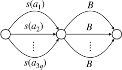
Figure 1: The reduction of $3$-Partition to MFD from [28]. The $3$-Partition instance consists of a set $A=\{a_{1},\dots,a_{3q}\}$, where every $a_{i}$ has a positive integer size $s(a_{i})$, and a positive integer $B$, such that $B/4<s(a_{i})<B/2$ holds for every $a_{i}\in A$. The question is whether $A$ can be partitioned into $q$ disjoint subsets, each of $3$ elements and of size $B$. The MFD series-parallel (see Definition 3.13) reduction consists of a subgraph obtained by the parallel composition of $3q$ edges with flow values $s(a_{1}),\dots,s(a_{3q})$, and a subgraph obtained by the parallel composition of $q$ edges, each with flow value $B$. These two graphs are composed with the series composition. Intuitively, because $B/4<s(a_{i})<B/2$ holds for every $a_{i}$, the MFD consists of exactly $3q$ paths of weights $s(a_{1}),\dots,s(a_{3q})$, and each edge on the right-hand subgraph is traversed by exactly three paths whose weights sum to $B$, giving thus the partition of $A$. Moreover, since the first $3q$ edges need to be decomposed, the previous decomposition is minimum even if negative weights are allowed, making MFD_Z NP-hard.

In Section 3 we study MFD_N ($0\in\mathbb{N}$), and in Section 4 we study MFD_Z and its generalisation MCCD_Z. Note that the reduction showing MFD_N to be strongly NP-hard from [28] also holds for MFD_Z (see Figure 1). However, a flow with non-negative values may admit a decomposition using fewer paths if negative weights are allowed, as shown in Figure 2. We explore further differences between MFD_N and MFD_Z in Sections 4 and 5.

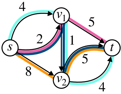
(a) If negative weights are allowed, the four paths decompose the flow with weights $4,5,8,$ and $-3$ (dark blue).

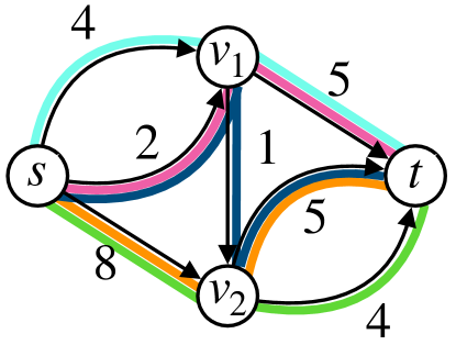
(b) With positive weights only, five paths are needed, since the edge $(v_{1},v_{2})$ must be decomposed by a weight $1$ path, leaving 4 edges that must be covered separately. The paths shown are one such decomposition.

Figure 2: A positive flow admitting a decomposition into four paths only if negative weights are allowed.

Let $\|X\|=\max_{(u,v)\in E}|X(u,v)|$ denote the infinity norm on flows or circulations. In particular, notice that if $\mathbb{Y}\subseteq\mathbb{Z}$, then $\|X\|\leq 1$ means that $X(u,v)\in\{0,\pm 1\}$ for every $(u,v)\in E$. Let $X\equiv_{2}Y$ iff $X$ and $Y$ have the same parity everywhere, i.e., for every $(u,v)\in E$, we have that $X(u,v)$ is odd iff $Y(u,v)$ is odd.

Definition 2.3.

Given $S\subseteq E$, we define $\textsf{width}_{S}(G)$ as the minimum number of $s$-$t$ paths in a DAG $G$ needed to cover all edges of $S$. If $S=E$ we just write $0pt{G}$.

The width is the main combinatorial tool that we use for our approximation results, and we will show in Section 3 that it is highly linked to the approximation performance of greedy-weight. Just like its more common node variant, $0pt{G}$ can be computed in $O(mn)$ time. As described by, e.g., [1, 5], this is done by reduction to a min-flow instance with demand one on every edge; the minimum flow of this instance is $0pt{G}$, and the flow can be found by reduction to a max-flow instance. Moreover, the problem can be relaxed to only require the coverage of $S\subseteq E$ and solved in the same running time by setting the demands only on the edges of $S$.

Lemma 2.4 ([1, 20]).

Let $G=(V,E)$ be a DAG, and $S\subseteq E$. A flow $C:E\to\mathbb{N}$ can be computed in $O(mn)$ time, such that $C(e)\geq 1$ for all $e\in S$ and $|C|=\textsf{width}_{S}(G)$.

The flow $C$ with total flow $\textsf{width}_{S}(G)$ suffices and we do not need to calculate a path cover achieving that minimum. However, we note that it can be directly computed given the flow $C$. We can think of this path cover as a flow decomposition of $C$ into $\textsf{width}_{S}(G)$ weight-one paths, which can be found by greedily removing such paths from $C$ until it is completely decomposed. Since each path has no more than $n-1$ edges and since $\textsf{width}_{S}(G)\leq m$, the overall runtime of finding the path cover is $O(mn)$. Similarly, every path cover $P_{1},\dots,P_{\ell}$ of $G$ defines a flow $C$ on $G$: $C=P_{1}+\dots+P_{\ell}$, and we say that $C$ is the induced flow of the path cover $(P_{i})_{i}^{\ell}$.

Definition 2.5.

In a directed graph $G=(V,E)$ we call a subset $C\subseteq E$ an antichain of $G$ if all edges in $C$ are pairwise parallel, that is there exists for no pair of edges in $C$ a path in $G$ leading from one edge to the other.

It can be shown with straight forward arguments that $0pt{G}=|C|$ for a maximum (sized) antichain $C$ of $G$.

3 Width matters for greedy approaches

Since the difference of two flows is still a flow, it is very natural to consider successively removing the simplest type of flow — that is to say, paths — as an algorithmic strategy for MFD_N. Indeed, the particular greedy path removal strategy of finding a heaviest path (greedy-weight) is commonly used as a heuristic in applications (e.g., [21, 2, 26, 14]) and it seems to be mentioned in nearly every paper addressing flow decomposition. More formally, a path $P$ is said to carry flow $p$ if $X(u,v)\geq p$ for all edges $(u,v)$ of $P$ (in particular, a $v$-$v$ path carries infinite flow). A heaviest path is an $s$-$t$ path carrying the largest flow. Such a path can be easily found in linear time in the size of the DAG by dynamic programming (see, e.g., [28]).

3.1 Width hinders greedy on MFD_N

We define a family of MFD_N instances $(G_{\ell},X_{\ell,B})$, depending on two parameters $\ell\in\mathbb{N}\setminus\{0\}$ and $B\in\mathbb{N}$. The family is defined recursively on $\ell$. The base case $(G_{1},X_{1,B})$ for $\ell=1$ is shown in Figure 3(a). For $\ell>1$, we build $(G_{\ell},X_{\ell,B})$ from two disjoint copies of $(G_{\ell-1},X_{\ell-1,B})$, by adding 5 extra edges and flow values as shown in Figure 3(b). We call the edge connecting the two copies of $G_{\ell-1}$ a central edge. Edges whose flow value depends on $B$ are called backbone edges, and they form a $s$-$t$ path. By choosing $B=2^{\ell+1}$, we show that the flow $X_{\ell,2^{\ell+1}}$ can be decomposed using a number of paths linear in $\ell$, thanks to the heavy backbone edges, whereas the greedy-weight algorithm fully saturates the central edges with its first path and is left with a remaining flow requiring $2^{\ell+1}$ paths to be decomposed.

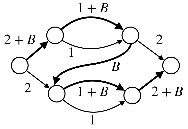
(a) The base case $(G_{1},X_{1,B})$ ($\ell=1$). Backbone edges (bold) carry $B$ flow.

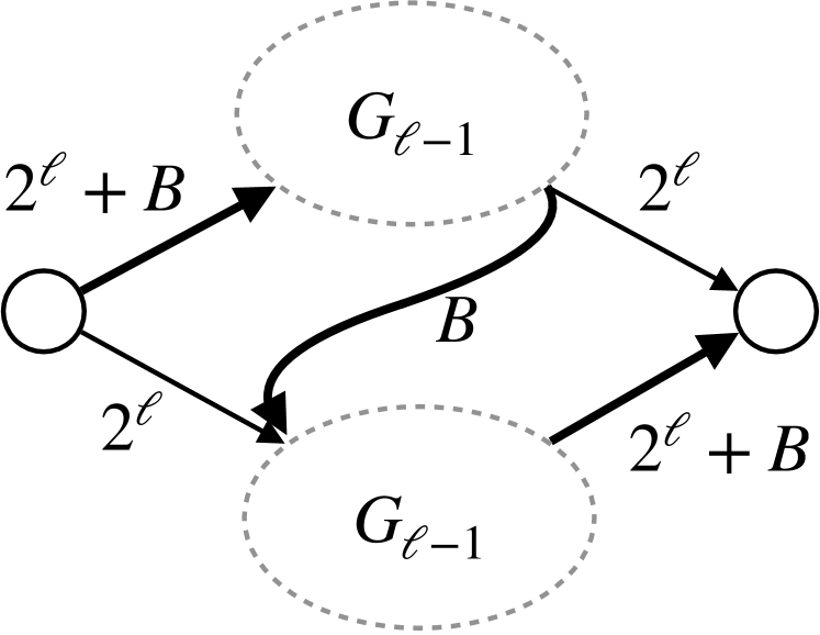
(b) Building $(G_{\ell},X_{\ell,B})$ from two copies of $(G_{\ell-1},X_{\ell-1,B})$ ($\ell>1$). The $5$ edges entering (resp. leaving) $(G_{\ell-1},X_{\ell-1,B})$ are defined to enter (resp. leave) the source (resp. sink) node of $(G_{\ell-1},X_{\ell-1,B})$. The central edge has flow $B$ and is part of the backbone (bold edges).

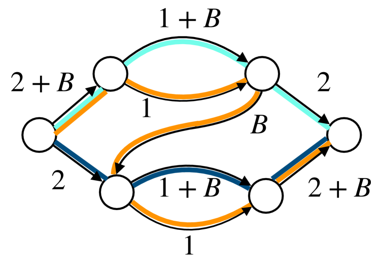
(c) Decomposing the base case $(G_{1},X_{1,B})$ ($\ell=1$), for $B=2^{\ell+1}$. All non-backbone edges can be decomposed with $2\ell+1=3$ paths. The orange path has weight $1$ and dark and light blue paths have weight $2$. A fourth path (of weight $3$) along the backbone is required to fully decompose the flow.

Figure 3: Construction for $(G_{\ell},X_{\ell,B})$. Setting $B=2^{\ell+1}$ yields MFD_N instances where greedy-weight uses $\Theta(\frac{m}{\log m})$ times more paths than optimal to decompose the flow.

Lemma 3.1.

Let $G_{\ell}$ with flow $X_{\ell,2^{\ell+1}}$ be constructed as described before. Greedy-weight uses $1+2^{\ell+1}$ paths to decompose $X_{\ell,2^{\ell+1}}$.

Proof 3.2.

We first show that the heaviest path in $X_{\ell,2^{\ell+1}}$ follows every backbone edge from $s$ to $t$. Certainly this path carries $2^{\ell+1}$ flow, and no more, since every backbone edge has flow at least $2^{\ell+1}$ and every central edge has flow exactly $2^{\ell+1}$. To see that there is no heavier path, observe that all the non-backbone edges have flow value strictly less than $2^{\ell+1}$ by construction. After removing that path with weight $2^{\ell+1}$, all the central edges are completely decomposed. The remaining graph and flow, without central edges, has $2^{\ell+1}$ weight-$1$ edges that are pairwise non-reachable using only non-zero flow edges (4 edges for each of the $2^{\ell-1}$ copies of $G_{1}$), each of which must be covered by a different path of weight $1$ (and these paths fully decompose the flow).

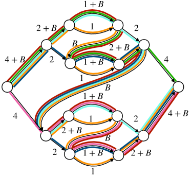
Figure 4: $(G_{2},X_{2,B=2^{\ell+1}})$ with a $2\ell+2=6$ flow decomposition. Orange (weight 1) and dark and light blue (weight 2) decompose the non-backbone edges in the two copies of $G_{1}$. Green and pink (weight 4) decompose the non-backbone edges added in $G_{2}$. Dark red (weight $3$) is the additional path needed to fully decompose the flow.

Lemma 3.3.

Let $G_{\ell}$ with flow $X_{\ell,2^{\ell+1}}$ be constructed as described before. It is possible to decompose $X_{\ell,2^{\ell+1}}$ using $2\ell+2$ paths.

Proof 3.4.

Using induction, we first prove that we can use $2\ell+1$ paths to decompose all of the flow of $X_{\ell,2^{\ell+1}}$ on the non-backbone edges of $G_{\ell}$, and that these paths have total weight $2^{\ell+2}-3$. When $\ell=1$ (see Figure 3(c)), we can decompose both the flow-$1$ edges with a single path of weight $1$ which goes through the central edge. Moreover, we can decompose the flow-$2$ edges with two paths of weight $2$, without using the central edge. These paths have $5=2^{1+2}-3$ total flow. We now assume that the claims hold for $\ell=k$ and prove it for $\ell=k+1$. Consider the graph $G_{k+1}$. By assumption, the non-backbone edges in every copy of $G_{k}$ are fully decomposed by $2k+1$ paths, and the total flow of those paths is $2^{k+2}-3$. Note that these paths are $s$-$t$ paths in $G_{k}$, but they must be extended to be $s$-$t$ paths in $G_{k+1}$. Because there is a central edge with weight $2^{(k+1)+1}=2^{k+2}>2^{k+2}-3$ from one copy of $G_{k}$ to the other, it is possible to route the $2k+1$ paths from the first $G_{k}$ to the second using the central edge. Additionally, the backbone edges from $s$ to the first copy of $G_{k}$ and from the second copy of $G_{k}$ to $t$ have flow $2^{k+1}+2^{k+2}$, so they can be used to complete the routing of the paths from $s$ to $t$. Then we can use two additional paths of weight $2^{k+1}$ each to decompose the flow of the two new non-backbone edges; one using the backbone path of the upper $G_{k}$ (extended by the upper edges of $G_{k+1}$), and analogously, the other through the backbone path of the lower $G_{k}$, which is possible since the paths obtained inductively only decompose $2^{k+1}$ of the backbone flow of $G_{k}$ whereas now $2^{k+2}$ backbone flow must be decomposed. As such, we use $2k+1+2=2(k+1)+1$ paths with total flow $2^{k+2}-3+2(2^{k+1})=2^{(k+1)+2}-3$, as required. By the previous, given any graph $G_{\ell}$, we can decompose all non-backbone edges using $2\ell+1$ paths. Note that removing these weighted paths from $X_{\ell,2^{\ell+1}}$ yields a flow on $G_{\ell}$ (of value $3$). Because the remaining edges (all backbone) form a path from $s$ to $t$, and the remaining edge values form a flow on $G_{\ell}$, all remaining edges must have the same flow value, and can be covered by one path. Thus, $2\ell+2$ paths are sufficient to decompose $X_{\ell,2^{\ell+1}}$. See Figure 4 for an example when $\ell=2$.

See 1.1

Proof 3.5.

By Lemmas 3.1 and 3.3, greedy-weight uses $\Theta(2^{\ell})$ paths to decompose the flow $X_{\ell,2^{\ell+1}}$ described above, whereas it is possible to decompose the flow with only $\Theta(\ell)$ paths. It can be easily verified by induction that the number of edges of $G_{\ell}$ is $7\cdot 2^{\ell}-5$. So the ratio between greedy-weight and the optimal for this instance is $\Omega(\frac{m}{\log m})$.

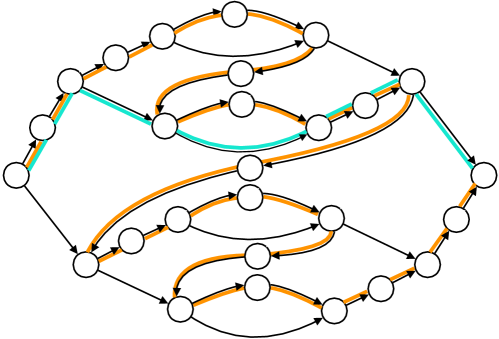
Figure 5: By subdividing the backbone edges, choosing longest paths (orange) and shortest paths (blue) both give the same approximation ratio as choosing heaviest paths in the original flow $X_{\ell,2^{\ell+1}}$.

While greedy-weight is most commonly used in applications, the approach was first presented as part of a general framework [28]: pick any optimality criteria for $s$-$t$ paths that is saturating (i.e., fully decomposes at least one edge), and successively remove optimal paths. Since each path is saturating, the algorithm must decompose the flow in $m$ or fewer paths. Another optimality criterion sometimes used in DNA assembly (e.g., in vg-flow [2]) is the longest path (with its maximum possible flow so that it is saturating). To adapt our construction of $(G_{\ell},X_{\ell,2^{\ell+1}})$ so that this approach yields the same approximation ratio, consider $(G_{\ell}^{*},X_{\ell,2^{\ell+1}}^{*})$, constructed as in $(G_{\ell},X_{\ell,2^{\ell+1}})$ except that we split every backbone edge $(u,v)$ into two edges, $(u,w)$ and $(w,v)$. See Figure 5 for an example. Then the path along the backbone edges will be the longest from $s$ to $t$ and the previous asymptotic analysis still holds, since we no more than doubled the number of edges (and the number of edges of the new construction is still $\Theta(2^{\ell})$). Yet another optimality criterion, studied in [14] for its application to network routing, is the shortest path (again with its maximum possible flow). $(G_{\ell}^{*}$, $X_{\ell,2^{\ell+1}}^{*})$ will also force this approach to take an exponential number of paths, since first the algorithm will decompose all $2^{\ell+1}$ weight-$1$ edges with $2^{\ell+1}$ different paths.

3.2 Greedy approximation for width-stable graphs

As exploited in Section 3.1, one sticking point for greedy path removal algorithms is the fact that the width of a graph can increase after an edge is fully decomposed. We now identify a new class of graphs, in which the graph does not increase its width during the execution of the algorithm. We show that greedy-weight decomposes “enough” flow at each step in these graphs, giving a $O(\log|X|)$-approximation for MFD_N.

If $X\geq 0$ is a flow on a DAG $G$, we write $G|_{X}$ ($G$ restricted to $X$) to mean the spanning subgraph of $G$ made up of the edges $e\in E$ such that $X(e)\neq 0$. Conversely, if $S$ is a subgraph of $G$, we write $X|_{S}$ ($X$ restricted to $S$) to mean the pseudo-flow $X$ only on the edges of $S$. In the case of MFD_N, once an edge is fully decomposed, it cannot be used in future paths, possibly increasing the width of the graph that can be used to decompose the rest of the flow and sometimes triggering an increase of the size of a minimum flow decomposition as well. We call a graph width-stable if it does not have this issue.

Definition 3.6 (Width-stable graph).

We say that a graph $G$ is width-stable if, for any non-negative flows $X\leq Y$ on $G$, it holds that $0pt{G|_{X}}\leq 0pt{G|_{Y}}$.

Many useful MFD_N instances satisfy Definition 3.6. For example, the first proof of MFD’s NP-hardness [28] was a reduction to a very simple graph of this form, as shown in Figure 1; this means that MFD_N restricted to width-stable graphs is also NP-hard.

Definition 3.7 ([12]).

We call an $s$-$t$ DAG $G$ funnel if every $s$-$t$ path has a private edge that is not contained in any other $s$-$t$ path.

Funnels are simple graphs in the sense that they admit a unique flow decomposition [16]. We use funnels in Lemma 3.8 to characterize graphs that are not width-stable. Funnels generalise in/out-forests: along any $s$-$t$ path nodes $v$ first satisfy $\deg^{-}(v)\leq 1\leq\deg^{+}(v)$ and then $\deg^{-}(v)\geq 1\geq\deg^{+}(v)$. We call a node $v$ forking (resp. merging) if $\deg^{+}(v)>1$ (resp. if it is $\deg^{-}(v)>1$). For a funnel subgraph $F$ of $G$ we call a path in $G$ from a merging node in $F$ to a forking node in $F$ a central path of the funnel. The graphs $(G_{\ell},X_{\ell,B})$ in Section 3.1 are precisely funnels with central paths.

The next property that we need is that there is always, during the execution of the greedy-weight algorithm, a path carrying “enough” flow from $s$ to $t$.

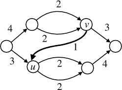
Figure 6: MFD_N instance with $0pt{G}=3$, $|X|=7$, $|X|/0pt{G}=7/3>2$, but no path can carry more flow than $2$. By Lemma 3.8, this is equivalent to $G$ not being width-stable, there exists an $s$-$t$ path saturating the central edge from $v$ to $u$ of weight $1$, making the graph a funnel and increasing $0pt{G}$ to $4$.

Lemma 3.8.

Let $G$ be an $s$-$t$ DAG. The following statements are equivalent:

1. $G$ is width-stable,

2. $G$ has paths of large weight: for any flow $X\geq 0$ on $G$, there exists an $s$-$t$ path in $G|_{X}$ carrying $|X|/0pt{G|_{X}}$ flow,

3. $G$ has no funnel subgraph with a central path.

See Figure 6 for an example.

Proof 3.9.

$(\ref{lem:enough-flow-stable})\implies(\ref{prop:enough-flow})$: Let $G=(V,E)$ be an $s$-$t$ DAG with flow $X\geq 0$ for which there is no $s$-$t$ path in $G|_{X}$ carrying $b=|X|/0pt{G|_{X}}$ flow. We will show that $G$ is not width-stable. For simplicity, we assume $G=G|_{X}$, the result follows immediately for any supergraph of $G$. Let $S$ be the set of vertices reachable from $s$ by a path carrying $b$ flow. By assumption, $t\notin S$, so $(S,V\setminus S)$ is an $s,t$-cut and $X(u,v)<b$ for any edge $(u,v)$ with $u\in S,v\in V\setminus S$. Define $T$ to be the set of vertices that can reach $t$ via a path involving vertices only from $V\setminus S$:

$$T\coloneqq V\setminus\{v\in V\mid\text{all $v-t$ paths cross $S$}\}.$$

Since $S\subseteq V\setminus T$, $(V\setminus T,T)$ is an $s,t$-cut. Note that if $(u,v)$ is an edge with $u\in V\setminus T$ and $v\in T$, then also $u\in S$ and $v\in V\setminus S$ and thus $X(u,v)<b$. The set $C$ defined by

$$C\coloneqq\{(u,v)\in E\mid u\in V\setminus T,v\in T\}=E\cap(S\times T)$$

is an $s,t$-cut set (a set of edges that every $s$-$t$ path has to cross) and we have $X(e)<b$ for every $e\in C$. This implies $|C|>0pt{G}$.

We construct a new flow $Y\geq 0$ on $G$ for which $C$ is an antichain in $G|_{Y}$. Initially, $Y\coloneqq X$. Define the following paths:

• $p_{s}(u)$ for all $u\in S$: an $s$-$u$ path with all nodes in $S$,

• $p_{t}(v)$ for all $v\in T$: a $v$-$t$ path with all nodes in $T$.

We keep the invariant that the paths exist and do not change in $G|_{Y}$ throughout the construction of $Y$. Let denote a path from $v\in T$ to $u\in S$, all of whose internal nodes are from $V\setminus(S\cup T)$, as $b(v,u)$, and note that such a path exists iff $C$ is not an antichain. Assume it carries flow $\mu>0$ (i.e., $\mu$ is the minimum flow along $b(v,u)$), we then perform the following operation on $Y$:

$$Y(e)=\begin{cases}Y(e)-\mu&\text{if }e\in b(v,u)\\ Y(e)+\mu&\text{if }e\in p_{s}(u)\cup p_{t}(v).\end{cases}$$

Note that after the operation $Y$ remains a flow and that none of the three paths have pairwise intersecting edges. The process does not violate the invariant and repeating eventually it destroys all paths from $T$ to $S$, making $C$ an antichain in $G|_{Y}$. This shows that $G$ is not width-stable: $Y\leq X+Y$ and $0pt{G|_{Y}}>0pt{G|_{X+Y}}=0pt{G}$.

$(\ref{prop:enough-flow})\implies(\ref{lem:enough-flow-no-backbone})$: Assume that $G$ has a funnel subgraph $F$ with a central path $P$. Let $C$ be a maximum antichain of $F$, and note that every maximum antichain of a funnel consists of private edges only. We define flows $Z_{\text{stable}}$, $Z_{unstable}$ and $Z$:

• $Z_{\text{stable}}$ is defined to be the flow induced by the minimum path cover of $F$ (i.e., $G|_{Z_{\text{stable}}}=F$).

• $Z_{\text{unstable}}$ is defined to be the flow induced by the following path cover of the graph consisting of $F$ and $P$: One $s$-$t$ path goes along $P$, covering two edges in $C$, and the other paths cover $F$ avoiding $P$, this is possible with additional $|C|-2$ paths.

• Finally, $Z\coloneqq Z_{\text{stable}}+Z_{\text{unstable}}$.

We have $|Z|=|Z_{\text{stable}}|+|Z_{\text{unstable}}|=|C|+(|C|-1)=2|C|-1$ and $0pt{G|_{Z}}\leq|C|-1$, and thus

$$\frac{|Z|}{0pt{G|_{Z}}}\geq\frac{2|C|-1}{|C|-1}>2,$$

but all $s$-$t$ paths in $G$ carry no more flow than $2$, because $C$ is an $s,t$-cut set of $G$ and all $Z$ flow values on $C$ are $2$.

$(\ref{lem:enough-flow-no-backbone})\implies(\ref{lem:enough-flow-stable})$: Assume that $G=(V,E)$ is not width-stable, let $Y\geq X\geq 0$ be flows on $G$ with $0pt{G|_{X}}>0pt{G|_{Y}}$ and let $C^{\prime}$ be a maximum antichain of $G|_{X}$. Let $F$ be a funnel subgraph of $G|_{X}$ containing $C^{\prime}$ as maximum antichain, and let $C$ be the rightmost maximum antichain of $F$ (that is, the head of every edge in $C$ is $t$ or is merging). Since $C$ is not an antichain of $G|_{Y}$, there must be a path $P$ in $G|_{Y}$ connecting two edges in $C$, and it starts at a merging node. It must also enter a forking node, because otherwise adding the path would not decrease the width. This shows that a prefix path of $P$ is a central path of $F$.

Lemma 3.10.

Let $G=(V,E)$ be a width-stable graph, $0pt{G}\geq 2$. Greedy-weight uses at most $\lfloor\log|X|/\log\frac{0pt{G}}{0pt{G}-1}\rfloor+1$ paths to decompose any flow $X:E\to\mathbb{N}$.

Proof 3.11.

Let $b=0pt{G}$. Since $G$ is width-stable, greedy-weight removes a path of weight at least $|X^{\prime}|/b$ at every step by Lemma 3.8, where $X^{\prime}$ is the remaining flow of the corresponding step. As such, after $c$ steps $|X^{\prime}|\leq|X|\left(\frac{b-1}{b}\right)^{c}$. If $|X|\left(\frac{b-1}{b}\right)^{c}<1$, then $|X^{\prime}|=0$, since $|X|$ and the weights of the removed paths belong to $\mathbb{N}$. Solving for $c$ we obtain $c>\log|X|/\log\frac{b}{b-1}$. Therefore, greedy-weight takes (uses) at most $c=\lfloor\log|X|/\log\frac{b}{b-1}\rfloor+1$ steps (paths).

See 1.2

Proof 3.12.

Assume $X>0$ (otherwise, replace $G$ by $G|_{X}$). Thus, $b=0pt{G}\leq\textsf{mfd}_{\mathbb{N}}(G,X)$, since any flow-decomposition of $X$ induces a path cover of $E$. If $b\leq 1$ greedy-weight finds an optimal solution. Otherwise $b\geq 2$, and Lemma 3.10 implies that greedy-weight is a $O(\frac{\log|X|}{b\log\frac{b}{b-1}})=$$O(\log|X|)$-approximation for MFD_N ($b\log\frac{b}{b-1}=O(1)$ for $b\geq 2$).

Finally, we show that series-parallel graphs are width-stable, and thus greedy-weight is a $O(\log{|X|})$-approximation on them.

Definition 3.13 (Series-parallel graph [9]).

A graph is a two-terminal series-parallel (series-parallel for short) graph with terminal nodes $s$ and $t$ if:

• it consists of a single edge directed from $s$ to $t$, and no other nodes, or

• it can be obtained from two (smaller) two-terminal series-parallel graphs $G_{1}$ and $G_{2}$, with terminal nodes $s_{1},t_{1}$, and $s_{2},t_{2}$, respectively, by either

  • identifying $s=s_{1}=s_{2}$ and $t=t_{1}=t_{2}$ (parallel composition of $G_{1}$ and $G_{2}$), or

  • identifying $s=s_{1}$, $t_{1}=s_{2}$, and $t=t_{2}$ (series composition of $G_{1}$ and $G_{2}$).

Corollary 3.14.

Greedy-weight is a $O(\log|X|)$-approximation for MFD_N on series-parallel graphs.

Proof 3.15.

Using Theorem 1.2, it remains to prove that any series-parallel graph $G=(V,E)$ with any flow $X:E\to\mathbb{N}$ is width-stable. We prove it using structural induction. The base case is when $G$ is single edge from $s$ to $t$, and they are trivially width-stable.

Suppose now that $G$ is obtained by the composition of series-parallel graphs $G_{1},G_{2}$, and let $X\leq Y$ by any non-negative flows on $G$. Let $X_{i}=X|_{G_{i}},Y_{i}=Y|_{G_{i}}$ and let $x_{i}$ denote $0pt{G_{i}|_{X_{i}}}$, $y_{i}$ denote $0pt{G_{i}|_{Y_{i}}}$, for $i=1,2$. $x_{i}\leq y_{i}$ for $i=1,2$.

If the composition operation is parallel composition, then $0pt{G}=0pt{G_{1}}+0pt{G_{2}}$ (since edges of $G_{1}$ cannot reach edges of $G_{2}$, and vice versa) and $0pt{G|_{X}}=x_{1}+x_{2}$, $0pt{G|_{Y}}=y_{1}+y_{2}$ (since $G|_{X}$ and $G|_{Y}$ are also series-parallel), and $G$ is width-stable by the inductive hypothesis that $x_{i}\leq y_{i}$, for $i=1,2$.

If the composition operation is series composition, width-stability follows analogously to the parallel composition by replacing sum with maximum.

However, note that there are width-stable graphs that are not series-parallel.

4 Width helps solve MCCD_Z

In this section we give an approximation algorithm for $\textsf{mfd}_{\mathbb{Z}}(G,X)$. We will obtain this for a more general problem variant, which can be defined as follows. We are given directed a graph $G=(V,E,c)$ with no sink or source nodes, with (cost) a function $c:E\to\mathbb{R}_{\geq 0}$. The cost of a circulation $X$ is defined as $\tilde{c}(X)=\sum_{e\in E}c(e)X(e)$. Note that $\tilde{c}(\cdot)$ is a linear function: $\tilde{c}(X+Y)=\tilde{c}(X)+\tilde{c}(Y)$ for any two circulations $X,Y$ on $G$.

Definition 4.1.

Given $(G,X)$ of a graph $G=(V,E,c)$ and a circulation $X:E\to\mathbb{Y}$, a circulation decomposition of size $k$ of $(G,X)$ is a family of circulations $Y_{i}:E\to\mathbb{N}$ with weights $(w_{1},\dots,w_{k})\in\mathbb{Y}^{k}$ such that $X=w_{1}Y_{1}+\dots+w_{k}Y_{k}$. We call the problem of finding a circulation decomposition of minimum cost $\tilde{c}(Y_{1}+\dots+Y_{k})$ the Minimum Cost Circulation Decomposition or MCCD_Y and we write $\textsf{mccd}_{\mathbb{Y}}(G,X)$ for the minimum cost.

Decomposing into non-negative weighted circulations rather than paths is a natural generalisation, as paths can also be seen as flows with value $1$ along the path. The following reduction (Figure 7) shows that MFD_Y can be regarded as a special case of MCCD_Y.

Lemma 4.2.

MCCD_Y is NP-hard.

Proof 4.3.

Given an $s$-$t$ DAG $G=(V,E)$ and flow $X:E\to\mathbb{Y}$, we define a graph $G^{\prime}=(V,E^{\prime},c)$ with $E^{\prime}=E\cup\{(t,s)\}$ and $c:E^{\prime}\to\{0,1\}$, $c(u,v)=1\iff(u,v)=(t,s)$, i.e. cost $1$ only for the edge $(t,s)$. Let $X^{\prime}:E^{\prime}\to\mathbb{Y},X^{\prime}(e)=X(e)$ for $e\in E$ and $X^{\prime}(t,s)=|X|$ be a circulation on $G^{\prime}$. The cost of a Minimum Cost Circulation Decomposition $(Y^{\prime}_{1},w^{\prime}_{1}),\dots,(Y^{\prime}_{k},w^{\prime}_{k})$ of $(G^{\prime},X^{\prime})$ is equal to $\tilde{c}(Y^{\prime}_{1})+\dots+\tilde{c}(Y^{\prime}_{k})=Y^{\prime}_{1}(t,s)+\dots+Y^{\prime}_{k}(t,s)$. Note that an $s$-$t$ path $P:E\to\{0,1\}$ yields a circulation $Y_{P}:E^{\prime}\to\{0,1\}$ of cost $1$, which implies $\textsf{mfd}_{\mathbb{Y}}(G,X)\geq\textsf{mccd}_{\mathbb{Y}}(G^{\prime},X^{\prime})$. Define flows $Y_{i}:E\to\mathbb{Y}$ with $Y_{i}(e)=Y^{\prime}_{i}(e)$ for $i=1,\dots,k$. Decomposing each flow $Y_{i}$ trivially into $|Y_{i}|=Y^{\prime}_{i}(t,s)$ paths and assigning them weights $w^{\prime}_{i}$ yields a Flow Decomposition of $(G,X)$, showing $\textsf{mccd}_{\mathbb{Y}}(G^{\prime},X^{\prime})\geq\textsf{mfd}_{\mathbb{Y}}(G,X)$, and thus this Flow Decomposition is minimum.

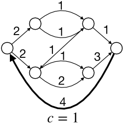
Figure 7: Reduction in Lemma 4.2 of a graph with total flow $4$ from MFD_Y to MCCD_Y. The bold edge is the addition to the DAG and is the only edge with cost $1$ while all other edges have cost $0$.

Definition 4.4.

Given $S\subseteq E$ and a graph $G$, we call a circulation $C$ of minimum cost satisfying $C(e)\geq 1$ for all $e\in S$ Minimum Cost Circulation Cover of $S$, and we write $\textsf{mccc}_{S}(G)=\tilde{c}(C)$. If $S=E$, we use $\textsf{mccc}(G)$ instead.

Note that since every circulation decomposition of a graph $G$ covers the edges of non-zero circulation, $\textsf{mccc}_{S}(G)\leq\textsf{mccd}_{\mathbb{Y}}(G,X)$ with $S=\{e\in E\mid X(e)\neq 0\}$. This generalises the width lower bound of MFD_Y to MCCD_Y. Given an $s$-$t$ DAG $G$, $0pt{G}=\textsf{mccc}(G^{\prime})$ for the graph $G^{\prime}$ obtained by the reduction in Lemma 4.2. We will need a Minimum Cost Circulation Cover for our approximation approach:

Lemma 4.5 ([11], Theorem 3.6).

Let $G=(V,E,c)$ be a graph, and $S\subseteq E$. A Minimum Cost Circulation Cover of $S$ can be computed in $O(n\log m(m+n\log n))$ time.

The idea behind our approximation algorithm for MCCD_Z is that a circulation $X:E\to\mathbb{Z}$ on a graph $G$ can always be decomposed into circulations of total cost $(\lceil\log\|X\|\rceil+1)\cdot\textsf{mccc}(G)$. We show this using two key facts: first, that $X$ can be decomposed into $(\lceil\log\|X\|\rceil+1)$ circulations with a particular structure, and, second, that each of these circulations can be further decomposed into circulations of total cost of at most $\textsf{mccc}(G)$. A key step in proving both these facts is a subroutine which, given an input circulation $X$, finds another circulation $Y$ with values from $\{0,\pm 1\}$ only (a unitary circulation) that matches the parity of $X$ on all edges. Intuitively, given an input circulation $X$, such a unitary circulation $Y$ can be added to $X$ to “fix” its odd edges to be even, with only a small change to $X$.

Lemma 4.6.

For any circulation $X:E\to\mathbb{Z}$ on $G=(V,E,c)$, there exists a circulation $Y:E\to\mathbb{Z}$ such that $X\equiv_{2}Y$ and $\|Y\|\leq 1$.

Proof 4.7.

Consider the undirected graph $G_{\mathrm{odd}}=(V,E_{\mathrm{odd}})$ where $E_{\mathrm{odd}}=\{\{u,v\}\mid(u,v)\in E\text{ and }X(u,v)\text{ is odd}\}$.

Notice that every node of $G_{\mathrm{odd}}$ has even degree due to the conservation of circulation. Thus, $G_{\mathrm{odd}}$ can be written as the edge-disjoint union of cycles. Assign an arbitrary orientation to each cycle and let $E_{\mathrm{odd}}^{+}$ be the set of edges oriented in this way. Define

$$Y(u,v)=\begin{cases}+1&\text{if }(u,v)\in E_{\mathrm{odd}}^{+}\\ -1&\text{if }(v,u)\in E_{\mathrm{odd}}^{+}\\ 0&\text{if }\{u,v\}\notin E_{\mathrm{odd}}\end{cases}$$

Notice that $Y$ is a circulation decomposed as a sum of circulations, each along one of the edge-disjoint cycles. Moreover, $X\equiv_{2}Y$ and $\|Y\|\leq 1$ by construction.

Repeatedly applying Lemma 4.6 and dividing the resulting even circulation by 2, we obtain the the first key ingredient of the approach.

Corollary 4.8.

Any (non-zero) circulation $X:E\to\mathbb{Z}$ can be written as $X=\sum_{i=0}^{\lceil\log\|X\|\rceil}2^{i}\cdot Y_{i}$, where $Y_{i}:E\to\mathbb{Z}$ is a circulation with $\|Y_{i}\|\leq 1$ for all $i$.

Proof 4.9.

If $||X||\leq 1$ the result follows. Otherwise apply Lemma 4.6 to obtain $Y_{0}$ such that $X\equiv_{2}Y$ and $\|Y_{0}\|\leq 1$. Since $X\equiv_{2}Y_{0}$, we can define $X^{\prime}=(X-Y_{0})/2$, and thus $X=2X^{\prime}+Y_{0}$. Recursively repeat this procedure on $X^{\prime}$ until $||X^{\prime}||\leq 1$, obtaining $Y_{0},\ldots,Y_{k}=X^{\prime}$, so that $X=\sum_{i=0}^{k}2^{i}\cdot Y_{i}$. Finally, note that at each repetition, $||X||$ decreases to at most $\lceil||X||/2\rceil$, thus $k\leq\lceil\log{||X||}\rceil$.

The following result is the second key ingredient of our approach. It guarantees that any unitary circulation can be decomposed into two circulations of total cost of at most $\textsf{mccc}(G)$ (see Figure 8 for an example). This is by no means obvious since, among other problems, a unitary circulation may contain positive and negative values which merge and cancel each other out (as in Figure 8(b)).

Lemma 4.10.

For any circulation $X:E\to\mathbb{Z}$, $\|X\|\leq 1$, there exist circulations $A,B:E\to\mathbb{Z}$ such that:

1. $A,B\geq 0$

2. $X=A-B$

3. $\tilde{c}(A)+\tilde{c}(B)\leq\textsf{mccc}(G)$

Proof 4.11.

Take $C$ such that $C\geq 1$ and $\tilde{c}(C)=\textsf{mccc}(G)$, according to Lemma 4.5. Take $D$ such that $D\equiv_{2}X+C$ and $\|D\|\leq 1$, according to Lemma 4.6. Also, assume $\tilde{c}(D)\geq 0$ without loss of generality (otherwise, take $-D$, which satisfies the same properties).

Since $D\equiv_{2}X+C$, we have $C-D\pm X\equiv_{2}0$. So we can take $A=(C-D+X)/2$ and $B=(C-D-X)/2$.

1. Notice that $C-D\pm X\geq C-2$ since $\|D\|,\|X\|\leq 1$. So, $C-D\pm X\geq-1$, since $C\geq 1$. But $C-D\pm X\equiv_{2}0$ so $C-D\pm X\geq 0$, whence $A,B\geq 0$.

2. $A-B=\frac{C-D+X}{2}-\frac{C-D-X}{2}=X$.

3. $\tilde{c}(A)+\tilde{c}(B)=\tilde{c}(A+B)=\tilde{c}(\frac{C-D+X}{2}+\frac{C-D-X}{2})=\tilde{c}(C-D)=\tilde{c}(C)-\tilde{c}(D)\leq\tilde{c}(C)$ since $\tilde{c}(D)\geq 0$, and $\tilde{c}(C)=\textsf{mccc}(G)$.

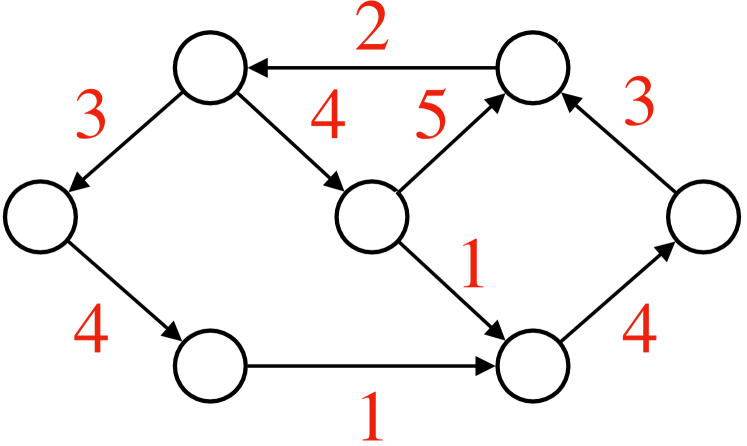
(a) Edge costs

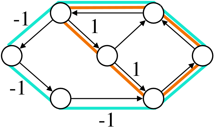
(b) Unitary circulation $X$ on a graph $G$ and a decomposition into two non-negative circulations $A$ and $B$, of weight $1$ in orange (see (e)), and of weight $-1$ in blue (see (f)), respectively.

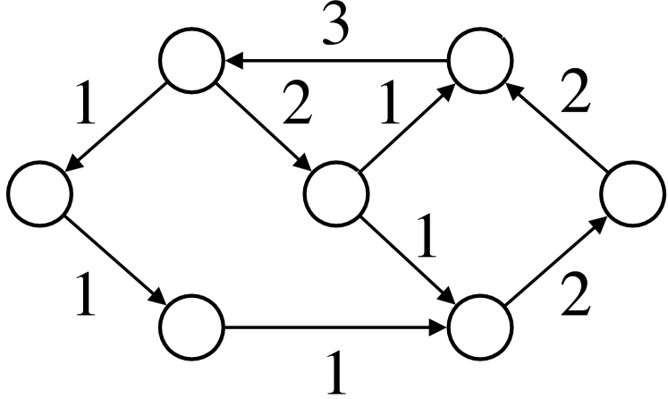
(c) Circulation $C$ covering all edges of $G$, of cost $\tilde{c}(C)=\textsf{mccc}(G)=42$ (Lemma 4.5).

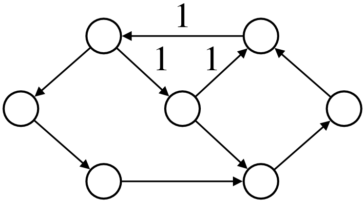
(d) Unitary circulation $D$ of cost $11$ matching the parity of $X+C$, i.e., $D\equiv_{2}X+C$ (Lemma 4.6).

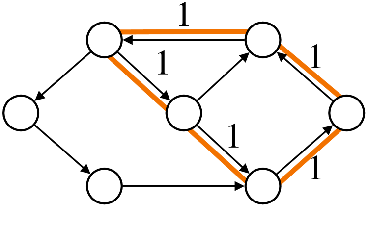
(e) Circulation $A=(C-D+X)/2$ of cost $14$.

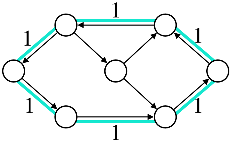
(f) Circulation $B=(C-D-X)/2$ of cost $17$.

Figure 8: Example of Lemma 4.10 applied to a unitary circulation $X$ on a graph $G$ (for clarity, $0$ circulation values are not shown). Non-negative circulations $A$ and $B$ can be constructed so that $\tilde{c}(A)+\tilde{c}(B)\leq\textsf{mccc}(G)$ holds. We obtain a decomposition of $X$ by $X=A-B$.

Finally, expressing any circulation as a sum of at most $\lceil\log\|X\|\rceil+1$ unitary circulations (Corollary 4.8), and decomposing each unitary circulation into two circulations with cost of at most $\textsf{mccc}(G)$ (Lemma 4.10), we can decompose the circulation into circulations of total cost no more than $\lceil\log\|X\|\rceil+1$ whose weights are positive and negative powers of two.

Theorem 4.12.

Given a graph $G=(V,E,c)$ and a circulation $X\colon E\to\mathbb{Z}$ with $k\coloneqq\lceil\log\|X\|\rceil$, there exist circulations $A_{i},B_{i}$ for $i=0,\dots,k$ and weights $\{w_{0},\dots,w_{k}\}\subseteq\{2^{i}\leavevmode\nobreak\ |\leavevmode\nobreak\ i\in\mathbb{N}\}$, with $\tilde{c}(A_{0}+\dots+A_{k}+B_{0}+\dots+B_{k})\leq(k+1)\cdot\textsf{mccc}(G)$ such that $X=w_{0}(A_{0}-B_{0})+\dots+w_{k}(A_{k}-B_{k})$.

Proof 4.13.

Combine Corollary 4.8 and Lemma 4.10, getting

$$X =\sum_{i=0}^{k}2^{i}\cdot Y_{i}=\sum_{i=0}^{k}2^{i}\cdot(A_{i}-B_{i})$$

where $\tilde{c}(A_{i}+B_{i})\leq\textsf{mccc}(G)$.

The proof of Theorem 4.12 suggests a straightforward algorithm for MCCD_Z, which we detail in Algorithm 2 and describe at a high level here. First, iteratively decompose $X$, yielding $\log\lceil\|X\|\rceil+1$ unitary circulations. Then use Lemma 4.10 to decompose each into two circulations of cost at most $\textsf{mccc}(G)$. However, $\textsf{mccc}(G)$ is not necessarily a lower bound on MCCD_Z if the circulation is $0$ on some edges, and thus this approach does not directly derive an approximation. To overcome this issue, we instead find a circulation decomposition of a spanning subgraph $G^{\prime}$ of $G$ for which $\textsf{mccc}(G^{\prime})$ lower bounds $\textsf{mccd}_{\mathbb{Z}}(G,X)$. Namely, we first find a minimum cost circulation cover in $G$ of the subset $S$ of edges with non-zero flow in $O(n\log m(m+n\log n))$ time (according to Lemma 4.5), and then remove from $G$ any edge not covered by the circulation, obtaining $G^{\prime}$. By construction, the cost of this circulation cover is a lower bound of $\textsf{mccd}_{\mathbb{Z}}(G,X)$. Moreover, the cost of this circulation cover is exactly $\textsf{mccc}(G^{\prime})$, since every circulation cover of $G^{\prime}$ is also a circulation cover of $S$ in $G$.

To prove the correctness of Algorithm 2, we first define a a subroutine implementing Lemma 4.6.

Lemma 4.14.

Algorithm 1 returns a unitary circulation from an input circulation $Y$ such that $X\equiv_{2}Y$, as in Lemma 4.6, in $O(m)$ time.

Proof 4.15.

The correctness of the algorithm is given by Lemma 4.6. Finally, the first $3$ subroutines as well as the entire for-loop takes $O(m)$ time.

Algorithm 1 Unitary(G,X): Produces a unitary circulation $Y$ from an input circulation $X$ such that $X\equiv_{2}Y$, as in Lemma 4.6

1:  $E_{odd}\leftarrow$ odd edges of G, undirected

2:  $C\leftarrow$ a decomposition of $G_{odd}=(V,E_{odd})$ into cycles, oriented arbitrarily

3:  $E_{odd}^{+}\leftarrow$ directed edges of C

4:  for $(u,v)\in E$ do

5:     if $(u,v)\in E_{odd}^{+}$ then

6:        $Y(u,v)\leftarrow+1$

7:     else if $(v,u)\in E_{odd}^{+}$ then

8:        $Y(u,v)\leftarrow-1$

9:     else

10:        $Y(u,v)\leftarrow 0$

11:     end if

12:  end for

13:  return Y

Algorithm 2 Finds the circulation decomposition of Theorem 4.12

1:  Compute a minimum cost circulation cover of $\{(u,v)\in E\mid X(u,v)\neq 0\}$ {Lemma 4.5}

2:  Remove from $G$ any edge not covered by this circulation cover to obtain $G^{\prime}$

3:  $\mathcal{P}\leftarrow[]$, $\mathcal{W}\leftarrow[]$ {length-zero vectors}

4:  $C\leftarrow$ circulation of cost $\textsf{mccc}(G^{\prime})$, $C\geq 1$ {Lemma 4.5}

5:  $D\leftarrow\textsc{Unitary}(G^{\prime},C)$; if $|D|<0$ set $D=-D${Algorithm 1}

6:  $i\leftarrow 0$

7:  while $\|X\|>1$ do

8:     $Y_{i}\leftarrow\textsc{Unitary}(G^{\prime},X)${Algorithm 1}

9:     $X\leftarrow(X-Y_{i})/2$

10:     $i\leftarrow i+1$

11:  end while

12:  $Y_{i}\leftarrow X$

13:  for $j\in\{0,\ldots,i\}$ s.t. $Y_{j}\neq 0$ do

14:     $A\leftarrow C-D+Y_{j}$, $B\leftarrow C-D-Y_{j}$

15:     Concatenate $A$ and $B$ to $\mathcal{P}$

16:     Concatenate $2^{j}$ and $-2^{j}$ to $\mathcal{W}$

17:  end for

18:  return $(\mathcal{P},\mathcal{W})$

See 1.3

Proof 4.16.

By Theorem 4.12 and our previous discussion, Algorithm 2 returns a circulation decomposition for $X$ with no more cost than $(\lceil\log\|X\|\rceil)+1\cdot\textsf{mccc}(G^{\prime})\leq(\lceil\log\|X\|\rceil+1)\cdot\textsf{mccd}_{\mathbb{Z}}(G,X)$. We analyse the runtime line by line. Lines 1 and 4 take $O(n\log m(m+n\log n))$ time by Lemma 4.5. The call to Algorithm 1 on line 5 takes $O(m)$ time by Lemma 4.14, and checking the cost of $D$ and flipping signs (if necessary) also takes $O(m)$ time. By Corollary 4.8, the while loop on line 7 executes at most $\log\lceil\|X\|\rceil+1$ times, meaning that the entire execution takes $O(m\log\|X\|)$ time since line 8 takes $O(m)$ time by Lemma 4.14. Since there are at most $\log\lceil\|X\|\rceil+1$ $Y_{i}$’s, the for loop on line 13 executes at most $\log\lceil\|X\|\rceil+1$ times. Each execution of the for-loop finds two circulations of total cost of at most $\textsf{mccc}(G^{\prime})$ in $O(m)$ time, so the whole also loop takes $O(m\log\|X\|)$ time. Thus, the overall runtime is $O(n\log m(m+n\log n)+m\log\|X\|)$.

With the reduction given in Lemma 4.2, we obtain an approximation algorithm of the same ratio for MFD_Z. However, we can improve the runtime of Lemma 4.5:

Corollary 4.17.

Algorithm 2 is also a $\log\lceil\|X\|\rceil+1$-approximation for MFD_Z with runtime $O(m(n+0pt{G}\log\lceil\|X\|\rceil))$.

Proof 4.18.

This is directly achieved by using Theorem 1.3 with Lemma 4.2 and by calculating the 0ptG according to Lemma 2.4. Note that the flows $A$ and $B$ need to be trivially decomposed into at most $0pt{G}$ paths, causing the additional factor in the runtime.

A theorem analogous to Theorem 4.12 for MCCD_N is desirable, but cannot be achieved directly with the previous methods, as Lemma 4.6 makes use of negative weights. However, the approach can be adapted for MCCD_N if the input flows are width-stable (Definition 3.6), and if it is possible to “fix” the odd flows to be even with only $\textsf{mccc}(G)$ unitary flows, which we leave as an open question.

5 Solving the $k$-Flow Weight Assignment Problem

In this section, we consider a restriction of MFD from [17] (see Figure 9 for an example).

Definition 5.1 ($k$-Flow Weight Assignment).

Given a flow $X:E\to\mathbb{Y}$ on a graph $G=(V,E)$ and a set of $s$-$t$ paths $\{P_{1},\dots,P_{k}\}$, the problem of finding an assignment of weights to the paths, such that they form a flow decomposition of $(G,X)$, is called $k$-Flow Weight Assignment ($k$-FWA). We write $k$-FWA_Y if we require the path weights to belong to $\mathbb{Y}$.

Given $k$ $s$-$t$ paths, $k$-FWA can be solved by a linear system defined by $Lw=X$, where $X_{j}\in\mathbb{Y}$ is equal to the flow $X(e_{j})$ of the edge $e_{j}$ (we identify flows $X:E\to\mathbb{Y}$ with vectors $X\in\mathbb{Y}^{m}$) and $L$ is the $m\times k$ $0/1$ matrix with $L_{i,j}=1$ if and only if path $P_{j}$ crosses edge $e_{i}$. The resulting solution $w\in\mathbb{Y}^{k}$ is the weight assignment to each path. For a flow graph $(G,X)$, we denote by $L_{\mathbb{Y}}=L_{\mathbb{Y}}(P_{1},\dots,P_{k})=\{w\in\mathbb{Y}^{k}|X=\sum_{j=1}^{k}P_{k}w_{k}\}$ the linear system corresponding to the paths $P_{1},\dots,P_{k}$.

We shortly discuss how to solve $k$-FWA_Z. The linear system defined by the paths is a system of linear Diophantine equations. It is well known that integer solutions to such systems can be found in polynomial time; see, e.g., [22, Chapter 5].

Solving $k$-FWA_N turns out to be more difficult, its the linear system contains the inequality $w\geq 0$. In fact, it was shown [17] that $k$-FWA_N is NP-hard. The program Toboggan [17] implements a linear FPT algorithm for MFD_N. and one step of the algorithm is to solve $k$-FWA_N using an ILP [17]. The authors state the following conjecture.

Conjecture 5.2 ([17]).

If $(P_{1},\dots,P_{k})$ are the paths of a minimum flow decomposition of $(G,X)$, then the linear system $L_{\mathbb{N}}(P_{1},\dots,P_{k})$ has full rank $k$.

In case of a fractional decomposition (in which the weights of the paths are allowed to be rational non-negative numbers), it is indeed true that the induced linear system is of full rank $k$ [28]. As mentioned in the introduction, if the conjecture turned out to be true for natural numbers, Toboggan could avoid resorting to solving an ILP, since just solving the standard linear system at hand would return its unique solution. As observed by the authors, this would decrease the asymptotic worst case upper bound of Toboggan.

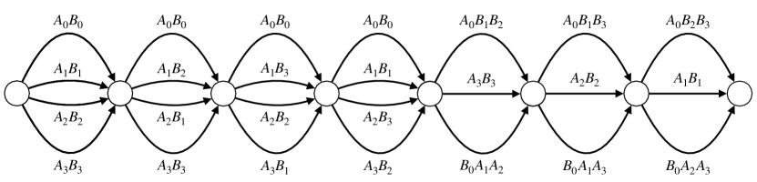
Figure 9: Paths $A_{i}$ and $B_{i}$ ($i\in\{0,1,2,3\}$), each edge being labeled with the paths it appears in. Assign to each path $A_{i}$ weight $a_{i}$, and to each path $B_{i}$ weight $b_{i}$, such that $a_{0}=b_{0}=3$, and $a_{i}=6^{2i}+1$ and $b_{i}=6^{2i+1}+5$ for $i=1,2,3$. Define the flow $X$ on $G$ as $X=\sum_{i=0}^{3}a_{i}A_{i}+\sum_{i=0}^{3}b_{i}B_{i}$. Note that these weights are a solution of $k$-FWA_N on input $(G,X)$ with given paths $A_{i}$, $B_{i}$ ($i\in\{0,1,2,3\}$).

We show that this conjecture is false using a counterexample. Consider the input for $k$-FWA_N from Figure 9 and the solution therein. We now give another solution for $k$-FWA_N on this input, namely the following path weights: $a_{0}=5,b_{0}=1$, and $a_{i}=6^{2i}+2,b_{i}=6^{2i+1}+4$, for $i=1,2,3$. One can easily verify that this is another solution to $k$-FWA_N on the input in Figure 9, thus proving that the rank of the corresponding linear system is strictly less than $8$.

To disprove 5.2, it remains to show that any flow decomposition contains at least $8$ paths. Due to the technicality of this proof (and its exhaustive case-by-case analysis), we only explain the intuition behind the construction in Figure 9 and behind the correctness proof. However, as an additional check we also ran both Toboggan [17] and a recently developed ILP solver for MFD_N [7] on this instance, both returning $\textsf{mfd}_{\mathbb{N}}(G,X)=8$.

The intuition is as follows. The graph can be divided into two parts: the graph induced by the first $5$ vertices in topological order (left part) and the one induced by the last $4$ (right part). We say that a path is fixed if every minimum flow decomposition of the graph contains this path. The paths $A_{i}$ and $B_{i}$ have expoentially growing weight for growing $i$ and get shuffled around with different permutations of the paired labels $A_{i}B_{j}$ on the left part. Due to the exponential growth, ensuring the correct parity on all edges of the right part, we can fix the paths $A_{i}$ and $B_{i}$ for $i=1,2,3$. This allows us to interpret flow decompositions of less than $8$ paths as decompositions with $8$ paths, where either $A_{0}$ or $B_{0}$ carries weight $0$. Consider a flow decomposition where we assign two paths of weights $\lambda_{1}$ and $\lambda_{2}$ on the edges labeled $A_{0}B_{0}$. For any $\delta\geq 0$, $(\lambda_{1}-\delta)+(\lambda_{2}+\delta)=a_{0}+b_{0}$ and equivalently for all other edges on the left part. If we decrease $\lambda_{1}$ by some $\delta>0$, the weights of $B_{1}$, $B_{2}$ and $B_{3}$ each increase by $\delta/2$. And thus, $\delta$ must be even. Due to the parity of $a_{0}$ and $b_{0}$, they can never reach $0$.

6 Conclusions

In this paper we have shown for the first time that width, a natural lower bound for MFD, is also useful when investigating its approximability. On the one hand, using width is a key insight in understanding where greedy path removal heuristics fail. On the other hand, graphs where width is well-behaved (e.g., series-parallel graphs) have a guaranteed approximation factor. Moreover, we generalised MFD to the problem to minimising the cost of a circluation decompisition, and showed that the integer version can be approximated even better by combining parity arguments of unitary circulations and a decomposition of such circulations of cost equal to the minimum cost to cover the graph. Finally, we have corroborated the complexity gap between the positive integer and the full integer case by disproving a conjecture from [17] (also motivating the heuristic in [23]), which would have had sped up their FPT algorithm for MFD_N.

Our results open up new avenues for further research on MFD. For example, can the width help find larger classes of graphs for which some greedy path removal (or even some sort of greedy path cover removal) algorithms have a guaranteed approximation factor? Can we get $\Omega(n)$ worst case approximation ratio of greedy-weight for dense graphs without parallel edges? Can the power-of-two decomposition approach be applied with other factors besides two? Can better path cover-like lower bounds help (e.g., path covers which cannot use an edge more times than its flow value, also computable in polynomial time)? How do our algorithms perform in practice?

7 Acknowledgements

This work was partially funded by the European Research Council (ERC) under the European Union’s Horizon 2020 research and innovation programme (grant agreement No. 851093, SAFEBIO), partially by the Academy of Finland (grants No. 322595, 328877, 352821, 346968), and partially by the National Science Foundation (NSF) (grants No. 1661530,1759522).

References

- [1] Ravindra K Ahujia, Thomas L Magnanti, and James B Orlin. Network flows: Theory, algorithms and applications. New Jersey: Prentice-Hall, 1993.
- [2] Jasmijn A Baaijens, Leen Stougie, and Alexander Schönhuth. Strain-aware assembly of genomes from mixed samples using flow variation graphs. In International Conference on Research in Computational Molecular Biology, pages 221–222. Springer, 2020.
- [3] Elsa Bernard, Laurent Jacob, Julien Mairal, and Jean-Philippe Vert. Efficient RNA isoform identification and quantification from RNA-Seq data with network flows. Bioinformatics, 30(17):2447–2455, 2014.
- [4] Dimitris Bertsimas, Ebrahim Nasrabadi, and Sebastian Stiller. Robust and adaptive network flows. Operations Research, 61(5):1218–1242, 2013. arXiv:https://doi.org/10.1287/opre.2013.1200, doi:10.1287/opre.2013.1200.
- [5] Manuel Cáceres, Massimo Cairo, Brendan Mumey, Romeo Rizzi, and Alexandru I. Tomescu. Sparsifying, shrinking and splicing for minimum path cover in parameterized linear time. In SODA 2022 - ACM-SIAM Symposium on Discrete Algorithms, pages 359–376, 2022. URL: https://epubs.siam.org/doi/abs/10.1137/1.9781611977073.18, doi:10.1137/1.9781611977073.18.
- [6] Fernando HC Dias, Manuel Caceres, Lucia Williams, Brendan Mumey, and Alexandru I Tomescu. A safety framework for flow decomposition problems via integer linear programming. arXiv preprint arXiv:2301.13245, 2023.
- [7] Fernando HC Dias, Lucia Williams, Brendan Mumey, and Alexandru I Tomescu. Fast, flexible, and exact minimum flow decompositions via ilp. In Research in Computational Molecular Biology: 26th Annual International Conference, RECOMB 2022, San Diego, CA, USA, May 22–25, 2022, Proceedings, pages 230–245. Springer, 2022.
- [8] Robert P Dilworth. A decomposition theorem for partially ordered sets. Annals of Mathematics, 51(1):161–166, 1950. URL: http://www.jstor.org/stable/1969503.
- [9] David Eppstein. Parallel recognition of series-parallel graphs. Information and Computation, 98(1):41–55, 1992. URL: https://www.sciencedirect.com/science/article/pii/089054019290041D, doi:10.1016/0890-5401(92)90041-D.
- [10] Delbert R Fulkerson. Note on Dilworth’s decomposition theorem for partially ordered sets. Proceedings of the American Mathematical Society, 7(4):701–702, 1956.
- [11] Harold N Gabow and Robert E Tarjan. Faster scaling algorithms for network problems. SIAM Journal on Computing, 18(5):1013–1036, 1989.
- [12] Marcelo Garlet Millani, Hendrik Molter, Rolf Niedermeier, and Manuel Sorge. Efficient algorithms for measuring the funnel-likeness of dags. Journal of Combinatorial Optimization, 39:216–245, 2020.
- [13] Thomas Gatter and Peter F Stadler. Ryūtō: network-flow based transcriptome reconstruction. BMC bioinformatics, 20(1):1–14, 2019.
- [14] Tzvika Hartman, Avinatan Hassidim, Haim Kaplan, Danny Raz, and Michal Segalov. How to split a flow? In 2012 Proceedings IEEE INFOCOM, pages 828–836. IEEE, 2012.
- [15] A. Jain and N. Chandrasekharan. An efficient parallel algorithm for min-cost flow on directed series-parallel networks. In Proceedings Seventh International Parallel Processing Symposium, pages 188–192, 1993. doi:10.1109/IPPS.1993.262879.
- [16] Shahbaz Khan, Milla Kortelainen, Manuel Cáceres, Lucia Williams, and Alexandru I Tomescu. Improving rna assembly via safety and completeness in flow decompositions. Journal of Computational Biology, 29(12):1270–1287, 2022.
- [17] Kyle Kloster, Philipp Kuinke, Michael P O’Brien, Felix Reidl, Fernando Sánchez Villaamil, Blair D Sullivan, and Andrew van der Poel. A practical fpt algorithm for flow decomposition and transcript assembly. In 2018 Proceedings of the Twentieth Workshop on Algorithm Engineering and Experiments (ALENEX), pages 75–86. SIAM, 2018.
- [18] Brendan Mumey, Samareh Shahmohammadi, Kathryn McManus, and Sean Yaw. Parity balancing path flow decomposition and routing. In 2015 IEEE Globecom Workshops (GC Wkshps), pages 1–6. IEEE, 2015.
- [19] Nils Olsen, Natalia Kliewer, and Lena Wolbeck. A study on flow decomposition methods for scheduling of electric buses in public transport based on aggregated time–space network models. Central European Journal of Operations Research, 2020. doi:10.1007/s10100-020-00705-6.
- [20] James B. Orlin. Max flows in O(nm) time, or better. In Dan Boneh, Tim Roughgarden, and Joan Feigenbaum, editors, Symposium on Theory of Computing Conference, STOC’13, Palo Alto, CA, USA, June 1-4, 2013, pages 765–774. ACM, 2013. doi:10.1145/2488608.2488705.
- [21] Mihaela Pertea, Geo M Pertea, Corina M Antonescu, Tsung-Cheng Chang, Joshua T Mendell, and Steven L Salzberg. StringTie enables improved reconstruction of a transcriptome from RNA-seq reads. Nature biotechnology, 33(3):290–295, 2015.
- [22] Alexander Schrijver. Theory of Linear and Integer Programming. John Wiley & Sons, Inc., 1986.
- [23] Mingfu Shao and Carl Kingsford. Theory and a heuristic for the minimum path flow decomposition problem. IEEE/ACM transactions on computational biology and bioinformatics, 16(2):658–670, 2017.
- [24] Mingxiang Teng, Michael I Love, Carrie A Davis, Sarah Djebali, Alexander Dobin, Brenton R Graveley, Sheng Li, Christopher E Mason, Sara Olson, Dmitri Pervouchine, et al. A benchmark for rna-seq quantification pipelines. Genome biology, 17(1):1–12, 2016.
- [25] Alexandru I Tomescu, Travis Gagie, Alexandru Popa, Romeo Rizzi, Anna Kuosmanen, and Veli Mäkinen. Explaining a weighted DAG with few paths for solving genome-guided multi-assembly. IEEE/ACM transactions on computational biology and bioinformatics, 12(6):1345–1354, 2015.
- [26] Alexandru I Tomescu, Anna Kuosmanen, Romeo Rizzi, and Veli Mäkinen. A novel min-cost flow method for estimating transcript expression with RNA-Seq. In BMC bioinformatics, volume 14, pages S15:1–S15:10. Springer, 2013.
- [27] Jacobo Valdes, Robert E. Tarjan, and Eugene L. Lawler. The recognition of series parallel digraphs. SIAM Journal on Computing, 11(2):298–313, 1982. arXiv:https://doi.org/10.1137/0211023, doi:10.1137/0211023.
- [28] Benedicte Vatinlen, Fabrice Chauvet, Philippe Chrétienne, and Philippe Mahey. Simple bounds and greedy algorithms for decomposing a flow into a minimal set of paths. European Journal of Operational Research, 185(3):1390–1401, 2008.
- [29] Lucia Williams, Gillian Reynolds, and Brendan Mumey. RNA Transcript Assembly Using Inexact Flows. In 2019 IEEE International Conference on Bioinformatics and Biomedicine (BIBM), pages 1907–1914. IEEE, 2019.