EasyABM: a lightweight and easy to use heterogeneous agent-based modelling tool written in Julia.

Abstract

Agent based modelling is a computational approach that aims to understand the behaviour of complex systems through simplified interactions of programmable objects in computer memory called agents. Agent based models (ABMs) are predominantly used in fields of biology, ecology, social sciences and economics where the systems of interest often consist of several interacting entities. In this work, we present a Julia package EasyABM.jl for simplifying the process of studying agent based models. EasyABM.jl provides an intuitive and easy to understand functional approach for building and analysing agent based models.

1 Introduction

Agent based modelling is a computataional paradigm in which autonomous interacting entities called agents are evolved in time according to predefined rules with an aim to understand emergent phenomena in complex systems. Agent based modelling has a diverse range of applications in economics, social behaviour, biology, epidemiology and ecology. In particular, agent based models (ABMs) have been used to study pandemics Nic2020 ; Hinch2021 ; Kerr2021 , population dynamics SM2014 ; Jang2016 , biofilms Lardon2011 , tumor growth Jan2016 , financial markets Sam2020 ; Feng2012 as well as societal phenomena such as urbanisation Mau2021 , traffic flows Hager2015 and migration Anna2016 ; Jule2018 .

Depending on the application, an agent in an ABM can represent an organism, institution, a physical object or an abstract entity. There is generally no central control system in ABMs and agents act independently according to the rules of the model. Surprisingly, even simple rules of dynamics can lead to interesting emergent phenomena which is a key driving principle behing the usefulness of ABMs in understanding complex systems.

Several frameworks and tools have been developed for agent based modelling. Some of the general purpose ABM frameworks include NetLogo Wilensky1999 , Mesa DMas2015 , Agents George2022 , MASON SLuk2005 , Swarm HIba2013 and Repast MJ2013 . All these frameworks use different programming languages and follow different design principles. Until now, Agents.jl has been the only ABM framework written in Julia. Our objective in developing EasyABM.jl has been to provide Julia users interested in agents based modelling with an alternate tool. EasyABM.jl follows a completely different design principle from Agents.jl. The API of EasyABM takes a function based approach where for each modelling task from creating agents and model, to running model and creating visualisation, there is a function to accomplish the task. Agents.jl is similar except that one needs to use a struct for creating agents. Even though it leads to a more performant code, the idea of a struct may not be easily comprehensible for people with only a basic background in programming. Another aspect of Agents.jl which, in our opinion, makes it somewhat complex to understand for new users is two different types of step functions (agent_step! and model_step!) that can be used for simulation, compared to only one step function (step_rule!) in EasyABM. Visualisation is another area where EasyABM takes relatively more intuitive approach compared to Agents.jl. In EasyABM the graphics properties are associated with agents at the time of definition of agents or at model initialisation step and later can be manipulated during model run. Visualisation can then by done by a single function call whereas in Agents.jl it takes more effort.

The figure 1 gives a diagrammatic representation of agents based modelling workflow with EasyABM. In the next section we explain this workflow with some examples of agents based models.

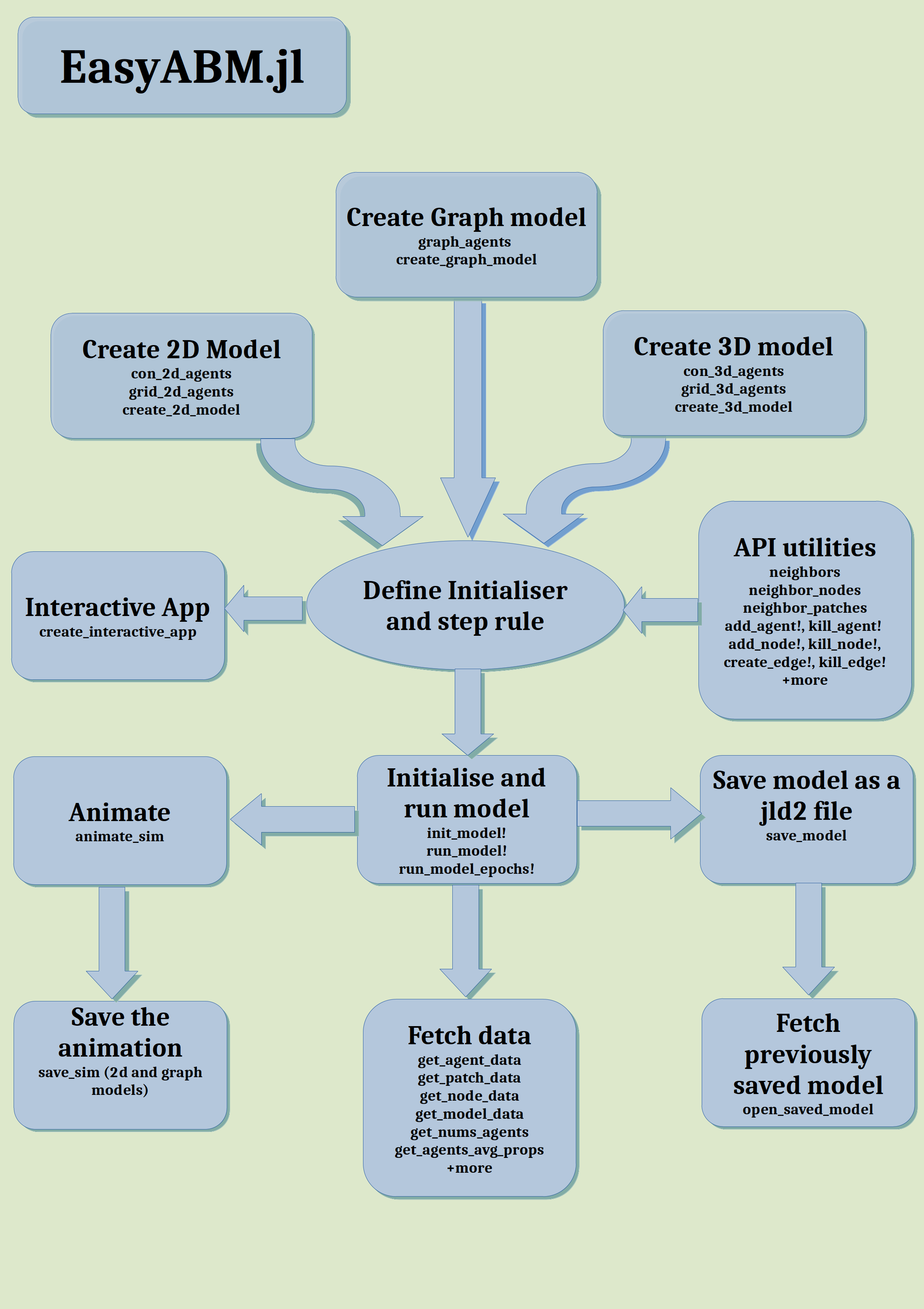
Figure 1: Agents based modelling workflow with EasyABM.

2 Agent based modelling with EasyABM

EasyABM.jl allows users to create and study models in 2D, 3D and graph spaces. In the 2D and 3D models there can be two types of agents - grid agents which can move only in discrete steps and continuous agents which can move continuously. Moreover, both in 2D and 3D models the space is divided into unit blocks called patches where each patch can have its own properties like agents. This feature of EasyABM.jl has been inspired by NetlogoWilensky1999 . Nodes and edges in a graph space can also be assigned properties similar to agents. A graph space can be chosen to be fully dynamic in which nodes and edges can be added or removed during time evolution.

In the present section we explain the workflow of EasyABM, as outlined in Figure 1, through flocking model in 2D, Schelling’s segregation model in 3D and Ising model on a nearest neighbor graph for graph spaces. For more details on these and many other models in EasyABM we refer to the examples in the online documentation.

2.1 2D models

EasyABM uses functional approach for creation of agents and models. The code in listing 1 uses the function con_2d_agents to create 200 continuous space 2D agents with properties shape, pos, vel and orientation and then creates the model using create_2d_model function. For a grid based 2D model one needs grid agents which can be created using grid_2d_agents function.

Listing 1: Flocking in 2D - Defining agents and the model.

⬇

using EasyABM

boids = con_2d_agents(200,

shape = :arrow, pos = Vect(0.0,0.0),

vel=Vect(0.0,0.0), orientation = 0.0,

keeps_record_of = [:pos, :vel,

:orientation])

model = create_2d_model(boids,

agents_type=Static,

space_type = Periodic,

min_dis = 0.3, coh_fac = 0.05,

sep_fac = 0.5, dt= 0.1,

vis_range = 2.0, aln_fac = 0.35)

EasyABM recognises pos as position and vel as velocity of the agent. The property pos must be a Vect which is an inbuilt vector type of EasyABM. It is also convenient to use Vect for any other vectorial properties in the model like velocity or forces. The properties shape and orientation are also recognised by EasyABM as graphics properties of agents. The keeps_record_of argument is the list of properties that the agent will record during time evolution. The agents in EasyABM are fully hetrogeneous in that each agent can have different set of properties of which it can record any specified subset during model run. The list of agents, that we have named as boids for the flocking model, is supplied as the first argument in the function create_2d_model for creating model. The argument agents_type is set to Static if the number of agents remain fixed during simulation and Mortal if the agents can take birth or die. The space_type property is set to Periodic if the space is periodic in all directions and NPeriodic for a non-periodic space. Other arguments of the create_2d_model function are parameters specific to the flocking simulation:

• min_dis : The distance between boids below which they start repelling each other.

• coh_fac : The proportionality constant for the cohere force.

• sep_fac : The proportionality constant for the separation force.

• aln_fac : The proportionality constant for the alignment force.

• vis_range : The visual range of boids.

• dt : The proportionality constant between change in position and velocity.

After creating the model, the initial properties of agents can be set through an initialiser function which is then sent as an argument to init_model! function provided by EasyABM.jl. The code for the initialiser function for 2D flocking model in shown in listing 2

Listing 2: Flocking in 2D - Initialiser function.

⬇

function initialiser!(model)

xdim, ydim = model.size

for boid in model.agents

boid.pos = Vect(rand()*xdim, rand()*ydim)

boid.orientation = rand()*2*3.14

boid.vel = Vect(-sin(boid.orientation),

cos(boid.orientation))

end

end

init_model!(model, initialiser = initialiser!)

The next step is to define rules of dynamics through a step_rule! function and run the model. The step_rule! function for the flocking model is shown in listing 3.

Listing 3: Defining step rule and running the model.

⬇

const ep = 0.00001

function step_rule!(model)

dt = model.parameters.dt

min_dis = model.parameters.min_dis

aln_fac = model.parameters.aln_fac

coh_fac = model.parameters.coh_fac

sep_fac = model.parameters.sep_fac

for boid in model.agents

nbrs = euclidean_neighbors(boid, model,

model.parameters.vis_range)

coh_force = Vect(0.0,0.0)

sep_force = Vect(0.0,0.0)

aln_force = Vect(0.0,0.0)

num = 0

for nbr in nbrs

num+=1

vec = nbr.pos - boid.pos

if veclength(vec)< min_dis

sep_force -= vec

end

coh_force += vec

aln_force += nbr.vel

end

if num>0

aln_force = (aln_force/ num -

boid.vel)*aln_fac

coh_force *= coh_fac/num

sep_force *= sep_fac

boid.vel += (coh_force + sep_force) + aln_force

boid.vel /= (veclength(boid.vel)+ep)

boid.orientation = calculate_direction(boid.vel)

end

boid.pos += boid.vel*dt

end

end

run_model!(model, steps=500,

step_rule = step_rule!)

With the data collected during model run, the animation can be created with a single line of code as shown below. The output of this line of code is an interactive animation as shown in Figure 2. The save button can be used to save the animation to the path mentioned in the animate_sim function.

⬇

animate_sim(model, path = "/path/to/folder/anim.gif")

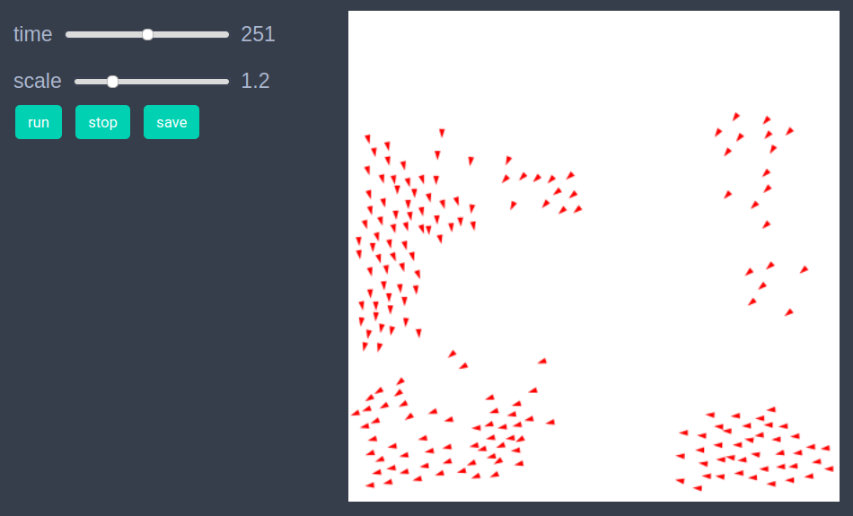
Figure 2: Visualisation for flocking model. The size of agents can be changed with the size slider. Save button can be used for saving the animation.

EasyABM also makes it very easy to create an interactive application for the model in Jupyter and similar notebook environments with WebIO installation. The following lines of code create an interactive app for the flocking model as shown in Figure 3.

⬇

create_interactive_app(model,

initialiser= initialiser!,

step_rule= step_rule!,

model_controls=

[(:min_dis, :s, 0.01:0.1:1.0),

(:coh_fac, :s, 0.01:0.01:1.0),

(:sep_fac, :s, 0.01:0.01:1.0),

(:aln_fac, :s, 0.01:0.01:1.0),

(:vis_range, :s, 0.5:0.5:4.0)],

agent_plots=Dict("boids to the left"=>

boid -> boid.pos[1]<model.size[1]/2),

frames=400)

Finally, EasyABM.jl API provides functions to fetch data of individual agents and also data averaged over all agents. For example the data of the agent with index 1, can be fetched as

⬇

df = get_agent_data(model.agents[1], model).record

Similarly, the average velocity of agents at all times during model run can be obtained as

⬇

df = get_agents_avg_props(model,

agent -> agent.vel,

labels = ["average velocity"])

Similar functions are also available for fetching data of patches, nodes and edges.

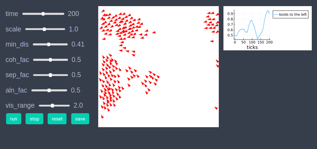
Figure 3: Interactive app for flocking model. Sliders can be used to change model parameters and then the model can be reset and run again. The plot on the right shows fraction of boids which are in the left half of the space.

2.2 3D models

Just as for 2D models, in 3D too EasyABM.jl provides simple functions to accomplish modelling tasks. We explain its use in 3D through the 3D version of Schelling’s segregation model. In the Schelling’s model agents live on a grid. The code below uses the function grid_3d_agents to create 200 3D-grid agents with properties color, pos and mood and then uses function create_3d_model to create the model. For a model requiring a continuous 3D space agents can be created using con_3d_agents function, while the function for creating model remains the same.

⬇

using EasyABM

@enum agentsfeeling happy sad

agents = grid_3d_agents(200, pos = Vect(1,1,1),

color = :red, mood = happy,

keeps_record_of=[:pos, :mood])

model = create_3d_model(agents,

agents_type = Static,

space_type = NPeriodic,

size = (7,7,7), min_alike = 8)

For grid type agents the position vector is required to have integer valued coordinates. The mood of agents is an enum property which can take only two values - happy or sad. Also through keeps_record_of argument, we are asking agents to record their position and mood properties during time evolution. Similar to create_2d_model function, the function create_3d_model also accepts the list of agents as the first argument. Since the number of Schelling’s agents remain fixed during simulation we set the argument agents_type to Static. We also set space_type property to NPeriodic for a non-periodic 3D space. The argument min_alike is a model property specific to the Schelling’s model and we set its value to 8.

After creating the model, the initial properties of agents can be set through an initialiser function which is then sent as an argument to init_model! function provided by EasyABM.jl. The code for the initialiser function for 2D flocking model in shown below.

⬇

function initialiser!(model)

for agent in model.agents

agent.color = [:red, :green][rand(1:2)]

x,y,z = random_empty_patch(model)

agent.pos = Vect(x, y, z)

end

for agent in model.agents

nbrs = grid_neighbors(agent, model, 1)

num_same = 0

for nbr in nbrs

if nbr.color == agent.color

num_same += 1

end

end

if num_same < model.parameters.min_alike

agent.mood = sad

end

end

end

init_model!(model, initialiser = initialiser!)

The step_rule! function for the 3D Schelling’s model is shown in listing 4. This function is then passed as an argument to the run_model! function to run it for required number of steps.

Listing 4: Schelling’s segregation in 3D - step rule.

⬇

function step_rule!(model)

min_alike = model.parameters.min_alike

for agent in model.agents

num_alike = 0

for nbr in neighbors(agent, model,1)

if agent.color == nbr.color

num_alike += 1

end

end

if num_alike >= min_alike

agent.mood = happy

else

agent.mood = sad

x,y,z = random_empty_patch(model)

agent.pos = Vect(x, y, z)

end

end

return

end

run_model!(model, steps=200,

step_rule = step_rule!)

EasyABM.jl uses MeshCat.jl as backend for 3D visualisations. Animation from the data collected during model run can be created with the animate_sim function as in case of 2D models.

Creating an interactive application also requires a single function call with intuitive and easy to understand arguments. The following function creates an interactive app for the Schelling’s 3D model as shown in Figure 5.

⬇

create_interactive_app(model,

initialiser= initialiser!,

step_rule=step_rule!,

model_controls=[(:min_alike, :s, 1:12)],

agent_plots=Dict(

"happy"=> agent-> agent.mood == happy,

"sad"=> agent-> agent.mood == sad

),

frames=200)

Data of individual agents, as well as average properties of agents can be fetched via simple function calls. The code below fetches the data of number of happy and sad agents at each time step as a dataframe and plots the result as shown in Fig 4.

⬇

df = get_nums_agents(model,

agent-> agent.mood == happy,

agent-> agent.mood == sad,

labels=["happy","sad"],

plot_result=true)

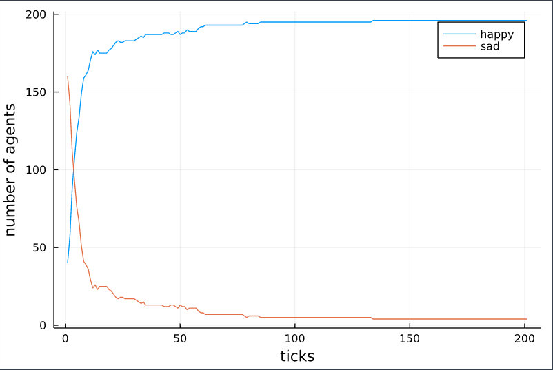
Figure 4: Plot of number of happy and sad agents along time evolution of Schelling’s 3D model.

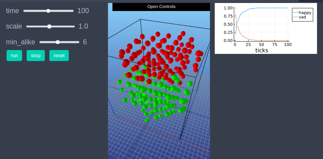
Figure 5: Interactive app for Schelling’s 3D model. The plot on the right shows fraction of happy and sad agents in the model as the time progresses.

2.3 Graph based models

Graph spaces in EasyABM.jl can be either static or dynamic. The topology of a static graph remains fixed during model run, while that of a dynamic graph can be changed. Graphs created with other julia packages like Graphs.jl can be used in graph based models after converting them to static or dynamic type using inbuilt EasyABM functionality. In this subsection we explain the workflow for graph based models using example of Ising model on nearest neighbor graphs. In graph based models agents can be created using graph_agents function and then included in the model in the same way as in the case of 2D and 3D models. However, for the Ising model, we will not need any agents and would rather attach spin property to the nodes of the graph. As shown in the code below, we define the model by creating an empty graph and using create_graph_model function with the graph as the first argument. We set the agents_type to Static as the number of agents is fixed to be zero. There are three parameters temp, coupl and nns in the model where temp and coupl are respectively the temperature and coupling parameters of the Ising model and nns is the number of nearest nodes that each node will have an edge with in the graph.

⬇

graph = dynamic_simple_graph(0)

model = create_graph_model(graph,

agents_type = Static,

temp = 2.0, coupl = 2.5,

nns = 5)

In the code for initialisation, as shown in listing 5, we use NearestNeighbors.jl package and define an initiliser function where a nearest neighbor graph of a fixed number of nodes is created and its nodes are randomly assigned with spin and color properties, where we assign black color to nodes with spin 1, and white color to nodes with spin -1. The properties spin and color of nodes that we want to be recorded during model run are specified in the props_to_record argument in the init_model! function.

Listing 5: Ising model on nearest neighbor graph - initialisation.

⬇

using NearestNeighbors

const n = 500;

function initialiser!(model)

vecs = rand(2, n)

kdtree = KDTree(vecs,leafsize=4)

flush_graph!(model)

add_nodes!(n, model, color = :black, spin =1)

for i in 1:n

model.graph.nodesprops[i].pos = (vecs[1,i], vecs[2,i])

indices, _ = knn(kdtree,

vecs[:,i],

model.parameters.nns, true)

for j in indices

if j!=i

create_edge!(i,j, model)

end

end

if rand()<0.5

model.graph.nodesprops[i].spin = 1

model.graph.nodesprops[i].color = :black

else

model.graph.nodesprops[i].spin = -1

model.graph.nodesprops[i].color = :white

end

end

end

init_model!(model, initialiser= initialise!,

props_to_record = Dict("nodes"=>[:color, :spin]))

In the step rule of the Ising model as shown in listing 6, we carry out a fixed number of Monte-Carlo steps in which a node is selected at random and its spin and color are flipped depending on the usual Ising energy condition. Then we run the model for 100 steps using the run_model! function and sending step_rule! as an argument.

Listing 6: Ising model on nearest neighbor graph - step run.

⬇

function step_rule!(model)

nodesprops = model.graph.nodesprops

for i in 1:100

rand_nd = rand(1:n)

spin = nodesprops[random_node].spin

nbr_nodes = neighbor_nodes(rand_nd, model)

de = 0.0

for node in nbr_nodes

nbr_spin = nodesprops[node].spin

de += spin*nbr_spin

end

de = 2*model.parameters.coupl * de

if (de < 0) || (rand() < exp(-de/model.parameters.temp))

nodesprops[random_node].spin = - spin

nodesprops[random_node].color = spin == -1 ? :black : :white

end

end

end

run_model!(model, steps = 100, step_rule = step_rule!)

Tasks of creating an animation and interactive app for graph models uses the same functions as in 2D and 3D case. For example, the code below will create an interactive app for the Ising model as shown in Fig 6

⬇

create_interactive_app(model,

initialiser= initialiser!,

props_to_record =

Dict("nodes"=>[:color, :spin]),

step_rule= step_rule!,

model_controls=[

(:temp, :s, 0.05:0.05:5.0),

(:coupl, :s, 0.01:0.1:5.0),

(:nns, :s, 2:10)],

node_plots = Dict("magnetisation"=>

x -> x.spin),

frames=100)

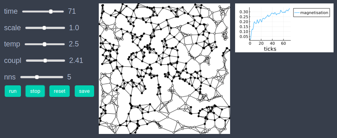
Figure 6: Interactive app for Ising model on a nearest neighbor graph. Sliders can be used to change the model paramters and then the model can be re-initialised with the reset button.

EasyABM.jl API provides simple functions for fetching data of individual agents, nodes and edges as in case of 2D and 3D models. For example, the code below fetches the data of average spin of nodes (also called magnetisation) as a dataframe and plots the result as shown in Fig 7.

⬇

df = get_nodes_avg_props(model,

node -> node.spin,

labels=["magnetisation"],

plot_result = true)

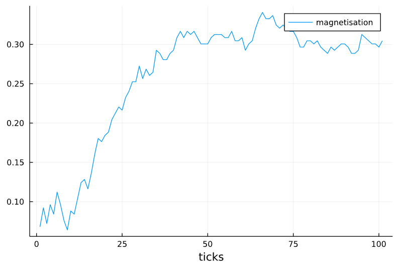
Figure 7: Plot of magnetisation vs time for the Ising model.

3 Conclusions and future work

We have introduced a new Julia framework for agents based modelling and explained its workflow with examples of 2D, 3D and graph based models. Some of the notable features of EasyABM we have tried to emphasise are -

• Fully function based approach.

• Intuitive visualisation.

• Easy data collection.

• Patches of space, and nodes and edges of graph can be assigned properties like agents.

• Dynamic graph spaces.

Some of the future plans for EasyABM are -

• Inclusion of more inbuilt graph types (current version only has some inbuilt grid graphs).

• Providing more than one backend options for visualisations in 2D, 3D and graph models.

• Visualisation of graphs in 3D space.

• Expanding documentation by including more examples.

Users of EasyABM are also welcome to contribute to the package by suggesting or adding new features, improving documentation and reporting bugs.

References

- (1) Nicolas Hoertel, Martin Blachier, Carlos Blanco, Mark Olfson, Marc Massetti, Marina Sánchez Rico, Frédéric Limosin and Henri Leleu, A stochastic agent-based model of the SARS-CoV-2 epidemic in France, Nature Medicine, vol. 26, pp. 1417–1421, 2020.
- (2) Hinch R, Probert WJM, Nurtay A, Kendall M, Wymant C, Hall M, et al., OpenABM-Covid19-An agent-based model for non-pharmaceutical interventions against COVID-19 including contact tracing, PLoS Computational Biology, vol. 17, issue 7, 2021.
- (3) Kerr CC, Stuart RM, Mistry D, Abeysuriya RG, Rosenfeld K, Hart GR, et al., Covasim: An agent-based model of COVID-19 dynamics and interventions, PLoS Computational Biology, vol. 17, issue 7, 2021.
- (4) SM Niaz Arifin, Ying Zhou, Gregory J. Davis, James E. Gentile, Gregory R. Madey and Frank H. Collins, An agent-based model of the population dynamics of Anopheles gambiae, Malaria Journal, vol. 13, Article number 424, 2014.
- (5) Jang Won Bae, Euihyun Paik. Kiho Kim, Karandeep Singh and Mazhar Sajjad, Combining Microsimulation and Agent-based Model for Micro-level Population Dynamics, Procedia Computer Science, vol. 80, pp. 507–517, 2016.
- (6) Lardon LA, Merkey BV, Martins S, Dötsch A, Picioreanu C, Kreft JU, Smets BF, iDynoMiCS: next-generation individual-based modelling of biofilms, Environmental Microbiology. vol. 13, issue 9, pp. 2416–2434, September 2011.
- (7) Jan Poleszczuk, Paul Macklin and Heiko Enderling, Agent-Based Modeling of Cancer Stem Cell Driven Solid Tumor Growth, Methods in Molecular Biology, vol. 1516, pp. 335–346, 2016.
- (8) Samuel Vanfossan, Cihan H. Dagli and Benjamin Kwasa, An Agent-Based Approach to Artificial Stock Market Modeling, Procedia Computer Science, vol. 168, pp. 161–169, 2020.
- (9) Ling Feng, Baowen Li, Boris Podobnik, Tobias Preis, and H. Eugene Stanley, Linking agent-based models and stochastic models of financial markets, Applied Physical Science, PNAS, vol. 109, issue 22, May 2012.
- (10) Karsten Hager, Jürgen Rauh and Wolfgang Rid, Agent-based Modeling of Traffic Behavior in Growing Metropolitan Areas, Transportation Research Procedia, vol. 10, pp. 306–315, 2015.
- (11) Mauricio González-Méndez, Camilo Olaya, Isidoro Fasolino, Michele Grimaldi and Nelson Obregón, Agent-Based Modeling for Urban Development Planning based on Human Needs. Conceptual Basis and Model Formulation, Land Use Policy, vol. 101, Feb 2021.
- (12) Anna Klabunde and Frans Willekens, Decision-Making in Agent-Based Models of Migration: State of the Art and Challenges, European Journal of Population, vol. 32, pp. 73–97, Feb 2016.
- (13) Jule Thober, Nina Schwarz and Kathleen Hermans, Agent-based modeling of environment-migration linkages: a review, Ecology and Society, vol. 23, issue 2, June 2018.
- (14) L. Wilensky, Netlogo, Center for Connected Learning and Computer-Based Modeling, Northwestern University, 1999.
- (15) S. Luke, C. Cioffi-Revilla, L. Panait, K. Sullivan, and G. Balan, MASON: A Multiagent Simulation Environment, SIMULATION, vol. 81, pp. 517–527, July 2005.
- (16) M. J. North, N. T. Collier, J. Ozik, E. R. Tatara, C. M. Macal, M. Bragen, and P. Sydelko, Complex adaptive systems modeling with Repast Simphony, Complex Adaptive Systems Modeling, vol. 1, p. 3, Dec. 2013.
- (17) H. Iba, Agent-Based Modeling and Simulation with Swarm, Chapman and Hall/CRC, zeroth ed., June 2013.
- (18) D. Masad and J. Kazil, Mesa: An Agent-Based Modeling Framework, Python in Science Conference, pp. 51–58, 2015.
- (19) George Datseris and Ali R. Vahdati and Timothy C. DuBois Agents.jl: a performant and feature-full agent-based modeling software of minimal code complexity, Simulation, Sage Journals, 2022.
- (20) Renu Solanki, Monisha Khanna Kapur, Shailly Anand, Anita Gulati, Prateek Kumar, Munendra Kumar and Dushyant Kumar, EasyABM.jl github repository documentation. .