Second-order corrections to Starobinsky inflation

Abstract

Higher-order theories of gravity are extensions to general relativity (GR) motivated mainly by high-energy physics searching for GR ultraviolet completeness. They are characterized by the inclusion of correction terms in the Einstein-Hilbert action that leads to higher-order field equations. In this paper, we propose investigating inflation due to the GR extension built with all correction terms up to the second-order involving only the scalar curvature $R$, namely, $R^{2}$, $R^{3}$, $R\square R$. We investigate inflation within the Friedmann cosmological background, where we study the phase space of the model, as well as explore inflation in slow-roll leading-order. Furthermore, we describe the evolution of scalar perturbations and properly establish the curvature perturbation. Finally, we confront the proposed model with recent observations from Planck, BICEP3/Keck, and BAO data.

I Introduction

Despite the immense predictive power of general relativity (GR), extensions to it have been motivated by several areas. In high-energy physics, which aims for the ultraviolet completeness of GR, quantum gravity and inflation models are included. On the other hand, models involving low-energy physics include, among others, the phenomenology of the dark sector of the universe and spherically symmetric solutions in a weak-field regime.

According to Lovelock’s theorem, fundamentally, GR is constructed based on some hypotheses: it is a $4$-dimensional Riemannian metric gravity theory, containing the metric $g_{\mu\nu}$ as the only fundamental field, invariant by diffeomorphism and with second-order field equations. In this sense, extensions to GR are achieved by violating any of these hypotheses [1]. By violating the first hypothesis, we can allow a higher-dimensional spacetime or even consider a gravitational action constructed with curvature and torsion invariants due to a Riemann-Cartan spacetime [2]. If we violate the hypothesis that the theory of gravity has the metric as the only fundamental field, we can obtain, for example, the Horndeski theories. These, in turn, are the more general $4$-dimensional theories of gravity whose action, constructed with the metric and a scalar field, leads to second-order field equations [3]. On the other hand, by allowing field equations above the second-order and preserving all other assumptions, we find the higher-order gravities.

Higher-order theories of gravity are characterized by the inclusion of correction terms in the Einstein-Hilbert (EH) action that lead to higher-order field equations. Such corrections can be conveniently classified according to their mass (energy) scale. In this scenario, EH plus the cosmological constant represents the usual zero-order term. First-order corrections to EH are fourth mass terms constructed from the $4$ possible invariants

$$R^{2}\text{, }R_{\mu\nu}R^{\mu\nu}\text{, }R_{\mu\nu\alpha\beta}R^{\mu\nu\alpha\beta}\text{ \ and }\square R.$$

In turn, the second-order corrections to EH are sixth mass terms, built with the invariants

$$R\square R\text{, }R_{\mu\nu}\square R^{\mu\nu}\text{,}$$

$$R^{3}\text{, }RR_{\mu\nu}R^{\mu\nu}\text{, }R_{\mu\nu}R_{\text{ \ }\alpha}^{\nu}R^{\alpha\mu}\text{,}$$

$$RR_{\mu\nu\alpha\beta}R^{\mu\nu\alpha\beta}\text{, }R_{\mu\alpha}R_{\nu\beta}R^{\mu\nu\alpha\beta}\text{ \ and }R_{\mu\nu\alpha\beta}R_{\text{ \ \ }\kappa\rho}^{\alpha\beta}R^{\kappa\rho\mu\nu}.$$

And so on, we will have more higher-order correction terms as we increase the energy scales.

Models involving higher-order gravities have been explored in various contexts. There are papers in the literature whose purpose is to show the equivalence between different classes of gravity theories, in particular, between $f\left(R\right)$ or $f\left(R,\square^{k}R\right)$ and scalar-tensor theories [4, 5, 6, 7, 8, 9, 10]. In some contexts, it becomes more convenient to pass from the original frame to the Jordan or Einstein frames, through a conformal transformation, in order to handle equations for scalar fields rather than higher-order equations for the metric. Another topic of great interest is the investigation of spherically symmetric and static solutions in higher-order gravities, with Stelle’s paper [11] being one of those responsible for shedding light on this line of research. In particular, the study of the possibility of non-Schwarzschild black hole solutions through different approaches is addressed in Refs. [12, 13, 14, 15, 16, 17, 18, 19], whereas researches involving weak-field regime solutions are covered in Refs. [20, 21, 22, 19]. There are also models that study the generation and properties of gravitational waves [23, 24, 25, 26, 27, 28, 29, 30, 31, 32, 33]. The latter is a topic of great current appeal due to the direct detections [34, 35, 36] that allow the rising of gravitational wave astrophysics.

Regarding inflation, it is well known in the literature that the Starobinsky model [37, 38] has a good fit for recent observational data from Planck, BICEP3/Keck and BAO [39, 40]. Furthermore, the fact that it has a well-grounded theoretical motivation makes it one of the strongest inflationary candidates, despite the immense plethora of inflation models [41]. Such reasons motivate the investigation of models based on extensions to the Starobinsky model via higher-order gravity theories. There is a large amount of research in this context. Some of them are based on $f\left(R\right)$ theories, as in Refs. [42, 43, 44, 45, 46, 47], others consider the introduction of Weyl’s term [48, 49, 50, 51, 52]. There are those that consider local gravitational actions involving a finite number of curvature derivative terms [53, 54, 55, 56, 57, 58, 59], while others are nonlocal, involving infinite derivatives [60, 61, 62, 63, 64].

In this paper, we propose to investigate the extension to the Starobinsky model due to the inclusion of all correction terms up to the second-order involving only the scalar curvature $R$. In this sense, we have the following gravitational action

$$S=\frac{M_{Pl}^{2}}{2}\int d^{4}x\sqrt{-g}\left(R+\frac{1}{2\kappa_{0}}R^{2}+\frac{\alpha_{0}}{3\kappa_{0}^{2}}R^{3}-\frac{\beta_{0}}{2\kappa_{0}^{2}}R\square R\right),$$ (1)

where $\kappa_{0}$ has squared mass unit and parameters $\alpha_{0}$ and $\beta_{0}$ are dimensionless quantities. Furthermore, $M_{Pl}$ is the reduced Planck mass, such that $M_{Pl}^{2}\equiv\left(8\pi G\right)^{-1}$ and $\square\equiv\nabla_{\sigma}\nabla^{\sigma}$ represents the covariant d’Alembertian operator. In this scenario, where we only address the scalar sector of corrections, $R^{2}$ represents the first-order correction, while the last two terms correspond to the second-order corrections to EH. Note that the parameter $\kappa_{0}$ is responsible for establishing the energy scale of inflation, while the parameters $\alpha_{0}$ and $\beta_{0}$ give us a measure of the Starobinsky deviation. Since $R^{3}$ and $R\square R$ are both second-order correction terms on energy scales, they must contribute similarly to inflation, so there is a joint effect that must be considered. In that regard, it is worth noting that our paper goes a step further in recent researches developed in [44] and [58, 59], which address the models Starobinsky$+R^{3}$ and Starobinsky$+R\square R$, respectively. In this paper, the multi-field treatment associated with the $R\square R$ term is different from that used in Ref. [58]. While in that paper, inflation is described by a scalar and a vector field, here, inflation is driven through the dynamics of two scalar fields. Furthermore, by properly constructing the curvature perturbation, we can obtain observational constraints different from those obtained in Ref. [58] for the tensor-to-scalar ratio. In turn, by assuming the $R\square R$ sixth-derivative term as a small perturbation to Starobinsky inflation, Ref. [59] uses a somewhat different approach, being able to map the model into a one-scalar theory.

It is important to comment that the discussed model (1) is not seen as a fundamental theory of gravity. On the other hand, it is seen as a classical model of gravity in a context of effective theory. One could legitimately worry about the ghost-type instabilities introduced with the $R\square R$ sixth-derivative term. Nevertheles, as previously pointed out by Refs. [65, 66], the complications of the growing up explosive behaviour of the ghost-type perturbations will not take place only until the initial seeds of such perturbations do not have sufficiently high frequencies. Usually, as long as the energy scales involved are close to the Planck order of magnitude, cosmological solutions are stable.

The paper is structured as follows. In section II, we start from the original frame for the action (1) and rewrite it in the scalar-tensor representation in the Einstein frame, where the theory is described through a metric and two auxiliary scalar fields, only one of which is associated with a canonical kinetic term. Then we write the field equations for each of the fields. Section III is responsible for making the full description of inflation in the cosmological background. In section III.1, we study the critical points and the $4$-dimensional phase space of the model. Next, we explore inflation in the slow-roll leading order regime by defining the slow-roll factor, and thus, we obtain the slow-roll parameters and the number of $e$-folds. In section IV, we give a complete description of the evolution of scalar perturbations. In addition to writing the perturbed field equations in the slow-roll leading order regime, we define the adiabatic and isocurvature perturbations by separating of the background phase space trajectories in the tangent (adiabatic perturbation) and orthogonal (isocurvature perturbation) directions. This allows us to properly establish the curvature perturbation, which is essential to connect our model with the observations. In section V, we confront the proposed model with the recent observations of Ref. [40], where by using the constraint for the number of inflation $e$-folds found in [44], we build the usual $n_{s}\times r_{0.002}$ plane and the Plot for the parameter space $\alpha_{0}\times\beta_{0}$. In section VI, we make some final comments.

II Field Equations

The first step is to rewrite the action (1) in the Einstein frame. Performing this calculation, we get

$$\bar{S} =\frac{M_{Pl}^{2}}{2}\int d^{4}x\sqrt{-\bar{g}}\left[\bar{R}-3\left(\frac{1}{2}\bar{\nabla}_{\rho}\chi\bar{\nabla}^{\rho}\chi+\right.\right.$$

$$\left.\left.-\frac{\beta_{0}}{6}e^{-\chi}\bar{\nabla}_{\rho}\lambda\bar{\nabla}^{\rho}\lambda+V\left(\chi,\lambda\right)\right)\right],$$ (2)

with

$$V\left(\chi,\lambda\right)=\frac{\kappa_{0}}{3}e^{-2\chi}\lambda\left(e^{\chi}-1-\frac{1}{2}\lambda-\frac{\alpha_{0}}{3}\lambda^{2}\right),$$ (3)

the potential associated with the model. The quantities with bar are defined from the metric as $\bar{g}_{\mu\nu}=e^{\chi}g_{\mu\nu}$ and the dimensionless fields $\chi$ and $\lambda$ are defined as

$$\lambda=\frac{R}{\kappa_{0}}\text{ \ and \ }\mu=e^{\chi}=1+\lambda+\alpha_{0}\lambda^{2}-\frac{\beta_{0}}{\kappa_{0}}\square\lambda\text{,}$$ (4)

where in the Einstein frame, $\square\lambda=e^{\chi}\left(\bar{\square}\lambda-\bar{\partial}^{\mu}\lambda\bar{\partial}_{\mu}\chi\right)$.

Addendum

By recovering the usual notation and the dimensions of the scalar fields, and the potential, we must take

$$\chi=\sqrt{\frac{2}{3}}\frac{\phi}{M_{Pl}},\text{ \ }\lambda=\sqrt{2}\frac{\psi}{M_{Pl}},\text{ \ and}$$

$$\tilde{V}\left(\phi,\psi\right)=\frac{3M_{Pl}^{2}}{2}V\left(\chi,\lambda\right).$$ (5)

This way, we can rewrite the action (2) as

$$\bar{S} =\int d^{4}x\sqrt{-\bar{g}}\left(\frac{M_{Pl}^{2}}{2}\bar{R}-\frac{1}{2}\bar{\nabla}_{\rho}\phi\bar{\nabla}^{\rho}\phi+\right.$$

$$\left.+\frac{\beta_{0}e^{-\sqrt{\frac{2}{3}}\frac{\phi}{M_{Pl}}}}{2}\bar{\nabla}_{\rho}\psi\bar{\nabla}^{\rho}\psi-\tilde{V}\left(\phi,\psi\right)\right).$$ (6)

By starting from the action (2), we obtain three field equations: one for $\bar{g}_{\mu\nu}$ and another two for each of the scalar fields $\chi$ and $\lambda$. Taking the variation concerning the metric $\bar{g}_{\mu\nu}$, we find

$$\bar{R}_{\mu\nu}-\frac{1}{2}\bar{g}_{\mu\nu}\bar{R}=\frac{1}{M_{Pl}^{2}}\bar{T}_{\mu\nu}^{\left(\text{eff}\right)},$$ (7)

where we define an effective energy-momentum tensor as

$$\frac{1}{M_{Pl}^{2}}\bar{T}_{\mu\nu}^{\left(\text{eff}\right)}=\frac{3}{2}\left(\bar{\nabla}_{\mu}\chi\bar{\nabla}_{\nu}\chi-\frac{1}{2}\bar{g}_{\mu\nu}\bar{\nabla}^{\rho}\chi\bar{\nabla}_{\rho}\chi\right)+$$

$$-\frac{\beta_{0}e^{-\chi}}{2}\left(\bar{\nabla}_{\mu}\lambda\bar{\nabla}_{\nu}\lambda-\frac{1}{2}\bar{g}_{\mu\nu}\bar{\nabla}^{\rho}\lambda\bar{\nabla}_{\rho}\lambda\right)-\frac{3}{2}\bar{g}_{\mu\nu}V\left(\chi,\lambda\right).$$ (8)

The variation concerning the $\chi$ and $\lambda$ fields results in

$$\bar{\square}\chi-\frac{\beta_{0}}{6}e^{-\chi}\bar{\nabla}_{\rho}\lambda\bar{\nabla}^{\rho}\lambda-V_{\chi}=0,$$ (9)

$$\beta_{0}e^{-\chi}\left(\bar{\nabla}^{\rho}\chi\bar{\nabla}_{\rho}\lambda-\bar{\square}\lambda\right)-3V_{\lambda}=0.$$ (10)

where $V_{\chi}=\partial_{\chi}V$ and $V_{\lambda}=\partial_{\lambda}V$ represent derivatives concerning the fields $\chi$ and $\lambda$, respectively.

III Inflation in Friedmann cosmological background

On large scales ($\gtrsim 100$ Mpc), we can consider the universe to be homogeneous and isotropic. Furthermore, for a spatially flat universe, the line element that describes the evolution of a comoving frame of reference is given by

$$ds^{2}=-dt^{2}+a^{2}\left(t\right)\left(dx^{2}+dy^{2}+dz^{2}\right),$$ (11)

where $a\left(t\right)$ is the scale factor.

By obtaining the field equations in Friedmann background is to write the field equations (7), (9) and (10) for the metric (11). From the field equation for the metric, we get two independent ones, namely the Friedmann equations

$$H^{2}=\frac{1}{2}\left(\frac{1}{2}\dot{\chi}^{2}-\frac{\beta_{0}}{6}e^{-\chi}\dot{\lambda}^{2}+V\left(\chi,\lambda\right)\right),$$ (12)

$$\dot{H}=-\frac{3}{4}\dot{\chi}^{2}+\frac{1}{4}\beta_{0}e^{-\chi}\dot{\lambda}^{2},$$ (13)

where $H=\dot{a}/a$. In addition to these equations, we also have the equations for the $\chi$ and $\lambda$ fields. Since, for a scalar field $\Phi$,

$$\bar{\square}\Phi=\bar{\nabla}_{\sigma}\bar{\nabla}^{\sigma}\Phi=-3H\dot{\Phi}-\ddot{\Phi},$$

for the equation of $\chi$ given in (9), we have

$$\ddot{\chi}+3H\dot{\chi}-\frac{\beta_{0}}{6}e^{-\chi}\dot{\lambda}^{2}+V_{\chi}=0.$$ (14)

In turn, for the equation of $\lambda$ given in (10), we have

$$\beta_{0}e^{-\chi}\left[\ddot{\lambda}-\left(\dot{\chi}-3H\right)\dot{\lambda}\right]-3V_{\lambda}=0.$$ (15)

III.1 Phase space

In this section, we will analyze the phase space of the model. Therefore, it becomes convenient to rewrite the field equations in a dimensionless way: we define the dimensionless time derivative

$$A_{t}\equiv\frac{1}{\sqrt{\kappa_{0}}}\dot{A},$$

the dimensionless Hubble parameter $h$

$$h\equiv\frac{1}{\sqrt{\kappa_{0}}}H,$$

and the dimensionless potential $\bar{V}$ as

$$\bar{V}\left(\chi,\lambda\right)=\frac{1}{\kappa_{0}}V\left(\chi,\lambda\right).$$

With that, it is possible to rewrite the equations of cosmological dynamics (12), (13), (14) and (15) as follows:

$$h^{2}=\frac{1}{2}\left(\frac{1}{2}\chi_{t}^{2}-\frac{\beta_{0}}{6}e^{-\chi}\lambda_{t}^{2}+\bar{V}\left(\chi,\lambda\right)\right),$$ (16)

$$h_{t}=-\frac{3}{4}\chi_{t}^{2}+\frac{1}{4}\beta_{0}e^{-\chi}\lambda_{t}^{2},$$ (17)

and

$$\chi_{tt}+3h\chi_{t}-\frac{\beta_{0}}{6}e^{-\chi}\lambda_{t}{}^{2}+\bar{V}_{\chi}=0,$$ (18)

$$\beta_{0}e^{-\chi}\left[\lambda_{tt}-\left(\chi_{t}-3h\right)\lambda_{t}\right]-3\bar{V}_{\lambda}=0.$$ (19)

We already know the inflationary dynamics of Starobinsky$+R^{3}$ model, which in the scalar-tensor approach in the Einstein frame is characterized by its specific potential $V\left(\chi\right)$ [44], as well as the dynamics inflation of Starobinsky$+R\square R$ model, explored in Ref. [58] via a scalar-vector approach. A first step in order to understand the dynamics of our current case is through the study of its phase space, having as reference the known particular cases mentioned above. In this first part, we will investigate the existence of an attracting inflationary regime in some region of the phase space.

Since the dimensionless equations governing the dynamics of the $\chi$ and $\lambda$ fields are written as in (18) and (19), that is, two autonomous second-order differential equations concerning time, we can rewrite them as a system of four first-order differential equations. Taking $\chi_{t}=\psi$ and $\lambda_{t}=\phi$, we have

$$\chi_{t} =\psi,$$ (20)

$$\psi_{t} =-3h\psi+\frac{\beta_{0}}{6}e^{-\chi}\phi^{2}-\bar{V}_{\chi},$$ (21)

$$\lambda_{t} =\phi,$$ (22)

$$\beta_{0}\phi_{t} =\beta_{0}\left(\psi-3h\right)\phi+3e^{\chi}\bar{V}_{\lambda},$$ (23)

where

$$h=\sqrt{\frac{1}{2}\left(\frac{1}{2}\psi^{2}-\frac{\beta_{0}}{6}e^{-\chi}\phi^{2}+\bar{V}\right)},$$

which is associated with a physically consistent system when its root argument is positive.

From that point on, we will study the approximate behavior of the solutions of the system at critical points. Critical points are equilibrium points of the system, and it is our interest to investigate their stability, which is directly related to the necessary conditions for the occurrence of a physical inflationary regime. The analysis of the previous system allows us to conclude that there are two critical points:

$$P_{0} =\left(\chi_{0},\lambda_{0},\psi_{0},\phi_{0}\right)=\left(0,0,0,0\right)$$ (24)

$$P_{c} =\left(\chi_{c},\lambda_{c},\psi_{c},\phi_{c}\right)=\left(\ln\left(4+\sqrt{\frac{3}{\alpha_{0}}}\right),\sqrt{\frac{3}{\alpha_{0}}},0,0\right)$$ (25)

The study on the stability of these critical points is done through the linearization of the $4$-dimensional autonomous system $\left(\chi,\lambda,\psi,\phi\right)$. Linearizing the system given by Eqs. (20), (21), (22) and (23) around $P_{0}$, we verify that the Lyapunov exponents $r_{0}$, associated with the stability of the critical point, satisfy the fourth-order characteristic equation

$$\beta_{0}r_{0}^{4}+r_{0}^{2}+\frac{1}{3}=0,$$ (26)

whose solution is

$$r_{0}=\pm\sqrt{\frac{-1\pm\sqrt{1-\frac{4\beta_{0}}{3}}}{2\beta_{0}}.}$$

A center or spiral point occurs when we obtain pure imaginary roots. Looking at the previous expression, we see that this occurs whenever the condition

$$0\leq\beta_{0}\leq\frac{3}{4},$$ (27)

is satisfied. Any value of $\beta_{0}$ outside this range contains at least one Lyapunov exponent with positive real part. That is, outside the range (27) the point $P_{0}$ is unstable. A numerical analysis of the system (21) shows that within the interval (27) the point $P_{0}$ is an attracting spiral point and therefore stable (see figure 1). This behavior is essential for the existence of a graceful exit. In fact, the spiral dynamics around $P_{0}$ constitute the period of coherent oscillations consistent with the initial phases of reheating. It is also worth noting that Eq. (26) is independent of $\alpha_{0}$, and therefore the term $R^{3}$ plays no role at the end of the inflationary period.

In turn, linearizing the system (21) around $P_{c}$, we verify that the Lyapunov exponents $r_{c}$ satisfy the characteristic fourth-order equation

$$\beta_{0}\left[r_{c}\left(r_{c}-G\right)-\frac{4}{9}G^{2}\right]r_{c}\left(r_{c}-G\right)+$$

$$+\frac{4}{9}G^{2}\left[\left(\sqrt{3\alpha_{0}}+6\alpha_{0}\right)r_{c}\left(r_{c}-G\right)+\frac{1}{3}\sqrt{3\alpha_{0}}-\frac{4}{9}\left(\sqrt{3\alpha_{0}}+6\alpha_{0}\right)G^{2}\right]=0,$$ (28)

where

$$G=\frac{-3}{2\sqrt{4\sqrt{3\alpha_{0}}+3}}.$$

A numerical study of this characteristic equation, considering $\alpha_{0}>0$ and $\beta_{0}>0$, shows that at least two of the four roots of Eq. (28) are real and have opposite signs. This shows that $P_{c}$ is a saddle point and therefore unstable. This conclusion also remains valid for $\beta_{0}=0$ and $\alpha_{0}>0$, in which case we have only two roots. See Ref. [44] for details.

To better understand the dynamics of the $\chi$ and $\lambda$ fields, we will numerically study the $4$-dimensional phase space. In this study, we will analyze two $2$-dimensional slices of this space given by $\chi_{t}\times\chi$ and $\lambda_{t}\times\lambda$. For that, we manipulate Eqs. (18) and (19) writing them as

$$\frac{d\chi_{t}}{d\chi}=\frac{-3h\chi_{t}+\frac{\beta_{0}}{6}e^{-\chi}\lambda_{t}^{2}{}-\bar{V}_{\chi}}{\chi_{t}},$$

$$\frac{d\lambda_{t}}{d\lambda}=\left(\chi_{t}-3h\right)+\frac{3e^{\chi}}{\beta_{0}\lambda_{t}}\bar{V}_{\lambda},$$

where $h$ is given by (16).

Numerical analysis of the equation $d\chi_{t}/d\chi$ is more easily performed if we write $\lambda=\lambda\left(\chi,\chi_{t},\lambda_{t},\right.$ $\left.\lambda_{tt},\alpha_{0},\beta_{0}\right)$. For that, it is necessary to work with the equations (19) and (16). Solving the quadratic equation for $\lambda$ in Eq. (19), we get

$$\lambda=\frac{-1+\sqrt{1-4\alpha_{0}\left\{1-e^{\chi}+\beta_{0}e^{\chi}\left[\lambda_{tt}-\left(\chi_{t}-3h\right)\lambda_{t}\right]\right\}}}{2\alpha_{0}},$$

where we choose the positive sign to guarantee the Starobinsky limit. In principle, we can substitute (16) in the previous expression, obtain a third-degree algebraic equation for $\lambda$ and solve it to obtain $\lambda=\lambda\left(\chi,\chi_{t},\lambda_{t},\lambda_{tt},\alpha_{0},\beta_{0}\right)$. However, we will see in Sec. V that the values of interest for $\alpha_{0}$ and $\beta_{0}$ are such that $\alpha_{0}<10^{-3}$ and $\beta_{0}<3\times 10^{-2}$. In this case, it is licit to consider only linearized corrections of $\alpha_{0}$ and disregard terms of the type $\alpha_{0}\beta_{0}$. Performing these approximations, we obtain the functional forms

$$F_{\chi}\equiv\frac{d\chi_{t}}{d\chi}\simeq\frac{-3\bar{h}\chi_{t}+\frac{\beta_{0}}{6}e^{-\chi}\lambda_{t}^{2}{}-\frac{1}{9}e^{-2\chi}\bar{\lambda}\left\{4-e^{\chi}+\bar{\lambda}-2\beta_{0}e^{\chi}\left[\lambda_{tt}-\left(\chi_{t}-3\bar{h}\right)\lambda_{t}\right]\right\}}{\chi_{t}},$$ (29)

$$F_{\lambda}\equiv\frac{d\lambda_{t}}{d\lambda}=\left(\chi_{t}-3h\right)+\frac{1}{\beta_{0}\lambda_{t}}\left[1-e^{-\chi}\left(1+\lambda+\alpha_{0}\lambda^{2}\right)\right],$$ (30)

where

$$h\simeq\bar{h}\equiv\frac{-3\beta_{0}^{2}\lambda_{t}+\sqrt{\left(3\beta_{0}^{2}\lambda_{t}\right)^{2}+\left(12+9\beta_{0}^{2}\lambda_{t}^{2}\right)\left[3\chi_{t}^{2}-\beta_{0}e^{-\chi}\lambda_{t}^{2}-\left(\lambda_{tt}-\chi_{t}\lambda_{t}\right)^{2}\beta_{0}^{2}+A\right]}}{12+9\beta_{0}^{2}\lambda_{t}^{2}},$$ (31)

$$\lambda\simeq\bar{\lambda}\equiv\left(e^{\chi}-1\right)\left[1-\alpha_{0}\left(e^{\chi}-1\right)\right]-\beta_{0}e^{\chi}\left[\lambda_{tt}-\left(\chi_{t}-3h\right)\lambda_{t}\right],$$ (32)

with

$$A=\left(1-e^{-\chi}\right)^{2}\left[1-\frac{2}{3}\alpha_{0}\left(e^{\chi}-1\right)\right].$$

In figures 1 and 2, we show direction fields associated with equations (29) and (30).

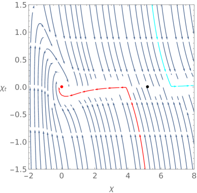
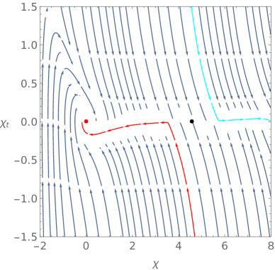
Figure 1: The $\chi_{t}\times\chi$ graphs considering phase space cuts $\left(\chi,\lambda,\chi_{t},\lambda_{t}\right)$ fixing $\lambda_{t}=\lambda_{tt}=0$ and $\beta_{0}=0.001$ with $\left(\lambda,\alpha_{0}\right)=\left(173,0.0001\right)$ (top graph) and $\left(\lambda,\alpha_{0}\right)=\left(94,0.00034\right)$ (bottom graph). The red and black points correspond to the critical points $P_{0}$ and $P_{c}$, respectively. For $\alpha_{0}=0.0001$, we have $P_{c}=\left(5.18,173,0,0\right)$ and for $\alpha_{0}=0.00034$, we have $P_{c}=\left(4.58,94,0,0\right)$. The red (cyan) trajectories represent trajectories that, when reaching the attractor line close to $\dot{\chi}=0$, approach (depart) from the origin. Details on the interpretation of the graphics are presented in the body of the text.                 

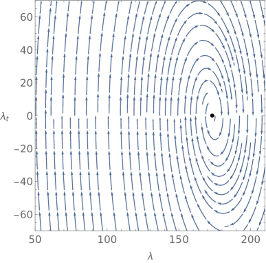
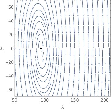
Figure 2: The $\lambda_{t}\times\lambda$ graphs considering phase space cuts $\left(\chi,\chi_{t},\lambda\text{,}\lambda_{t}\right)$ setting $\chi_{t}=0$ and $\beta_{0}=0.001$ with $\left(\chi,\alpha_{0}\right)=\left(5.18,0.0001\right)$ and (top graph) and $\left(\chi,\alpha_{0}\right)=\left(4.58,0.00034\right)$ (bottom graph). The black points correspond to the critical points $P_{c}=\left(5.18,173,0,0\right)$ (top graph) and $P_{c}=\left(4.58,94,0,0\right)$ (bottom graph). Details on the interpretation of the graphics are presented in the body of the text.             

The first (and most relevant) point that can be seen in figure 1 is that there is an attractor line close to $\chi_{t}\simeq 0$. The existence of this region is consistent with any value of $\alpha_{0}<10^{-3}$ and $\beta_{0}<3\times 10^{-2}$ and for any interval of $\lambda_{t}$ and $\lambda_{tt}$ that yields real results in the region of interest $\chi\in[0,8]$. At the same time that the $\chi$ field tends to the attracting line ($\chi_{t}\simeq 0$), figure 2 indicates that $\lambda$ tends to a finite value and $\lambda_{t}\rightarrow 0$. This finite value of $\lambda$ essentially depends on the value of $\chi$ with variations on a smaller scale due to changes in the parameter $\alpha_{0}$. The other fixed parameters $\chi_{t}$ and $\beta_{0}$ in figure 2 change how $\lambda$ approaches the accumulation point but does not change its value. We will see in the Sec. III.2 that this attractor region in the $4$-dimensional phase space where $\left(\chi,\lambda,\chi_{t}\text{,}\lambda_{t}\right)\simeq\left(\chi,\lambda\left(\chi\right),0,0\right)$ corresponds to a slow-roll inflationary regime.

Once the attractor region is reached, we must ask ourselves if inflation occurs enough, i.e., if it generates a sufficient number of $e$-folds and if it ends in a reheating phase. The answer to this question essentially depends on the position where the $\chi$ field hits the attractor line in figure 1. If the $\chi$ field is to the left of the critical point $P_{c}$ (black dots in the graphs of figure 1), inflation proceeds normally and ends in a phase of coherent oscillations associated with the beginning of reheating. On the other hand, if $\chi$ is to the right of $P_{c}$ the value of $\chi$ increases indefinitely, and inflation never ends (see Ref. [44] for details). Thus, a physical inflationary regime, i.e., consistent with a graceful exit, only occurs if $\chi<\chi_{c}\Rightarrow\alpha_{0}<3\left(e^{\chi}-4\right)^{-2}$ which for sufficiently large $\chi$ corresponds to $\alpha_{0}<3e^{-2\chi}$.

In the next section, we will see how to describe the dynamics of the $\chi$ and $\lambda$ fields during the slow-roll inflationary phase.

III.2 Inflation in the slow-roll leading order regime

This section aims to describe the dynamics of $\chi$, $\lambda$, and their derivatives during the inflationary regime considering the slow-roll approximation. In the region associated with physical inflation, the parameter $\chi$ is a monotonic decreasing function of time, so we can parameterize the various quantities in terms of $\chi$. For the case of Starobinsky model, we know that in the slow-roll leading order regime $\chi_{t}\sim\delta$ and $\chi_{tt}\sim\delta^{2}$, where $\delta$ is the slow-roll factor defined as $\delta\equiv e^{-\chi}$. And for Starobinsky plus $R^{3}$ model (i.e., $\beta_{0}=0$ and $\alpha_{0}\neq 0$), we have [44]

$$\chi_{t}\sim\left(\delta-\frac{\alpha_{0}}{3}\delta^{-1}\right).$$ (33)

Note that since $\alpha_{0}<3\delta^{2}$, the second term of the previous expression is of the same order or less than $\delta$.

The previous discussion allows us to associate the factor $\delta$ as a parameter that controls the slow-roll approximation order, i.e., a quantity $f\sim\delta^{n}$ will be an $n$th-order slow-roll quantity. In this case, $\chi_{t}$ present in (33) is first-order in slow-roll, since both $\delta$ and $\alpha_{0}\delta^{-1}$ are first-order. To apply this reasoning in our model, it is also necessary to establish what is the maximum slow-roll order of the parameter $\beta_{0}$. A more detailed analysis of the field equations in the attractor region shows us that, for slow-roll inflation, $\beta_{0}\lesssim\delta$, i.e., $\beta_{0}$ is a (at most) first-order slow-roll parameter (for details see Ref. [58]).

Once the slow-roll (maximum) orders of the parameters $\alpha_{0}$ and $\beta_{0}$ are known, we can propose the following ansatz for $\chi_{t}$:

$$\chi_{t}\simeq c_{1}\delta+\beta_{0}\sum\limits_{n=0}^{\infty}b_{n}\left(\beta_{0}\delta^{-1}\right)^{n}+\alpha_{0}\delta^{-1}\sum\limits_{n=0}^{\infty}d_{n}\left(\beta_{0}\delta^{-1}\right)^{n}.$$ (34)

This ansatz has the following properties:

• All terms are first-order in slow-roll, this being the leading order of $\chi_{t}$;

• In the limit of $\beta_{0}\rightarrow 0$, we recover the result (33);

• Derivating Eq. (34) with respect to $t$, we increase the slow-roll order, i.e., $\chi_{tt}$ is second order, $\chi_{ttt}$ is third order, etc.

By following similar reasoning, we propose the following ansatz for $\lambda$:

$$\lambda\simeq\delta^{-1}+\sum\limits_{n=0}^{\infty}g_{n}\left(\beta_{0}\delta^{-1}\right)^{n}+\alpha_{0}\delta^{-2}\sum_{n=0}^{\infty}j_{n}\left(\beta_{0}\delta^{-1}\right)^{n}.$$ (35)

In this case, the first term is of order $\mathcal{O}\left(-1\right)$ in slow-roll, and the others are zero-order terms. The $\mathcal{O}\left(-1\right)$ order term is necessary as we know that in the case of Starobinsky $\lambda=\delta^{-1}-1$ (see Eq. (19) with $\alpha_{0}=\beta_{0}=0$). Analogously to $\chi_{t}$, each derivative of $\lambda$ with respect to $t$ increases by one the slow-roll order.

The next step is substituting these two ansatzes and their derivatives into Eqs. (16), (18), and (19) taking into account only the slow-roll leading order. In this situation, we get

$$3h\chi_{t}-\frac{1}{3}\delta\lambda\left(1-\delta\lambda-2\delta-\frac{2}{3}\alpha_{0}\delta\lambda^{2}\right) \simeq 0,$$ (36)

$$3\beta_{0}h\lambda_{t}-\left[1-\delta\left(1+\lambda+\alpha_{0}\lambda^{2}\right)\right] \simeq 0,$$ (37)

where

$$h^{2}\simeq\frac{1}{6}\delta\lambda\left(1-\frac{1}{2}\delta\lambda\right).$$ (38)

By explicitly substituting Eqs. (34) and (35) in these last three expressions, we get after a long calculation

$$\chi_{t}\simeq-\frac{2\sqrt{3}}{3\left(3-\beta_{0}\delta^{-1}\right)}\delta\left(1-\frac{\alpha_{0}}{3}\delta^{-2}\right),$$ (39)

$$\lambda\simeq\delta^{-1}-\frac{3-2\beta_{0}\delta^{-1}}{3-\beta_{0}\delta^{-1}}-\alpha_{0}\delta^{-2}\left(1+\frac{\frac{1}{3}\beta_{0}\delta^{-1}}{3-\beta_{0}\delta^{-1}}\right),$$ (40)

with

$$h^{2}\simeq\frac{1}{12}\left(1-2\delta-\frac{2}{3}\alpha_{0}\delta^{-1}\right).$$ (41)

For details see appendix A. It is worth noting that the previous expressions are well defined only for $\beta_{0}\delta^{-1}<3$. Note in Eq. (39) the existence of two terms that, in the slow-roll leading order, are first-order terms. In Eq. (40), we have the $\mathcal{O}\left(-1\right)$ order term in addition to the zero-order corrections. Finally, $h^{2}$, related to the Hubble parameter, is given by the zero-order slow-roll leading term plus first-order corrections (independent of $\beta_{0}$).

III.2.1 Calculation of slow-roll parameters and number of $e$-folds

The characterization of the inflationary regime is done through the slow-roll parameters

$$\epsilon\equiv-\frac{\dot{H}}{H^{2}}=-\frac{h_{t}}{h^{2}},$$ (42)

$$\eta\equiv-\frac{1}{H}\frac{\dot{\epsilon}}{\epsilon}=-\frac{1}{h}\frac{\epsilon_{t}}{\epsilon}.$$ (43)

By substituting (39) and (40) in (17), we get

$$h_{t}\simeq-\frac{\delta^{2}}{3\left(3-\beta_{0}\delta^{-1}\right)}\left(1-\frac{\alpha_{0}}{3}\delta^{-2}\right)^{2}.$$

Thus, in the slow-roll leading order, we have

$$\epsilon\simeq\frac{4\delta^{2}}{\left(3-\beta_{0}\delta^{-1}\right)}\left(1-\frac{\alpha_{0}}{3}\delta^{-2}\right)^{2}.$$ (44)

The next step is calculating $\eta$. Differentiating $\epsilon$ and using this result together with $\epsilon$ itself in Eq. (43), we get

$$\eta\simeq-\frac{4\delta}{\left(3-\beta_{0}\delta^{-1}\right)^{2}}\left[3\left(2-\beta_{0}\delta^{-1}\right)+\alpha_{0}\delta^{-2}\left(2-\frac{1}{3}\beta_{0}\delta^{-1}\right)\right].$$ (45)

Note that by construction $\alpha_{0}\delta^{-2}<3$ and $\beta_{0}\delta^{-1}<3$.

In order to have robust inflation, i.e., with enough number of e-folds, we must have $\epsilon\ll 1$ and $\eta\ll 1$. Thus, from the equations (44) and (45), we see that this occurs for $\delta\ll 1$ (typically $\chi\gtrsim 4$). However, unlike the Starobinsky case, we also have lower bounds for $\delta$. In fact, the slow-roll inflationary regime only occurs if

$$\delta>\frac{\beta_{0}}{3}\text{ \ and \ }\delta>\sqrt{\frac{\alpha_{0}}{3}}.$$ (46)

The first condition does not represent a real difficulty for the existence of slow-roll inflation, because even if at some point we have $\delta<\beta_{0}$, the dynamics of the phase space guarantees that $\chi$ decreases monotonically so that at some point $\delta$ becomes greater than $\beta_{0}$ (see figure 1). The second condition represents a real constraint for carrying out a physical inflation (see discussion at the end of Sec. III.1). For a discussion of the implications of this second constraint and the initial conditions of inflation see Ref. [44].

Next we will calculate the number of $e$-folds $N$ in the slow-roll leading order. By the definition of $N$, we have

$$N=\int_{t}^{t_{e}}Hdt\simeq\frac{1}{4}\int_{\delta}^{\delta_{e}}\frac{\left(1-2\delta-\frac{2}{3}\alpha_{0}\delta^{-1}\right)\left(3-\beta_{0}\delta^{-1}\right)}{\delta^{2}\left(1-\frac{\alpha_{0}}{3}\delta^{-2}\right)}d\delta,$$

where the index $e$ corresponds to the end of inflation. To integrate this expression, it is convenient to perform the following change of variable:

$$x=\frac{\delta_{m}}{\delta}\text{ \ where }\delta_{m}=\sqrt{\frac{\alpha_{0}}{3}}.$$ (47)

In this case, we get

$$N\simeq-\frac{1}{4\delta_{m}}\int_{x}^{x_{e}}\frac{\left(x-2\delta_{m}-2x^{2}\delta_{m}\right)\left(3-\beta_{0}\delta_{m}^{-1}x\right)}{1-x^{2}}\frac{dx}{x},$$

whose solution is

$$N\simeq-\frac{1}{4\delta_{m}}\left\{-2x\beta_{0}-6\delta_{m}\ln x+\right.$$

$$\left.+\frac{\beta_{0}+12\delta_{m}^{2}}{2\delta_{m}}\ln\left[\left(1-x\right)\left(1+x\right)\right]+\frac{3+4\beta_{0}}{2}\ln\left(\frac{1+x}{1-x}\right)\right\}_{x}^{x_{e}}.$$

By considering only leading terms and taking into account that $x_{e}\ll x$, we finally get

$$N\simeq\frac{3}{8}\sqrt{\frac{3}{\alpha_{0}}}\ln\left[\left(1-x\right)^{\gamma-1}\left(1+x\right)^{\gamma+1}\right]\text{ \ where \ }\gamma^{2}=\frac{\beta_{0}^{2}}{3\alpha_{0}}\text{.\ }$$ (48)

By construction, physical inflation occurs in the interval $0\leq x<1$. In fact, when $x\rightarrow 1$ we have $\delta\rightarrow\delta_{m}$ which corresponds approximately to $\chi\rightarrow\chi_{c}$ (see eq. (25)). However, the expression (48) has an extra restriction due to the presence of the $\beta_{0}$ term. For $\beta_{0}^{2}>3\alpha_{0}\Rightarrow\gamma>1$, we have that when $x\rightarrow 1$, the value of $N$ diverges to $-\infty$, and this is clearly not physical. What happens is that for $\gamma>1$, the function $N$ presents a maximum point within the interval $0\leq x<1$. Differentiating $N$ with respect to time, we have

$$N_{t}\simeq\frac{3x}{8}\sqrt{\frac{3}{\alpha_{0}}}\left[\frac{-\left(\gamma-1\right)\left(1+x\right)+\left(\gamma+1\right)\left(1-x\right)}{\left(1-x\right)\left(1+x\right)}\right]\chi_{t}.$$

So, for $\gamma>1$, we have

$$N_{t} = 0\Rightarrow-\left(\gamma-1\right)\left(1+x_{\max}\right)+\left(\gamma+1\right)\left(1-x_{\max}\right)=0$$ (49)

$$\Rightarrow x_{\max}=\frac{1}{\gamma}<1\text{.}$$

On the other hand, for values of $x$ such that $x_{\max}\leq x<1$, we get

$$\beta_{0}\delta^{-1}=3\gamma x\geq 3\Rightarrow\delta\leq\frac{\beta_{0}}{3}$$

which violates the first condition of Eq. (46).

Therefore, based on the previous analysis, we conclude that Eqs. (44), (45) and (48) referring to the quantities $\epsilon$, $\eta$ and $N$ are valid in the following intervals:

$$\left\{\begin{array}[]{c}\gamma\leq 1\Rightarrow x<1\Rightarrow\chi<\ln\left(\sqrt{\frac{3}{\alpha_{0}}}\right)\\ \gamma>1\Rightarrow x<x_{\max}\Rightarrow\chi<\ln\left(\frac{3}{\beta_{0}}\right)\end{array}\right..$$ (50)

In the next section, we will study the inflationary regime from the perturbative point of view.

IV Inflation via cosmological perturbation theory

In this section, we investigate inflation of the model (2) via cosmological perturbations. Recall that its background dynamic equations are the Friedmann ones, given by Eqs. (12) and (13), and the equations of motion for the scalar fields $\chi$ and $\lambda$, given by Eqs. (14) and (15).

Before proceeding with our developments, it is worth commenting on scalar perturbations. In addition to the perturbations of the two scalar fields, which we will denote by $\delta\chi$ and $\delta\lambda$, we have the scalar perturbations of the metric. The line element in the perturbed Friedmann-Lemaître-Robertson-Walker (FLRW) metric is given by

$$ds^{2} = -\left(1+2A\right)dt^{2}+2a\partial_{i}Bdx^{i}dt+$$ (51)

$$+a^{2}\left[\left(1-2\psi\right)\delta_{ij}+2\partial_{ij}E+h_{ij}\right]dx^{i}dx^{j},$$

with $A$, $B$, $\psi$ and $E$ being the scalar perturbations of the metric [67, 68]. In order to obtain the perturbative field equations through a perturbation directly in the action, we need to write it up to the second order in the perturbations. In this case, we must consider second-order terms for perturbations involving only scalar field perturbations (e.g., $\delta\chi^{2}$), second-order terms involving only metric scalar perturbations (e.g., $A^{2}$) and cross terms, that is, a product of first-order terms (e.g., $A\delta\chi$). In the following subsection, by following a perturbative procedure directly in the action, along the lines of that found in Refs. [69, 70, 68], and assuming the spatially flat gauge, we obtain and discuss the equations of motion for the perturbations.

IV.1 Equations for scalar perturbations

The first step in order to perturbate the action is defining the perturbations of the scalar fields. For an inhomogeneous distribution of matter, we write

$$\chi\left(t,x\right) =\chi\left(t\right)+\delta\chi\left(t,x\right),$$ (52)

$$\lambda\left(t,x\right) =\lambda\left(t\right)+\delta\lambda\left(t,x\right).$$ (53)

In turn, the metric in Eq. (51) is written as

$$g^{\rho\sigma}\left(t,x\right)=g^{\rho\sigma}\left(t\right)+\delta g^{\rho\sigma}\left(t,x\right).$$ (54)

By writing Eq. (2) up to the second order in the perturbations and taking their variations with respect to each one of the perturbations, we are able to obtain the following equations of motion for the perturbations $\delta\chi$ and $\delta\lambda$

$$\delta\ddot{\chi}+3H\delta\dot{\chi}-\frac{1}{a^{2}}\nabla^{2}\left(\delta\chi\right)+$$

$$+\frac{\beta_{0}}{6}e^{-\chi}\dot{\lambda}\left(\dot{\lambda}\delta\chi-2\delta\dot{\lambda}\right)+V_{\chi\chi}\delta\chi+V_{\chi\lambda}\delta\lambda=$$

$$\dot{\chi}\dot{A}+\frac{1}{a}\dot{\chi}\nabla^{2}B-2V_{\chi}A,$$ (55)

and

$$\beta_{0}e^{-\chi}\left[\delta\ddot{\lambda}+\left(3H-\dot{\chi}\right)\delta\dot{\lambda}-\frac{1}{a^{2}}\nabla^{2}\left(\delta\lambda\right)+\right.$$

$$\left.-\dot{\lambda}\delta\dot{\chi}-3V_{\lambda}\delta\chi\right]-3\left(V_{\chi\lambda}\delta\chi+V_{\lambda\lambda}\delta\lambda\right)=$$

$$\beta_{0}e^{-\chi}\left(\dot{\lambda}\dot{A}+\dot{\lambda}\frac{1}{a}\nabla^{2}B+\dot{\chi}\dot{\lambda}A\right)+6V_{\lambda}A,$$ (56)

as well as the Einstein equations

$$H\left(3HA-\frac{k^{2}}{a}B\right)=-\frac{1}{4}\left[3\dot{\chi}\delta\dot{\chi}-\beta_{0}e^{-\chi}\dot{\lambda}\delta\dot{\lambda}+\right.$$

$$\left.-\left(3\dot{\chi}^{2}-\beta_{0}e^{-\chi}\dot{\lambda}^{2}\right)A+\frac{1}{2}\beta_{0}e^{-\chi}\dot{\lambda}^{2}\delta\chi+V_{\chi}\delta\chi+V_{\lambda}\delta\lambda\right],$$ (57)

and

$$HA=\frac{1}{4}\left(3\dot{\chi}\delta\chi-\beta_{0}e^{-\chi}\dot{\lambda}\delta\lambda\right).$$ (58)

The double subscript in potential $V$ represents second-order differentiation with respect to the corresponding scalar fields.

IV.2 Equations in the slow-roll leading order regime

Once we obtain Eqs. (55), (56), (57) and (58), which completely describe the evolution of scalar perturbations, the next step is to write them in the slow-roll leading order regime. This is not a trivial task and therefore, we will initially present the particular case of the Starobinsky model ($\alpha_{0}=\beta_{0}=0$). In this case, Eqs. (55), (56), (57) and (58) reduce to

$$\delta\ddot{\chi}+3H\delta\dot{\chi}-\frac{1}{a^{2}}\nabla^{2}\left(\delta\chi\right)+\hat{V}_{\chi\chi}\delta\chi+\hat{V}_{\chi\lambda}\delta\lambda=$$

$$\dot{\chi}\dot{A}+\frac{1}{a}\dot{\chi}\nabla^{2}B-2\hat{V}_{\chi}A,$$ (59)

$$\hat{V}_{\chi\lambda}\delta\chi+\hat{V}_{\lambda\lambda}\delta\lambda=-2\hat{V}_{\lambda}A,$$ (60)

$$H\left(3HA-\frac{k^{2}}{a}B\right)=-\frac{1}{4}\left(3\dot{\chi}\delta\dot{\chi}-3\dot{\chi}^{2}A+\hat{V}_{\chi}\delta\chi+\hat{V}_{\lambda}\delta\lambda\right)$$ (61)

and

$$HA=\frac{3}{4}\dot{\chi}\delta\chi,$$ (62)

with

$$\hat{V}\left(\chi,\lambda\right)=\frac{1}{3}\kappa_{0}e^{-2\chi}\lambda\left(e^{\chi}-1-\frac{1}{2}\lambda\right).$$ (63)

In Sec. III.2, we saw, in the context of the background, the behavior of the scalar fields, their derivatives and the relationships they keep between them. Once the slow-roll factor $\delta$ was established, we recall that in the slow-roll leading order regime, we obtain

$$\dot{\chi}\sim\delta\text{, \ }\lambda\sim\delta^{-1}\text{, \ }H\sim\delta^{0}\text{, \ }\beta_{0}\sim\delta\text{ \ and \ }\alpha_{0}\sim\delta^{2}\,\text{,}$$

and that with each differentiation with respect to time in the scalar fields, an order of slow-roll is increased, that is, $\ddot{\chi}\sim\delta^{2}$ and $\dot{\lambda}\sim\delta^{0}$. By making the constructions in this section, some assumption is necessary, namely, to find the slow-roll orders of the perturbations, we need to establish the slow-roll order of one of them. In this sense, we take the perturbation $\delta\chi$ as a zero-order slow-roll quantity. Also, we keep in mind that derivatives do not change the slow-roll order of perturbations. We are now able to write the equations of motion in the slow-roll leading order. Analyzing Eq. (62), note that since $\dot{\chi}\delta\chi\sim\delta$, perturbation $A$ must be at most first-order in slow-roll. Regarding Eq. (61), in its right member, we have the first and third terms, which are of first-order, the second term, which is subdominant $3\dot{\chi}^{2}A$ of third-order in slow-roll, and the last one is null, since $\hat{V}_{\lambda}=0$. Furthermore, since in its left member we have $3H^{2}A\sim\delta$, we conclude that perturbation $B$ is at most first-order in slow-roll. In turn, as $\hat{V}_{\chi\lambda}\sim\delta$ and $\hat{V}_{\lambda\lambda}\sim\delta^{2}$, we see that Eq. (60) establish the perturbation leading order of $\delta\lambda$, namely, $\delta\lambda\sim\delta^{-1}$. With Eq. (60), we can still write $\delta\lambda$ in terms of $\delta\chi$ and substitute in Eq. (59). Thus, on the left side of Eq. (59), the first three terms are of zero order in slow-roll, while all other terms of the equation give us subdominant contributions. So we can write

$$\delta\ddot{\chi}+3H\delta\dot{\chi}-\frac{1}{a^{2}}\nabla^{2}\left(\delta\chi\right)\simeq 0.$$ (64)

When developing the previous analysis now for the case of the complete equations, we find that the perturbations evolve, in the slow-roll leading order regime, with the same orders obtained previously. In short, the scalar perturbations evolve in the form $A\sim B\sim\delta$ and $\delta\lambda\sim\delta^{-1}$. It is interesting to note that the perturbation $\delta\lambda$ goes in leading order regime with $\delta^{-1}$, and that if it were otherwise, it would seriously compromise the slow-roll dynamics.

By applying all the discussion raised above, we find, in the slow-roll leading order regime, the following equations of motion for the perturbations of the scalar fields

$$\delta\ddot{\chi}+3H\delta\dot{\chi}-\frac{1}{a^{2}}\nabla^{2}\left(\delta\chi\right)\simeq\frac{1}{3}\kappa_{0}\left(\delta\chi-e^{-\chi}\delta\lambda\right),$$ (65)

and

$$\beta_{0}\left[\delta\ddot{\lambda}+3H\delta\dot{\lambda}-\frac{1}{a^{2}}\nabla^{2}\left(\delta\lambda\right)\right]\simeq\kappa_{0}\left(\delta\chi-e^{-\chi}\delta\lambda\right).$$ (66)

These results are in agreement with those obtained in Ref. [58], where the Starobinsky$+R\square R$ model is explored.

IV.3 Adiabatic and isocurvature perturbations

In this subsection, we define adiabatic and isocurvature perturbations, obtain expressions that describe their dynamics, and study their solutions.

The action (2) can be rewritten, along the lines of Ref. [71], compactly as

$$S=\frac{M_{Pl}^{2}}{2}\int d^{4}x\sqrt{-g}\left(-\frac{1}{2}g^{\mu\nu}G_{IJ}\left(\Phi\right)\partial_{\mu}\Phi^{I}\partial_{\nu}\Phi^{J}-3V\right),$$ (67)

where the scalars $\Phi^{I}\left(x\right)$ are seen as local coordinates of the scalar field space with metric $G_{IJ}\left(\Phi\right)$

$$\Phi^{I}=\begin{pmatrix}\chi\\ \lambda\end{pmatrix},\text{ \ }G_{IJ}\left(\Phi\right)=\begin{pmatrix}3&0\\ 0&-\beta_{0}e^{-\chi}\end{pmatrix},$$ (68)

and $V$ represents the potential of the model, Eq. (3). In a two-field scalar model, the field space is $2$-dimensional and characterized by $G_{IJ}\left(\Phi\right)$. To conveniently describe the evolution of perturbations, we can define a basis having a tangent direction, which we will denote by $\hat{\sigma}^{I}$, and another orthogonal, $\hat{s}^{I}$, to the background trajectories. Tangent directions to background trajectories are associated with adiabatic perturbation, while orthogonal directions are associated with isocurvature perturbation. In this sense, we build the basis through the definitions, respectively, of the module of the velocity vector, the unit velocity vector in the tangent direction and the normalization rule

$$\dot{\sigma}=\sqrt{G_{IJ}\dot{\Phi}^{I}\dot{\Phi}^{J}},\text{\ \ }\hat{\sigma}^{I}=\frac{\dot{\Phi}^{I}}{\dot{\sigma}}\text{ \ and \ }G_{IJ}\hat{\sigma}^{I}\hat{\sigma}^{J}=1,$$ (69)

and for the orthogonal direction, the normalization and orthogonality rules

$$G_{IJ}\hat{s}^{I}\hat{s}^{J}=-1\text{ \ and \ }G_{IJ}\hat{s}^{I}\hat{\sigma}^{J}=0.$$ (70)

For our case, we have for the velocity module $\dot{\sigma}$

$$\dot{\sigma}=\sqrt{3\dot{\chi}^{2}-\beta_{0}e^{-\chi}\dot{\lambda}^{2}}.$$ (71)

Note that it is directly related to the Friedmann equation (13). For the unit velocity vectors, we write

$$\hat{\sigma}^{\chi}=\frac{\dot{\chi}}{\dot{\sigma}}\text{ \ and \ }\hat{\sigma}^{\lambda}=\frac{\dot{\lambda}}{\dot{\sigma}}.$$ (72)

In turn, for the unit vectors in the orthogonal direction to the background trajectories, we have

$$\hat{s}^{\chi}=\sqrt{\frac{\beta_{0}e^{-\chi}}{3}}\frac{\dot{\lambda}}{\dot{\sigma}}\text{ \ and \ }\hat{s}^{\lambda}=\sqrt{\frac{3}{\beta_{0}e^{-\chi}}}\frac{\dot{\chi}}{\dot{\sigma}}.$$ (73)

Continuing our study on the evolution of scalar perturbations, we point out that the quantity $\delta\Phi_{g}^{I}$ given by

$$\delta\Phi_{g}^{I}=\delta\Phi^{I}+\frac{\dot{\Phi}^{I}}{H}\psi,$$ (74)

is gauge invariant. It turns out that $\psi=0$ when working on a spatially flat gauge, so that $\delta\Phi_{g}^{I}=\delta\Phi^{I}$. That said, by projecting $\delta\Phi^{I}$ in the $\hat{\sigma}$ and $\hat{s}$ directions, we construct the adiabatic $Q_{\sigma}$ and isocurvature $Q_{s}$ perturbations, respectively. In that sense, we have

$$Q_{\sigma}=\hat{\sigma}^{J}G_{IJ}\delta\Phi^{I}=\frac{3\dot{\chi}\delta\chi-\beta_{0}e^{-\chi}\dot{\lambda}\delta\lambda}{\dot{\sigma}},$$ (75)

and

$$Q_{s}=\hat{s}^{J}G_{IJ}\delta\Phi^{I}=\frac{\sqrt{3\beta_{0}e^{-\chi}}\left(\dot{\lambda}\delta\chi-\dot{\chi}\delta\lambda\right)}{\dot{\sigma}}.$$ (76)

It is worth noting that from the point of view of the slow-roll approximation both Eq. (75) and Eq. (76) are zero-order. By having written the expressions for the adiabatic and isocurvature perturbations, the next step is to invert the relations in order to obtain $\delta\Phi^{I}=\delta\Phi^{I}\left(Q\right)$. We obtain these relations by solving the linear system given by Eqs. (75) and (76). Thus, we find the expressions

$$\delta\chi=\frac{1}{\dot{\sigma}}\left(\dot{\chi}Q_{\sigma}-\sqrt{\frac{\beta_{0}e^{-\chi}}{3}}\dot{\lambda}Q_{s}\right),$$ (77)

and

$$\delta\lambda=\frac{1}{\dot{\sigma}}\left(\dot{\lambda}Q_{\sigma}-\sqrt{\frac{3}{\beta_{0}e^{-\chi}}}\dot{\chi}Q_{s}\right).$$ (78)

Once the field perturbations in terms of the adiabatic and isocurvature perturbations were obtained, we can write the second order perturbed action for $Q_{\sigma}$ and $Q_{s}$. Such an action is fundamentally constituted by quadratic terms involving $Q_{\sigma}$ and $Q_{s}$ (e.g., $Q_{\sigma}^{2}$), cross terms involving a $Q_{\sigma}$ or $Q_{s}$ and a metric perturbation (e.g., $AQ_{\sigma}$), and quadratic terms for metric perturbations (e.g., $A^{2}$). On the other hand, we can express the cross term only in terms of the perturbations $Q_{\sigma}$ and $Q_{s}$ by making use of the constraints from the Einstein equations, Eqs. (57) and (58). By taking these considerations into account, we find the following structure for the part of the action that depends only on $Q_{\sigma}$ and $Q_{s}$

$$S^{\left(2\right)}=\frac{M_{Pl}^{2}}{2}\int d^{4}x\sqrt{-g}\left(-\frac{1}{2}\partial_{\kappa}Q_{\sigma}\partial^{\kappa}Q_{\sigma}+\frac{1}{2}\partial_{\kappa}Q_{s}\partial^{\kappa}Q_{s}\right.+$$

$$+C_{Q_{\sigma}^{2}}Q_{\sigma}^{2}+C_{Q_{\sigma}Q_{s}}Q_{\sigma}Q_{s}+C_{Q_{s}^{2}}Q_{s}^{2}+$$

$$+\left.C_{Q_{\sigma}\dot{Q}_{\sigma}}Q_{\sigma}\dot{Q}_{\sigma}+C_{\dot{Q}_{\sigma}Q_{s}}\dot{Q}_{\sigma}Q_{s}+C_{Q_{\sigma}\dot{Q}_{s}}Q_{\sigma}\dot{Q}_{s}+C_{Q_{s}\dot{Q}_{s}}Q_{s}\dot{Q}_{s}\right),$$ (79)

where the coefficient of the cross kinetic term $\partial_{\kappa}Q_{\sigma}\partial^{\kappa}Q_{s}$ is zero, and the others can be found in Appendix B. It is interesting to analyze the behavior of kinetic terms and their possible contribution to the emergence of ghost-type instabilities. Note that the kinetic terms are canonical, equal and with reversed signs. This characteristic irremediably indicates that the existence of ghost-type instabilities is something intrinsic to the model and that it is essential to take this into account when performing the perturbation quantization process. Furthermore, the fact of the non-existence of the cross kinetic term is something expected and is directly related to our approach of making a consistent decomposition of the perturbations in the tangent and orthogonal directions to the trajectories of the background phase space.

When writing Eq. (79) considering a slow-roll leading order regime, we obtain

$$S^{\left(2\right)} \simeq \frac{M_{Pl}^{2}}{2}\int d^{4}x\sqrt{-g}\left\{-\frac{1}{2}\partial_{\kappa}Q_{\sigma}\partial^{\kappa}Q_{\sigma}+\frac{1}{2}\partial_{\kappa}Q_{s}\partial^{\kappa}Q_{s}+\right.$$ (80)

$$\left.-\frac{\kappa_{0}}{\dot{\sigma}^{2}}\left[1-\frac{1}{2}\left(\frac{3}{\beta_{0}e^{\chi}}+\frac{\beta_{0}e^{\chi}}{3}\right)\right]\dot{\chi}^{2}Q_{s}^{2}\right\}.$$

We now turn our attention to the task of writing the equations for the evolution of adiabatic and isocurvature perturbations. This is done by substituting the expressions (77) and (78) in the dynamic equations (65) and (66). In this case, taking the first derivatives of Eqs. (77) and (78), remembering that the background quantities can be considered constant, we are able to write

$$\ddot{Q}_{\sigma}+3H\dot{Q}_{\sigma}-\frac{1}{a^{2}}\nabla^{2}Q_{\sigma}\simeq 0,$$ (81)

and

$$\ddot{Q}_{s}+3H\dot{Q}_{s}+m^{2}Q_{s}\simeq 0,$$ (82)

where

$$m^{2}=-\left[\frac{1}{a^{2}}\nabla^{2}+\frac{\kappa_{0}}{3}\left(1-\frac{3}{\beta_{0}e^{\chi}}\right)\right].$$ (83)

Note that relations (81) and (82) indicate that the adiabatic $Q_{\sigma}$ and isocurvature $Q_{s}$ perturbations are decoupled, that is, they evolve independently in our model. That is an interesting result since such a decoupling usually does not occur. Generally, the isocurvature perturbation enter as source of the adiabatic one. [71].

From this point on, it becomes convenient to treat the field equations for the perturbations in a Mukhanov-Sasaki form. By making a redefinition of the perturbations and assuming conformal time and Fourier space, we get

$$\delta\varphi_{\sigma}^{\prime\prime}+\left(k^{2}-\frac{a^{\prime\prime}}{a}\right)\delta\varphi_{\sigma}\simeq 0,$$ (84)

$$\delta\varphi_{s}^{\prime\prime}+\left[k^{2}-\frac{a^{\prime\prime}}{a}-\frac{a^{2}\kappa_{0}}{3}\left(1-\frac{3}{\beta_{0}e^{\chi}}\right)\right]\delta\varphi_{s}\simeq 0,$$ (85)

with the prime representing derivative with respect to conformal time and where

$$\delta\varphi_{\sigma}\equiv aQ_{\sigma}\text{ \ and \ }\delta\varphi_{s}\equiv aQ_{s}\text{.}$$ (86)

In a de Sitter background (slow-roll zero order), we have

$$\frac{a^{\prime\prime}}{a}\simeq\frac{2}{\eta^{2}}\text{,\ \ }a\simeq-\frac{1}{H\eta}\text{\ \ and \ }H^{2}\simeq\frac{\kappa_{0}}{12}.$$ (87)

Furthermore, in the slow-roll zero order regime, we have

$$\dot{\chi}\simeq-\frac{1}{3}\frac{H^{-1}}{3-\beta_{0}\delta^{-1}}\delta\left(1-\frac{\alpha_{0}}{3}\delta^{-2}\right)\simeq 0\Rightarrow\chi=cte\text{.}$$ (88)

For consistency with several previous results, we have $\beta_{0}e^{\chi}<3$ so that we can define a quantity

$$M\equiv\frac{3}{\beta_{0}e^{\chi}}-1>0,$$ (89)

and in this way we write the expressions

$$\delta\varphi_{\sigma}^{\prime\prime}+k^{2}\left(1-\frac{2}{k^{2}\eta^{2}}\right)\delta\varphi_{\sigma}\simeq 0,$$ (90)

$$\delta\varphi_{s}^{\prime\prime}+k^{2}\left[1-\frac{2}{k^{2}\eta^{2}}\left(1-2M\right)\right]\delta\varphi_{s}\simeq 0.$$ (91)

Next, we will explore the solutions of Eqs. (90) and (91).

IV.4 Solutions to the perturbations

Once the equations for the dynamics of adiabatic and isocurvature perturbations have been established in the appropriate form, given by Eqs. (90) and (91), we can write and analyze their solutions.

In a subhorizon regime, $k\eta\gg 1$, equations to the perturbations are approximated by

$$\delta\varphi_{\sigma}^{\prime\prime}+k^{2}\delta\varphi_{\sigma}\simeq 0,\ \ k\eta\gg 1,$$

$$\delta\varphi_{s}^{\prime\prime}+k^{2}\delta\varphi_{s}\simeq 0,\text{ \ \ }k\eta\gg 1.$$

The quantization process in de Sitter takes the following initial conditions [72, 73]

$$\delta\varphi_{\sigma}\simeq\delta\varphi_{s}\simeq\frac{1}{\sqrt{2k}}e^{-ik\eta},\text{\ \ }k\eta\gg 1,$$ (92)

or

$$Q_{\sigma}\simeq Q_{s}\simeq\frac{1}{\sqrt{2k}a}e^{-ik\eta}\simeq-\frac{H\eta}{\sqrt{2k}}e^{-ik\eta}.$$ (93)

Note that due to the ghost-type behavior of isocurvature perturbation, the quantization of the $Q_{s}$ field was performed in the same way as in Refs. [74, 48]. In principle, this behavior can raise questions about the unitarity of the theory [75] (see also the discussions in Refs. [65, 66]). However, as we will see below, the $Q_{s}$ field decays rapidly after crossing the horizon, suppressing any observable effects associated with isocurvature perturbation.

The exact solution of Eqs. (90) and (91) can be written using a combination of Hankel’s functions as [73, 76]

$$\delta\varphi\left(\eta,k\right)=C_{1}\left(k\right)\sqrt{-\eta}H_{\nu}^{\left(1\right)}\left(-k\eta\right)+C_{2}\left(k\right)\sqrt{-\eta}H_{\nu}^{\left(2\right)}\left(-k\eta\right),$$ (94)

where for the adiabatic perturbation $\delta\varphi_{\sigma}$, we have $\nu_{\sigma}=3/2$, and for the isocurvature perturbation $\delta\varphi_{s}$, we have

$$\nu_{s}=\frac{3}{2}\sqrt{1-\frac{16M}{9}}.$$ (95)

To determine the constants, we compare the general solution with the initial conditions in Eq. (92). For the adiabatic case ($\nu_{\sigma}=3/2$) in the subhorizon regime, we find

$$C_{1\sigma}=-\frac{\sqrt{\pi}}{2}\text{ \ and \ }C_{2\sigma}=0,$$ (96)

so that

$$\delta\varphi_{\sigma}\left(\eta,k\right)=-\frac{\sqrt{-\pi\eta}}{2}H_{3/2}^{\left(1\right)}\left(-k\eta\right).$$ (97)

In turn, for the case of isocurvature perturbation, where $\nu_{s}$ is given by Eq. (95), for a subhorizon regime, we get

$$C_{1s}=\frac{\sqrt{\pi}}{2}e^{i\frac{\pi}{2}\left(\nu_{s}+\frac{1}{2}\right)}\text{ \ and \ }C_{2s}=0.$$ (98)

Thus, the solution to the isocurvature perturbation is written as

$$\delta\varphi_{s}\left(\eta,k\right)=\frac{\sqrt{-\pi\eta}}{2}e^{i\frac{\pi}{2}\left(\nu_{s}+\frac{1}{2}\right)}H_{\nu_{s}}^{\left(1\right)}\left(-k\eta\right).$$ (99)

Since the solutions (97) and (99) for the perturbations have been established, we can analyze their behavior in the superhorizon regime ($k\eta\ll 1$). Taking into account Eq. (87), which gives us the relation between $\eta$ and $a$ in a de Sitter background, for adiabatic perturbation, we find

$$\delta\varphi_{\sigma}\left(\eta,k\right)\simeq-\frac{i}{4\eta}\left(\frac{k}{2}\right)^{-3/2}\text{ \ or \ }Q_{\sigma}\simeq\frac{iH}{4}\left(\frac{k}{2}\right)^{-3/2},\text{ \ }k\eta\ll 1,$$ (100)

while for isocurvature perturbation, we have

$$\delta\varphi_{s}\left(\eta,k\right)\simeq-\frac{i\sqrt{\pi}e^{i\frac{\pi}{2}\left(\nu_{s}+\frac{1}{2}\right)}}{2\sin\left(\nu_{s}\pi\right)\Gamma\left(1-\nu_{s}\right)}\left(\frac{k}{2}\right)^{-\nu_{s}}\left(-\eta\right)^{\frac{1}{2}-\nu_{s}},\text{ \ }k\eta\ll 1,$$ (101)

or

$$Q_{s}\simeq-\frac{i\sqrt{\pi}e^{i\frac{\pi}{2}\left(\nu_{s}+\frac{1}{2}\right)}H^{\nu_{s}-\frac{1}{2}}}{2\sin\left(\nu_{s}\pi\right)\Gamma\left(1-\nu_{s}\right)}\left(\frac{k}{2}\right)^{-\nu_{s}}a^{\nu_{s}-\frac{3}{2}}.$$ (102)

The result in Eq. (100) tells us that the adiabatic perturbation is constant in the superhorizon limit, whereas Eq. (102) reveals a decaying behavior for the isocurvature one. Remembering that $M>0$, we have the following situations:

• If the quantity $\nu_{s}$ is real, we have

  $$0<M\leq\frac{9}{16}\Rightarrow 0\leq\nu_{s}<\frac{3}{2},$$ (103)

  representing a solution to $Q_{s}$ that decays with $a$.

• If the quantity $\nu_{s}$ is imaginary,

  $$M>\frac{9}{16}\Rightarrow\nu_{s}=i\frac{3}{2}\sqrt{\left|1-\frac{16M}{9}\right|},$$ (104)

  also providing a decaying solution, since we have the product of an oscillatory term and the term decaying with $a^{-\frac{3}{2}}$.

We can provide a quantitative measure of isocurvature perturbation by considering scales of interest during inflation (measured in CMB anisotropies). These ones are within the range $10^{-3}Mpc^{-1}<k<10^{4}Mpc^{-1}$, where the pivot scale is $k_{\ast}=0.002$ with $50<N_{\ast}<60$. The point is that during the inflationary regime, a given scale $k$ crosses the horizon at a specific value of the number of $e$-folds $N$. The smaller/larger the scale $k$ is, the smaller/larger the number of $e$-folds $N$ it experiences after crossing the horizon. Taking the smallest scale $k_{sm}=10^{4}Mpc^{-1}$, we find $N_{sm}=N_{\ast}-15.4$. In this sense, for $N_{\ast}=50$ and $\nu_{s}=1/2$, we get

$$Q_{s}\simeq\frac{1}{2}\left(\frac{k_{sm}}{2}\right)^{-\frac{1}{2}}e^{-N_{sm}}\sim 10^{-18},$$ (105)

which shows us that isocurvature perturbation is negligible after inflation. Since, in addition to this, they do not enter as a source of adiabatic perturbation, we can consider them negligible. All the previous analysis was carried out considering the slow-roll approximation.

In the next section, we will analyze the connection of our model with the observations.

V Observational constraints

At the end of the previous section, we show why isocurvature perturbation is negligible after inflation. Furthermore, since adiabatic perturbation has the same behavior as in the case of a single scalar field, we easily recognize the power spectrum and its connection with observational parameters. To make the connection with the observations, specifically to write the power spectrum, it is interesting to recover the mass units of the fields. In this sense, equations such as (12), (13), (69) and (75) need to be written in terms of massive fields given in Eq. (5). Since the curvature perturbation is given by $\mathcal{R=}\frac{H}{\dot{\sigma}}\left(\frac{\sqrt{2}}{M_{Pl}}Q_{\sigma}\right)$, the power spectrum of adiabatic perturbation is written as

$$\mathcal{P}_{\mathcal{R}}^{2}=\left.\frac{k^{3}}{2\pi^{2}}\left|\mathcal{R}\right|^{2}\right|_{k=Ha}=\left.\frac{1}{8\pi^{2}M_{Pl}^{2}}\frac{H^{2}}{\epsilon}\right|_{k=Ha},$$ (106)

where we evaluate it to $k=Ha$ at the instant when $k$ crosses the horizon. The result in Eq. (106) is identical to the power spectrum for single-field inflationary models. Thus, in the slow-roll leading order regime, the scalar spectral index $n_{s}$ and the tensor-to-scalar ratio $r$ are, respectively,

$$n_{s}=1+\eta-2\epsilon\text{ \ and \ }r=16\epsilon,$$ (107)

where $\epsilon$ and $\eta$ are the slow-roll parameters of the model given by the Eqs. (44) and (45). These equations depend on $\alpha_{0}$, $\beta_{0}$, and the number of $e$-folds $N$ through Eq. (48) which carries the dependency between $N$ and $\delta$.

In our paper, there are two types of Plots where we compare our model with observational data [40], built from Eq. (107) taking the three independent parameters $\alpha_{0}$, $\beta_{0}$, and $N$: the usual $n_{s}\times r_{0.002}$ plane and the parameter space $\alpha_{0}\times\beta_{0}$. The Plots are constructed by setting one of the parameters and varying the others. We use the range $52\leq N\leq 59$ for the number of inflation $e$-folds $N$ based on a reheating modeling. For details, see appendix C.

The figure 3 shows the $n_{s}\times r_{0.002}$ plane containing the observational constraints (in blue) obtained from Ref. [40] and the theoretical evolution of the model in two different situations.

In the top graph of figure 3, we fixed the parameter $\beta_{0}$ and varied the others. In it, the light red region represents Starobinsky$+R^{3}$ model, which starts at the light red points. In turn, the light yellow region represents the complete model with $\beta_{0}=1.5\times 10^{-2}$, starting at the yellow points. As we increase the values of the parameter $\alpha_{0}$, the region predicted by the model shifts to the left and slightly downwards, until it crosses the region of $95\%$ C.L.. This behavior can also be seen in Ref. [44], and it is consistent with the results obtained in Ref. [42], where $\beta_{0}=0$. These constraints establish, in the most conservative way, a maximum value for $\alpha_{0}\sim 10^{-4}$.

In the bottom graph of figure 3, on the other hand, we fixed the parameter $\alpha_{0}$ and varied the others. The light red region represents the Starobinsky$+R\square R$ model, which starts at the light red points. In turn, the light green region represents the complete model with $\alpha_{0}=10^{-5}$, starting at the light green points. As the values of $\beta_{0}$ increase, the region predicted by the model moves to the right and slightly upwards, until it crosses the region of $95\%$ C.L.. These constraints establish a maximum value for $\beta_{0}\sim 10^{-2}$. Similar results were obtained in Refs. [58, 59] for the Starobinsky$+R\square R$ case. However, a considerable difference between our results and those in Ref. [58] is checked for the constraint on the tensor-to-scalar ratio $r_{0.002}$. There, $r_{0.002}$ can assume larger values, so that the growth of the region predicted by the model is more accentuated. This difference is due to the fact that in Ref. [58], the definition for the curvature perturbation was not established properly by not making a separation of the background phase space trajectories in the tangent (adiabatic perturbation) and orthogonal (isocurvature perturbation) directions. On the other hand, our results are closer to those in Ref. [59], indicating that the approach of treating the $R\square R$ term as a small perturbation is relevant and consistent.

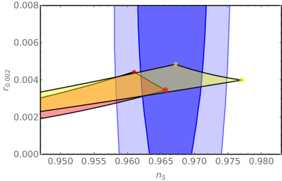
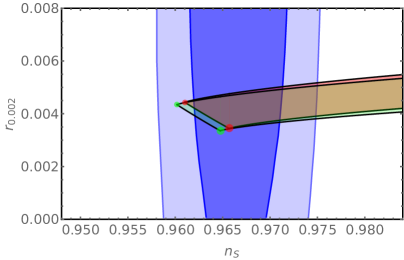
Figure 3: The contours in blue represent the constraints of the $n_{s}\times r_{0.002}$ plane in $68\%$ and $95\%$ C.L. due to observational data from Planck plus BICEP3/Keck plus BAO [40]. In the top graph, we set the parameter $\beta_{0}$ and vary the others. The light red circles represent Starobinsky$+R^{3}$ model for $N=52$ (smaller one) and $N=59$ (bigger one). The yellow circles represent the complete model with $\beta_{0}=1.5\times 10^{-2}$ for $N=52$ and $N=59$. As the values of $\alpha_{0}$ increase, the region predicted by the model shifts to the left and downwards, until it crosses the region of $95\%$ C.L.. When it crosses, the curves for Starobinsky$+R^{3}$ and the complete model with $\beta_{0}=1.5\times 10^{-2}$ for $N=52$ correspond to $\alpha_{0}=3.5\times 10^{-5}$ and $r_{0.002}=4.1\times 10^{-3}$ and $\alpha_{0}=4\times 10^{-5}$ and $r_{0.002}=4.1\times 10^{-3}$, respectively; for $N=59$ they correspond to $\alpha_{0}=8.2\times 10^{-5}$ and $r_{0.002}=2.8\times 10^{-3}$ and $\alpha_{0}=5.4\times 10^{-5}$ and $r_{0.002}=2.9\times 10^{-3}$, respectively. In the bottom graph, in turn, we set the parameter $\alpha_{0}$ and vary the others. The light red circles represent Starobinsky$+R\square R$ model for $N=52$ (smaller one) and $N=59$ (bigger one). The green circles represent the complete model with $\alpha_{0}=10^{-5}$ for $N=52$ and $N=59$. As the values of $\beta_{0}$ increase, the region predicted by the model shifts to the right and slightly upwards, until they cross the $95\%$ C.L. region. As it crosses, the curves for $N=52$ correspond approximately to $\beta_{0}=1.7\times 10^{-2}$ and $r_{0.002}=5.2\times 10^{-3}$; for $N=59$ they correspond approximately to $\beta_{0}=1.5\times 10^{-2}$ and $r_{0.002}=3.9\times 10^{-3}$.                     

Another plot developed, figure 4, is the parameter space $\alpha_{0}\times\beta_{0}$ allowed by the observations. In the top graph of figure 4, we have the Plot for $N=52$, while in the bottom graph of figure 4, we have it for $N=59$. The blue regions represent the allowed regions for the $\alpha_{0}$ and $\beta_{0}$ parameters in $68\%$ and $95\%$ C.L.. Note that the Plot for $N=52$ gives us a smaller region for the parameters if we compare it to the Plot for $N=59$. In addition, we can see two regions on each of the Plots. One is an approximated rectangular region completely within the $95\%$ C.L. (for $N=52$, the sides correspond to $\alpha_{0}=2.8\times 10^{-5}$ and $\beta_{0}=1.7\times 10^{-2}$, and for $N=59$, $\alpha_{0}=5.3\times 10^{-5}$ and $\beta_{0}=1.5\times 10^{-2}$), where the parameters $\alpha_{0}$ and $\beta_{0}$ do not keep a dependency between them, being able to assume any values independently. In this region of independence between the model parameters, we reproduced the results obtained in Refs. [42, 59] for each model separately. The other region is the asymptotic one for large values of $\alpha_{0}$ and $\beta_{0}$, whose occurrence suggests a dependence $\beta_{0}=\beta_{0}(\alpha_{0})$ between the parameters.

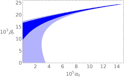
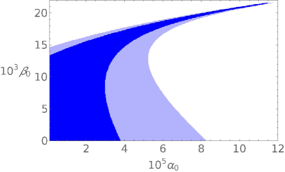
Figure 4: The regions in blue represent the allowed regions for the parameters $\alpha_{0}$ and $\beta_{0}$ in $68\%$ and $95\%$ C.L., due to observational data from Planck plus BICEP3/Keck plus BAO [40]. In the top graph we have the Plot for $N=52$, while in the bottom graph we have it for $N=59$. Note that the constraints for $N=59$ allow a larger region for the parameters $\alpha_{0}$ and $\beta_{0}$ in line with what we saw in the figure 3, whose predictions for $N=59$ are more within the region of $68\%$ C.L. Note that for large values of $\alpha_{0}$ and $\beta_{0}$, around $\alpha_{0}=1.5\times 10^{-4}$ and $\beta_{0}=2.5\times 10^{-2}$ ($N=52$) and $\alpha_{0}=2.2\times 10^{-4}$ and $\beta_{0}=1.2\times 10^{-2}$ ($N=59$), the predicted regions for the parameters converge to an asymptotic region. In this region, the values of $\alpha_{0}$ and $\beta_{0}$ suggest to keep a constraint.                         

VI Final comments

The Starobinsky model is one of the most competitive candidates for describing physical inflation. In addition to having a well-grounded theoretical motivation, it better fits the recent observations [39, 40]. Motivated by the success of such a model, we propose to investigate inflation based on the higher-order gravitational action characterized by the inclusion of all terms up to the second-order correction involving only the scalar curvature, namely, the terms $R^{2}$, $R^{3}$, and $R\square R$. In this sense, our proposed model has two additional dimensionless parameters, $\alpha_{0}$, and $\beta_{0}$, whose values represent deviations from Starobinsky.

Unlike Ref. [58], whose multi-field treatment used to address the term $R\square R$ gives us an inflation described by a scalar and a vector field, here, when passing from the original frame to the representation in the Einstein frame, the model is described through the dynamics of two scalar fields $\chi$ and $\lambda$, where only one of them is associated with a canonical kinetic term, and whose potential is $V\left(\chi,\lambda\right)$ given in Eq. (3). The study of inflation in a Friedmann background, through the analysis of the critical points and phase space of the model, is essential to verify the existence of an attractor region associated with the occurrence of an inflationary regime and to know if such a regime has a graceful exit. We took as a basis the study of particular cases developed in Refs. [58, 44], which deal with the Starobinsky$+R\square R$ and Starobinsky$+R^{3}$ extensions. We saw that there is an attractor line near $\chi_{t}\simeq 0$, corresponding to the slow-roll inflation, for any value of $\alpha_{0}<10^{-3}$ and $\beta_{0}<3\times 10^{-2}$. Furthermore, the occurrence of such a physical inflation regime essentially depends on the initial conditions for the $\chi$ field. If they are such that the $\chi$ field is to the right of the critical point $P_{c}$, the value of $\chi$ increases indefinitely, and inflation never ends. On the other hand, the occurrence of a consistent physical inflationary regime that has a graceful exit essentially requires that the initial conditions be such that $\chi<\chi_{c}$, i.e., that it is to the left of the critical point $P_{c}$. Finally, we conclude the background analysis with the study of inflation considering the slow-roll approximation. By defining the slow-roll factor $\delta$, which in our analysis is responsible for controlling the slow-roll approximation order, we obtain all relevant quantities, such as $\varepsilon$ and $\eta$, in the slow-roll leading order.

There is considerable literature about multi-field inflation models, which we took into account to develop the analysis at the perturbative level [70, 68]. The equations of motion for the scalar perturbations were obtained using the spatially flat gauge. By writing the equations in the slow-roll leading order approximation, we saw that the scalar perturbations of the metric are sub-dominant concerning the perturbations $\delta\chi$ and $\delta\lambda$. At this point, we performed a correct decomposition of the perturbations in the tangent (adiabatic perturbations) and orthogonal (isocurvature perturbations) directions to the phase space background trajectories. This way, adiabatic $Q_{\sigma}$ and isocurvature $Q_{s}$ perturbations are completely separated. Such a decomposition allows us to consistently establish the curvature perturbation, which led us to obtain observational constraints different from those obtained in Ref. [58]. The action written in terms of $Q_{\sigma}$ and $Q_{s}$ makes it clear that there are irremediably ghost-type instabilities in the model since the kinetic terms have opposite signs. Next, we write the equations of motion in a Mukhanov-Sasaki form in order to study their solutions. We obtained the exact solutions for the perturbations through a linear combination of the Hankel functions. Their analysis leads us to conclude that the isocurvature perturbation associated with the ghost field is negligible after inflation and that the adiabatic one has the same behavior as in the case of a single-field inflation. All previous results were obtained considering the slow-roll approximation. Thus, a question that remains is whether the suppression of isocurvature perturbation holds beyond the slow-roll regime. This issue will be addressed in a further work.

Finally, we confront our model with recent observations from the Planck satellite, BICEP3/Keck and BAO [39, 40], making use of a constraint on the number of $e$-folds $N$ of inflation ($52\leq N\leq 59$) based on reheating modeling [44]. For that, we made two types of Plots, namely, the usual $n_{s}\times r_{0.002}$ plane and the parameter space $\alpha_{0}\times\beta_{0}$. In this analysis, we have three parameters: $\alpha_{0}$, $\beta_{0}$, and $N$. Thus, to build the Plots, we set one of the parameters and vary the others. Fixing the parameter $\beta_{0}$, we observe that the region predicted by the model in the $n_{s}\times r_{0.002}$ plane shifts to the left and slightly downwards. On the other hand, fixing the parameter $\alpha_{0}$, we notice that the predicted region shifts to the right and slightly upwards. By setting $\alpha_{0}=0$, we get the Starobinsky$+R\square R$ model. In this context, we saw that inconsistency in establishing the curvature perturbation in Ref. [58] led them to obtain values higher than ours for the tensor-to-scalar ratio. In turn, by fixing the number of $e$-folds $N$, we construct the parameter space $\alpha_{0}\times\beta_{0}$ constrained by the observations. In general, the model predictions are more in agreement with the observations for a number of $e$-folds $N=59$. Our analysis, conservatively, restrict the parameters to maximum values of $\alpha_{0}\sim 10^{-4}$ and $\beta_{0}\sim 10^{-2}$. It is also worth pointing out the behavior of the $\alpha_{0}\times\beta_{0}$ parameter space. The $R^{3}$ and $R\square R$ terms are second-order correction terms on energy scales and, therefore, should contribute similarly to inflation. In this sense, the joint effect of such terms is reflected in the plot $\alpha_{0}\times\beta_{0}$. In fact, there is a considerable region in which the parameters do not depend on each other and which we can associate with the models separately discussed in Refs. [42, 44, 59, 58]. However, there is an asymptotic region for large values of $\alpha_{0}$ and $\beta_{0}$, where such parameters seem to keep a constraint. In this particular region, a change in one of the parameters necessarily implies a change in the other, so that the possibility of a dependence $\beta_{0}=\beta_{0}(\alpha_{0})$ is something to be investigated. This is a topic that the authors will address in a future research.

Appendix A Determination of $\chi_{t}$ and $\lambda$

The equations of motion of the model can be explicitly written in terms of the fields and their first derivatives as

$$\chi_{tt}+3h\chi_{t}-\frac{\beta_{0}}{6}e^{-\chi}\lambda_{t}{}^{2}+\frac{1}{3}e^{-2\chi}\lambda\left[\left(2-e^{\chi}\right)+\lambda+\frac{2}{3}\alpha_{0}\lambda^{2}\right]=0,$$ (108)

$$\beta_{0}\left[\lambda_{tt}-\left(\chi_{t}-3h\right)\lambda_{t}\right]-\left[1-e^{-\chi}\left(1+\lambda+\alpha_{0}\lambda^{2}\right)\right]=0,$$ (109)

where

$$h^{2}=\frac{1}{4}\chi_{t}^{2}-\frac{1}{12}\beta_{0}e^{-\chi}\lambda_{t}^{2}+\frac{1}{6}e^{-2\chi}\lambda\left[\left(e^{\chi}-1\right)-\frac{1}{2}\lambda-\frac{1}{3}\alpha_{0}\lambda^{2}\right].$$ (110)

By studying the case where the model parameters behave as $\beta_{0}\sim\delta\equiv e^{-\chi}$ and $\alpha_{0}\sim\delta^{2}$, we assume the quantities $\chi_{t}$ and $\lambda$ as follows, respectively,

$$\chi_{t}\simeq c_{1}\delta+\beta_{0}\sum\limits_{n=0}^{\infty}b_{n}\left(\beta_{0}\delta^{-1}\right)^{n}+\alpha_{0}\delta^{-1}\sum\limits_{n=0}^{\infty}d_{n}\left(\beta_{0}\delta^{-1}\right)^{n},$$ (111)

and

$$\lambda\simeq\delta^{-1}+\sum\limits_{n=0}^{\infty}g_{n}\left(\beta_{0}\delta^{-1}\right)^{n}+\alpha_{0}\delta^{-2}\sum_{n=0}^{\infty}j_{n}\left(\beta_{0}\delta^{-1}\right)^{n},$$ (112)

where we explore several possibilities of construction of the quantities $\chi_{t}$ (in first-order) and $\lambda$ (up to zero-order). In addition to the terms involving $\beta_{0}$ and $\alpha_{0}$ separately, we observe the need to introduce crossed terms due to the non-linearity of gravitation. We also notice fine limits when we take the particular cases $\alpha_{0}\rightarrow 0$ (Starobinsky$+R\square R$) and $\beta_{0}\rightarrow 0$ (Starobinsky+$R^{3}$).

By finding the coefficients of the series Eqs. (111) and (112), we substitute them in Eqs. (108) and (109) and solve the corresponding systems of equations. After a long calculation, we obtain that, for consistency with the Starobinsky case, $g_{0}\simeq-1$, as well as finding the following $n$th coefficients of the series

$$b_{n}\simeq-\frac{2}{3^{n+\frac{5}{2}}},\text{ for }n\geq 0,$$ (113)

$$d_{n}\simeq\frac{2}{3^{n+\frac{5}{2}}},\text{ for }n\geq 0,$$ (114)

$$g_{n}\simeq\frac{1}{3^{n}},\text{ for }n\geq 1,$$ (115)

$$j_{n}\simeq-\frac{1}{3^{n+1}},\text{ for }n\geq 1,$$ (116)

as well as

$$c_{1}\simeq-\frac{2}{3^{\frac{3}{2}}}\text{ \ and \ }j_{0}\simeq-1.$$ (117)

In possession of the $n$th coefficients, we can substitute them in the quantities $\chi_{t}$ and $\lambda$. In this case, for $\chi_{t}$,

$$\chi_{t}\simeq-\frac{2}{3^{\frac{3}{2}}}\delta\left[1+\frac{1}{3}\beta_{0}\delta^{-1}\sum\limits_{n=0}^{\infty}\left(\frac{\beta_{0}\delta^{-1}}{3}\right)^{n}-\frac{1}{3}\alpha_{0}\delta^{-2}\sum\limits_{n=0}^{\infty}\left(\frac{\beta_{0}\delta^{-1}}{3}\right)^{n}\right],$$ (118)

that converges with

$$\frac{\beta_{0}\delta^{-1}}{3}<1.$$ (119)

Thus,

$$\chi_{t}\simeq-\frac{2\sqrt{3}}{3}\frac{\delta}{3-\beta_{0}\delta^{-1}}\left(1-\frac{1}{3}\alpha_{0}\delta^{-2}\right).$$ (120)

In turn, for $\lambda$, we have

$$\lambda\simeq\delta^{-1}-\frac{3-2\beta_{0}\delta^{-1}}{3-\beta_{0}\delta^{-1}}-\alpha_{0}\delta^{-2}\left(1+\frac{\frac{1}{3}\beta_{0}\delta^{-1}}{3-\beta_{0}\delta^{-1}}\right).$$ (121)

The previous relation recovers the Starobinsky result

$$\lambda\simeq\delta^{-1}-1,$$ (122)

and Starobinsky+$R^{3}$, namely,

$$\lambda\simeq\delta^{-1}-1-\alpha_{0}\delta^{-2}.$$ (123)

Appendix B Coefficients in the action up to second-order for the perturbations $Q_{\sigma}$ and $Q_{s}$

In this appendix, we present the non-trivial coefficients in the second-order perturbed action for the adiabatic $Q_{\sigma}$ and isocurvature $Q_{s}$ perturbations, Eq. (79).

For $C_{Q_{\sigma}^{2}}$, we have

$$C_{Q_{\sigma}^{2}}=\left(\frac{1}{8\dot{\sigma}^{4}}\right)\left\{6\beta_{0}^{3}e^{-3\chi}\dot{\lambda}^{6}-55\beta_{0}^{2}e^{-2\chi}\dot{\lambda}^{4}\dot{\chi}^{2}-162\dot{\chi}^{6}\right.+$$

$$+\left.12\beta_{0}e^{-\chi}\left[-\dot{\chi}^{2}\ddot{\lambda}^{2}+2\dot{\lambda}\dot{\chi}\ddot{\lambda}\left(\dot{\chi}^{2}+\ddot{\chi}\right)+\dot{\lambda}^{2}\left(13\dot{\chi}^{4}-2\dot{\chi}^{2}\ddot{\chi}-\ddot{\chi}^{2}\right)\right]\right\}+$$

$$-\frac{1}{4}H^{-1}\left(\frac{4\kappa_{0}e^{-2\chi}}{9}\right)\left\{3\left[-1+e^{\chi}-\lambda\left(1+\alpha_{0}\lambda\right)\right]\dot{\lambda}+\lambda\left[6-3e^{\chi}+\lambda\left(3+2\alpha_{0}\lambda\right)\right]\dot{\chi}\right\}+$$

$$+\left(-\frac{1}{4}H^{-1}\right)^{2}\left(e^{-2\chi}\dot{\sigma}^{4}\right)+$$

$$-\left(\frac{\kappa_{0}e^{-2\chi}}{6\dot{\sigma}^{2}}\right)\left\{\left(3+6\alpha_{0}\lambda\right)\dot{\lambda}^{2}+6\left[e^{\chi}-2\left(1+\lambda+\alpha_{0}\lambda^{2}\right)\right]\dot{\chi}\dot{\lambda}+\lambda\left(12-3e^{\chi}+6\lambda+4\alpha_{0}\lambda^{2}\right)\dot{\chi}^{2}\right\},$$ (124)

for $C_{Q_{s}^{2}}$,

$$C_{Q_{s}^{2}}=\left(\frac{1}{24\dot{\sigma}^{4}}\right)\left\{2\beta_{0}^{3}e^{-3\chi}\dot{\lambda}^{6}-27\dot{\chi}^{6}-6\beta_{0}^{2}e^{-2\chi}\dot{\lambda}^{3}\left[-4\dot{\chi}\ddot{\lambda}+\dot{\lambda}\left(5\dot{\chi}^{2}+4\ddot{\chi}\right)\right]\right.+$$

$$\left.+36\beta_{0}e^{-\chi}\left[\dot{\chi}^{2}\ddot{\lambda}^{2}-2\dot{\chi}\dot{\lambda}\ddot{\lambda}\left(\dot{\chi}^{2}+\ddot{\chi}\right)+\dot{\lambda}^{2}\left(2\dot{\chi}^{4}+2\dot{\chi}^{2}\ddot{\chi}+\ddot{\chi}^{2}\right)\right]\right\}+$$

$$+\left(\frac{\kappa_{0}}{18\beta_{0}e^{\chi}\dot{\sigma}^{2}}\right)\left\{2\beta_{0}^{2}e^{-2\chi}\lambda\left[6+\lambda\left(3+2\alpha_{0}\lambda\right)\right]\dot{\lambda}^{2}+9\dot{\chi}\left[2\beta_{0}\dot{\lambda}+3\left(1+2\alpha_{0}\lambda\right)\dot{\chi}\right]\right.+$$

$$\left.-3\beta_{0}e^{-\chi}\dot{\lambda}\left[\beta_{0}\lambda\dot{\lambda}+12\left(1+\lambda+\alpha_{0}\lambda^{2}\right)\dot{\chi}\right]\right\},$$ (125)

for $C_{Q_{\sigma}Q_{s}}$,

$$C_{Q_{\sigma}Q_{s}}=\left(\frac{\sqrt{3\beta_{0}e^{-\chi}}\dot{\chi}}{2\dot{\sigma}^{4}}\right)\left\{-3\dot{\chi}^{2}\left[-\dot{\chi}\ddot{\lambda}+\dot{\lambda}\left(\dot{\chi}^{2}+\ddot{\chi}\right)\right]+\beta_{0}e^{-\chi}\dot{\lambda}^{2}\left[-3\dot{\chi}\ddot{\lambda}+\dot{\lambda}\left(2\dot{\chi}^{2}+3\ddot{\chi}\right)\right]\right\}+$$

$$-\frac{1}{4}H^{-1}\left(\frac{1}{\dot{\sigma}^{2}}\sqrt{\frac{\beta_{0}e^{-\chi}}{3}}\right)\left\{\beta_{0}^{2}e^{-2\chi}\dot{\lambda}^{5}+6\dot{\chi}^{2}\left[-\dot{\chi}\ddot{\lambda}+\dot{\lambda}\left(2\dot{\chi}^{2}+\ddot{\chi}\right)\right]-3\beta_{0}e^{-\chi}\dot{\lambda}^{2}\left[-2\dot{\chi}\ddot{\lambda}+\dot{\lambda}\left(3\dot{\chi}^{2}+2\ddot{\chi}\right)\right]\right\}+$$

$$-\frac{1}{4}H^{-1}\left(\frac{4\kappa_{0}e^{-3\chi}}{9\sqrt{3\beta_{0}e^{-\chi}}}\right)\left\{-\beta_{0}\lambda\left[6+\lambda\left(3+2\alpha_{0}\lambda\right)\right]\dot{\lambda}-9e^{2\chi}\dot{\chi}+3e^{\chi}\left[\beta_{0}\lambda\dot{\lambda}+3\left(1+\lambda+\alpha_{0}\lambda^{2}\right)\dot{\chi}\right]\right\}+$$

$$+\left(\frac{\kappa_{0}e^{-3\chi}}{3\dot{\sigma}^{2}\sqrt{3\beta_{0}e^{-\chi}}}\right)\left\{-3\beta_{0}\left[e^{\chi}-2\left(1+\lambda+\alpha_{0}\lambda^{2}\right)\right]\dot{\lambda}^{2}\right.+$$

$$\left.\left\{-3e^{\chi}\left[3+\left(6\alpha_{0}-\beta_{0}\right)\lambda\right]-2\beta_{0}\lambda\left[6+\lambda\left(3+2\alpha_{0}\lambda\right)\right]\right\}\dot{\lambda}\dot{\chi}-9e^{\chi}\left[e^{\chi}-2\left(1+\lambda+\alpha_{0}\lambda^{2}\right)\right]\dot{\chi}^{2}\right\},$$ (126)

for $C_{\dot{Q}_{\sigma}Q_{s}}$,

$$C_{\dot{Q}_{\sigma}Q_{s}}=-\left(\frac{1}{\dot{\sigma}^{2}}\sqrt{\frac{\beta_{0}e^{-\chi}}{3}}\right)\left[\beta_{0}e^{-\chi}\dot{\lambda}^{3}+3\dot{\chi}\ddot{\lambda}-3\dot{\lambda}\left(\dot{\chi}^{2}+\ddot{\chi}\right)\right],$$ (127)

for $C_{Q_{\sigma}\dot{Q}_{s}}$,

$$C_{Q_{\sigma}\dot{Q}_{s}}=\left(\frac{\sqrt{3\beta_{0}e^{-\chi}}}{\dot{\sigma}^{2}}\right)\left[\dot{\chi}\ddot{\lambda}-\dot{\lambda}\left(\dot{\chi}^{2}+\ddot{\chi}\right)\right],$$ (128)

for $C_{Q_{\sigma}\dot{Q}_{\sigma}}$,

$$C_{Q_{\sigma}\dot{Q}_{\sigma}} = \left(\frac{\beta_{0}e^{-\chi}\dot{\lambda}^{2}}{2\dot{\sigma}^{2}}\right)\dot{\chi}+$$ (129)

$$-\frac{1}{4H}\left(\frac{1}{\dot{\sigma}^{2}}\right)\left\{\beta_{0}e^{-\chi}\left[\beta_{0}e^{-\chi}\left(1+\beta_{0}e^{-\chi}\right)\dot{\lambda}^{4}-12\beta_{0}e^{-\chi}\dot{\lambda}^{2}\dot{\chi}^{2}+18\dot{\chi}^{4}\right]\right\}.$$

and finally, for $C_{Q_{s}\dot{Q}_{s}}$,

$$C_{Q_{s}\dot{Q}_{s}}=\frac{1}{2}\left(-1+\frac{\beta_{0}e^{-\chi}\dot{\lambda}^{2}}{\dot{\sigma}^{2}}\right)\dot{\chi}.$$ (130)

Appendix C Restriction for $N$ based on a reheating modeling

In Ref. [44], we saw that in the particular case of $\beta_{0}=0$, the uncertainty in the number of $e$-folds $N_{k}$ for the reference scale $k=0.002$ $Mpc^{-1}$, defines the interval

$$52\leq N_{k}\leq 59.$$ (131)

This result was obtained through a very general modeling of the reheating phase considering that at least the fields of the standard model of particles are present during this phase.

The basic equations of the performed modeling are [44]

$$N_{re} =\frac{4}{3\left(w_{a}-\frac{1}{3}\right)}\left\{N_{k}+\ln\left(\frac{\rho_{e}^{1/4}}{H_{k}}\right)+\right.$$

$$\left.+\ln\left[\left(\frac{k}{a_{0}T_{0}}\right)\left(\frac{30}{\pi^{2}}\right)^{\frac{1}{4}}\left(\frac{g_{re}}{g_{0}^{4}}\right)^{\frac{1}{12}}\right]\right\},$$ (132)

$$T_{re}=\left(\frac{30\rho_{e}}{g_{re}\pi^{2}}\right)^{\frac{1}{4}}\exp\left[-\frac{3}{4}\left(1+w_{a}\right)N_{re}\right],$$ (133)

where $N_{re}$ is the number of $e$-folds of the reheating, $T_{re}$ is the temperature of the reheating, $w_{a}$ is the average of the effective equation of state during the reheating, $\rho_{e}$ is the energy density at the end of inflation, $T_{0}$ is the CMB temperature in the present day and $g_{re}$ and $g_{0}$ are the relativistic degrees of freedom in reheating and in the present day, respectively. The range (131) is obtained by imposing the bounds $N_{re}\geq 0$ and $T_{re}\geq T_{re}^{\left(\min\right)}$, where $T_{re}^{\left(\min\right)}$ is determined from the decay of the inflaton field in the matter fields [44].

Based on the previous equations and results, it is relatively simple to conclude that the range obtained in (131) also applies to $\beta_{0}\neq 0$. The main point is that at the end and after inflation where $\chi<1\Rightarrow\delta\sim 1$, the proposed model behaves essentially like the Starobinsky model. Thus, the only term present in Eqs. (132) and (133), which may have some relevance when $\beta_{0}\neq 0$ is the term $H_{k}$. However, by (41), we see that $H_{k}$ weakly depends on $\beta_{0}$ even taking into account slow-roll first-order corrections. With this, we conclude that for our model, it is licit to consider the range for the number of $e$-folds $N$ as given by Eq. (131).

References

- Clifton et al. [2012] T. Clifton, P. G. Ferreira, A. Padilla, and C. Skordis, Phys. Rept. 513, 1 (2012), arXiv:1106.2476 [astro-ph.CO] .
- Hehl et al. [1976] F. W. Hehl, P. von der Heyde, G. D. Kerlick, and J. M. Nester, Rev. Mod. Phys. 48, 393 (1976).
- Horndeski [1974] G. W. Horndeski, Int. J. Theor. Phys. 10, 363 (1974).
- Gottlober et al. [1990] S. Gottlober, H. J. Schmidt, and A. A. Starobinsky, Class. Quant. Grav. 7, 893 (1990).
- Sotiriou and Faraoni [2010] T. P. Sotiriou and V. Faraoni, Rev. Mod. Phys. 82, 451 (2010).
- Nojiri and Odintsov [2011] S. Nojiri and S. D. Odintsov, Phys. Rept. 505, 59 (2011), arXiv:1011.0544 [gr-qc] .
- De Felice and Tsujikawa [2010] A. De Felice and S. Tsujikawa, Living Rev. Rel. 13, 3 (2010), arXiv:1002.4928 [gr-qc] .
- Capozziello and De Laurentis [2011] S. Capozziello and M. De Laurentis, Phys. Rept. 509, 167 (2011), arXiv:1108.6266 [gr-qc] .
- Cuzinatto et al. [2016] R. R. Cuzinatto, C. A. M. de Melo, L. G. Medeiros, and P. J. Pompeia, Phys. Rev. D93, 124034 (2016), [Erratum: Phys. Rev.D98,no.2,029901(2018)], arXiv:1603.01563 [gr-qc] .
- Nojiri et al. [2017] S. Nojiri, S. D. Odintsov, and V. K. Oikonomou, Phys. Rept. 692, 1 (2017), arXiv:1705.11098 [gr-qc] .
- Stelle [1978] K. S. Stelle, Gen. Rel. Grav. 9, 353 (1978).
- Nelson [2010] W. Nelson, Phys. Rev. D82, 104026 (2010), arXiv:1010.3986 [gr-qc] .
- Lü et al. [2015] H. Lü, A. Perkins, C. N. Pope, and K. S. Stelle, Phys. Rev. D 92, 124019 (2015).
- Lu et al. [2015] H. Lu, A. Perkins, C. N. Pope, and K. S. Stelle, Phys. Rev. Lett. 114, 171601 (2015), arXiv:1502.01028 [hep-th] .
- Kokkotas et al. [2017] K. Kokkotas, R. A. Konoplya, and A. Zhidenko, Phys. Rev. D96, 064007 (2017), arXiv:1705.09875 [gr-qc] .
- Bueno and Cano [2017] P. Bueno and P. A. Cano, Class. Quant. Grav. 34, 175008 (2017), arXiv:1703.04625 [hep-th] .
- Goldstein and Mashiyane [2018] K. Goldstein and J. J. Mashiyane, Phys. Rev. D97, 024015 (2018), arXiv:1703.02803 [hep-th] .
- Podolsky et al. [2018] J. Podolsky, R. Svarc, V. Pravda, and A. Pravdova, Phys. Rev. D98, 021502 (2018), arXiv:1806.08209 [gr-qc] .
- Rodrigues-da Silva and Medeiros [2020] G. Rodrigues-da Silva and L. Medeiros, Phys. Rev. D 101, 124061 (2020), arXiv:2004.04878 [gr-qc] .
- Accioly et al. [2017] A. Accioly, B. L. Giacchini, and I. L. Shapiro, Phys. Rev. D96, 104004 (2017), arXiv:1610.05260 [gr-qc] .
- Giacchini [2017] B. L. Giacchini, Physics Letters B 766, 306 (2017).
- Giacchini and de Paula Netto [2019] B. L. Giacchini and T. de Paula Netto, Eur. Phys. J. C79, 217 (2019), arXiv:1806.05664 [gr-qc] .
- Berry and Gair [2011] C. P. L. Berry and J. R. Gair, Phys. Rev. D 83, 104022 (2011), [Erratum: Phys.Rev.D 85, 089906 (2012)], arXiv:1104.0819 [gr-qc] .
- Bhattacharyya and Shankaranarayanan [2017] S. Bhattacharyya and S. Shankaranarayanan, Phys. Rev. D 96, 064044 (2017).
- Zinhailo [2018] A. F. Zinhailo, Eur. Phys. J. C78, 992 (2018), [Eur. Phys. J.78,992(2018)], arXiv:1809.03913 [gr-qc] .
- Hölscher [2019] P. Hölscher, Phys. Rev. D 99, 064039 (2019), arXiv:1806.09336 [gr-qc] .
- Datta and Bose [2019] S. Datta and S. Bose, (2019), arXiv:1904.01519 [gr-qc] .
- Kim et al. [2021] Y. Kim, A. Kobakhidze, and Z. S. C. Picker, Eur. Phys. J. C 81, 362 (2021), arXiv:1906.12034 [gr-qc] .
- Yamada et al. [2019] K. Yamada, T. Narikawa, and T. Tanaka, PTEP 2019, 103E01 (2019), arXiv:1905.11859 [gr-qc] .
- Gogoi and Dev Goswami [2020] D. J. Gogoi and U. Dev Goswami, Eur. Phys. J. C 80, 1101 (2020), arXiv:2006.04011 [gr-qc] .
- Faria [2020] F. F. Faria, Eur. Phys. J. C 80, 645 (2020), arXiv:2007.03637 [gr-qc] .
- Ezquiaga et al. [2021] J. M. Ezquiaga, W. Hu, M. Lagos, and M.-X. Lin, JCAP 11 (11), 048, arXiv:2108.10872 [astro-ph.CO] .
- Vilhena et al. [2021] S. G. Vilhena, L. G. Medeiros, and R. R. Cuzinatto, Phys. Rev. D 104, 084061 (2021).
- Abbott et al. [2016a] B. P. Abbott et al. (LIGO Scientific, Virgo), Phys. Rev. Lett. 116, 061102 (2016a), arXiv:1602.03837 [gr-qc] .
- Abbott et al. [2016b] B. P. Abbott et al. (LIGO Scientific, Virgo), Phys. Rev. Lett. 116, 221101 (2016b), [Erratum: Phys. Rev. Lett.121,no.12,129902(2018)], arXiv:1602.03841 [gr-qc] .
- Abbott et al. [2017] B. P. Abbott et al. (LIGO Scientific Collaboration and Virgo Collaboration), Phys. Rev. Lett. 119, 161101 (2017).
- Starobinsky [1980] A. Starobinsky, Physics Letters B 91, 99 (1980).
- Starobinsky [1983] A. A. Starobinsky, Sov. Astron. Lett. 9, 302 (1983).
- Akrami et al. [2018] Y. Akrami et al. (Planck), (2018), arXiv:1807.06211 [astro-ph.CO] .
- Ade et al. [2021] P. A. R. Ade et al. (BICEP/Keck), Phys. Rev. Lett. 127, 151301 (2021), arXiv:2110.00483 [astro-ph.CO] .
- Martin et al. [2014] J. Martin, C. Ringeval, and V. Vennin, Physics of the Dark Universe 5-6, 75 (2014), hunt for Dark Matter.
- Huang [2014] Q.-G. Huang, JCAP 02, 035, arXiv:1309.3514 [hep-th] .
- Cheong et al. [2020] D. Y. Cheong, H. M. Lee, and S. C. Park, Phys. Lett. B 805, 135453 (2020), arXiv:2002.07981 [hep-ph] .
- Rodrigues-da Silva et al. [2022] G. Rodrigues-da Silva, J. Bezerra-Sobrinho, and L. G. Medeiros, Phys. Rev. D 105, 063504 (2022).
- Sebastiani et al. [2014] L. Sebastiani, G. Cognola, R. Myrzakulov, S. D. Odintsov, and S. Zerbini, Phys. Rev. D 89, 023518 (2014), arXiv:1311.0744 [gr-qc] .
- Odintsov and Oikonomou [2018] S. D. Odintsov and V. K. Oikonomou, Annals Phys. 388, 267 (2018), arXiv:1710.01226 [gr-qc] .
- Ivanov et al. [2021] V. R. Ivanov, S. V. Ketov, E. O. Pozdeeva, and S. Y. Vernov, (2021), arXiv:2111.09058 [gr-qc] .
- Salvio [2017] A. Salvio, Eur. Phys. J. C 77, 267 (2017), arXiv:1703.08012 [astro-ph.CO] .
- Salvio [2019] A. Salvio, Eur. Phys. J. C 79, 750 (2019), arXiv:1907.00983 [hep-ph] .
- Anselmi et al. [2020] D. Anselmi, E. Bianchi, and M. Piva, JHEP 07, 211, arXiv:2005.10293 [hep-th] .
- Anselmi [2021] D. Anselmi, JCAP 07, 037, arXiv:2105.05864 [hep-th] .
- Anselmi et al. [2021] D. Anselmi, F. Fruzza, and M. Piva, Class. Quant. Grav. 38, 225011 (2021), arXiv:2103.01653 [hep-th] .
- Berkin and Maeda [1990] A. L. Berkin and K.-i. Maeda, Phys. Lett. B245, 348 (1990).
- Asorey et al. [1997] M. Asorey, J. L. Lopez, and I. L. Shapiro, Int. J. Mod. Phys. A12, 5711 (1997), arXiv:hep-th/9610006 [hep-th] .
- Iihoshi [2011] M. Iihoshi, JCAP 1102, 022, arXiv:1011.3927 [hep-th] .
- Modesto [2016] L. Modesto, Nucl. Phys. B909, 584 (2016), arXiv:1602.02421 [hep-th] .
- Cuzinatto et al. [2019a] R. R. Cuzinatto, C. A. M. de Melo, L. G. Medeiros, and P. J. Pompeia, Phys. Rev. D99, 084053 (2019a), arXiv:1806.08850 [gr-qc] .
- Cuzinatto et al. [2019b] R. R. Cuzinatto, L. G. Medeiros, and P. J. Pompeia, JCAP 1902, 055, arXiv:1810.08911 [gr-qc] .
- Castellanos et al. [2018] A. R. R. Castellanos, F. Sobreira, I. L. Shapiro, and A. A. Starobinsky, JCAP 1812 (12), 007, arXiv:1810.07787 [gr-qc] .
- Koshelev et al. [2016] A. S. Koshelev, L. Modesto, L. Rachwal, and A. A. Starobinsky, JHEP 11, 067, arXiv:1604.03127 [hep-th] .
- Edholm [2017] J. Edholm, Phys. Rev. D 95, 044004 (2017), arXiv:1611.05062 [gr-qc] .
- Diamandis et al. [2017] G. A. Diamandis, B. C. Georgalas, K. Kaskavelis, A. B. Lahanas, and G. Pavlopoulos, Phys. Rev. D 96, 044033 (2017), arXiv:1704.07617 [hep-th] .
- Sravan Kumar and Modesto [2018] K. Sravan Kumar and L. Modesto, (2018), arXiv:1810.02345 [hep-th] .
- Bezerra-Sobrinho and Medeiros [2022] J. Bezerra-Sobrinho and L. G. Medeiros, (2022), arXiv:2202.13308 [gr-qc] .
- Salles and Shapiro [2014] F. d. O. Salles and I. L. Shapiro, Phys. Rev. D 89, 084054 (2014), [Erratum: Phys.Rev.D 90, 129903 (2014)], arXiv:1401.4583 [hep-th] .
- Peter et al. [2018] P. Peter, F. D. O. Salles, and I. L. Shapiro, Phys. Rev. D 97, 064044 (2018), arXiv:1801.00063 [gr-qc] .
- Mukhanov et al. [1992] V. Mukhanov, H. Feldman, and R. Brandenberger, Physics Reports 215, 203 (1992).
- Bassett et al. [2006] B. A. Bassett, S. Tsujikawa, and D. Wands, Rev. Mod. Phys. 78, 537 (2006).
- Baumann [2018] D. Baumann, PoS TASI2017, 009 (2018), arXiv:1807.03098 [hep-th] .
- Wands [2008] D. Wands, Lect. Notes Phys. 738, 275 (2008), arXiv:astro-ph/0702187 .
- Gundhi and Steinwachs [2020] A. Gundhi and C. F. Steinwachs, Nucl. Phys. B 954, 114989 (2020), arXiv:1810.10546 [hep-th] .
- Baumann [2011] D. Baumann, in Physics of the large and the small, TASI 09, proceedings of the Theoretical Advanced Study Institute in Elementary Particle Physics, Boulder, Colorado, USA, 1-26 June 2009 (2011) pp. 523–686, arXiv:0907.5424 [hep-th] .
- Piattella [2018] O. F. Piattella, Lecture Notes in Cosmology, UNITEXT for Physics (Springer, Cham, 2018) arXiv:1803.00070 [astro-ph.CO] .
- Ivanov and Tokareva [2016] M. M. Ivanov and A. A. Tokareva, JCAP 12, 018, arXiv:1610.05330 [hep-th] .
- Sbisà [2015] F. Sbisà, Eur. J. Phys. 36, 015009 (2015), arXiv:1406.4550 [hep-th] .
- Gradshteyn and Ryzhik [2007] I. S. Gradshteyn and I. M. Ryzhik, Table of integrals, series, and products, seventh ed. (Elsevier/Academic Press, Amsterdam, 2007) pp. xlviii+1171, translated from the Russian, Translation edited and with a preface by Alan Jeffrey and Daniel Zwillinger, With one CD-ROM (Windows, Macintosh and UNIX).