Hot subdwarfs in close binaries observed from space I:
orbital, atmospheric, and absolute parameters and the nature of their companions

Abstract

Context. About a third of the hot subdwarfs of spectral type B (sdB), which are mostly core-helium burning objects on the extreme horizontal branch, are found in close binaries with cool, low-mass stellar, substellar, or white dwarf companions. They can show light variations due to different phenomena.

Aims. Many hot subdwarfs now have space-based light curves with high signal-to-noise ratio available. We used light curves from the Transiting Exoplanet Survey Satellite and the K2 space mission to look for more sdB binaries. Their light curves can be used to study the hot subdwarf primaries and their companions and get orbital, atmospheric, and absolute parameters for those systems, when combined with other analysis methods.

Methods. By classifying the light variations and combining this with the fit of the spectral energy distribution, the distance derived by the parallaxes obtained by Gaia and the atmospheric parameters, mainly from the literature, we could derive the nature of the primary and secondary in 122 (75%) of the known sdB binaries and 82 newly found reflection effect systems. We derive absolute masses, radii, and luminosities for a total of 39 hot subdwarfs with cool, low-mass companions, as well 29 known and newly found sdBs with white dwarf companions.

Results. The mass distribution of hot subdwarfs with cool, low-mass stellar and substellar companions differs from those with white dwarf companions, implying they come from different populations. By comparing the period and minimum companion mass distributions, we find that the reflection effect systems all have M dwarf or brown dwarf companions, and that there seems to be several different populations of hot subdwarfs with white dwarf binaries — one with white dwarf minimum masses around $0.4\,M_{\odot}$, one with longer periods and minimum companion masses up to $0.6\,M_{\odot}$ and at the shortest period another with white dwarf minimum masses around $0.8\,M_{\odot}$. We also derive the first orbital period distribution for hot subdwarfs with cool, low-mass stellar or substellar systems selected from light variations instead of radial velocity variations. It shows a narrower period distribution from 1.5 hours to 35 hours compared to the distribution of hot subdwarfs with white dwarfs, which ranges from 1 hour to 30 days. These period distributions can be used to constrain the previous common envelope phase.

1 Introduction

Hot subdwarfs of spectral type O and B (sdO/Bs) are a mixture of different kinds of evolved stars located at or close to the bluest end of the horizontal branch, referred to as the extreme horizontal branch (EHB). Subdwarf O stars consist of many different objects including post-red giant branch and post-asymptotic giant branch stars. Most sdBs on the other hand, which are mostly found on the EHB, are core-He burning objects with very thin envelopes and masses close to the core-helium-flash mass of 0.47 $\rm M_{\odot}$ — for sdBs coming from low-mass star progenitors. A higher mass range of 0.35-0.65 $\rm M_{\odot}$ is possible for sdBs originating from more massive stars. A small fraction of sdBs is composed of extremely low-mass pre-white dwarfs (pre-ELM WD), which can cross the EHB on their way to the WD cooling track (Heber, 2009, 2016). Significant mass-loss on the red giant branch (RGB) is necessary to form sdO/Bs, and Han et al. (2002, 2003) proposed different binary evolution channels to form such objects. Stable mass transfer leads to a composite sdB system with a K to F type companion and orbital periods of a few hundred days (Vos et al., 2018). They are double–lined binaries in the visible range showing spectral features from both the sdB and the cool companion. In the case of a larger mass ratio — above 1.2-1.5 — the mass-transfer is unstable and results in a common-envelope phase. The outcome of this poorly understood phase (Ivanova et al., 2013) is a sdB with a cool-low mass companion with a period of 0.05 day to around one day (Schaffenroth et al., 2019). Finally, after a stable mass transfer phase has passed, unstable mass-transfer can commence once the sdB’s companion evolves into a red giant, leading to a short–period binary with a WD companion. He-core burning sdBs will evolve to sdOBs and sdOs after He-exhaustion in the core, before contracting onto the WD cooling track.

Most sdB binaries exhibit different kinds of variability in their light curves. Pelisoli et al. (2020) found that many of the composite sdB binaries show small amplitude variations in their light curves with periods of 0.5 d to a few days, due to spots on the companions. Subdwarf B stars with WD companions can show ellipsoidal deformation and even Doppler beaming in their light curves when the orbit is close enough and the WD massive enough (Kupfer et al., 2022, 2020a, 2020b, 2017b). Systems with cool, low-mass companions show unique light curve variations resulting from the extreme temperature difference and small separation distance between the two stars (as small as $0.5-1\rm\,R_{\odot}$). The UV–bright hot subdwarf irradiates the side of the cool companion facing it, and this leads to hot and cold sides of the companion due to their being tidally locked. The irradiated face rotating in and out of view produces a quasi–sinusoidal flux variation called the reflection effect that exhibits broad minima and sharper maxima. In systems with inclination angles $\gtrsim 60-65^{\circ}$, eclipses can be observed given the right combination of stellar sizes and orbital separation. Such eclipsing sdB binaries are called HW Vir systems (e.g. Menzies & Marang, 1986; Schaffenroth et al., 2019, 2021). Finally, some hot subdwarfs show variability due to short-period pulsations on the order of minutes (for sdO/B with $T_{\rm eff}>30000\,\rm K$) and long-period (for sdO/B with $T_{\rm eff}<30000\,\rm K$), low-amplitude pulsations on the order of hours (see Lynas-Gray, 2021; Kupfer et al., 2019, for a summary). Some targets in binaries can even show variability due to both pulsations and binary effects (e.g. Vučković et al., 2007).

Geier et al. (2019) published a catalogue of 39 800 hot subluminous star candidates with $G<19\,\rm mag$ based on Gaia DR2 (Gaia Collaboration et al., 2018) colors, parallaxes, and proper motions and several ground-based, multi-band photometry surveys. They expect the majority of the candidates to be hot sdO or sdBs, followed by blue horizontal branch stars, hot post-AGB stars, and central stars of planetary nebulae (PN). The main purpose of their catalogue is to serve as a target list for current and future large-scale photometric and spectroscopic surveys.

One of those surveys is the TESS (Transiting Exoplanet Survey Satellite) mission (Ricker et al., 2015), which is observing over 90% of the northern and southern sky in different sectors. Each sector has a field of view of $24^{\circ}\times 90^{\circ}$ and is observed for 27 consecutive days, with a short break halfway through for data downlinking. The full frame images are downloaded every 30 min (and since sector 28, every 10 min), providing light curves of all stars in the field-of-view of 30 min (10 min) cadence. A number of pre-selected stars are downloaded every 2 min (since sector 28 some additionally also with 20s cadence). As members of the TESS Asteroseismic Consortium (TASC) Working Group (WG) 8 on compact pulsators with the subgroup WG8.4 on binaries, we were able to provide input target lists including bright hot subdwarfs from the hot subluminous star candidate catalogue (Geier et al., 2019), as well as with Guest Investigator programs G022141, G03221, and G04091 (PI: Brad Barlow). The majority of these targets were submitted because they either were known variable hot subdwarfs or were strong candidates for variability based off of their anomalous Gaia flux errors and other metrics (Barlow et al., 2022). This provides us with a few thousand space-quality light curves of hot subdwarf stars, including the few tens of light curves already obtained from K2 (Howell et al., 2014) from different successful proposals. Consequently, we possess for the first time an expansive, high S/N data set of hot subdwarf light curves. Sahoo et al. (2020) and Baran et al. (2021b) used the 30 min cadence TESS light curves of observed targets from the hot subluminous star candidate catalogue (Geier et al., 2019) to search for light variations of hot subdwarf candidates and found several sdB+dM/BD candidates.

In this paper we present our search for hot subdwarfs with cool, low mass companions showing the reflection effect and hot subdwarfs with white dwarf companions showing ellipsoidal deformation and/or beaming, as well as a characterization of these systems. In section 2 we give more details to our target selection and our search for light variations. In section 3 we present our characterization of the primary star using the parallaxes and proper motions provided by Gaia, as well as the fit of the spectral energy distribution allowing us to get a mass distribution for the sdB in close binaries. In section 4 we show the distribution of the orbital parameters (period, semi-amplitude of the radial velocity curve) of our targets and compare the different populations. In section 5 we conclude and provide a short summary of our results.

2 Target selection and search for light variations

Table 1: Result of our light curve search

type	number (analyzed)
new reflection effect systems	82(0)
reflection effect systems with solved orbits	20 (17)
HW Vir systems	35 (0)
HW Vir system with solved orbits	17 (17)
ellipsoidal deformation	19 (11)
Doppler beaming	16 (1)

Figure 1: Example TESS light curve of a reflection effect system (EC01578-1743). The light curve is shown phase-folded to the orbital period (black points) and also binned (red points).

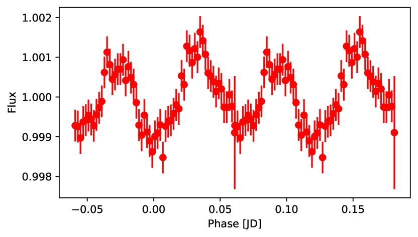
Figure 2: Example TESS light curve of an ellipsoidal system (PG1043+760) showing additionally Doppler beaming. The light curve is shown phase-folded to the orbital period and binned.

To look for reflection effect systems in the TESS light curves, we have searched TESS sectors 1-36 for variability in all stars brighter than $G<16\,\rm mag$ from the Gaia DR2 catalogue of hot subluminous stars (Geier et al., 2019), as well as the catalogue of spectroscopically confirmed hot subdwarf stars (in total 2883 targets with 2-min cadence light curves and 353 targets with 20-sec cadence light curves). (Geier, 2020).We have used the light curves made available by the TESS Science Processing Operations Center (SPOC) through the Barbara A. Mikulski Archive for Space Telescopes MAST, using the PDCSAP flux, which corrects the simple aperture photometry (SAP) by removing instrumental trends, as well as contributions to the aperture expected to come from neighbouring stars other than the target of interest given a pre-search data conditioning (PDC). This is essential for TESS, as the pixel size is almost $21\,\rm arc\,sec$. Through the CROWDSAP parameter, the pipeline also provides an estimate of how much of the flux in the aperture belongs to the target. To avoid possible zero-point inconsistencies between different sectors, we divided the flux by the mean flux in each sector for each star.

We used the Python package Astropy (Astropy Collaboration et al., 2013, 2018) to calculate the Lomb-Scargle periodogram (Lomb, 1976; Scargle, 1982) of all light curves up to the Nyquist frequency, oversampling by a factor of 10. Light curves were then phase-folded to the period corresponding to the strongest peak, or twice this period for ellipsoidal systems, which have first harmonic peaks stronger than the fundamental orbital frequency. Our custom script that downloads the light curves and generates diagnostic plots with the periodogram and phase-folded light curves is publicly available. We visually inspected the diagnostic plots for all targets to confirm any variability and selected all objects showing a reflection effect (with and without eclipses), as well as stars showing ellipsoidal deformation. All targets with confirmed light variations can be found in Table LABEL:refl.

Additionally, we inspected the TESS or K2 light curves of all hot subdwarfs with with orbits characterized by radial velocity measurements (Kupfer et al., 2015, and references in Table LABEL:tab). All light curves were downloaded, phase-folded to the orbital period, and binned using the Python package lightkurve (Lightkurve Collaboration et al., 2018). We computed the periodogram around the orbital period to search for any small peaks resulting from weak reflection or ellipsoidal deformation signals. For targets without any variations, we phase-folded the light curve to the orbital period derived by time-resolved spectroscopy and determined the signal-to-noise ratio. The results of our search are shown in Table 1, 5, and LABEL:tab. Example TESS light curves of a reflection effect system and an ellipsoidal system additional showing Doppler beaming can be found in Fig. 1 and 2. The complete set of light curves, along with full details regarding our modeling and analysis methods, will be presented in an additional paper (Paper II, Schaffenroth et al. in prep.).

3 Characterizing the primary star

3.1 Absolute magnitude and reduced proper motion

3.1.1 Method

Both hot subdwarf and hot WD binaries containing a cool, low-mass companions can show a reflection effect (Schaffenroth et al., 2019), as can some sdOs that are central stars of planetary nebula (CSPN). In order to determine the true nature of the primary star, we used the colors, parallaxes, and proper motion from Gaia EDR3 (Gaia Collaboration et al., 2021), as was done in Schaffenroth et al. (2019) for newly discovered HW Vir systems. Using the Gaia $G$ magnitude together with the parallax, we could determine the absolute magnitude of our targets using the distance modulus ($G-M_{G}=5\log_{10}d-5$). We ensured that all of our targets but one (which we identified as a potential triple system) had a small uncertainty in their parallax ($\lessapprox 10\%$) and a Renormalised Unit Weight Error (RUWE) below 1.4 (e.g., Penoyre et al., 2022). A higher RUWE indicates potential problems with the parallax.

Another way to confirm our target selection is to determine the reduced proper motions $H_{G}=G+5(\log\mu+1)$. Stars that are farther away should show less transverse velocity on average than those that are closer, and the reduced proper motion is therefore a proxy for the distance; closer objects should have larger reduced proper motions. Typically, hot subdwarfs show reduced proper motions between 5 and 14 mag (e.g. Schaffenroth et al., 2019).

3.1.2 Results

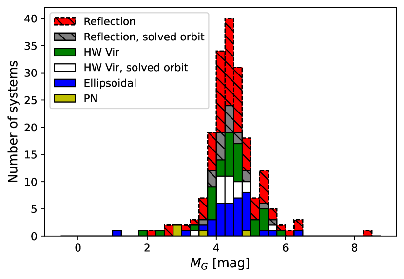
Figure 3: Gaia absolute magnitude $M_{G}$ of all our targets divided into different groups according to the different light curve variations they show as shown in the legend.

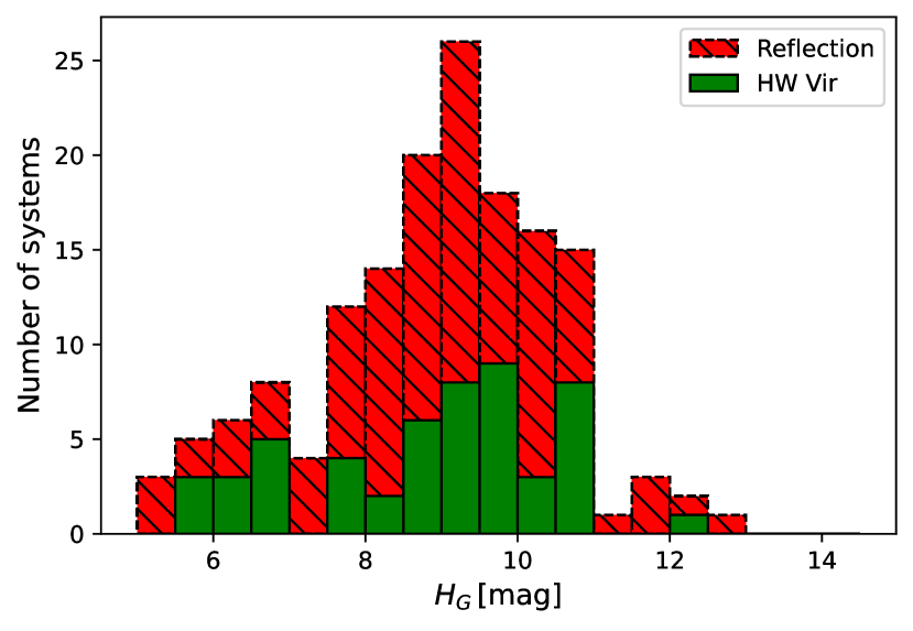
Figure 4: Reduced proper motion of all our reflection effect systems (eclipsing and non-eclipsing).

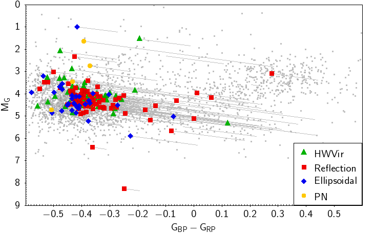
Figure 5: $G_{\rm BP}-G_{\rm RP}$ vs $M_{G}$ diagram. The targets are again grouped according to their light variations. All targets have been corrected for interstellar extinction using Stilism. The correction is shown with the grey lines. In comparison the known sdO/Bs taken from Geier (2020) are shown with the grey data points.

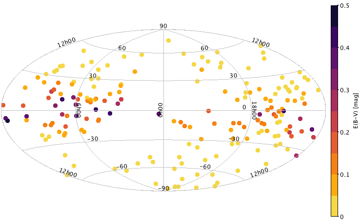
Figure 6: Position of our targets on the sky (in galactic coordinates). The color coding is giving by the color excess E(B-V).

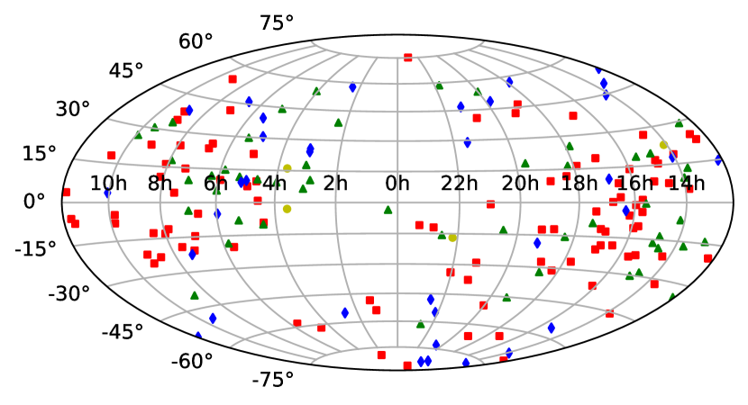
Figure 7: Comparison of the position of our targets on the sky (in galactic coordinates). The green triangles mark HW Virs, the red squares reflection effect systems and the blue diamonds ellipsoidal systems, and the yellow circles CSPNs.

The results are found in Table LABEL:refl. Inspecting the absolute magnitude $M_{G}$ distribution of all our targets (Fig. 3), we see that it peaks around $M_{G}=4.5$, as expected for hot subdwarf stars (Geier, 2020). We have only one target with $M_{G}>7\,\rm mag$, which is most likely a WD primary. We also have some targets with $M_{G}<3\,\rm mag$, which are known CSPN, or pre-ELM WD.

Our reduced proper motion distribution shown in Fig. 4 also confirms that our targets are most likely hot subdwarf stars.

Since hot subdwarfs are of spectral type O and B, they have temperatures between 25 000 to 50 000 K and blue colors. Their luminosities are lower than main sequence stars and higher than hot white dwarfs. To check where we find our targets in the color-magnitude diagram, we plot a $G_{\rm BP}-G_{\rm RP}$ vs $M_{G}$ diagram (see Fig. 5). Both the absolute magnitude and $G_{\rm BP}-G_{\rm RP}$ color were corrected for interstellar extinction using 3D maps (Lallement et al., 2014; Capitanio et al., 2017). Our targets are located at $-0.5<G_{\rm BP}-G_{\rm RP}<0.3$, with most of the targets clustering at $G_{\rm BP}-G_{\rm RP}<-0.25$. There is a slight trend that targets with $G_{\rm BP}-G_{\rm RP}>-0.25$ seem to have smaller $M_{G}$. As all of those targets show a high extinction, this trend can most likely be explained by insufficient correction of the interstellar extinction. The distribution of our targets on the sky (Fig. 6) shows that most of the targets with high extinction are found close to the galactic plane, up to $\pm 20^{\circ}$ away. The comparison with the known sdO/Bs from Geier (2020) shows quite a good agreement. One target is found with $G_{\rm BP}-G_{\rm RP}=0.3$ at an absolute magnitude $M_{G}=3$, consistent with known composite sdB stars. Only a few of our targets are found at $G_{\rm BP}-G_{\rm RP}<-0.45$, which is probably due to the fact that most of them are cooler helium-core burning sdB stars rather than evolved sdO stars. The comparison of the position of all our targets grouped together by the observed light variations (Fig. 7) shows that all different target types seem to be equally distributed on the sky.

3.2 Spectral energy distribution

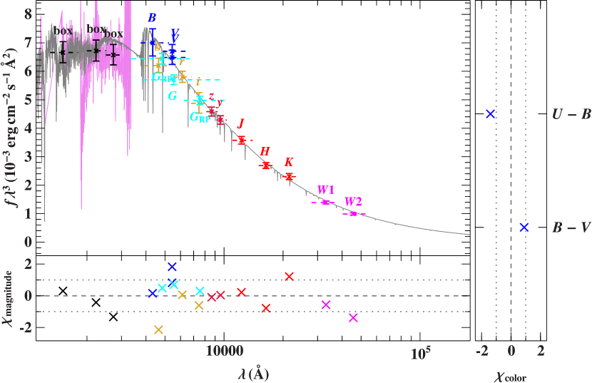
Figure 8: Example of an SED fit (for the sdB+WD system PG1519+640).

3.2.1 Method

To confirm a candidate’s status as a hot subdwarf, we need to derive the effective temperature $T_{\rm eff}$ and surface gravity $\log g$. The best way to determine atmospheric parameters is to observe and model the target’s spectrum. However, it is also possible to determine $T_{\rm eff}$, as well as the radius and the luminosity, by fitting the spectral energy distribution (SED) with synthetic spectra and combining this with the distance from the Gaia parallax (see Heber et al., 2018; Irrgang et al., 2021, for more details on this method). The shape of the SED gives us $T_{\rm eff}$ as well as the interstellar reddening. And by comparing the observed and synthetic flux $f(\lambda)$ and $F(\lambda)$ respectively, we can derive the angular diameter $\theta=0.5\sqrt{\frac{f(\lambda)}{F(\lambda)}}$, which can be used to derive the radius $R=\theta/(2\varpi)$ and the luminosity $L/L_{\odot}=(R/R_{\odot})^{2}(T_{\rm eff}/T_{\rm eff,\odot})^{4}$ by using the Gaia parallax $\varpi$ and parallax offset.

Using the $\log g$ determined by the spectral fitting and the radius determined by the SED and Gaia distance, we can also derive the mass of the hot subdwarf $M=gR^{2}/G$ for the hot subdwarf binaries with known atmospheric parameters.

3.2.2 Results

One example SED fit is shown in Fig. 8. Unfortunately, the SED fitting is not straightforward for the reflection effect systems since our targets show light variations and the photometry we used from the literature was taken at a random phase.

In light of the above, we tested our method on reflection effect and ellipsoidal systems with known atmospheric parameters and sufficient photometric data (see Table LABEL:sed_known for the results). The comparison between effective temperatures determined by spectral fitting and spectral energy distribution fitting (Fig. 9) shows that for systems with $T_{\rm eff}\lessapprox 32\,000\rm\,K$, the fitting of the SED can determine the $T_{\rm eff}$ very well if we neglect infrared photometry, since the contribution of the companion gets larger there. UV (IUE or Galex FUV or NUV) and SDSS u’ photometry are essential for disentangling the effect of $T_{\rm eff}$ and interstellar reddening on the SED by covering the Balmer jump, so we exclude all targets without sufficient UV photometry from the SED fitting. For hotter systems, we see a larger scatter. For $T_{\rm eff}>42\,000\,\rm K$ the Balmer jump is not visible anymore, and so the temperature cannot be derived anymore without constraining the interstellar reddening. There is also a slight tendency that the SED fitting derives smaller temperatures than the spectral fitting.

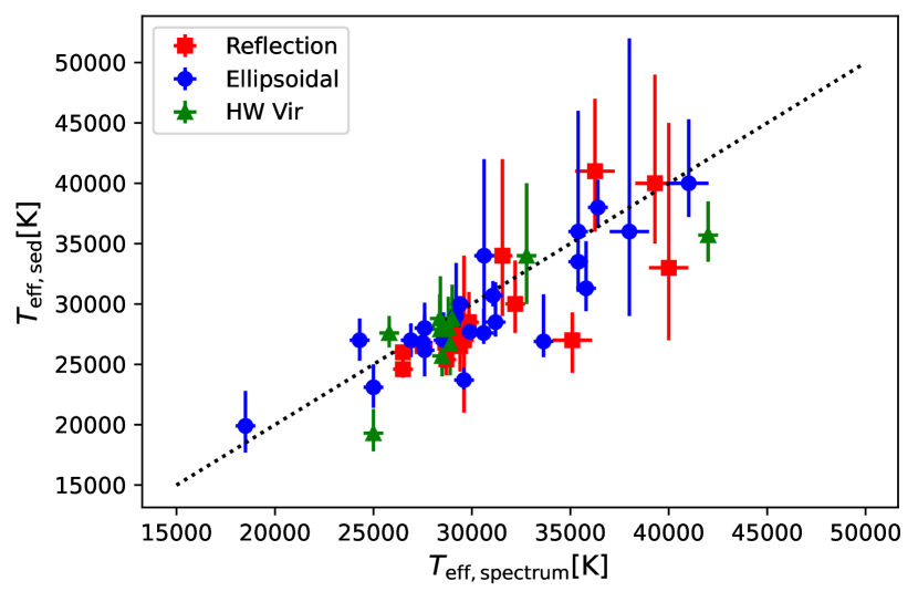
Figure 9: Comparison of the effective temperature determined by spectral fitting and spectral energy distribution fitting. Blue circles mark systems showing ellipsoidal deformation, green triangles mark HW Vir systems and red squares mark reflection effect systems.

Using the derived luminosities, we construct a Hertzsprung-Russell diagram for reflection effect and ellipsoidal systems with spectroscopic parameters for the first time. This is shown in Fig. 10. The sdBs on the EHB with temperatures below 33000 K are found at similar luminosities between 15 and 40 $\rm L_{\odot}$. At larger temperatures the luminosity increases with the temperature but also a larger scatter is visible resulting from larger differences in the radii. Németh et al. (2012) showed that the He abundances and the difference in He abundance increases with the temperature. The larger scatter of the radii and hence the luminosity at larger temperatures may be related to those He abundance differences.

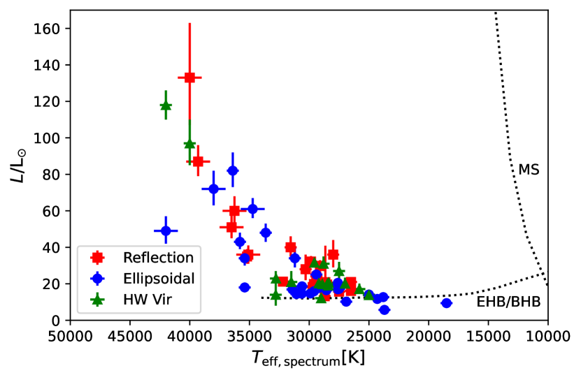
Figure 10: Hertzsprung-Russell diagram of our targets with known atmospheric parameters. Blue circles mark systems showing ellipsoidal deformation, green triangles mark HW Vir systems and red squares mark reflection effect systems. The dotted lines mark the zero-age main sequence or EHB/BHB.

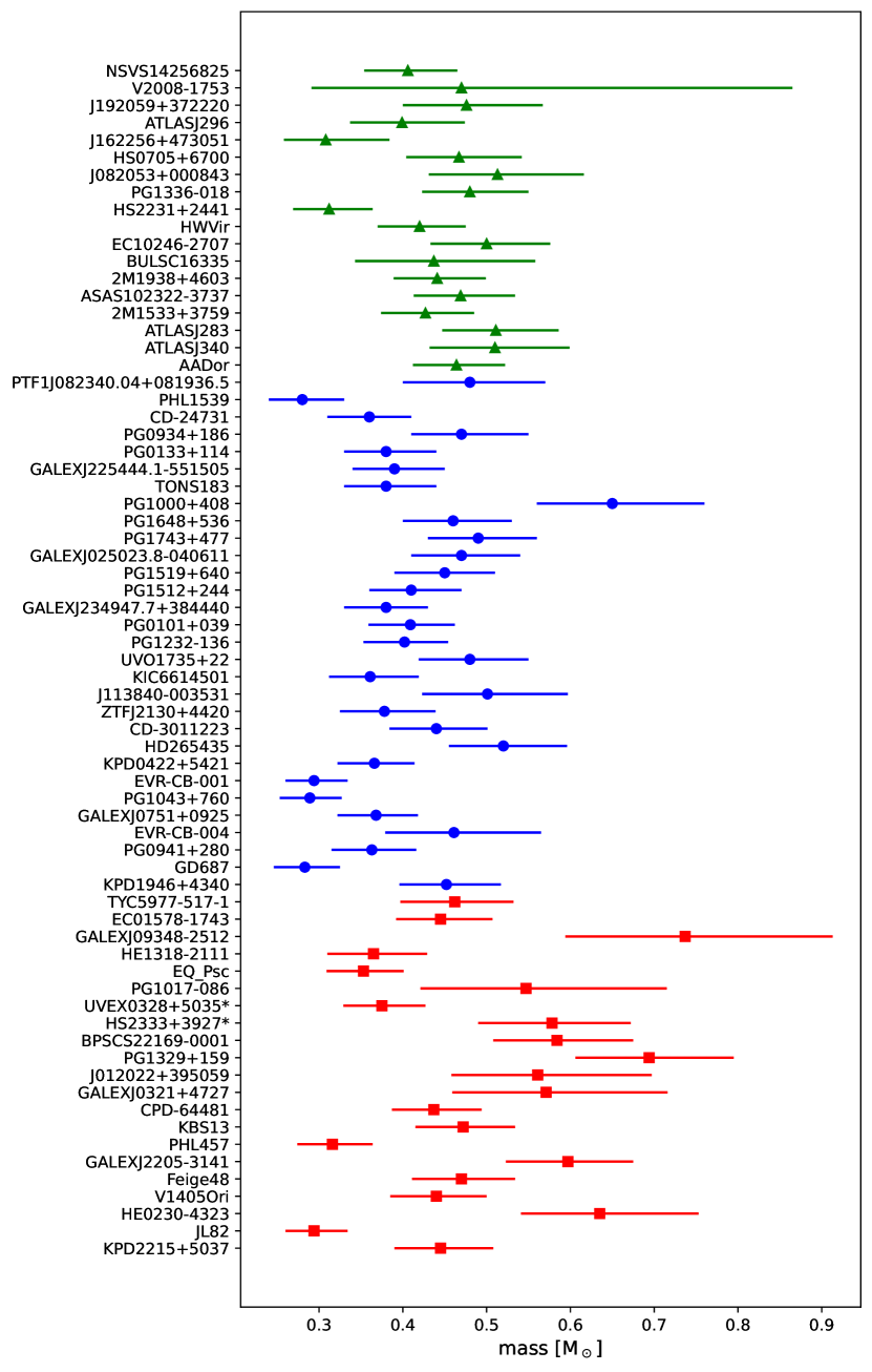
Figure 11: Masses determined by combining the spectroscopic analysis with the fit of the SED and the Gaia parallaxes. Blue symbols mark systems showing ellipsoidal deformation, green symbols mark HW Vir systems and red symbols mark reflection effect systems.

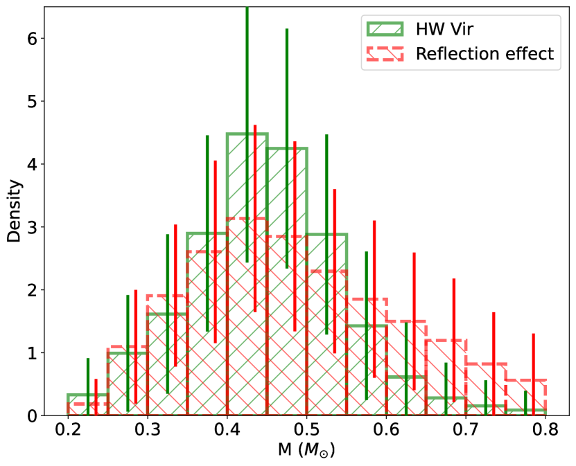
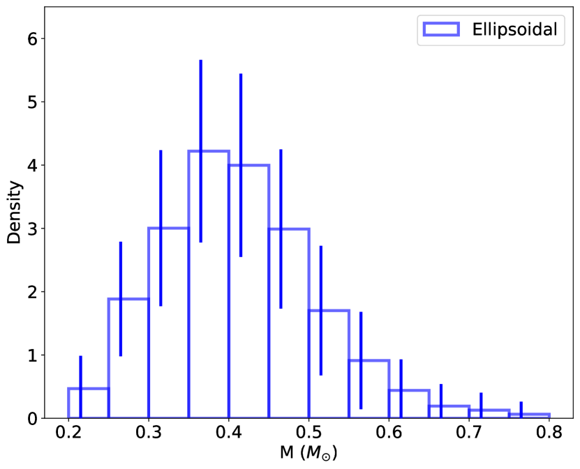
Figure 12: Histogram of the masses determined by combining the spectroscopic analysis with the fit of the SED and the Gaia parallaxes.

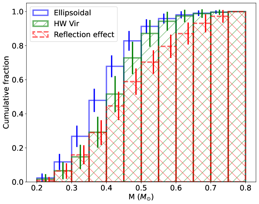
Figure 13: Cumulative distribution of the masses determined by combining the spectroscopic analysis with the fit of the SED and the Gaia parallaxes.

With the spectroscopic $\log{g}$ and the radius from the SED fitting, we were able to derive the mass distribution of reflection effect, HW Vir and ellipsoidal systems. A similar approach was used in Krzesinski & Balona 2022, which derived the mass distribution of pulsating hot subdwarf candidates with spectroscopic parameters to be a broad peak with the maximum at $0.45\,\rm M_{\odot}$. However, they state that their analysis might not be reliable and useful to derive masses of single systems.

Our result is shown in Fig. 11, 12 and 13 and Table LABEL:sed_known. For the HW Vir systems, we derive a mass of $0.46^{+0.08}_{-0.12}\,\rm M_{\odot}$ using a skewed normal distribution. As the typical mass error is about 0.05 $\rm M_{\odot}$ this suggests an intrinsically broader peak. The non-eclipsing reflection effect systems seem to have a broader peak with more higher-mass sdBs. As the only difference compared to the HW Vir systems is that they have no eclipses, we would not expect any difference. Determining atmospheric parameters from reflection effect systems has to be done with caution, as the contribution of the companion to the total flux changes with the orbital phase causing the reflection effect. So the atmospheric parameters have to be determined at or close to phase zero, when only the cool side of the companion is visible, or at the secondary eclipse, when the companion is occulted by the sdB in an eclipsing system. Most of the atmospheric parameters of the reflection effect systems have been determined from a single spectrum or co-added spectra at different orbital phases, causing systematic shifts to higher temperatures and higher $\log{g}$. This influences the determination of the radius and will result in a shifted mass. The HW Vir systems have been studied much more carefully, and so their determined atmospheric parameters are much more reliable.

The masses of the sdBs with white dwarf companions show a distribution with a similar width but a peak shifted to lower masses at $0.38^{+0.12}_{-0.08}\,\rm M_{\odot}$. The distribution also seems to be slightly asymmetric, extending to higher masses. The cumulative distribution shows the shift in mass more clearly, and shows that it is indeed significant.

The samples were taken from the literature and are not complete but are suffering from selection effects, which are not easy to determine. However, in the Gaia color-magnitude diagram (Figure. 5) and the sky distribution (Fig. 7), we can see that sdB+WD and the sdB+dM populations are overlapping well. The sdBs in the systems of both populations have been identified the same way by color selection. Hence, we expect that the selection effects should be similar for both populations and that they are comparable nevertheless.

The sdB+WD systems have been found preferably by RV variations in contrast to the HW Vir systems, as the sdB+WD systems show much smaller light variations. Both samples included only systems at the short period end of their period distribution (see Table LABEL:refl). A larger sample over a larger period range for both populations will be necessary to confirm our findings and also find or exclude differences of the sdB mass in systems with different orbital periods.

By fitting the SED and combining this with the Gaia parallax we can also constrain the atmospheric parameters of our reflection effect candidates, which do not have spectroscopic parameters, by fiting the SED and assuming a canonical mass for the sdB. From the radius we derive, we can constrain the $\log g$ in this way and constrain the atmospheric parameters for 44 targets with sufficient UV photometry. The results can be found in Table 4. The atmospheric parameters are compared to the solved systems in the $T_{\rm eff}-\log{g}$ diagram (Fig. 14). This shows that our reflection effect candidate systems are mostly found on the EHB. Some of the candidates are on post-EHB tracks, which means the He in the core was exhausted and they are evolving away from the EHB. Only one candidate was found above the EHB, which could be a lower mass pre-He WD.

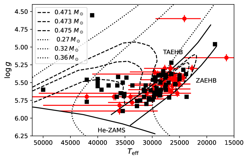
Figure 14: $T_{\rm eff}-\log{g}$ diagram of the sdB binaries with spectroscopic parameters (black squares) compared to the reflection effect candidates (red diamonds). The black solid lines mark the zero-age extreme horizontal branch (ZAEHB), the terminal-age extreme horizontal branch (TAEHB) and the He-main sequence (He ZAMS). The dashed lines are evolutionary tracks by Dorman et al. (1993) for sdB masses of 0.471, 0.473, and 0.475 $\rm M_{\odot}$. The dotted lines are tracks for extremely low mass white dwarfs of a mass of 0.27, 0.32, and 0.36 $\rm M_{\odot}$ by Althaus et al. (2013).

4 The period distribution from light variations found by TESS

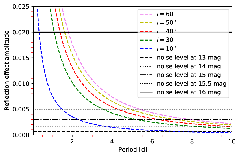
Figure 15: Amplitude of the reflection effect of a typical sdB+dM system for different periods and inclinations. The black lines mark the TESS noise level for stars of different brightness.

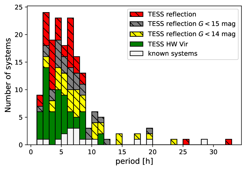
Figure 16: Period distribution of the reflection effect systems with and without eclipses observed by TESS. The known reflection effect systems are marked in white, the eclipsing reflection effect systems are marked in red, and the reflection effect systems without eclipses are marked in yellow, green and grey for systems with $G<13\,\rm mag,G<14\,mag$ and all other systems respectively.

4.1 The selection effects of TESS

In order to judge the completeness of our reflection effect sample, we simulated the expected amplitude of the reflection effect for a typical sdB+dM system with different orbital periods and compared this to the noise level of the TESS satellite for stars of different brightness (see Fig. 15). This was done by checking the noise level in the light curves of different sdB stars of the same brightness not showing any variations in the light curve. For a 15 mag system, the detection limit is about 0.3%. As expected, the amplitude of the variations decreases with lower inclination. But even with a low inclination of only $10^{\circ}$, we would expect to detect the reflection effect for a system brighter than 15 mag with TESS up to two days, for higher inclinations of about $40^{\circ}$ up to about 6 days, and in inclinations of more than $60^{\circ}$ up to 8 days. Since the reflection effect becomes more sinusoidal at low inclinations, it is quite hard to distinguish it from other variations like pulsations or spots. Consequently, we will probably find low-inclination reflection effects only for the systems in which the period is already known from the RV curve. But the inclination should correlate with the period, and so this should not influence the period distribution we derive.

Another selection effect could come from TESS having such large pixels (21 arc-sec per pixel). If another star of comparable or higher brightness is close to the star, the light curve can become contaminated. TESS tries to correct for this additional flux through its reported PDCSAP flux, and it uses the CROWDSAP keyword in the header to quantify the contamination level. This correction can over- or underestimate the flux, and so the amplitude is not entirely reliable when a bright star is so close and it contributes significantly to the flux in the target pixel. This means that we might miss some reflection effect systems when unrelated stars are too close, but overall this correction seems to be quite good (a few percent difference; see Paper II for more details) and there is no reason why this should influence the period distribution of the detected systems.

As the amplitude of the ellipsoidal modulation is much smaller as can seen in Fig. 2, this is very different for sdB+WD systems because we will only find the systems with the closest periods and/or highest mass companions by our light variation search, if the period is not known by RV variations for example.

4.2 Period distribution of the reflection effect systems

Taking all of this into account, we will never acquire a complete sample of reflection effect binaries from light curves alone, and the situation is even worse for the ellipsoidal systems. We do expect to find most reflection systems with higher inclinations observed by TESS up to periods around 7 days, as they can be identified from their light curve shapes with ease. Fig. 16 presents our observed orbital period distribution for sdBs with cool, low-mass companions. To ensure we do not see any difference with the brightness, we also checked the distributions of reflection effect systems of different brightness with a two-sample Kolmogorov–Smirnov test, but we could not find any significant differences. The period distribution shows that the reflection effect systems without eclipses tend to be found at periods longer than the eclipsing systems. This is expected as the eclipse probability decreases quickly with increasing separation distance and period. The period distribution shows a broad peak from 2-8 hours and falls off quickly on either end. There are very few systems with periods shorter than 2 hours, and none are below 1.2 hours. Above 8 hours, the distribution falls off quickly, and only a handful of systems are found beyond 20 hours. Despite our ability to detect systems with periods up to several days, the longest–period system we have found has a period of 35 hours. Since we do not find any longer–period systems, they either do not exist, or they are incredibly rare. As TESS continues to observe more and more reflection effect systems and increase the sample size, hopefully this question can be answered.

5 The companions of the close sdB binaries with solved radial velocity curves

5.1 The nature of the companion

As we have seen, the reflection effect generates a flux variation that is detectable at periods up to several days. The light variation from ellipsoidal deformation or Doppler beaming, however, is much weaker on average (below 0.1-0.2%) at periods up to about one day and not detectable at longer periods. We can use these facts to differentiate between cool, low-mass companions and white dwarf companions (more details and the analysis of those systems is shown in Paper II) for the systems with periods known from RV variations.

We phased the available light curves of all hot subdwarfs with solved orbits (135 of the 165 systems have Kepler or TESS light curves). Of those, 40 show a reflection effect and 33 show ellipsoidal deformation or Doppler beaming indicating that they have a white dwarf companion (see Paper II for more details). The rest do not show significant variations at the orbital period. We derived the signal-to-noise ratio for all light curves not exhibiting any variations. The result can be found in Table 5.

To constrain the nature of the companion, we used the amplitude estimates at a given period and inclination shown in Fig. 15. Under the assumption all orbital plane orientations are equally probable, the probability of the inclination being lower than $10^{\circ}$ is only $1-\cos 10^{\circ}=1.5\%$ (Gray, 2005). Therefore, we classify as sdB+WD systems all sdB binaries with light curves having a signal-to-noise ratio smaller than the amplitude expected for a reflection effect system observed at an inclination angle $<10^{\circ}$ (probability $>98.5\%$).

Moreover, for companion masses larger than 0.45 $\rm M_{\odot}$ we would expect to see an infrared excess in the SED, if the companion would be a main sequence companion. Therefore, we also classify all sdB binaries with minimum companion masses $>0.45\,\rm M_{\odot}$ as sdB+WD system. The minimum companion masses can be derived by the mass function

$$f(M_{1},M_{2})=\frac{M_{2}^{3}\sin^{3}i}{(M_{1}+M_{2})^{2}}=\frac{PK_{1}^{3}}{2\pi G},$$ (1)

assuming a mass of 0.47 $\rm M_{\odot}$ for the sdB and an inclination of 90^∘. We are unable to constrain the nature of the companion in this way for only 12 of our systems, as the noise in their light curves is too large and the minimum companion mass is too small. In total, this gives us 83 sdB+WD systems and allows us to constrain the nature of 75% of all close sdB binaries with solved orbits.

Most of the sdB binaries with solved orbits have been detected by radial velocity variations, a method biased towards shorter periods, higher companion masses, and higher inclinations. Only very few of these were found by light variations. In this sample, about one-third of the sdB binaries have M dwarf or brown dwarf companions, and two-thirds have white dwarf companions.

5.2 The period distributions

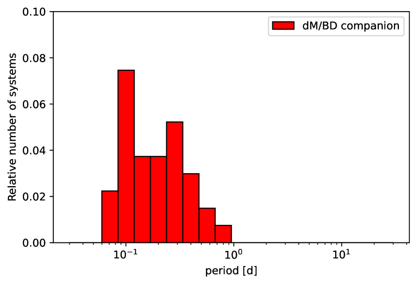
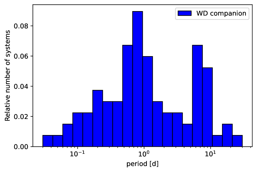
Figure 17: Period distribution of the hot subdwarf binaries with solved orbits with dM/BD companions in the top panel, with WD companions in the middle and unknown companions in the lower panel.

The updated period distributions of the dM/BD and WD companions and their differences are also interesting, as shown in Fig. 17. We already discussed the distribution of the reflection effect and HW Vir systems showing periods from 2 hours to about 1 day. The systems with WD companions, on the other hand, show a broad distribution from just about one hour to 27 d. On top of this broad distribution we find two distinct peaks at around one day and around 5-10 days. The companion is still undefined only for a small number of systems. Most of them have periods longer than one day, agreeing well with the distribution of the WD companions, so it is likely they are also sdB+WD systems.

5.3 The minimum companion masses

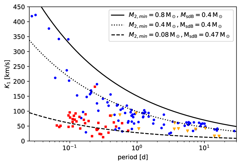
Figure 18: RV semi-amplitudes of all known short-period sdB binaries with spectroscopic solutions and with TESS or Kepler light curves plotted against their orbital periods (red squares: dM/BD companions, blue circles: WD companions, yellow diamonds: unknown type). The lines mark a certain minimum companion mass derived from the binary mass function (assuming 0.47 or 0.4 $\,M_{\odot}$ for the sdBs).

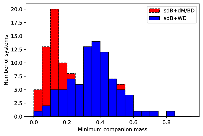
Figure 19: Minimum companion mass distribution of all known short-period sdB binaries with spectroscopic solutions and with TESS or K2 light curves (assuming 0.47 $\,M_{\odot}$ for a sdB with dM/BD companion or 0.4 $\,M_{\odot}$ for a sdB with WD companion).

To get a clearer picture of the masses of the close companions to hot subdwarf stars, we update the plot of RV semi-amplitude versus orbital period for all known sdB binaries (as shown in Kupfer et al. 2015) with spectroscopic solutions and with TESS or Kepler light curves (Fig. 18) as well as plot the minimum companion mass distribution in Fig. 19.

Our new sample adds many more systems with companion mass constraints to this plot. As we have seen, it is possible to constrain the minimum mass of the companion from the RV semi-amplitude of the sdB and the orbital period, when assuming a mass for the sdB. This is given by the black lines for different periods. For a random distribution of system angles, the probability to have a system with inclination $>60^{\circ}$ is the same as for an inclination of $<60^{\circ}$, and so about half of the companions should have masses of only up to 20% higher than the minimum companion mass.

We find that systems with cool, low-mass companions cluster around the hydrogen-burning limit with masses up to $0.25\,\rm M_{\odot}$ with one exception. The white dwarf companions to sdB stars have higher minimum masses, and it looks like there are three different populations. At the shortest periods from approximately one to about three hours, a small group of WD companions with minimum companion masses around 0.7 to 0.8 $\rm M_{\odot}$ are found. Most of the WD companions are found in binaries with longer periods. Up to a period of about 4 days they seem to have significantly lower minimum companion masses with a mass ratio close to one (around $0.4\,\rm M_{\odot}$, when assuming an sdB mass of $0.4\,\rm M_{\odot}$). Systems with periods belonging to the second peak in the period distribution around 5-10 days show some indication of slightly higher minimum companion masses above $0.4\,\rm M_{\odot}$ up to $0.6\,\rm M_{\odot}$.

6 Discussion and Conclusions

Our light variation search increases the number of known reflection effect systems from 19 to 104 systems. Moreover, we detected 23 new sdB+WD systems showing tiny variations with amplitudes below $\sim 0.1\%$, due to Doppler beaming or ellipsoidal deformation in their light curves.

The characterization of the reflection effect systems in our sample shows that all except one have hot subdwarf primaries. The one exception was a system with a white dwarf primary. Similar results were found in other surveys, such as EREBOS (Schaffenroth et al., 2019). The detection of a white dwarf primary is not a complete surprise since we selected targets from the Gaia DR2 catalogue of hot subluminous stars, which does have some overlap with the white dwarf catalogue. Nonetheless, most of the primaries in our systems should be sdO/B stars. The reflection effect is only visible in hot white dwarfs, which are much rarer. Moreover, white dwarfs are much fainter than hot subdwarf stars. And since sdBs are mainly formed by binary evolution, the binarity rate of sdBs is much higher than of WDs. That is why reflection effect systems with hot subdwarf primaries will dominate all surveys for reflection effect systems.

To check the mass determination of the sdB using the SED and the Gaia parallaxes, we compared the masses derived by this method with the masses derived by the light curve analysis of several ellipsoidal systems. This is shown in Table 2. The masses derived by the two different methods agree very well within the errors for all systems, thereby showing the validity of our spectrophotometric Gaia distance method.

The comparison of the mass distribution of the sdB+dM and the sdB+WD (Fig. 12) shows that they differ significantly. The mass distribution of sdBs with WD companions is shifted to lower masses compared to sdBs with dM/BD companions. This implies that sdBs with dM/BD companions come from a different population than sdBs with WD companions. The sdB+dM systems show a peak around the canonical mass for He burning and a few systems at higher and lower mass, as predicted by binary population synthesis models (Han et al., 2002, 2003). Those non-canonical systems can originate from young, higher-mass systems igniting He in the core under non-degenerate conditions or be pre-He WDs not massive enough for He-burning that are passing through the sdB region in the HRD. The sdB+WDs, on the other hand, show many more low-mass systems. The sdB binaries with massive companions are observed towards the Galactic plane, where younger stars are found. This indicates that those systems are preferably formed in younger populations than the sdB+dM stars. The other sdB+WD systems seem to be equally distributed on the sky (see Fig. 7).

Table 2: Masses of the solved sdB+WD systems derived by light curve analysis and SED fitting

target	$M_{\rm sdB,SED}$	$M_{\rm sdB,lc}$	references
	[$\rm M_{\odot}$]	[$\rm M_{\odot}$]
KPD1946+4340	$0.452^{+0.065}_{-0.056}$	$0.47^{+0.03}_{-0.03}$	Bloemen et al. (2011)
CD-3011223	$0.44^{+0.061}_{-0.056}$	$0.47^{+0.03}_{-0.03}$	Geier et al. (2013)
PTF1J0823+0819	$0.48^{+0.09}_{-0.08}$	$0.45^{+0.09}_{-0.07}$	Kupfer et al. (2017b)
EVR-CB-001	$0.294^{+0.04}_{-0.034}$	$0.21^{+0.05}_{-0.05}$	Ratzloff et al. (2019)
EVR-CB-004	$0.461^{+0.104}_{-0.082}$	$0.52^{+0.04}_{-0.04}$	Ratzloff et al. (2020b)
ZTFJ2130+4420	$0.378^{+0.061}_{-0.053}$	$0.337^{+0.015}_{-0.015}$	Kupfer et al. (2020b)
HD265435	$0.59^{+0.17}_{-0.14}$	$0.64^{+0.10}_{-0.09}$	Pelisoli et al. (2021)

The observation of space-based, high S/N light curves covering a time span of at least 27 days up to several months of so many sdBs gave us for the first time a large sample of reflection effect binaries. Since they were selected mainly from the Gaia hot subdwarf catalogue and had no prior RV measurements, this gives us the first period distribution of sdB+dM systems selected only by light variations. The orbital period distribution of post-CE binaries is mainly dependent on the criterion for the ejection of the CE (Han et al., 2002), and so this distribution can be used to constrain the common-envelope phase when combined with the companion mass distribution as done in Ge et al. (2022) for the sample of hot subdwarf binaries from Kupfer et al. (2015) or comparing it to a modelled sdB binary sample using binary population synthesis.

Aided by high-quality TESS light curves, we could constrain the nature of the companion in 75% of the sdB binaries with solved orbits and compare them. As seen in Fig. 17, the period distribution of the sdB+dM systems is concentrated in a much smaller period range compared to the sdB+WD systems, which are found over a wide range of periods from 0.03-30 days. The distribution of the minimum companion masses found at a certain orbital period (Fig. 18) shows that the companions in the reflection effect systems have minimum masses typical for BD/dM systems ($0.05-0.2\,\rm M_{\odot}$). There is no change with the orbital period visible. For the sdB+WD systems this is different. There seem to be two distinct groups of companion masses. At the shortest periods below 0.1 d, WD companions with high minimum masses around $0.8\,\rm M_{\odot}$ are found, which could be CO or ONe WDs. At longer periods, the WD companions seem to have significantly lower minimum masses, with masses around $0.4\,\rm M_{\odot}$. Many of those could be He-WD companions. At the longest periods the masses seem to be slightly higher indicating a third population of low-mass CO WD companions. This could suggest that sdB+WD systems at the shortest periods come from a different population with higher-mass progenitors having higher-mass companions than the longer period sdB+WD systems, which is consistent with predictions by binary population synthesis (Han et al., 2002, 2003).

The high signal-to-noise light curves allowed us to derive parameters for a large number of sdB+dM/BD and sdB+WD systems. Details of this light curve modeling and analysis are discussed in a separate paper (Paper II).

As TESS continues to observe, the number of high-quality reflection effect and sdB+WD light curves will continue to grow. This will further increase our sample size and improve constraints on the mass and period distributions. Future spectroscopic and photometric surveys like 4MOST, BlackgGem, and Vera Rubin Observatory will also increase our sample size and our knowledge about these systems.

Appendix A Parameters of the close sdB binaries in TESS

Table 3: Atmospheric and absolute parameters of the sdB binaries with spectroscopic parameters and with space-based light curves determined by spectroscopy and spectral energy distribution fitting together with the Gaia parallax.

target	$T_{\rm eff,spec}$	$\log{g}_{\rm spec}$	$T_{\rm eff,sed}$	$M_{\rm sed}$	$L_{\rm sed}$	$R_{\rm sed}$
	[K ]	[cgs]	[K]	[M⊙]	[L⊙]	[R⊙]
Reflection effect systems
KPD2215+5037	29600 $\pm$ 1000	5.64$\pm$ 0.10	$27000^{+7000}_{-6000}$	$0.445^{+0.063}_{-0.055}$	$19.9^{+1.9}_{-1.7}$	$0.170^{+0.005}_{-0.005}$
JL82	26500$\pm$ 500	5.22$\pm$ 0.1	$26000^{+500}_{-600}$	$0.294^{+0.04}_{-0.034}$	$21^{+1.9}_{-2.0}$	$0.222^{+0.006}_{-0.006}$
HE0230-4323	31552$\pm$ 500	5.60$\pm$ 0.07	$34000^{+8000}_{-5000}$	$0.635^{+0.118}_{-0.094}$	$40^{+6}_{-5}$	$0.211^{+0.014}_{-0.012}$
V1405Ori	35100$\pm$ 800	5.66$\pm$ 0.11	$27000^{+2300}_{-2700}$	$0.44^{+0.06}_{-0.055}$	$36^{+5}_{-5}$	$0.166^{+0.006}_{-0.006}$
Feige48	29850$\pm$500	5.46$\pm$0.05	$28500^{+2500}_{-1800}$	$0.47^{+0.064}_{-0.059}$	$32.2^{+3}_{-2.8}$	$0.213^{+0.007}_{-0.007}$
GALEXJ2205-3141	28150$\pm$500	5.68$\pm$0.10	$26800^{+1100}_{-1000}$	$0.597^{+0.078}_{-0.074}$	$20.9^{+20}_{-1.8}$	$0.186^{+0.005}_{-0.005}$
PHL457	26500$\pm$1100	5.38$\pm$0.12	$24600^{+1200}_{-700}$	$0.316^{+0.048}_{-0.042}$	$16.1^{+1.9}_{-1.8}$	$0.191^{+0.008}_{-0.008}$
KBS13	29700$\pm$500	5.70$\pm$0.05 -	$0.472^{+0.062}_{-0.057}$	$18.2^{+1.6}_{-1.5}$	$0.162^{+0.004}_{-0.004}$
CPD-64481	27500$\pm$500	5.60$\pm$0.05	$26500^{+1200}_{-500}$	$0.437^{+0.057}_{-0.050}$	$15.7^{+1.3}_{-1.3}$	$0.1748^{+0.0032}_{-0.0030}$
GALEXJ0321+4727	27990$\pm$400	5.34$\pm$0.07	-	$0.571^{+0.145}_{-0.112}$	$36^{+8}_{-7}$	$0.219^{+0.005}_{-0.004}$
J012022+395059	29400$\pm$500	5.48 $\pm$0.05	$26500^{+2100}_{-2100}$	$0.561^{+0.136}_{-0.103}$	$24^{+6}_{-4}$	$0.194^{+0.019}_{-0.016}$
PG1329+159	29100$\pm$900	5.62$\pm$0.10	$27400^{+1100}_{-1000}$	$0.694^{+0.101}_{-0.088}$	$29.8^{+3.1}_{-2.9}$	$0.215^{+0.008}_{-0.008}$
BPSCS22169-0001	39300$\pm$500	5.600$\pm$0.05	$40000^{+9000}_{-5000}$	$0.584^{+0.091}_{-0.076}$	$87^{+9}_{-8}$	$0.202^{+0.009}_{-0.008}$
HS2333+3927	36500$\pm$1000	5.70$\pm$0.10	-	$0.578^{+0.094}_{-0.088}$	$51^{+7}_{-6}$	$0.177^{+0.011}_{-0.010}$
UVEX0328+5035	28500$\pm$(500)	5.500$\pm$(0.05)	-	$0.375^{+0.052}_{-0.046}$	$19.6^{+1.9}_{-1.8}$	$0.182^{+0.006}_{-0.006}$
PG1017-086	30300$\pm$500	5.61$\pm$0.10	-	$0.547^{+0.168}_{-0.126}$	$28^{+8}_{-6}$	$0.196^{+0.025}_{-0.021}$
EQ Psc	28700$\pm$500	5.63$\pm$0.05	$25400^{+1300}_{-1300}$	$0.353^{+0.048}_{-0.044}$	$13.2^{+1.3}_{-1.2}$	$0.151^{+0.005}_{-0.005}$
HE1318-2111	36300$\pm$1000	5.42$\pm$ 0.1	$41000^{+6000}_{-5000}$	$0.365^{+0.064}_{-0.055}$	$60^{+8}_{-8}$	$0.196^{+0.012}_{-0.011}$
GALEXJ09348-2512a	40800$\pm$500	5.55$\pm$0.05	$33000^{+12000}_{-6000}$	$0.737^{+0.176}_{-0.143}$	$133^{+30}_{-26}$	$0.241^{+0.023}_{-0.020}$
EC01578-1743a	32200$\pm$500	5.75$\pm$0.05	$30000^{+3600}_{-2400}$	$0.445^{+0.062}_{-0.053}$	$21.2^{+1.9}_{-1.7}$	$0.148^{+0.005}_{-0.004}$
TYC5977-517-1a	35200$\pm$500	5.69$\pm$0.05	$-$	$0.462^{+0.07}_{-0.065}$	$35^{+4}_{-4}$	$0.162^{+0.08}_{-0.007}$
HW Vir systems
AADor	42000$\pm$1000	5.460$\pm$0.05	$35700^{+2800}_{-2200}$	$0.464^{+0.058}_{-0.052}$	$118^{+8}_{-8}$	$0.206^{+0.005}_{-0.005}$
ATLASJ340	40000$\pm$1000	5.450$\pm$0.05	-	$0.510^{+0.098}_{-0.078}$	$116^{+16}_{-14}$	$0.225^{+0.014}_{-0.013}$
ATLASJ283	50000$\pm$ 1000	5.600$\pm$0.05	-	$0.511^{+0.075}_{-0.064}$	$201^{+17}_{-16}$	$0.189^{+0.008}_{-0.007}$
2M1533+3759	29200$\pm$500	5.58$\pm$0.05	-	$0.427^{+0.058}_{-0.053}$	$20.3^{+2.0}_{-1.8}$	$0.176^{+0.006}_{-0.005}$
ASAS102322-3737	28400$\pm$500	5.600$\pm$0.05	$27900^{+4400}_{-2800}$	$0.469^{+0.065}_{-0.056}$	$19.1^{+1.9}_{-1.6}$	$0.181^{+0.006}_{-0.005}$
2M1938+4603	29600$\pm$500	5.43$\pm$0.05	-	$0.441^{+0.058}_{-0.052}$	$31.6^{+2.7}_{-2.5}$	$0.213^{+0.006}_{-0.005}$
BULSC16335	31500$\pm$500	5.70$\pm$0.05	-	$0.437^{+0.121}_{-0.094}$	$21^{+6}_{-5}$	$0.156^{+0.018}_{-0.016}$
EC10246-2707	28900$\pm$500	5.64$\pm$0.05	$26700^{+2900}_{-2600}$	$0.500^{+0.076}_{-0.067}$	$19.8^{+2.3}_{-2.0}$	$0.178^{+0.008}_{-0.007}$
HWVir	28500$\pm$500	5.63$\pm$0.05	$25700^{+1900}_{-1700}$	$0.42^{+0.055}_{-0.050}$	$19.9^{+1.9}_{-1.7}$	$0.190^{+0.005}_{-0.005}$
HS2231+2441	28400$\pm$500	5.39$\pm$0.05	$28800^{+2000}_{-1500}$	$0.312^{+0.052}_{-0.043}$	$20.6^{+2.6}_{-2.3}$	$0.189^{+0.010}_{-0.009}$
PG1336-018	32800$\pm$500	5.76$\pm$0.05	$34000^{+6000}_{-4000}$	$0.480^{+0.070}_{-0.057}$	$22.9^{+2.3}_{-2.0}$	$0.153^{+0.005}_{-0.005}$
J082053+000843	25800$\pm$300	5.52$\pm 0.04$	$27600^{+1400}_{-1200}$	$0.513^{+0.103}_{-0.082}$	$17.1^{+3.0}_{-2.5}$	$0.208^{+0.017}_{-0.015}$
HS0705+6700	28800$\pm$900	5.40$\pm$0.10	$28000^{+2600}_{-2200}$	$0.467^{+0.075}_{-0.063}$	$31^{+4}_{-4}$	$0.225^{+0.011}_{-0.010}$
J162256+473051	29000$\pm$600	5.65$\pm$0.06	$28800^{+2800}_{-2000}$	$0.308^{+0.076}_{-0.05}$	$12.1^{+2.7}_{-2.0}$	$0.139^{+0.014}_{-0.011}$
ATLASJ296	25000$\pm$500	5.45$\pm$0.05	$19300^{+2000}_{-1500}$	$0.399^{+0.075}_{-0.062}$	$13.8^{+2.2}_{-1.9}$	$0.199^{+0.013}_{-0.012}$
J192059+372220	27500$\pm$1000	5.40$\pm$0.10	-	$0.476^{+0.091}_{-0.076}$	$27^{+5}_{-4}$	$0.230^{+0.016}_{-0.014}$
V2008-1753	32800$\pm$250	5.83$\pm$0.04	-	$0.47^{+0.395}_{-0.179}$	$14^{+13}_{-6}$	$0.124^{+0.042}_{-0.026}$
NSVS14256825	40000$\pm$500	5.50$\pm$0.05 5	-	$0.406^{+0.059}_{-0.052}$	$82^{+7}_{-8}$	$0.189^{+0.007}_{-0.007}$
Ellipsoidal and beaming systems
KPD1946+4340	34200$\pm$500	5.43$\pm$0.10	-	$0.452^{+0.065}_{-0.056}$	$61^{+6}_{-5}$	$0.216^{+0.008}_{-0.007}$
GD687	24300$\pm$500	5.32$\pm$0.07	$27000^{+1800}_{-1700}$	$0.283^{+0.042}_{-0.037}$	$11.7^{+1.5}_{-1.3}$	$0.194^{+0.008}_{-0.008}$
PG0941+280	29400$\pm$500	5.43$\pm$0.05	$30000^{+270}_{-2000}$	$0.363^{+0.053}_{-0.048}$	$25.1^{+2.7}_{-2.5}$	$0.194^{+0.008}_{-0.007}$
EVR-CB-004	41000$\pm$200	4.55$\pm$0.03	$40000^{+5300}_{-2800}$	$0.461^{+0.104}_{-0.082}$	$910^{+190}_{-160}$	$0.60^{+0.06}_{-0.05}$
GALEXJ0751+0925	30620$\pm$400	5.74$\pm$0.10	$34000^{+8000}_{-6000}$	$0.368^{+0.05}_{-0.046}$	$14.6^{+1.4}_{-1.3}$	$0.136^{+0.005}_{-0.004}$
PG1043+760	27600$\pm$800	5.39$\pm$0.10	$28000^{+2100}_{-4000}$	$0.289^{+0.038}_{-0.036}$	$17^{+1.6}_{-1.6}$	$0.180^{+0.005}_{-0.005}$
EVR-CB-001	18500$\pm$500	4.96$\pm$0.04	$19900^{+2900}_{-2200}$	$0.294^{+0.04}_{-0.034}$	$9.4^{+1.2}_{-1.1}$	$0.300^{+0.007}_{-0.007}$
KPD0422+5421	25000$\pm$1500	5.40$\pm$0.10	$23100^{+1900}_{-1700}$	$0.366^{+0.048}_{-0.044}$	$14.1^{+1.4}_{-1.3}$	$0.201^{+0.005}_{-0.005}$
HD265435	34300 $\pm$400	5.62$\pm$0.10	$26900^{+3900}_{-1300}$	$0.59^{+0.17}_{-0.14}$	$51^{+5}_{-5}$	$0.203^{+0.007}_{-0.007}$
CD-3011223	29200$\pm$400	5.66$\pm$0.05	$29000^{+4400}_{-2700}$	$0.44^{+0.061}_{-0.056}$	$17.7^{+1.7}_{-1.6}$	$0.164^{+0.005}_{-0.005}$
ZTFJ2130+4420	42000$\pm$300	5.77$\pm$0.05	-	$0.378^{+0.061}_{-0.053}$	$49^{+8}_{-7}$	$0.134^{+0.007}_{-0.007}$
J113840-003531	31200$\pm$600	5.54$\pm$0.09	$28500^{+3300}_{-1200}$	$0.501^{+0.096}_{-0.078}$	$34^{+6}_{-5}$	$0.201^{+0.013}_{-0.013}$
KIC6614501	23700$\pm$500	5.70$\pm$0.10	-	$0.361^{+0.058}_{-0.049}$	$5.7^{+0.8}_{-0.7}$	$0.142^{+0.007}_{-0.007}$
UVO1735+22	38000$\pm$500	5.54$\pm$0.05	$36000^{+16000}_{-7000}$	$0.48^{+0.07}_{-0.061}$	$72^{+10}_{-9}$	$0.197^{+0.008}_{-0.008}$
PG1232-136	26900$\pm$500	5.71$\pm$0.05	$27000^{+1400}_{-1400}$	$0.402^{+0.052}_{-0.049}$	$10.2^{+1.0}_{-0.9}$	$0.148^{+0.004}_{-0.004}$
PG0101+039	27500$\pm$500	5.53$\pm$0.07	$26800^{+600}_{-700}$	$0.409^{+0.053}_{-0.050}$	$17.2^{+1.6}_{-1.5}$	$0.183^{+0.005}_{-0.005}$
GALEXJ234947.7+384440	23800$\pm$350	5.380$\pm$0.06	$-^{+-}_{--}$	$0.38^{+0.05}_{-0.05}$	$12.7^{+1.2}_{-1.2}$	$0.210^{+0.004}_{-0.004}$
PG1512+244	29900$\pm$900	5.74$\pm$0.09	$27700^{+1300}_{-1200}$	$0.41^{+0.06}_{-0.05}$	$14.7^{+1.3}_{-1.2}$	$0.143^{+0.004}_{-0.004}$
PG1519+640	30600500$\pm$	5.72$\pm$0.05	$27600^{+2000}_{-900}$	$0.45^{+0.06}_{-0.06}$	$18.6^{+1.6}_{-1.5}$	$0.154^{+0.004}_{-0.004}$
GALEXJ025023.8-040611	28300$\pm$500	5.67$\pm$0.10	$27000^{+2300}_{-2300}$	$0.47^{+0.07}_{-0.06}$	$16.5^{+1.7}_{-1.5}$	$0.166^{+0.006}_{-0.006}$
PG1743+477	27600$\pm$800	5.57$\pm$0.10	$28000^{+1100}_{-1500}$	$0.49^{+0.07}_{-0.06}$	$19.3^{+1.8}_{-1.7}$	$0.193^{+0.005}_{-0.005}$
PG1648+536	31400$\pm$(500)	5.62$\pm$(0.05)	$-^{+-}_{--}$	$0.46^{+0.07}_{-0.06}$	$16.9^{+2.4}_{-2.2}$	$0.176^{+0.005}_{-0.005}$
PG1000+408	36400$\pm$900	5.540$\pm$0.10	$38000^{+2300}_{-1700}$	$0.65^{+0.11}_{-0.09}$	$82^{+10}_{-9}$	$0.229^{+0.011}_{-0.011}$
TONS183	27600$\pm$0.05	5.43$\pm$0.05	$26170^{+270}_{-250}$	$0.38^{+0.06}_{-0.05}$	$20.5^{+2.1}_{-1.9}$	$0.198^{+0.007}_{-0.007}$
GALEXJ225444.1-551505	31070$\pm$300	5.80$\pm$0.05	$30700^{+1200}_{-900}$	$0.39^{+0.06}_{-0.05}$	$14.4^{+1.2}_{-1.1}$	$0.131^{+0.0029}_{-0.0025}$
PG0133+114	29600$\pm$900	5.66$\pm$0.10	$23700^{+1000}_{-800}$	$0.38^{+0.06}_{-0.05}$	$15.9^{+1.7}_{-1.5}$	$0.152^{+0.006}_{-0.005}$
PG0934+186	35800$\pm$200	5.65$\pm$0.02	$31300^{+3900}_{-1900}$	$0.47^{+0.08}_{-0.06}$	$43^{+5}_{-4}$	$0.171^{+0.007}_{-0.007}$
CD-24731	35400$\pm$500	5.90$\pm$0.05	$33500^{+1000}_{-500}$	$0.36^{+0.05}_{-0.05}$	$18^{+1.3}_{-1.2}$	$0.1128^{+0.0022}_{-0.0021}$
PHL1539	35400$\pm$500	5.500$\pm$0.05	$36000^{+10000}_{-5000}$	$0.28^{+0.05}_{-0.04}$	$34^{+4}_{-4}$	$0.156^{+0.007}_{-0.007}$
PTF1J082340.04+081936.5	27000$\pm$500	5.50$\pm$0.05	$26400^{+1200}_{-1200}$	$0.48^{+0.09}_{-0.08}$	$20.1^{+3.3}_{-2.6}$	$0.205^{+0.013}_{-0.012}$

Notes: spectroscopic parameters can be found in Kupfer et al. (2015) and references therein as well as references in Table LABEL:refl
^a paper II

Table 4: Atmospheric parameters, luminosities and radii of the reflection effect candidates without known atmospheric parameters determined by SED fitting and Gaia parallax.

target	$T_{\rm eff,sed}$	$\log{g}_{\rm sed,canonical}$	$L_{\rm sed}$	$R_{\rm sed}$
	[K]	[cgs]	[L⊙]	[R⊙]
2M0748+3042	$33700^{+4400}_{-2900}$	5.78	$21^{+14}_{-9}$	$0.150^{+0.012}_{-0.015}$
HE0505-3833	$26500^{+1400}_{-1300}$	5.63	$13.2^{+3.1}_{-2.6}$	$0.175^{+0.008}_{-0.007}$
MCT0049-3059	$24300^{+700}_{-500}$	5.43	$15.3^{+2.2}_{-1.8}$	$0.221^{+0.010}_{-0.010}$
TYC4542-482-1	$16400^{+7900}_{-2400}$	5.15	$8.7^{+2.6}_{-0.165}$	$0.305^{+0.028}_{-0.052}$
EC21390-2930	$29000^{+12000}_{-5000}$	5.38	$17^{+47}_{-14}$	$0.241^{+0.026}_{-0.049}$
2MASSJ18424506+6956202	$37000^{+12000}_{-9000}$	5.7	$17^{+67}_{-17}$	$0.169^{+0.032}_{-0.030}$
GALEXJ06206-5705	$31000^{+7000}_{-5000}$	5.65	$16.7^{+20.3}_{--9.75}$	$0.176^{+0.017}_{-0.024}$
2MASSJ06125523+5750507	$27000^{+5000}_{-4000}$	5.59	$10.3^{+13.1}_{-6.0}$	$0.185^{+0.026}_{-0.023}$
EC01578-1743	$30000^{+3700}_{-2400}$	5.73	$14.9^{+8.6}_{-5.2}$	$0.158^{+0.009}_{-0.013}$
KUV04421+1416	$25700^{+2200}_{-2600}$	5.52	$14^{+6}_{-6}$	$0.196^{+0.013}_{-0.011}$
GALEXJ01077-6707	$25200^{+1200}_{-1200}$	5.48	$15.3^{+3.3}_{-2.8}$	$0.208^{+0.008}_{-0.007}$
GAIADR2 2333936291513550336	$26300^{+2000}_{-1900}$	5.55	$15^{+9}_{-6}$	$0.107^{+0.03}_{-0.025}$
GAIADR2 3573130082641947392	$25700^{+1000}_{-1000}$	5.45	$18.2^{+3.5}_{-2.8}$	$0.218^{+0.01}_{-0.01}$
GAIADR2 6366169442902410368	$25000^{+1300}_{-1400}$	5.4	$18^{+5}_{-4}$	$0.231^{+0.011}_{-0.011}$
GAIADR2 6724092123091015552	$29600^{+4500}_{-2800}$	5.35	$33^{+25}_{-15}$	$0.248^{+0.016}_{-0.025}$
GAIADR2-2911497105202950400	$27100^{+2700}_{-2200}$	5.52	$17^{+9}_{-6}$	$0.2^{+0.016}_{-0.016}$
GAIADR2-3040772322279673472	$26700^{+1200}_{-1100}$	5.3	$29^{+7}_{-6}$	$0.256^{+0.013}_{-0.013}$
GAIADR2-5434436383219257472	$28300^{+3900}_{-2500}$	5.46	$22^{+15}_{-9}$	$0.217^{+0.015}_{-0.02}$
GaiaDR2-3040772322279673472	$26600^{+1400}_{-1300}$	5.30	$28^{+8}_{-6}$	$0.256^{+0.014}_{-0.013}$
GaiaDR2-2909497952544966272	$29000^{+5000}_{-4000}$	5.68	$13^{+13}_{-7}$	$0.17^{+0.014}_{-0.021}$
GAIADR2 5416091856344970880	$28300^{+3600}_{-2400}$	5.6	$16^{+11}_{-7}$	$0.184^{+0.016}_{-0.017}$
GAIADR2 5576826952945841408	$25800^{+2200}_{-2100}$	5.44	$17^{+9}_{-6}$	$0.219^{+0.019}_{-0.017}$
CRTSJ064417.6-464020	$26800^{+3100}_{-2400}$	5.42	$20^{+12}_{-8}$	$0.225^{+0.018}_{-0.018}$
GAIADR2 5647303827227273088	$42000^{+14000}_{-5000}$	5.7	$60^{+100}_{-40}$	$0.165^{+0.028}_{-0.023}$
GAIADR2 5296462581763471104	$36000^{+14000}_{-6000}$	5.82	$16^{+40}_{-13}$	$0.146^{+0.018}_{-0.027}$
2MASSJ08412266+0630294	$36700^{+3800}_{-2900}$	5.7	$37^{+21}_{-12}$	$0.162^{+0.014}_{-0.013}$
SDSSJ075314.03+111240.1	$27800^{+2400}_{-2100}$	5.48	$22^{+12}_{-8}$	$0.212^{+0.026}_{-0.023}$
GAIADR2 3083335826137398400	$36000^{+11000}_{-7000}$	5.9	$15^{+35}_{-12}$	$0.13^{+0.027}_{-0.023}$
SDSSJ044246.86-071654.4	$22700^{+1100}_{-1000}$	5.3	$15.6^{+3.5}_{-2.9}$	$0.259^{+0.013}_{-0.012}$
EC02406-6908	$25100^{+2000}_{-2100}$	5.52	$13^{+6}_{-4}$	$0.197^{+0.012}_{-0.011}$
GALEXJ14019-7513	$34000^{+14000}_{-6000}$	5.7	$15^{+39}_{-12}$	$0.16^{+0.017}_{-0.03}$
HE0516-2311	$25900^{+1400}_{-1500}$	5.4	$21^{+7}_{-6}$	$0.229^{+0.024}_{-0.021}$
EC23068-4801	$29900^{+3200}_{-2200}$	5.73	$15^{+9}_{-5}$	$0.157^{+0.014}_{-0.013}$
GAIADR2-6652952415078798208	$24100^{+5300}_{-3000}$	4.6	$48^{+60}_{-29}$	$0.48^{+0.06}_{-0.06}$
CRTS-J120928.2-435809	$26000^{+2600}_{-2300}$	5.4	$19^{+11}_{-7}$	$0.228^{+0.021}_{-0.02}$
GAIADR2-2943004023214007424	$26300^{+2400}_{-2200}$	5.46	$18^{+9}_{-6}$	$0.214^{+0.086}_{-0.076}$
GAIADR2-5289914135324381696	$30000^{+4400}_{-2800}$	5.6	$20^{+16}_{-9}$	$0.183^{+0.026}_{-0.022}$
PG1628+181	$26000^{+1500}_{-1400}$	5.45	$18^{+6}_{-5}$	$0.216^{+0.015}_{-0.014}$
J306.3118+58.8522	$25400^{+25400}_{-2500}$	5.65	$10^{+9}_{-5}$	$0.176^{+0.041}_{-0.03}$
GaiaDR2-2993468995592753920	$29700^{+4700}_{-2900}$	5.54	$22^{+19}_{-10}$	$0.198^{+0.023}_{-0.022}$
J084.4719-00.8239	$28400^{+2100}_{-1600}$	5.52	$21^{+8}_{-5}$	$0.2^{+0.013}_{-0.012}$
J129.0542-08.0399	$26700^{+2400}_{-2100}$	5.37	$23^{+13}_{-8}$	$0.237^{+0.031}_{-0.025}$
GaiaDR2-2969438206889996160	$27700^{+3800}_{-2500}$	5.3	$29^{+21}_{-12}$	$0.262^{+0.019}_{-0.024}$
J089.3714-14.1662	$28000^{+6000}_{-4000}$	5.52	$16^{+18}_{-9}$	$0.203^{+0.019}_{-0.025}$

Table 5: Classification of TESS targets with no variations

target	period	$K_{1}$	$M_{2,\rm min}(M_{\rm sdB}=0.47\,\rm M_{\odot}$)	$M_{2,\rm min}(M_{\rm sdB}=0.4\,\rm M_{\odot}$)	signal-to-noise
White dwarf companions (M dwarf excluded)
KPD1930+2752	0.0950933	341	0.90	0.85	ell
J083006+475150	0.1478000000	77.00	0.14	0.12	1%
GALEXJ0805-1058	0.1737030000	29.20	0.05	0.04	0.04%
J165404+303701	0.2535700000	126.10	0.32	0.29	0.4%
HE0532-4503	0.2656000000	101.50	0.25	0.22	0.4%
KUV16256+4034	0.4776000000	38.70	0.10	0.09	0.02%
GALEXJ0507+0348	0.5281270000	68.20	0.20	0.18	0.2%
PG1247+554	0.60274	32.20	0.09	0.08	0.01%
PG1248+164	0.7323200000	61.80	0.20	0.18	0.5%
PG0849+319	0.7450700000	66.30	0.22	0.20	0.5%
PG1230+052	0.8371770000	40.40	0.13	0.11	0.1%
PG1116+301	0.8562100000	88.50	0.34	0.32	0.4%
PG0918+029	0.8767900000	80.00	0.30	0.28	0.1%
EC12408-1427	0.9024300000	58.60	0.20	0.19	0.05%
PG2331+038	1.2049640000	93.50	0.44	0.40	0.5%
HE1047-0436	1.2132500000	94.00	0.44	0.41	0.5%
HE2150-0238	1.3210000000	96.30	0.48	0.44	0.3%
PG1403+316	1.7384600000	58.50	0.27	0.25	0.7%
V1093Her	1.7773200000	70.80	0.35	0.33	0.3%
CPD-201123	2.3098	43.50	0.21	0.19	0.05%
TON245	2.5010000000	88.30	0.58	0.54	0.5%
PG1253+284	3.01634	24.80	0.12	0.11	0.01%
PG0958-073	3.1809500000	27.60	0.14	0.12	0.7%
KIC10553698	3.3870000000	64.80	0.42	0.39	lc
J183249+630910	5.4000000000	62.10	0.50	0.46	0.5%
HE1115-0631	5.8700000000	61.90	0.52	0.48	1%
PG0907+123	6.1163600000	59.80	0.51	0.47	0.2%
PG1032+406	6.7791000000	33.70	0.24	0.22	0.1%
Feige108	8.7465100000	50.20	0.46	0.43	0.5%
KIC11558725	10.0545000000	58.10	0.63	0.58	lc
KIC7668647	14.1742000000	38.90	0.40	0.37	lc
LB1516	10.3598000000	48.600	0.48	0.44	0.2%
PG1619+522	15.3578000000	35.20	0.36	0.33	0.1%
White dwarf companions (minimum mass, aKupfer et al. (2015))
J082332+113641	0.2070700000	169.40	0.44	0.41	3%
J172624+274419a	0.5019800000	118.90	0.41	0.37	5%
KPD2040+3955	1.4828600000	94.00	0.49	0.45	3%
J002323-002953a	1.4876000000	81.80	0.40	0.37	2%
GALEXJ0812+1601a	5.1000000000	51.00	0.37	0.34	1%
PG1244+113a	5.7521100000	54.40	0.43	0.39	1%
J095238+625818a	6.9800000000	62.50	0.58	0.54	1%
PG0940+068	8.3300000000	61.20	0.62	0.57	0.3%
Feige108a	8.7465100000	50.20	0.46	0.43	1%
EC20260-4757	8.9520000000	57.10	0.57	0.53	0.5%
PG1110+294a	9.4152000000	58.70	0.61	0.57	1%
PG0919+273a	15.5830000000	41.50	0.47	0.43	1%
PG0850+170	27.8150000000	33.50	0.45	0.42	0.1%
Undefined companions
J095101+034757	0.4159000000	84.40	0.23	0.21	1.5%
HE1059-2735	0.5556240000	87.70	0.28	0.26	1%
J150829+494050	0.9671640000	93.60	0.39	0.36	1%
J113241-063652	1.0600000000	41.10	0.14	0.13	1.5%
KPD0025+5402	3.5711000000	40.20	0.23	0.21	3%
PB7352	3.6216600000	60.80	0.40	0.37	2%
TONS135	4.1228000000	41.40	0.25	0.23	0.5%
PG0839+399	5.6222000000	33.60	0.22	0.20	1%
J032138+053840	7.4327	39.70	0.31	0.28	0.3%
PG1558-007	10.3495000000	42.80	0.40	0.37	0.75%
CS1246	14.1050000000	16.60	0.13	0.12	3%
EGB5	16.5320000000	16.10	0.14	0.13	0.3%

Table 6: All confirmed systems with light variations

TIC number	name	alternative	RA	DEC	classification	G	$B_{P}-R_{P}$	parallax	distance	G_abs	reduced	period	referencea
		name	[deg]	[deg]		[mag]	[mag]	[mas]	[kpc]	[mag]	pm	[h]
reflection effect systems
4491131	2M0748+3042	Ton287	117.233	30.713	sdB	14.046156	-0.347797	1.334	0.750	4.672	10.473	5.53	Németh et al. (2012)
14081239	HE0505-3833	HE0505-3833a	76.745	-38.488	sdB	14.145108	-0.362259	1.228	0.815	4.591	8.454	7.73	O’Donoghue et al. (2013)
28762714	FBS0145+363	”	27.171	36.564	sd	15.462710	-0.194446	3.786	0.264	8.354	12.404	3.03	Mickaelian (2008)
66398320	MCT0049-3059	PHL867	12.907	-30.716	sdB	14.340959	-0.392432	0.907	1.102	4.130	10.141	5.83	Lamontagne et al. (2000)
67423472	2M0156+4003	”	29.005	40.056	sdBVp	11.430020	-0.347691	3.438	0.291	4.111	8.833	4.65	Geier et al. (2019)
103871878	2MASSJ20002943+3137190	”	300.123	31.622	sd	15.480430	0.090571	0.755	1.324	4.871	10.932	6.74	Geier et al. (2019)
122889490	2MASSJ18330407+4637053	”	278.267	46.618	sd	15.698741	-0.312881	1.433	0.698	6.481	11.739	1.7	Geier et al. (2019)
137608661	2M0943+7831	TYC4544-2658-1	145.973	78.528	sdBV+dM	11.111541	-0.416957	3.899	0.256	4.066	8.485	7.21	Østensen et al. (2010c)
138025887	2MASSJ05545291+7745425	”	88.72	77.762	sdB	15.808988	-0.040666	0.816	1.226	5.367	7.348	4.06	Geier et al. (2019)
													Schaffenroth et al. (2019)
142785398	TYC4542-482-1	TYC4542-482-1	154.505	75.224	sd	12.597594	-0.237924	2.139	0.467	4.249	8.021	4.68	Geier et al. (2019)
													Brown et al. (2008)
162128750	2MASSJ22035140+3002560	”	330.964	30.049	sd	13.595135	-0.286156	1.417	0.706	4.353	9.129	5.92	Geier et al. (2019)
173295499	2MASSJ23063044+4418488	FBS2304+440	346.627	44.314	sd	14.289134	-0.127421	1.606	0.623	5.318	10.536	4.22	Mickaelian (2008)
189585096	GALEXJ09348-2512	GALEXJ093448.2-251248	143.701	-25.213	sdB	13.044951	-0.422069	1.047	0.955	3.145	9.094	3.43	Németh et al. (2012)
													Möller (2021)
207085743	JL251	JL251	23.053	-49.561	sdO	14.297598	-0.350369	0.950	1.053	4.186	9.246	10.17	Rodríguez-López et al. (2007)
209393544	EC21390-2930	TYC6952-17-1	325.487	-29.275	sdB+F	12.802671	-0.350422	1.677	0.596	3.926	10.106	10.1	Kilkenny et al. (2016)
229751806	2MASSJ18424506+6956202	HS1843+6953	280.688	69.939	sdB	15.237090	-0.344561	0.619	1.616	4.194	8.622	8.08	Edelmann et al. (2003)
240946701	2MASSJ01135301+5005132	”	18.471	50.087	sd	14.954076	-0.093790	1.021	0.979	5.000	7.641	7.44	Geier et al. (2019)
258826647	HS1909+7004	HS1909+7004	287.227	70.159	sdB	15.478670	-0.279844	0.416	2.403	3.575	8.362	8.49	Østensen et al. (2010c)
259257018	2MASSJ00023129+4253099	CRTSJ000231.3+425310	0.63	42.886	sd	14.322986	-0.226666	0.926	1.080	4.156	6.193	3.74	Geier et al. (2019)
260369118	GALEXJ06206-5705	”	95.161	-57.094	sdOB	14.669856	-0.341110	0.869	1.151	4.365	8.955	6.01	Geier et al. (2017)
270491267	2M1529+7011	2MASSJ15292631+701154370	232.36	70.198	sd	12.444365	-0.359034	1.981	0.505	3.929	9.543	4.79	Mickaelian (2008)
279373920	TYC4470-864-1	TYC4470-864-1	324.573	72.186	sd	11.331290	-0.289723	1.460	0.685	2.152	5.231	11.24	Geier et al. (2019)
312220636	2MASSJ05534886+3256017	2MASSJ05534886+3256017	88.454	32.934	sdB	14.134800	-0.058189	1.460	0.685	4.956	8.035	8.48	Lei et al. (2018)
322550178	2MASSJ06125523+5750507	”	93.23	57.848	sd	15.785784	-0.236645	0.609	1.641	4.710	8.712	3.09	Geier et al. (2019)
333419799	2MASSJ23354250+3944269	HS2333+3927	353.927	39.741	sdB+dM	14.565003	-0.288353	0.848	1.179	4.207	7.031	4.12	Heber et al. (2004)
409644971	GALEXJ175340.57-500741.80	”	268.419	-50.128	sdB+F7V	12.893204	0.441393	1.249	0.801	3.375	8.460	2.18	Németh et al. (2012)
423761655	EC01578-1743	GD1068	30.055	-17.479	sdB	12.023732	-0.364106	3.510	0.285	4.750	10.262	6.19	Kilkenny et al. (2016)
													paper II
436579904	KUV04421+1416	KUV04421+1416	71.237	14.364	sdBVp	14.948787	0.367522	1.441	0.694	5.742	9.106	9.54	Koen et al. (1999)
466277784	GALEXJ20228-6525	”	305.713	-65.423	sdB	13.283801	-0.328036	1.662	0.602	4.387	9.105	14.37	O’Donoghue et al. (2013)
52078744	GALEXJ01077-6707	”	16.941	-67.128	sdB	13.915939	-0.254942	1.397	0.716	4.642	10.325	23.67	Kilkenny et al. (2016)
1672501769	GAIADR2 5266468802206471296	”	97.502	-71.894	sd	14.247365	-0.242032	1.089	0.919	4.432	8.590	3.83	Geier et al. (2019)
268722844	GAIADR2 2208678999172871424	”	347.643	65.009	sd	14.590969	0.117362	1.366	0.732	5.268	9.915	4.89	Geier et al. (2019)
274949927	WISEJ003429.0+733329	GAIADR2 537040928284437632	8.621	73.558	sd	14.594332	0.087897	1.293	0.773	5.153	8.538	7.01	Geier et al. (2019)
202125132	LAMOSTJ001655.34+511349.7	GAIADR2 394991241522199040	4.230	51.230	sd	16.327900	-0.195572	0.468	2.136	4.680	10.442	6.50	Geier et al. (2019)
122889490	GAIADR2 2118607522015143936	”	278.267	46.618	sd	15.698741	-0.312881	1.433	0.698	6.481	11.739	1.70	Geier et al. (2019)
360026652	J194649.77+395937.3	GAIADR2 2073337845177375488	296.708	39.994	sd	14.381372	-0.156038	0.836	1.196	3.993	10.387	10.83	Geier et al. (2019)
96951246	J074.5735+30.5930	GAIADR2 156955941997427456	74.574	30.593	sd	15.701506	0.311461	0.951	1.052	5.592	10.930	3.82	Geier et al. (2019)
202836039	GAIADR2 391484413605892096	”	8.422	49.670	sd	16.094654	-0.179298	0.511	1.958	4.635	8.911	6.74	Geier et al. (2019)
367014246	J077.5424+30.1127	GAIADR2 156174219292762624	77.542	30.113	sd	15.741088	0.230632	0.869	1.150	5.437	7.727	2.75	Geier et al. (2019)
295895179	J304.2697+53.7150	GAIADR2 2184734315978100096	304.270	53.715	sd	16.325329	0.030304	0.635	1.574	5.340	9.917	5.11	Geier et al. (2019)
5051080	TYC5977-517-1	”	109.919	-21.889	sdB	12.131400	-0.357847	2.822	0.354	4.384	9.293	3.45	Geier et al. (2019)
													paper II
12379252	GAIADR2 2333936291513550336	TonS138	001.290	-26.530	sdB	15.990884	-0.372682	0.461	2.168	4.311	7.843	6.36	Sahoo et al. (2020)
386644511	GAIADR2 3573130082641947392	PG1145-135	177.050	-13.772	sd	14.255842	-0.338502	0.986	1.014	4.225	9.982	12.57	Sahoo et al. (2020)
265124418	GAIADR2 6366169442902410368	JL24	293.905	-76.804	sdB	15.260036	0.011702	0.798	1.253	4.771	10.978	5.02	Sahoo et al. (2020)
86141703	GAIADR2 6724092123091015552	”	271.718	-43.559	sd	13.453639	-0.198243	1.300	0.769	4.023	10.064	4.28	Sahoo et al. (2020)
37004041	GAIADR2 2911497105202950400	”	090.1499	-25.198	sd	15.138751	-0.341063	0.674	1.483	4.283	8.304	6.80	Sahoo et al. (2020)
63113578	GAIADR2 2921050693020996864	”	104.606	-25.415	sd	11.487005	0.229303	2.693	0.371	3.638	5.793	11.65	Sahoo et al. (2020)
32302937	GAIADR2 3040772322279673472	”	117.391	-09.096	sd	14.247949	-0.293413	0.849	1.177	3.893	7.644	6.28	Sahoo et al. (2020)
73238638	GAIADR2 3083216116810048768	J08032076-0039394	120.837	-00.661	sd	15.307982	-0.394972	0.471	2.121	3.675	7.652	3.30	Sahoo et al. (2020)
170310610	GAIADR2 5434436383219257472	”	151.133	-35.062	sd	14.031923	-0.268618	1.100	0.909	4.239	9.303	19.51	Sahoo et al. (2020)
775878600	GAIADR2 5561999385810491264	”	102.726	-44.265	sd	15.300258	-0.260799	1.035	0.966	5.375	12.533	4.24	Sahoo et al. (2020)
1036707862	GAIADR2 5878353036051735424	”	218.251	-61.355	sd	15.063677	0.222188	1.478	0.676	5.912	9.258	7.26	Sahoo et al. (2020)
4161582	GAIADR2 880252005422941440	LAMOSTJ073756.25+311646.5	114.484	+31.280	sdB	13.553999	-0.257770	1.289	0.776	4.105	10.202	6.18	Baran et al. (2021b)
406417817	GAIADR2 1831343410431617920	”	308.210	+24.1193	sd	14.702023	-0.069664	0.885	1.129	4.438	10.087	4.82	Baran et al. (2021b)
397532904	GAIADR2 2303705631625361024	”	316.637	+85.090	sd	12.870154	0.105246	0.902	1.109	2.646	5.258	10.09	Baran et al. (2021b)
609725827	GAIADR2 564551735705888384	”	004.155	+78.922	sd	16.536114	-0.166992	0.384	2.603	4.458	9.264	2.56	Baran et al. (2021b)
32302937	GAIADR2 3040772322279673472	”	117.391	-09.096	sd	14.247949	-0.293413	0.849	1.177	3.893	7.644	6.28	Geier et al. (2019)
37118148	GAIADR2 2909497952544966272	”	090.666	-28.769	sd	14.271790	-0.361527	1.161	0.861	4.596	8.979	6.42	Geier et al. (2019)
65145461	GAIADR2 3061898441775753216	”	112.588	-02.108	sd	15.541340	-0.244382	0.614	1.629	4.482	6.559	2.79	Geier et al. (2019)
83081722	GAIADR2 5526271511387514880	”	125.329	-43.615	sd	16.373169	0.431673	0.570	1.753	5.154	5.948	3.98	Geier et al. (2019)
102332341	GAIADR2 5416091856344970880	”	154.574	-42.595	sd	15.532931	-0.21985	0.659	1.517	4.628	11.581	2.51	Geier et al. (2019)
108121382	GAIADR2 5611820525418596608	”	111.946	-28.733	sd	16.240723	-0.030918	0.438	2.281	4.450	6.879	4.96	Geier et al. (2019)
123027362	GAIADR2 5511191365810066176	”	113.398	-44.101	sd	15.921090	0.197431	0.470	2.125	4.284	8.431	3.40	Geier et al. (2019)
146117756	GAIADR2 5546533513520296192	”	123.417	-33.947	sd	13.890878	-0.204649	1.398	0.715	4.618	10.701	2.52	Geier et al. (2019)
148044670	GAIADR2 5576826952945841408	”	100.2231	-38.416	sd	15.530023	-0.306595	0.544	1.837	4.209	9.772	7.44	Geier et al. (2019)
154909544	GAIADR2 5596751409325049856	”	122.670	-29.364	sd	15.046183	-0.206454	0.764	1.309	4.461	9.405	3.05	Geier et al. (2019)
170100070	CRTSJ064417.6-464020	”	101.074	-46.672	sd	15.329434	-0.272529	0.605	1.652	4.239	8.497	7.60	Geier et al. (2019)
270809851	GAIADR2 3153962921190111744	”	105.150	+06.940	sd	15.968775	-0.116289	0.628	1.593	4.958	9.033	3.16	Geier et al. (2019)
283497784	GAIADR2 5647303827227273088	”	128.373	-26.167	sd	16.046017	-0.367107	0.376	2.663	3.919	9.716	2.87	Geier et al. (2019)
356837752	GAIADR2 5296462581763471104	”	135.468	-65.037	sd	16.200062	-0.106041	0.576	1.735	5.004	10.256	6.34	Geier et al. (2019)
332831934	GAIADR2 3010515995663287424	”	084.360	-10.765	sd	16.415363	0.181255	0.864	1.157	6.099	9.875	25.1	Geier et al. (2019)
366656123	2MASSJ08412266+0630294	”	130.344	+06.508	sd	14.809977	-0.375967	0.758	1.319	4.209	7.325	8.08	Geier et al. (2019)
371016851	GAIADR2 5243482686998229376	”	146.034	-69.641	sd	14.370837	0.233464	1.042	0.960	4.460	9.811	5.8	Geier et al. (2019)
415143942	GAIADR2 5615708084989439488	”	114.630	-23.896	sd	15.152763	-0.150249	0.719	1.391	4.436	7.943	2.67	Geier et al. (2019)
415224879	GAIADR2 5716391812157166336	”	114.693	-19.528	sd	13.484192	-0.405651	1.100	0.909	3.692	6.267	5.16	Geier et al. (2019)
405300501	GAIADR2 5709912046530451840	”	128.513	-16.268	sd	15.327970	-0.064170	0.732	1.366	4.651	8.282	32.95	Geier et al. (2019)
468928859	SDSSJ075314.03+111240.1	”	118.308	+11.211	sd	15.587963	-0.346142	0.479	2.088	3.990	8.708	6.39	Geier et al. (2019)
803870626	GAIADR2 3083335826137398400	”	122.435	-00.564	sdB	16.227335	-0.399355	0.469	2.130	4.585	8.549	6.35	Geier et al. (2019)
56124677	SDSSJ044246.86-071654.4	”	070.695	-07.282	sd	14.565370	-0.196526	0.875	1.143	4.274	9.502	2.46	Geier et al. (2019)
59896227	GAIADR2 5560591014496851584	”	110.464	-41.986	sdB	15.900676	0.316098	0.622	1.608	4.870	6.454	4.98	Geier et al. (2019)
63202939	GAIADR2 5610452114472366208	”	104.854	-27.972	sdB	15.189713	0.059291	0.771	1.297	4.626	10.357	3.09	Geier et al. (2019)
430960919	KPD2215+5037	”,	334.337	50.883	sdB	13.727200	-0.220415	1.588	0.630	4.732	9.051	7.39	Kilkenny & Stone (1988)
352480413	EC21313-7301	JL82	324.01	-72.81	sdBV+dM	12.341767	-0.340793	2.273	0.440	4.125	9.306	17.6	Koen (2009)
142200764	HE0230-4323	HE0230-4323	38.228	-43.174	sdBVp	13.720080	-0.331779	1.151	0.869	4.026	8.575	10.81	Kilkenny et al. (2010)
436579904	V1405Ori	KUV04421+1416	071.237	+14.364	sdBV+dM	14.948787	0.367522	1.441	0.694	5.742	9.106	9.55	Reed et al. (2020)
138618727	Feige48	GAIADR2 859683853719128192	176.810	61.259	sdBV	13.412467	-0.401045	1.264	0.791	3.921	10.566	8.25	Reed et al. (2004)
													Latour et al. (2014)
229050493	GALEXJ22058-3141	TYC7489-686-1	331.466	-31.685	sdB	12.333248	-0.353193	2.585	0.387	4.395	9.138	8.2	Németh et al. (2012)
K2 246023959	PHL457	”	349.852	-08.877	sdB+dM	12.919305	-0.386751	1.927	0.519	4.344	9.102	7.51	Schaffenroth et al. (2014a)
137306463	KBS13	KIC1868650	291.539	+37.336	sdB+dM	13.594062	-0.304792	1.717	0.582	4.768	8.399	7.02	Schaffenroth et al. (2014a)
149598862	CPD-64481	CPD-64481	86.997	-64.384	sdB+dM	11.266701	-0.419136	4.396	0.228	4.482	8.601	6.65	Schaffenroth et al. (2014a)
384992041	GALEXJ032139.63+472718.83	ClMelotte20488	50.415	47.455	sdB+dM	11.561150	-0.112490	3.800	0.263	4.460	10.426	6.39	Németh et al. (2012)
186484490	J012022+395059	’FBS0117+396’	020.096	+39.850	sdBV+dM	15.391892	-0.358782	0.569	1.757	4.168	6.978	6.048	Østensen et al. (2013)
95526898	PG1329+159	Feige81	202.973	15.688	sdB+dM	13.485176	-0.396293	1.236	0.809	3.945	10.733	5.99	Maxted et al. (2001)
279494178	BPSCS22169-0001	”	059.097	-15.155	sdB	12.833820	-0.401266	1.443	0.693	3.630	5.134	5.99	Schaffenroth et al. (2014a)
333419799	2MASSJ23354250+3944269	HS2333+3927	353.927	39.741	sdB	14.565003	-0.288353	0.848	1.179	4.207	7.031	4.12	Heber et al. (2004)
458785169	UVEXJ032855.25+503529.8529.8	Lan30	52.23	50.592	sdB+dM	14.152331	0.127456	1.712	0.584	5.320	8.415	2.64	Kupfer et al. (2015)
466277784	EC20182-6534	GALEXJ20228-6525	305.714	-65.422	sdB	13.283801	-0.328036	1.662	0.602	4.387	9.105	14.37	Kupfer et al. (2015)
FFI	PG1017-086	”	155.060	-08.896	sdB	14.379933	-0.383316	0.883	1.133	4.109	9.283	1.75	Kupfer et al. (2015)
K2 246387816	EQ Psc	”	353.644	-01.327	sdB	13.017534	-0.331545	2.383	0.420	4.903	11.006	19.22	Jeffery & Ramsay (2014)
6116091	GAIADR2 6196248648201755904	HE1318-2111	200.315	-21.455	sdO	14.678945	-0.305944	0.706	1.416	3.923	7.862	11.71	Sahoo et al. (2020)
428683815	EC11575-1845	”	180.023	-19.034	sdO	13.086413	-0.263646	2.138	0.468	4.737	8.654	7.87	Chen et al. (1995)
HW Vir systems
165797593	2M0808+3202	CRTSJ080826.6+320230	122.111	32.042	sd	13.780928	-0.322651	1.205	0.830	4.185	8.976	8.87	Schaffenroth et al. (2019)
259864042	EC02406-6908	EC02406-6908	40.325	-68.924	sdB	14.648366	-0.354427	0.933	1.072	4.497	9.071	11.04	Kilkenny et al. (2015)
													Baran et al. (2021a)
271164763	KIC09472174	TYC3556-3568-1	294.636	46.066	sdBVg+dM	12.114145	-0.344645	2.441	0.410	4.052	6.288	3.02	Østensen et al. (2010a)
365213081	2MASSJ20463817+5147357	KPD2045+5136	311.659	51.793	sdB	15.228562	0.177142	0.931	1.074	5.074	9.859	2.15	Kilkenny & Stone (1988)
													Schaffenroth et al. (2019)
396004353	GALEXJ14019-7513	EVR-CB-0003	210.481	-75.226	sdB	13.511192	-0.239632	1.767	0.566	4.747	10.33	3.16	Ratzloff et al. (2020a)
408187719	HE0516-2311	HE0516-2311	79.529	-23.146	sdB	15.890226	-0.355661	0.416	2.403	3.987	9.193	2.19	O’Donoghue et al. (2013)
													Schaffenroth et al. (2019)
139266474	EC23068-4801	”	347.431	-47.758	sdB	15.363094	-0.387761	0.695	1.439	4.573	10.971	6.34	Kilkenny et al. (2016)
													Baran et al. (2021a)
345449417	HS0349+0700	HZ5	57.93	7.157	sdB	14.395279	-0.094592	1.405	0.712	5.133	9.385	1.57	Edelmann et al. (2003)
4996778	GAIADR2 4508520908288492672	”	277.816	13.755	sd	15.155028	-0.136569	0.567	1.765	3.921	5.807	4.74	Geier et al. (2019)
281948821	J286.6485+28.1219	”	286.6485	+28.1219	sd	15.643991	-0.121305	0.637	1.570	4.665	10.302	2.69	Schaffenroth et al. (2019)
1957912171	J316.0059+34.6100	”	316.0059	+34.6100	sd	17.398054	-0.131012	0.160	6.262	3.415	9.913	2.84	Schaffenroth et al. (2019)
322390461	GAIADR2 2219505890166498048	”	326.736	66.26855	sd	16.205957	0.371214	0.680	1.471	5.367	10.871	4.64	Geier et al. (2019)
													Baran et al. (2021a)
441613385	VSXJ075328.9+722424	”	118.370	72.407	sdB	16.480227	-0.210146	0.376	2.662	4.354	9.295	5.085	Pribulla et al. (2013)
2003333263	J331.6658+32.7267	”	331.666	+32.727	sd	16.921835	-0.149397	0.304	3.287	4.338	9.566	5.29	Schaffenroth et al. (2019)
944066506	J309.1155+23.8396	”	309.116	23.840	sd	16.967440	-0.073616	0.412	2.425	5.044	10.633	8.63	Schaffenroth et al. (2019)
76760933	GAIADR2 6652952415078798208	”	270.707	-55.550	sd	13.832330	-0.275429	0.529	1.890	2.450	8.786	8.67	Sahoo et al. (2020)
258379678	CRTS J120928.2-435809	”	182.368	-43.969	sd	15.336974	-0.197598	0.621	1.611	4.301	10.951	4.17	Sahoo et al. (2020)
33743252	GAIADR2 2943004023214007424	”	093.197	-17.675	sd	13.994193	-0.240567	1.198	0.835	4.387	7.755	11.73	Sahoo et al. (2020)
42566802	J096.6239-02.8462	”	096.624	-02.846	sdB	16.009615	0.038681	0.535	1.868	4.653	5.848	4.77	Schaffenroth et al. (2019)
308541002	GAIADR2 5289914135324381696	”	121.206	-61.559	sd	16.539120	-0.154041	0.420	2.379	4.657	12.216	5.20	Sahoo et al. (2020)
818308005	GAIADR2 5518740367833012224	”	120.006	-47.274	sd	17.446575	-0.012293	0.076	13.141	1.853	10.763	4.92	Sahoo et al. (2020)
356085716	PG1628+181	”	247.689	+18.022	sdB	15.372973	-0.270555	0.628	1.591	4.364	9.654	7.43	Baran et al. (2021b)
459182998	GAIADR2 1131845039229607680	”	137.582	+78.173	sd	16.141058	-0.322172	0.402	2.487	4.163	9.755	5.63	Baran et al. (2021b)
1400704733	GAIADR2 1417117518648285056	”	268.790	+54.158	sd	16.999810	-0.351522	0.292	3.419	4.330	10.760	8.73	Baran et al. (2021b)
1979105817	J306.3118+58.8522	”	306.312	+58.852	sd	17.534945	0.132929	0.385	2.599	5.461	7.687	4.93	Schaffenroth et al. (2019)
2051607908	GAIADR2 2283172389416472320	”	350.260	+80.125	sd	17.622341	-0.023394	0.355	2.817	5.373	10.345	8.84	Baran et al. (2021b)
1684897611	GAIADR2 4527438555589780352	”	272.241	+19.402	sd	17.549710	-0.284513	0.191	5.249	3.949	10.911	7.90	Baran et al. (2021b)
34264736	GAIADR2 2993468995592753920	”	094.761	-14.287	sd	15.907853	-0.074766	0.527	1.896	4.518	7.839	4.22	Geier et al. (2019)
11197405	J084.4719-00.8239	”	084.472	-00.824	sdB	15.181983	-0.070962	0.803	1.245	4.706	6.987	1.81	Schaffenroth et al. (2019)
51431668	J129.0542-08.0399	”	129.054	-08.040	sdB	15.280132	-0.367052	0.507	1.972	3.805	8.659	3.13	Schaffenroth et al. (2019)
139397815	GAIADR2 2969438206889996160	”	079.949	-19.282	sdB	13.594079	-0.349399	1.077	0.929	3.754	6.130	6.59	Geier et al. (2019)
139785230	J112.2726-18.6176	”	112.273	-18.618	sd	15.912261	0.193732	0.507	1.972	4.438	9.927	2.25	Schaffenroth et al. (2019)
264749962	J109.7402+07.6536	”	109.740	+07.653	sd	15.216421	-0.404513	0.525	1.906	3.816	5.843	2.03	Schaffenroth et al. (2019)
311271081	J080.5805+10.6719	”	080.581	+10.672	sd	14.472228	0.258853	1.450	0.690	5.278	8.708	1.48	Schaffenroth et al. (2019)
317804295	J089.3714-14.1662	”	089.371	-14.166	sd	15.924339	0.439569	0.977	1.023	5.874	8gAL.278	4.10	Schaffenroth et al. (2019)
425064757	AADor	”	082.918	-69.884	sdOB	11.099821	-0.478417	2.838	0.352	3.365	9.687	6.27	Vučković et al. (2016)
2046417955	GAIADR2 2003241230122936	ATLASJ340	340.213	54.631	sdB	14.979544	0.011270	0.701	1.427	4.208	6.789	5.66	Schaffenroth et al. (2019)
													Pawar (2020)
FFI	ATLASJ283	J283.0316+14.763	283.03168923859	+14.76306734163	sdB	14.992987	0.239105	0.852	1.174	4.645	10.888	5.66	Schaffenroth et al. (2019)
													Pawar (2020)
148785530	2M1533+3759	FBS1531+381	233.456	37.991	sdB+dM	12.941533	-0.383593	1.905	0.525	4.340	9.108	3.88	For et al. (2010)
73764693	ASAS102322-3737	TYC7709-376-1	155.841	-37.617	sdB+dM	11.692036	-0.352816	3.543	0.282	4.439	9.625	3.34	Schaffenroth et al. (2013)
271164763	2M1938+4603	KIC9472174	294.63591839353	+46.06640687693	sdB+dM	12.114145	-0.344645	2.441	0.410	4.052	6.288	3.02	Østensen et al. (2010b)
k2-c09	OGLE-BUL-SC16335	OGLE-BLG-ECL-163	272.45013125844	-26.69705718192	sdB+dM	16.544252	0.269485	0.668	1.496	5.670	6.869	2.93	Schaffenroth et al. (2019)
193092806	EC10246-2707	EC10246-2707	156.736	-27.383	sdB+dM	14.437633	-0.328232	1.018	0.982	4.477	8.714	2.84	Barlow et al. (2013)
K2 228755638	HWVir	”	191.08436809847	-08.67141649181	sdB+dM	10.590079	-0.358919	5.773	0.173	4.397	6.892	2.76	Vučković et al. (2014)
175402069	PG1336-018	NYVir	204.701	-2.03	sdBVp+dM	13.366823	-0.401715	1.680	0.595	4.493	9.023	2.42	Vučković et al. (2009)
611402948	J018.4128+22.9608	PTF1J011339.09+225739.1	018.4128	+22.9608	sd	16.610086	-0.386513	0.422	2.369	4.737	8.927	5.60	Schaffenroth et al. (2019)
FFI	PTF1J0724+1253	”	111.232	+12.883	sdB	17.818432	-0.477333	0.240	4.167	4.719	9.503	2.40	Schindewolf et al. (2015)
99641129	HS0705+6700	V*V470Cam	107.675	66.929	sdB+dM	14.616244	-0.360858	0.789	1.267	4.103	9.054	2.30	Drechsel et al. (2001)
455206965	J08205+0008843.4	”	125.223	0.145	sdB+BD	15.158632	-0.351009	0.657	1.523	4.245	6.969	2.31	Schaffenroth et al. (2021)
193555713	PG1621+476	J162256+473051	245.736	47.514	sdB+BD	16.218710	-0.403603	0.551	1.814	4.926	9.412	1.68	Schaffenroth et al. (2014b)
467187065	2MASSJ19444284+5449426	ATLASJ296	296.179	54.829	sdB	15.750846	-0.233982	0.644	1.552	4.797	7.874	1.54	Schaffenroth et al. (2019)
													Pawar (2020)
FFI	J192059+372220	SDSSJ192059.78+372220.0	290.24904856394	+37.37221528999	sdB	15.761664	-0.141020	0.498	2.007	4.249	8.415	4.05	Schaffenroth et al. (2018)
Ellipsoidal + beaming systems
272717401	KPD1946+4340	”	296.9287	+43.7924	sdOB	14.223958	-0.278768	0.852	1.174	3.876	7.482	9.69	Bloemen et al. (2011)
67598107	GD687	”	017.578	-34.007	sdB	14.074328	-0.376294	1.205	0.830	4.479	9.878	9.06	Geier et al. (2010)
233635622	PG0941+280	”	145.977	+27.783	sdB	13.196795	-0.403038	1.532	0.653	4.122	11.372	7.46	Geier et al. (2014)
1973623	EVR-CB-004	”	133.302	-28.768	sdB	13.107076	-0.271864	0.422	2.367	1.236	5.097	6.08	Ratzloff et al. (2020b)
320417198	GALEXJ0751+0925	GALEXJ075147.0+092526	117.946	+09.424	sdB	14.064508	-0.382053	1.478	0.677	4.913	9.188	4.28	Németh et al. (2012)
142491300	PG1043+760	”	161.771	+75.740	sdB	13.701308	-0.328960	1.446	0.692	4.502	4.811	2.88	Kawka et al. (2015)
FFI	EVR-CB-001	”	132.065	-74.322	sdB	12.566651	-0.155235	2.207	0.453	4.286	10.072	2.34	Ratzloff et al. (2019)
8773089	KPD0422+5421	”	066.529	+54.471	sdB	14.626647	0.220573	1.507	0.663	5.518	9.625	2.16	Orosz & Wade (1999)
68495594	HD265435	”	103.351	+33.059	sdB	12.087978	-0.425845	2.167	0.462	3.767	6.204	1.65	Pelisoli et al. (2021)
107548305	CD-3011223	”	212.817	-30.884	sdB	12.296151	-0.387547	2.820	0.355	4.547	6.922	1.18	Geier et al. (2013)
240326669	ZTFJ2130+4420	UCAC4 672-097665	322.736	+44.346	sdB	15.438982	-0.044588	0.764	1.309	4.854	6.422	0.66	Kupfer et al. (2020b)
FFI	OWJ0741-2948	[MTR2015]OWJ074106.07-294811.0	115.275	-29.803	sdB	19.932531	0.013504	0.188	5.328	6.300	12.251	0.74	Kupfer et al. (2017a)
279342801	EC02200-2338	”	035.583	-23.416	sdB	11.988973	-0.404593	3.108	0.322	4.452	9.598	19.25	Kawka et al. (2015)
80427831	EC00404-4429	”	010.702	-44.224	sdB	13.637740	-0.396522	1.527	0.655	4.556	10.650	3.08	Kawka et al. (2015)
K2 201424163	J113840-003531	PG1136-003	174.669	-00.592	sdB	14.423926	-0.435413	0.773	1.294	3.864	11.552	4.98	Geier et al. (2011a)
kplr006614501	KIC6614501	”	294.208	42.0288	sdB	15.935427	-0.258789	0.792	1.262	5.430	6.052	3.78	Silvotti et al. (2012)
386703105	PG1232-136	”	188.828	-13.919	sdB	13.229093	-0.368810	2.214	0.452	4.955	11.597	8.76	Edelmann et al. (2005)
349534378	UVO1735+22	[CW83]1735+22	264.360	+22.149	sdB	11.801611	-0.452375	2.281	0.438	3.592	8.495	30.67	Edelmann et al. (2005)
K2 212410755	EC13332-1424	”	203.973	-14.670	sdB	13.365768	-0.361939	1.580	0.633	4.359	9.698	19.87	Kupfer et al. (2015)
363766470	HS1741+2133	”	265.829	+21.5438	sdB	13.992819	-0.264079	1.070	0.935	4.139	9.354	4.78	Edelmann et al. (2003)
455755305	GALEXJ234947.7+384440	”	357.449	+38.745	sdB	11.715421	-0.189247	3.872	0.258	4.655	3.698	10.38	Kawka et al. (2010)
229664008	PG1512+244	”	228.635	+24.178	sdB	13.176018	-0.364226	2.170	0.461	4.858	11.138	30.48	Morales-Rueda et al. (2005)
137840206	EC22202-1834	”	335.742	-18.320	sdB	13.790620	-0.370770	1.195	0.837	4.177	10.120	16.92	Copperwheat et al. (2011)
229805551	EC21556-5552	”	329.753	-55.634	sdB	13.103904	-0.394528	2.022	0.495	4.632	6.748	20.89	Copperwheat et al. (2011)
202491630	PG1519+640	”	230.130	+63.869	sdB	12.379927	-0.423141	2.734	0.366	4.564	10.382	12.97	Copperwheat et al. (2011)
10932480	GALEXJ025023.8-040611	”	042.600	-04.104	sdB	13.002628	-0.386107	2.025	0.494	4.535	10.632	15.92	Németh et al. (2012)
193600962	PG1743+477	”	266.110	+47.696	sdB	13.734726	-0.386953	1.293	0.773	4.293	9.162	12.03	Morales-Rueda et al. (2005)
274385041	PG1648+536	”	252.499	+53.525	sdB	14.009392	-0.338769	1.172	0.853	4.354	10.726	13.02	Copperwheat et al. (2011)
9376301	PG1000+408	”	150.976	+40.572	sdB	13.249913	-0.509614	0.999	1.001	3.248	9.690	26.76	Copperwheat et al. (2011)
66493797	TONS183	”	015.323	-33.713	sdB	12.581187	-0.410837	2.048	0.488	4.138	8.605	19.87	Geier et al. (2011a)
220488137	GALEXJ225444.1-551505	”	343.686	-55.252	sdB	12.141099	-0.453845	3.384	0.296	4.788	9.584	29.25	Kawka et al. (2015)
346894954	PG0133+114	”	024.109	+11.659	sdB	12.275509	-0.344523	3.153	0.317	4.769	9.905	29.70	Morales-Rueda et al. (2005)
91986289	PG0934+186	”	144.318	+18.420	sdB	13.075914	-0.458850	1.538	0.650	4.010	9.247	97.73	Copperwheat et al. (2011)
33490778	CD-24731	”	025.952	-24.086	sdB	11.684070	-0.494827	4.334	0.231	4.869	11.611	138.74	Geier et al. (2011a)
142875987	PHL1539	”	051.643	-31.062	sdB	14.022624	-0.479381	1.076	0.930	4.181	10.142	60.11	Bell et al. (2019)
Central stars of planetary nebula
342025025	UUSge	”	295.543	+17.0873	sdO	14.974704	0.284213	0.365	2.739	2.787	9.539	11.16	Afşar & Ibanoǧlu (2008)
423311936	V477Lyr	”	277.827	+26.937	sdO	14.957651	-0.229764	0.404	2.474	2.991	6.469	11.32	Afşar & Ibanoǧlu (2008)
FFI	HaTr7	PN HaTr7	268.539	-60.833	sdO	14.829035	-0.306667	0.587	1.704	3.672	10.279	7.73	Hillwig et al. (2017)
334382552	EGB5	”	122.803	+10.955	sdO	13.775318	-0.472623	1.593	0.628	4.787	10.030	396.77	Geier et al. (2011b)
120596335	CD-486027	”	163.669	-48.785	sdO	12.135967	-0.276526	1.226	0.816	2.579	8.616	8.57	Drilling (1985)

^a light variation analysis an/or atmospheric parameters or spectral classification