A two-field dark energy model with cubic contractions of the Riemann tensor

Abstract

The paper proposes a novel cosmological model based on a two–field scenario, where the two fields are independently coupled with a specific invariant, based on cubic contractions of the Riemann tensor. After obtaining the modified Friedmann equations and the specific Klein–Gordon relations, the investigation studies the corresponding physical features by adopting the linear stability theory in a quintom scenario case where the coupling functions and potential energies have an exponential behavior. The corresponding investigation revealed a high complexity of the phase space structure, with various stationary points which can explain different aspects in the evolution of our Universe, the matter dominated epoch, and the late time accelerated stage. The present model can represent a viable solution to the dark energy problem due to the high complexity of the phase space and the existence of the scaling solutions.

1 Introduction

In the present days the technological advances permit the study of the history and evolution of the Universe in a more profound manner, leading to a series of questions and breakthroughs from a scientific point of view. The exploration of various questions related to the history of the Universe can open new extraordinary possibilities in the long run. On a short time scale, the quest for the major cosmological scientific questions pose new specific difficulties to various technological areas, leading to the development of new technologies in applied science. The discovery of the accelerated expansion of the current Universe was a breakthrough at the end of the last millennium Peebles:2002gy , configuring new specific areas in physics. This new curious phenomenon has been probed through various phenomenological studies DES:2021wwk ; Planck:2015fie , representing a viable and intriguing aspect of modern physics Beutler:2011hx . The simplest dark energy model is represented by the $\Lambda$CDM scenario where the accelerated expansion is driven by a cosmological constant Copeland:2006wr . However, this model has various limitations and cannot explain various observed features, including the late time dynamical evolution of the dark energy equation of state Copeland:2006wr . In order to overcome these issues, a new theoretical direction has emerged, the extended theories of gravity Capozziello:2011et . These theories are based on the mathematical approach of basic general relativity, extending the fundamental action to a more general or special form Clifton:2011jh ; Bamba:2012cp . It can be seen that the modified gravity theories can explain various aspects from the evolution of the Universe Nojiri:2017ncd . In these theories, the fundamental action is extended, being replaced with a generic functional which takes into account possible influences from various invariant geometrical quantities Koyama:2015vza . Another viable approach consists in adding one or more scalar fields in the fundamental action Tsujikawa:2010zza ; Kasper:1989wu , relating the evolution of the late time acceleration of the Universe with the dynamics induced by the scalar field(s). The scalar fields which can trigger the acceleration of the Universe can be in the form of quintessence models, with a canonical kinetic energy Nojiri:2006ri ; Tsujikawa:2013fta , embedding also a potential term. Another approach where the scalar fields are non-canonical is represented by phantom dark energy models, an approach which can explain the super–acceleration Caldwell:2003vq ; Vikman:2004dc ; Nojiri:2005sx ; Ludwick:2017tox . Soon after the emergence of quintessence and phantom models, a new intriguing aspect was discovered – the crossing of the cosmological constant boundary in the recent past for the dark energy equation of state Feng:2004ad ; Huterer:2004ch ; Nesseris:2005ur . This phenomenon triggered the formation of quintom models MohseniSadjadi:2006hb ; Alimohammadi:2006tw ; Guo:2006pc ; Shi:2008df ; Wei:2007rp ; Lazkoz:2007mx ; Leon:2018lnd , a complex construction which includes two scalar fields, one with a negative kinetic energy, and another, with a canonical kinetic energy. Such a construction can explain the crossing of the phantom divide line in the recent past, being extended also in the non–minimal case Marciu:2020yaw ; Marciu:2020vve ; Marciu:2020hpk ; Marciu:2019cpb ; Marciu:2018oks ; Bahamonde:2018miw ; Marciu:2016aqq .

In the scalar tensor theories of gravitation the Einsteinian cubic gravity was developed in Ref. Bueno:2016xff , representing a particular extension which includes higher order contractions of the Riemann tensor. Such an approach has attracted attention in the last couple of years, being studied in various cosmological applications Bueno:2018yzo ; Bueno:2018xqc ; Jiang:2019kks ; Pookkillath:2020iqq ; Bueno:2016ypa ; Li:2017txk ; Hennigar:2018hza ; Bueno:2019ltp ; Caceres:2020jrf ; BeltranJimenez:2020lee ; Edelstein:2022xlb ; Rudra:2022qbv . The extension towards a generic theory based on the cubic invariant has been proposed in Erices:2019mkd , analyzed numerically. Later, such an approach has been studied Marciu:2020ysf ; Quiros:2020uhr dynamically considering the linear stability theory, investigating the physical features of the phase space structure. The inclusion of the cubic component for scalar fields has appeared shortly Marciu:2020ski ; Marciu:2022wzh for tachyonic models and quintessence or phantom components. Furthermore, a more general extension which takes into account also the scalar curvature has been investigated Marciu:2021rdl . The observational analysis for the generic cubic gravity Giri:2021amc showed the regions of interest for various parameters from an astrophysical point of view. Moreover, various authors have investigated the inflation Quiros:2020eim ; Edelstein:2020nhg ; Arciniega:2019oxa ; Arciniega:2018tnn ; Arciniega:2018fxj and the black hole solutions Hennigar:2016gkm ; Bueno:2016lrh ; Feng:2017tev ; Adair:2020vso in different cubic gravitational theories.

As previously stated, the two–field dark energy models in the form of quintom scenarios can explain the dynamical evolution of the dark energy equation of state and the possible crossing of the phantom divide line in the near past Cai:2009zp . This aspect is exhibited in the minimal coupling case, where the fields have only kinetic and potential energies, as well as in the non–minimal models which take into account various geometrical invariant components in the specific action Cai:2009zp . To this regard, the basic two–field dark energy models can in principle be extended, by considering particular invariant components based on third order contractions of the Riemann tensor.

In the present paper we have developed a two–field dark energy model which takes into account possible couplings with a specific invariant obtained by applying special contractions of the Riemann tensor in the third order. Hence, the Einstein–Hilbert action is extended by adding two scalar fields independently coupled with an invariant based on cubic contractions of the Riemann tensor. After proposing the fundamental action for the cosmological model we obtain the field equations by varying the action with respect to the inverse metric in the case of a Roberson–Walker background. The resulting Klein–Gordon relations are obtained in the usual manner, by the variation with respect to the specific fields which are assumed to be time–depending. The physical features for this cosmological setup are investigated by applying the linear stability theory in the case of exponential coupling functions, determining the phase space structure and the corresponding stationary points which are associated to different eras in the evolution of the Universe. The dynamical characteristics for our model are investigated by analyzing the corresponding eigenvalues, obtaining possible constraints for the specific parameters which are related to different dynamical effects. The present paper can be regarded as a more general dark energy model which takes into consideration viable couplings between scalar fields and cubic contractions of the Riemann tensor, aiming towards a multi–scalar field theory.

The paper is organized as follows: in Sec. 2 we propose the action for the present cosmological model and discuss the corresponding field equations which are obtained by taking the variation with respect to the inverse metric. Then, in Sec. 3 we analyze the features of the phase space structure in the case of an exponential coupling and potential energy, considering a quintom scenario. Lastly, in Sec. 4 we summarize our investigation and discuss the main physical features obtained.

2 The description of the action and the corresponding field equations

In this section we shall investigate a cosmological model based on two scalar fields which are non–minimally coupled with an invariant based on cubic contractions of the Riemann tensor, having the following action:

$$S=S_{m}+\int d^{4}x\sqrt{-\tilde{g}}\Bigg{(}\frac{R}{2}-\frac{\epsilon_{1}}{2}\tilde{g}^{\mu\nu}\partial_{\mu}\phi\partial_{\nu}\phi-\frac{\epsilon_{2}}{2}\tilde{g}^{\mu\nu}\partial_{\mu}\sigma\partial_{\nu}\sigma\\ -V_{1}(\phi)-V_{2}(\sigma)+f(\phi)P+g(\sigma)P\Bigg{)},$$ (1)

with the cubic invariant Erices:2019mkd :

$$P=\beta_{1}R_{\mu\quad\nu}^{\quad\rho\quad\sigma}R_{\rho\quad\sigma}^{\quad\gamma\quad\delta}R_{\gamma\quad\delta}^{\quad\mu\quad\nu}+\beta_{2}R_{\mu\nu}^{\rho\sigma}R_{\rho\sigma}^{\gamma\delta}R_{\gamma\delta}^{\mu\nu}\\ +\beta_{3}R^{\sigma\gamma}R_{\mu\nu\rho\sigma}R_{\quad\quad\gamma}^{\mu\nu\rho}+\beta_{4}RR_{\mu\nu\rho\sigma}R^{\mu\nu\rho\sigma}+\beta_{5}R_{\mu\nu\rho\sigma}R^{\mu\rho}R^{\nu\sigma}\\ +\beta_{6}R_{\mu}^{\nu}R_{\nu}^{\rho}R_{\rho}^{\mu}+\beta_{7}R_{\mu\nu}R^{\mu\nu}R+\beta_{8}R^{3}.$$ (2)

As can be noted, we have extended the fundamental Einstein–Hilbert action by considering two additional scalar fields endowed with potential energy, non–minimally coupled with a specific term which encodes effects from the third order contractions of the Riemann tensor. In this action the two constants $\epsilon_{1,2}$ describe the signs of the kinetic terms and can describe the case where the two scalar fields are canonical or non–canonical. Before proceeding to the dynamics, we need to describe the background, by specifying the Robertson–Walker metric:

$$ds^{2}=-dt^{2}+a^{2}(t)\delta_{ju}dx^{j}dx^{u},$$ (3)

with $a(t)$ the cosmic scale factor, characterizing the accelerated expansion of the Universe, defining the Hubble parameter in the usual manner, $H=\dot{a}/a$.

Next, by considering the following relations Erices:2019mkd :

$$\beta_{7}=\frac{1}{12}\big{[}3\beta_{1}-24\beta_{2}-16\beta_{3}-48\beta_{4}-5\beta_{5}-9\beta_{6}\big{]},$$ (4)

$$\beta_{8}=\frac{1}{72}\big{[}-6\beta_{1}+36\beta_{2}+22\beta_{3}+64\beta_{4}+5\beta_{5}+9\beta_{6}\big{]},$$ (5)

$$\beta_{6}=4\beta_{2}+2\beta_{3}+8\beta_{4}+\beta_{5},$$ (6)

$$\beta=(-\beta_{1}+4\beta_{2}+2\beta_{3}+8\beta_{4}),$$ (7)

we can show that the cubic invariant term for the Roberson–Walker metric takes the following form Erices:2019mkd :

$$P=6\beta H^{4}(2H^{2}+3\dot{H}).$$ (8)

The modified Friedmann equations which are associated to the cosmological model are obtained by considering the variation with respect to the inverse metric, reducing to the following Marciu:2020ski :

$$3H^{2}=\rho_{m}+\rho_{\phi}+\rho_{\sigma},$$ (9)

$$3H^{2}+2\dot{H}=-p_{m}-p_{\phi}-p_{\sigma},$$ (10)

where

$$\rho_{\phi}=\frac{1}{2}\epsilon_{1}\dot{\phi}^{2}+V_{1}(\phi)+6\beta f(\phi)H^{6}-18\beta H^{5}\frac{df(\phi)}{d\phi}\dot{\phi},$$ (11)

$$\rho_{\sigma}=\frac{1}{2}\epsilon_{2}\dot{\sigma}^{2}+V_{2}(\sigma)+6\beta g(\sigma)H^{6}-18\beta H^{5}\frac{dg(\sigma)}{d\sigma}\dot{\sigma},$$ (12)

$$p_{\phi}=\frac{1}{2}\epsilon\dot{\phi}^{2}-V_{1}(\phi)-6\beta f(\phi)H^{6}-12\beta f(\phi)H^{4}\dot{H}\\ +12\beta H^{5}\frac{df(\phi)}{d\phi}\dot{\phi}+24\beta H^{3}\frac{df(\phi)}{d\phi}\dot{H}\dot{\phi}\\ +6\beta H^{4}\dot{\phi}^{2}\frac{d^{2}f(\phi)}{d\phi^{2}}+6\beta H^{4}\frac{df(\phi)}{d\phi}\ddot{\phi},$$ (13)

$$p_{\sigma}=\frac{1}{2}\epsilon_{2}\dot{\sigma}^{2}-V_{2}(\sigma)-6\beta g(\sigma)H^{6}-12\beta g(\sigma)H^{4}\dot{H}\\ +12\beta H^{5}\frac{dg(\sigma)}{d\sigma}\dot{\sigma}+24\beta H^{3}\frac{dg(\sigma)}{d\sigma}\dot{H}\dot{\sigma}\\ +6\beta H^{4}\dot{\sigma}^{2}\frac{d^{2}g(\sigma)}{d\sigma^{2}}+6\beta H^{4}\frac{dg(\sigma)}{d\sigma}\ddot{\sigma}.$$ (14)

We can define the equation of state for the scalar fields:

$$w_{\bf{\phi\sigma}}=\frac{p_{\phi}+p_{\sigma}}{\rho_{\phi}+\rho_{\sigma}}.$$ (15)

Then, the total equation of state is equal to:

$$w_{\bf{tot}}=\frac{p_{m}+p_{\phi}+p_{\sigma}}{\rho_{m}+\rho_{\phi}+\rho_{\sigma}}=-1-\frac{2}{3}\frac{\dot{H}}{H^{2}}.$$ (16)

The Klein–Gordon equation for the first scalar field is obtained by taking the variation with respect to the $\phi$ field and reduces to Marciu:2020ski :

$$\epsilon_{1}(\ddot{\phi}+3H\dot{\phi})+\frac{dV_{1}(\phi)}{d\phi}-6\beta H^{4}(2H^{2}+3\dot{H})\frac{df(\phi)}{d\phi}=0.$$ (17)

In a similar way the second Klein–Gordon relation is obtained and has the following form:

$$\epsilon_{2}(\ddot{\sigma}+3H\dot{\sigma})+\frac{dV_{2}(\sigma)}{d\sigma}-6\beta H^{4}(2H^{2}+3\dot{H})\frac{dg(\sigma)}{d\sigma}=0.$$ (18)

Finally, we can define the matter density parameter

$$\Omega_{m}=\frac{\rho_{m}}{3H^{2}},$$ (19)

and the density parameter associated to the present two field dark energy model:

$$\Omega_{de}=\frac{\rho_{\phi}+\rho_{\sigma}}{3H^{2}},$$ (20)

satisfying the normal constraint:

$$\Omega_{m}+\Omega_{de}=1.$$ (21)

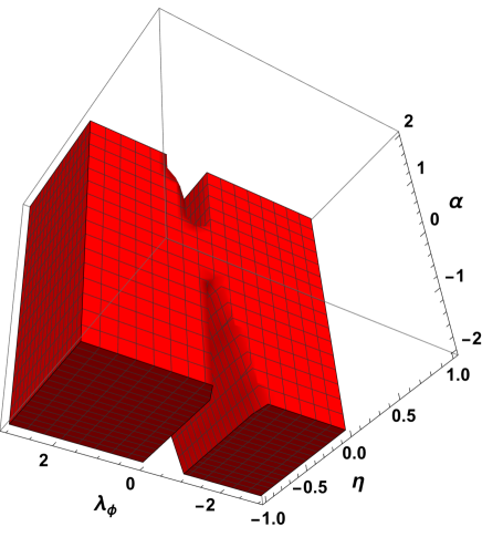
Figure 1: The figure displays a possible saddle region for the $P_{6}$ critical point ($\lambda_{\sigma}=2$).

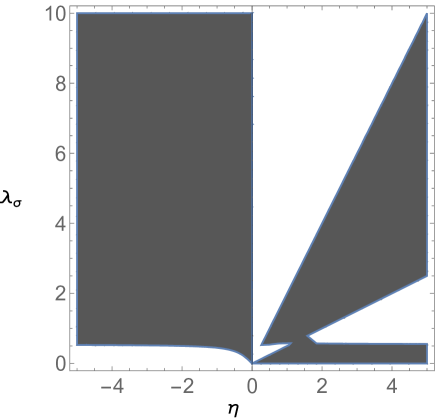
Figure 2: A non–exclusive saddle region for the $P_{7}$ solution where the de–Sitter behavior is expected ($w_{m}=0$).

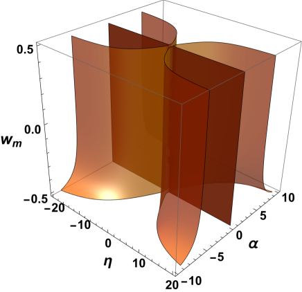
Figure 3: A non–exclusive region for the $P_{9}$ solution where the matter density parameter is $s=0.3$.

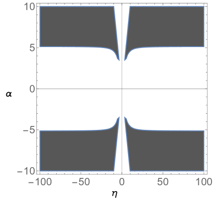
Figure 4: A non–exclusive region where the $P_{9}$ solution is saddle ($w_{m}=0,\lambda_{\phi}=1,\lambda_{\sigma}=1$).

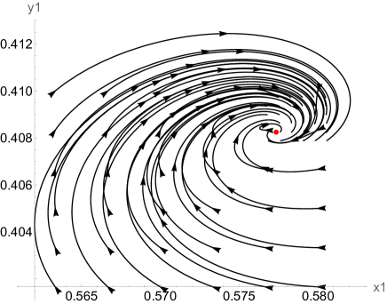
Figure 5: The evolution near the $P_{11}$ critical point (represented as a red dot) in the $Ox_{1}y_{1}$ plane ($w_{m}=0,\lambda_{\phi}=3,\lambda_{\sigma}=1,\eta=1,\alpha=1$).

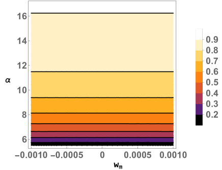
Figure 6: The matter density parameter for the $P_{13}$ cosmological solution.

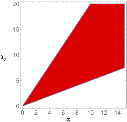
Figure 7: A region of interest for the $P_{14}$ cosmological solution where the dynamics corresponds to a saddle behavior ($w_{m}=0$).

3 Dynamical properties for a quintom scenario

In this section we shall investigate the dynamical properties of the present cosmological model by considering that we have a quintom scenario with $\epsilon_{1}=+1,\epsilon_{2}=-1$. In this case the $\phi$ component is associated to the quintessence, while the $\sigma$ term describes a non–canonical field with a negative kinetic energy violating various aspects from a physical point of view. The dynamical aspects are investigated by adopting the linear stability theory, an important tool in modern cosmology. In order to study the dynamical features, we introduce the following dimensionless variables:

$$x_{1}=\frac{\dot{\phi}}{H\sqrt{3}},$$ (22)

$$x_{2}=\frac{\dot{\sigma}}{H\sqrt{3}},$$ (23)

$$y_{1}=\frac{\sqrt{V_{1}(\phi)}}{H\sqrt{3}},$$ (24)

$$y_{2}=\frac{\sqrt{V_{2}(\sigma)}}{H\sqrt{3}},$$ (25)

$$z_{1}=2\beta f(\phi)H^{4},$$ (26)

$$z_{2}=2\beta g(\sigma)H^{4},$$ (27)

$$s=\frac{\rho_{m}}{3H^{2}}.$$ (28)

For the potential energy terms we shall consider the exponential decomposition,

$$V_{1}(\phi)=V_{10}e^{-\lambda_{\phi}\phi},$$ (29)

$$V_{2}(\sigma)=V_{20}e^{-\lambda_{\sigma}\sigma},$$ (30)

where $V_{10},V_{20},\lambda_{\phi}$ and $\lambda_{\sigma}$ are constant positive parameters. Furthermore, for the coupling functions we have taken:

$$f(\phi)=f_{0}e^{\alpha\phi},$$ (31)

$$g(\sigma)=g_{0}e^{\eta\sigma},$$ (32)

with $f_{0},g_{0},\alpha,\eta$ constant parameters associated to the strength of the cubic dependence.

In order to study the physical features of the phase space structure, we shall introduce a new variable $N=log(a)$, approximating the evolution of our cosmological model by an autonomous system of differential equations. In this case we shall obtain the following autonomous system:

$$\frac{dx_{1}}{dN}=-x_{1}\frac{\dot{H}}{H^{2}}+\frac{\ddot{\phi}}{\sqrt{3}H^{2}},$$ (33)

$$\frac{dx_{2}}{dN}=-x_{2}\frac{\dot{H}}{H^{2}}+\frac{\ddot{\sigma}}{\sqrt{3}H^{2}},$$ (34)

$$\frac{dy_{1}}{dN}=-y_{1}\frac{\dot{H}}{H^{2}}-\frac{\sqrt{3}}{2}\lambda_{\phi}x_{1}y_{1},$$ (35)

$$\frac{dy_{2}}{dN}=-y_{2}\frac{\dot{H}}{H^{2}}-\frac{\sqrt{3}}{2}\lambda_{\sigma}x_{2}y_{2},$$ (36)

$$\frac{dz_{1}}{dN}=4z_{1}\frac{\dot{H}}{H^{2}}+\sqrt{3}\alpha x_{1}z_{1},$$ (37)

$$\frac{dz_{1}}{dN}=4z_{2}\frac{\dot{H}}{H^{2}}+\sqrt{3}\eta x_{2}z_{2}.$$ (38)

Then, the Friedmann constraint equation reduces to:

$$s=3\sqrt{3}\alpha x_{1}z_{1}+3\sqrt{3}\eta x_{2}z_{2}-\frac{x_{1}^{2}}{2}+\frac{x_{2}^{2}}{2}-y_{1}^{2}-y_{2}^{2}-z_{1}-z_{2}+1.$$ (39)

In order to close the autonomous system we need to rewrite the Klein–Gordon equations in terms of auxiliary variables, obtaining:

$$\ddot{\phi}=-3\sqrt{3}H^{2}x_{1}+3H^{2}y_{1}^{2}\lambda_{\phi}+6\alpha H^{2}z_{1}+9\alpha z_{1}\dot{H},$$ (40)

$$\ddot{\sigma}=-3\sqrt{3}H^{2}x_{2}-3H^{2}y_{2}^{2}\lambda_{\sigma}-6\eta H^{2}z_{2}-9\eta z_{2}\dot{H}.$$ (41)

Lastly, the second Friedmann equation, the acceleration relation reduces to the following expression:

$$-3H^{2}-2\dot{H}=3H^{2}sw_{m}+9\alpha^{2}H^{2}x_{1}^{2}z_{1}+6\sqrt{3}\alpha H^{2}x_{1}z_{1}\\ +9\eta^{2}H^{2}x_{2}^{2}z_{2}+6\sqrt{3}\eta H^{2}x_{2}z_{2}+\frac{3}{2}H^{2}x_{1}^{2}-\frac{3}{2}H^{2}x_{2}^{2}-3H^{2}y_{1}^{2}\\ -3H^{2}y_{2}^{2}-3H^{2}z_{1}-3H^{2}z_{2}+12\sqrt{3}\alpha x_{1}z_{1}\dot{H}+12\sqrt{3}\eta x_{2}z_{2}\dot{H}\\ -6z_{1}\dot{H}-6z_{2}\dot{H}+3\alpha z_{1}\ddot{\phi}+3\eta z_{2}\ddot{\sigma},$$ (42)

closing the system of differential equations in an autonomous manner. For the system of equations (33)–(38) we have identified various critical points which are associated to different cosmological epochs. In what follows we shall discuss the obtained results and the corresponding dynamical features.

The first critical point represents the origin of the phase space structure, located at the following coordinates:

$$O:=[x_{1}=0,x_{2}=0,y_{1}=0,y_{2}=0,z_{1}=0,z_{2}=0],$$ (43)

where the total equation of state corresponds to a matter era ($w_{tot}=w_{m},s=1$), with the following eigenvalues:

$$\Big{[}\frac{3}{2}\left(w_{m}-1\right),\frac{3}{2}\left(w_{m}-1\right),-6\left(w_{m}+1\right),-6\left(w_{m}+1\right),\\ \frac{3}{2}\left(w_{m}+1\right),\frac{3}{2}\left(w_{m}+1\right)\Big{]}.$$ (44)

In the case where $w_{m}\to 0$ the solution is associated to a saddle dynamical behavior, describing the late matter epoch.

The second solution is located to the following coordinates:

$$P_{1}^{\pm}:=[x_{2}=\pm\sqrt{x_{1}^{2}-2},y_{1}=0,y_{2}=0,z_{1}=0,z_{2}=0],$$ (45)

describing a critical line which is related to the kinetic variables of the two scalar fields. This solution appears also in the minimally coupled case, describing a stiff fluid solution ($w_{tot}=1,s=0$), a particular representation which is not of great interest nowadays. The corresponding eigenvalues are the following:

$$\Big{[}0,3-3w_{m},\sqrt{3}\alpha x_{1}-12,3-\frac{1}{2}\sqrt{3}x_{1}\lambda_{\phi},\pm\sqrt{3}\eta\sqrt{x_{1}^{2}-2}-12,\\ \mp\frac{1}{2}\sqrt{3}\sqrt{x_{1}^{2}-2}\lambda_{\sigma}+3\Big{]}.$$ (46)

Since the second eigenvalue is always positive when $w_{m}\to 0$ this solution cannot be stable, it is either saddle or unstable. Moreover, the solution is non-hyperbolic due to the existence of a zero eigenvalue. Due to this aspect, the linear stability theory can be used only to constrain and study the saddle characteristics, a feature which is particular for two-field dark energy models.

The third cosmological solution is represented by a de–Sitter ($w_{tot}=-1,s=0$) epoch located at the following coordinates:

$$P_{2}:=[x_{1}=0,x_{2}=0,y_{1}=\frac{\sqrt{2}\sqrt{-\alpha}\sqrt{z_{1}}}{\sqrt{\lambda_{\phi}}},\\ y_{2}=\frac{\sqrt{2}\sqrt{\eta\lambda_{\phi}+2\alpha\eta z_{1}-\eta z_{1}\lambda_{\phi}}}{\sqrt{2\eta\lambda_{\phi}-\lambda_{\sigma}\lambda_{\phi}}},\\ z_{2}=\frac{-\lambda_{\sigma}\lambda_{\phi}-2\alpha z_{1}\lambda_{\sigma}+z_{1}\lambda_{\sigma}\lambda_{\phi}}{\lambda_{\phi}\left(2\eta-\lambda_{\sigma}\right)}],$$ (47)

describing a cosmological solution where the two dark energy fields are at rest without any kinetic energy. The dynamics is driven by the potential energy terms, and the strength of the cubic couplings embedded into $\alpha,\eta$ coefficients. However, due to the high complexity of the phase space structure, we haven’t been able to find the corresponding eigenvalues in the most general case. Hence, in order to check the stability of the cosmological solution, we have set the parameters to the following values: $w_{m}=0,\alpha=-1,\eta=1,\lambda_{\phi}=1,\lambda_{\sigma}=1,z_{1}=1$, obtaining the eigenvalues $\approx[0.,-3.,-3.95+0.85i,0.95\,-0.85i,-3.95-0.85i,0.95\,+0.85i]$ which are associated to a saddle dynamical behavior. In this case the accelerated expansion can be associated to this cosmological solution, describing a possible early dark energy where the fields are asymptotically frozen, without kinetic energy.

Next, the $P_{3}^{\pm}$ critical points are located at the coordinates:

$$P_{3}^{\pm}:=[x_{1}=\pm\frac{\sqrt{2}\sqrt{\eta^{2}+24}}{\eta},x_{2}=\frac{4\sqrt{3}}{\eta},y_{1}=0,y_{2}=0,\\ z_{1}=0,z_{2}=0],$$ (48)

with the corresponding eigenvalues:

$$\Big{[}0,0,3-3w_{m},\pm\frac{\sqrt{6}\alpha\sqrt{\eta^{2}+24}}{\eta}-12,3-\frac{6\lambda_{\sigma}}{\eta},\\ 3\mp\frac{\sqrt{\frac{3}{2}}\sqrt{\eta^{2}+24}\lambda_{\phi}}{\eta}\Big{]}.$$ (49)

These solutions are associated to a stiff–fluid case ($w_{tot}=1,s=0$) where the dark energy fluid completely dominates in terms of density parameters. As previously stated, these solutions are not of great interest for the modern cosmology, representing a not so feasible epoch driven only by the kinetic energies of the two scalar fields.

Furthermore, the $P_{4}^{\pm}$ solutions are located in the phase space structure at the coordinates:

$$P_{4}^{\pm}:=[x_{1}=\pm\frac{\sqrt{2}\sqrt{\lambda_{\sigma}^{2}+6}}{\lambda_{\sigma}},x_{2}=\frac{2\sqrt{3}}{\lambda_{\sigma}},y_{1}=0,y_{2}=0,\\ z_{1}=0,z_{2}=0],$$ (50)

where the corresponding eigenvalues are:

$$\Big{[}0,0,\frac{6\eta}{\lambda_{\sigma}}-12,3-3w_{m},\pm\frac{\sqrt{6}\alpha\sqrt{\lambda_{\sigma}^{2}+6}}{\lambda_{\sigma}}-12,\\ 3\mp\frac{\sqrt{\frac{3}{2}}\sqrt{\lambda_{\sigma}^{2}+6}\lambda_{\phi}}{\lambda_{\sigma}}\Big{]}.$$ (51)

As in the previous case, these stiff–fluid solutions ($w_{tot}=1,s=0$) describe an era where the expansion is not accelerated, with the dynamics driven only by the kinetic energy of the scalar fields.

The $P_{5}$ critical point located at:

$$P_{5}:=[x_{1}=0,x_{2}=-\frac{\lambda_{\sigma}}{\sqrt{3}},y_{1}=0,y_{2}=\frac{\sqrt{\lambda_{\sigma}^{2}+6}}{\sqrt{6}},\\ z_{1}=0,z_{2}=0],$$ (52)

represents a phantom solution where the effective equation of state is equal to:

$$w_{tot}=-\frac{\lambda_{\sigma}^{2}}{3}-1,$$ (53)

with the density parameter of the matter component equal to zero, describing a super accelerated expansion. For this solution we have obtained the following eigenvalues:

$$\Big{[}-\frac{\lambda_{\sigma}^{2}}{2},2\lambda_{\sigma}^{2},\lambda_{\sigma}\left(2\lambda_{\sigma}-\eta\right),\\ -\frac{\lambda_{\sigma}^{2}}{2}-3,-\frac{\lambda_{\sigma}^{2}}{2}-3,-\lambda_{\sigma}^{2}-3w_{m}-3\Big{]},$$ (54)

corresponding to an era which is always saddle from a dynamical perspective.

Next, the $P_{6}$ critical point (in the case when $w_{m}=0$) is located at the coordinates:

$$P_{6}:=[x_{1}=\frac{\sqrt{3}}{\lambda_{\phi}},x_{2}=\frac{2\sqrt{3}}{\eta},\\ y_{1}=\frac{\sqrt{\frac{3}{2}}\sqrt{\left(\left(\eta^{2}-4\right)\lambda_{\phi}^{2}+\eta^{2}\right)\left(5\eta^{2}\left(5\lambda_{\phi}^{2}+12\right)-366\lambda_{\phi}^{2}\right)}}{\sqrt{\lambda_{\phi}^{2}\left(\left(\eta^{2}-4\right)\lambda_{\phi}^{2}+\eta^{2}\right)\left(5\eta^{2}\left(5\lambda_{\phi}^{2}+12\right)-366\lambda_{\phi}^{2}\right)}},\\ y_{2}=0,z_{1}=0,z_{2}=\frac{6}{5\eta^{2}}]$$

represents a scaling solution Uzan:1999ch ; Marciu:2017sji where the effective equation of state is equal to:

$$w_{tot}=w_{m},$$ (55)

with the density parameter of the matter component:

$$s=\frac{132}{5\eta^{2}}-\frac{3}{\lambda_{\phi}^{2}}+1.$$ (56)

For this solution we have obtained the following eigenvalues:

$$\Big{[}\frac{3\left(\eta-2\lambda_{\sigma}\right)}{2\eta},-\frac{3\left(2\lambda_{\phi}-\alpha\right)}{\lambda_{\phi}},X_{3},X_{4},X_{5},X_{6}\Big{]}.$$ (57)

In this case the last eigenvalues ($X_{3}-X_{6}$) are not written in the manuscript due to the high complexity of the formulas involved. This scaling solution is important in the phase space structure since it can explain the matter epoch. As can be noted, the kinetic energies of the two fields are set to very specific values, while the potential energy of the $\phi$ field is influenced by $\lambda_{\phi}$ and $\eta$ parameters. Moreover, the strength of the cubic coupling for the $\sigma$ field is affected by the values of the $\eta$ constant parameter in a self–interacting manner. In Fig. 1 we have displayed a possible saddle region for the $P_{6}$ critical point by analyzing the signs of the first and second eigenvalues, considering that the first eigenvalue is positive, while the second eigenvalue is negative. As can be suspected, this analysis is not exclusive and only displays a possible region of interest associated to a saddle dynamical behavior where the two scalar fields are triggering a matter epoch, representing a scaling solution.

The $P_{7}$ solution, located at the coordinates:

$$P_{7}:=[x_{1}=0,x_{2}=0,y_{1}=0,y_{2}=\frac{\sqrt{2}\sqrt{\eta}}{\sqrt{2\eta-\lambda_{\sigma}}},z_{1}=0,\\ z_{2}=\frac{\lambda_{\sigma}}{\lambda_{\sigma}-2\eta}],$$

corresponds to a de–Siter era ($w_{tot}=-1,s=0$) where the two scalar fields are at rest without any kinetic energy, while the dynamics is driven by the potential energy of the $\sigma$ field, and its cubic coupling term. The corresponding eigenvalues are $[0,0,-3,X_{4},X_{5},X_{6}]$, where the last three terms are not displayed due to the complicated expressions involved. As can be observed, this critical point is non–hyperbolic and can be analyzed only in the saddle behavior using the linear stability theory. For this solution, we have displayed in Fig. 2 an interval associated to a saddle dynamical behavior, considering also the existence conditions which require that the $y_{2}$ variable is real and positive. This behavior mimics a cosmological constant dynamics and is expected to drive the evolution of the Universe in the future.

The $P_{8}^{\pm}$ solutions are found in the phase space structure at:

$$P_{8}^{\pm}:=[x_{1}=\frac{4\sqrt{3}}{\alpha},x_{2}=\pm\frac{\sqrt{2}\sqrt{24-\alpha^{2}}}{\alpha},\\ y_{1}=0,y_{2}=0,z_{1}=0,z_{2}=0],$$ (58)

driven a stiff–fluid scenario ($w_{tot}=1,s=0$), with the eigenvalues:

$$\Big{[}0,0,3-3w_{m},\pm\frac{\sqrt{6}\sqrt{24-\alpha^{2}}\eta}{\alpha}-12,3\mp\frac{\sqrt{36-\frac{3\alpha^{2}}{2}}\lambda_{\sigma}}{\alpha},\\ 3-\frac{6\lambda_{\phi}}{\alpha}\Big{]}.$$ (59)

The next solution $P_{9}$ represents a scaling cosmological epoch ($w_{tot}=w_{m}$) located at the coordinates:

$$P_{9}:=[x_{1}=\frac{2\sqrt{3}\left(w_{m}+1\right)}{\alpha},x_{2}=\frac{2\sqrt{3}\left(w_{m}+1\right)}{\eta},\\ y_{1}=0,y_{2}=0,z_{1}=\frac{6\left(w_{m}^{2}-1\right)}{\alpha^{2}\left(9w_{m}+5\right)},z_{2}=-\frac{6\left(w_{m}^{2}-1\right)}{\eta^{2}\left(9w_{m}+5\right)}],$$ (60)

with the matter density parameter equal to:

It can be observed that for this solution the potential energy terms are absent, with the dynamics driven by the kinetic energies and the cubic components of the two scalar fields. In principle, the location in the phase space structure and the physical properties are affected by the matter component through the barotropic equation of state, and the two cubic couplings, embedded into $\eta$ and $\alpha$ parameters. For this solution we have displayed in Fig. 3 a possible contour where the value of the matter density parameter is set $(s=0.3)$, obtaining various values of the associated parameters. The eigenvalues corresponding to this solution are the following (assuming a pressure–less mater component):

$$\Big{[}-\frac{3\alpha\eta\left(\alpha^{2}\left(25\eta^{2}+504\right)-504\eta^{2}\right)^{2}+3\sqrt{17}\sqrt{\alpha^{2}\eta^{2}\left(\alpha^{2}\left(25\eta^{2}+504\right)-504\eta^{2}\right)^{4}}}{4\alpha\eta\left(\alpha^{2}\left(25\eta^{2}+504\right)-504\eta^{2}\right)^{2}},\\ \frac{3\sqrt{17}\sqrt{\alpha^{2}\eta^{2}\left(\alpha^{2}\left(25\eta^{2}+504\right)-504\eta^{2}\right)^{4}}-3\alpha\eta\left(\alpha^{2}\left(25\eta^{2}+504\right)-504\eta^{2}\right)^{2}}{4\alpha\eta\left(\alpha^{2}\left(25\eta^{2}+504\right)-504\eta^{2}\right)^{2}},\\ -\frac{3\alpha\eta\left(\alpha^{2}\left(25\eta^{2}+504\right)-504\eta^{2}\right)^{2}+3\sqrt{\alpha^{2}\eta^{2}\left(\alpha^{2}\left(25\eta^{2}+504\right)-504\eta^{2}\right)^{3}\left(\alpha^{2}\left(425\eta^{2}+11064\right)-11064\eta^{2}\right)}}{4\alpha\eta\left(\alpha^{2}\left(25\eta^{2}+504\right)-504\eta^{2}\right)^{2}},\\ \frac{3\sqrt{\alpha^{2}\eta^{2}\left(\alpha^{2}\left(25\eta^{2}+504\right)-504\eta^{2}\right)^{3}\left(\alpha^{2}\left(425\eta^{2}+11064\right)-11064\eta^{2}\right)}-3\alpha\eta\left(\alpha^{2}\left(25\eta^{2}+504\right)-504\eta^{2}\right)^{2}}{4\alpha\eta\left(\alpha^{2}\left(25\eta^{2}+504\right)-504\eta^{2}\right)^{2}},\\ \frac{3}{2}-\frac{3\lambda_{\sigma}}{\eta},\frac{3}{2}-\frac{3\lambda_{\phi}}{\alpha}\Big{]}.$$ (62)

We have displayed in Fig. 4 a possible region of interest for the $P_{9}$ solution associated to a saddle dynamical behavior which takes into account also the existence conditions.

The next critical point $P_{10}$ represents also a stiff-fluid solution ($w_{tot}=1,s=0$) found at the coordinates:

$$P_{10}^{\pm}:=[x_{1}=\frac{2\sqrt{3}}{\lambda_{\phi}},x_{2}=\pm\frac{\sqrt{2}\sqrt{6-\lambda_{\phi}^{2}}}{\lambda_{\phi}},\\ y_{1}=0,y_{2}=0,z_{1}=0,z_{2}=0],$$ (63)

with the following eigenvalues (in the case of $P_{10}^{+}$):

$$\Big{[}0,0,\frac{6\alpha}{\lambda_{\phi}}-12,3-3w_{m},\frac{\sqrt{6}\eta\sqrt{6-\lambda_{\phi}^{2}}}{\lambda_{\phi}}-12,\\ 3-\frac{\lambda_{\sigma}\sqrt{9-\frac{3\lambda_{\phi}^{2}}{2}}}{\lambda_{\phi}}\Big{]}.$$ (64)

In the case of a pressure–less matter component this solution cannot be stable, it is either saddle or unstable, a solution which is not very relevant from a cosmological point of view.

The $P_{11}$ solution is driven by the canonical field $\phi$,

$$P_{11}:=[x_{1}=\frac{\sqrt{3}\left(w_{m}+1\right)}{\lambda_{\phi}},x_{2}=0,\\ y_{1}=\frac{\sqrt{\frac{3}{2}}\sqrt{1-w_{m}^{2}}}{\lambda_{\phi}},y_{2}=0,z_{1}=0,z_{2}=0],$$ (65)

acting as a saddle matter epoch ($w_{tot}=w_{m}$), $s=\frac{\lambda_{\phi}^{2}-3w_{m}-3}{\lambda_{\phi}^{2}}$, with the following eigenvalues:

$$\Big{[}\frac{3}{2}\left(w_{m}-1\right),-6\left(w_{m}+1\right),\frac{3}{2}\left(w_{m}+1\right),\frac{3\left(w_{m}+1\right)\left(\alpha-2\lambda_{\phi}\right)}{\lambda_{\phi}},\\ \frac{3}{4}\left(-\frac{\sqrt{\lambda_{\phi}^{10}\left(w_{m}-1\right)\left(\lambda_{\phi}^{2}\left(9w_{m}+7\right)-24\left(w_{m}+1\right){}^{2}\right)}}{\lambda_{\phi}^{6}}+w_{m}-1\right),\\ \frac{3\left(\lambda_{\phi}^{6}\left(w_{m}-1\right)+\sqrt{\lambda_{\phi}^{10}\left(w_{m}-1\right)\left(\lambda_{\phi}^{2}\left(9w_{m}+7\right)-24\left(w_{m}+1\right){}^{2}\right)}\right)}{4\lambda_{\phi}^{6}}\Big{]}.$$ (66)

At this solution the kinetic energy of the canonical field $\phi$ is influenced by the matter equation of state, and the strength of the potential energy term, encoded into the $\lambda_{\phi}$ coefficient. As can be seen, this solution is always saddle. The evolution near the $P_{11}$ critical point is represented in Fig. 5 for specific initial conditions, showing the dynamics in the $Ox_{1}y_{1}$ plane.

Furthermore, the $P_{12}$ solution located at the coordinates:

$$P_{12}:=[x_{1}=\frac{\lambda_{\phi}}{\sqrt{3}},x_{2}=0,\\ y_{1}=\frac{\sqrt{6-\lambda_{\phi}^{2}}}{\sqrt{6}},y_{2}=0,z_{1}=0,z_{2}=0],$$ (67)

describes a possible epoch where the acceleration of the Universe corresponds to a quintessence regime since

$$w_{tot}=\frac{\lambda_{\phi}^{2}}{3}-1,s=0.$$ (68)

From a dynamical point of view we have obtained the following eigenvalues:

$$\Big{[}-2\lambda_{\phi}^{2},\frac{\lambda_{\phi}^{2}}{2},\lambda_{\phi}\left(\alpha-2\lambda_{\phi}\right),\\ \lambda_{\phi}^{2}-3w_{m}-3,\frac{1}{2}\left(\lambda_{\phi}^{2}-6\right),\frac{1}{2}\left(\lambda_{\phi}^{2}-6\right)\Big{]},$$ (69)

indicating an era which is always saddle affected in principal by the strength of the potential energy of the canonical scalar field.

Next, the $P_{13}$ critical point, located at the coordinates:

$$P_{13}:=[x_{1}=\frac{2\sqrt{3}\left(w_{m}+1\right)}{\alpha},x_{2}=0,\\ y_{1}=0,y_{2}=0,z_{1}=\frac{6\left(w_{m}^{2}-1\right)}{\alpha^{2}\left(9w_{m}+5\right)},z_{2}=0],$$ (70)

is describing a scaling solution ($w_{tot}=w_{m}$) triggered by the kinetic energy of the canonical scalar field $\phi$ and the associated cubic component, with the matter density parameter equal to:

$$s=\frac{5\alpha^{2}+3\left(3\alpha^{2}-74\right)w_{m}+54w_{m}^{3}-36w_{m}^{2}-132}{\alpha^{2}\left(9w_{m}+5\right)}.$$ (71)

If we assume the case of a pressure–less matter component ($w_{m}=0$), then we obtain the following eigenvalues:

$$\Big{[}-\frac{3}{2},-6,\frac{3}{2},\\ -\frac{3\left(\alpha\left(504-25\alpha^{2}\right)^{2}+\sqrt{\alpha^{2}\left(25\alpha^{2}-504\right)^{3}\left(425\alpha^{2}-11064\right)}\right)}{4\alpha\left(504-25\alpha^{2}\right)^{2}},\\ \frac{3\left(\sqrt{\alpha^{2}\left(25\alpha^{2}-504\right)^{3}\left(425\alpha^{2}-11064\right)}-\alpha\left(504-25\alpha^{2}\right)^{2}\right)}{4\alpha\left(504-25\alpha^{2}\right)^{2}},\frac{3}{2}-\frac{3\lambda_{\phi}}{\alpha}\Big{]},$$ (72)

corresponding to a solution which is always saddle from a dynamical point of view. For this solution we have displayed in Fig. 6 a specific region where the matter density parameter $s$ satisfies the existence conditions, showing the viability of such a scaling behavior.

Lastly, the $P_{14}$ solution found at the coordinates:

$$P_{14}:=[x_{1}=0,x_{2}=0,\\ y_{1}=\frac{\sqrt{2}\sqrt{\alpha}}{\sqrt{2\alpha-\lambda_{\phi}}},y_{2}=0,z_{1}\frac{\lambda_{\phi}}{\lambda_{\phi}-2\alpha},z_{2}=0],$$ (73)

is associated to a de–Sitter epoch ($w_{tot}=-1,s=0$) where the two scalar fields are frozen. The dynamics is affected in principle by the potential energy of the canonical scalar field $\phi$, and the specific cubic component. This solution is similar to the $P_{7}$ critical point, representing a non–hyperbolic case where two eigenvalues are equal to zero. Since the expressions for the last eigenvalues are very complex, they are not displayed in the manuscript. As in the previous case, we show in Fig. 7 a specific region of interest where such a cosmological solution is having a saddle dynamical behavior, acting closely as a cosmological constant.

4 Summary and Conclusions

In the present paper we have proposed a novel dark energy model in the theoretical framework of modified gravity theories. This model extends the fundamental Einstein–Hilbert action by adding two scalar fields non–minimally coupled in an independent manner to an invariant component which contains cubic contractions of the Riemann tensor. After proposing the action for the current cosmological model, we have obtained the modified Friedmann equations by taking the variation of the action with respect to the inverse metric. The remaining field equations, the Klein–Gordon relations are developed by taking the variation with respect to the two fields which are present in the proposed action. As expected, the cosmological model satisfies the continuity equation due to the specific form of the proposed action. The dynamical features of the model are investigated by adopting the linear stability theory considering that the two fields are describing a quintom scenario, where a scalar field has a positive kinetic term, while the second field is associated to a non–canonical behavior, with a negative kinetic component, violating various physical principles from a classical point of view. From a theoretical point of view the quintom models are associated to a non–classical behavior as effective approaches in the modified gravity theories, being supported by various observations in the recent past. The analysis showed that the phase space structure is very rich in terms of stationary points, a complexity which can be associated to various stages in the evolution of the Universe. To this regard, we have obtained different classes of critical points which are associated to various cosmological eras. The first class of stationary points is represented by the stiff fluid solutions, a category which is not very interesting from a cosmological point of view. A second class of stationary points is represented by the de–Sitter solutions, a specific category which can explain the accelerated expansion where the model behaves as a cosmological constant. In this case the constant equation of state corresponds to $-1$ and can explain the late time evolution of the total equation of state. The third class of stationary points is associated to the scaling behavior where the effective equation of state corresponds to a matter epoch, a special type of solutions which can explain the existence of the matter epoch without fine–tuning. The scaling solutions found in the analysis are represented by an epoch characterized by a constant equation of state where the model behaves as a matter fluid, a dynamics driven by one or two scalar fields. In this case, the physical features are influenced by the couplings with the specific invariant which contains the third order contractions of the Riemann tensor, particular scaling solutions in the current cosmological setup. From a cosmological type of view the existence of this type of solutions in the phase space structure is very important for the viability of the corresponding models. The fourth class of solutions is associated to a quintessence or phantom behavior and can delineate the late time acceleration of the Universe by fine–tuning various parameters of the present model. These solutions can explain the quintessence–like and the phantom–like eras, as well as the possible crossing of the phantom divide line in the recent past. From the above discussion it can be noted that the present cosmological model can explain various stages in the evolution of our Universe, explaining both early and late time evolution in the phase space structure, a viable model from a theoretical point of view at the level of background dynamics.

- (1) P. J. E. Peebles and B. Ratra, Rev. Mod. Phys. 75 (2003), 559-606 doi:10.1103/RevModPhys.75.559
- (2) T. M. C. Abbott et al. [DES], Phys. Rev. D 105 (2022) no.2, 023520 doi:10.1103/PhysRevD.105.023520
- (3) P. A. R. Ade et al. [Planck], Astron. Astrophys. 594 (2016), A13 doi:10.1051/0004-6361/201525830 [arXiv:1502.01589 [astro-ph.CO]].
- (4) F. Beutler, C. Blake, M. Colless, D. H. Jones, L. Staveley-Smith, L. Campbell, Q. Parker, W. Saunders and F. Watson, Mon. Not. Roy. Astron. Soc. 416 (2011), 3017-3032 doi:10.1111/j.1365-2966.2011.19250.x [arXiv:1106.3366 [astro-ph.CO]].
- (5) E. J. Copeland, M. Sami and S. Tsujikawa, Int. J. Mod. Phys. D 15 (2006), 1753-1936 doi:10.1142/S021827180600942X [arXiv:hep-th/0603057 [hep-th]].
- (6) S. Capozziello and M. De Laurentis, Phys. Rept. 509 (2011), 167-321 doi:10.1016/j.physrep.2011.09.003 [arXiv:1108.6266 [gr-qc]].
- (7) T. Clifton, P. G. Ferreira, A. Padilla and C. Skordis, Phys. Rept. 513 (2012), 1-189 doi:10.1016/j.physrep.2012.01.001 [arXiv:1106.2476 [astro-ph.CO]].
- (8) K. Bamba, S. Capozziello, S. Nojiri and S. D. Odintsov, Astrophys. Space Sci. 342 (2012), 155-228 doi:10.1007/s10509-012-1181-8 [arXiv:1205.3421 [gr-qc]].
- (9) S. Nojiri, S. D. Odintsov and V. K. Oikonomou, Phys. Rept. 692 (2017), 1-104 doi:10.1016/j.physrep.2017.06.001 [arXiv:1705.11098 [gr-qc]].
- (10) K. Koyama, Rept. Prog. Phys. 79 (2016) no.4, 046902 doi:10.1088/0034-4885/79/4/046902 [arXiv:1504.04623 [astro-ph.CO]].
- (11) S. Tsujikawa, Lect. Notes Phys. 800 (2010), 99-145 doi:10.1007/978-3-642-10598-2_3 [arXiv:1101.0191 [gr-qc]].
- (12) U. Kasper and H. J. Schmidt, Nuovo Cim. B 104 (1989), 563-574 doi:10.1007/BF02726164
- (13) S. Nojiri and S. D. Odintsov, eConf C0602061 (2006), 06 doi:10.1142/S0219887807001928 [arXiv:hep-th/0601213 [hep-th]].
- (14) S. Tsujikawa, Class. Quant. Grav. 30 (2013), 214003 doi:10.1088/0264-9381/30/21/214003 [arXiv:1304.1961 [gr-qc]].
- (15) R. R. Caldwell, M. Kamionkowski and N. N. Weinberg, Phys. Rev. Lett. 91 (2003), 071301 doi:10.1103/PhysRevLett.91.071301 [arXiv:astro-ph/0302506 [astro-ph]].
- (16) A. Vikman, Phys. Rev. D 71 (2005), 023515 doi:10.1103/PhysRevD.71.023515 [arXiv:astro-ph/0407107 [astro-ph]].
- (17) S. Nojiri, S. D. Odintsov and S. Tsujikawa, Phys. Rev. D 71 (2005), 063004 doi:10.1103/PhysRevD.71.063004 [arXiv:hep-th/0501025 [hep-th]].
- (18) K. J. Ludwick, Mod. Phys. Lett. A 32 (2017) no.28, 1730025 doi:10.1142/S0217732317300257 [arXiv:1708.06981 [astro-ph.CO]].
- (19) B. Feng, X. L. Wang and X. M. Zhang, Phys. Lett. B 607 (2005), 35-41 doi:10.1016/j.physletb.2004.12.071 [arXiv:astro-ph/0404224 [astro-ph]].
- (20) D. Huterer and A. Cooray, Phys. Rev. D 71 (2005), 023506 doi:10.1103/PhysRevD.71.023506 [arXiv:astro-ph/0404062 [astro-ph]].
- (21) S. Nesseris and L. Perivolaropoulos, Phys. Rev. D 72 (2005), 123519 doi:10.1103/PhysRevD.72.123519 [arXiv:astro-ph/0511040 [astro-ph]].
- (22) H. Mohseni Sadjadi and M. Alimohammadi, Phys. Rev. D 74 (2006), 043506 doi:10.1103/PhysRevD.74.043506 [arXiv:gr-qc/0605143 [gr-qc]].
- (23) M. Alimohammadi and H. M. Sadjadi, Phys. Lett. B 648 (2007), 113-118 doi:10.1016/j.physletb.2007.03.014 [arXiv:gr-qc/0608016 [gr-qc]].
- (24) Z. K. Guo, Y. S. Piao, X. Zhang and Y. Z. Zhang, Phys. Rev. D 74 (2006), 127304 doi:10.1103/PhysRevD.74.127304 [arXiv:astro-ph/0608165 [astro-ph]].
- (25) S. G. Shi, Y. S. Piao and C. F. Qiao, JCAP 04 (2009), 027 doi:10.1088/1475-7516/2009/04/027 [arXiv:0812.4022 [astro-ph]].
- (26) H. Wei and S. N. Zhang, Phys. Rev. D 76 (2007), 063005 doi:10.1103/PhysRevD.76.063005 [arXiv:0705.4002 [gr-qc]].
- (27) R. Lazkoz, G. Leon and I. Quiros, Phys. Lett. B 649 (2007), 103-110 doi:10.1016/j.physletb.2007.03.060 [arXiv:astro-ph/0701353 [astro-ph]].
- (28) G. Leon, A. Paliathanasis and J. L. Morales-Martínez, Eur. Phys. J. C 78 (2018) no.9, 753 doi:10.1140/epjc/s10052-018-6225-y [arXiv:1808.05634 [gr-qc]].
- (29) M. Marciu, Can. J. Phys. 99 (2021) no.4, 281-290 doi:10.1139/cjp-2020-0037
- (30) M. Marciu, Eur. Phys. J. C 80 (2020) no.9, 894 doi:10.1140/epjc/s10052-020-08476-9 [arXiv:2005.03443 [gr-qc]].
- (31) M. Marciu, F. V. Iancu, D. M. Ioan and V. Baran, Rom. J. Phys. 65 (2020) no.7-8, 115
- (32) M. Marciu, Phys. Rev. D 99 (2019) no.4, 043508 doi:10.1103/PhysRevD.99.043508
- (33) M. Marciu, D. M. Ioan and F. V. Iancu, Int. J. Mod. Phys. D 28 (2018) no.01, 1950018 doi:10.1142/S0218271819500184
- (34) S. Bahamonde, M. Marciu and P. Rudra, JCAP 04 (2018), 056 doi:10.1088/1475-7516/2018/04/056 [arXiv:1802.09155 [gr-qc]].
- (35) M. Marciu, Phys. Rev. D 93 (2016) no.12, 123006 doi:10.1103/PhysRevD.93.123006
- (36) P. Bueno and P. A. Cano, Phys. Rev. D 94 (2016) no.10, 104005 doi:10.1103/PhysRevD.94.104005 [arXiv:1607.06463 [hep-th]].
- (37) P. Bueno, P. A. Cano, R. A. Hennigar and R. B. Mann, Phys. Rev. Lett. 122 (2019) no.7, 071602 doi:10.1103/PhysRevLett.122.071602 [arXiv:1808.02052 [hep-th]].
- (38) P. Bueno, P. A. Cano and A. Ruipérez, JHEP 03 (2018), 150 doi:10.1007/JHEP03(2018)150 [arXiv:1802.00018 [hep-th]].
- (39) J. Jiang and B. Deng, Eur. Phys. J. C 79 (2019) no.10, 832 doi:10.1140/epjc/s10052-019-7339-6
- (40) M. C. Pookkillath, A. De Felice and A. A. Starobinsky, JCAP 07 (2020), 041 doi:10.1088/1475-7516/2020/07/041 [arXiv:2004.03912 [gr-qc]].
- (41) P. Bueno, P. A. Cano, V. S. Min and M. R. Visser, Phys. Rev. D 95 (2017) no.4, 044010 doi:10.1103/PhysRevD.95.044010 [arXiv:1610.08519 [hep-th]].
- (42) Y. Z. Li, H. Lu and J. B. Wu, Phys. Rev. D 97 (2018) no.2, 024023 doi:10.1103/PhysRevD.97.024023 [arXiv:1711.03650 [hep-th]].
- (43) R. A. Hennigar, M. B. J. Poshteh and R. B. Mann, Phys. Rev. D 97 (2018) no.6, 064041 doi:10.1103/PhysRevD.97.064041 [arXiv:1801.03223 [gr-qc]].
- (44) P. Bueno, P. A. Cano, J. Moreno and Á. Murcia, JHEP 11 (2019), 062 doi:10.1007/JHEP11(2019)062 [arXiv:1906.00987 [hep-th]].
- (45) E. Cáceres, R. Castillo Vásquez and A. Vilar López, JHEP 05 (2021), 186 doi:10.1007/JHEP05(2021)186 [arXiv:2009.11595 [hep-th]].
- (46) J. Beltrán Jiménez and A. Jiménez-Cano, JCAP 01 (2021), 069 doi:10.1088/1475-7516/2021/01/069 [arXiv:2009.08197 [gr-qc]].
- (47) J. D. Edelstein, N. Grandi and A. Rivadulla Sánchez, JHEP 05 (2022), 188 doi:10.1007/JHEP05(2022)188 [arXiv:2202.05781 [hep-th]].
- (48) P. Rudra, [arXiv:2206.03490 [gr-qc]].
- (49) C. Erices, E. Papantonopoulos and E. N. Saridakis, Phys. Rev. D 99 (2019) no.12, 123527 doi:10.1103/PhysRevD.99.123527 [arXiv:1903.11128 [gr-qc]].
- (50) M. Marciu, Phys. Rev. D 101 (2020) no.10, 103534 doi:10.1103/PhysRevD.101.103534 [arXiv:2003.06403 [gr-qc]].
- (51) I. Quiros, R. García-Salcedo, T. Gonzalez, J. L. M. Martínez and U. Nucamendi, Phys. Rev. D 102 (2020) no.4, 044018 doi:10.1103/PhysRevD.102.044018 [arXiv:2003.10516 [gr-qc]].
- (52) M. Marciu, Phys. Rev. D 102 (2020) no.2, 023517 doi:10.1103/PhysRevD.102.023517 [arXiv:2004.07120 [gr-qc]].
- (53) M. Marciu, [arXiv:2203.00598 [gr-qc]].
- (54) M. Marciu, Eur. Phys. J. C 81 (2021) no.12, 1084 doi:10.1140/epjc/s10052-021-09871-6 [arXiv:2103.08420 [gr-qc]].
- (55) K. Giri and P. Rudra, Nucl. Phys. B 978 (2022), 115746 doi:10.1016/j.nuclphysb.2022.115746 [arXiv:2107.12417 [astro-ph.CO]].
- (56) I. Quiros, R. De Arcia, R. García-Salcedo, T. Gonzalez, F. X. Linares Cedeño and U. Nucamendi, Phys. Rev. D 103 (2021) no.6, 064043 doi:10.1103/PhysRevD.103.064043 [arXiv:2007.06111 [gr-qc]].
- (57) J. D. Edelstein, D. Vázquez Rodríguez and A. Vilar López, JCAP 12 (2020), 040 doi:10.1088/1475-7516/2020/12/040 [arXiv:2006.10007 [hep-th]].
- (58) G. Arciniega, P. Bueno, P. A. Cano, J. D. Edelstein, R. A. Hennigar and L. G. Jaime, Int. J. Mod. Phys. D 28 (2019) no.14, 1944008 doi:10.1142/S0218271819440085
- (59) G. Arciniega, P. Bueno, P. A. Cano, J. D. Edelstein, R. A. Hennigar and L. G. Jaime, Phys. Lett. B 802 (2020), 135242 doi:10.1016/j.physletb.2020.135242 [arXiv:1812.11187 [hep-th]].
- (60) G. Arciniega, J. D. Edelstein and L. G. Jaime, Phys. Lett. B 802 (2020), 135272 doi:10.1016/j.physletb.2020.135272 [arXiv:1810.08166 [gr-qc]].
- (61) R. A. Hennigar and R. B. Mann, Phys. Rev. D 95 (2017) no.6, 064055 doi:10.1103/PhysRevD.95.064055 [arXiv:1610.06675 [hep-th]].
- (62) P. Bueno and P. A. Cano, Phys. Rev. D 94 (2016) no.12, 124051 doi:10.1103/PhysRevD.94.124051 [arXiv:1610.08019 [hep-th]].
- (63) X. H. Feng, H. Huang, Z. F. Mai and H. Lu, Phys. Rev. D 96 (2017) no.10, 104034 doi:10.1103/PhysRevD.96.104034 [arXiv:1707.06308 [hep-th]].
- (64) C. Adair, P. Bueno, P. A. Cano, R. A. Hennigar and R. B. Mann, Phys. Rev. D 102 (2020) no.8, 084001 doi:10.1103/PhysRevD.102.084001 [arXiv:2004.09598 [gr-qc]].
- (65) Y. F. Cai, E. N. Saridakis, M. R. Setare and J. Q. Xia, Phys. Rept. 493 (2010), 1-60 doi:10.1016/j.physrep.2010.04.001 [arXiv:0909.2776 [hep-th]].
- (66) J. P. Uzan, Phys. Rev. D 59 (1999), 123510 doi:10.1103/PhysRevD.59.123510 [arXiv:gr-qc/9903004 [gr-qc]].
- (67) M. Marciu, Int. J. Mod. Phys. D 26 (2017) no.09, 1750103 doi:10.1142/S0218271817501036
- (68) Wolfram Research, Inc., Mathematica, Champaign, IL, https://www.wolfram.com/mathematica.
- (69) J. M. Martin-Garcia, xAct: Efficient tensor computer algebra for the Wolfram Language, http://www.xact.es.