Abstract

In the Galaxy, extremely large mass-ratio inspirals(X-MRIs) composed of brown dwarfs and the massive black hole at the Galactic Center are expected to be promising gravitational wave sources for space-borne detectors. In this work, we simulate the gravitational wave signals from twenty X-MRI systems by an axisymmetric Konoplya-Rezzolla-Zhidenko metric with varied parameters. We find that the mass, spin, and deviation parameters of the Kerr black hole could be determined accurately ( $\sim 10^{-5}-10^{-6}$ ) with only one X-MRI event with a high signal-to-noise ratio. The measurement of the above parameters could be improved with more X-MRI observations.

1 1 0 https://doi.org/ Measurement of the central Galactic black hole by extremely large mass-ratio inspirals Title Shu-Cheng Yang ^1,†*, Huijiao Luo ^1,, Yuan-Hao Zhang ^2,3 and Chen Zhang ^1, Firstname Lastname, Firstname Lastname and Firstname Lastname Lastname, F.; Lastname, F.; Lastname, F. Correspondence: ysc@shao.ac.cn

1 Introduction

The first observations of gravitational waves(GWs) from binary black hole mergers and binary neutron star inspirals ushered in a new era of GW physics and astronomyB.P. Abbott et al. (2016) (The LIGO Scientific Collaboration and the Virgo Collaboration); B.P. Abbott et al. (2017) (The LIGO Scientific Collaboration and the Virgo Collaboration). Since then, the ground-based detectors have detected 90 GW eventsB.P. Abbott et al. (2019) (The LIGO Scientific Collaboration and the Virgo Collaboration); R. Abbott et al. (2021) (The LIGO Scientific Collaboration and the Virgo Collaboration, The LIGO Scientific Collaboration, the Virgo Collaboration, and the KAGRA Collaboration). The detectable frequency band of current ground-based GW detectors such as Advanced LIGOJ. Aasi et al. (2015) (The LIGO Scientific Collaboration), Advanced Virgo Acernese et al. (2014), and KAGRA The KAGRA Collaboration (2019) ranges from 10 to 10,000 Hz, which makes ground-based GW detectors unable to detect any GWs with frequencies less than 10 Hz, while abundant sources are emitting GWs in the low-frequency bandAmaro-Seoane et al. (2007). The space-borne GW detectors such as LISA Amaro-Seoane et al. (2017), Taiji Hu and Wu (2017), and TianQin Luo et al. (2016), which will be launched in the 2030s, will open GW windows from 0.1 mHz to 1 Hz, and are expected to probe the nature of astrophysics, cosmology, and fundamental physics.

One of the most essential and promising GW sources for space-borne GW detectors is the extreme-mass ratio inspiral (EMRI), which is formed when a massive black hole (MBH) captures a small compact object.Amaro-Seoane et al. (2007); Gair et al. (2010). The word "inspiral" here means the inspiralling process that the relatively lighter object gradually spirals in toward the MBH due to the emission of GWs. The small object should be compact to keep it from being tidally disrupted by the MBH so that it is unlikely to be a main-sequence star. The possible candidate could be a stellar-mass black hole(BH), neutron star, white dwarf, or other compact objects. The designed space-borne detectors will be sensitive to EMRIs that contain MBHs with the mass $10^{4}-10^{7}M_{\odot}$ and small compact objects with stellar mass, and the fiducial mass ratio will be $10^{3}-10^{6}$Chua et al. (2017).

Moreover, a special kind of EMRI, extremely large mass-ratio inspirals (X-MRIs) with a mass ratio of $q\sim 10^{8}$ also are potential sources for space-borne GW detectorsGourgoulhon et al. (2019); Amaro-Seoane (2019). The X-MRI system is formed when an MBH captures a brown dwarf (BD) with mass $\sim 10^{-2}~{}M_{\odot}$. Brown dwarfs are substellar objects with insufficient mass to sustain nuclear fusion and become main-sequence starsBurrows and Liebert (1993). Brown dwarfs are denser than main-sequence stars, and their Roche limit is closer to the horizon of MBH Freitag (2002); Gourgoulhon et al. (2019). Therefore, brown dwarfs could survive very close to the MBH.

The mass of BD is relatively tiny, so space-borne GW detectors like LISA could only observe X-MRIs nearby, especially X-MRIs at the Galactic Center(GC)Gourgoulhon et al. (2019); Amaro-Seoane (2019). The MBH of these X-MRIs, Sgr A*, is 8 kpc from the solar system, and its mass is about $4\times 10^{6}~{}M_{\odot}$ Eckart and Genzel (1996); Ghez et al. (1998, 2008); Genzel et al. (2010). A typical X-MRI at the GC covers $\sim 10^{8}$ cycles, which last millions of years in the LISA bandAmaro-Seoane (2019). Such X-MRI could have a relatively high SNR (more than 1000), and dozens of X-MRIs might be observed during the LISA mission periodAmaro-Seoane (2019). Therefore, the X-MRIs at the GC offers a natural laboratory for studying the properties of BH and testing theories of gravity.

In this paper, we simulate the GW signals of X-MRIs at GC to show how and to what extent the fine structure of Sgr A* could be figured. In general relativity(GR), according to the no-hair theorem, BHs are characterized by their masses, spins, and electric charges, and the Kerr metric is believed to be the metric that describes the space-time of BH. However, alternative theories of gravity predict hairy black holes Afrin et al. (2021) and other metrics that describe the space-time of BHKonoplya et al. (2016). The parameterized metrics are proposed to describe the space-time of non-Kerr black holes. In this paper, to describe the space-time of X-MRIs at GC, we use a model-independent parameterization metric, Konoplya-Rezzolla-Zhidenko metric(KRZ metric)Konoplya et al. (2016), which can describe metrics that is generic stationery and axisymmetric.

This paper is organized as follows, in section 2, we review the KRZ parametrization. In section 3, we introduce the "kludge" waveforms used in our work and simulate the GW signals emitted by X-MRIs at GC. In section 4, based on the simulated GW signals, we apply the Fisher matrix to these GWs and present the accuracy of parameter estimation of Sgr A* for future space-borne GW detectors. The conclusion and outlook are given in section5. Throughout this letter, we use natural units $(G=c=1)$, greek letters $(\mu,\nu,\sigma,...)$ stand for space-time indices, and Einstein summation is assumed.

2 KRZ prametrized metric

GR is the most accurate and concise theory of gravity by farR. Abbott et al. (2021) (The LIGO Scientific Collaboration, the Virgo Collaboration, and the KAGRA Collaboration). While in practice, there are quite a few other theories of gravity, whose predictions resemble general relativity’s, to be tested. In the framework of GR, the Schwarzschild or Kerr metric describes the space-time of uncharged BH. However, in modified and alternative theories of gravity, there are other possible solutions for the description of the space-time of BHsHu et al. (2022); Cao et al. (2022); Zhang et al. (2022); Yang et al. (2022); Zhang et al. (2021); Yi and Wu (2020). The predictions of different theories of gravity are different, so a universal and reasonable theory about the GWs of X-MRI should be model-independent.

In order to deal with numerous metrics of non-Kerr black holes, one may use the parameterized metric to describe the space-time of non-Kerr black holes. There are several model-independent frameworks, one of which parametrizes the most generic black hole geometry through a finite number of adjustable quantities and is known as Johannsen-Psaltis parametrization (J-P metric) Johannsen and Psaltis (2011). The J-P metric expresses deviations from general relativity in terms of a Taylor expansion in powers of $M/r$, where $M$ is the mass of BH and $r$ is the radial coordinate.The J-P parametrization is widely adopted, but it is not a robust and generic parametrization for rotating black holes Konoplya et al. (2016); Ni et al. (2016). Notably, the parametric axisymmetric J-P metric obtained from the Janis-Newman algorithm Drake and Szekeres (2000) does not cover all deviations from Kerr space-time.

Another model-independent parameterization metric  Konoplya et al. (2016); Jiang et al. (2015), KRZ metric, is based on a double expansion in both the polar and radial directions of a generic stationary and axisymmetric metric.The KRZ metric is effective in reproducing the space-time of three commonly used rotating black holes (Kerr, rotating dilationHorne and Horowitz (1992), and Einstein-dilaton-Gauss-Bonnet black holesCardoso et al. (2014)) with finite parameters (see Ref.Konoplya et al. (2016) for more details). According to KRZ parameterization, the space-time of any axisymmetric black hole with total mass $M$ and rotation parameter $a$ could be expressed in the following formKonoplya et al. (2016):

$$ds^{2} = -\frac{N^{2}-W^{2}\sin^{2}\theta}{K^{2}}dt^{2}-2Wr\sin^{2}\theta dtd\phi$$ (1)

$$+K^{2}r^{2}\sin^{2}\theta d\phi^{2}+S\left(\frac{B^{2}}{N^{2}}dr^{2}+r^{2}d\theta^{2}\right),$$

where Younsi et al. (2016)

$$S = \frac{\Sigma}{r^{2}}=1+\frac{a^{2}}{r^{2}}\cos^{2}\theta\ ,$$ (2)

$$\Sigma = r^{2}+a^{2}\cos^{2}\theta,$$ (3)

$N,B,W$,and $K$ are the functions of the radial and polar coordinates (expanded in term $\cos\theta$),

$$W = \sum_{i=0}^{\infty}\frac{W_{i}(r)(\cos\theta)^{i}}{S},$$ (4)

$$B = 1+\sum_{i=0}^{\infty}B_{i}(r)(\cos\theta)^{i},$$ (5)

$$N^{2} = \left(1-\frac{r_{0}}{r}\right)A_{0}(r)+\sum_{i=1}^{\infty}A_{i}(r)(\cos\theta)^{i},$$ (6)

$$K^{2} = 1+\frac{aW}{r}+\frac{a^{2}}{r^{2}}+\sum_{i=1}^{\infty}\frac{K_{i}(r)(\cos\theta)^{i}}{S},$$ (7)

with

$$B_{i}=b_{i0}\frac{r_{0}}{r}+\tilde{B_{i}}\frac{r_{0}^{2}}{r^{2}},$$ (8)

$$\tilde{B_{i}}\equiv\frac{b_{i1}}{1+\frac{xb_{i2}}{1+\frac{xb_{i3}}{1+...}}},$$ (9)

$$W_{i}=b_{i0}\frac{r_{0}^{2}}{r^{2}}+\tilde{B_{i}}\frac{r_{0}^{3}}{r^{3}},$$ (10)

$$\tilde{W_{i}}\equiv\frac{\omega_{i1}}{1+\frac{x\omega_{i2}}{1+\frac{x\omega_{i3}}{1+...}}},$$ (11)

$$K_{i>0}(r)=k_{i0}\frac{r_{0}^{2}}{r^{2}}+\tilde{K_{i}}\frac{r_{0}^{3}}{r^{3}},$$ (12)

$$\tilde{K_{i}}\equiv\frac{k_{i1}}{1+\frac{xk_{i2}}{1+\frac{xk_{i3}}{1+...}}},$$ (13)

$$A_{0}(r)=1-\epsilon_{0}\frac{r_{0}}{r}+(a_{00}-\epsilon)\frac{r_{0}^{2}}{r^{2}}+\frac{a^{2}}{r^{2}}+\tilde{A_{0}}\frac{r_{0}^{3}}{r^{3}},$$ (14)

$$A_{i>0}=K_{i}(r)+\epsilon_{i}\frac{r_{0}^{2}}{r^{2}}+a_{i0}\frac{r_{0}^{3}}{r^{3}}+\tilde{A_{i}}\frac{r_{0}^{4}}{r^{4}},\ \$$ (15)

$$\tilde{A_{i}}\equiv\frac{a_{i1}}{1+\frac{xa_{i2}}{1+\frac{xa_{i3}}{1+...}}},$$ (16)

where $x=1-{r_{0}}/{r}$, and $r_{0}$ is the radius of the black hole horizon in the equatorial plane. The metric (1) is characterized by the order of expansion in radial and polar directions. The parameters $a_{ij},b_{ij},\omega_{ij},k_{ij}$ (here $i=0,1,2,3...,j=1,2,3...$) are effectively independent. This is because one of these functions, $A_{i}(x),B_{i}(x),W_{i}(x)$ and $K_{i}(x)$, is fixed by coordinate choiceYounsi et al. (2016).

In the following, we present the parameterized metric with first-order radial expansion and second-order polar direction, which describe the space-time of a deformed Kerr black holeYounsi et al. (2016); Ni et al. (2016):

$$B = 1+\frac{\delta_{4}r_{0}^{2}}{r^{2}}+\frac{\delta_{5}r_{0}^{2}}{r^{2}}\cos^{2}\theta,$$ (17)

$$W = \frac{1}{\Sigma}\left[\frac{\omega_{00}r_{0}^{2}}{r^{2}}+\frac{\delta_{2}r_{0}^{3}}{r^{3}}+\frac{\delta_{3}r_{0}^{3}}{r^{3}}\cos^{2}\theta\right],$$ (18)

$$K^{2} = 1+\frac{aW}{r}+\frac{1}{\Sigma}\left(\frac{k_{00}r_{0}^{2}}{r^{2}}+\frac{k_{21}r_{0}^{3}}{r^{3}}\cos^{2}\theta\right),$$ (19)

$$N^{2} = \left(1-\frac{r_{0}}{r}\right)\left[1-\frac{\epsilon_{0}r_{0}}{r}+(k_{00}-\epsilon_{0})\frac{r_{0}^{2}}{r^{2}}+\frac{\delta_{1}r_{0}^{3}}{r^{3}}\right]$$ (20)

$$+\left[(k_{21}+a_{20})\frac{r_{0}^{3}}{r^{3}}+\frac{a_{21}r_{0}^{4}}{r^{4}}\right]\cos^{2}\theta,$$

The radius of the horizon and the Kerr parameter are

$$r_{0}=M+\sqrt{M^{2}-a^{2}},\ \ a=J/M,$$ (21)

where $J$ is the total angular momentum. For simplicity, here $M$ has one unit, i.e. $M=1$. One can obtain related variables and parameters from dimensionless quantity by scale transformationsZhou et al. (2022); Wang et al. (2021a, b, c); Wu et al. (2021); Sun et al. (2021): $tM\rightarrow t$, $rM\rightarrow r$, etc. The coefficient $r_{0}$, $a_{20}$, $a_{21}$, $\epsilon_{0}$, $k_{00}$, $k_{21}$ and $\omega_{00}$ in the KRZ metric can be expressed as followsNi et al. (2016); Xin et al. (2019)

$$r_{0} = 1+\sqrt{1-\tilde{a}^{2}},$$ (22)

$$a_{20} = \frac{2\tilde{a}^{2}}{r_{0}^{3}},$$ (23)

$$a_{21} = -\frac{\tilde{a}^{4}}{r_{0}^{4}}+\delta_{6},$$ (24)

$$\epsilon_{0} = \frac{2-r_{0}}{r_{0}},$$ (25)

$$\omega_{00} = \frac{2\tilde{a}}{r_{0}^{2}},$$ (26)

$$k_{00} = \frac{\tilde{a}^{2}}{r_{0}^{2}},$$ (27)

$$k_{21} = \tilde{a}^{4}/r_{0}^{4}-2\tilde{a}^{2}/r_{0}^{3}-\delta_{6},$$ (28)

$$k_{22} = -\tilde{a}^{2}/r_{0}^{2}+\delta_{7},$$ (29)

$$k_{23} = \tilde{a}^{2}/r_{0}^{2}+\delta_{8},$$ (30)

here $\tilde{a}=a/M$ stands for the spin parameter. The deformation parameters ${\delta_{j}}(j=1,2,...,8)$ represent the deviations from the Kerr metric. The physical meaning of these parameters could be summarized as follows: $\delta_{1}$ is related to deformation of $g_{tt}$; $\delta_{2},\delta_{3}$ are related to the rotational deformation of the metric; $\delta_{4},\delta_{5}$ are related to deformation of $g_{rr}$ and $\delta_{6}$ is related to the deformation of the event horizon (see Ref. Konoplya et al. (2016) for more details). The KRZ metric is an appropriate tool to measure the potential deviations from the Kerr metric. As a first order approximation, in this work we mainly consider $\delta_{1}$ and $\delta_{2}$.

3 Waveform model for KRZ black holes

Several waveform models can simulate the signal of EMRIHughes (2001); Barack and Cutler (2004); Drasco and Hughes (2006); Babak et al. (2007); Chua and Gair (2015); Chua et al. (2017). Among these models, the kludge model can generate waveforms quickly and have a 95% accuracy compared with the Teukolsky-based waveformsBabak et al. (2007). The kludge waveforms may be essential in searching for EMRIs/X-MRIs for future space-borne GW detectors. We employ the kludge waveforms to simulate X-MRI waveformsXin et al. (2019). Before presenting the results, we would like to review the structure and logic of the calculation. The calculation of waveforms can be summarized in the following steps:

• First, to consider the brown dwarf of the X-MRI as a point particle.

• Second, to use the given metric to calculate the particle’s trajectory by integrating the geodesic equations that contain the radiation flux.

• Finally, to use the quadrupole expression to get the GWs emitted from the system of the X-MRI.

To get the trajectory of the particle, we start by calculating the geodesics using the following equations:

$$\dot{u}^{\mu} = -\Gamma_{\rho\sigma}^{\mu}u^{\rho}u^{\sigma},$$ (31)

$$\dot{x}^{\mu} = u^{\mu},$$ (32)

where $x^{\mu}$ is the coordinate of the particle, ${u}^{\mu}$ is the 4-velocity, which satisfies

$$|u|=g_{\mu\nu}u^{\mu}u^{\nu}=-1\ ,$$ (33)

and $\Gamma_{\rho\sigma}^{\mu}$ are the Christoffel symbols. For stable bounded geodesics, the orbital eccentricity $e$ and semi-latus rectum $p$ can be defined by periastron $r_{p}$ and apastron $r_{a}$, and the inclination angle $\iota$ is defined in the Keplerian convention by:

$$e =\frac{r_{a}-r_{p}}{r_{a}+r_{p}}, p =\frac{2r_{a}r_{p}}{r_{a}+r_{p}}, \iota =\frac{\pi}{2}-\theta_{\mathbf{min}}.$$ (34)

where $\theta_{\mathbf{min}}$ is the minimum of $\theta$ along the geodesic. The geodesic may be specified by the parameters $(r_{a},r_{p},\theta_{\mathbf{min}})$, which fully describe the range of motion in the radial and polar coordinates. In this paper, we define $(e,p,\iota)$ from $(r_{a},r_{p},\theta_{\mathbf{min}})$ by the numerically generated trajectory.

In the background of Kerr metric, the geodesic can be described by the orbital energy $E$, the $z$ component of the orbital angular momentum $L_{z}$, and the Carter constant $Q$Xin et al. (2019). $E$ and $L_{z}$ still exist in the KRZ background, and take the form

$$E = -u_{t}=-g_{tt}u^{t}-g_{t\phi}u^{\phi}\ ,$$ (35)

$$L_{z} = u_{\phi}=g_{t\phi}u^{t}+g_{\phi\phi}u^{\phi}\ .$$ (36)

Strictly speaking, unlike the Kerr metric, the Carter constant $Q$ does not exist in the KRZ metric. While when considering the situations that are close to the Kerr metric, we use an approximate "Carter constant" Rüdiger (1981, 1983)

$$Q=L_{z}^{2}\tan^{2}\iota,$$ (37)

While the orbital constants $(E,L_{z},Q)$ in the above geodesic setup do not vary with time, it is convenient to work with alternative parametrizations of $(E,L_{z},Q)$. The relationship between $(r_{a},r_{p},\theta_{\mathbf{min}})$ and $(E,L_{z},Q)$ is given byChua et al. (2017)

$$P^{2}{|_{r=r_{a},\theta=\pi/2}}-[r^{2}+(L_{z}^{2}-aE)^{2}+Q]\Delta{|_{r=r_{a},\theta=\pi/2}}=0,\qquad$$ (38)

$$P^{2}{|_{r=r_{p},\theta=\pi/2}}-[r^{2}+(L_{z}^{2}-aE)^{2}+Q]\Delta{|_{r=r_{p},\theta=\pi/2}}=0,$$ (39)

$$Q=\cos^{2}\theta_{\rm min}\left[a^{2}(1-E^{2})+\left(\frac{L_{z}}{\sin\theta}\right)^{2}\right].$$ (40)

Because of the extreme mass ratio of X-MRI, the deviations from the geodesics due to radiation reaction should be small. While in this work, for accuracy, we consider the effect of radiation reaction, which is included by replacing the Eq. (31) with the following one

$$\frac{du^{\mu}}{d\tau}=-\Gamma_{\rho\sigma}^{\mu}u^{\rho}u^{\sigma}+\mathcal{F}^{\mu}$$ (41)

where the radiation force $\mathcal{F}^{\mu}$ is connected with the adiabatic radiation fluxes $(\dot{E},\dot{L_{z}},\dot{Q})$ as

$$\dot{E}u^{t}=-g_{tt}\mathcal{F}^{t}-g_{t\phi}\mathcal{F}^{\phi},$$ (42)

$$\dot{L_{z}}u^{t}=g_{t\phi}\mathcal{F}^{t}+g_{\phi\phi}\mathcal{F}^{\phi},$$ (43)

$$\dot{Q}u^{t}=2g_{\theta\theta}^{2}u^{\theta}\mathcal{F}^{\theta}+2\cos^{2}\theta^{2}a^{2}E\dot{E}+2\cos^{2}\theta\frac{L_{z}\dot{L_{z}}}{\sin^{2}\theta},$$ (44)

$$g_{\mu\nu}u^{\mu}\mathcal{F}^{\nu}=0.$$ (45)

Eq. (42) can be deduced by taking derivatives with respect to proper time in Eqs. (35)-(37). Integrating the geodesic equations that contain the radiation flux is crucial for calculating the particle’s trajectory. In this paper, due to the short integration time, we use the Runge-Kutta method. There are also several geometric numerical integration methods for integrating the equations of geodesics. Such as manifold correction schemesWang et al. (2016, 2018); Deng et al. (2020), extended phase space methodsLi and Wu (2017); Luo et al. (2017); Pan et al. (2021); Liu et al. (2016), explicit and implicit combined symplectic methodsMei et al. (2013a, b); Zhong et al. (2010), and explicit symplectic integratorsZhou et al. (2022); Wang et al. (2021a, b, c); Wu et al. (2021); Sun et al. (2021). For situations such as the long-term evolution of Hamiltonian systemsDeng et al. (2020), geometric numerical integration methods can be helpful.

Finally, after generating the trajectory, we turn to the third step – to calculate the gravitational waveforms. We start from transforming the Boyer-Lindquist coordinates $(t,r,\phi,\theta)$ into Cartesian coordinates $(t,x,y,z)$ using the relations:

$$t = t,$$ (46)

$$x = r\sin\theta\cos\phi,$$ (47)

$$y = r\sin\theta\sin\phi,$$ (48)

$$z = r\cos\theta.$$ (49)

Then we calculate the quadrupole expression (see Ref. Babak et al. (2007))

$$\bar{h}^{jk}(t,x)=\frac{2}{r}[\ddot{I}^{jk}(t^{{}^{\prime}})]_{t^{{}^{\prime}}=t-r},$$ (51)

$$I^{jk}(t^{{}^{\prime}})=\int x^{{}^{\prime}j}x^{{}^{\prime}k}T^{00}(t^{{}^{\prime}},x^{{}^{\prime}})d^{3}x^{{}^{\prime}},$$

where $I^{jk}(t^{{}^{\prime}})$ is the source’s mass quadrupole moment, $T^{00}$ is component of the energy-momentum tensor $T^{\mu\nu}(t^{{}^{\prime}},x^{{}^{\prime}})$, and $\bar{h}^{\mu\nu}=h^{\mu\nu}-\frac{1}{2}\eta^{\mu\nu}\eta^{\rho\sigma}h_{\rho\sigma}$ is the trace-reversed metric perturbation. Then we transform the waveform into the transverse-traceless gauge (see Ref. Babak et al. (2007) for more details)

$$h_{TT}^{jk}=\frac{1}{2}\begin{pmatrix}0&0&0\\ 0&h^{\Theta\Theta}-h^{\Phi\Phi}&2h^{\Theta\Phi}\\ 0&2h^{\Theta\Phi}&h^{\Phi\Phi}-h^{\Theta\Theta}\end{pmatrix}\ ,$$ (52)

with

$$h^{\Theta\Theta} = \cos^{2}\Theta\left[h^{xx}\cos^{2}\Phi+h^{xy}\sin 2\Phi+h^{yy}\sin^{2}\Phi\right]$$ (53)

$$+h^{zz}\sin^{2}\Theta-\sin 2\Theta\left[h^{xz}\cos\Phi+h^{yz}\sin\Phi\right],$$

$$h^{\Phi\Theta} = \cos\Theta\left[-\frac{1}{2}h^{xx}\sin 2\Phi+h^{xy}\cos 2\Phi+\frac{1}{2}h^{yy}\sin 2\Phi\right]$$ (54)

$$+\sin\Theta\left[h^{xz}\sin\Phi-h^{yz}\cos\Phi\right],$$

$$h^{\Phi\Phi} = \left[h^{xx}\sin^{2}\Phi-h^{xy}\sin 2\Phi+h^{yy}\cos^{2}\Phi\right].$$ (55)

Now we get the plus and cross components of the waveform observed at latitudinal angle $\Theta$ and azimuthal angle $\Phi$

$$h_{+} = h^{\Theta\Theta}-h^{\Phi\Phi}$$ (56)

$$= \cos^{2}\Theta\left[h^{xx}\cos^{2}\Phi+h^{xy}\sin 2\Phi+h^{yy}\sin^{2}\Phi\right]$$

$$+h^{zz}\sin^{2}\Theta-\sin 2\Theta\left[h^{xz}\cos\Phi+h^{yz}\sin\Phi\right]$$

$$-\left[h^{xx}\sin^{2}\Phi-h^{xy}\sin 2\Phi+h^{yy}\cos^{2}\Phi\right],$$

$$h_{\times} = 2h^{\Theta\Phi}$$ (57)

$$= 2\Big{\{}\cos\Theta\left[-\frac{1}{2}h^{xx}\sin 2\Phi+h^{xy}\cos 2\Phi+\frac{1}{2}h^{yy}\sin 2\Phi\right]$$

$$+\sin\Theta\left[h^{xz}\sin\Phi-h^{yz}\cos\Phi\right]\Big{\}}.$$

The strength of the signal in a detector could be characterized by the signal-to-noise ratio (SNR). The SNR of the signals can be defined asFinn (1992)

$$\rho:=\sqrt{\left\langle h|h\right\rangle},$$ (58)

where $\left\langle\cdot|\cdot\right\rangle$ is the standard matched-filtering inner product between two data streams. The inner product between signal $a(t)$ and template $b(t)$ is

$$\left\langle a|b\right\rangle=2\int_{0}^{\infty}\frac{\tilde{a}^{*}(f)\tilde{b}(f)+{\tilde{a}(f)\tilde{b}^{*}(f)}}{S_{n}(f)}df$$ (59)

where $\tilde{a}(f)$ is the Fourier transform of the time series signal $a(t)$, $\tilde{a}^{*}(f)$ is the complex conjugate of $\tilde{a}(f)$ and $S_{n}(f)$ is the power spectral density of the GW detectors’ noise. Throughout this paper, the power spectral density is taken to be the noise level of LISA.

In this work, to quantify the differences between GW signals and the templates, we use maximized fitting factor (overlap)

$$\mathrm{FF}(a,b)=\frac{(a|b)}{\sqrt{(a|a)(b|b)}}.$$ (60)

If we include the time shift $t_{s}$ and the phase shift $\phi_{s}$, the fitting factor reads

$$\mathrm{ff}(t_{s},\phi_{s},a(t),b(t))=\frac{(a(t)|b(t+t_{s})e^{i\phi_{s}})}{\sqrt{(a|a)(b|b)}},$$ (61)

the maximized fitting factor is defined as

$$\mathrm{FF}(a,b)=\underset{t_{s},\phi_{s}}{\mathbf{max}}\frac{(a(t)|b(t+t_{s})e^{i\phi_{s}})}{\sqrt{(a|a)(b|b)}}.$$ (62)

4 Data analysis

In this section, we first specify the main parameters values we used in this work. Then we use XSPEG, a software for generating GWs in the KRZ metric, provided by the authors of Ref. Xin et al. (2019) to calculate the gravitational waveforms and do some analysis. Finally, we employ the Fisher information matrix to evaluate the parameter estimation accuracy for LISA-like GW detectors.

For X-MRI at the GC, the mass of the brown dwarfs ranges from $\sim 0.01~{}\rm M_{\odot}$ to $\sim 0.08~{}\rm M_{\odot}$ Chabrier and Baraffe (2000). The parameter values for the MBH Sgr A* in this work are as follows:

• the mass of Sgr A* $M_{\rm SgrA*}=4\times 10^{6}~{}\rm{M_{\odot}}$Eckart and Genzel (1996); Ghez et al. (1998, 2008);

• the dimensionless spin parameter $a=0.5$ Shcherbakov et al. (2012);

• the distance between Sgr A* and the solar system $R_{p}=8.3$ kpc Eisenhauer et al. (2003);

• the latitudinal angle $\Theta=-29^{\circ}$ and the azimuthal angle $\Phi=266.417^{\circ}$ Menten et al. (1997).

Based on the parameters above, we first simulate the GW signals of twenty X-MRIs at the GC (see Table 1 ). The mass ratio $q$ ranges from $5\times 10^{7}$ to $4.0\times 10^{8}$, the orbit eccentricity $e$ ranges from $0.1$ to $0.8$, the semi-latus rectum $p$ ranges from $10.6$ to $50.0$, the inclination angle $\iota$ ranges from $-2\pi/3$ to $\pi/3$, and the duration of above signals is one year. Then, we calculate the overlaps between above GW signals and many GW series with varying parameters. Finally, we use the Fisher information matrix to provide the uncertainties of parameter estimations.

4.1 The overlaps between simulated GW signals of XMRIs and GW series with varying parameters

Signal	e	p	$\iota$	$M_{Object}$	SNR	$\Delta a/a$	$\Delta M/M$	$\Delta\delta_{1}$	$\Delta\delta_{2}$	$\Delta R_{p}/R_{p}$
$01$	$0.617$	$10.600$	$5\pi/6$	$2.80\times 10^{-2}$	$1584.363$	$2.85\times 10^{-6}$	$4.18\times 10^{-7}$	$3.63\times 10^{-6}$	$3.28\times 10^{-6}$	$7.18\times 10^{-4}$
$02$	$0.520$	$12.000$	$\pi/6$	$2.00\times 10^{-2}$	$636.988$	$2.10\times 10^{-6}$	$9.53\times 10^{-7}$	$1.48\times 10^{-5}$	$1.48\times 10^{-5}$	$1.78\times 10^{-3}$
$03$	$0.300$	$14.400$	$\pi/6$	$2.00\times 10^{-2}$	$224.915$	$9.39\times 10^{-6}$	$4.04\times 10^{-6}$	$3.92\times 10^{-5}$	$4.95\times 10^{-5}$	$5.03\times 10^{-3}$
$04$	$0.200$	$16.800$	$\pi/7$	$2.72\times 10^{-2}$	$144.765$	$4.60\times 10^{-5}$	$4.54\times 10^{-6}$	$7.31\times 10^{-5}$	$1.04\times 10^{-4}$	$7.37\times 10^{-3}$
$05$	$0.400$	$16.800$	$\pi/7$	$2.72\times 10^{-2}$	$201.217$	$1.33\times 10^{-5}$	$2.91\times 10^{-6}$	$6.17\times 10^{-5}$	$8.26\times 10^{-5}$	$5.29\times 10^{-3}$
$06$	$0.514$	$27.243$	$-\pi/12$	$1.80\times 10^{-2}$	$30.518$	$2.47\times 10^{-4}$	$1.96\times 10^{-5}$	$8.48\times 10^{-4}$	$1.39\times 10^{-3}$	$3.58\times 10^{-2}$
$07$	$0.500$	$24.750$	$\pi/4$	$3.60\times 10^{-2}$	$59.061$	$7.79\times 10^{-5}$	$3.33\times 10^{-6}$	$1.70\times 10^{-4}$	$3.44\times 10^{-4}$	$1.68\times 10^{-2}$
$08$	$0.600$	$19.200$	$\pi/5$	$2.80\times 10^{-2}$	$148.460$	$1.92\times 10^{-5}$	$1.91\times 10^{-6}$	$1.21\times 10^{-4}$	$1.92\times 10^{-4}$	$6.92\times 10^{-3}$
$09$	$0.700$	$15.300$	$\pi/6$	$1.00\times 10^{-2}$	$140.487$	$1.15\times 10^{-5}$	$4.43\times 10^{-6}$	$1.54\times 10^{-4}$	$1.80\times 10^{-4}$	$7.73\times 10^{-3}$
$10$	$0.800$	$12.600$	$\pi/8$	$1.20\times 10^{-2}$	$355.391$	$4.80\times 10^{-6}$	$3.42\times 10^{-6}$	$6.45\times 10^{-5}$	$6.18\times 10^{-5}$	$3.27\times 10^{-3}$
$11$	$0.100$	$39.600$	$-\pi/6$	$7.00\times 10^{-2}$	$32.112$	$5.38\times 10^{-3}$	$6.25\times 10^{-5}$	$3.66\times 10^{-3}$	$9.96\times 10^{-3}$	$5.57\times 10^{-2}$
$12$	$0.253$	$35.093$	$-\pi/3$	$7.84\times 10^{-2}$	$39.303$	$7.72\times 10^{-5}$	$2.36\times 10^{-7}$	$4.13\times 10^{-5}$	$1.41\times 10^{-4}$	$2.63\times 10^{-2}$
$13$	$0.206$	$30.159$	$-\pi/4$	$7.60\times 10^{-2}$	$45.575$	$1.38\times 10^{-4}$	$1.94\times 10^{-6}$	$1.56\times 10^{-4}$	$3.69\times 10^{-4}$	$2.25\times 10^{-2}$
$14$	$0.368$	$41.053$	$-\pi/7$	$8.00\times 10^{-2}$	$47.910$	$1.49\times 10^{-3}$	$1.23\times 10^{-5}$	$3.00\times 10^{-3}$	$8.19\times 10^{-3}$	$3.61\times 10^{-2}$
$15$	$0.295$	$47.924$	$-\pi/9$	$6.00\times 10^{-2}$	$24.535$	$1.03\times 10^{-2}$	$1.18\times 10^{-4}$	$1.37\times 10^{-2}$	$3.34\times 10^{-2}$	$7.85\times 10^{-2}$
$16$	$0.425$	$32.775$	$-\pi/11$	$3.00\times 10^{-2}$	$19.701$	$6.08\times 10^{-4}$	$2.15\times 10^{-5}$	$1.04\times 10^{-3}$	$1.99\times 10^{-3}$	$5.27\times 10^{-2}$
$17$	$0.300$	$27.300$	$\pi/3$	$3.20\times 10^{-2}$	$27.179$	$9.05\times 10^{-5}$	$1.01\times 10^{-6}$	$7.17\times 10^{-5}$	$2.40\times 10^{-4}$	$3.78\times 10^{-2}$
$18$	$0.133$	$44.200$	$-2\pi/3$	$6.80\times 10^{-2}$	$29.731$	$9.80\times 10^{-4}$	$2.19\times 10^{-6}$	$4.83\times 10^{-4}$	$2.21\times 10^{-3}$	$3.43\times 10^{-2}$
$19$	$0.137$	$50.039$	$-\pi/3$	$7.20\times 10^{-2}$	$24.736$	$1.04\times 10^{-3}$	$2.53\times 10^{-6}$	$7.36\times 10^{-5}$	$2.42\times 10^{-3}$	$4.07\times 10^{-2}$
$20$	$0.477$	$25.108$	$-3\pi/5$	$8.00\times 10^{-2}$	$101.345$	$4.48\times 10^{-5}$	$2.05\times 10^{-7}$	$1.16\times 10^{-5}$	$3.58\times 10^{-5}$	$9.75\times 10^{-3}$

Table 1: Parameter setting and parameter estimation accuracy for the 20 X-MRIs at the GC

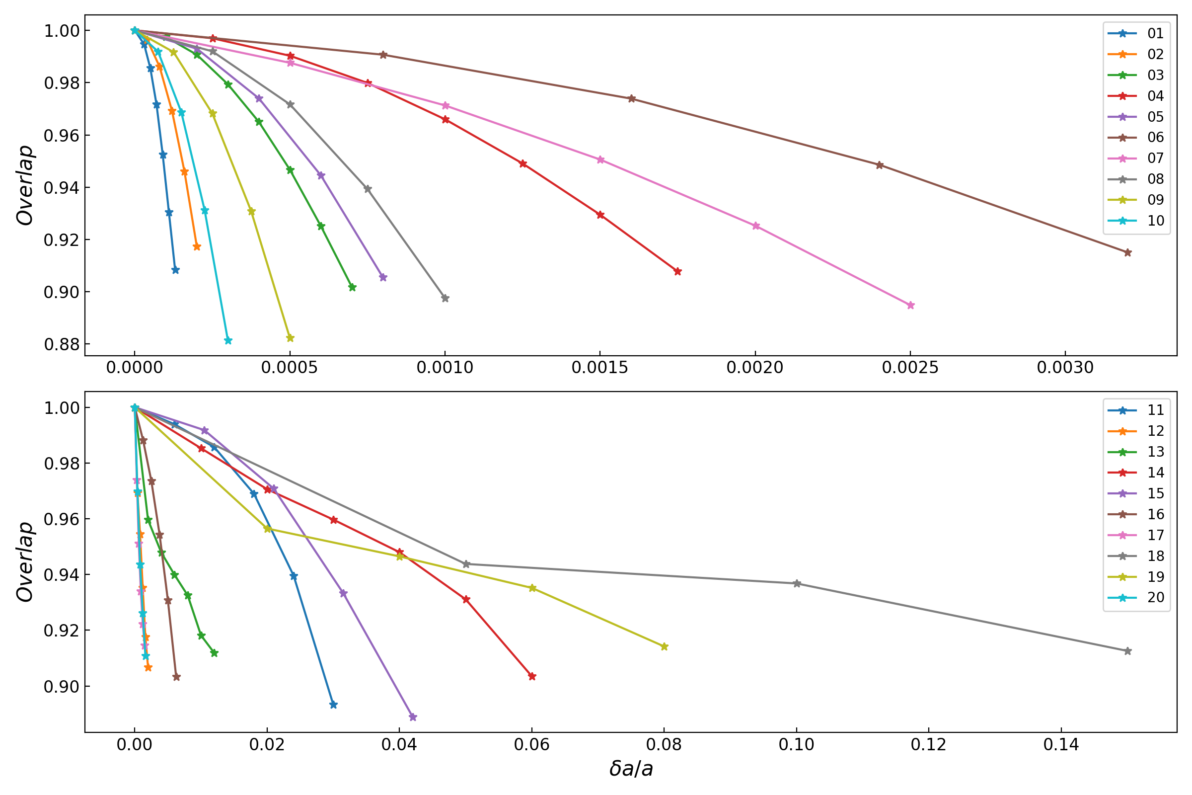
Figure 1: Overlaps between the original waveforms and the waveforms changed with spin $a$. The other parameters ($M$, $\delta_{1}$, $\delta_{2}$, $e$, $p$, $\iota$) of systems listed in Table 1 remain unchanged. The top plane represents $a$-overlap curves from the top 10 systems (X-MRI 01 to X-MRI 10). The bottom plane represents $a$-overlap curves from the last 10 systems(X-MRI 11 to X-MRI 20).

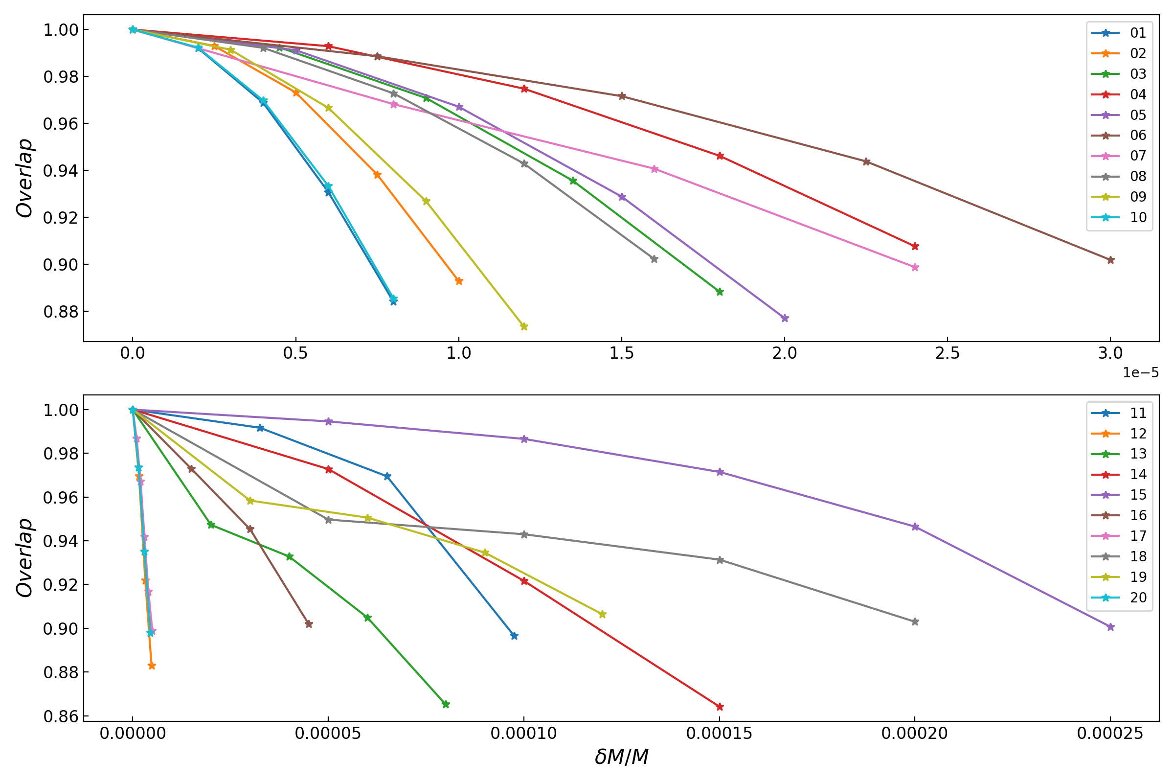
Figure 2: Overlaps between the original waveforms and the waveforms changed with mass $M$. The other parameters ($a$, $\delta_{1}$, $\delta_{2}$, $e$, $p$, $\iota$) of systems listed in Table 1 remain unchanged. The top plane represents $M$-overlap curves from the top 10 systems(X-MRI 01 to X-MRI 10). The bottom plane represents $M$-overlap curves from the last 10 systems(X-MRI 11 to X-MRI 20).

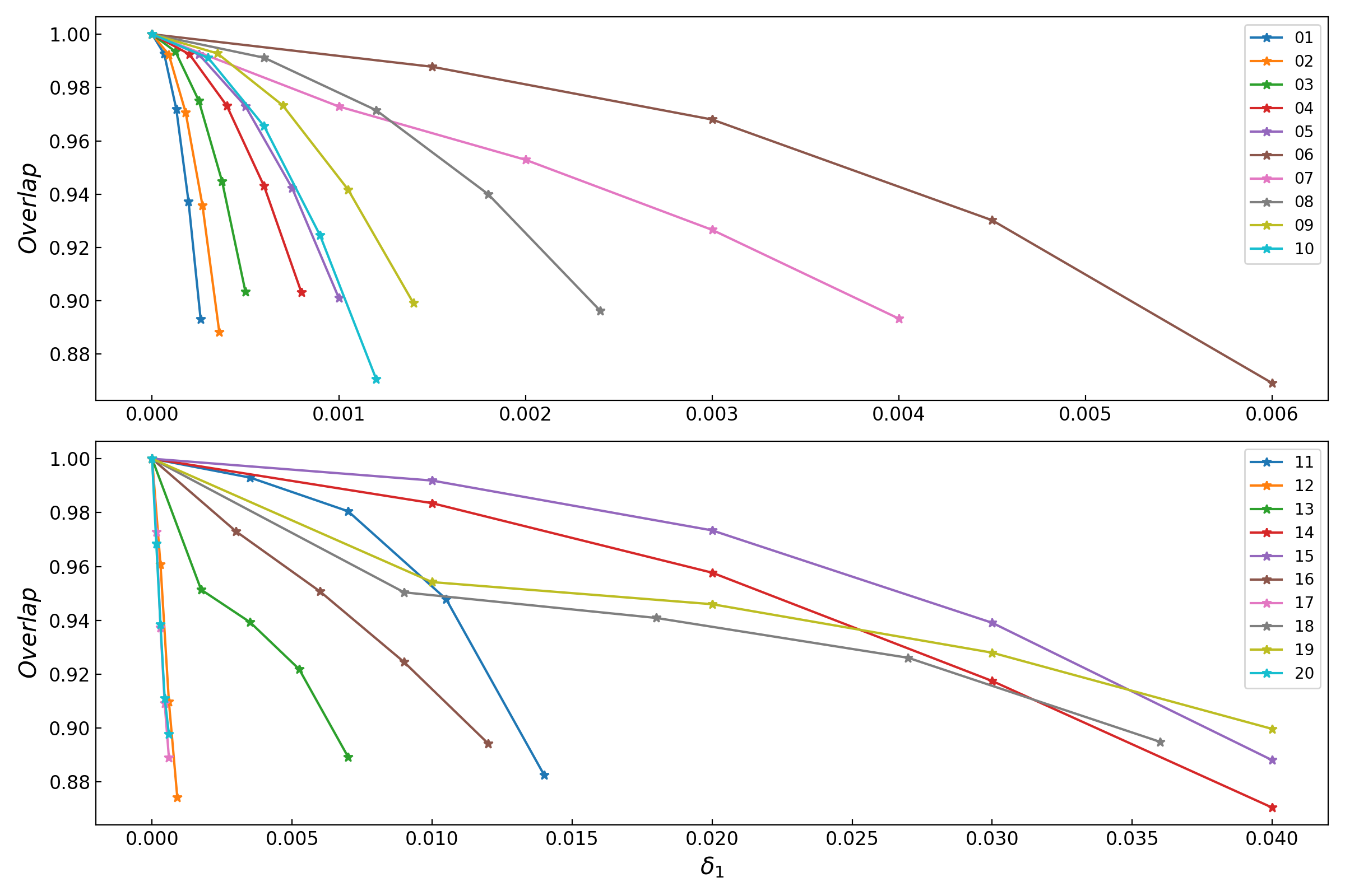
Figure 3: Overlaps between the original waveforms and the waveforms changed with deformation parameter $\delta_{1}$. The other parameters ($M$, $a$, $\delta_{2}$, $e$, $p$, $\iota$) of systems listed in Table 1 remain unchanged. The top plane represents $\delta_{1}$-overlap curves from the top 10 systems(X-MRI 01 to X-MRI 10). The bottom plane represents $\delta_{1}$-overlap curves from the last 10 systems(X-MRI 11 to X-MRI 20).

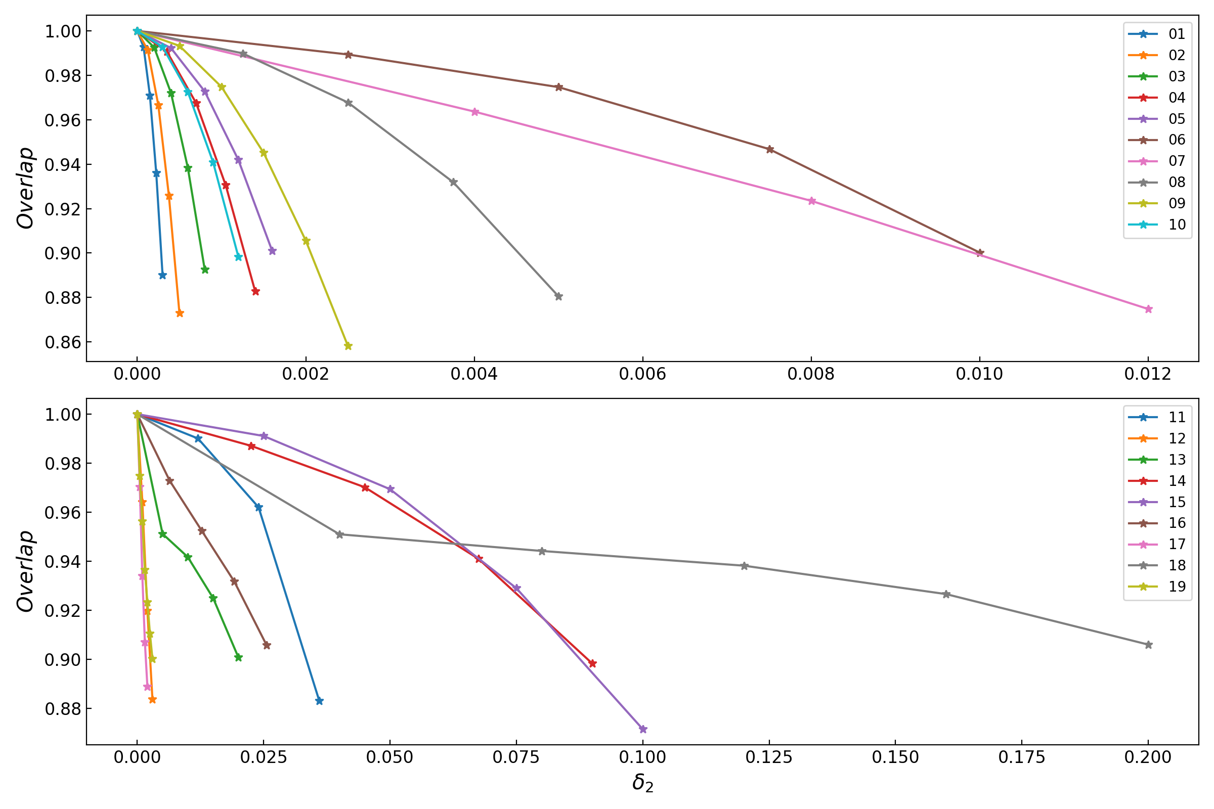
Figure 4: Overlaps between the original waveforms and the waveforms changed with deformation parameter $\delta_{2}$. The other parameters ($M$, $a$, $\delta_{1}$, $e$, $p$, $\iota$) of systems listed in Table 1 remain unchanged. The top plane represents $\delta_{2}$-overlap curves from the top 10 systems(X-MRI 01 to X-MRI 10). The bottom plane represents $\delta_{2}$-overlap curves from the last 10 systems(X-MRI 11 to X-MRI 20).

Suppose the GW signal and corresponding GW template overlaps are above 0.97Glampedakis and Babak (2006). In that case, we would find neither the deviations from GR nor the unusual parameters of X-MRIs, which is called the confusion problemGlampedakis and Babak (2006). The confusion problem can prevent us from getting accurate parameter estimation of the X-MRIs. To make sure there is no confusion in our study, we calculate the overlaps between different gravitational waveforms of twenty X-MRIs with varying parameters $\lambda_{i}$ $(\lambda_{i}=a,M,\delta_{1},\delta_{2},e,p,\iota)$. Here $(a,M)$ are the parameters of the Sgr A*, $(\delta_{1},\delta_{2})$ are the deformation parameters of the space-time from the Kerr solution, and $(e,p,\iota)$ are the parameters of orbit (eccentricity, semi-latus rectum, inclination).

Because $a,M,\delta_{1}$, and $\delta_{2}$ are the intrinsic parameters of Sgr A* and present the nature of MBH directly, we pay more attention to these four parameters. The Figs. 1-4 display the overlaps between the original waveforms and the waveforms with varying parameters $a,M,\delta_{1}$ and $\delta_{2}$. As these figures show, the overlap tends to decrease while the increment of $\lambda$ increases.

Taking the overlap value 0.97 as a criterion would give the constraints on $\lambda$. Specifically, to get the constraints on $\delta\lambda_{i}$ by the GWs of X-MRI, we first keep the other parameters fixed and generate several waveforms with varying $\lambda_{i}$. Then we calculate the overlaps between the original waveform and the waveforms with varying $\lambda_{i}$. Finally, the corresponding value of $\lambda_{i}$ when overlap equals 0.97 can be regarded as the limit of $\lambda_{i}$. From these figures, we observe the parameter constraint ability for different X-MRI varies.

4.2 Evaluate the accuracy of parameter estimation for X-MRIs

The SNRs of the X-MRI GW signals is high enough to apply the Fisher information matrix to estimate the accuracy of parameter estimation. We present the accuracy of parameter estimation for Sgr A* in this part using the Fisher information matrix. To better estimate the distance between Sgr A* and the solar system, we take account of the external parameter $R_{p}$ and constrain it by the gravitational waveforms of the X-MRIs in Table 1.

The Fisher information matrix $\Gamma$ for a GW signal $h$ parameterized by $\lambda$ is given by (See RefCutler and Flanagan (1994) for details)

$$\Gamma_{i,j}=<\frac{\partial h}{\partial\lambda_{i}}|\frac{\partial h}{\partial\lambda_{j}}>,$$ (63)

where $\lambda_{i}=(a,M,\delta_{1},\delta_{2},e,p,\iota,R_{p})$ is one of the parameters of the X-MRI system. The parameter estimation uncertainty $\Delta\lambda$ due to Gaussian noise has the normal distribution $\mathcal{N}(0,\Gamma^{-1})$ in the case of high SNR, so the root-mean-square uncertainty in the general case can be approximated as

$$\Delta\lambda_{i}=\sqrt{(\Gamma^{-1})_{i,i}}.$$ (64)

For parameter estimation uncertainty $\Delta\lambda_{i},\Delta\lambda_{j}(i\neq j)$, the corresponding likelihood is Cutler and Flanagan (1994); Babak et al. (2017); Han and Chen (2019).

$$\mathcal{L}(\lambda)\propto e^{-\frac{1}{2}\Gamma_{i,j}\Delta\lambda_{i}\Delta\lambda_{j}}.$$ (65)

For an X-MRI with eight parameters, we can get a Fisher matrix $(\Gamma_{i,j})_{8\times 8}$ by applying the results of these parameters’ preliminary constraints to equation (63). Element $\Gamma_{i,j}$ ($i\neq j$) in the Fisher matrix is the result of the combination of parameter $\lambda_{i}$ and parameter $\lambda_{j}$. With the Fisher matrix, absolute uncertainty $\Delta\lambda_{i}$ of any parameter $\lambda_{i}$ can be estimated by calculating the equation (64). Here we focus on the estimations of Sgr A*’s parameters $(a,M,\delta_{1},\delta_{2},R_{p})$.

By using the Fisher matrix, the parameter estimation accuracy of $(a,M,\delta_{1},\delta_{2},R_{p})$ for the twenty X-MRI signals is shown in Table 1. Different X-MRI systems have different abilities to estimate the uncertainty accuracy of the same parameter. For the spin of Sgr A*, the relative uncertainty $\Delta a/a$ estimated by X-MRI 01, X-MRI 02, X-MRI 03, and X-MRI 10 reach a very high precision $\sim 10^{-6}$. While $\Delta a/a$ estimated by X-MRI 15 is only $\sim 10^{-2}$. For the mass of Sgr A*, its relative uncertainty $\Delta M/M$ estimated by X-MRI 01, X-MRI 02, X-MRI 12, and X-MRI 20 reach $\sim 10^{-7}$, and $\Delta M/M$ estimated by X-MRI 15 is $\sim 10^{-4}$. For the space-time deformation around Sgr A*, $\Delta\delta_{1}$ and $\Delta\delta_{2}$ estimated by X-MRI 01 reach $\sim 10^{-6}$, while the relative uncertainty of these deformation parameters estimated by X-MRI 15 is only $\sim 10^{-2}$. For the distance $R_{p}$, its relative uncertainty $\Delta R_{p}/R_{p}$ estimated by X-MRI 01 reaches $\sim 10^{-4}$, while the accuracy of $\Delta R_{p}/R_{p}$ estimated by X-MRI 06, X-MRI 07, X-MRI 11, and X-MRI 19 is only $\sim 10^{-2}$. From the above analysis, we find that X-MRI 01 has stringent constraints for the five parameters $(a,M,\delta_{1},\delta_{2},R_{p})$. Therefore, we take X-MRI 01 as an example to present its likelihoods calculated by Eqs. 63-65. As shown in Figs. 5-7, it is obvious that the parameter estimation for X-MRI 01 may be affected by any other parameter. Thus, it is reasonable to consider the parameters of one X-MRI signal to estimate any parameter.

We further study the influence of the combination of GW signals on the parameter estimation accuracy. Here we take parameter $\alpha$ as an example to present the data processing. Firstly, we assume that there are $n$ X-MRI systems at the GC. Then, we calculate the Fisher matrices of all these signals to determine the diagonal element $\Gamma_{\alpha,\alpha}$. Sort the value of $\Gamma_{\alpha,\alpha}$ by the order of size, and the corresponding matrix will be $\Gamma_{\alpha 1},\Gamma_{\alpha 2},...,\Gamma_{\alpha n}$. Then we add these matrices to get the matrix $\Gamma_{\alpha}$,

$$\Gamma_{\alpha}=\Gamma_{\alpha 1}+\Gamma_{\alpha 2}+...+\Gamma_{\alpha n},$$ (66)

with $\Gamma_{\alpha}$, we get the estimation of absolute uncertainty from the equation

$$\Delta\alpha=\sqrt{(\Gamma_{\alpha})_{\alpha,\alpha}^{-1}}.$$ (67)

We repeat the steps of the estimation for $\Delta\alpha$, and calculate the absolute uncertainty of $a,M,\delta_{1},\delta_{2},R_{p}$. Then we will get the relative uncertainty. The results are shown in Figs. 8. The accuracy gets better as the number of X-MRI increases. With all twenty X-MRI systems in Table 1, the estimation accuracy for these parameters all reach higher precision. $\Delta a/a$ reaches the accuracy $\sim 10^{-7}$. $\Delta M/M$ reaches the accuracy $\sim 10^{-8}$. $\Delta\delta_{1}$ reaches the accuracy $\sim 10^{-6}$. $\Delta\delta_{2}$ reaches the accuracy $\sim 10^{-6}$. $\Delta R_{p}/R_{p}$ reaches the accuracy $\sim 10^{-4}$. The observation number of X-MRI systems does make sense for parameter estimation. Finally, we must emphasize that the parameter estimation results predicted by the Fisher information matrix here only stand for the ideal situation, in the actual parameter estimation practice, because of all kinds of noise, the results would not be that kind of good.

$\Delta a/a$	$\Delta M/M$	$\Delta\delta_{1}$	$\Delta\delta_{2}$	$\Delta R_{p}/R_{p}$
$5.38\times 10^{-7}$	$7.02\times 10^{-8}$	$2.40\times 10^{-6}$	$2.18\times 10^{-6}$	$6.05\times 10^{-4}$

Table 2: Results of parameter estimation accuracy of all the 20 X-MRI systems.

5 Conclusions and Outlook

Sgr A* is the closest MBH for the Solar system. It is therefore an ideal laboratory to study the properties of black holes and to test alternative theories of gravity. To investigate the structure of Sgr A*, we simulate the GW signals for twenty X-MRI systems using the KRZ metric and the kludge waveform. We then apply the Fisher information matrix method to these GW signals. With a single GW X-MRI event detected, we were able to obtain a relatively accurate estimate of spin $a$, mass $M$, and deviation parameters $\delta_{1},\delta_{2}$. More X-MRI observations would improve the measurement of the above parameters.

In practice, galactic binaries(GBs) and EMRIs are also promising sources of space-borne GW detectors like LISAAmaro-Seoane et al. (2017). GBs, comprise primarily white dwarfs but also neutron stars and stellar-origin black holes, emit continuous and nearly monochromatic GW signals. X-MRIs can be also regarded as monochromatic sources for space-borne detectors, while the signals of X-MRIs could reach high SNRs, making X-MRIs feasible to be distinguished from weaker sources such as GBsAmaro-Seoane (2019). On the contrary, EMRIs, which evolve relatively rapidly, are polychromatic sourcesAmaro-Seoane (2019). Therefore, EMRIs and X-MRIs could be complementary in studying the space-time of MBH.

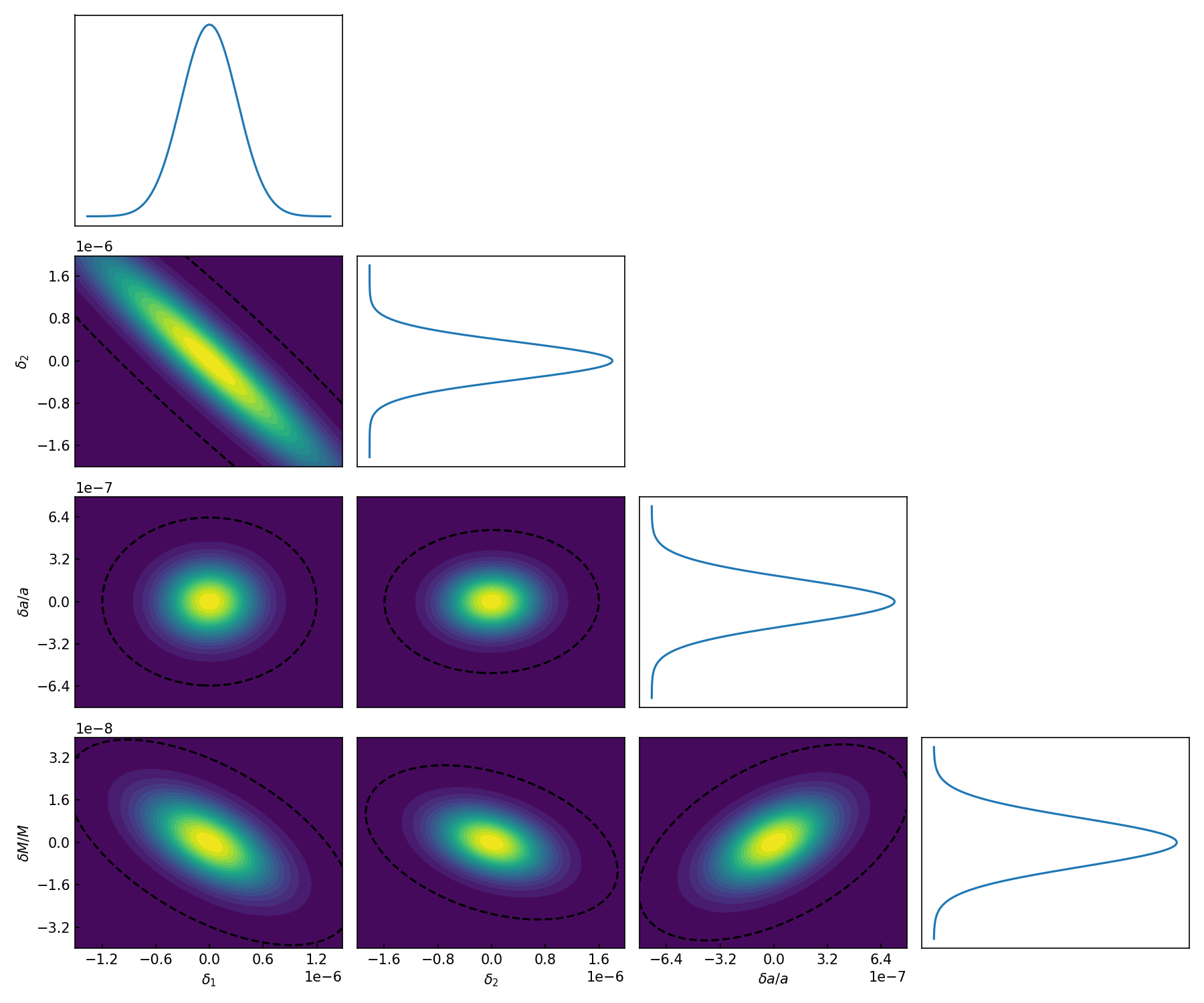
Figure 5: Likelihoods of $(\delta_{1},\delta M/M)$, $(\delta_{1},\delta a/a)$, $(\delta_{1},\delta_{2})$, $(\delta_{2},\delta M/M)$, $(\delta_{2},\delta a/a)$, $(\delta a/a,\delta M/M)$ derived from the Fisher matrix of X-MRI 01. The black dashed eclipses show the $3\sigma$ confidence level. The upper and the four right-hand panels show the marginalized probability distribution for $\delta_{1},\delta_{2},\delta a/a$ and $\delta M/M$, respectively.

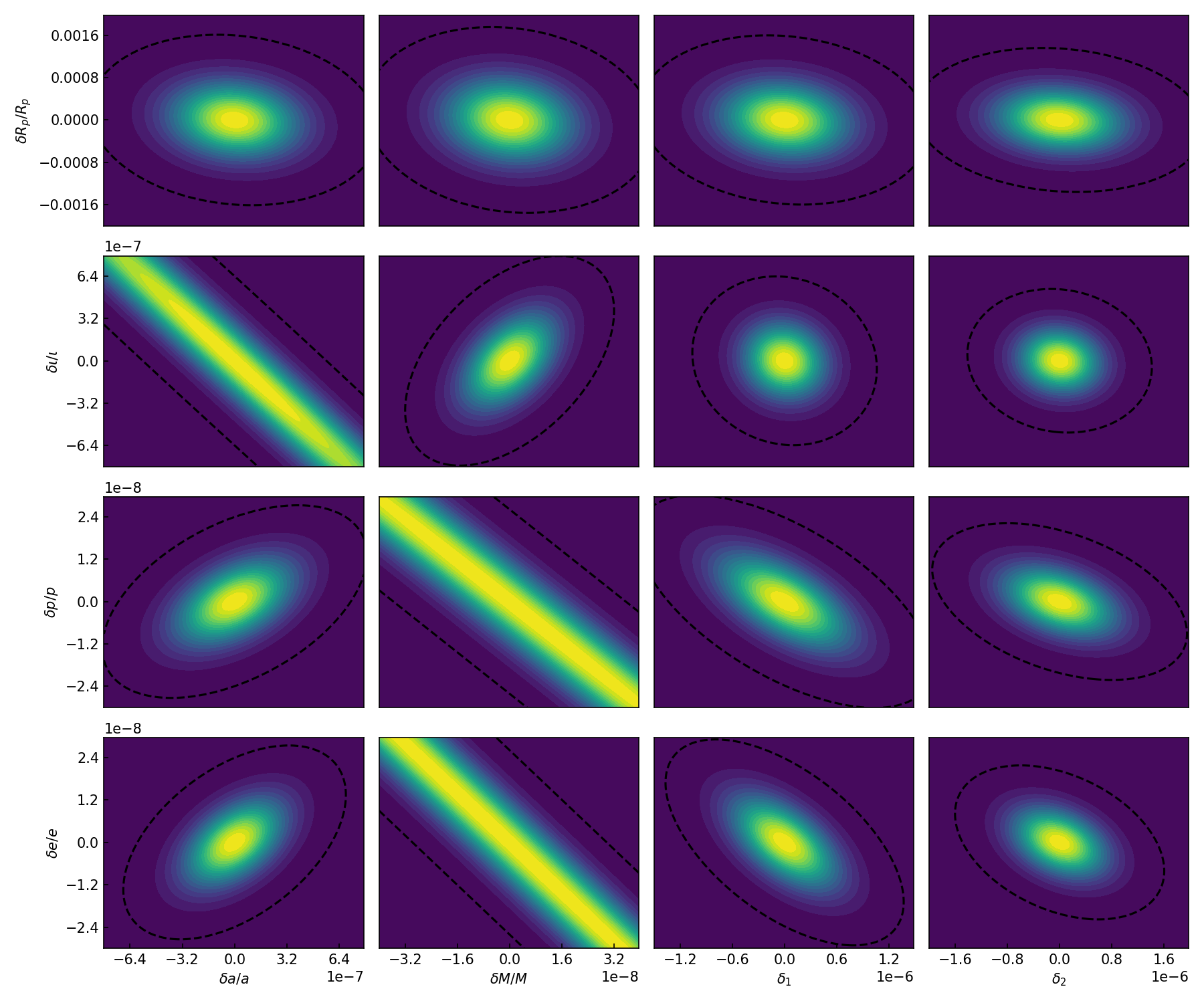
Figure 6: Likelihoods of $(\delta a/a,\delta e/e)$, $(\delta a/a,\delta p/p)$, $(\delta a/a,\delta\iota/\iota)$, $(\delta a/a,\delta R_{p}/R_{p})$, $(\delta M/M,\delta e/e)$, $(\delta M/M,\delta p/p)$, $(\delta M/M,\delta\iota/\iota)$, $(\delta M/M,\delta R_{p}/R_{p})$, $(\delta_{1},\delta e/e)$, $(\delta_{1},\delta p/p)$, $(\delta_{1},\delta\iota/\iota)$, $(\delta_{1},\delta R_{p}/R_{p})$, $(\delta_{2},\delta e/e)$, $(\delta_{2},\delta p/p)$, $(\delta_{2},\delta\iota/\iota)$, $(\delta_{2},\delta R_{p}/R_{p})$ derived from the Fisher matrix of X-MRI 01. The black dashed eclipses show the $3\sigma$ confidence level.

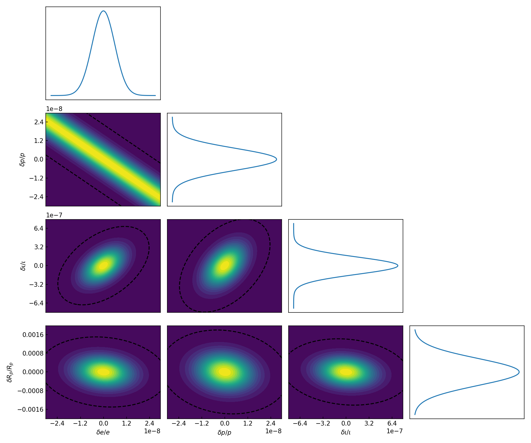
Figure 7: Likelihoods of $(\delta e/e,\delta R_{p}/R_{p})$, $(\delta e/e,\delta\iota/\iota)$, $(\delta e/e,\delta p/p)$, $(\delta p/p,\delta R_{p}/R_{p})$, $(\delta p/p,\delta\iota/\iota)$, $(\delta\iota/\iota,\delta R_{p}/R_{p})$ derived from the Fisher matrix of X-MRI 01. The black dashed eclipses show the $3\sigma$ confidence level. The upper and the four right-hand panels show the marginalized probability distribution for $\delta e/e,\delta p/p,\delta\iota/\iota$ and $\delta R_{p}/R_{p}$, respectively.

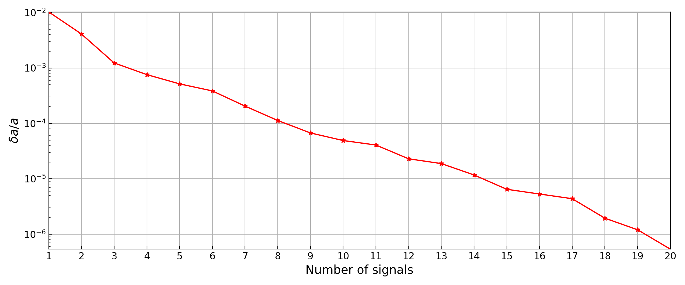
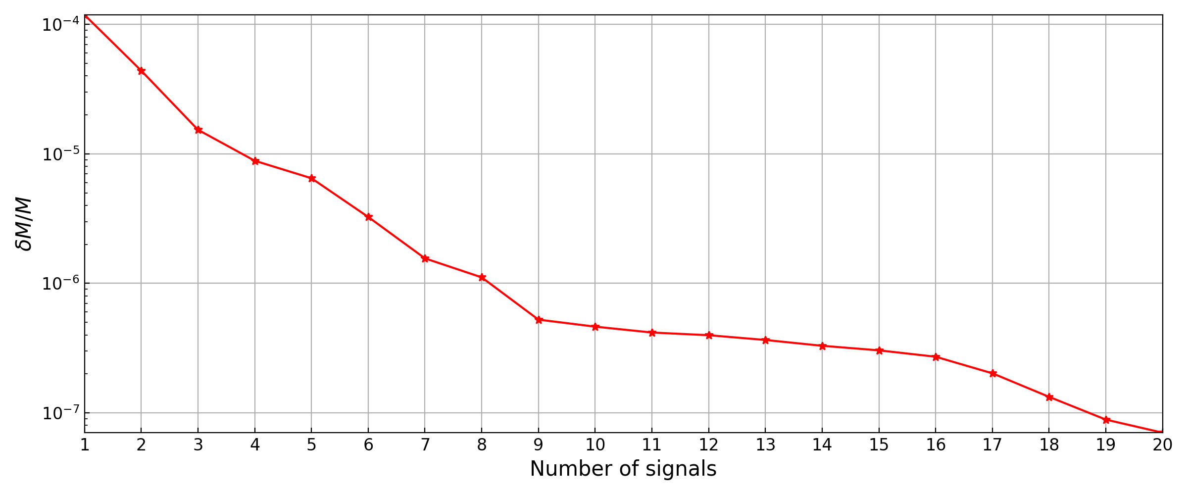
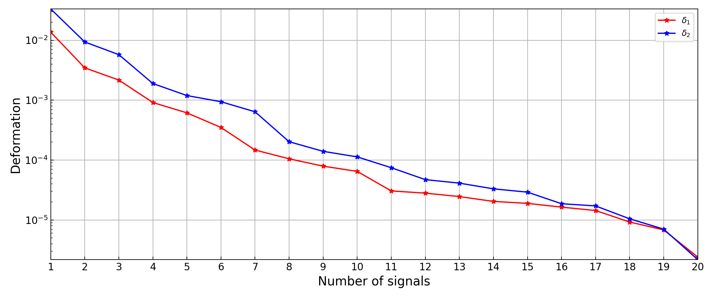
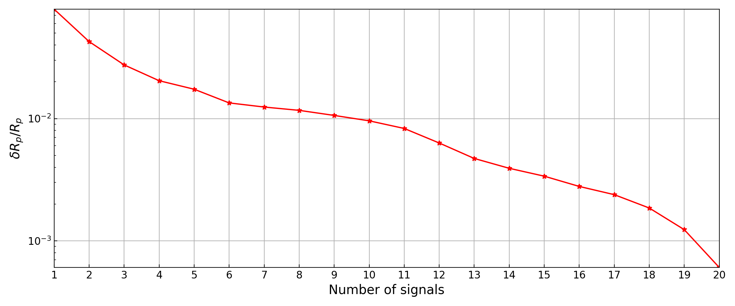
Figure 8: The relation between the parameter estimation accuracy and the X-MRI signals number. The parameter in the first plane is $\delta a/a$, in the second plane is $\delta M/M$, in the third plane are $\delta_{1}$(red) and $\delta_{2}$(blue), in the fourth plane is $\delta R_{p}/R_{p}$.

conceptualization, Shu-Cheng Yang; methodology, Huijiao Luo, Yuan-Hao Zhang, Chen Zhang and Shu-Cheng Yang; software, Huijiao Luo, Yuan-Hao Zhang and Shu-Cheng Yang; validation, Shu-Cheng Yang; formal analysis, Huijiao Luo, Yuan-Hao Zhang and Shu-Cheng Yang; investigation, Huijiao Luo, Yuan-Hao Zhang Chen Zhang, and Shu-Cheng Yang; resources, Shu-Cheng Yang; data curation, Huijiao Luo, Yuan-Hao Zhang and Shu-Cheng Yang; writing–original draft preparation, Huijiao Luo; writing–review and editing, Shu-Cheng Yang and Yuan-Hao Zhang; visualization, Huijiao Luo ; supervision, Shu-Cheng Yang; project administration, Shu-Cheng Yang; funding acquisition, Shu-Cheng Yang. All authors have read and agreed to the published version of the manuscript.

This work is supported by The National Key R&D Program of China (Grant No. 2021YFC2203002), NSFC (National Natural Science Foundation of China) No. 11773059 and No. 12173071.

References

- B.P. Abbott et al. (2016) (The LIGO Scientific Collaboration and the Virgo Collaboration) B.P. Abbott et al. (The LIGO Scientific Collaboration and the Virgo Collaboration). Observation of gravitational waves from a binary black hole merger. Phys. Rev. Lett. 2016, 116, 061102.
- B.P. Abbott et al. (2017) (The LIGO Scientific Collaboration and the Virgo Collaboration) B.P. Abbott et al. (The LIGO Scientific Collaboration and the Virgo Collaboration). GW170817: observation of gravitational waves from a binary neutron star inspiral. Phys. Rev. Lett. 2017, 119, 161101.
- B.P. Abbott et al. (2019) (The LIGO Scientific Collaboration and the Virgo Collaboration) B.P. Abbott et al. (The LIGO Scientific Collaboration and the Virgo Collaboration). GWTC-1: a gravitational-wave transient catalog of compact binary mergers observed by LIGO and Virgo during the first and second observing runs. Phys. Rev. X 2019, 9, 031040.
- R. Abbott et al. (2021) (The LIGO Scientific Collaboration and the Virgo Collaboration) R. Abbott et al. (The LIGO Scientific Collaboration and the Virgo Collaboration). GWTC-2: compact binary coalescences observed by LIGO and Virgo during the first half of the third observing run. Phys. Rev. X 2021, 11, 021053.
- R. Abbott et al. (2021) (The LIGO Scientific Collaboration, the Virgo Collaboration, and the KAGRA Collaboration) R. Abbott et al. (The LIGO Scientific Collaboration, the Virgo Collaboration, and the KAGRA Collaboration). GWTC-3: Compact Binary Coalescences Observed by LIGO and Virgo During the Second Part of the Third Observing Run, 2021, [arXiv:gr-qc/2111.03606].
- J. Aasi et al. (2015) (The LIGO Scientific Collaboration) J. Aasi et al. (The LIGO Scientific Collaboration). Advanced LIGO. Class. Quant. Grav. 2015, 32, 074001.
- Acernese et al. (2014) Acernese, F.a.; Agathos, M.; Agatsuma, K.; Aisa, D.; Allemandou, N.; Allocca, A.; Amarni, J.; Astone, P.; Balestri, G.; Ballardin, G.; et al. Advanced Virgo: a second-generation interferometric gravitational wave detector. Class. Quant. Grav. 2014, 32, 024001.
- The KAGRA Collaboration (2019) The KAGRA Collaboration. KAGRA: 2.5 generation interferometric gravitational wave detector. Nature Astronomy 2019, 3, 35–40.
- Amaro-Seoane et al. (2007) Amaro-Seoane, P.; Gair, J.R.; Freitag, M.; Miller, M.C.; Mandel, I.; Cutler, C.J.; Babak, S. Intermediate and extreme mass-ratio inspirals—astrophysics, science applications and detection using LISA. Classical and Quantum Gravity 2007, 24, R113.
- Amaro-Seoane et al. (2017) Amaro-Seoane, P.; Audley, H.; Babak, S.; Baker, J.; Barausse, E.; Bender, P.; Berti, E.; Binetruy, P.; Born, M.; Bortoluzzi, D.; et al. Laser Interferometer Space Antenna, 2017, [arXiv:gr-qc/1702.00786].
- Hu and Wu (2017) Hu, W.R.; Wu, Y.L. The Taiji Program in Space for gravitational wave physics and the nature of gravity. Natl. Sci. Rev. 2017, 4, 685.
- Luo et al. (2016) Luo, J.; Chen, L.S.; Duan, H.Z.; Gong, Y.G.; Hu, S.; Ji, J.; Liu, Q.; Mei, J.; Milyukov, V.; Sazhin, M.; et al. TianQin: a space-borne gravitational wave detector. Class. Quantum Gravity 2016, 33, 035010.
- Gair et al. (2010) Gair, J.R.; Tang, C.; Volonteri, M. LISA extreme-mass-ratio inspiral events as probes of the black hole mass function. Phys. Rev. D 2010, 81, 104014.
- Chua et al. (2017) Chua, A.J.; Moore, C.J.; Gair, J.R. Augmented kludge waveforms for detecting extreme-mass-ratio inspirals. Phys. Rev. D 2017, 96, 044005.
- Gourgoulhon et al. (2019) Gourgoulhon, E.; Le Tiec, A.; Vincent, F.H.; Warburton, N. Gravitational waves from bodies orbiting the Galactic Center black hole and their detectability by LISA. Astron. Astrophys 2019, 627, A92.
- Amaro-Seoane (2019) Amaro-Seoane, P. Extremely large mass-ratio inspirals. Phys. Rev. D 2019, 99, 123025.
- Burrows and Liebert (1993) Burrows, A.; Liebert, J. The science of brown dwarfs. Rev. Mod. Phys. 1993, 65, 301.
- Freitag (2002) Freitag, M. Gravitational waves from stars orbiting the Sagittarius A* black hole. ApJ 2002, 583, L21.
- Eckart and Genzel (1996) Eckart, A.; Genzel, R. Observations of stellar proper motions near the Galactic Centre. Nature 1996, 383, 415–417.
- Ghez et al. (1998) Ghez, A.M.; Klein, B.; Morris, M.; Becklin, E. High proper-motion stars in the vicinity of Sagittarius A*: Evidence for a supermassive black hole at the center of our galaxy. ApJ 1998, 509, 678.
- Ghez et al. (2008) Ghez, A.M.; Salim, S.; Weinberg, N.; Lu, J.; Do, T.; Dunn, J.; Matthews, K.; Morris, M.; Yelda, S.; Becklin, E.; et al. Measuring distance and properties of the Milky Way’s central supermassive black hole with stellar orbits. ApJ 2008, 689, 1044.
- Genzel et al. (2010) Genzel, R.; Eisenhauer, F.; Gillessen, S. The Galactic Center massive black hole and nuclear star cluster. Rev. Mod. Phys. 2010, 82, 3121.
- Afrin et al. (2021) Afrin, M.; Kumar, R.; Ghosh, S.G. Parameter estimation of hairy Kerr black holes from its shadow and constraints from M87. MNRAS 2021, 504, 5927–5940.
- Konoplya et al. (2016) Konoplya, R.; Rezzolla, L.; Zhidenko, A. General parametrization of axisymmetric black holes in metric theories of gravity. Phys. Rev. D 2016, 93, 064015.
- R. Abbott et al. (2021) (The LIGO Scientific Collaboration, the Virgo Collaboration, and the KAGRA Collaboration) R. Abbott et al. (The LIGO Scientific Collaboration, the Virgo Collaboration, and the KAGRA Collaboration). Tests of General Relativity with GWTC-3 2021. [arXiv:gr-qc/2112.06861].
- Hu et al. (2022) Hu, S.; Deng, C.; Li, D.; Wu, X.; Liang, E. Observational signatures of Schwarzschild-MOG black holes in scalar-tensor-vector gravity: shadows and rings with different accretions. Eur. Phys. J. C 2022, 82, 1–17.
- Cao et al. (2022) Cao, W.; Liu, W.; Wu, X. Integrability of Kerr-Newman spacetime with cloud strings, quintessence and electromagnetic field. Phys. Rev. D 2022, 105, 124039.
- Zhang et al. (2022) Zhang, H.; Zhou, N.; Liu, W.; Wu, X. Equivalence between two charged black holes in dynamics of orbits outside the event horizons. Gen. Relat. Gravit. 2022, 54, 1–22.
- Yang et al. (2022) Yang, D.; Cao, W.; Zhou, N.; Zhang, H.; Liu, W.; Wu, X. Chaos in a Magnetized Modified Gravity Schwarzschild Spacetime. Universe 2022, 8, 320.
- Zhang et al. (2021) Zhang, H.; Zhou, N.; Liu, W.; Wu, X. Charged particle motions near non-Schwarzschild black holes with external magnetic fields in modified theories of gravity. Universe 2021, 7, 488.
- Yi and Wu (2020) Yi, M.; Wu, X. Dynamics of charged particles around a magnetically deformed Schwarzschild black hole. Phys. Scr. 2020, 95, 085008.
- Johannsen and Psaltis (2011) Johannsen, T.; Psaltis, D. Metric for rapidly spinning black holes suitable for strong-field tests of the no-hair theorem. Phys. Rev. D 2011, 83, 124015.
- Ni et al. (2016) Ni, Y.; Jiang, J.; Bambi, C. Testing the Kerr metric with the iron line and the KRZ parametrization. J. Cosmol. Astropart. Phys 2016, 2016, 014.
- Drake and Szekeres (2000) Drake, S.P.; Szekeres, P. Uniqueness of the Newman–Janis algorithm in generating the Kerr–Newman metric. Gen. Relativ. Gravit 2000, 32, 445–457.
- Jiang et al. (2015) Jiang, J.; Bambi, C.; Steiner, J.F. Using iron line reverberation and spectroscopy to distinguish Kerr and non-Kerr black holes. JCAP 2015, 2015, 025.
- Horne and Horowitz (1992) Horne, J.H.; Horowitz, G.T. Rotating dilaton black holes. Phys. Rev. D 1992, 46, 1340.
- Cardoso et al. (2014) Cardoso, V.; Pani, P.; Rico, J. On generic parametrizations of spinning black-hole geometries. Phys. Rev. D 2014, 89, 064007.
- Younsi et al. (2016) Younsi, Z.; Zhidenko, A.; Rezzolla, L.; Konoplya, R.; Mizuno, Y. New method for shadow calculations: Application to parametrized axisymmetric black holes. Phys. Rev. D 2016, 94, 084025.
- Zhou et al. (2022) Zhou, N.; Zhang, H.; Liu, W.; Wu, X. A Note on the Construction of Explicit Symplectic Integrators for Schwarzschild Spacetimes. ApJ 2022, 927, 160.
- Wang et al. (2021a) Wang, Y.; Sun, W.; Liu, F.; Wu, X. Construction of Explicit Symplectic Integrators in General Relativity. I. Schwarzschild Black Holes. ApJ 2021, 907, 66.
- Wang et al. (2021b) Wang, Y.; Sun, W.; Liu, F.; Wu, X. Construction of Explicit Symplectic Integrators in General Relativity. II. Reissner–Nordström Black Holes. ApJ 2021, 909, 22.
- Wang et al. (2021c) Wang, Y.; Sun, W.; Liu, F.; Wu, X. Construction of Explicit Symplectic Integrators in General Relativity. III. Reissner–Nordström-(anti)-de Sitter Black Holes. ApJS 2021, 254, 8.
- Wu et al. (2021) Wu, X.; Wang, Y.; Sun, W.; Liu, F. Construction of explicit symplectic integrators in general relativity. IV. Kerr black holes. ApJ 2021, 914, 63.
- Sun et al. (2021) Sun, W.; Wang, Y.; Liu, F.; Wu, X. Applying explicit symplectic integrator to study chaos of charged particles around magnetized Kerr black hole. Eur. Phys. J. C 2021, 81, 1–10.
- Xin et al. (2019) Xin, S.; Han, W.B.; Yang, S.C. Gravitational waves from extreme-mass-ratio inspirals using general parametrized metrics. Phys. Rev. D 2019, 100, 084055.
- Hughes (2001) Hughes, S.A. Evolution of circular, nonequatorial orbits of Kerr black holes due to gravitational-wave emission. II. Inspiral trajectories and gravitational waveforms. Phys. Rev. D 2001, 64, 064004.
- Barack and Cutler (2004) Barack, L.; Cutler, C. LISA capture sources: Approximate waveforms, signal-to-noise ratios, and parameter estimation accuracy. Phys. Rev. D 2004, 69, 082005.
- Drasco and Hughes (2006) Drasco, S.; Hughes, S.A. Gravitational wave snapshots of generic extreme mass ratio inspirals. Phys. Rev. D 2006, 73, 024027.
- Babak et al. (2007) Babak, S.; Fang, H.; Gair, J.R.; Glampedakis, K.; Hughes, S.A. “Kludge” gravitational waveforms for a test-body orbiting a Kerr black hole. Phys. Rev. D 2007, 75, 024005.
- Chua and Gair (2015) Chua, A.J.; Gair, J.R. Improved analytic extreme-mass-ratio inspiral model for scoping out eLISA data analysis. Class. Quant. Grav. 2015, 32, 232002.
- Rüdiger (1981) Rüdiger, R. Conserved quantities of spinning test particles in general relativity. I. Proceedings of the Royal Society of London. A. Mathematical and Physical Sciences 1981, 375, 185–193.
- Rüdiger (1983) Rüdiger, R. Conserved quantities of spinning test particles in general relativity. II. Proceedings of the Royal Society of London. A. Mathematical and Physical Sciences 1983, 385, 229–239.
- Wang et al. (2016) Wang, S.C.; Wu, X.; Liu, F.Y. Implementation of the velocity scaling method for elliptic restricted three-body problems. MNRAS 2016, 463, 1352–1362.
- Wang et al. (2018) Wang, S.; Huang, G.; Wu, X. Simulations of dissipative circular restricted three-body problems using the velocity-scaling correction method. ApJ 2018, 155, 67.
- Deng et al. (2020) Deng, C.; Wu, X.; Liang, E. The use of Kepler solver in numerical integrations of quasi-Keplerian orbits. MNRAS 2020, 496, 2946–2961.
- Li and Wu (2017) Li, D.; Wu, X. Modification of logarithmic Hamiltonians and application of explicit symplectic-like integrators. MNRAS 2017, 469, 3031–3041.
- Luo et al. (2017) Luo, J.; Wu, X.; Huang, G.; Liu, F. Explicit symplectic-like integrators with midpoint permutations for spinning compact binaries. ApJ 2017, 834, 64.
- Pan et al. (2021) Pan, G.; Wu, X.; Liang, E. Extended phase-space symplectic-like integrators for coherent post-Newtonian Euler-Lagrange equations. Phys. Rev. D 2021, 104, 044055.
- Liu et al. (2016) Liu, L.; Wu, X.; Huang, G.; Liu, F. Higher order explicit symmetric integrators for inseparable forms of coordinates and momenta. MNRAS 2016, 459, 1968–1976.
- Mei et al. (2013a) Mei, L.; Wu, X.; Liu, F. On preference of Yoshida construction over Forest–Ruth fourth-order symplectic algorithm. Eur. Phys. J. C 2013, 73, 1–8.
- Mei et al. (2013b) Mei, L.; Ju, M.; Wu, X.; Liu, S. Dynamics of spin effects of compact binaries. MNRAS 2013, 435, 2246–2255.
- Zhong et al. (2010) Zhong, S.Y.; Wu, X.; Liu, S.Q.; Deng, X.F. Global symplectic structure-preserving integrators for spinning compact binaries. Phys. Rev. D 2010, 82, 124040.
- Finn (1992) Finn, L.S. Detection, measurement, and gravitational radiation. Phys. Rev. D 1992, 46, 5236.
- Chabrier and Baraffe (2000) Chabrier, G.; Baraffe, I. Theory of low-mass stars and substellar objects. Annu. Rev. Astron. Astrophys. 2000, 38, 337–377.
- Shcherbakov et al. (2012) Shcherbakov, R.V.; Penna, R.F.; McKinney, J.C. Sagittarius A* accretion flow and black hole parameters from general relativistic dynamical and polarized radiative modeling. ApJ 2012, 755, 133.
- Eisenhauer et al. (2003) Eisenhauer, F.; Schödel, R.; Genzel, R.; Ott, T.; Tecza, M.; Abuter, R.; Eckart, A.; Alexander, T. A geometric determination of the distance to the galactic center. ApJ 2003, 597, L121.
- Menten et al. (1997) Menten, K.M.; Reid, M.J.; Eckart, A.; Genzel, R. The position of Sagittarius A*: accurate alignment of the radio and infrared reference frames at the Galactic Center. ApJ 1997, 475, L111.
- Glampedakis and Babak (2006) Glampedakis, K.; Babak, S. Mapping spacetimes with LISA: inspiral of a test body in a ‘quasi-Kerr’field. Class. Quant. Grav. 2006, 23, 4167.
- Cutler and Flanagan (1994) Cutler, C.; Flanagan, E.E. Gravitational waves from merging compact binaries: How accurately can one extract the binary’s parameters from the inspiral waveform? Phys. Rev. D 1994, 49, 2658.
- Babak et al. (2017) Babak, S.; Gair, J.; Sesana, A.; Barausse, E.; Sopuerta, C.F.; Berry, C.P.; Berti, E.; Amaro-Seoane, P.; Petiteau, A.; Klein, A. Science with the space-based interferometer LISA. V. Extreme mass-ratio inspirals. Phys. Rev. D 2017, 95, 103012.
- Han and Chen (2019) Han, W.B.; Chen, X. Testing general relativity using binary extreme-mass-ratio inspirals. MNRAS 2019, 485, L29–L33.