Quantum Circuit Compiler for a Shuttling-Based Trapped-Ion Quantum Computer

Abstract

The increasing capabilities of quantum computing hardware and the challenge of realizing deep quantum circuits require fully automated and efficient tools for compiling quantum circuits. To express arbitrary circuits in a sequence of native gates specific to the quantum computer architecture, it is necessary to make algorithms portable across the landscape of quantum hardware providers. In this work, we present a compiler capable of transforming and optimizing a quantum circuit targeting a shuttling-based trapped-ion quantum processor. It consists of custom algorithms set on top of the quantum circuit framework Pytket. The performance was evaluated for a wide range of quantum circuits and the results show that the gate counts can be reduced by factors up to 5.1 compared to standard Pytket and up to 2.2 compared to standard Qiskit compilation.

1 Introduction

The current rapid maturation of quantum information processing platforms [1] brings meaningful scientific and commercial applications of quantum computing within reach. While it seems unlikely that fault-tolerant devices [2, 3] will scale to sufficiently large numbers of logical qubits in the near future, noisy intermediate scale quantum (NISQ) devices are predicted to lead the way into the era of applied quantum computing [4]. The quantum compiler stack of such platforms will crucially determine their capabilities and performance: First, fully automated, hardware-agnostic front-ends will enable access for non-expert users from various scientific disciplines and industry. Second, optimizations performed at the compilation stage will allow overcoming limitations due to noise and limited qubit register sizes, thereby increasing the functionality of a given NISQ platform.

As quantum hardware scales to larger qubit register sizes and deeper gate sequences, the platforms become increasingly complex and require tool support and automation. It is no longer feasible to manually design quantum circuits and use fixed decomposition schemes to convert the algorithm input into a complete set of qubit operations which the specific quantum hardware can execute, referred to as its native gate set. Dedicated quantum compilers are required for the optimized conversion of large circuits into low-level hardware instructions.

Fig. 1: Linear shuttling-based segmented ion trap architecture: The ions are stored in small groups at different segments of the architecture. The lasers performing the gate operations (here on the red ions) are directed only to a specific segment, the laser interaction zone (LIZ, purple segment). The following operations reconfigure the ion positions (from left to right): merging ions into a new group (green ions), physically swapping ions (blue ions), splitting a group (purple ions), and translating ions between different segments (yellow ion).

In this work, we present such a circuit compiler developed for a shuttling-based trapped-ion quantum computing platform [5, 6, 7, 8]. This platform encodes qubits in long-lived states of atomic ions stored in segmented microchip ion traps, as shown in Fig. 1. To increase potential scalability, subsets of the qubit register (a belonging set of qubits) are stored at different trap segments. Shuttling operations, performed by changing the voltages applied to the trap electrodes, dynamically reconfigure the register between subsequent gate operations. Gates are executed at specific trap sites and are driven by laser or microwave radiation. While this approach provides all-to-all connectivity within the register and avoids crosstalk errors, the shuttling operations incur substantial timing overhead, resulting in rather slow operation timescales in the order of tens of microseconds per operation [9]. This can lead to increased error rates because the reduced operation speed aggravates dephasing. Furthermore, the shuttling operations can lead to reduced gate fidelities due to shuttling-induced heating of the qubit ions. Therefore, besides compiling a given circuit into a native gate set, the main task of the gate compiler stage of a shuttling-based platform is to minimize the required amount of shuttling operations. This is achieved by minimizing the overall gate count and by arranging the execution order of the gates in a favorable way. A subsequent Shuttling Compiler stage, which is beyond the scope of this work, handles the task of generating schedules of shuttling operations based on the compilation result [10, 11, 12, 13, 14].

This paper focuses on taking into account the properties of the shuttling-based quantum computing hardware when optimizing the circuit. It provides insights into how the hardware architecture can be exploited to further improve the fidelity of the compiled circuit. Since we use many state-of-the-art transformations and algorithms as the basis for our circuit compiler, much of this work is also applicable to more general quantum circuit compilers.

The structure of this paper is as follows: Sec. 2 reviews existing circuit optimization techniques. Sec. 3 defines the representation of quantum circuits used in this work. This is followed in Sec. 4 by a detailed description of all circuit transformation algorithms used. Parameterized circuits and their compilation are discussed in Sec. 5. An evaluation of the methods is presented in Sec. 6 and shows the benefits of our circuit compiler.

2 Background

Due to the increasing size and complexity of quantum circuits, automatic circuit compilation is required to execute quantum circuits on different platforms. For this purpose, powerful frameworks for quantum computing [15, 16, 17] have been developed. Although their features vary widely, all frameworks provide some kind of built-in optimization.

While the simplest form of circuit compilation replaces gates with predefined sequences of other gates (often referred to as decomposition), more advanced techniques minimize the number of gates. A common strategy is to reduce the overall gate count, with a particular focus on expensive two-qubit gates [18, 19, 20]. One such approach uses a different circuit representation called ZX-calculus [21], which allows simplifications at the functional level. Another algorithm searches for common circuit patterns, called templates, and replaces them with shorter or otherwise preferable but functionally identical gate sequences [20].

When compiling quantum circuits, the qubit mapping is often considered as well. Ideally, each qubit can interact with any other qubit, allowing two-qubit gates to be executed between any pair of qubits. However, for existing platforms, interactions are limited to nearest neighbor topology or full connectivity within subsets of limited size. Mapping the qubits from the algorithmic circuit to physical qubits subjected to these hardware constraints is called the routing problem [15]. To make arbitrary two-qubit gates executable on the quantum hardware, SWAP gates must be inserted into the circuit [22, 23, 24, 25]. In the case of ion trap quantum computers, ion positions can be physically swapped to establish dynamic all-to-all connectivity. Consequently, no computational SWAP gates need to be inserted at this stage.

The Pytket framework [15] provides a wide variety of circuit transformation algorithms and therefore we use it as the operational basis for the custom circuit compiler described in this paper. Functionality such as the removal of redundancies and the rebasing of arbitrary gates into the native gate set is mainly realized using Pytket’s built-in functions. Since Pytket is designed for superconducting architectures, we have additionally developed and implemented some specific functionalities for trapped-ion quantum computers. These include concatenating multiple local rotations into global rotations, restricting gate parameters to a fixed set of values, and improving gate ordering.

Previous approaches to quantum circuit compilers have focused on different architectures such as photonic [26] and superconducting quantum computers [27]. These compilers share similarities with our approach, such as the use of the ZX-calculus [28] to optimize the circuits. There are also several Pytket extensions for different quantum devices [29]. However, there are inherent differences in the kind of parallelism offered by the hardware and thus should be used to get the best results. The same applies to the native operations (like the physical ion swap in our case).

3 Graph description of the quantum circuit

This section describes a quantum circuit as a directed acyclic graph (DAG), which is the data structure on which Pytket and our custom subroutines operate. The first subsection defines the DAG, and the second subsection constructs it. Such a graph is depicted in Fig. 2. At the end of this section, we describe the native gate set of our platform.

3.1 Graph definition

We consider a quantum circuit consisting of a set $\mathcal{Q}=\{q_{0},\dots,q_{n-1}\}$ of $n$ qubits. The circuit is represented as a directed acyclic graph $C=\left(\mathcal{V}\cup\mathcal{G}\cup\mathcal{W},\mathcal{E}\right)$ with sets of vertices $\mathcal{V}$, $\mathcal{G}$ and $\mathcal{W}$ which are pairwise disjoint and defined as follows:

• $\mathcal{V}$ is the set of input vertices. For each qubit $q_{i}\in\mathcal{Q}$ there is exactly one vertex $v_{i}\in\mathcal{V}$, so $|\mathcal{V}|=n$ holds. Each vertex $v_{i}$ has exactly one outgoing edge.

• $\mathcal{G}$ is the set of quantum gates of the circuit. If a quantum gate operates on $m\geq 1$ different qubits $q_{i_{0}},\dots,q_{i_{m-1}}\in\mathcal{Q}$, the vertex has exactly $m$ incoming and $m$ outgoing edges. Additionally, each gate $G\in\mathcal{G}$ depends on $a\geq 0$ parameters, which are angle parameters with values of $0\leq\phi_{0},\dots,\phi_{a-1}<2\pi$. In the following, a gate $G$ acting on the qubits $q_{i_{0}},\dots,q_{i_{m-1}}$ and depending on the parameters $\phi_{0},\dots,\phi_{a-1}$ is denoted as

  $$G_{i_{0},\dots,i_{m-1}}^{j}\left(\phi_{0},\dots,\phi_{a-1}\right),$$ (1)

  where $j$ is a unique identifier for the gate.

• $\mathcal{W}$ is the set of output vertices. For each qubit $q_{i}\in\mathcal{Q}$ there is exactly one vertex $w_{i}\in\mathcal{W}$, so $|\mathcal{W}|=n$ holds. Each vertex $w_{i}$ has exactly one incoming edge.

Fig. 2: Example of a quantum circuit graph with four qubits and seven gates. The four qubits are depicted on both sides, and each qubit $q_{i}$ is assigned to its input vertex $v_{i}$. In the middle are the gates, which are executed on the qubits. Each gate has as many subvertices as the number of qubits it affects. To the right are the output vertices for each qubit. The directed edges show the order in which the gates are executed on each qubit, represented by the different edge colors. No gate is executed on $q_{3}$.

3.2 Graph construction

Each quantum circuit $C$ starts with the input vertices $v_{0},\dots,v_{n-1}\in\mathcal{V}$ and each qubit $q_{i}\in\mathcal{Q}$ is assigned to its vertex $v_{i}$. The outgoing edge $\left(v_{i},G\right)\in\mathcal{E}$ leads to the vertex $G\in\mathcal{G}$ which represents the quantum gate to be executed first on $q_{i}$. If the circuit does not contain a quantum gate to be executed on $q_{i}$, the outgoing edge goes directly to the output vertex $w_{i}\in\mathcal{W}$, so $\left(v_{i},w_{i}\right)\in\mathcal{E}$ holds.

All vertices in $\mathcal{G}$ represent the inner vertices of the circuit $C$. If a gate $G^{j}\in\mathcal{G}$ is executed directly before a gate $G^{k}\in\mathcal{G}$ on the same qubit $q_{i}$, a directed edge $\left(G^{j},G^{k}\right)\in\mathcal{E}$ connects $G^{j}$ and $G^{k}$.

The output vertices $w_{0},\dots,w_{n-1}\in\mathcal{W}$ form the end of the circuit $C$. Each qubit $q_{i}\in\mathcal{Q}$ is assigned to its vertex $w_{i}$. The incoming edge $\left(G,w_{i}\right)\in\mathcal{E}$ comes from the vertex $G\in\mathcal{G}$ which represents the last quantum gate executed on $q_{i}$. If the circuit does not contain a quantum gate executed on $q_{i}$, the incoming edge comes directly from the input vertex $v_{i}\in\mathcal{V}$.

In contrast to the input and output vertices, which all have exactly one outgoing or one incoming edge, the inner vertices have $m\geq 1$ incoming and outgoing edges. To manage these edges, each inner vertex $G^{j}\in\mathcal{G}$ consists of $m$ subvertices $s^{j,0},\dots,s^{j,m-1}$. Each of these subvertices has exactly one incoming and one outgoing edge. In the following we denote the set of subvertices of $G^{j}$ as $\mathcal{S}\left(G^{j}\right)$.

Assume that $G^{j}$, $G^{k}$ and $G^{l}$ with $G^{j}\in\mathcal{V}\cup\mathcal{G}$, $G^{k}\in\mathcal{G}$ and $G^{l}\in\mathcal{G}\cup\mathcal{W}$ are executed sequentially on a qubit $q_{i}\in\mathcal{Q}$, so that the edges $e_{\textnormal{in}}=\left(G^{j},G^{k}),e_{\textnormal{out}}=(G^{k},G^{l}\right)\in\mathcal{E}$ exist. Instead of connecting the incoming edge $e_{\textnormal{in}}$ directly to $G^{k}$, it is connected to a subvertex $s^{k,\alpha}\in\mathcal{S}\left(G^{k}\right)$. The outgoing edge $e_{\textnormal{out}}$ starts at the same subvertex $s^{k,\alpha}$. A special kind of gates acting on $m>1$ qubits are controlled gates, where $\mu$ qubits with $1\leq\mu<m$ act as control and $m-\mu$ qubits act as target qubits. The gate is only executed on the target qubits if and only if all $\mu$ control qubits are one, whereby the control qubits can also be in a superposition. If $G^{k}$ is a controlled gate, the $\mu$ control qubits are connected to the subvertices $s^{k,0},\dots,s^{k,\mu-1}$ and the $m-\mu$ target qubits are connected to the subvertices $s^{k,\mu},\dots,s^{k,m-1}$. Since only $q_{i}$ is connected to the subvertex $s^{k,\alpha}$, the subvertex can be denoted as $s_{i}^{k,\alpha}$.

After constructing the complete graph, there are $n$ disjoint, well-defined paths in $C$ starting at an input vertex $v_{i}\in\mathcal{V}$ and ending at an output vertex $w_{i}\in\mathcal{W}$. Each path from $v_{i}$ to $w_{i}$ describes the order in which the gates are applied to the qubit $q_{i}\in\mathcal{Q}$. An example of a graph representation of a quantum circuit is shown in Fig. 2.

3.3 Native gate set

The state of an $n$ qubit register is commonly represented by a normalized complex-valued vector with $2^{n}$ entries, corresponding to the probability amplitudes of the logical basis states. The gates then act as unitary transformations, represented by unitary matrices of dimension $2^{n}\times 2^{n}$, on the state.

Products of unitary operators or their corresponding matrices represent the serial execution of gates on different qubits, where the products are read from right to left. Note that we use a less strict notation throughout the paper, where operator products are written as simple products, even though the operators may act on different subsets of the qubit register, and tensor products are not always written explicitly. Since global phases of the quantum states do not affect the measurement outcomes, equality of unitaries and states means equality up to a global phase.

To execute the circuit $C$ on a given hardware platform, it must be transformed into an equivalent circuit consisting only of gates from a native gate set. Our platform [9] implements the native gate set

$$\mathcal{M}=\left\{\texttt{R}\left(\theta,\phi\right),\texttt{Rz}\left(\phi\right),\texttt{ZZ}\left(\theta\right)\right\},$$ (2)

where each gate is parameterized by up to two rotation angles $\theta$ and $\phi$ with $0\leq\theta,\phi<2\pi$. Due to their meaning for the actual operation, they are referred to as the pulse area and the phase, respectively. The gates from $\mathcal{M}$ are defined in terms of the Pauli operators $X$, $Y$ and $Z$ as follows:

$$\texttt{R}\left(\theta,\phi\right) =\exp\left(-i\tfrac{\theta}{2}\left(\cos\phi X+\sin\phi Y\right)\right),$$ (3a)

$$\texttt{Rz}\left(\phi\right) =\exp\left(-i\tfrac{\phi}{2}Z\right),$$ (3b)

$$\texttt{ZZ}\left(\theta\right) =\exp\left(-i\tfrac{\theta}{2}Z\otimes Z\right).$$ (3c)

The gates R and Rz are single-qubit gates, while ZZ is a two-qubit gate. This set is complete, so any quantum algorithm can be decomposed into a sequence of these operations [30, 31]. Note that some trapped-ion platforms do not allow native ZZ gates, but instead use XX gates generated by bichromatic radiation fields [32]. Our compilation scheme is still valid for such architectures, since ZZ gates can be generated from XX gates using local wrapper rotations.

Furthermore, the identity I, the Pauli gates X, Y, Z, and the rotations around $X$ and $Y$, Rx and Ry, are special forms of the R and Rz gates and thus also part of the native gate set. Their relation to the gates in $\mathcal{M}$ is

SWAP gates are defined as

$$\texttt{SWAP}=\tfrac{1}{2}\left(I\otimes I+X\otimes X+Y\otimes Y+Z\otimes Z\right).$$ (5)

These gates are required to establish full connectivity and can be realized using the logical gates contained in $\mathcal{M}$. Since our platform can store a maximum of two ions at a trap segment [9], we remove the SWAP gates from the circuits at compile time and reintroduce them at a later compilation stage, which we discuss in Sec. 4.1. This is advantageous because instead of laser-driven SWAP gates it allows us to use physical ion swapping to reconfigure the qubit registers, which does not require the manipulation of the internal qubit states and can therefore be executed at unit fidelity [33, 34, 35].

On our platform, laser pulses realize all gate operations in (3), and the rotation angle parameters $\theta$ correspond to pulse areas, i. e. integrals of intensity over time. To perform gate operations at high fidelities, these pulse areas must be carefully calibrated. We therefore restrict the set of available gates to rotation angles equal to the precalibrated pulse areas $\theta=\pi$ and $\theta=\tfrac{\pi}{2}$ for R gates and $\tfrac{\pi}{2}$ for ZZ gates. Note that there is no restriction on the rotation angle $\phi$ for the Rz gates. The concatenated use of R gates allows for all pulse area multiples of $\tfrac{\pi}{2}$. The phases $\phi$ of the gates can be chosen arbitrarily with a resolution limited only by the hardware capabilities. These considerations lead to a restriction of the gate set to:

$$\mathcal{N}=\left\{\texttt{R}\left(\tfrac{\pi}{2},\phi\right),\texttt{R}\left(\pi,\phi\right),\texttt{Rz}\left(\phi\right),\texttt{ZZ}\left(\tfrac{\pi}{2}\right)\right\}.$$ (6)

The following sections describe the individual transformations which lead to a circuit consisting entirely of elements from $\mathcal{N}$.

4 Transformations

Fig. 3: The compilation flow of our compiler. Each yellow box represents a transformation step of the compilation process. The boxes contain either only the name of the transformation step or the name of the transformation step on the left side and the gate set of which the circuit consists after the transformation on the right side. The blue boxes bundle several transformation steps into larger logical steps, each of which is described in a separate section.

The overall goal of a quantum compiler is to modify and rearrange the gates in a given quantum circuit in order to obtain an equivalent circuit with a reduced total gate count after mapping to the native gate set, and more favorable operations in terms of execution resources, fidelity, and runtime. The following section describes the transformations to convert the input circuit $C$ into a circuit consisting only of gates from the allowed gate set $\mathcal{N}$, which minimizes the execution overhead on a shuttling-based platform. For some of the following transformations, we use the built-in functions of the quantum programming framework Pytket [15]. An overview of all compilation steps and the corresponding set of gates is shown in Fig. 3. In the same order, each compilation step is described in a subsection. In general, transformations which affect the circuit structure on a large scale are applied earlier, while local adjustments are made later to preserve optimized structures from previous steps. Throughout this section we assume that the input circuit $C$ consists only of quantum gates defined within Pytket [36]. This means that all high-level subcircuits, e. g., a Quantum Fourier Transform [37], have been replaced by Pytket-defined quantum gates before the following transformations are applied. An uncompiled circuit, used as an example throughout this section, is depicted in Fig. 4.

In addition to Pytket’s built-in algorithms, we take into account the characteristics of the segmented ion trap architecture. Most importantly, gates are always executed simultaneously on all ions stored at the laser interaction zone. This allows the parallel execution of two local qubit rotations R.

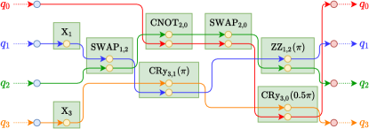
Fig. 4: Example of a graph representation of a quantum circuit with four qubits. The circuit contains gates which are not part of our trapped-ion native gate set $\mathcal{N}$.

4.1 Elimination of SWAP gates

Our shuttling-based ion trap quantum computer natively supports the physical swap of ions [33, 34, 35], which is required to establish full connectivity between the qubits. Thus, in contrast to other gates, SWAP gates are executed by physically swapping ions. In the first compilation step, our compiler replaces the function of SWAP gates by renaming the qubits for all succeeding operations. It is the task of the Shuttling Compiler further downstream in the software stack to generate the corresponding reconfiguration operations.

The process of SWAP gate elimination on the circuit from Fig. 4 is shown in Fig. 5. To eliminate the SWAP gates, the elimination algorithm iterates over the gates $G\in C$ in their execution order. If $G$ is a $\texttt{SWAP}_{i,j}^{k}$ gate acting on the qubits $q_{i}$ and $q_{j}$, $G$ has two subvertices $s_{i}^{k,0}$ and $s_{j}^{k,1}$, respectively. The algorithm exchanges the outgoing edges of these two subvertices. This means that all gates on the path from the input vertex $v_{i}$ to $\texttt{SWAP}_{i,j}^{k}$ are applied to $q_{i}$. Since the outgoing edges of $s_{i}^{k,0}$ and $s_{j}^{k,1}$ have been exchanged, after $\texttt{SWAP}_{i,j}^{k}$ $q_{i}$ follows the path originally taken by $q_{j}$. The same holds for $q_{j}$, which after $\texttt{SWAP}_{i,j}^{k}$ follows the path originally taken by $q_{i}$. Consequently, all gates after $\texttt{SWAP}_{i,j}^{k}$ which were originally executed on $q_{j}$ are now executed on $q_{i}$ and vice versa. In this way, the swap is passed through all gates succeeding $\texttt{SWAP}_{i,j}^{k}$ and the algorithm can eliminate $\texttt{SWAP}_{i,j}^{k}$ from the circuit.

(a) The SWAP gate elimination is applied to the first SWAP gate (the red box). Compared to Fig. 4, the outgoing edges are exchanged. This means that after the SWAP gate, $q_{1}$ follows the green path and $q_{2}$ the blue one. Consequently, the qubits on which the $\texttt{CNOT}_{2,0}$, $\texttt{CRy}_{3,1}\left(\pi\right)$, $\texttt{SWAP}_{2,0}$, and $\texttt{ZZ}_{1,2}\left(\pi\right)$ gates from Fig. 4 act must be adapted to the new qubit. Since all gates on the path of $q_{1}$ and $q_{2}$ after the SWAP gate are adapted to the new qubit following the path, the algorithm can eliminate the SWAP gate from the circuit.

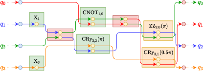
(b) The SWAP gate elimination is also applied to the second SWAP gate (the right red box). Consequently, the outgoing edges are exchanged compared to (a). This means that after the SWAP gate, $q_{0}$ follows the green path and $q_{1}$ the red one.

(c) The circuit after applying the SWAP gate elimination. The orange gates now operate on different qubits than in Fig. 4.

Fig. 5: Applying the SWAP gate elimination to the circuit from Fig. 4.

4.2 Repeated removal and commutation of gates

Our compiler uses Pytket’s RemoveRedundancies pass to remove redundant gates or gate sequences from the circuit. Additionally, our compiler executes Pytket’s CommuteThroughMultis pass to commute gates. When applying commutations, single-qubit gates are commuted through two-qubit gates whenever possible. This may again introduce redundant gates, which can then be removed. The process of commuting and removing gates is repeated until the overall gate count is no longer reduced.

Our compiler executes this transformation step first after the elimination of the SWAP gates, and will also apply it after some of the later transformation stages. The transformation preserves the property that a gate sequence is in the gate set $\mathcal{M}$ or in the gate set $\mathcal{N}$ up to multiples of $\tfrac{\pi}{2}$.

4.3 Macro Matching

Although Pytket provides a transformation for arbitrary gates into the native gate set $\mathcal{M}$, which is used in Sec. 4.4, a custom decomposition gives better results. Therefore, in this step, our compiler applies a predefined decomposition into the native gate set – called macro matching – to the quantum circuit for several gates or gate sequences. This is especially useful for large structured circuits, where known structures can be replaced by beneficial alternatives. Our compiler performs the macro matching transformation only for gates acting on $m\geq 2$ qubits, since efficient transformations exist for local rotations with $m=1$ (see Sec. 4.4). Let $\mathcal{L}$ be a set of gates for which an efficient decomposition is known. All gates from $\mathcal{G}$ contained in $\mathcal{L}$ are replaced by a sequence of gates from $\mathcal{M}$. The gate sequence of the macro is defined in a way that it can be described by the same unitary matrix as the gate $G$, up to a global phase. An example of such a macro is

$$\hskip 2.84526pt\texttt{C\hskip 0.56905ptRy}_{i,j}\left(\theta\right)=\exp\left(-\tfrac{i}{4}\theta(1-Z_{1})Y_{2}\right)$$

$$\ = \hskip 2.84526pt\texttt{Rx}_{j}\left(\tfrac{\pi}{2}\right)\texttt{ZZ}_{i,j}\left(\tfrac{\theta}{2}\right)\texttt{Rz}_{j}\left(-\tfrac{\theta}{2}\right)\texttt{Rx}_{j}\left(\tfrac{3\pi}{2}\right).$$ (7)

Due to the angle restrictions of the gates in $\mathcal{N}$, this macro is only applied if $\theta=\ell\pi$ with $\ell\in\mathbb{Z}$ holds. Otherwise, the original C Ry gate remains in the circuit and will be replaced by the transformations in Sec. 4.4. To simplify the circuit, our compiler executes the repeated removal and commutation of gates from Sec. 4.2 again. The application of the macro matching to the circuit from 5(c) is depicted in Fig. 6.

4.4 Transformation to the native gate set

The predefined gate decomposition into the native gate set by macro matching is followed by the conversion of all remaining gates into the native gate set. Our compiler offers four different approaches for this transformation. While they all start differently, they all end with the RebaseCustom pass to convert the remaining non-native gates.

Fig. 6: Example from 5(c) with the macro matching applied. Since only the gate $\texttt{CRy}_{3,2}\left(\pi\right)$ of the CRy gates in 5(c) satisfies the condition $\theta=\ell\pi$ with $\ell\in\mathbb{Z}$, only this gate is replaced by the orange gates.

The first approach applies Pytket’s CliffordSimp pass to the quantum circuit $C$. This pass contains simplifications similar to those of Duncan and Fagan [38]. After applying the CliffordSimp pass to a circuit, the resulting circuit consists only of Pytket’s universal single-qubit TK1 gates and two-qubit CNOT gates, defined as follows:

$$\texttt{TK1}_{i}\left(\alpha,\beta,\gamma\right) =\texttt{Rz}_{i}\left(\alpha\right)\texttt{Rx}_{i}\left(\beta\right)\texttt{Rz}_{i}\left(\gamma\right),$$ (8a)

$$\texttt{CNOT}_{ij} =\exp\left(i\tfrac{\pi}{4}(I-Z_{i})(I-X_{j})\right).$$ (8b)

Since the CliffordSimp pass also converts ZZ gates with $\theta\in\{\tfrac{\pi}{2},\pi,\tfrac{3\pi}{2}\}$ already contained in $\mathcal{G}$ to a sequence of several TK1 and CNOT gates, our compiler does not apply it directly to the entire circuit $C$, but executes it on subcircuits of $C$ in such a way that ZZ gates with $\theta\in\{\tfrac{\pi}{2},\pi,\tfrac{3\pi}{2}\}$ are preserved. This is advantageous because the $\texttt{ZZ}\left(\tfrac{\pi}{2}\right)$ gates are already part of our trapped-ion native gate set $\mathcal{N}$ and thus would not become shorter. Similarly, $\texttt{ZZ}\left(\pi\right)$ as well as $\texttt{ZZ}\left(\tfrac{3\pi}{2}\right)$ gates can be transformed into smaller gate sequences, see Sec. 4.11. The result of applying the CliffordSimp pass to the example from Fig. 6 can be seen in 7(a).

(a) Example from Fig. 6 after applying Pytket’s CliffordSimp pass. All sequences of single-qubit gates have been replaced by exactly one TK1 gate. Moreover, the $\texttt{CRy}_{3,1}\left(0.5\pi\right)$ gate in Fig. 6 has been transformed into the two orange $\texttt{CNOT}_{3,1}$, the $\texttt{TK1}_{1}\left(0.5\pi,0.25\pi,1.5\pi\right)$ and the $\texttt{TK1}_{1}\left(0.5\pi,1.75\pi,1.5\pi\right)$ gates. Since our compiler executes the CliffordSimp pass so that ZZ gates with $\theta\in\{\tfrac{\pi}{2},\pi,\tfrac{3\pi}{2}\}$ are not converted, $\texttt{ZZ}_{3,2}\left(0.5\pi\right)$ and $\texttt{ZZ}_{2,0}\left(\pi\right)$ remain in the circuit.

(b) Example from Fig. 6 after applying Pytket’s SquashTK1 pass as described in Sec. 4.4. Again, all sequences of single-qubit gates have been replaced by exactly one orange TK1 gate. In contrast to the CliffordSimp pass, the green two-qubit gates remain unchanged.

(c) Circuit after applying Pytket’s RebaseCustom pass as described in Sec. 4.4 to the circuits from (a) and (b). In this case, both circuits result in the same transformed circuit containing only gates from the gate set $\mathcal{M}$. Each CNOT gate has been transformed into exactly one orange ZZ gate and eleven Rz and Rx gates. Additionally, each TK1 gate has been replaced by exactly three Rz and Rx gates. Since the green ZZ gates are still an element of the gate set $\mathcal{M}$ and have an angle $\theta\in\{\tfrac{\pi}{2},\pi,\tfrac{3\pi}{2}\}$, they are the only gates which remain unchanged.

Fig. 7: The process of transforming a circuit into the gate set $\mathcal{M}$.

Sec. 6 shows that the CliffordSimp pass has a nonlinear runtime with the number of gates. To make even large circuits transformable in a reasonable time, a second approach to convert an arbitrary gate sequence to the given native gate set is to execute Pytket’s SquashTK1 pass, which simplifies single-qubit gate sequences. Since this pass does not modify the two-qubit gates, and the built-in rebasing routine used later does not allow to restrict the rotation angles to those contained in our trapped-ion native gate set $\mathcal{N}$, all ZZ gates in $\mathcal{G}$ with $\theta\notin\{\tfrac{\pi}{2},\pi,\tfrac{3\pi}{2}\}$ must be replaced manually. To do this, we use the following decomposition:

$$\texttt{ZZ}_{i,j}\left(\theta\right)= \hskip 2.84526pt\texttt{Rz}_{j}\left(\tfrac{\pi}{2}\right)\texttt{Rx}_{j}\left(\tfrac{\pi}{2}\right)\texttt{ZZ}_{i,j}\left(\tfrac{\pi}{2}\right)$$

$$\cdot \hskip 2.84526pt\texttt{Rz}_{j}\left(\pi\right)\texttt{Rx}_{j}\left(-\theta\right)\texttt{ZZ}_{i,j}\left(\tfrac{\pi}{2}\right)$$

$$\cdot \hskip 2.84526pt\texttt{Rx}_{j}\left(\tfrac{3\pi}{2}\right)\texttt{Rz}_{j}\left(\tfrac{3\pi}{2}\right)\texttt{Rz}_{i}\left(\pi\right).$$ (9)

After the substitution, our compiler executes the repeated removal and commutation of gates from Sec. 4.2 again to simplify the circuit. Then we apply Pytket’s SquashTK1 pass, which converts each sequence of single-qubit gates into exactly one TK1 gate. Applying these substitutions to the example from Fig. 6 results in the circuit shown in 7(b).

Besides these two compilation strategies, there are two other approaches. Both are passes which come with the Pytket package and generally perform well, as shown in Sec. 6. The first approach uses Pytket’s KAKDecomposition pass and performs the KAK decomposition [39] on $C$. The second approach uses Pytket’s FullPeepholeOptimise pass, which executes Clifford simplifications, commutes single-qubit gates, and squashes subcircuits of up to three qubits [40]. Our compiler executes both approaches on the entire circuit $C$, so that the full potential of these optimizations can be exploited on deep circuits.

Regardless of the approach used, the gates in $\mathcal{G}$ are then transformed into the gates in the set $\left\{\texttt{Rx},\texttt{Rz},\texttt{ZZ}\right\}$. This process is called rebasing. For this transformation we use Pytket’s RebaseCustom pass. We found smaller gate counts when excluding the Ry gate, so we excluded Ry from the set. Since $\mathcal{G}$ may contain two-qubit gates which are not ZZ gates when using the approach with Pytket’s SquashTK1 pass, the rebasing first replaces all two-qubit gates which are not ZZ gates with sequences of TK1 and CNOT gates. Then the rebasing replaces the TK1 gates with the definition in (8a) and the CNOT gates with

$$\texttt{CNOT}_{i,j}= \hskip 2.84526pt\texttt{Rz}_{j}\left(\tfrac{\pi}{2}\right)\texttt{Rx}_{j}\left(\tfrac{\pi}{2}\right)\texttt{Rz}_{j}\left(\tfrac{\pi}{2}\right)\texttt{Rz}_{i}\left(\tfrac{\pi}{2}\right)$$

$$\cdot \hskip 2.84526pt\texttt{ZZ}_{i,j}\left(\tfrac{\pi}{2}\right)\texttt{Rx}_{j}\left(\tfrac{\pi}{2}\right)\texttt{Rz}_{j}\left(\tfrac{\pi}{2}\right)$$

$$\cdot \hskip 2.84526pt\texttt{Rx}_{i}\left(\tfrac{\pi}{2}\right)\texttt{Rz}_{i}\left(\pi\right)\texttt{Rx}_{i}\left(\tfrac{\pi}{2}\right).$$ (10)

The decomposition guarantees that the rebasing introduces only ZZ gates with an angle $\theta=\tfrac{\pi}{2}$ into $\mathcal{G}$, so that after applying this transformation all ZZ gates have an angle $\theta\in\{\tfrac{\pi}{2},\pi,\tfrac{3\pi}{2}\}$. After applying the RebaseCustom pass to the circuits from 7(a) and 7(b), the circuit in 7(c) results, which is the same circuit for both approaches in this example.

(a) Example from 7(c) after applying Pytket’s SquashTK1 pass. Each single-qubit gate sequence has been transformed into exactly one orange TK1 gate.

(b) Circuit after applying Pytket’s RebaseCustom pass to the circuit from (a). Each TK1 gate has been transformed into the TK1 decomposition in (8a), which consists of three gates. Since the angles of some gates from the decomposition are zero, and thus these gates are equal to the identity gate, some decompositions have less than three gates.

(c) The circuit from (b) after the Rz gates have been commuted through the ZZ gates and the resulting redundancies have been removed. Consequently, there are at most two single-qubit gates between two ZZ gates on each qubit $q_{i}$ and between the last gate executed on $q_{i}$ and the output vertex of $q_{i}$. Only between the input vertex of $q_{i}$ and the first gate executed on $q_{i}$ three single-qubit gates are possible.

Fig. 8: The process of building Rx-Rz sequences.

4.5 Building Rx-Rz sequences

At this point, the quantum circuit contains only R and Rz gates with arbitrary angle parameters as single-qubit gates and ZZ gates with an angle parameter of $\tfrac{\ell\pi}{2}$ as two-qubit gates. This makes the gate set of the quantum circuit compatible with the native gate set $\mathcal{M}$. Since exactly one TK1 gate can compactly represent any arbitrary sequence of single-qubit gates, the first step is to reduce any sequence of concatenated single-qubit gates to one TK1 gate. Such sequences start and end either at two-qubit gates or at the input or output vertices $v_{i},w_{i}$. The implementation of the algorithm is Pytket’s SquashTK1 pass. It is depicted in 8(a) how this algorithm is applied to the circuit from 7(c). Then we use Pytket’s RebaseCustom pass with (8a) to transform the TK1 gates into gates of set $\mathcal{M}$. The circuit unitary reduced to all gates acting along the path of the qubit $q_{i}$ has the following form:

$$U_{i}=\left(\prod_{\lambda=0}^{\omega_{i}-1}\texttt{Rz}_{i}\texttt{Rx}_{i}\texttt{Rz}_{i}\texttt{ZZ}_{i,j\left(\lambda\right)}\right)\texttt{Rz}_{i}\texttt{Rx}_{i}\texttt{Rz}_{i}.$$ (11)

In this expression, $\omega_{i}$ is the number of ZZ gates executed on $q_{i}$ and $j\left(\lambda\right)$ stands for the qubit $q_{j\left(\lambda\right)}$ on which the ZZ gate $\lambda$ also acts. The circuit from 8(a) after applying the transformation is shown in 8(b). Each path in this circuit has the above structure.

Each ZZ gate $\texttt{ZZ}_{i,j}^{k}\in\mathcal{G}$ is now sandwiched by two Rz gates, which commute with the $\texttt{ZZ}_{i,j}^{k}$ gate on both qubits $q_{i}$ and $q_{j}$. So we can commute the succeeding Rz gates through the ZZ gates and merge with the preceding Rz gates:

$$\texttt{Rz}_{i}(\phi_{s})\texttt{ZZ}_{i,j\left(\lambda\right)}\texttt{Rz}_{i}(\phi_{p})\rightarrow\texttt{ZZ}_{i,j\left(\lambda\right)}\texttt{Rz}_{i}(\phi_{s}+\phi_{p}).$$ (12)

Repeating this procedure, combined with the removal of redundant gates until no further reduction in the number of gates is possible, as described in Sec. 4.2, results in a circuit $C$ in which the disjoint paths of each qubit $q_{i}\in\mathcal{Q}$ have the following form:

(a) Example from 8(c) after applying the transformation of single-qubit gates into our trapped-ion native gate set. The two $\texttt{Rx}_{1}\left(0.25\pi\right)$ gates in 8(c) are transformed into the two orange gate sequences, and their angles are included in the phase of the $\texttt{Rz}_{1}\left(1.25\pi\right)$ gates. All single-qubit gates of the circuit are in our trapped-ion native gate set $\mathcal{N}$.

(b) Circuit from (a) after the Rz gates have been commuted through the ZZ gates and the resulting redundancies have been removed. Since the transformation is applied directly after the Rx-Rz sequences have been built, there are at most four single-qubit gates between two ZZ gates on each qubit $q_{i}$ and between the last gate executed on $q_{i}$ and the output vertex of $q_{i}$. Only between the input vertex of $q_{i}$ and the first gate executed on $q_{i}$ five single-qubit gates are possible.

Fig. 9: The process of transforming the single-qubit gates into our trapped-ion native gate set $\mathcal{N}$.

$$U_{i}=\left(\prod_{\lambda=0}^{\omega_{i}-1}\texttt{Rz}_{i}\texttt{Rx}_{i}\texttt{ZZ}_{i,j\left(\lambda\right)}\right)\texttt{Rz}_{i}\texttt{Rx}_{i}\texttt{Rz}_{i}.$$ (13)

Consequently, on each qubit $q_{i}$ at most one Rx and one Rz gate are executed between two ZZ gates. Let

$$\omega=\frac{1}{2}\sum_{i=0}^{n-1}\omega_{i}$$ (14)

be the number of ZZ gates in $\mathcal{G}$. Thus $\mathcal{G}$ consists of exactly $\omega$ two-qubit gates and at most $4\omega+3n$ single-qubit gates. In 8(c) it is shown how this transformation is applied to the circuit from 8(b).

Rx and Rz with arbitrary angles are the only remaining single-qubit gates in the circuit, and both are also part of $\mathcal{M}$. Since all remaining two-qubit gates are also part of this set, all gates $G_{i}$ of the circuit now satisfy $G_{i}\in\mathcal{M}$.

4.6 Transforming single-qubit gates into our trapped-ion native gate set

Since all gates in the circuit are now part of $\mathcal{M}$, the next step is to make the angles conform to our trapped-ion native gate set $\mathcal{N}$, which has restrictions on the allowed rotation angles. Therefore, all Rx gates must have $\theta\in\left\{\tfrac{\pi}{2},\pi\right\}$. We can use two trivial conversions for $\theta=0$ and $\theta=\tfrac{3\pi}{2}$. In the first case, the gate is equal to the I gate and can be eliminated. In the second case, we can replace the gate by $\texttt{Rx}\left(\tfrac{\pi}{2}\right)\;\texttt{Rx}\left(\pi\right)$.

Rotations Rx with any other values of $\theta$ must be converted into a sequence of Rx gates with allowed rotation angles and Rz gates with freely variable rotation angles. We use the decomposition

$$\hskip 2.84526pt\texttt{Rx}\left(\theta\right)$$

$$= \hskip 2.84526pt\texttt{Rz}\left(\tfrac{\pi}{2}\right)\texttt{Rx}\left(\tfrac{\pi}{2}\right)\texttt{Rz}\left(\theta+\pi\right)\texttt{Rx}\left(\tfrac{\pi}{2}\right)\texttt{Rz}\left(\tfrac{\pi}{2}\right).$$ (15)

After this substitution, the restrictions of our trapped-ion native gate set $\mathcal{N}$ are satisfied for the single-qubit gates. In 9(a) it is shown how the circuit from 8(c) is transformed.

Since our compiler applies this transformation directly after building the Rx-Rz sequences in Sec. 4.5, the unitaries corresponding to the disjoint paths of each qubit $q_{i}$ have the following form:

$$U_{i}= \left(\prod_{\lambda=0}^{\omega_{i}-1}\texttt{Rz}_{i}\texttt{Rz}_{i}\texttt{Rx}_{i}\texttt{Rz}_{i}\texttt{Rx}_{i}\texttt{Rz}_{i}\texttt{ZZ}_{i,j\left(\lambda\right)}\right)$$

$$\cdot \hskip 2.84526pt\texttt{Rz}_{i}\texttt{Rz}_{i}\texttt{Rx}_{i}\texttt{Rz}_{i}\texttt{Rx}_{i}\texttt{Rz}_{i}\texttt{Rz}_{i}.$$ (16)

By again commuting Rz gates through ZZ and combining successive Rz gates according to (12) using the procedures from Sec. 4.2, we can simplify the expression to

$$U_{i}= \left(\prod_{\lambda=0}^{\omega_{i}-1}\texttt{Rz}_{i}\texttt{Rx}_{i}\texttt{Rz}_{i}\texttt{Rx}_{i}\texttt{ZZ}_{i,j\left(\lambda\right)}\right)$$

$$\cdot \hskip 2.84526pt\texttt{Rz}_{i}\texttt{Rx}_{i}\texttt{Rz}_{i}\texttt{Rx}_{i}\texttt{Rz}_{i}.$$ (17)

Consequently, on each qubit $q_{i}$ there are at most two Rx gates and two Rz gates between two ZZ gates. Let $\omega$ be the number of ZZ gates in $\mathcal{G}$ as defined in (14). Thus $\mathcal{G}$ consists of exactly $\omega$ two-qubit gates and at most $8\omega+5n$ single-qubit gates. It is depicted in 9(b) how this transformation is applied to the circuit from 9(a).

Since all R(x) gates now satisfy $\theta\in\left\{\tfrac{\pi}{2},\pi\right\}$, all single-qubit gates are now part of our trapped-ion native gate set $\mathcal{N}$.

Fig. 10: Example from 9(b) after applying the phase tracking algorithm to the circuit. For each Rx gate, the graph contains an R gate depending on the angle of the original gate and the value of the tracking phase $b_{i}$ when the algorithm is applied to the qubit $q_{i}$. The R gates can be simplified to Rx gates if $b_{i}=0$ or Ry gates if $b_{i}=\tfrac{\pi}{2}$. The graph contains no more Rz gates except between the last R gate executed on each qubit $q_{i}$ and the output vertex of $q_{i}$. Consequently, there are at most two R gates between two ZZ gates on each qubit $q_{i}$ and between the input vertex of $q_{i}$ and the first ZZ gate executed on $q_{i}$. Only between the last gate executed on $q_{i}$ and the output vertex of $q_{i}$ two R gates and one Rz gate are possible. Since the values of the tracking phases $b_{1}$ and $b_{3}$ are zero after applying the algorithm to $q_{1}$ and $q_{3}$, no Rz gate is placed before the output vertices of $q_{1}$ and $q_{3}$.

4.7 Phase tracking

We now use the fact that an Rz gate followed by an R gate is equivalent to a single R gate with a phase shifted by the rotation angle of the Rz gate:

$$\texttt{R}\left(\theta,\phi\right)\texttt{Rz}\left(\theta_{z}\right)=\texttt{Rz}\left(\theta_{z}\right)\texttt{R}\left(\theta,\phi-\theta_{z}\right).$$ (18)

Combined with the fact that Rz gates commute through ZZ gates, this allows a virtual execution of all Rz gates using phase tracking [41, 7]. This technique avoids any physical execution of Rz gates and is therefore beneficial in terms of overall runtime and fidelity. All R gates contained in $\mathcal{G}$ must be modified with respect to their phase arguments according to the procedure described in the following.

The algorithm initializes a tracking phase $b_{i}=0$ for each qubit $q_{i}\in\mathcal{Q}$ and follows the path from the input vertex $v_{i}\in\mathcal{V}$ to the output vertex $w_{i}\in\mathcal{W}$. It applies the following rules to each gate $G_{i}\in\mathcal{G}$ it encounters:

• If $G_{i}=\texttt{R}_{i}\left(\theta,\phi\right)$, $G_{i}$ is replaced by $\texttt{R}_{i}\left(\theta,\phi-b_{i}\right)$.

• If $G_{i}=\texttt{Rz}_{i}\left(\phi\right)$, $G_{i}$ is removed from $\mathcal{G}$ and the value of $b_{i}$ is changed to $b_{i}+\phi$.

To correct the final accumulated phase, the algorithm inserts an additional gate $\texttt{Rz}_{i}\left(b_{i}\right)$ into $C$ directly before $w_{i}$. Since the Rz gate only changes the phase of the qubit, the measurement result in the computational basis as performed on the hardware would not be affected. However, adding the Rz gate still has advantages when working with the unitary matrix and when using the circuit as a building block for even larger circuits. An example can be seen in Fig. 10.

Since our compiler executes the phase tracking algorithm immediately after the transformation in Sec. 4.6, the disjoint paths of each qubit $q_{i}\in\mathcal{Q}$ have the following form:

$$U_{i}=\texttt{Rz}_{i}\left(\prod_{\lambda=0}^{\omega_{i}-1}\texttt{R}_{i}\texttt{R}_{i}\texttt{ZZ}_{i,j\left(\lambda\right)}\right)\texttt{R}_{i}\texttt{R}_{i}.$$ (19)

Note that the subsequent R gates generally cannot be merged because they have different phase parameters. Thus, on each qubit, at most two R gates are executed between ZZ gates. Hence, $\mathcal{G}$ consists of exactly $\omega$ two-qubit gates and at most $4\omega+3n$ single-qubit gates. Consequently, phase tracking can almost halve the number of single-qubit gates.

Since phase tracking only changes the phases and not pulse areas, all single-qubit gates are still in $\mathcal{N}$.

4.8 Block aggregations

In this section, we describe further optimization steps which are specific to our shuttling-based architecture. In our architecture, the ions are stored in a linear segmented trap, with qubit subsets stored at different trap segments. Shuttling operations can rearrange the qubit sets between gate operations [9, 6]. Laser beams directed to a fixed location, the laser interaction zone, perform all gate operations. There, each gate operation is executed simultaneously on all stored ions. Hence, identical single-qubit gates can be executed on multiple qubits in parallel. We use this property to reduce the number of gates. As an additional constraint, we keep shuttling operations to a minimum. Thus, we parallelize single-qubit operations only on qubits which are already in the same segment, i. e. before or after a two-qubit gate is executed on them.

Fig. 11: An example circuit with the blocks built by the algorithm from Sec. 4.8. Since the graph contains three ZZ gates, it also contains three blocks, represented by the purple boxes around the ZZ gates. Each block $A\left(\texttt{ZZ}_{i,j}^{k}\right)$ can have a predecessor sequence $p$ and/or a successor sequence $s$. The block $A\left(\texttt{ZZ}_{0,2}^{2}\right)$ contains neither a sequence $p$ nor a sequence $s$ and consists only of the ZZ gate. Besides the three blocks, the graph consists of the seven blockless sequences $b_{0}$ to $b_{6}$.

The optimization described in this section deals with the aggregation of single-qubit gates. It uses the property that there is a specific structure around certain ZZ gates. Directly before and/or directly after a ZZ gate $\texttt{ZZ}_{i,j}^{k}$ there can be sequences of preceding single-qubit gates $p=\left(p_{0},\dots,p_{\alpha-1}\right),p_{0},\dots,p_{\alpha-1}\in C$ and/or succeeding single-qubit gates $s=\left(s_{0},\dots,s_{\beta-1}\right),s_{0},\dots,s_{\beta-1}\in C$ which are similar on both qubits $q_{i},q_{j}\in\mathcal{Q}$ on which the gate $\texttt{ZZ}_{i,j}^{k}$ acts. This means that in these sequences the gates as well as the angle parameters match exactly on $q_{i}$ and $q_{j}$. The advantage of these sequences is that the gates $p_{0},\dots,p_{\alpha-1},s_{0},\dots,s_{\beta-1}$ can be executed simultaneously for both qubits $q_{i}$ and $q_{j}$ instead of sequentially for each qubit, which reduces the execution time and the required shuttling overhead. Each ZZ gate, including the single-qubit gates contained in the sequences $p$ and $s$, build a block $A$. We denote the block belonging to $\texttt{ZZ}_{i,j}^{k}$ as $A\left(\texttt{ZZ}_{i,j}^{k}\right)$ in the following.

Iterating over all ZZ gates in their execution order, the algorithm checks for each gate $\texttt{ZZ}_{i,j}^{k}$ whether $q_{i}$ and $q_{j}$ undergo an identical single-qubit gate $G_{p}$ directly before $\texttt{ZZ}_{i,j}^{k}$. If this is the case and $G_{p}$ does not already belong to another block on $q_{i}$ or $q_{j}$, the algorithm adds $G_{p}$ to the predecessor sequence $p$ of the block $A\left(\texttt{ZZ}_{i,j}^{k}\right)$ and repeats the procedure with the gate directly before $G_{p}$. Otherwise $p$ cannot be increased. The same procedure is repeated with the gates directly after $\texttt{ZZ}_{i,j}^{k}$ to build the sequence $s$ of $A\left(\texttt{ZZ}_{i,j}^{k}\right)$. Since the algorithm traverses the ZZ gates in their execution order, it is guaranteed that candidate gates for $s$ do not already belong to another block. If it is not possible to build $p$ and $s$, the block consists only of $\texttt{ZZ}_{i,j}^{k}$.

An example of the block building process is depicted in Fig. 11. After building such blocks around each ZZ gate $\texttt{ZZ}^{k}\in\mathcal{G}$, there may exist gate sequences $b_{0},\dots,b_{\ell-1}$ which do not belong to a block. Each of these blockless sequences consists only of single-qubit gates and belongs to exactly one qubit. The goal is to minimize the number $\ell$ of blockless sequences.

To minimize the amount and length of blockless single-qubit sequences, the blocks can be rearranged and single-qubit gates can be split. These two approaches are discussed in the following two subsections.

4.8.1 Rearrangement of blocks

A block rearrangement is possible if before a sequence $p$ of a block $A_{\alpha}$ both qubits $q_{i}$ and $q_{j}$ undergo the same gate $G$, but for one qubit, e. g., $q_{j}$, $G$ already belongs to a preceding block $A_{\beta}$ and for $q_{i}$ it belongs to a blockless sequence $b_{\mu}$. Assume $A_{\beta}$ operates on the qubit $q_{j}$ and a third qubit $q_{k}$. If the entire blockless sequence $b_{\mu}$ is equal to the end $s_{e}$ of the sequence $s$ of the block $A_{\beta}$, the gates of $b_{\mu}$ and $s_{e}$ acting on the qubit $q_{j}$ are appended to the front of the sequence $p$ of $A_{\alpha}$. Consequently, the blockless sequence $b_{\mu}$ is eliminated and the gates of $q_{j}$ in $s_{e}$ are removed from $s_{e}$, see 12(a) and 12(b).

(a) The same gate sequences $b_{\mu}$ and $s_{e}$ are executed on $q_{1}$ and $q_{3}$ before the block $A_{\alpha}$. On $q_{1}$ the gate sequence $b_{\mu}$ is a blockless sequence, while on $q_{3}$ the gate sequence $s_{e}$ belongs to a different block $A_{\beta}$. To eliminate the blockless sequence $b_{\mu}$, $b_{\mu}$ and the gates on $q_{3}$ from $s_{e}$ can be added as a predecessor sequence to $A_{\alpha}$.

(b) $b_{\mu}$ and the gates on $q_{3}$ from $s_{e}$ have been added as predecessor sequence $p$ to $A_{\alpha}$. Consequently, the gates on $q_{2}$ from $s_{e}$ now build a new blockless sequence $b_{\nu}$. This blockless sequence is identical to the blockless sequence $b_{\xi_{e}}$ on $q_{0}$. Since $b_{\nu}$ and $b_{\xi_{e}}$ are both directly in front of a third block $A_{\gamma}$, they can be added as predecessor sequence to $A_{\gamma}$.

(c) $b_{\mu}$ and $b_{\xi_{e}}$ have been added as predecessor sequence $p$ to $A_{\gamma}$. By rearranging the blocks, the graph now has one blockless sequence less than in (a).

(d) In (c) the same gates are executed before the block of gate $\texttt{ZZ}^{0}_{0,1}$ and after the block of gate $\texttt{ZZ}^{2}_{0,2}$, but with different pulse areas $\theta$. Using the angle splitting approach, the gate with the larger angle is replaced by the two orange gates. Since the orange gate next to the ZZ gate and the blue gate have the same angle, these two gates can be added to the block. This eliminates two blockless sequences in this example. The two R gates before the block of gate $\texttt{ZZ}^{1}_{2,3}$ cannot be used for angle splitting because the phase $\phi$ is different.

Fig. 12: The process of rearranging blocks and splitting angles.

Since only the gates of the qubit $q_{j}$ in $s_{e}$ are removed from $s_{e}$, the gates of the qubit $q_{k}$ in $s_{e}$ result in a new blockless sequence $b_{\nu}$. To eliminate $b_{\nu}$, it is necessary that $b_{\nu}$ is adjacent to a third block $A_{\gamma}$ operating on the qubit $q_{k}$ and a qubit $q_{l}$. Here the case $q_{i}=q_{l}$ is possible. If before the sequence $p$ of $A_{\gamma}$ there is a blockless sequence $b_{\xi}$ on the qubit $q_{l}$ with the sequence $b_{\nu}$ at the end, the procedure appends $b_{\nu}$ and $b_{\xi_{e}}$ to the front of $p$ of $A_{\gamma}$ and the number of blockless sequences on the circuit is reduced by one. This can be seen in 12(b) and 12(c). If minimizing the number of blockless sequences is not possible because a matching sequence is missing during the algorithm, the blocks are not rearranged. We repeat the rearranging procedure for all blocks on which a rearrangement is possible.

4.8.2 Angle splitting

After the rearrangement, the number of blockless sequences might be further reduced by splitting the rotation angles of certain gates. Assume that before a sequence $p$ or directly after a sequence $s$ of a block $A\left(\texttt{ZZ}_{i,j}^{k}\right)$ both qubits $q_{i}$ and $q_{j}$ undergo rotations $\texttt{R}_{i}(\theta_{i},\phi)$ and $\texttt{R}_{j}(\theta_{j},\phi)$ with the same phase angle but different rotation angles. Then it is possible to split the gate with the larger rotation angle into two rotations, merge the resulting two identical gates into the respective set $s$ or $p$ of the block, and eventually reduce the number of blockless sequences. The phase angle is omitted from the notation in the following.

We now assume that $G_{i}\left(\theta_{i}\right)$ belongs to the blockless sequence $b_{i}$ and $G_{j}\left(\theta_{j}\right)$ belongs to the blockless sequence $b_{j}$, and that both $b_{i}$ and $b_{j}$ either directly precede or directly succeed block $A$. We also assume without loss of generality that $\theta_{i}<\theta_{j}$. The gate $G_{j}\left(\theta_{j}\right)$ can be split into two consecutive gates $G_{j}\left(\theta_{i}\right)\;G_{j}\left(\theta_{j}-\theta_{i}\right)$, so that a simultaneous gate $G(\theta_{i})$ can be merged into either $p$ or $s$. In the former case, the procedure appends $G\left(\theta_{i}\right)$ to the front of $p$, while in the latter case, it appends $G\left(\theta_{i}\right)$ to the end of $s$. In both cases, the procedure removes $G_{i}(\theta_{i})$ from $b_{i}$, and within $b_{j}$ it replaces $G_{j}(\theta_{j})$ with $G_{j}(\theta_{j}-\theta_{i})$. This reduces the blockless sequence $b_{i}$ by one gate and eliminates $b_{i}$ if it is now empty. If this is not the case and $b_{i}$ cannot be eliminated, the procedure rejects the transformation step and keeps the initial gates $G_{i}\left(\theta_{i}\right)$ and $G_{j}\left(\theta_{j}\right)$. We repeat the procedure until no more block $A$ can be increased. The execution of the angle splitting approach on the circuit from 12(c) is shown in 12(d).

Afterwards, our compiler transforms all blockless sequences which cannot be completely eliminated according to Sec. 4.4 so that they consist of a minimal number of native gates from $\mathcal{N}$. The same transformations are applied to the sequences $p$ and $s$ of each block $A$ to minimize the number of gates used.

Note that before angle splitting the circuit consists only of gates with rotation angles $\theta\in\left\{\tfrac{\pi}{2},\pi\right\}$, so angle splitting preserves the property that all gates are contained in the set of allowed gates $\mathcal{N}$.

4.9 Commutations of blocks and blockless sequences on disjoint sets of qubits

The previous compilation steps ensure that the gates acting on a certain qubit are executed in a function receiving order. However, these compilation steps are not optimized for the shuttling overhead, and this generally results in an unfavorable order of blocks and blockless sequences. We now describe how the execution order of blocks and blockless sequences can be rearranged to reduce the amount of shuttling operations required. We exploit the property that the execution order of two blocks or blockless sequences can be swapped if they act on disjoint sets of qubits. The approach then tries to commute each blockless sequence so that it is executed immediately before or after a block applied to the same qubit. An example of such a rearrangement is shown in Fig. 13.

(a) The gates are executed in a semi-random order, taking care only that on each qubit $q_{i}$ a gate $G$ is executed after all gates placed before $G$ on $q_{i}$ have been executed.

(b) The commutations have been applied. Blockless sequences of a qubit $q_{i}$ are always executed directly before or after a block acting on $q_{i}$. Moreover, since the Blocks 8 and 11 act on the same qubits, they are executed successively only with the blockless sequences 9 and 10 in between. Since the Blocks 3 and 14 have only $q_{1}$ in common, blockless sequence 5 is executed after blockless sequence 4. Additionally, blockless sequence 13 is executed after blockless sequence 12 because the Blocks 11 and 14 have only $q_{2}$ in common. The order of the blockless sequences in all other pairs executed before or after a block is arbitrary. E. g., the order of the blockless sequences 1 and 2 can be reversed.

Fig. 13: Example of applying the commutation of blocks and blockless sequences on disjoint sets of qubits to a circuit. The purple boxes represent blocks and the yellow boxes represent blockless sequences. The numbers inside the boxes indicate the order in which the gates are executed, i. e. the gate with the number 1 is executed first, then the gate with the number 2, and so on.

Now assume that two blockless sequences $b_{i}$ and $b_{j}$ are executed after a block $A_{\alpha}$ and that $A_{\alpha}$ acts on the qubits $q_{i},q_{j}\in\mathcal{Q}$ and $b_{i}$ is applied to $q_{i}$ and $b_{j}$ is applied to $q_{j}$. The algorithm now iterates over the initial execution order of the circuit, searching for the next block $A_{\beta}$ which acts on either $q_{i}$ or $q_{j}$ after $A_{\alpha}$. If none exists, the order of $b_{i}$ and $b_{j}$ may be arbitrary. If $A_{\beta}$ is applied to $q_{i}$ and not to $q_{j}$, then $b_{j}$ is executed before $b_{i}$. The analogous rule holds if $A_{\beta}$ acts on $q_{j}$ and not on $q_{i}$. Moreover, if $A_{\beta}$ acts on $q_{i}$ and $q_{j}$, the algorithm commutes $A_{\beta}$ so that it is executed immediately after $A_{\alpha}$, with only $b_{i}$ and $b_{j}$ in between. In this way, blocks which operate on exactly the same qubits are executed successively if possible.

4.10 Block commutations with correction unitaries

In the last subsection we have commuted blocks and blockless sequences acting on disjoint sets of qubits. In this subsection, we present an additional algorithm which commutes superblocks with the following properties: Each superblock consists of at least one two-qubit gate and can consist of several single-qubit gates. All gates of the superblock must operate on the same two qubits and must be executed consecutively on these qubits. For the commutation, the algorithm needs two superblocks with exactly one qubit in common, so that the commutation affects gates on three qubits. Between the two superblocks, no gate may affect the common qubit. The commutation of the superblocks is performed in such a way that afterwards subsequent superblocks in the execution order should operate on the same qubits or have at least one qubit in common. If possible, these commutations can increase the number of such sequences and thus reduce the shuttling overhead.

The order of blocks with unitaries of size $\nu\times\nu$ with $\nu\in\mathbb{N}$ cannot simply be swapped, because the corresponding matrix multiplications are non-commutative. Consequently, the commutation of the unitaries associated with the superblocks introduces an error into the circuit. To correct the error, a correction unitary is inserted into the circuit after commutation. It is placed behind the superblocks and operates on the same three qubits as the two superblocks. However, the correction unitary can insert two-qubit gates between all three qubits, breaking the structure that the gates operate only between the qubits of their superblock. To prevent this, we show that under certain conditions the correction unitary can be factorized into two correction unitaries. While one of the unitaries is applied only to one of the qubits which is not the common qubit, the other unitary is applied to the other two qubits which then act on the same superblock. This guarantees that the correction unitaries introduce at most two-qubit gates between these two qubits. If the correction unitary does not factorize, the presented algorithm rejects the commutation of the superblocks. An example is shown in Fig. 14.

(a) Example from 13(b) with the superblocks $B_{\beta}$ and $B_{\gamma}$. The non-yellow blockless sequences can be added completely, partially or not to the adjacent superblocks. Since no gates are allowed on the common qubit $q_{2}$ between the two superblocks, blockless sequence 13 must be added completely to $B_{\beta}$ or $B_{\gamma}$ or divided between them.

(b) The superblock $B_{\beta}$ has been commuted before $B_{\gamma}$ and the correction unitaries $U^{\prime}_{q_{1}}$ and $U^{\prime}_{q_{2}q_{3}}$ (the dark gray boxes) has been inserted into the circuit. The brown, red, green, and light gray colors indicate to which blockless sequences the corresponding blockless sequences from (a) can be transformed, depending on whether they have been added completely, partially, or not to a superblock, and how they are ordered in the new blockless sequences. The commutation leads to a step-shaped arrangement of the gates, which further reduces the number of shuttling operations.

Fig. 14: Example of applying the block commutation with correction unitaries to a circuit. While the purple boxes represent the blocks built during block building in Sec. 4.8, the blue boxes represent the superblocks to be swapped, and the dark gray boxes are the correction unitaries. All other boxes are blockless sequences. Analogous to Fig. 13, the numbers inside the boxes indicate the order in which the gates are executed.

In Sec. 4.10.1 the detailed theory of the block commutation with correction unitaries is described. Afterwards, in Sec. 4.10.2 an algorithm for the execution of the block commutation with correction unitaries is presented. This is followed by a heuristic in Sec. 4.10.3 to measure the impact of the block commutation with correction unitaries on the shuttling operations independently of a concrete implementation of a Shuttling Compiler.

4.10.1 Theory of the block commutation with correction unitaries

Fig. 15: The two superblocks represented by the unitaries $U_{q_{i}q_{j}}^{(\beta)}$ and $U_{q_{j}q_{k}}^{(\gamma)}$ are commuted. Since in general it is not guaranteed that both unitaries are commutable, a correction unitary $U^{\prime}$ is inserted, which corrects the error introduced by the commutation of the superblocks. Under certain conditions $U^{\prime}$ can be factorized into two correction unitaries $U^{\prime}_{q_{i}}$ and $U^{\prime}_{q_{j}q_{k}}$.

We consider two consecutive superblocks $B_{\beta}$ acting on the qubits $q_{i},q_{j}\in\mathcal{Q}$ and $B_{\gamma}$ acting on $q_{j},q_{k}\in\mathcal{Q}$, resulting in the three-qubit unitary

$$U=U_{q_{i}q_{j}}^{(\beta)}U_{q_{j}q_{k}}^{(\gamma)},$$ (20)

where $U_{q_{i}q_{j}}$ is the unitary associated with $B_{\beta}$ and $U_{q_{j}q_{k}}$ is the unitary associated with $B_{\gamma}$. Consecutive in this context means that no gates may be executed on the common qubit $q_{j}$ between the two superblocks. It can be beneficial to reverse the execution order of the superblocks to reduce the shuttling overhead. In this section, we show how to determine the conditions under which the execution order can be reversed. In general, the reversal requires a correction unitary $U^{\prime}$ to obtain the same total unitary:

$$U=U^{\prime}U_{q_{j}q_{k}}^{(\gamma)}U_{q_{i}q_{j}}^{(\beta)}.$$ (21)

The three-qubit correction unitary is given by

$$U^{\prime} =U_{q_{i}q_{j}}^{(\beta)}U_{q_{j}q_{k}}^{(\gamma)}U_{q_{i}q_{j}}^{(\beta)\dagger}U_{q_{j}q_{k}}^{(\gamma)\dagger}.$$ (22)

Given $U_{q_{i}q_{j}}^{(\beta)}$ and $U_{q_{j}q_{k}}^{(\gamma)}$ in matrix form, we need to check if $U^{\prime}$ factorizes into a $q_{i}/q_{j}q_{k}$ separable form:

$$U^{\prime}=U_{q_{i}}^{\prime}\otimes U_{q_{j}q_{k}}^{\prime}.$$ (23)

We explicitly compute $U^{\prime}$ and use the set of Pauli operators for a single-qubit $\mathcal{P}_{q}=\left\{I_{q},X_{q},Y_{q},Z_{q}\right\}$ to decompose it into single-qubit Pauli operators acting on $q_{i}$ and two-qubit Pauli operators acting on $q_{j}$ and $q_{k}$:

$$U^{\prime}=\sum_{P_{\lambda}\in\mathcal{P}_{q_{i}}}\sum_{P_{\mu}\in\mathcal{P}_{q_{j}}\otimes\mathcal{P}_{q_{k}}}M_{\lambda\mu}P_{\lambda}\otimes P_{\mu}.$$ (24)

Note that the $P_{\mu}$ are two-qubit unitaries from the tensor product set $\mathcal{P}_{q_{j}}\otimes\mathcal{P}_{q_{k}}$. The decomposition results in a $4\times 16$ matrix $M$ with the entries

$$M_{\lambda\mu}=\frac{1}{8}\operatorname{tr}\left(U^{\prime}\;P_{\lambda}\otimes P_{\mu}\right),$$ (25)

which has the singular value decomposition

$$M=USV^{\dagger}$$ (26)

with the $4\times 4$ and $16\times 16$ unitary matrices $U$ and $V$. The $4\times 16$ matrix $S$ consists of a $4\times 4$ diagonal matrix on the left, whose non-zero entries are the singular values of $M$, and a $4\times 12$ zero matrix on the right. If $\operatorname{rank}S=1$, only $S_{11}\neq 0$ and $U^{\prime}$ factorizes according to (23). The resulting correction unitaries are given by

$$U^{\prime}_{q_{i}} =\sum_{\lambda=1}^{4}U_{\lambda,1}P_{\lambda},$$ (27a)

$$U^{\prime}_{q_{j}q_{k}} =\sum_{\mu=1}^{16}V_{\mu,1}^{*}P_{\mu}.$$ (27b)

The final unitary in favorable order is

$$U=U^{\prime}_{q_{j}q_{k}}U_{q_{j}q_{k}}^{(\gamma)}U^{\prime}_{q_{i}}U_{q_{i}q_{j}}^{(\beta)},$$ (28)

which contains $U_{q_{i}q_{j}}$ and $U_{q_{j}q_{k}}$ in the commuted order compared to (20). A visualization of the commutation is given in Fig. 15.

4.10.2 Algorithm for executing the block commutation with correction unitaries

In the following, we describe the algorithm for performing the block commutation with correction unitaries on an input circuit $C$. While for the theory in Sec. 4.10.1 we assumed that the superblocks are already known, in practice the algorithm must first determine the superblocks on the circuit. Therefore, a block from Sec. 4.8 forms the basis of each superblock, which is enlarged in a second step. The blocks are chosen to reduce the number of shuttling operations required. The algorithm iterates over the blocks and blockless sequences in their execution order. It searches for three blocks $A_{\alpha}$, $A_{\gamma}$, and $A_{\beta}$, where $A_{\gamma}$ and $A_{\beta}$ are the base blocks of the superblocks $B_{\gamma}$ and $B_{\beta}$, respectively. $A_{\alpha}$ is the block executed directly before $B_{\gamma}$ in the execution order and has at least one qubit in common with $B_{\beta}$. Thus, commuting $B_{\gamma}$ and $B_{\beta}$ places $B_{\beta}$ between $A_{\alpha}$ and $B_{\gamma}$ regarding the execution order and ensures that after the commutation, $A_{\alpha}$ and $B_{\beta}$ are executed successively with at least one qubit in common. Consequently, this may lead to better locality during shuttling and reduce the shuttling overhead.

At the beginning, the algorithm searches for the block $A_{\alpha}$, which is the first block found in the execution order during the iteration. The block following $A_{\alpha}$ in the execution order is used as $A_{\gamma}$ acting on the qubits $q_{j}$ and $q_{k}$ and as the basis for the superblock $B_{\gamma}$. If $A_{\alpha}$ and $A_{\gamma}$ act on exactly the same qubits, $A_{\gamma}$ becomes the new $A_{\alpha}$ and the algorithm searches for a new $A_{\gamma}$. This ensures that the locality of acting on common qubits between both blocks is not broken.

If $A_{\alpha}$ and $A_{\gamma}$ act on at least one different qubit, the algorithm searches for the block $A_{\beta}$ as the basis for the superblock $B_{\beta}$. To perform the commutation as described in Sec. 4.10.1, $A_{\beta}$ needs exactly one common qubit, $q_{j}$, with $A_{\gamma}$. Since $B_{\beta}$ immediately follows $A_{\alpha}$ in the execution order after commutation, $A_{\beta}$ must also have at least $q_{i}$ in common with $A_{\alpha}$ to reduce the shuttling overhead. When searching for $A_{\beta}$, it need not be the direct successor block of $A_{\gamma}$ in the execution order. It is possible that there are other blocks between $A_{\gamma}$ and $A_{\beta}$. We use the intermediate blocks which act on $q_{j}$ and $q_{k}$ later to extend $B_{\gamma}$, as long as there is no other block which acts only on $q_{j}$ or $q_{k}$ in the execution order. The other intermediate blocks must not have a qubit in common with $A_{\beta}$ to guarantee that $A_{\beta}$ commutes with them. If $A_{\alpha}$ has exactly one qubit in common with $A_{\beta}$ and $A_{\gamma}$, a commutation of $B_{\beta}$ between $A_{\alpha}$ and $B_{\gamma}$ does not cause $A_{\alpha}$ to be followed by a block which has more qubits in common with $A_{\alpha}$ than $A_{\gamma}$. Nevertheless, the commutation is performed in this case because it may allow $B_{\beta}$ to be commuted with another commutation before $A_{\alpha}$, which may lead to better locality in shuttling. If a block $A_{\beta}$ cannot be found, $A_{\gamma}$ becomes the new $A_{\alpha}$ and the algorithm continues to search for a new $A_{\gamma}$.

After our algorithm has determined the base gates of the superblocks, there are two ways to extend them. First, a neighboring block from the blocks built during block aggregation can be merged into a superblock if it operates on the same qubits as the superblock and there is no other block between it and the superblock which operates on only one of the qubits. If another block is added to a superblock, all blockless sequences operating on the same qubits between the added block and the superblock also become part of the superblock.

The second way is to extend the superblocks by their neighboring blockless sequences or parts of them which act on a qubit of the corresponding superblock. While in general we can add blockless sequences completely or only some gates of them, there are two exceptions where the algorithm always adds blockless sequences completely to the adjacent superblock. Both exceptions have in common that the blockless sequence is executed directly before or after $B_{\beta}$ on $q_{i}$ or $B_{\gamma}$ on $q_{k}$ in the execution order. However, in the first case, the block before or after the blockless sequence in the execution order does not act on the same qubit as the blockless sequence. On the other hand, in the second case, the blockless sequence contains the first or last gates of the corresponding qubit in the circuit. Adding these blockless sequences to the superblocks leads to better locality during shuttling. All other blockless sequences which do not fall under these exceptions can be divided into two parts. When the algorithm divides a blockless sequence, only the gates closer to the superblock are added, while the other part remains outside the superblock. It is possible that one of the parts does not consist of a gate, which means that depending on the part, the entire blockless sequence may or may not be added to the superblock. An exception is the blockless sequence on the common qubit $q_{j}$ between the two superblocks. Since no gate is allowed at this position, this blockless sequence must be added to one of the superblocks. Therefore, it can be added completely to either $B_{\beta}$ or $B_{\gamma}$, or it can be divided so that one part is added to $B_{\beta}$ and the other part to $B_{\gamma}$.

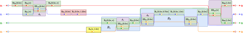
(a) Example from Fig. 10 after applying block aggregation and the commutation of blocks and blockless sequences on disjoint sets of qubits. The purple boxes represent the blocks built by block aggregation. The left-to-right order of the gates determined by the commutation of blocks and blockless sequences on disjoint sets of qubits describes the execution order of the gates. When the algorithm in Sec. 4.10.2 is executed, it first finds the block $A_{\alpha}$ acting on $q_{0}$ and $q_{1}$, and $A_{\gamma}$ acting on $q_{2}$ and $q_{3}$. Since the third block, $A_{\beta}$, has $q_{1}$ in common with $A_{\alpha}$ and $q_{3}$ in common with $A_{\gamma}$, it can be used for the block commutation with correction unitaries. The blocks $A_{\gamma}$ and $A_{\beta}$ are the basis for the superblocks $B_{\gamma}$ and $B_{\beta}$, respectively. Expanding the base superblocks with other blocks and the blockless sequences, which are always added to the superblocks, results in the displayed blue superblocks $B_{\gamma}$ and $B_{\beta}$. However, it is not guaranteed that the blue blocks are commutable. It is possible to further enlarge $B_{\gamma}$ with the yellow gate and $B_{\beta}$ with the red gates. In the case of $B_{\beta}$, it is possible to add only the right red gate or both red gates. The value of the heuristic in Sec. 4.10.3 for this circuit is one.

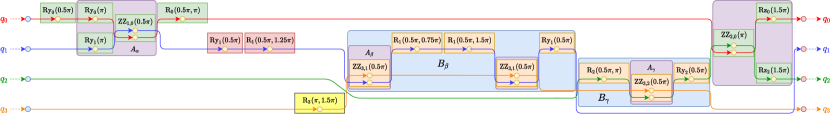
(b) Circuit from (a) after commuting $B_{\beta}$ before $B_{\gamma}$. Since $U^{\prime}_{q_{1}}$ and $U^{\prime}_{q_{3}q_{2}}$ are identity matrices, no additional gates have been added to the circuit. The commutation has been performed without adding the red and yellow gates to their corresponding superblocks. While adding the right red gate or both red gates to $B_{\beta}$ would have produced the same result as without adding, adding the yellow gate to $B_{\gamma}$ would have made the commutation unexecutable regardless of how many red gates were added to $B_{\beta}$. The value of the heuristic in Sec. 4.10.3 for this circuit is $\tfrac{4}{3}$. In contrast to the circuit in (a), where the successive blocks $A_{\alpha}$ and $A_{\gamma}$ act on completely different qubits, after commutation each block has at least one qubit in common with its predecessor block, making the operations more local.

Fig. 16: The process of applying the block commutation with correction unitaries.

To find the best partitioning of the dividable blockless sequences, our algorithm determines all possible partitionings of these sequences. Afterwards, for both superblocks, each partitioning of each dividable blockless sequence is combined with each partitioning of the other blockless sequences. In this way, we build several candidate superblocks for $B_{\beta}$ and $B_{\gamma}$. Then we compute the unitary matrices of each candidate superblock of $B_{\beta}$ and $B_{\gamma}$, and the procedure in Sec. 4.10.1 is executed for each possible combination of a candidate superblock of $B_{\beta}$ with a candidate superblock of $B_{\gamma}$. Due to the generally intertwined structure of the circuit archived by the previous compilation steps, there are only a few combinations to execute. Thus, it is not computationally infeasible to check all combinations for a typical case. In 16(a) it is depicted how our algorithm builds superblocks in the example from Fig. 10 and how they can be extended.

For all combinations where $U^{\prime}$ factorizes, our algorithm transforms the unitaries $U^{\prime}_{q_{i}}$ and $U^{\prime}_{q_{j}q_{k}}$ into circuits using Pytket. We then optimize these circuits using our compilation flow up to phase tracking and using the FullPeepholeOptimise pass in Sec. 4.6.

If there are multiple combinations for which $U^{\prime}$ factorizes, the algorithm determines which combination to use for the commutation. Therefore, several heuristics can be used, depending on the optimization goal, such as minimizing the overall gate count or the two-qubit gate count. We present three such heuristics in the following. The first heuristic prioritizes the reduction of the overall gate count over the minimization of the two-qubit gate count as the optimization goal. The heuristic is applied top-down. If multiple combinations satisfy a criterion, the next criterion is used for further selection:

1. Select the combination(s) with the smallest total number of gates in the circuits of $U^{\prime}_{q_{i}}$ and $U^{\prime}_{q_{j}q_{k}}$.

2. Select the combination(s) with the lowest number of two-qubit gates in $U^{\prime}_{q_{j}q_{k}}$.

3. Select the combination(s) with the lowest number of blockless sequences.

4. Select one combination randomly.

The second heuristic reverses the first two criteria, giving priority to reducing the two-qubit gate count over minimizing the overall gate count. A middle ground between the two heuristics is the third heuristic, which uses the same order of the criteria as the first heuristic. However, when counting the number of gates in $U^{\prime}_{q_{i}}$ and $U^{\prime}_{q_{j}q_{k}}$, each two-qubit gate is counted as $\xi>1$ gates. This way the two-qubit gates have a higher weight in the gate count, prioritizing combinations with a lower number of two-qubit gates, but without completely ignoring the single-qubit gates in the first criterion as in the second heuristic.

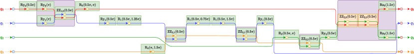
Fig. 17: Example from 16(b) after applying the transformation of two-qubit gates into our trapped-ion native gate set. The $\texttt{ZZ}_{2,0}\left(\pi\right)$ gate in 16(b) is transformed into the two orange $\texttt{ZZ}_{2,0}\left(0.5\pi\right)$ gates. All gates of the circuit are in our trapped-ion native gate set $\mathcal{N}$.

We then commute $B_{\beta}$ and $B_{\gamma}$ with respect to the selected combination and insert the gates from $U^{\prime}_{q_{i}}$ and $U^{\prime}_{q_{j}q_{k}}$ into the circuit $C$. In the following, our algorithm treats each two-qubit gate contained in the circuit of $U^{\prime}_{q_{j}q_{k}}$ as a block containing only the corresponding gate, while it combines the inserted single-qubit gates into blockless sequences. As an example, 16(b) shows the circuit from 16(a) with commuted superblocks.

To further determine possible superblocks for commutation, the algorithm selects the new $A_{\alpha}$ in such a way that $A_{\beta}$ can serve as $A_{\beta}$ again and can be commuted again. If this is not possible, the algorithm uses the first block in the execution order of the circuit as the new $A_{\alpha}$. This allows a recursive commutation of blocks, which leads to a nonlinear runtime of the block commutation with correction unitaries. To avoid that the blocks are commuted cyclically, we check that the same two blocks are not commuted twice.

If the algorithm cannot find any more commutations and has performed at least one commutation, we optimize the circuit with the commuted blocks. Therefore, we remove the block aggregations of Sec. 4.8. Due to the commutations, it is possible that more than two R gates act on the same qubit between two ZZ gates. We apply Pytket’s SquashTK1 pass and the RebaseCustom pass to these sequences. Then we re-run our compilation flow from the transformation pass in Sec. 4.6. This removes the Rx gates introduced by the circuits of $U^{\prime}_{q_{i}}$ and $U^{\prime}_{q_{j}q_{k}}$ as well as the rebasing pass which do not have an angle of $\frac{\pi}{2}$ or $\pi$. Furthermore, phase tracking eliminates the newly introduced Rz gates and the block aggregation builds new blocks considering the new optimizations. The new blocks and blockless sequences acting on disjoint sets of qubits are then commuted as described in Sec. 4.9.

4.10.3 Heuristic evaluation of the commutation

The algorithm presented above puts the circuit into a favorable structure by commuting superblocks. However, the algorithm does not measure the impact of the commutations on the shuttling operations. To allow our compiler to be used independently of a concrete implementation of a Shuttling Compiler, we present a heuristic for evaluating the impact of the commutations. We calculate this heuristic for the circuit before and after applying the block commutation with correction unitaries. The circuit with the higher heuristic value is used for the further compilation.

To compute the heuristic, the algorithm iterates over the entire circuit in the execution order, looking at each pair of consecutive blocks built in Sec. 4.8. For each pair, the algorithm determines how many qubits the blocks have in common. These amounts are added and divided by the number of pairs. The result is a value between zero and two. The heuristic can only reach a value of zero if each block affects two different qubits compared to its immediate predecessor block in the execution order. This means that the blocks are in the most unfavorable order. In contrast, the heuristic can only reach a value of two if all blocks operate on the same two qubits. Consequently, reaching a value of two is not possible for circuits where the block commutation with correction unitaries has been applied, because it is only applicable to circuits where gates act on at least three different qubits.

Using the block commutation with correction unitaries should increase the value of the heuristic. The higher the value, the more blocks following each other in the execution order will have qubits in common and the more local the operations will be. As a result, the number of shuttling operations will decrease. See Fig. 16 for an example of using the heuristic.

4.11 Transformation of two-qubit gates into our trapped-ion native gate set

The transformation in Sec. 4.4 has converted the ZZ gates so that they have a phase $\theta\in\left\{\tfrac{\pi}{2},\pi,\tfrac{3\pi}{2}\right\}$. Since our trapped-ion native get set $\mathcal{N}$ contains only the gate $\texttt{ZZ}\left(\tfrac{\pi}{2}\right)$, the ZZ gates in $\mathcal{G}$ with a phase of $\pi$ or $\tfrac{3\pi}{2}$ must be transformed to satisfy the condition. Therefore, the following decomposition is used:

$$\texttt{ZZ}\left(\pi\right) =\texttt{ZZ}\left(\tfrac{\pi}{2}\right)\texttt{ZZ}\left(\tfrac{\pi}{2}\right),$$ (29a)

$$\texttt{ZZ}\left(\tfrac{3\pi}{2}\right) =\texttt{ZZ}\left(\tfrac{\pi}{2}\right)\texttt{ZZ}\left(\tfrac{\pi}{2}\right)\texttt{ZZ}\left(\tfrac{\pi}{2}\right).$$ (29b)

This transformation is applied to the circuit from 16(b) in Fig. 17.

Note that this transformation could also have been applied earlier. However, not only would there be no benefit, but it would also worsen the runtimes of the block aggregation and the commutations because there are more two-qubit gates to consider. It should also be noted that the single-qubit gates are already part of our trapped-ion native gate set $\mathcal{N}$, and since the two-qubit gates are as well, the circuit $C$ is now executable on the target quantum computing architecture.

5 Parameterized Circuits

Important applications of quantum processors in the NISQ era include quantum machine learning [42] and Variational Quantum Eigensolver (VQE) algorithms [43]. These use cases require a parameterized circuit to be executed multiple times with only small variations in some gate parameters, i. e. phases and angles of the gates. A classical optimizer then compares and adjusts the results of these executions. To make the circuits comparable, it is important that their structure is identical. However, different gate parameters can lead to different circuits after applying the compilation steps of our paper. Introducing the compilation of parameterized circuits mitigates this problem. Whenever unresolved parameters are present in the circuit to be compiled, these parameters are preserved throughout the compilation and only generally applicable optimizations are performed. Pytket natively supports such parameterized compilation and generates parameter-dependent expressions for all its transformations.

When compiling parameterized circuits, our compiler still removes all SWAP gates (Sec. 4.1) and the gates that cancel out (Sec. 4.2), but only if the cancellation is independent of the current parameters. Additionally, macro matching is performed (Sec. 4.3) only if all values of the parameters satisfy the macro condition. The same scheme is also applied to all following steps. The final circuit may contain gates with angles and phases defined by non-trivial mathematical expressions, mainly introduced when transforming the circuit into our native gate set (Sec. 4.4). While compiling parameterized circuits does not restrict phase tracking (Sec. 4.7), block aggregation (Sec. 4.8) and the block commutation with correction unitaries (Sec. 4.10) lose much of their impact. The latter is not performed for parameterized circuits for performance reasons.

As an example, we used [44] to generate a parameterized circuit representing a Unitary Coupled Cluster ansatz [45], which is needed when executing variational algorithms such as VQE [46]. The circuit has four qubits, 48 single-qubit and 32 two-qubit gates, and contains two parameters. When we compiled the circuit together with the parameters into our trapped-ion native gate set, we got a circuit with 69 single-qubit and 32 two-qubit gates. In this circuit, the parameters can be replaced by numeric values to get executable circuits. This allows us to execute the circuit with different values after compiling it once. If the values are known before compilation and the circuit only needs to be executed with these values, the parameters can be replaced before compilation. In this case, we got a circuit with 61 single-qubit and 32 two-qubit gates. The small increase factor of 1.13 in the number of single-qubit gates for the parameterized compilation compared to the compilation with known parameters shows that our compiler also works well for parameterized circuits.

6 Evaluation

This section presents the evaluation results of our compiler. We tested the compiler on a library of 153 quantum circuits [47], which had been previously used for benchmarks [22, 23, 24, 25]. Each circuit in the library has between 3 and 16 qubits and 5 to 207,775 gates. In addition, we benchmarked our compiler for the algorithms Quantum Approximate Optimization (QAOA) [48], Quantum Fourier Transform (QFT) [37], Supremacy [49, 50], Sycamore [1], and Quantum Volume Estimation (QV) [51] for up to 200 qubits. While we generated the circuits for the first four algorithms using the quantum circuit generator from [52], we generated the circuits for QV using Qiskit [17]. We only evaluated QFT up to 49 qubits, because for a higher number of qubits the angles of some gates in the initial circuits are so small that they were considered as zero in the calculation. For Supremacy and Sycamore, we only used circuits where the qubits can be arranged in a square lattice with a depth of 1,000. We executed the evaluations on the Mogon II cluster of the Johannes Gutenberg University. Each evaluation was executed with one core of an Intel 2630v4 CPU and 16 GB RAM. We analyzed the impact of the different compilation stages on the result. Additionally, we compared our compiler with standard Pytket [15] and Qiskit [17] passes, using Pytket version 1.11.1 and Qiskit version 0.39.5. When measuring the runtime, we always averaged it over 10 executions of a given circuit. The resulting single-qubit and two-qubit gate counts are given in App. A.

We executed all the circuits using the compilation flow depicted in Fig. 3. For the macro matching in Sec. 4.3, we used only the C Ry macro given in (7). As a heuristic for selecting the combination of blocks used for the block commutation with correction unitaries in Sec. 4.10.2, we used the first heuristic, which prioritizes the minimization of the overall gate count as the first criterion. The reason for this is that we compared our results with those of standard Pytket and Qiskit passes, and both tools do not explicitly prioritize one type of gate over another. Since our compiler offers four alternative ways to transform the circuit into the native gate set, as discussed in Sec. 4.4, we compared these approaches. While the first scheme performs additional optimizations using Pytket’s CliffordSimp pass, the second scheme transforms based on the ZZ decomposition in (9) and Pytket’s SquashTK1 pass without further optimizations. The third scheme performs optimizations achieved by the KAK decomposition [39], while the fourth scheme combines various optimizations using Pytket’s FullPeepholeOptimise pass. The four different schemes are visualized in Fig. 3, where each scheme represents a different control path in the uppermost blue box. In the following, we refer to these four schemes as the CliffordSimp, SquashTK1, KAKDecomposition, and FullPeepholeOptimise approaches, respectively.

After calculating the results of our complete compilation flow, we computed the shuttling schedules for the circuits using a Shuttling Compiler [10]. To analyze the influence of the commutations described in Sec. 4.9 and Sec. 4.10 on the shuttling, we compiled all circuits two additional times: once without both types of commutations and a second time only without the block commutation with correction unitaries. This allowed us to determine the impact of the different commutations by comparing the translation, separation/merge, and ion swaps counts of the circuits. To calculate the shuttling schedules, we assumed a linear trap with 1,401 segments, each containing a maximum of two ions, and the laser interaction zone placed in the center of the trap. This configuration ensured that there was enough space for all ions and that there was no reconfiguration overhead due to lack of space.

In the following, we analyze first the impact of the different transformations and then the impact of the different commutations on the shuttling. Finally, we compare our compiler with standard compilation passes of Pytket and Qiskit.

6.1 Analysis of the impact of the different transformations

When analyzing the results of the circuit library, the FullPeepholeOptimise approach produced the circuits with the lowest overall gate count for 72 % of the circuits, followed by the CliffordSimp approach with 65 %, the KAKDecomposition approach with 40 %, and the SquashTK1 approach with 39 %. Since for some circuits multiple approaches calculated a result with the lowest gate count, the percentages add up to more than 100 %. When comparing the results of the different approaches pairwise, the gate counts differ by factors up to 1.15. Additionally, the FullPeepholeOptimise approach produced the lowest single-qubit gate count for 71 % of the circuits, followed by the CliffordSimp approach with 61 %, the KAKDecomposition approach with 42 %, and the SquashTK1 approach with 41 %. The single-qubit gate counts of the different approaches vary by factors up to 1.18. For 83 % of the circuits, the FullPeepholeOptimise approach also determined the results with the lowest two-qubit gate count, followed by the CliffordSimp approach with 59 %, the KAKDecomposition approach with 49 %, and the SquashTK1 approach with 47 %. The two-qubit gate counts of the different approaches differ by factors up to 1.21. The smallest differences in the overall, single-qubit, and two-qubit gate counts are between the SquashTK1 and KAKDecomposition approaches, whose counts vary by factors up to 1.04.

For QAOA, all four approaches produced the same results independently of the number of qubits. Also for QFT, all four approaches calculated the same results for the circuits up to 25 qubits, while for the larger circuits only the FullPeepholeOptimise approach determined the results with the lowest number of single- and two-qubit gates. For QV, the CliffordSimp and SquashTK1 approaches, as well as the KAKDecomposition and FullPeepholeOptimise approaches, each calculated the same results. However, the single and two-qubit gate counts of the KAKDecomposition and FullPeepholeOptimise approaches are about 1.25 times lower for the five-qubit circuit. As the number of qubits increases, these factors decrease and are only slightly greater than one for 200 qubits. The reason for the better results of these approaches is the specialization of the KAK decomposition to circuits with a structure like the QV circuits. Note that the KAK decomposition is also part of Pytket’s FullPeepholeOptimise pass. Moreover, for Supremacy, the CliffordSimp and FullPeepholeOptimise approaches, as well as the SquashTK1 and KAKDecomposition, each determined the same gate counts. The gate counts of the CliffordSimp and FullPeepholeOptimise approaches are slightly lower than the gate counts of the other two approaches. For Sycamore, the CliffordSimp and FullPeepholeOptimise approaches calculated the same results for the circuits up to 49 qubits. The two-qubit gate counts are always the same for the CliffordSimp and FullPeepholeOptimise approaches, as well as for the SquashTK1 and KAKDecomposition approaches. While the single-qubit gate counts are up to 1.27 times lower for the SquashTK1 or KAKDecomposition approaches, the two-qubit gate counts are slightly lower for the other two approaches.

Regardless of the approach, 98 % of the compiled circuits in the circuit library have higher overall and single-qubit gate counts than the original circuits. The only circuits with lower overall and single-qubit gate counts are the ising_model circuits, which contain several Rz gates and thus benefit greatly from phase tracking. On the other hand, the number of circuits with a higher two-qubit gate count depends on the compilation approach used. Hence, the SquashTK1 and KAKDecomposition approaches have a higher two-qubit count for 46 % of the circuits, the CliffordSimp approach for 40 %, and the KAKDecomposition approach for only 25 %. The single-qubit gate counts increased because all transformed circuits must satisfy our trapped-ion native gate set $\mathcal{N}$. However, the reason for the increase in the two-qubit gate counts is the block commutation with correction unitaries, which can insert two-qubit gates through the circuit described by $U^{\prime}_{q_{j}q_{k}}$. In the compilation steps before the block commutation with correction unitaries, the two-qubit gate counts can only decrease because the original circuits contain some redundant CNOT gates, which can be removed after the single-qubit gates have been commuted through them. Then the decomposition in (10) replaces each remaining CNOT gate by exactly one ZZ gate. In the analysis below, we will see that for circuits with increasing two-qubit gate count, the block commutation with correction unitaries should be executed only if minimizing the overall gate count or the amount of shuttling operations is the optimization goal.

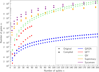
Fig. 18: The overall gate counts of the five algorithms QAOA (blue), QFT (red), QV (green), Supremacy (orange), and Sycamore (purple) depending on different numbers of qubits. For each algorithm, the gate counts of the original (triangles) and compiled (circles) circuits are depicted. For the latter, the rebasing approach with the lowest gate count is used.

As depicted in Fig. 18, the compiled circuits of QAOA, QFT, and QV have higher overall gate counts compared to the original circuits. While for QAOA and QV the two-qubit gate counts remained the same or decreased, for QFT the two-qubit gate counts at most doubled during compilation. This is because the original circuits contain CPhase gates as two-qubit gates, each of which was decomposed into two ZZ gates. However, some of the ZZ gates became redundant and could be removed after commuting the single-qubit gates through them. For Supremacy and Sycamore, the overall gate counts in the compiled circuits are lower than in the original circuits. Here, the circuits contain several T and Z gates, which phase tracking removed. The two-qubit CZ gates of the original circuits were replaced by one ZZ and two Rz gates where phase tracking could also remove the latter. However, for 69 % of the circuits, the two-qubit gate counts increased slightly due to the block commutation with correction unitaries, while the single-qubit gate counts are up to 2.20 times lower. For all five algorithms, the number of qubits has no effect on the gate count relation.

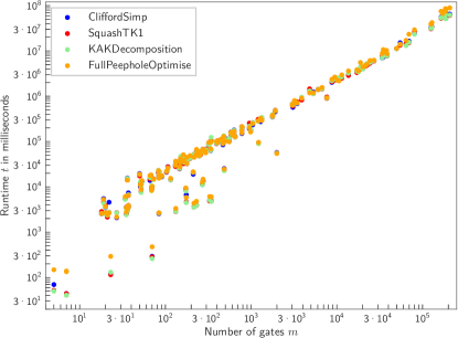
(a) Runtimes of our complete compilation flow. All four compilation approaches behave nonlinearly with the number of gates.

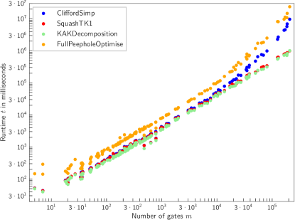
(b) Runtimes of our compiler when executed without the block commutation with correction unitaries. In this case, the CliffordSimp and FullPeepholeOptimise approaches lead to a nonlinear scaling of the runtimes, while the SquashTK1 and KAKDecomposition approaches behave linearly with the number of gates.

Fig. 19: Runtimes of our compiler for the different rebasing approaches depending on the number of gates. Each color represents one of the rebasing approaches: CliffordSimp (dark blue), SquashTK1 (red), KAKDecomposition (green), and FullPeepholeOptimise (orange). Each dot represents one of the 153 circuits in the circuit library.

The runtimes of the four approaches versus the number of gates in the original circuits for the circuit library are shown in 19(a). All four approaches had nonlinear compile times. While the compile times of the CliffordSimp, SquashTK1, and KAKDecomposition approaches were nearly the same for the different circuits, the compile time of the FullPeepholeOptimise approach was on average 1.11 times higher. The standard deviation for all four approaches was on average about 6.53 % of the average runtimes. The evaluation of the runtimes for the five algorithms showed the same runtime behavior without any influence of the number of qubits.

Compiling the circuits without the block commutation with correction unitaries achieved the compile times depicted in 19(b). For small circuits, the SquashTK1 and KAKDecomposition approaches resulted in compile times of about 4 ms per gate of the original circuits. In contrast, the CliffordSimp and FullPeepholeOptimise approaches showed a nonlinear growth of the compile times with the number of gates of the original circuits, with the FullPeepholeOptimise approach having on average 2.09 times higher compile times than the CliffordSimp approach. The reasons for the nonlinear growth are the additional optimizations executed by Pytket’s CliffordSimp and FullPeepholeOptimise passes, which led to nonlinear runtime scaling. As mentioned in Sec. 4.10.2, the block commutation with correction unitaries has a nonlinear runtime because it is applied to the blocks recursively. This also led to nonlinear compile times of the SquashTK1 and KAKDecomposition approaches in the cases where the block commutation with correction unitaries was executed. In contrast, the other transformations executed in the SquashTK1 and KAKDecomposition approaches only iterate a constant number of times over each gate, resulting in linear runtimes of these two approaches when the block commutation with correction unitaries was not applied.

The factors of the compile time increases when executing the block commutation with correction unitaries compared to the compilation without the block commutation with correction unitaries are shown in Fig. 20. On average, the runtimes with the block commutation with correction unitaries were 53.75 times higher for the KAKDecomposition approach, followed by the SquashTK1 approach with 48.92 times, the CliffordSimp approach with 41.49 times, and the FullPeepholeOptimse approach with 21.45 times. While the factors for the SquashTK1 and KAKDecomposition approaches are approximately constant in a certain range, the factors for the CliffordSimp and FullPeepholeOptimise approaches are approximately constant up to a circuit size of 10,000 gates, and decrease for higher number of gates.

In the following, we compare the impact of the different compilation stages on the results of the circuits. To compare the gate counts, for each circuit we used the approach (CliffordSimp, SquashTK1, KAKDecomposition, or FullPeepholeOptimise) which produced the lowest overall gate count after executing our entire compiler flow as the baseline in all evaluations. If more than one approach had the same overall gate count, we preferred the result with the lowest two-qubit gate count. The impact of the different compilation stages are depicted in 21(a) for the circuit library and in 21(b) for the five algorithms.

As a naive compilation, the gates of the original circuit were replaced using Pytket’s RebaseCustom pass as described in Sec. 4.4 and the ZZ decomposition given in (9) and (29). Afterwards, the circuit was transformed into our trapped-ion native gate set $\mathcal{N}$. Comparing this naive transformation with our compiler for the circuit library, the resulting circuits from our compiler have 2.50 to 5.38 times fewer single-qubit gates and up to 1.38 times fewer two-qubit gates. However, for 33 % of the circuits, our compiler produced results with up to 1.27 times more two-qubit gates. This is due to the additional gates inserted during the block commutation with correction unitaries to reduce the amount of shuttling operations. On average, our compiler produced circuits with 3.29 times fewer overall gates. For the evaluated circuits, this naive transformation produced results with about 1.10 times lower single-qubit gate counts when the Ry was not excluded from the native gate set before executing the RebaseCustom pass. This is because the naive transformation need not take care of commutations, and including Ry gates allows the gates to be replaced by shorter gate sequences.

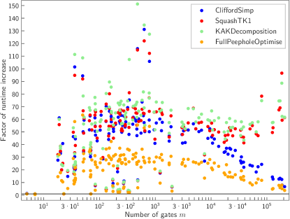
Fig. 20: The runtime increases of our complete compilation flow compared to our compiler when executed without the block commutation with correction unitaries for the different rebasing approaches CliffordSimp (dark blue), SquashTK1 (red), KAKDecomposition (green), and FullPeepholeOptimise (orange) depending on the number of gates. Each dot represents one of the 153 circuits in the circuit library. For all circuits with an increase factor greater than one (the horizontal black line), our complete compilation flow has a longer runtime than our compiler when executed without the block commutation with correction unitaries.

Comparing the naive compilation with our compiler for the five algorithms shows that for QAOA and QV, the overall and single-qubit gate count reduction factors first decrease as the number of qubits increases. Then the overall gate count reduction factors converge to 3.13 for QAOA and 5.39 for QV, while the single-qubit gate count reduction factors converge to 3.43 for QAOA and 6.48 for QV. While the overall gate count reduction factors for Supremacy and Sycamore increase only slightly, the single-qubit gate count reduction factors increase from 9.85 to 11.16 for Supremacy and from 9.92 to 11.13 for Sycamore as the number of qubits increases. The reason for these large increases is that the substitution of the CZ gates contained in the circuits used by the naive compilation requires 15 single-qubit gates, while our compiler requires only two single-qubit gates for a CZ decomposition. Moreover, our compiler can remove the z-rotations contained in the circuit using phase tracking. While for QAOA, Supremacy, and Sycamore the gate count reduction factors for two-qubit gates are around one, meaning that the circuits calculated by our compiler have approximately as many two-qubit gates as the naive compilation, for QV the reduction factor decreases from 1.25 to a factor slightly above one. For QFT, the gate count reduction factors also increase with the number of qubits. While our compiler required 4.46 times fewer single-qubit gates and the same number of two-qubit gates compared to the naive compilation for five qubits, our compiler required 5.94 times fewer single-qubit gates and 1.27 times fewer two-qubit gates for 49 qubits. For all five algorithms, our compiler generated lower single-qubit gate counts when the Ry was not excluded from the native gate set before the RebaseCustom pass was executed. In this case, the single-qubit gate counts are on average 1.04 times lower for QAOA and QV, 1.10 times lower for QFT, 1.14 times lower for Supremacy, and 1.16 times lower for Sycamore compared to a compilation without Ry as a native gate. The higher factors for Supremacy and Sycamore are due to the fact that these circuits already contain several Ry gates, which do not need to be replaced when the Ry gate is added to the native gate set.

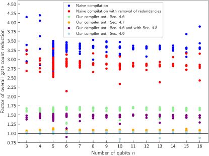
(a) The overall gate count reductions for the 153 circuits in the circuit library. The circuits are sorted by the number of qubits used.

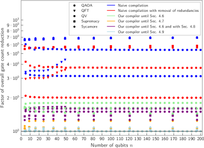
(b) The overall gate count reductions for the algorithms QAOA (circles), QFT (triangles), QV (crosses), Supremacy (squares), and Sycamore (pluses) depending on different numbers of qubits.

Fig. 21: The overall gate count reductions of our complete compilation flow compared to the following less optimized compilations: (1) a naive compilation which replaces gates only with respect to our trapped-ion native gate set $\mathcal{N}$, but without any optimization (dark blue dots), (2) the naive compilation with additional removal of trivial redundancies (red dots), (3) the compilation as depicted in Fig. 3, but only up to the transformation described in Sec. 4.6 (green dots), (4) the compilation up to phase tracking (orange dots), (5) the compilation up to block aggregation but without phase tracking (purple dots), and (6) the compilation up to the commutation of blocks and blockless sequences on disjoint sets of qubits (light blue dots). For each circuit, the best compilation result of the four different rebasing approaches is used. For all circuits with a reduction factor greater than one (the horizontal black line), our complete compilation flow produces a circuit with a lower gate count than the less optimized compilations.

Comparing our compiler to the naive approach, but additionally removing trivial redundancies using Pytket’s RemoveRedundancies pass, the compiled circuits in the circuit library have between 2.50 and 4.29 times fewer single-qubit gates and up to 1.13 times fewer two-qubit gates. For the same reason as for the naive approach, our compiler produced results with up to 1.27 times more two-qubit gates for 34 % of the circuits. The overall gate counts of our compiler are on average 2.86 times lower than the overall gate counts of the improved naive transformation. These high factors show the potential of the optimizations applied by our compiler. In the improved naive transformation, for 98 % of the circuits our compiler calculated results with a lower or equal gate count when the Ry gate was excluded from the native gate set before executing the RebaseCustom pass. This is because excluding gates from the native gate set reduces the number of different gates. Consequently, gates of the same type are more likely to be located next to each other, allowing for better redundancy removal.

The comparison of the advanced naive compilation for QAOA, QFT, QV, and Supremacy shows the same trends as the naive compilation with lower gate count reduction factors. E. g., the overall gate count reduction factors converge to 2.00 for QAOA and 3.72 for QV as the number of qubits increases. The only exception is Sycamore, whose overall gate count reduction factor is 5.83 for four qubits and converges to 5.64 for a higher number of qubits. While the overall gate count reduction factor decreases with the number of qubits, the single-qubit gate count reduction factor increases from 8.47 to 8.89, and the two-qubit gate count reduction factors are around one as in the naive compilation. For all algorithms except QAOA, the improved naive compilation produced better results when the Ry gate was excluded from the native gate set before executing the RebaseCustom pass for the reason mentioned above. For QAOA, the results of the improved naive compilation have about 1.06 times fewer single-qubit gates when including the Ry gate. The reason for this is that the circuits benefit more from the shorter CNOT decomposition

$$\texttt{CNOT}_{i,j}= \hskip 2.84526pt\texttt{Ry}_{j}\left(\tfrac{\pi}{2}\right)\texttt{Rx}_{j}\left(\pi\right)\texttt{Rx}_{i}\left(\pi\right)\texttt{ZZ}_{i,j}\left(\tfrac{\pi}{2}\right)\texttt{Ry}_{j}\left(\tfrac{\pi}{2}\right)$$

$$\cdot \hskip 2.84526pt\texttt{Rx}_{j}\left(\tfrac{\pi}{2}\right)\texttt{Ry}_{i}\left(\tfrac{\pi}{2}\right)\texttt{Rx}_{i}\left(\tfrac{\pi}{2}\right)\texttt{Ry}_{i}\left(\tfrac{\pi}{2}\right)$$ (30)

which can be used when including the Ry gate than from the additional redundancy removal possible when excluding the Ry gate.

For the next evaluation, our compiler was executed as depicted in Fig. 3, but skipping phase tracking, block aggregation, and the block commutation with correction unitaries. Comparing our entire compiler flow with the flow skipping these three optimizations for the circuit library, our entire compiler calculated circuits with 1.38 to 2.05 times fewer single-qubit gates. For 47 % of the circuits, our entire compiler produced results with up to 1.27 times more two-qubit gates. Since phase tracking and block aggregation do not change the two-qubit gates, the block commutation with correction unitaries inserted the additional two-qubit gates to reduce the amount of shuttling operations. The overall gate counts of our entire compiler flow are on average 1.65 times lower than those of the reduced compiler.

For QAOA, the single-qubit reduction factors remain constant at 1.71 independently of the number of qubits. In contrast, for QFT and QV, the single-qubit gate count reduction factors increase with the number of qubits from 1.80 to 1.97 for QFT and from 1.94 to 2.00 for QV, while the factors decrease from 1.97 to 1.75 for Supremacy and from 2.05 to 2.01 for Sycamore. The overall gate count reduction factors are similar to those for single-qubit gates, but with smaller factors. For all algorithms except Sycamore, the amount of two-qubit gates for the compilation without phase tracking, block aggregation, and the block commutation with correction unitaries is as large as the amount of our entire compilation flow. Only for Sycamore, our entire compiler flow has a slightly higher two-qubit gate count than the compilation without the skipped optimizations.

In the following, phase tracking was also executed, but block aggregation and the block commutation with correction unitaries were not executed. In this case, for the circuit library, the overall gate counts of our entire compilation flow are on average only 1.07 times and the single-qubit gate counts are up to 1.20 times lower than the gate counts of the flow without block aggregation and the block commutation with correction unitaries. For the ising_model circuits, the single-qubit gate counts of our entire compiler flow are up to 1.15 times higher. The reason for this is that these circuits contain several Rz gates, which phase tracking removed. However, the block commutation with correction unitaries introduced new gates to reduce shuttling operations.

Using this reduced compilation flow for QAOA and QV, the gate counts are exactly the same as for our entire compiler flow. This means that block aggregation and the block commutation with correction unitaries do not affect the gate counts of these circuits when executing the transformations after phase tracking. For QFT, the single-qubit gate count reduction factor is 1.02 for five qubits and decreases to one for 30 and more qubits. While for Supremacy the single-qubit gate count reduction factor decreases from 1.15 to 1.10 as the number of qubits increases, for Sycamore the single-qubit gate count reduction factor starts at 1.17 for the four-qubit circuit and converges to a factor of 1.41.

Compared to the compiler which did not perform phase tracking and the block commutation with correction unitaries, but performed block aggregation, the overall gate counts of our entire compiler flow for the circuit library are on average 1.45 times lower, and the single-qubit gate counts are up to 1.77 times lower. Since the reduction factors are higher than in the previous case of executing phase tracking instead of block aggregation, the impact of block aggregation is less than the impact of phase tracking. However, an exception is the circuit graycode6_47, which has a lower single-qubit gate count when not using phase tracking and the block commutation with correction unitaries. The reason for this is the construction of this circuit, which consists only of CNOT gates. Consequently, this circuit directly benefits from the symmetric structure of the CNOT decomposition in (10), which favors block aggregations.

For QAOA, the single-qubit gate counts of our entire compiler are about 1.57 times lower than the counts of the compilation without phase tracking and the block commutation with correction unitaries. However, these factors grow from 1.76 to 1.97 for QFT, from 1.72 to 1.75 for QV, and from 1.57 to 1.66 for Supremacy as the number of qubits increases. Only for Sycamore, they decrease slightly from 1.48 to 1.46. For QFT, the single-qubit gate counts are the same as in the compilation even without block aggregation, except for the five-qubit circuit. This shows that QFT does not benefit from block aggregation when executed without prior phase tracking. On the other hand, since the reduction factors for QAOA, QV, Supremacy, and Sycamore are lower than in the compilation even without block aggregation, these algorithms benefit from block aggregation in this case. However, because the reduction factors are higher than in the previous case of executing phase tracking instead of block aggregation, the impact of block aggregation is less pronounced than the impact of phase tracking.

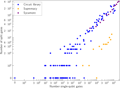
Fig. 22: Number of splits performed during angle splitting in Sec. 4.8.2, depending on the number of single-qubit gates in the original circuit. For each circuit, the best compilation result of the four different rebasing approaches is used. Each dark blue dot represents at least one circuit in the circuit library, with splits applied to 97 of the 153 circuits. While angle splitting was performed on every circuit of Sycamore (purple dots), it was not applied to the 25-qubit circuit of Supremacy (orange dots). Since angle splitting was not performed on any circuit of QAOA, QFT, and QV, these circuits are not depicted.

Evaluating the angle splitting in Sec. 4.8.2 shows that our compiler applied this technique to 63 % of the circuits in the circuit library. On these circuits, our compiler performed angle splitting on 0.08 % to 4.65 % and on average on 0.72 % of the single-qubit gates in the original circuits. Of the five algorithms, only Supremacy and Sycamore benefit from angle splitting. The number of single-qubit gates of the original circuit which were split by angle splitting is shown in Fig. 22. This number tends to grow with the number of single-qubit gates.

As a final case, we compare our entire compiler flow to the flow without the block commutation with correction unitaries. For the circuit library, our entire compilation flow has on average 1.02 times lower overall gate counts and up to 1.09 times lower single-qubit gate counts than the compilation without the block commutation with correction unitaries. The three ising_model circuits and the circuit decod24-v0_38 have up to 1.15 times lower single-qubit gate counts when not executing the block commutation with correction unitaries. As mentioned above for 47 % of the circuits, performing the block commutation with correction unitaries results in up to 1.27 times higher two-qubit gate counts. The increase in the gate counts is due to the additional gates inserted during the block commutation with correction unitaries. However, the next subsection shows that the insertion of these additional gates results in a reduction of shuttling operations. Although 47 % of the circuits have a higher two-qubit gate count, only 3 % of the circuits have a higher overall gate count after executing the block commutation with correction unitaries, showing its potential to reduce single-qubit gates.

Compiling the circuits of the five algorithms without the block commutation with correction unitaries produced exactly the same results for QAOA, QFT, and QV as compiling even without block aggregation. Consequently, block aggregation has no effect on these three algorithms when executed after phase tracking. Additionally, as mentioned above, the block commutation with correction unitaries has no effect on the circuits of QAOA and QV, since the compilation without the block commutation with correction unitaries produced the same results as our entire compiler flow. However, the single-qubit gate count reduction factor for QFT decreases from 1.02 for the five-qubit circuit to one for the circuits with 30 and more qubits. This shows that for QFT, the block commutation with correction unitaries slightly reduces the single-qubit gate counts for the circuits up to 25 qubits. The single-qubit gates of our entire compiler flow are about 1.04 times less for Supremacy and 1.14 times less for Sycamore, independent of the number of qubits, than for the compilation without the block commutation with correction unitaries. Only for Sycamore, our entire compiler flow has a slightly higher number of two-qubit gates compared to the compilation without the block commutation with correction unitaries. This means that the block commutation with correction unitaries inserted some two-qubit gates to reduce the amount of shuttling operations.

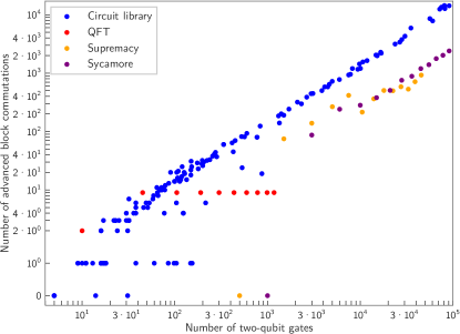
Fig. 23: Number of block commutations with correction unitaries applied, depending on the number of two-qubit gates in the original circuit. For each circuit, the best compilation result of the four different rebasing approaches is used. Each dark blue dot represents at least one circuit in the circuit library where the block commutation with correction unitaries was performed on 148 of the 153 circuits. While the block commutation with correction unitaries was applied to every circuit of QFT (red dots), it was not performed on the smallest circuit of Supremacy (orange dots) and Sycamore (purple dots). Since the block commutation with correction unitaries was not applied to any circuit of QAOA and QV, these circuits are not depicted.

Evaluating the number of commutations executed, we found that our compiler applied commutations to 97 % of the circuits in the circuit library. Up to 14,345 commutations were executed on these circuits. The number of executed commutations ranges from 0.65 % to 21.88 % and averages out to 12.28 % of the number of two-qubit gates in the original circuits. For the five algorithms, our compiler only executed commutations on the circuits of QFT, Supremacy, and Sycamore. While the number of commutations grows with the number of two-qubit gates for the circuits in the circuit library, Supremacy, and Sycamore, for QFT our compiler executed two commutations on the five-qubit circuit and applied nine commutations constantly to the circuits with a higher number of qubits. The number of commutations depending on the number of two-qubit gates in depicted in Fig. 23.

6.2 Impact on the shuttling

In the following, we analyze the impact of the commutation of blocks and blockless sequences on disjoint sets of qubits and of the block commutation with correction unitaries on the shuttling by comparing the required number of translate, separation/merge, and physical ion swap operations. Therefore, we arranged as many ions in a linear chain as the circuit to be compiled has qubits. The chain was modeled as a linear graph with each vertex representing an ion. To map the logical qubits of the circuit to the ions, we used two different Pytket passes, the GraphPlacement pass and the LinePlacement pass, which use different heuristics. For each circuit, we executed both passes and obtained a mapping for each pass. Afterwards, we used Pytket’s RoutingPass on both mappings, which inserts SWAP gates so that two-qubit gates are only executed on ions whose vertices are adjacent. The Shuttling Compiler executed all SWAP gates inserted by Pytket as physical ion swaps. Due to the two mappings, we got two results, from which we selected the result with the lower number of SWAP gates for submission to the Shuttling Compiler [10].

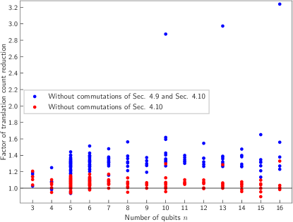
(a) The translation count reductions for the 153 circuits in the circuit library. The circuits are sorted by the number of qubits used.

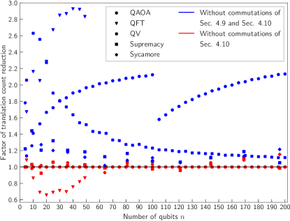
(b) The translation count reductions for the algorithms QAOA (circles), QFT (triangles), QV (crosses), Supremacy (squares), and Sycamore (pluses) depending on different numbers of qubits.

Fig. 24: The translation count reductions of our complete compilation flow compared to (1) the compilation without the commutation of blocks and blockless sequences on disjoint sets of qubits as well as without the block commutation with correction unitaries (blue dots) and (2) only without the block commutation with correction unitaries (red dots). For each circuit, the translations for the best compilation result of the four different rebasing approaches were calculated. For all circuits with a reduction factor greater than one (the horizontal black line), our complete compilation flow produces a circuit with a lower translation count than the less commuted compilation flows.

When both types of commutations were executed, 97 % of the circuits in the circuit library required fewer or the same number of translations as when both types of commutations were not executed. The commutations reduced the number of translations by factors up to 3.24, and on average by a factor of 1.33. Compared to a compiler which executed the commutation of blocks and blockless sequences on disjoint sets of qubits, but not the block commutation with correction unitaries, our compiler calculated results which lead to up to 1.33 times and on average 1.06 times fewer translations for 89 % of the circuits. The impact of the commutations on the amount of translations for the circuits in the circuit library is depicted in 24(a). The differences in the factors show that the commutation of blocks and blockless sequences on disjoint sets of qubits has a higher impact on the translation counts. However, the commutation of blocks and blockless sequences on disjoint sets of qubits has no effect on the amount of separation/merge and ion swap operations. Using the block commutation with correction unitaries also reduced the amount of separation/merge operations for 94 % of the circuits by factors up to 1.20 and on average by 1.04. Additionally, it reduced the number of ion swaps for 97 % of the circuits by factors up to 1.67 and on average by 1.12.

The impact of both types of commutations on the five algorithms is shown in 24(b). As mentioned in the last subsection, the compiler did not execute the block commutation with correction unitaries on the circuits of QAOA and QV. Moreover, as for the circuit library, the commutation of blocks and blockless sequences on disjoint sets of qubits did not affect the amount of separation/merge and ion swap operations for all five circuits. Consequently, for QAOA and QV, only the impact of the commutation of blocks and blockless sequences on disjoint sets of qubits on the translation count needs to be considered. For QV, the result of our entire compiler flow requires 2.63 times fewer translations for ten qubits compared to a compilation without the commutation of blocks and blockless sequences on disjoint sets of qubits. This translation count reduction factor decreases to 1.11 for 200 qubits. In contrast, for QAOA, the translation count reduction factor is 1.13 for five qubits and increases to 2.12 for 100 qubits. From there, it decreases rapidly to 1.58 for 105 qubits and increases again to 2.13 for 200 qubits. The reason for the rapid decrease is Pytket’s placement pass, which we used to map the logical qubits to ions. The qubits in the QAOA algorithm have a nearest neighbor interaction. This means that the qubit $q_{0}$ interacts only with the qubit $q_{1}$, the qubit $q_{n-1}$ only with the qubit $q_{n-2}$, and all other qubits $q_{i}$ only with the qubits $q_{i-1}$ and $q_{i+1}$. This allows to map the logical qubits to the ion chain in ascending order. I. e., $q_{0}$ is mapped to the leftmost ion of the ion chain, $q_{1}$ is mapped to the ion next to $q_{0}$ on the right, and so on until $q_{n-1}$ is mapped to the rightmost ion of the chain. Up to the 100-qubit circuit, Pytket’s placement pass could map the logical qubits exactly according to this scheme. However, when the circuits used more than 100 qubits, the placement pass mapped $q_{n-1}$ to the leftmost ion, $q_{n-2}$ to the ion next to $q_{n-1}$ on the right, and so on until the qubit $q_{100}$ was mapped. To the ion to the right of $q_{100}$ it mapped the qubit $q_{0}$, and from there it mapped all the qubits in ascending order to the ions until it reached the qubit $q_{99}$. Since $q_{99}$ also interacts with $q_{100}$, which the placement pass mapped 100 ions to the left, $q_{99}$ had to be swapped with 99 intermediate ions to execute the gate with $q_{100}$. The placement pass placed the ions according to this scheme, regardless of whether commutations had been used. While the additional ion swap and separation/merge operations did not affect the reduction factors of these operations, the additional translations resulted in a decreasing translation count reduction factor between the 100- and 105-qubit circuits.

For QFT, our entire compilation required between 1.67 and 2.93 times fewer translations than the compilation without both types of commutations. When executing the commutation of blocks and blockless sequences on disjoint sets of qubits, but not the block commutation with correction unitaries, the compiler required up to 1.52 times fewer translations and up to 1.22 times fewer seperation/merge operations for the circuits with 10 and more qubits compared to our entire compilation flow. Moreover, the number of ion swaps is up to 1.64 times higher for our entire compilation flow.

Furthermore, for both Supremacy and Sycamore, our entire compiler flow calculated circuits requiring fewer translations than a compilation without both types of commutations. For Supremacy, our entire compiler required between 1.05 and 1.44 times fewer translations, while for Sycamore it required between 1.02 and 1.78 times fewer. In this range, the factors alternate between the different numbers of qubits. When we compare our entire compiler flow with a compiler which used the commutation of blocks and blockless sequences on disjoint sets of qubits, but not the block commutation with correction unitaries, our compiler generated results with a lower number of translations for 54 % of the Supremacy circuits and 77 % of the Sycamore circuits. Thus, our entire compiler calculated results with up to 1.11 times fewer and up to 1.08 times more translations for Supremacy, and with up to 1.15 times fewer and up to 1.07 times more translations for Sycamore. For both algorithms, the factors alternate between the different numbers of qubits in these ranges. Regarding the amount of separation/merge and ion swap operations, our entire compiler flow calculated results with fewer separation/merge and ion swap operations for half of the circuits of Supremacy and Sycamore. While the reduction factors for separation/merge range from 0.95 to 1.08 for Supremacy and from 0.96 to 1.03 for Sycamore, the reduction factors for ion swap range from 0.93 to 1.09 for Supremacy and from 0.95 to 1.04 for Sycamore. For all circuits where our entire compiler flow produced a result with a lower number of separations/merge operations, the result also has a lower number of ion swaps. The same applies to the case where our entire compiler flow calculated a result with a higher number of separations/merge and ion swap operations.

6.3 Comparison to other compilers

We benchmarked our compiler against built-in Pytket passes, first using its FullPeepholeOptimise pass. Then we rebased the circuits to $\left\{\texttt{Rx},\texttt{Rz},\texttt{ZZ}\right\}$ using Pytket’s RebaseCustom pass with the TK1 decomposition in (8a) and the CNOT decomposition in (10). There are exceptions for the circuits graycode6_47, ex1_226, and xor5_254, as well as all QAOA circuits and Sycamore circuits with nine and more qubits, which we rebased to $\left\{\texttt{Rx},\texttt{Ry},\texttt{Rz},\texttt{ZZ}\right\}$ because Pytket calculated significantly better results for these circuits with Ry gate than without Ry gate. After rebasing, we applied the repeated removal and commutation of gates based on Pytket’s built-in procedures from Sec. 4.2. Since Pytket does not allow the gates of the native gate set to be constrained to certain angles, it cannot directly transform the gates to our trapped-ion native gate set $\mathcal{N}$. To make the gate counts comparable, we applied the transformation from Sec. 4.6 to the circuits.

For the Qiskit compilation, we first applied the ZZ decomposition given in (9) and (29) to the circuits, because Qiskit cannot transform ZZ gates with $\theta\neq\tfrac{\pi}{2}$ already in the circuits into ZZ gates with $\theta=\tfrac{\pi}{2}$ and a set of single-qubit gates. Afterwards, we applied Qiskit’s BasisTranslator pass with the target basis $\left\{\texttt{Rx},\texttt{Ry},\texttt{Rz},\texttt{ZZ}\right\}$. The only exceptions are the circuits graycode6_47, ex1_226, and xor5_254, for which the Ry gate was removed from the target basis because Qiskit calculated better results for these circuits without Ry gate than with Ry gate. After rebasing, we executed the transpile function of the Qiskit compiler module with optimization level three. Like Pytket, Qiskit cannot transform the gates to our trapped-ion native gate set $\mathcal{N}$, so we used Sec. 4.6 to get comparable gate counts.

The gate count reductions achieved by our compiler compared to Pytket and Qiskit are summarized in 25(a) for the circuit library and in 25(b) for the five algorithms.

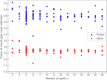
(a) The overall gate count reductions for the 153 circuits in the circuit library. The circuits are sorted by the number of qubits used.

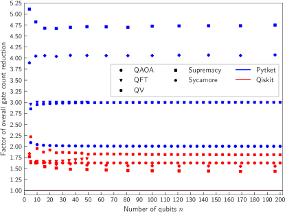
(b) The overall gate count reductions for the algorithms QAOA (circles), QFT (triangles), QV (crosses), Supremacy (squares), and Sycamore (pluses) depending on different numbers of qubits.

Fig. 25: The overall gate count reductions of our compiler compared to Pytket (dark blue dots) and Qiskit (red dots) standard passes. As result for our compiler, the compilation result with the lowest gate count of the four different rebasing approaches is used for each circuit. For all circuits with a reduction factor greater than one (the horizontal black line), our compiler produces a circuit with a lower gate count than either Pytket or Qiskit.

Compared to standard Pytket, our compiler always computed results with lower gate counts. For the circuit library, there are between 2.14 and 3.24 times fewer gates. A more detailed examination shows that for all circuits our compiler produced results with 2.50 to 4.20 times fewer single-qubit gates, while the two-qubit gate counts are only up to 1.08 times less or equal for 51 % of the circuits. The main reason for the small fraction of less or equal two-qubit gate counts is the block commutation with correction unitaries, which added additional two-qubit gates to the circuit to reduce shuttling operations. Without the block commutation with correction unitaries, our compiler calculated results with fewer two-qubit gates for 84 % of the circuits.

For QAOA, our compiler required between 2.23 and 2.14 times fewer single-qubit gates than Pytket, with the factor decreasing as the number of qubits increases. In contrast, the reduction factors increase with the number of qubits from 3.80 to 3.99 for QFT and from 3.26 to 3.50 for QV. For all three algorithms, the results of our compiler have as many two-qubit gates as Pytket’s results, independently of the number of qubits. The single-qubit gate count reduction factor for Supremacy increases from 7.02 for 16 qubits to 7.42 for 196 qubits. For Sycamore, our compiler calculated circuits with 5.49 to 6.20 times fewer single-qubit gates than Pytket, with the factor increasing with the number of qubits. The two-qubit gate count reduction factors for both algorithms are the same as for the naive compilation in Sec. 6.1, showing that Pytket calculated the same amount of two-qubit gates. Thus, for the Sycamore circuits and half of the Supremacy circuits, Pytket produced results with slightly lower two-qubit gate counts. Again, the reason for the higher two-qubit gate counts of our compiler is the block commutation with correction unitaries. Without it, the two-qubit gate counts of our compiler and Pytket are the same for all five algorithms, independently of the number of qubits.

The main reason for Pytket’s higher single-qubit gate counts is that it cannot apply phase tracking. Due to this limitation, the circuits contain several Rz gates, which in our compilation flow can only appear at the end of the circuit. Additionally, the Rz gates are often sandwiched by Rx gates, which prevents the Rx gates from being merged and removed when their angle is $\theta=0$. Since we had to execute all four approaches of our compiler to find the best result, and since one of our approaches also includes Pytket’s FullPeepholeOptimise pass, the runtimes of our compiler were always worse than Pytket’s runtimes.

The comparison with standard Qiskit shows for the circuit library that our compilation leads to 1.27 to 2.00 times fewer gates. Furthermore, the number of single-qubit gates is between 1.40 and 2.34 times less for our compiler, and the number of two-qubit gates is between 0.79 and 1.25 times less, with our compiler requiring a higher number of two-qubit gates for 33 % of the circuits. As in the Pytket comparison, the reason for the higher number of two-qubit gates is the block commutation with correction unitaries. Without executing it, our compiler needed fewer two-qubit gates for all circuits with reduction factors up to 1.25.

For QAOA, our compiler calculated circuits with 1.71 times fewer single-qubit gates and the same number of two-qubit gates compared to Qiskit, independently of the number of qubits. In contrast, for QFT, the single-qubit gate count reduction factor increases from 1.93 to 2.01 with the number of qubits. Regarding the amount of two-qubit gates, our compiler and Qiskit produced results with the same number of two-qubit gates for the circuits up to 25 qubits, while for 30 and more qubits the results of our compiler have between 1.01 and 1.14 times fewer two-qubit gates, with the factor increasing with the number of qubits. For the other three algorithms, the single-qubit gate count reduction factors decrease from 2.43 to 2.01 for QV, from 2.21 to 1.74 for Supremacy, and from 2.29 to 1.94 for Sycamore as the number of qubits increases. The two-qubit gate count reduction factors for all three algorithms are the same as for the naive compilation comparison in Sec. 6.1. Thus, Qiskit’s results have the same number of two-qubit gates as the naive approach. This means that for QV, the amount of two-qubit gates of our compiler is between 1.01 and 1.25 times lower than Qiskit’s, with a decreasing factor as the number of qubits increases. Moreover, for Supremacy and Sycamore, Qiskit’s results have exactly the same number of two-qubit gates as Pytket. This means that for the Sycamore circuits and half of the Supremacy circuits, Qiskit produced results with slightly lower two-qubit gate counts for the same reason mentioned above.

The main reason for the single-qubit gate count reductions achieved by our compiler is the same as for Pytket. Regarding the runtime, Qiskit was always faster than our compiler. However, Qiskit’s faster runtime comes at the cost of a larger number of gates.

In summary, our compiler achieved larger reductions compared to Pytket, with an average reduction factor of 2.80 for the circuit library, while the average reduction factor compared to Qiskit is only 1.67. Compared to both standard passes, our compiler always computed circuits with lower overall and single-qubit gate counts.

7 Conclusion and outlook

We have presented a quantum circuit compiler for a shuttling-based ion trap quantum computer that implements a number of optimization techniques such as phase tracking, block aggregation, and a block commutation with correction unitaries. These reduce the number of gates and shuttling operations when compiling a quantum circuit into the native gate set. Compared to other compilation algorithms, our compiler reduces the gate counts by factors of up to 5.11 for Pytket and up to 2.22 for Qiskit.

In the future, we plan to extend the functionality of our compiler, increase its performance using more advanced compilation techniques, and adapt it to more powerful architectures. The next architectural step will be to adapt it to a platform which allows simultaneous addressed manipulation of larger subsets of commonly confined trapped-ion qubits, where gates can be executed in parallel. This will allow low-resource quantum computation on sub-registers, interleaved with time-consuming register reconfiguration steps. Future multiplexed laser addressing units [53] will also allow the execution of multi-qubit gates, so that e. g., three-qubit Toffoli gates can be realized within a single laser interaction sequence [54] instead of being decomposed into two-qubit gates. This can massively increase the quantum computational power of a trapped-ion platform, but also requires an advanced compilation layer.

8 Acknowledgements

We acknowledge funding by the German Federal Ministry of Education and Research (BMBF) via the VDI within the projects HFAK and IQuAn. The research is based upon work supported by the Office of the Director of National Intelligence (ODNI), Intelligence Advanced Research Projects Activity (IARPA), via the U.S. Army Research Office grant W911NF-16-1-0070. The views and conclusions contained herein are those of the authors and should not be interpreted as necessarily representing the official policies or endorsements, either expressed or implied, of the ODNI, IARPA, or the U.S. Government. The U.S. Government is authorized to reproduce and distribute reprints for Governmental purposes notwithstanding any copyright annotation thereon. Any opinions, findings, and conclusions or recommendations expressed in this material are those of the author(s) and do not necessarily reflect the view of the U.S. Army Research Office.

Appendix A Detailed evaluation results

This appendix presents the detailed results of the evaluations described in Sec. 6.1 and Sec. 6.3. For the 153 quantum circuits in the circuit library, Tab. 1 shows the results for the circuits with three to five qubits, and Tab. 2 shows the results for the circuits with six to sixteen qubits. We took all these circuits from [47]. For QAOA, QFT, and QV, Tab. 3 shows the results for various numbers of qubits, while Tab. 4 shows the results for Supremacy and Sycamore. While we generated the circuits for QAOA, QFT, Supremacy, and Sycamore using the quantum circuit generator from [52], we generated the QV circuits using Qiskit [17].

Tab. 1: Results of the evaluations for the circuits in the circuit library with three to five qubits. The first column shows the name, number of qubits (q), single-qubit gate count (1qg), and two-qubit gate count (2qg) of the original circuit. The next four columns show the single-qubit and two-qubit gate counts for our CliffordSimp, SquashTK1, KAKDecomposition, and FullPeepholeOptimise approaches. The green markers show which approaches have the lowest single-qubit and two-qubit gate counts for each circuit. If multiple approaches have the same single-qubit or two-qubit gate count, the approach with the lowest overall gate count is marked. The last two columns show the results of the standard Pytket and Qiskit passes. In each of these columns, the first two entries show the single-qubit and two-qubit gate counts. The last entry in each column shows the factors by which the best approach of our compiler reduces the overall gate count compared to Pytket or Qiskit (rg).

Original Circuit				CliffordSimp		SquashTK1		KAK		FullPeephole			Pytket			Qiskit
Name	q	1qg	2qg	1qg	2qg	1qg	2qg	1qg	2qg	1qg	2qg		1qg	2qg	rg	1qg	2qg	rg
ex-1_166	3	10	9	20	8	22	9	22	9	20	8		76	8	3.00	40	9	1.75
ham3_102	3	9	11	19	8	18	9	18	9	19	8		74	8	3.04	44	10	2.00
3_17_13	3	19	17	44	17	44	17	44	17	44	17		143	17	2.62	81	17	1.61
miller_11	3	27	23	54	22	53	23	53	23	61	19		227	19	3.24	100	23	1.62
4gt11_84	4	9	9	24	9	24	9	24	9	24	9		80	9	2.70	47	9	1.70
rd32-v0_66	4	18	16	30	12	30	12	30	12	30	12		105	12	2.79	69	14	1.98
rd32-v1_68	4	20	16	29	12	29	12	29	12	29	12		105	12	2.85	68	14	2.00
decod24-v0_38	4	28	23	48	20	53	22	53	22	48	20		190	20	3.09	92	22	1.68
decod24-v2_43	4	30	22	51	22	54	22	54	22	51	22		188	22	2.88	96	22	1.62
4mod5-v0_20	5	10	10	27	10	27	10	27	10	27	10		89	10	2.68	49	10	1.59
4mod5-v1_22	5	10	11	31	11	31	11	31	11	31	11		96	11	2.55	60	11	1.69
mod5d1_63	5	9	13	29	12	31	14	31	14	31	14		107	13	2.93	55	13	1.66
4gt11_83	5	9	14	30	14	30	14	30	14	30	14		119	14	3.02	63	14	1.75
4gt11_82	5	9	18	35	16	37	18	37	18	35	16		135	16	2.96	73	18	1.78
4mod5-v0_19	5	19	16	40	16	40	16	40	16	40	16		133	16	2.66	79	16	1.70
mod5mils_65	5	19	16	45	16	45	16	45	16	45	16		138	16	2.52	84	16	1.64
4mod5-v1_24	5	20	16	41	16	41	16	41	16	41	16		137	16	2.68	71	16	1.53
alu-v0_27	5	19	17	42	17	42	17	42	17	42	17		148	17	2.80	84	17	1.71
alu-v1_28	5	19	18	43	18	44	18	44	18	43	18		155	18	2.84	86	18	1.70
alu-v1_29	5	20	17	44	17	44	17	44	17	44	17		149	17	2.72	83	17	1.64
alu-v2_33	5	20	17	43	17	43	17	43	17	43	17		148	17	2.75	87	17	1.73
alu-v3_35	5	19	18	43	17	42	18	42	18	43	17		146	17	2.72	83	18	1.68
alu-v4_37	5	19	18	43	17	42	18	42	18	43	17		146	17	2.72	83	18	1.68
alu-v3_34	5	28	24	61	24	61	24	61	24	61	24		206	24	2.71	110	24	1.58
mod5d2_64	5	28	25	65	25	65	25	65	25	65	25		210	25	2.61	118	25	1.59
4gt13_92	5	36	30	75	30	76	31	76	31	76	31		249	30	2.66	137	30	1.59
4gt13-v1_93	5	38	30	70	29	70	30	70	30	70	30		249	30	2.82	136	30	1.68
4mod5-v0_18	5	38	31	80	31	80	31	80	31	80	31		262	31	2.64	148	31	1.61
4mod5-v1_23	5	37	32	70	32	70	32	70	32	70	32		266	32	2.92	140	32	1.69
one-two-three-v2_100	5	37	32	70	31	71	32	71	32	71	32		260	32	2.89	141	32	1.71
one-two-three-v3_101	5	38	32	75	32	75	32	75	32	75	32		270	32	2.82	143	32	1.64
4gt5_75	5	45	38	94	38	94	38	94	38	94	38		315	38	2.67	179	38	1.64
alu-v0_26	5	46	38	92	38	93	38	93	38	92	38		312	38	2.69	175	38	1.64
rd32_270	5	48	36	90	37	93	37	93	37	79	34		314	34	3.08	169	36	1.81
decod24-v1_41	5	47	38	86	38	92	38	92	38	88	38		337	37	3.02	171	38	1.69
4gt5_76	5	45	46	99	46	99	46	99	46	99	46		377	46	2.92	207	46	1.74
4gt13_91	5	54	49	110	49	110	49	109	47	110	47		396	47	2.84	220	49	1.72
4gt13_90	5	54	53	114	51	115	53	115	51	113	49		412	49	2.85	228	53	1.73
alu-v4_36	5	64	51	113	49	113	49	113	49	116	48		410	48	2.83	226	50	1.70
4gt5_77	5	73	58	135	59	135	59	135	59	135	59		473	58	2.74	263	58	1.65
one-two-three-v1_99	5	73	59	135	58	135	59	135	59	135	58		498	58	2.88	262	59	1.66
one-two-three-v0_98	5	81	65	155	65	156	66	156	66	147	64		544	64	2.88	294	65	1.70
4gt10-v1_81	5	82	66	157	67	157	67	157	67	157	67		544	66	2.72	301	66	1.64
decod24-v3_45	5	86	64	157	65	158	65	158	65	157	65		530	64	2.68	288	64	1.59
aj-e11_165	5	82	69	161	69	165	69	165	69	157	68		579	68	2.88	311	69	1.69
4mod7-v0_94	5	90	72	161	72	161	72	163	70	168	70		582	70	2.80	329	72	1.72
alu-v2_32	5	91	72	172	72	172	72	172	72	172	72		594	72	2.73	330	72	1.65
4mod7-v1_96	5	92	72	162	70	162	70	162	70	162	70		574	70	2.78	324	71	1.70
mod10_176	5	100	78	182	79	184	79	184	79	182	79		640	78	2.75	357	78	1.67
4_49_16	5	118	99	217	97	218	97	218	97	207	96		833	96	3.07	427	98	1.73
hwb4_49	5	126	107	239	101	239	105	235	104	233	102		833	102	2.79	468	106	1.71
mod10_171	5	136	108	250	107	251	108	251	108	251	108		870	108	2.74	481	108	1.65
mini-alu_167	5	162	126	281	127	281	127	281	127	281	127		1,011	126	2.79	558	126	1.68
one-two-three-v0_97	5	162	128	295	127	294	128	294	128	294	128		1,029	128	2.74	576	128	1.67
alu-v2_31	5	253	198	443	199	441	199	441	199	443	199		1,578	198	2.78	882	198	1.69

Tab. 2: Results of the evaluations for the circuits in the circuit library with six to sixteen qubits. The meaning of the columns is the same as in Tab. 1.

Original Circuit				CliffordSimp		SquashTK1		KAK		FullPeephole			Pytket			Qiskit
Name	q	1qg	2qg	1qg	2qg	1qg	2qg	1qg	2qg	1qg	2qg		1qg	2qg	rg	1qg	2qg	rg
graycode6_47	6	0	5	16	5	16	5	16	5	16	5		40	5	2.14	30	5	1.67
ex1_226	6	2	5	10	5	10	5	10	5	10	5		42	5	3.13	14	5	1.27
xor5_254	6	2	5	10	5	10	5	10	5	10	5		42	5	3.13	14	5	1.27
decod24-bdd_294	6	41	32	73	32	74	32	74	32	73	32		277	32	2.94	146	32	1.70
4gt4-v0_80	6	100	79	183	79	180	79	180	79	183	79		655	79	2.83	360	79	1.69
4gt12-v0_88	6	108	86	202	88	202	88	202	88	202	88		700	86	2.71	388	86	1.63
4gt12-v1_89	6	128	100	226	101	234	100	234	100	226	101		821	100	2.82	454	100	1.69
4gt4-v0_79	6	126	105	231	102	229	103	229	103	231	102		828	102	2.80	464	104	1.71
4gt4-v0_78	6	126	109	234	107	234	107	234	107	234	107		870	107	2.87	481	108	1.73
4gt12-v0_87	6	135	112	249	113	249	113	249	113	249	113		905	112	2.81	502	112	1.70
4gt12-v0_86	6	135	116	251	115	254	117	254	117	251	115		921	114	2.83	509	116	1.71
4gt4-v0_72	6	145	113	258	113	260	113	260	113	258	113		913	113	2.77	513	113	1.69
4gt4-v1_74	6	154	119	279	120	279	120	279	120	279	120		954	119	2.69	529	119	1.62
decod24-enable_126	6	189	149	350	148	349	149	349	149	349	149		1,207	149	2.72	673	149	1.65
mod8-10_178	6	190	152	340	152	347	154	347	154	343	152		1,239	152	2.83	676	152	1.68
4gt4-v0_73	6	216	179	405	181	405	181	405	181	405	181		1,439	179	2.76	807	179	1.68
ex3_229	6	228	175	397	174	402	178	405	178	396	175		1,440	175	2.83	784	175	1.68
mod8-10_177	6	244	196	446	192	445	196	445	196	433	194		1,608	193	2.87	865	196	1.69
alu-v2_30	6	281	223	503	222	503	222	503	222	478	219		1,776	220	2.86	978	222	1.72
mod5adder_127	6	316	239	533	241	551	241	551	241	533	241		1,964	239	2.85	1,051	239	1.67
sf_276	6	442	336	755	339	778	339	778	339	755	339		2,778	336	2.85	1,499	336	1.68
sf_274	6	445	336	734	339	762	338	762	338	734	339		2,842	336	2.96	1,489	336	1.70
hwb5_53	6	738	598	1,339	595	1,343	599	1,348	599	1,268	593		4,855	593	2.93	2,591	598	1.71
4mod5-bdd_287	7	39	31	79	31	80	31	80	31	77	29		254	29	2.67	144	31	1.65
alu-bdd_288	7	46	38	89	38	90	38	90	38	89	38		315	38	2.78	174	38	1.67
rd53_135	7	162	134	310	134	310	134	310	134	291	134		1,120	133	2.95	602	134	1.73
ham7_104	7	171	149	332	149	332	149	332	149	332	149		1,214	149	2.83	658	149	1.68
C17_204	7	262	205	470	206	474	206	470	206	459	203		1,703	203	2.88	931	205	1.72
rd53_131	7	269	200	442	198	472	199	472	199	438	198		1,684	198	2.96	898	199	1.72
rd53_133	7	324	256	591	254	591	254	591	254	591	251		2,035	251	2.71	1,163	254	1.68
majority_239	7	345	267	611	267	613	267	613	267	611	267		2,182	267	2.79	1,205	267	1.68
ex2_227	7	356	275	612	276	624	276	625	276	612	276		2,247	275	2.84	1,237	275	1.70
rd53_130	7	595	448	1,012	451	1,060	450	1,060	450	1,010	451		3,690	448	2.83	2,013	448	1.68
sym6_145	7	2,187	1,701	3,915	1,701	3,915	1,701	3,915	1,701	3,915	1,701		13,593	1,701	2.72	7,673	1,701	1.67
hwb6_56	7	3,771	2,952	6,654	2,959	6,651	2,963	6,657	2,963	6,409	2,954		23,795	2,940	2.86	13,055	2,952	1.71
rd53_138	8	72	60	155	60	155	60	155	60	155	60		499	60	2.60	282	60	1.59
cm82a_208	8	367	283	651	284	671	284	668	284	638	282		2,354	280	2.86	1,286	283	1.71
f2_232	8	681	525	1,196	526	1,208	525	1,208	525	1,196	526		4,260	525	2.78	2,369	525	1.68
rd53_251	8	727	564	1,255	566	1,307	568	1,307	568	1,262	565		4,643	563	2.86	2,528	564	1.70
urf2_277	8	10,046	10,066	19,785	9,977	20,033	10,085	19,979	10,085	19,916	9,973		82,219	9,943	3.10	39,166	10,064	1.65
hwb7_59	8	13,698	10,681	23,918	10,692	23,902	10,701	23,895	10,701	24,294	10,645		85,525	10,628	2.78	47,333	10,679	1.68
urf2_152	8	45,270	35,210	78,442	35,187	78,289	35,334	78,195	35,334	81,778	35,146		279,091	35,085	2.77	153,850	35,210	1.67
con1_216	9	539	415	948	416	963	415	963	415	929	415		3,445	413	2.87	1,883	415	1.71
urf5_280	9	26,065	23,764	49,195	23,619	49,596	23,794	49,650	23,794	48,820	23,605		193,512	23,547	3.00	97,711	23,753	1.68
urf1_278	9	28,074	26,692	53,849	26,493	54,090	26,729	54,554	26,724	54,621	26,547		216,780	26,478	3.03	106,531	26,684	1.66
hwb8_113	9	39,008	30,372	68,800	30,406	69,038	30,415	69,008	30,415	70,894	30,308		244,129	30,272	2.77	135,277	30,370	1.67
urf5_158	9	92,484	71,932	160,665	72,011	160,994	72,096	162,607	72,096	176,112	71,545		569,805	71,545	2.76	317,054	71,932	1.67
urf1_149	9	103,986	80,878	193,449	80,771	193,340	80,878	193,340	80,878	196,718	80,718		639,825	80,718	2.63	354,986	80,878	1.59
mini_alu_305	10	96	77	186	77	186	77	186	77	186	77		639	77	2.72	341	77	1.59
sys6-v0_111	10	117	98	240	98	240	98	240	98	240	98		810	98	2.69	446	98	1.61
rd73_140	10	126	104	257	104	257	104	257	104	257	104		853	104	2.65	484	104	1.63
ising_model_10	10	390	90	314	114	318	114	314	114	317	114		920	90	2.36	537	90	1.46
rd73_252	10	3,002	2,319	5,281	2,327	5,344	2,323	5,341	2,323	5,345	2,319		18,844	2,314	2.78	10,442	2,319	1.68
sqn_258	10	5,764	4,459	10,189	4,473	10,311	4,466	10,311	4,466	10,083	4,459		36,071	4,446	2.79	19,980	4,459	1.68
sym9_148	10	12,096	9,408	21,836	9,431	21,835	9,431	21,831	9,431	21,384	9,397		76,328	9,383	2.78	42,465	9,408	1.69
max46_240	10	15,282	11,844	27,216	11,857	27,401	11,870	27,397	11,870	26,915	11,858		95,146	11,826	2.76	53,090	11,844	1.67
urf3_279	10	64,982	60,380	123,438	59,982	124,565	60,465	124,445	60,487	128,056	60,013		490,190	59,912	3.00	244,149	60,363	1.66
hwb9_119	10	116,820	90,955	203,602	91,061	203,271	91,100	204,174	91,100	212,025	90,731		731,698	90,642	2.79	404,961	90,952	1.68
wim_266	11	559	427	988	429	998	429	998	429	950	428		3,531	426	2.87	1,942	427	1.72
dc1_220	11	1,081	833	1,939	836	1,929	835	1,929	835	1,939	836		6,758	833	2.75	3,767	833	1.66
z4_268	11	1,730	1,343	3,082	1,346	3,105	1,346	3,105	1,346	3,114	1,341		10,952	1,340	2.78	6,060	1,343	1.67
life_238	11	12,645	9,800	22,580	9,806	22,644	9,804	22,639	9,804	22,288	9,805		79,333	9,776	2.78	44,033	9,800	1.68
9symml_195	11	19,649	15,232	35,037	15,243	35,021	15,243	35,097	15,243	35,949	15,244		122,740	15,200	2.74	68,334	15,232	1.66
sym9_193	11	19,649	15,232	35,017	15,243	35,031	15,243	35,101	15,243	35,947	15,244		122,740	15,200	2.74	68,334	15,232	1.66
sym9_146	12	180	148	369	148	369	148	369	148	369	148		1,207	148	2.62	681	148	1.60
cm152a_212	12	689	532	1,222	532	1,238	532	1,238	532	1,227	530		4,345	530	2.78	2,404	532	1.67
sqrt8_260	12	1,695	1,314	2,996	1,317	3,053	1,319	3,053	1,319	2,939	1,315		10,774	1,311	2.84	5,917	1,314	1.70
cycle10_2_110	12	3,402	2,648	6,122	2,646	6,124	2,646	6,122	2,646	5,952	2,644		21,384	2,635	2.79	11,849	2,646	1.69
rd84_253	12	7,698	5,960	13,510	5,970	13,584	5,972	13,585	5,972	13,732	5,957		48,275	5,938	2.78	26,798	5,960	1.68
sym10_262	12	36,199	28,084	64,305	28,099	64,474	28,100	64,521	28,100	65,457	28,049		227,210	27,997	2.76	125,965	28,084	1.67
rd53_311	13	151	124	285	125	283	125	285	125	282	124		1,029	123	2.84	542	124	1.64
ising_model_13	13	513	120	411	148	409	148	409	148	411	148		1,220	120	2.41	727	120	1.52
squar5_261	13	1,124	869	2,029	869	2,102	869	2,102	869	1,967	866		7,263	866	2.87	3,932	869	1.69
radd_250	13	1,808	1,405	3,264	1,414	3,278	1,415	3,274	1,415	3,202	1,403		11,459	1,397	2.79	6,364	1,405	1.69
adr4_197	13	1,941	1,498	3,479	1,503	3,483	1,503	3,481	1,503	3,460	1,495		12,308	1,491	2.78	6,793	1,498	1.67
root_255	13	9,666	7,493	17,119	7,505	17,304	7,512	17,303	7,512	17,214	7,498		60,486	7,484	2.76	33,682	7,493	1.67
dist_223	13	21,422	16,624	37,426	16,672	37,510	16,675	37,513	16,675	38,895	16,646		133,728	16,604	2.78	74,694	16,624	1.69
plus63mod4096_163	13	72,415	56,329	128,093	56,455	128,120	56,456	128,114	56,456	130,949	56,054		457,772	56,000	2.78	252,611	56,323	1.67
0410184_169	14	107	104	220	102	240	102	240	102	220	102		838	102	2.92	449	103	1.71
sym6_316	14	147	123	283	124	285	124	285	124	283	124		999	123	2.76	543	123	1.64
cm42a_207	14	1,005	771	1,784	771	1,792	771	1,792	771	1,777	770		6,265	770	2.76	3,486	771	1.67
pm1_249	14	1,005	771	1,784	771	1,792	771	1,792	771	1,777	770		6,265	770	2.76	3,486	771	1.67
cm85a_209	14	6,428	4,986	11,606	4,990	11,666	4,989	11,666	4,989	11,457	4,976		40,340	4,959	2.76	22,486	4,986	1.67
clip_206	14	19,055	14,772	33,578	14,794	33,931	14,801	33,935	14,801	34,850	14,772		119,515	14,734	2.78	66,417	14,772	1.68
sao2_257	14	21,713	16,864	38,709	16,869	38,885	16,870	38,887	16,870	38,596	16,894		135,670	16,816	2.75	75,744	16,864	1.67
plus63mod8192_164	14	105,247	81,865	186,494	82,002	186,457	82,002	186,509	82,001	193,114	81,461		661,503	81,407	2.77	366,546	81,859	1.67
rd84_142	15	189	154	386	154	386	154	386	154	386	154		1,266	154	2.63	712	154	1.60
misex1_241	15	2,713	2,100	4,789	2,103	4,887	2,101	4,887	2,101	4,760	2,112		17,156	2,096	2.80	9,470	2,100	1.68
square_root_7	15	4,541	3,089	6,193	3,110	6,396	3,110	6,396	3,110	6,219	3,109		25,927	3,088	3.12	12,294	3,089	1.65
ham15_107	15	4,905	3,858	8,863	3,860	8,864	3,863	8,864	3,863	8,857	3,858		30,841	3,854	2.73	17,294	3,857	1.66
dc2_222	15	5,331	4,131	9,483	4,146	9,519	4,142	9,527	4,142	9,424	4,134		33,454	4,124	2.77	18,601	4,131	1.68
co14_215	15	10,096	7,840	18,211	7,853	18,232	7,851	18,281	7,851	17,914	7,802		63,601	7,785	2.78	35,412	7,840	1.68
urf6_160	15	96,660	75,180	181,389	75,143	181,341	75,180	181,341	75,180	180,729	74,951		598,342	74,951	2.63	335,227	75,180	1.61
cnt3-5_179	16	90	85	160	70	156	75	156	75	156	75		615	75	3.00	337	80	1.81
cnt3-5_180	16	270	215	500	206	500	206	500	206	500	206		1,693	205	2.69	966	210	1.67
ising_model_16	16	636	150	519	188	515	188	496	184	519	188		1,520	150	2.46	894	150	1.54
inc_237	16	5,983	4,636	10,532	4,642	10,808	4,643	10,787	4,643	10,488	4,652		37,795	4,634	2.80	20,859	4,636	1.68
mlp4_245	16	10,620	8,232	18,973	8,241	19,133	8,236	19,133	8,236	19,334	8,223		66,874	8,207	2.76	37,082	8,232	1.67

Tab. 3: Results of the evaluations for the algorithms QAOA, QFT, and QV for different numbers of qubits. The meaning of the columns is the same as in Tab. 1.

Original Circuit				CliffordSimp		SquashTK1		KAK		FullPeephole			Pytket			Qiskit
Name	q	1qg	2qg	1qg	2qg	1qg	2qg	1qg	2qg	1qg	2qg		1qg	2qg	rg	1qg	2qg	rg
QAOA	5	20	4	31	4	31	4	31	4	31	4		69	4	2.09	53	4	1.63
QAOA	10	40	9	66	9	66	9	66	9	66	9		144	9	2.04	113	9	1.63
QAOA	15	60	14	101	14	101	14	101	14	101	14		219	14	2.03	173	14	1.63
QAOA	20	80	19	136	19	136	19	136	19	136	19		294	19	2.02	233	19	1.63
QAOA	25	100	24	171	24	171	24	171	24	171	24		369	24	2.02	293	24	1.63
QAOA	30	120	29	206	29	206	29	206	29	206	29		444	29	2.01	353	29	1.63
QAOA	35	140	34	241	34	241	34	241	34	241	34		519	34	2.01	413	34	1.63
QAOA	40	160	39	276	39	276	39	276	39	276	39		594	39	2.01	473	39	1.63
QAOA	45	180	44	311	44	311	44	311	44	311	44		669	44	2.01	533	44	1.63
QAOA	50	200	49	346	49	346	49	346	49	346	49		744	49	2.01	593	49	1.63
QAOA	55	220	54	381	54	381	54	381	54	381	54		819	54	2.01	653	54	1.63
QAOA	60	240	59	416	59	416	59	416	59	416	59		894	59	2.01	713	59	1.63
QAOA	65	260	64	451	64	451	64	451	64	451	64		969	64	2.01	773	64	1.63
QAOA	70	280	69	486	69	486	69	486	69	486	69		1,044	69	2.01	833	69	1.63
QAOA	75	300	74	521	74	521	74	521	74	521	74		1,119	74	2.01	893	74	1.63
QAOA	80	320	79	556	79	556	79	556	79	556	79		1,194	79	2.00	953	79	1.63
QAOA	85	340	84	591	84	591	84	591	84	591	84		1,269	84	2.00	1,013	84	1.63
QAOA	90	360	89	626	89	626	89	626	89	626	89		1,344	89	2.00	1,073	89	1.63
QAOA	95	380	94	661	94	661	94	661	94	661	94		1,419	94	2.00	1,133	94	1.63
QAOA	100	400	99	696	99	696	99	696	99	696	99		1,494	99	2.00	1,193	99	1.63
QAOA	105	420	104	731	104	731	104	731	104	731	104		1,569	104	2.00	1,253	104	1.63
QAOA	110	440	109	766	109	766	109	766	109	766	109		1,644	109	2.00	1,313	109	1.63
QAOA	115	460	114	801	114	801	114	801	114	801	114		1,719	114	2.00	1,373	114	1.63
QAOA	120	480	119	836	119	836	119	836	119	836	119		1,794	119	2.00	1,433	119	1.63
QAOA	125	500	124	871	124	871	124	871	124	871	124		1,869	124	2.00	1,493	124	1.63
QAOA	130	520	129	906	129	906	129	906	129	906	129		1,944	129	2.00	1,553	129	1.63
QAOA	135	540	134	941	134	941	134	941	134	941	134		2,019	134	2.00	1,613	134	1.63
QAOA	140	560	139	976	139	976	139	976	139	976	139		2,094	139	2.00	1,673	139	1.63
QAOA	145	580	144	1,011	144	1,011	144	1,011	144	1,011	144		2,169	144	2.00	1,733	144	1.63
QAOA	150	600	149	1,046	149	1,046	149	1,046	149	1,046	149		2,244	149	2.00	1,793	149	1.63
QAOA	155	620	154	1,081	154	1,081	154	1,081	154	1,081	154		2,319	154	2.00	1,853	154	1.63
QAOA	160	640	159	1,116	159	1,116	159	1,116	159	1,116	159		2,394	159	2.00	1,913	159	1.63
QAOA	165	660	164	1,151	164	1,151	164	1,151	164	1,151	164		2,469	164	2.00	1,973	164	1.63
QAOA	170	680	169	1,186	169	1,186	169	1,186	169	1,186	169		2,544	169	2.00	2,033	169	1.63
QAOA	175	700	174	1,221	174	1,221	174	1,221	174	1,221	174		2,619	174	2.00	2,093	174	1.63
QAOA	180	720	179	1,256	179	1,256	179	1,256	179	1,256	179		2,694	179	2.00	2,153	179	1.63
QAOA	185	740	184	1,291	184	1,291	184	1,291	184	1,291	184		2,769	184	2.00	2,213	184	1.63
QAOA	190	760	189	1,326	189	1,326	189	1,326	189	1,326	189		2,844	189	2.00	2,273	189	1.63
QAOA	195	780	194	1,361	194	1,361	194	1,361	194	1,361	194		2,919	194	2.00	2,333	194	1.63
QAOA	200	800	199	1,396	199	1,396	199	1,396	199	1,396	199		2,994	199	2.00	2,393	199	1.63
QFT	5	5	10	46	20	46	20	46	20	46	20		175	20	2.95	89	20	1.65
QFT	10	10	45	190	90	190	90	190	90	190	90		750	90	3.00	374	90	1.66
QFT	15	15	105	436	210	436	210	436	210	436	210		1,725	210	3.00	859	210	1.65
QFT	20	20	190	780	380	780	380	780	380	780	380		3,100	380	3.00	1,543	380	1.66
QFT	25	25	300	1,226	600	1,226	600	1,226	600	1,226	600		4,875	600	3.00	2,426	600	1.66
QFT	30	30	435	1,770	870	1,770	870	1,770	870	1,747	858		6,954	858	3.00	3,475	865	1.67
QFT	35	35	595	2,416	1,190	2,416	1,190	2,416	1,190	2,272	1,118		9,049	1,118	3.00	4,538	1,155	1.68
QFT	40	40	780	3,107	1,548	3,107	1,548	3,107	1,548	2,797	1,378		11,144	1,378	3.00	5,600	1,470	1.69
QFT	45	45	990	3,797	1,908	3,797	1,908	3,797	1,908	3,322	1,638		13,239	1,638	3.00	6,663	1,810	1.71
QFT	49	49	1,176	4,349	2,196	4,349	2,196	4,349	2,196	3,742	1,846		14,915	1,846	3.00	7,513	2,100	1.72
QV	5	80	30	135	30	135	30	109	24	109	24		355	24	2.85	265	30	2.22
QV	10	400	150	630	150	630	150	579	138	579	138		1,973	138	2.94	1,250	150	1.95
QV	15	840	315	1,305	315	1,305	315	1,253	303	1,253	303		4,305	303	2.96	2,595	315	1.87
QV	20	1,600	600	2,460	600	2,460	600	2,304	564	2,304	564		7,960	564	2.97	4,900	600	1.92
QV	25	2,400	900	3,675	900	3,675	900	3,560	873	3,560	873		12,326	873	2.98	7,325	900	1.86
QV	30	3,600	1,350	5,490	1,350	5,490	1,350	5,295	1,305	5,295	1,305		18,375	1,305	2.98	10,950	1,350	1.86
QV	35	4,760	1,785	7,245	1,785	7,245	1,785	7,011	1,731	7,011	1,731		24,355	1,731	2.98	14,455	1,785	1.86
QV	40	6,400	2,400	9,720	2,400	9,720	2,400	9,435	2,334	9,435	2,334		32,813	2,334	2.99	19,400	2,400	1.85
QV	45	7,920	2,970	12,015	2,970	12,015	2,970	11,703	2,898	11,703	2,898		40,725	2,898	2.99	23,985	2,970	1.85
QV	50	10,000	3,750	15,150	3,750	15,150	3,750	14,955	3,705	14,955	3,705		52,075	3,705	2.99	30,250	3,750	1.82
QV	55	11,880	4,455	17,985	4,455	17,985	4,455	17,686	4,386	17,686	4,386		61,610	4,386	2.99	35,915	4,455	1.83
QV	60	14,400	5,400	21,780	5,400	21,780	5,400	21,457	5,325	21,457	5,325		74,781	5,325	2.99	43,500	5,400	1.83
QV	65	16,640	6,240	25,155	6,240	25,155	6,240	24,701	6,135	24,701	6,135		86,113	6,135	2.99	50,245	6,240	1.83
QV	70	19,600	7,350	29,610	7,350	29,610	7,350	29,194	7,254	29,194	7,254		101,810	7,254	2.99	59,150	7,350	1.82
QV	75	22,200	8,325	33,525	8,325	33,525	8,325	32,992	8,202	32,992	8,202		115,080	8,202	2.99	66,975	8,325	1.83
QV	80	25,600	9,600	38,640	9,600	38,640	9,600	38,120	9,480	38,120	9,480		133,000	9,480	2.99	77,200	9,600	1.82
QV	85	28,560	10,710	43,095	10,710	43,095	10,710	42,615	10,599	42,615	10,599		148,703	10,599	2.99	86,105	10,710	1.82
QV	90	32,400	12,150	48,870	12,150	48,870	12,150	48,130	11,979	48,130	11,979		167,988	11,979	2.99	97,650	12,150	1.83
QV	95	35,720	13,395	53,865	13,395	53,865	13,395	53,293	13,263	53,293	13,263		186,025	13,263	2.99	107,635	13,395	1.82
QV	100	40,000	15,000	60,300	15,000	60,300	15,000	59,741	14,871	59,741	14,871		208,565	14,871	2.99	120,500	15,000	1.82
QV	105	43,680	16,380	65,835	16,380	65,835	16,380	65,082	16,206	65,082	16,206		227,238	16,206	2.99	131,565	16,380	1.82
QV	110	48,400	18,150	72,930	18,150	72,930	18,150	72,332	18,012	72,332	18,012		252,580	18,012	3.00	145,750	18,150	1.81
QV	115	52,440	19,665	79,005	19,665	79,005	19,665	78,226	19,485	78,226	19,485		273,188	19,485	3.00	157,895	19,665	1.82
QV	120	57,600	21,600	86,760	21,600	86,760	21,600	86,084	21,444	86,084	21,444		300,660	21,444	3.00	173,400	21,600	1.81
QV	125	62,000	23,250	93,375	23,250	93,375	23,250	92,530	23,055	92,530	23,055		323,200	23,055	3.00	186,625	23,250	1.82
QV	130	67,600	25,350	101,790	25,350	101,790	25,350	100,906	25,146	100,906	25,146		352,490	25,146	3.00	203,450	25,350	1.82
QV	135	72,360	27,135	108,945	27,135	108,945	27,135	107,971	26,910	107,971	26,910		377,193	26,910	3.00	217,755	27,135	1.82
QV	140	78,400	29,400	118,020	29,400	118,020	29,400	117,163	29,202	117,163	29,202		409,333	29,202	3.00	235,900	29,400	1.81
QV	145	83,520	31,320	125,715	31,320	125,715	31,320	124,714	31,089	124,714	31,089		435,740	31,089	3.00	251,285	31,320	1.81
QV	150	90,000	33,750	135,450	33,750	135,450	33,750	134,566	33,546	134,566	33,546		470,190	33,546	3.00	270,750	33,750	1.81
QV	155	95,480	35,805	143,685	35,805	143,685	35,805	142,632	35,562	142,632	35,562		498,400	35,562	3.00	287,215	35,805	1.81
QV	160	102,400	38,400	154,080	38,400	154,080	38,400	152,988	38,148	152,988	38,148		534,620	38,148	3.00	308,000	38,400	1.81
QV	165	108,240	40,590	162,855	40,590	162,855	40,590	161,893	40,368	161,893	40,368		565,755	40,368	3.00	325,545	40,590	1.81
QV	170	115,600	43,350	173,910	43,350	173,910	43,350	172,858	43,107	172,858	43,107		604,108	43,107	3.00	347,650	43,350	1.81
QV	175	121,800	45,675	183,225	45,675	183,225	45,675	182,107	45,417	182,107	45,417		636,455	45,417	3.00	366,275	45,675	1.81
QV	180	129,600	48,600	194,940	48,600	194,940	48,600	193,796	48,336	193,796	48,336		677,340	48,336	3.00	389,700	48,600	1.81
QV	185	136,160	51,060	204,795	51,060	204,795	51,060	203,599	50,784	203,599	50,784		711,625	50,784	3.00	409,405	51,060	1.81
QV	190	144,400	54,150	217,170	54,150	217,170	54,150	215,806	53,835	215,806	53,835		754,328	53,835	3.00	434,150	54,150	1.81
QV	195	151,320	56,745	227,565	56,745	227,565	56,745	225,993	56,382	225,993	56,382		789,963	56,382	3.00	454,935	56,745	1.81
QV	200	160,000	60,000	240,600	60,000	240,600	60,000	239,209	59,679	239,209	59,679		836,185	59,679	3.00	481,000	60,000	1.81

Tab. 4: Results of the evaluations for the algorithms Supremacy and Sycamore for different numbers of qubits. The meaning of the columns is the same as in Tab. 1.

Original Circuit				CliffordSimp		SquashTK1		KAK		FullPeephole			Pytket			Qiskit
Name	q	1qg	2qg	1qg	2qg	1qg	2qg	1qg	2qg	1qg	2qg		1qg	2qg	rg	1qg	2qg	rg
Supremacy	4	1,508	500	865	500	866	500	866	500	865	500		6,474	500	5.11	1,909	500	1.76
Supremacy	9	3,520	1,500	2,430	1,508	2,404	1,510	2,400	1,510	2,428	1,508		17,348	1,500	4.82	4,851	1,500	1.62
Supremacy	16	6,282	3,000	4,704	3,000	4,730	3,000	4,730	3,000	4,704	3,000		33,033	3,000	4.68	8,874	3,000	1.54
Supremacy	25	9,800	5,000	7,663	5,000	7,653	5,000	7,653	5,000	7,663	5,000		54,084	5,000	4.67	14,099	5,000	1.51
Supremacy	36	14,072	7,500	11,229	7,505	11,382	7,503	11,382	7,503	11,229	7,505		80,507	7,500	4.70	20,252	7,500	1.48
Supremacy	49	19,100	10,500	15,489	10,500	15,768	10,504	15,768	10,504	15,489	10,500		111,929	10,500	4.71	27,855	10,500	1.48
Supremacy	64	24,878	14,000	20,403	14,000	20,906	14,000	20,906	14,000	20,403	14,000		148,003	14,000	4.71	36,402	14,000	1.47
Supremacy	81	31,412	18,000	26,156	18,000	26,616	18,000	26,616	18,000	26,156	18,000		189,398	18,000	4.70	46,115	18,000	1.45
Supremacy	100	38,700	22,500	32,302	22,504	33,108	22,502	33,108	22,502	32,302	22,504		236,359	22,500	4.72	56,842	22,500	1.45
Supremacy	121	46,744	27,500	39,247	27,501	40,087	27,503	40,087	27,503	39,247	27,501		288,154	27,500	4.73	68,903	27,500	1.44
Supremacy	144	55,538	33,000	46,825	33,000	48,139	33,007	48,139	33,007	46,825	33,000		344,787	33,000	4.73	82,011	33,000	1.44
Supremacy	169	65,088	39,000	55,233	39,001	56,564	39,001	56,564	39,001	55,233	39,001		406,870	39,000	4.73	96,178	39,000	1.43
Supremacy	196	75,392	45,500	63,913	45,502	65,797	45,504	65,797	45,504	63,913	45,502		474,101	45,500	4.75	111,513	45,500	1.44
Sycamore	4	4,000	1,000	2,312	1,000	2,102	1,000	1,815	1,000	2,312	1,000		9,956	1,000	3.89	4,164	1,000	1.83
Sycamore	9	9,000	3,000	5,100	3,016	4,982	3,016	4,984	3,016	5,100	3,016		29,356	3,000	4.05	10,212	3,000	1.65
Sycamore	16	16,000	6,000	9,599	6,034	9,422	6,045	9,429	6,045	9,599	6,034		56,747	6,000	4.06	19,257	6,000	1.63
Sycamore	25	25,000	10,000	15,684	10,055	15,514	10,064	15,514	10,064	15,684	10,055		93,285	10,000	4.04	30,815	10,000	1.60
Sycamore	36	36,000	15,000	23,096	15,079	22,641	15,074	22,641	15,074	23,096	15,079		138,234	15,000	4.06	45,510	15,000	1.60
Sycamore	49	49,000	21,000	31,870	21,095	31,593	21,096	31,595	21,096	31,869	21,095		192,924	21,000	4.06	62,003	21,000	1.58
Sycamore	64	64,000	28,000	42,035	28,107	41,792	28,147	41,812	28,147	42,035	28,107		255,701	28,000	4.06	81,862	28,000	1.57
Sycamore	81	81,000	36,000	54,104	36,144	53,413	36,173	53,414	36,173	54,117	36,144		327,387	36,000	4.06	103,916	36,000	1.56
Sycamore	100	100,000	45,000	67,062	45,191	66,413	45,208	66,405	45,208	67,079	45,191		407,913	45,000	4.06	129,082	45,000	1.56
Sycamore	121	121,000	55,000	81,513	55,261	80,620	55,285	80,631	55,285	81,494	55,261		497,481	55,000	4.07	156,210	55,000	1.55
Sycamore	144	144,000	66,000	97,142	66,329	96,398	66,342	96,383	66,342	97,185	66,329		595,933	66,000	4.07	187,088	66,000	1.56
Sycamore	169	169,000	78,000	114,469	78,329	113,984	78,385	113,981	78,385	114,470	78,329		702,782	78,000	4.06	220,132	78,000	1.55
Sycamore	196	196,000	91,000	133,317	91,413	132,046	91,445	132,047	91,445	133,311	91,413		818,792	91,000	4.07	255,704	91,000	1.55

References

- [1] F. Arute et al. “Quantum supremacy using a programmable superconducting processor”. Nature 574, 505–510 (2019).
- [2] L. Postler et al. “Demonstration of fault-tolerant universal quantum gate operations”. Nature 605, 675–680 (2022). arXiv:2111.12654.
- [3] L. Egan et al. “Fault-tolerant control of an error-corrected qubit”. Nature 598, 281–286 (2021).
- [4] J. Preskill. “Quantum Computing in the NISQ era and beyond”. Quantum 2, 79 (2018). arXiv:1801.00862.
- [5] D. Kielpinski, C. Monroe, and D. J. Wineland. “Architecture for a large-scale ion-trap quantum computer”. Nature 417, 709 (2002).
- [6] V. Kaushal et al. “Shuttling-based trapped-ion quantum information processing”. AVS Quantum Science 2, 014101 (2020). arXiv:1912.04712.
- [7] J. M. Pino et al. “Demonstration of the trapped-ion quantum CCD computer architecture”. Nature 592, 209–213 (2021).
- [8] P. Murali, D. M. Debroy, K. R. Brown, and M. Martonosi. “Architecting Noisy Intermediate-Scale Trapped Ion Quantum Computers”. In Proceedings of the ACM/IEEE 47th Annual International Symposium on Computer Architecture. Page 529–542. ISCA ’20. IEEE Press (2020). arXiv:2004.04706.
- [9] J. Hilder et al. “Fault-Tolerant Parity Readout on a Shuttling-Based Trapped-Ion Quantum Computer”. Phys. Rev. X 12, 011032 (2022). arXiv:2107.06368.
- [10] J. Wagner. “Automated generation of shuttling schedules for a scalable trapped-ion quantum processor”. Master’s thesis. Johannes Gutenberg University Mainz. (2022).
- [11] J. Durandau. “Automated Generation of Shuttling Sequences for a Linear Segmented Ion Trap Quantum Computer” (2022). arXiv:2208.04881.
- [12] A. A. Saki, R. O. Topaloglu, and S. Ghosh. “Muzzle the Shuttle: Efficient Compilation for Multi-Trap Trapped-Ion Quantum Computers”. In 2022 Design, Automation & Test in Europe Conference & Exhibition (DATE). Pages 322–327. (2022). arXiv:2111.07961.
- [13] T. Schmale et al. “Backend compiler phases for trapped-ion quantum computers”. In 2022 IEEE International Conference on Quantum Software (QSW). Pages 32–37. Los Alamitos, CA, USA (2022). IEEE Computer Society. arXiv:2206.00544.
- [14] M. Webber, S. Herbert, S. Weidt, and W. K. Hensinger. “Efficient Qubit Routing for a Globally Connected Trapped Ion Quantum Computer”. Advanced Quantum Technologies 3, 2000027 (2020). arXiv:2002.12782.
- [15] S. Sivarajah et al. “tket: a retargetable compiler for NISQ devices”. Quantum Science and Technology 6, 014003 (2020). arXiv:2003.10611.
- [16] V. Bergholm et al. “PennyLane: Automatic differentiation of hybrid quantum-classical computations” (2018). arXiv:1811.04968.
- [17] R. Wille, R. Van Meter, and Y. Naveh. “IBM’s Qiskit Tool Chain: Working with and Developing for Real Quantum Computers”. In 2019 Design, Automation Test in Europe Conference Exhibition (DATE). Pages 1234–1240. (2019).
- [18] E. A. Martinez, T. Monz, D. Nigg, P. Schindler, and R. Blatt. “Compiling quantum algorithms for architectures with multi-qubit gates”. New J. Phys. 18, 063029 (2016). arXiv:1601.06819.
- [19] T. Nguyen et al. “Quantum Circuit Transformations with a Multi-Level Intermediate Representation Compiler” (2021). arXiv:2112.10677.
- [20] D. Maslov. “Basic circuit compilation techniques for an ion-trap quantum machine”. New J. Phys. 19, 023035 (2017). arXiv:1603.07678.
- [21] B. Coecke and R. Duncan. “Interacting quantum observables: categorical algebra and diagrammatics”. New J. Phys. 13, 043016 (2011). arXiv:0906.4725.
- [22] X. Zhou, S. Li, and Y. Feng. “Quantum Circuit Transformation Based on Simulated Annealing and Heuristic Search”. IEEE Transactions on Computer-Aided Design of Integrated Circuits and Systems 39, 4683–4694 (2020). arXiv:1908.08853.
- [23] A. Zulehner, A. Paler, and R. Wille. “An Efficient Methodology for Mapping Quantum Circuits to the IBM QX Architectures”. IEEE Transactions on Computer-Aided Design of Integrated Circuits and Systems 38, 1226–1236 (2019). arXiv:1712.04722.
- [24] A. Cowtan et al. “On the Qubit Routing Problem”. In 14th Conference on the Theory of Quantum Computation, Communication and Cryptography (TQC 2019). Volume 135 of Leibniz International Proceedings in Informatics (LIPIcs), pages 5:1–5:32. Dagstuhl, Germany (2019). Schloss Dagstuhl–Leibniz-Zentrum fuer Informatik. arXiv:1902.08091.
- [25] G. Li, Y. Ding, and Y. Xie. “Tackling the Qubit Mapping Problem for NISQ-Era Quantum Devices”. In Proceedings of the Twenty-Fourth International Conference on Architectural Support for Programming Languages and Operating Systems, ASPLOS. Pages 1001–1014. ACM (2019). arXiv:1809.02573.
- [26] F. Zilk et al. “A compiler for universal photonic quantum computers”. In 2022 IEEE/ACM Third International Workshop on Quantum Computing Software (QCS). Pages 57–67. Los Alamitos, CA, USA (2022). IEEE Computer Society. arXiv:2210.09251.
- [27] Y. Shi et al. “Optimized Compilation of Aggregated Instructions for Realistic Quantum Computers”. In Proceedings of the Twenty-Fourth International Conference on Architectural Support for Programming Languages and Operating Systems. Page 1031–1044. ASPLOS ’19New York, NY, USA (2019). Association for Computing Machinery. arXiv:1902.01474.
- [28] J. van de Wetering. “ZX-calculus for the working quantum computer scientist” (2020). arXiv:2012.13966.
- [29] Quantinuum Ltd. “Extension Modules”. url: https://cqcl.github.io/pytket-extensions/api/index.html. (accessed: 2023-10-25).
- [30] A. Y. Kitaev. “Quantum computations: algorithms and error correction”. Russian Mathematical Surveys 52, 1191–1249 (1997).
- [31] C. M. Dawson and M. A. Nielsen. “The Solovay-Kitaev algorithm”. Quantum Information and Computation 6, 81–95 (2006). arXiv:quant-ph/0505030.
- [32] A. Sørensen and K. Mølmer. “Quantum Computation with Ions in Thermal Motion”. Phys. Rev. Lett. 82, 1971–1974 (1999). arXiv:quant-ph/9810039.
- [33] H. Kaufmann et al. “Fast ion swapping for quantum-information processing”. Phys. Rev. A 95, 052319 (2017). arXiv:1607.03734.
- [34] H. Kaufmann, T. Ruster, C. T. Schmiegelow, F. Schmidt-Kaler, and U. G. Poschinger. “Dynamics and control of fast ion crystal splitting in segmented Paul traps”. New J. Phys. 16, 073012 (2014). arXiv:1403.0097.
- [35] M. W. van Mourik et al. “Coherent rotations of qubits within a surface ion-trap quantum computer”. Phys. Rev. A 102, 022611 (2020). arXiv:2001.02440.
- [36] Quantinuum Ltd. “pytket.circuit.OpType — pytket 1.21.0 documentation”. url: https://cqcl.github.io/tket/pytket/api/optype.html. (accessed: 2023-10-25).
- [37] M. A. Nielsen and I. L. Chuang. “Quantum Computation and Quantum Information: 10th Anniversary Edition”. Pages 216–247. Cambridge University Press. (2010).
- [38] A. Fagan and R. Duncan. “Optimising Clifford Circuits with Quantomatic”. Electronic Proceedings in Theoretical Computer Science 287, 85–105 (2019). arXiv:1901.10114.
- [39] R. R. Tucci. “An Introduction to Cartan’s KAK Decomposition for QC Programmers” (2005). arXiv:QUANT-PH/0507171.
- [40] Quantinuum Ltd. “Pytket User Manual – Compilation”. url: https://cqcl.github.io/pytket/manual/manual_compiler.html#predefined-sequences. (accessed: 2023-10-25).
- [41] D. C. McKay, C. J. Wood, S. Sheldon, J. M. Chow, and J. M. Gambetta. “Efficient gates for quantum computing”. Phys. Rev. A 96, 022330 (2017). arXiv:1612.00858.
- [42] J. Biamonte et al. “Quantum machine learning”. Nature 549, 195–202 (2017). arXiv:1611.09347.
- [43] M. Cerezo et al. “Variational quantum algorithms”. Nature Reviews Physics 3, 625–644 (2021). arXiv:2012.09265.
- [44] A. Edgington et al. (2021). code: CQCL/pytket commit:8867249.
- [45] A. Anand et al. “A quantum computing view on unitary coupled cluster theory”. Chem. Soc. Rev. 51, 1659–1684 (2022). arXiv:2109.15176.
- [46] J. Tilly et al. “The Variational Quantum Eigensolver: A review of methods and best practices”. Physics Reports 986, 1–128 (2022). arXiv:2111.05176.
- [47] Z. Xiangzhen (2019). code: BensonZhou1991/circuittransform commit:8e6e5b1.
- [48] N. Moll et al. “Quantum optimization using variational algorithms on near-term quantum devices”. Quantum Science and Technology 3, 030503 (2018). arXiv:1710.01022.
- [49] S. Boixo et al. “Characterizing quantum supremacy in near-term devices”. Nature Phys 14, 595–600 (2018). arXiv:1608.00263.
- [50] S. Boixo (2019). code: sboixo/GRCS commit:f4981a7.
- [51] A. W. Cross, L. S. Bishop, S. Sheldon, P. D. Nation, and J. M. Gambetta. “Validating quantum computers using randomized model circuits”. Phys. Rev. A 100, 032328 (2019). arXiv:1811.12926.
- [52] T. Tomesh and G. Contreras (2021). code: teaguetomesh/quantum_circuit_generator commit:0225dc5.
- [53] I. Pogorelov et al. “Compact Ion-Trap Quantum Computing Demonstrator”. PRX Quantum 2, 020343 (2021). arXiv:2101.11390.
- [54] Y. Shapira et al. “Theory of robust multiqubit nonadiabatic gates for trapped ions”. Phys. Rev. A 101, 032330 (2020). arXiv:1911.03073.