Implicit integration of nonlinear evolution equations on tensor manifolds

Abstract

Explicit step-truncation tensor methods have recently proven successful in integrating initial value problems for high-dimensional partial differential equations (PDEs). However, the combination of non-linearity and stiffness may introduce time-step restrictions which could make explicit integration computationally infeasible. To overcome this problem, we develop a new class of implicit rank-adaptive algorithms for temporal integration of nonlinear evolution equations on tensor manifolds. These algorithms are based on performing one time step with a conventional time-stepping scheme, followed by an implicit fixed point iteration step involving a rank-adaptive truncation operation onto a tensor manifold. Implicit step truncation methods are straightforward to implement as they rely only on arithmetic operations between tensors, which can be performed by efficient and scalable parallel algorithms. Numerical applications demonstrating the effectiveness of implicit step-truncation tensor integrators are presented and discussed for the Allen-Cahn equation, the Fokker-Planck equation, and the nonlinear Schrödinger equation.

Introduction

High-dimensional nonlinear evolution equations of the form

$$\frac{\partial f({\bm{x}},t)}{\partial t}={\cal N}\left(f({\bm{x}},t),{\bm{x}}\right),\qquad f({\bm{x}},0)=f_{0}({\bm{x}}),$$ (1)

arise in many areas of mathematical physics, e.g., in statistical mechanics [7, 39], quantum field theory [50], and in the approximation of functional differential equations (infinite-dimensional PDEs) [48, 47] such as the Hopf equation of turbulence [28], or functional equations modeling deep learning [21]. In equation (1), $f:\Omega\times[0,T]\to\mathbb{R}$ is a $d$-dimensional time-dependent scalar field defined on the domain $\Omega\subseteq\mathbb{R}^{d}$ ($d\geq 2$), $T$ is the period of integration, and $\cal N$ is a nonlinear operator which may depend on the variables ${\bm{x}}=(x_{1},\ldots,x_{d})\in\Omega$, and may incorporate boundary conditions. For simplicity, we assume that the domain $\Omega$ is a Cartesian product of $d$ one-dimensional domains $\Omega_{i}$

$$\Omega=\Omega_{1}\times\cdots\times\Omega_{d},$$ (2)

and that $f$ is an element of a Hilbert space $H(\Omega;[0,T])$. In these hypotheses, we can leverage the isomorphism $H(\Omega;[0,T])\simeq H([0,T])\otimes H(\Omega_{1})\otimes\cdots\otimes H(\Omega_{d})$ and represent the solution of (1) as

$$f(\bm{x},t)\approx\sum_{i_{1}=1}^{n_{1}}\cdots\sum_{i_{d}=1}^{n_{d}}f_{i_{1}\ldots i_{d}}(t)\phi_{i_{1}}(x_{1})\cdots\phi_{i_{1}}(x_{1}),$$ (3)

where $\phi_{i_{j}}(x_{j})$ are one-dimensional orthonormal basis functions of $H(\Omega_{i})$. Substituting (3) into (1) and projecting onto an appropriate finite-dimensional subspace of $H(\Omega)$ yields the semi-discrete form

$$\frac{d{\bm{f}}}{dt}={\bm{G}}({\bm{f}}),\qquad{\bm{f}}(0)={\bm{f}}_{0}$$ (4)

where ${\bm{f}}:[0,T]\rightarrow{\mathbb{R}}^{n_{1}\times n_{2}\times\dots\times n_{d}}$ is a multivariate array with coefficients $f_{i_{1}\ldots i_{d}}(t)$, and $\bm{G}$ is the finite-dimensional representation of the nonlinear operator $\cal N$. The number of degrees of freedom associated with the solution to the Cauchy problem (4) is $N_{\text{dof}}=n_{1}n_{2}\cdots n_{d}$ at each time $t\geq 0$, which can be extremely large even for moderately small dimension $d$. For instance, the solution of the Boltzmann-BGK equation on a six-dimensional ($d=6$) flat torus [34, 9, 18] with $n_{i}=128$ basis functions in each position and momentum variable yields $N_{\text{dof}}=128^{6}=4398046511104$ degrees of freedom at each time $t$. This requires approximately $35.18$ Terabytes per temporal snapshot if we store the solution tensor $\bm{f}$ in a double precision IEEE 754 floating point format. Several general-purpose algorithms have been developed to mitigate such an exponential growth of degrees of freedom, the computational cost, and the memory requirements. These algorithms include, e.g., sparse collocation methods [10, 6, 23, 36], high-dimensional model representation (HDMR) [33, 11, 5], and techniques based on deep neural networks [37, 38, 49, 12].

In a parallel research effort that has its roots in quantum field theory and quantum entanglement, researchers have recently developed a new generation of algorithms based on tensor networks and low-rank tensor techniques to compute the solution of high-dimensional PDEs [30, 4, 8, 13, 31]. Tensor networks are essentially factorizations of entangled objects such as multivariate functions or operators, into networks of simpler objects which are amenable to efficient representation and computation. The process of building a tensor network relies on a hierarchical decomposition that can be visualized in terms of trees, and has its roots in the spectral theory for linear operators. Such rigorous mathematical foundations can be leveraged to construct high-order methods to compute the numerical solution of high-dimensional Cauchy problems of the form (4) at a cost that scales linearly with respect to the dimension $d$, and polynomially with respect to the tensor rank.

In particular, a new class of algorithms to integrate (4) on a low-rank tensor manifold was recently proposed in [41, 16, 40, 15, 31, 47]. These algorithms are known as explicit step-truncation methods and they are based on integrating the solution ${\bm{f}}(t)$ off the tensor manifold for a short time using any conventional explicit time-stepping scheme, and then mapping it back onto the manifold using a tensor truncation operation (see Figure 2). To briefly describe these methods, let us discretize the ODE (4) in time with a one-step method on an evenly-spaced temporal grid as

$${\bm{f}}_{k+1}={\bm{\Psi}}_{\Delta t}({\bm{G}},{\bm{f}}_{k}),\qquad{\bm{f}}_{0}={\bm{f}}(0),$$ (5)

where ${\bm{f}}_{k}$ denotes an approximation of ${\bm{f}}(k\Delta t)$ for $k=0,1,\ldots$, and ${\bm{\Psi}}_{\Delta t}$ is an increment function. To obtain a step-truncation integrator, we simply apply a truncation operator $\mathfrak{T}_{\bm{r}}(\cdot)$, i.e., a nonlinear projection onto a tensor manifold ${\cal H}_{\bm{r}}$ with multilinear rank $\bm{r}$ [46] to the scheme (5). This yields

$${\bm{f}}_{k+1}={\mathfrak{T}}_{\bm{r}}\left({\bm{\Psi}}_{\Delta t}({\bm{G}},{\bm{f}}_{k})\right).$$ (6)

The need for tensor rank-reduction when iterating (5) can be easily understood by noting that tensor operations such as the application of an operator to a tensor and the addition between two tensors naturally increase tensor rank [32]. Hence, iterating (6) with no rank reduction can yield a fast increase in tensor rank, which, in turn, can tax computational resources heavily.

Explicit step-truncation algorithms of the form (6) were studied extensively in [40, 31]. In particular, error estimates and convergence results were obtained for both fixed-rank and rank-adaptive integrators, i.e., integrators in which the tensor rank $\bm{r}$ is selected at each time step based on accuracy and stability constraints. Step-truncation methods are very simple to implement as they rely only on arithmetic operations between tensors, which can be performed by scalable parallel algorithms [14, 43, 3, 25].

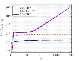
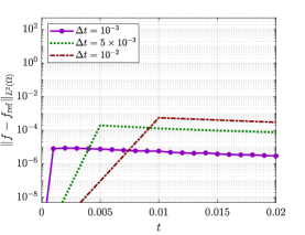
While explicit step-truncation methods have proven successful in integrating a wide variety of high-dimensional initial value problems, their effectiveness for stiff problems is limited. Indeed, the combination of non-linearity and stiffness may introduce time-step restrictions which could make explicit step-truncation integration computationally infeasible. As an example, in Figure 1 we show that the explicit step-truncation midpoint method applied to the Allen-Cahn equation

$$\frac{\partial f}{\partial t}=\varepsilon\Delta f+f-f^{3},$$ (7)

undergoes a numerical instability for $\Delta t=10^{-3}$.

         Explicit step-truncation midpoint method                       Implicit step-truncation midpoint method

Figure 1: Explicit and implicit step-truncation midpoint methods applied the Allen-Cahn equation (7) with $\varepsilon=0.1$. It is seen that the explicit step-truncation midpoint method undergoes a numerical instability for $\Delta t=10^{-3}$ while the implicit step-truncation midpoint method retains accuracy and stability for $\Delta t=10^{-3}$, and even larger time steps. Stability implicit step-truncation midpoint is studied in section 4.

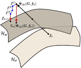
The main objective of this paper is to develop a new class of rank-adaptive implicit step-truncation algorithms to integrate high-dimensional initial value problems of the form (4) on low-rank tensor manifolds. The main idea of these new integrators is illustrated in Figure 2. Roughly speaking, implicit step-truncation method take $\bm{f}_{k}\in{\cal H}_{\bm{r}}$ (${\cal H}_{\bm{r}}$ is a HT or TT tensor manifold with multilinear rank $\bm{r}$) and $\bm{\Psi}_{\Delta t}(\bm{G},\bm{f}_{k})$ as input and generate a sequence of inexact Newton iterates ${\bm{f}}^{[j]}$ converging to a point tensor manifold ${\cal H}_{\bm{s}}$. Once ${\bm{f}}^{[j]}$ is sufficiently close to ${\cal H}_{\bm{s}}$ we project it onto the manifold via a standard truncation operation. This operation is also known as “compression step” in the HT/TT-GMRES algorithm described in [20]. Of course the computational cost of implicit step-truncation methods is higher than that of explicit step truncation methods for one single step. However, implicit methods allow to integrate stably with larger time-steps while retaining accuracy. Previous research on implicit tensor integration leveraged the Alternating Least Squares (ALS) algorithm [8, 19, 13], which essentially attempts to solve an optimization problem on a low-rank tensor manifold to compute the solution of (4) at each time step. As is well-known, ALS is equivalent to the (linear) block Gauss-Seidel iteration applied to the Hessian matrix of the residual, and can have convergence issues [45].

Figure 2: Sketch of implicit and explicit step-truncation integration methods. Given a tensor $\bm{f}_{k}$ with multilinear rank $\bm{r}$ on the tensor manifold ${\cal H}_{\bm{r}}$, we first perform an explicit time-step, e.g., with the conventional time-stepping scheme (5). The explicit step-truncation integrator then projects $\bm{\Psi}_{\Delta t}(\bm{G},\bm{f}_{k})$ onto a new tensor manifold ${\cal H}_{\bm{s}}$ (solid red line). The multilinear rank $\bm{s}$ is chosen adaptively based on desired accuracy and stability constraints [40]. On the other hand, the implicit step-truncation method takes $\bm{\Psi}_{\Delta t}(\bm{G},\bm{f}_{k})$ as input and generates a sequence of fixed-point iterates ${\bm{f}}^{[j]}$ shown as dots connected with blue lines. The last iterate is then projected onto a low rank tensor manifold, illustrated here also as a red line landing on ${\cal H}_{\bm{s}}$. This operation is equivalent to the compression step in the HT/TT-GMRES algorithm described in [20].

The paper is organized as follows. In section 1, we briefly review rank-adaptive explicit step-truncation methods, and present a new convergence proof for these methods which applies also to implicit step-truncation methods. In section 2, we discuss the proposed new algorithms for implicit step-truncation integration. In section 3 we study convergence of particular implicit step-truncation methods, namely the step-truncation implicit Euler and midpoint methods. In section 4 we prove that the stability region of an implicit step-truncation method is identical to that of the implicit method without tensor truncation. Finally, in section 5 we present numerical applications of implicit step-truncation algoritihms to stiff PDEs. In particular, we study a two-dimensional Allen-Cahn equation, a four-dimensional Fokker-Planck equation, and a six-dimensional nonlinear Schrödinger equation. We also include a brief appendix in which we discuss numerical algorithms to solve linear and nonlinear algebraic equations on tensor manifolds via the inexact Newton’s method with HT/TT-GMRES iterations.

1 Explicit step-truncation methods

In this section we briefly review explicit step-truncation methods to integrate the tensor-valued ODE (4) on tensor manifolds with variable rank. For a complete account of this theory see [40]. We begin by first discretizing the ODE in time with any standard explicit one-step method on an evenly-spaced temporal grid

$${\bm{f}}_{k+1}={\bm{\Psi}}_{\Delta t}({\bm{G}},{\bm{f}}_{k}).$$ (8)

Here, ${\bm{f}}_{k}$ denotes an approximation of the exact solution ${\bm{f}}(k\Delta t)$ for $k=1,2,...,N$, and ${\bm{\Psi}}_{\Delta t}$ is an increment function. For example, ${\bm{\Psi}}_{\Delta t}$ can be the increment function corresponding to the Euler forward method

$${\bm{\Psi}}_{\Delta t}({\bm{G}},{\bm{f}}_{k})={\bm{f}}_{k}+\Delta t{\bm{G}}({\bm{f}}_{k}).$$ (9)

In the interest of saving computational resources when iterating (8) we look for an approximation of $\bm{f}_{k}$ on a low-rank tensor manifold ${\cal H}_{\bm{r}}$ [46] with multilinear rank $\bm{r}$. ${\cal H}_{\bm{r}}$ is taken to be the manifold of Hierarchical Tucker (HT) tensors. The easiest way for approximating (8) on ${\cal H}_{\bm{r}}$ is to apply a nonlinear projection operator [24] (truncation operator)

$$\mathfrak{T}_{\bm{r}}:\mathbb{R}^{n_{1}\times n_{2}\times\cdots\times n_{d}}\to\overline{\cal H}_{\bm{r}},$$ (10)

where $\overline{\cal H}_{\bm{r}}$ denotes the closure of ${\cal H}_{\bm{r}}$. This yields the explicit step-truncation scheme

$${\bm{f}}_{k+1}={\mathfrak{T}}_{\bm{r}}\left({\bm{\Psi}}_{\Delta t}({\bm{G}},{\bm{f}}_{k})\right).$$ (11)

The rank $\bm{r}$ can vary with the time step based on appropriate error estimates as time integration proceeds [40]. We can also project $\bm{G}(\bm{f})$ onto $\overline{\cal H}_{\bm{r}}$ before applying ${\bm{\Psi}}_{\Delta t}$. With reference to (9) this yields

$$\bm{f}_{k+1}={\mathfrak{T}}_{{\bm{r}}_{2}}\left({\bm{f}}_{k}+\Delta t{\mathfrak{T}}_{{\bm{r}}_{1}}\left({\bm{G}}({\bm{f}}_{k})\right)\right).$$ (12)

Here $\bm{r}_{1}$ and ${\bm{r}}_{2}$ are truncation ranks determined by the inequalities

$$\left\|{\bm{G}}({\bm{f}}_{k})-\mathfrak{T}_{{\bm{r}}_{1}}\left({\bm{G}}({\bm{f}}_{k})\right)\right\|\leq e_{1},\qquad\left\|\widetilde{\bm{f}}_{k+1}-\mathfrak{T}_{{\bm{r}}_{2}}\left(\widetilde{\bm{f}}_{k+1}\right)\right\|\leq e_{2},$$ (13)

where $e_{1}$ and $e_{2}$ are chosen error thresholds. As before, $\bm{r}_{1}$ and $\bm{r}_{2}$ can change with every time step. In particular, if we choose $e_{1}=K_{1}\Delta t$ and $e_{2}=K_{2}\Delta t^{2}$ (with $K_{1}$ and $K_{2}$ given constants) then the step-tuncation method (12) is convergent (see [40] for details). More generally, let

$$\bm{f}_{k+1}={\bm{\Phi}}_{\Delta t}({\bm{G}},{\bm{f}_{k}},{\bm{e}})$$ (14)

be an explicit step-truncation method in which all we project all $\bm{G}(\bm{f}_{k})$ appearing in the increment function ${\bm{\Psi}}_{\Delta t}({\bm{G}},{\bm{f}}_{k})$ onto tensor manifolds $\overline{{\cal H}}_{\bm{r}_{i}}$ by setting suitable error thresholds $\bm{e}=(e_{1},e_{2},\ldots)$. For instance, if ${\bm{\Psi}}_{\Delta t}$ is defined by the explicit midpoint method, i.e.,

$${\bm{\Psi}}_{\Delta t}\left({\bm{G}},{\bm{f}_{k}}\right)=\bm{f}_{k}+\bm{G}\left(\bm{f}_{k}+\frac{\Delta t}{2}\bm{G}(\bm{f}_{k})\right)$$ (15)

then

$${\bm{\Phi}}_{\Delta t}({\bm{G}},{\bm{f}_{k}},{\bm{e}})=\mathfrak{T}_{\bm{r}_{3}}\left(\bm{f}_{k}+\mathfrak{T}_{\bm{r}_{2}}\left[\bm{G}\left(\bm{f}_{k}+\frac{\Delta t}{2}\mathfrak{T}_{\bm{r}_{1}}\left[\bm{G}(\bm{f}_{k})\right]\right)\right]\right),$$ (16)

where $\bm{e}=(e_{1},e_{2},e_{3})$ is a vector collecting the truncation error thresholds yielding the multilinear ranks $\bm{r}_{1}$, $\bm{r}_{2}$ and $\bm{r}_{3}$. By construction, step-truncation methods of the form (14) satisfy

$$\left\|{\bm{\Psi}}_{\Delta t}({\bm{G}},{\bm{f}})-{\bm{\Phi}}_{\Delta t}({\bm{G}},{\bm{f}},{\bm{e}})\right\|\leq R({\bm{e}}),$$ (17)

where $R({\bm{e}})$ is the error due to tensor truncation. We close this section with a reformulation of the convergence theorem for explicit step-truncation methods in [40], which applies also to implicit methods.

Theorem 1 (Convergence of step-truncation methods).

Let ${\bm{\varphi}}_{\Delta t}({\bm{G}},{\bm{f}})$ be the one-step exact flow map defined by (4), and ${\bm{\Phi}}_{\Delta t}({\bm{G}},{\bm{f}},{\bm{e}})$ be the increment function of a step-truncation method with local error of order $p$, i.e.,

$$\left\|{\bm{\varphi}}_{\Delta t}({\bm{G}},{\bm{f}})-{\bm{\Phi}}_{\Delta t}({\bm{G}},{\bm{f}},{\bm{e}})\right\|\leq K\Delta t^{p+1}\quad\text{as}\quad\Delta t\rightarrow 0.$$ (18)

If there exist truncation errors ${\bm{e}}={\bm{e}}(\Delta t)$ (function of $\Delta t$) and constants $C,E>0$ (dependent on ${\bm{G}}$) so that the stability condition

$$\left\|{\bm{\Phi}}_{\Delta t}({\bm{G}},\hat{\bm{f}},{\bm{e}})-{\bm{\Phi}}_{\Delta t}({\bm{G}},\tilde{\bm{f}},{\bm{e}})\right\|\leq(1+C\Delta t)\left\|\hat{\bm{f}}-\tilde{\bm{f}}\right\|+E\Delta t^{m+1}$$ (19)

holds as $\Delta t\rightarrow 0$, then the step-truncation method is convergent with order $z=\text{min}(m,p)$.

Proof. Under the assumption that $\Delta t$ is small enough for our stability and consistency to hold, we proceed by induction on the number of steps. The one-step case coincides with the consistency condition. Next, we assume that

$$\left\|{\bm{\varphi}}_{\Delta t(N-1)}({\bm{G}},{\bm{f}}_{0})-{\bm{f}}_{N-1}\right\|\leq Q_{N-1}\Delta t^{z}.$$ (20)

Let $T=N\Delta t$ be the final integration time. By applying triangle inequality and the semigroup property of the flow map,

$$\left\|{\bm{\varphi}}_{T}({\bm{G}},{\bm{f}}_{0})-{\bm{\Phi}}_{\Delta t}({\bm{G}},{\bm{f}}_{N-1},{\bm{e}})\right\| \leq\left\|{\bm{\varphi}}_{\Delta t}({\bm{G}},{\bm{\varphi}}_{\Delta t(N-1)}({\bm{G}},{\bm{f}}_{0}))-{\bm{\Phi}}_{\Delta t}({\bm{G}},{\bm{\varphi}}_{\Delta t(N-1)}({\bm{G}},{\bm{f}}_{0}),{\bm{e}})\right\|$$

$$\qquad+\left\|{\bm{\Phi}}_{\Delta t}({\bm{G}},{\bm{\varphi}}_{\Delta t(N-1)}({\bm{G}},{\bm{f}}_{0}),{\bm{e}})-{\bm{\Phi}}_{\Delta t}({\bm{G}},{\bm{f}}_{N-1},{\bm{e}})\right\|.$$ (21)

Using the consistency condition (18) we can bound the first term at the right hand side of (21) by $K_{N-1}\Delta t^{p+1}$, where $K_{N-1}$ represents a local error coefficient. On the other hand, using the stability condition (19) we can can bound the second term at the right hand side of (21) as

$$\left\|{\bm{\Phi}}_{\Delta t}({\bm{G}},{\bm{\varphi}}_{\Delta t(N-1)}({\bm{G}},{\bm{f}}_{0}),{\bm{e}})-{\bm{\Phi}}_{\Delta t}({\bm{G}},{\bm{f}}_{N-1},{\bm{e}})\right\|\leq(1+C\Delta t) \left\|{\bm{\varphi}}_{\Delta t(N-1)}({\bm{G}},{\bm{f}}_{0})-{\bm{f}}_{N-1}\right\|$$

$$+E\Delta t^{m+1}.$$ (22)

A substitution of (22) and (20) into (21) yields

$$\left\|{\bm{\varphi}}_{T}({\bm{G}},{\bm{f}}_{0})-{\bm{\Phi}}_{\Delta t}({\bm{G}},{\bm{f}}_{N-1},{\bm{e}})\right\| \leq K_{N-1}\Delta t^{p+1}+(1+C\Delta t)Q_{N-1}\Delta t^{z}+E\Delta t^{m+1}.$$

Recalling that $z=\text{min}(m,p)$ completes the proof.

∎

We remark that the above proof may be modified to include explicit step-truncation linear multi-step methods, i.e., step-truncation Adams methods. To this end, it is sufficient to replace ${\bm{f}}_{k}$ with the vector $({\bm{f}}_{k-s},{\bm{f}}_{k-s+1},\dots,{\bm{f}}_{k})$ and the stability condition (19) with

$$\left\|{\bm{\Phi}}_{\Delta t}({\bm{G}},{\bm{\hat{f}}}_{1},{\bm{\hat{f}}}_{2},\dots,{\bm{\hat{f}}}_{s},{\bm{e}})-{\bm{\Phi}}_{\Delta t}({\bm{G}},{\bm{\tilde{f}}}_{1},{\bm{\tilde{f}}}_{2},\dots,{\bm{\tilde{f}}}_{s},{\bm{e}})\right\|\leq\left\|{\bm{\hat{f}}}_{s}-{\bm{\tilde{f}}}_{s}\right\|+\sum_{j=1}^{s}C_{j}\Delta t\left\|{\bm{\hat{f}}}_{j}-{\bm{\tilde{f}}}_{j}\right\|+E\Delta t^{m+1}.$$ (23)

We then have an analogous theorem proven using an inductive argument based on the initial conditions ${\bm{f}}(0),{\bm{f}}(\Delta t),\dots,{\bm{f}}((s-1)\Delta t)$.

2 Implicit step-truncation methods

To introduce implicit step-truncation tensor methods, let us begin with the standard Euler backward scheme

$${\bm{f}}_{k+1}={\bm{f}}_{k}+\Delta t{\bm{G}}({\bm{f}}_{k+1}),$$ (24)

and the associated root-finding problem

$$\bm{H}_{k}(\bm{f}_{k+1})={\bm{f}}_{k+1}-{\bm{f}}_{k}-\Delta t{\bm{G}}({\bm{f}}_{k+1})={\bm{0}}.$$ (25)

Equation (25) allows us to compute $\bm{f}_{k+1}$ as a zero of the function $\bm{H}_{k}$. This can be done, e.g., using the Netwon’s method with initial guess $\bm{f}^{[0]}_{k+1}=\bm{f}_{k}$. As is well-known, if the Jacobian of $\bm{H}_{k}$ is invertible within a neighborhood of $\bm{f}_{k}$, then the implicit function theorem guarantees the existence of a locally differentiable (in some neighborhood of $\bm{f}_{k}$) nonlinear map ${\bm{\Theta}}_{\Delta t}$ depending on $\bm{G}$ such that

$${\bm{f}}_{k+1}={\bm{\Theta}}_{\Delta t}\left({\bm{G}},{\bm{f}}_{k}\right).$$ (26)

In the setting of Newton’s method described above, the map ${\bm{\Theta}}_{\Delta t}$ is computed iteratively. An implicit step-truncation scheme can be then formulated by applying the tensor truncation operator $\mathfrak{T}_{\bm{r}}$ to the right hand side of (26), i.e.,

$${\bm{f}}_{k+1}={\mathfrak{T}}_{{\bm{r}}}\left({\bm{\Theta}}_{\Delta t}\left({\bm{G}},{\bm{f}}_{k}\right)\right).$$ (27)

The tensor truncation rank $\bm{r}$ can be selected based on the inequality

$$\|{\mathfrak{T}}_{{\bm{r}}}({\bm{\Theta}}_{\Delta t}({\bm{G}},{\bm{f}}_{k}))-{\bm{\Theta}}_{\Delta t}({\bm{G}},{\bm{f}}_{k})\|\leq A\Delta t^{2}.$$ (28)

It was shown in [40] that this yields an order one (in time) integration scheme. Of course, if the Jacobian of $\bm{H}_{k}$ in equation (25) can be computed and stored in computer memory, then we can approximate $\bm{f}_{k+1}={\bm{\Theta}}_{\Delta t}({\bm{G}},{\bm{f}}_{k})$ for any given $\bm{f}_{k}$ and $\bm{G}$ using Newton’s iterations. However, the exact Newton’s method is not available to us in the high-dimensional tensor setting.

Hence, we look for an approximation of ${\bm{\Theta}}_{\Delta t}({\bm{G}},{\bm{f}}_{k})$ computed using the inexact Newton method [17]. For the inexact matrix inverse step, we apply the relaxed TT-GMRES algorithm described in [20]. This is an iterative method for the solution of linear equations which makes use of an inexact matrix-vector product defined by low-rank truncation. Though the algorithm was developed for TT tensors, it may be also applied to HT tensors without significant changes.

In Appendix A we describe the inexact Newton’s method with HT/TT-GMRES iterations to solve an arbitrary algebraic equation of the form $\bm{H}_{k}(\bm{f})=\bm{0}$ (e.g., equation (25)) on a tensor manifold with a given rank. The algorithm can be used to approximate the mapping ${\bm{\Theta}}_{\Delta t}({\bm{G}},{\bm{f}}_{k})$ corresponding to any implicit integrator, and it returns a tensor with can be then truncated further as in (27). This operation is equivalent to the so-called “compression step” in [20] and it is described in detail in the next section.

2.1 The compression step

While increasing the tensor rank may be necessary for convergence of the HT/TT-GMRES iterations, it is possible that we raise the rank by more than is required for the desired order of accuracy in a single time step. Therefore, it is convenient to apply an additional tensor truncation after computing, say, $j$ steps of the HT inexact Newton’s method which returns ${\bm{f}}_{k+1}^{[j]}$. This is the same as the “compression step” at the end of HT/TT-GMRES algorithm as presented in [20]. This gives us our final estimate of ${\bm{f}}((k+1)\Delta t)$ as

$${\bm{f}}_{k+1}={\mathfrak{T}}_{\bm{r}}\left({\bm{f}}_{k+1}^{[j]}\right),\qquad\left\|{\mathfrak{T}}_{\bm{r}}\left({\bm{f}}_{k+1}^{[j]}\right)-{\bm{f}}_{k+1}^{[j]}\right\|\leq e_{\bm{r}}.$$ (29)

Regarding the selection of the truncation error $e_{\bm{r}}$ we proceed as follows. Suppose that ${\bm{\Psi}}_{\Delta t}({\bm{G}},{\bm{f}}_{k})$ is an explicit integration scheme of the same order (or higher) than the implicit scheme being considered. Then we can estimate local error as

$$\left\|{\bm{f}}_{k+1}^{[j]}-{\bm{f}}((k+1)\Delta t)\right\| \leq\left\|{\bm{f}}_{k+1}^{[j]}-{\bm{\Psi}}_{\Delta t}({\bm{G}},{\bm{f}}_{k})\right\|+\left\|{\bm{\Psi}}_{\Delta t}({\bm{G}},{\bm{f}}_{k})-{\bm{f}}((k+1)\Delta t)\right\|$$

$$=\left\|{\bm{f}}_{1}^{[j]}-{\bm{\Psi}}_{\Delta t}({\bm{G}},{\bm{f}}_{k})\right\|+O(\Delta t^{p+1}),$$ (30)

Thus, we may roughly estimate the local truncation error and set this as the chosen error for approximation to HT or TT rank $\bm{r}$ using

$${e}_{\bm{r}}=\left\|{\bm{f}}_{k+1}^{[j]}-{\bm{\Psi}}_{\Delta t}({\bm{G}},{\bm{f}}_{k})\right\|.$$ (31)

We may drop more singular values than needed, especially if the choice of $\Delta t$ is outside the region of stability of the explicit scheme ${\bm{\Psi}}_{\Delta t}({\bm{G}},{\bm{f}}_{k})$. However, this estimate guarantees that we do not change the overall convergence rate. Moreover, it cannot impact stability of the implicit step-truncation integrator since the compression step has operator norm equal to one, regardless of the rank chosen. This statement is supported by the analysis presented in [41] for step-truncation linear multi-step methods. In all our numerical experiments we use the explicit step-truncation midpoint method to estimate local error, i.e., ${\bm{\Psi}}_{\Delta t}({\bm{G}},{\bm{f}}_{k})$ in (31) is set as in (15).

3 Convergence analysis of implicit step-truncation methods

In this section we show that applying the inexact Newton iterations with HT/TT-GMRES to the implicit Euler and the implicit midpoint methods result in implicit step-truncation schemes that fit into the framework of Theorem 1, and therefore are convergent.

3.1 Implicit step-truncation Euler method

Consider the implicit Euler scheme (25), and suppose that the solution of the nonlinear equation $\bm{H}_{k}(\bm{f}_{k+1})=\bm{0}$ is computed using the inexact Newton method with HT/TT-GMRES iterations as discussed in Appendix A. Let ${\bm{f}}_{k+1}^{[j]}$ ($j=1,2,\ldots,$) be the sequence of tensors generated by the algorithm and approximating $\bm{f}_{k+1}$ (exact solution of $\bm{H}_{k}(\bm{f}_{k+1})=\bm{0}$). We set a stopping criterion for terminating Newton’s iterations based on the residual, i.e.,

$$\left\|{\bm{H}}_{k}\left({\bm{f}}_{k+1}^{[j]}\right)\right\|\leq\varepsilon_{\text{tol}}.$$ (32)

This allows us to adjust the rank of ${\bm{f}}_{k+1}^{[j]}$ from one time step to the next, depending on the desired accuracy $\varepsilon_{\text{tol}}$. Our goal is to analyze convergence of such rank-adaptive implicit method when a finite number of contraction mapping steps is taken. To this end, we will fit the method into the framework of Theorem 1. We begin by noticing that

$$\left\|{\bm{f}}_{k+1}-{\bm{f}}_{k+1}^{[j]}\right\| =\left\|{\bm{H}}_{k}^{-1}\left({\bm{H}}_{k}\left({\bm{f}}_{k+1}\right)\right)-{\bm{H}}_{k}^{-1}\left({\bm{H}}_{k}\left({\bm{f}}_{k+1}^{[j]}\right)\right)\right\|\leq L_{{\bm{H}}_{k}^{-1}}\left\|{\bm{H}}\left({\bm{f}}_{k+1}^{[j]}\right)\right\|\leq L_{{\bm{H}}_{k}^{-1}}\varepsilon_{\text{tol}},$$ (33)

where $L_{{\bm{H}}_{k}^{-1}}$ is the local Lipschitz constant of the smooth inverse map $H^{-1}_{k}$, the existence of which is granted by the inverse function theorem. This allows us to write the local truncation error as

$$\left\|{\bm{f}}(\Delta t)-{\bm{f}}_{1}^{[j]}\right\| \leq\left\|{\bm{f}}(\Delta t)-{\bm{f}}_{1}\right\|+\left\|{\bm{f}}_{1}-{\bm{f}}_{1}^{[j]}\right\|\leq K_{1}\Delta t^{2}+L_{{\bm{H}}^{-1}}\varepsilon_{\text{tol}},$$ (34)

where $K_{1}$ is a local error coefficient. In order to maintain order one convergence, we require that $\varepsilon_{\text{tol}}\leq K\Delta t^{2}$ for some constant $K\geq 0$.

Next, we discuss the stability condition (19) in the context of the implicit step-truncation Euler scheme, assuming that ${\bm{f}}_{k+1}$ can be found exactly by the inexact Newton’s method, eventually after an infinite number of iterations. Denote by ${\bm{\hat{f}}}_{0}$, ${\bm{\tilde{f}}}_{0}$ two different initial conditions. Performing one step of the standard implicit Euler’s method yields the following bound

$$\left\|{\bm{\hat{f}}}_{1}-{\bm{\tilde{f}}}_{1}\right\|=\left\|\left({\bm{\hat{f}}}_{0}+\Delta t{\bm{G}}({\bm{\hat{f}}}_{1})\right)-\left({\bm{\tilde{f}}}_{0}+\Delta t{\bm{G}}({\bm{\tilde{f}}}_{1})\right)\right\|\leq\left\|{\bm{\hat{f}}}_{0}-{\bm{\tilde{f}}}_{0}\right\|+\Delta tL_{\bm{G}}\left\|{\bm{\hat{f}}}_{1}-{\bm{\tilde{f}}}_{1}\right\|.$$

where $L_{\bm{G}}$ is the Lipschitz constant of $\bm{G}$. By collecting like terms, we obtain

$$\left\|{\bm{\hat{f}}}_{1}-{\bm{\tilde{f}}}_{1}\right\|\leq\frac{1}{1-\Delta tL_{\bm{G}}}\left\|{\bm{\hat{f}}}_{0}-{\bm{\tilde{f}}}_{0}\right\|\leq(1+2\Delta tL_{\bm{G}})\left\|{\bm{\hat{f}}}_{0}-{\bm{\tilde{f}}}_{0}\right\|.$$ (35)

The last inequality comes by noting that $1/({1-\Delta tL_{\bm{G}}})\leq 1+2\Delta tL_{\bm{G}}$ when $\Delta t$ is sufficiently small, i.e., $\Delta t\leq 1/(2L_{\bm{G}})$. This is zero-stability condition, i.e., a stability condition that holds for small $\Delta t$, which will be used for convergence analysis. Regarding the behavior of the scheme for finite $\Delta t$ we will show in section 4 that the implicit step-truncation Euler scheme is unconditionally stable. Next, we derive a stability condition of the form (35) when the root of $\bm{H}_{k}(\bm{f}_{k+1})=\bm{0}$ is computed with the inexact Newton’s method with HT/TT-GMRES iterations. In this case we have

$$\left\|{\bm{\hat{f}}}_{1}^{[j]}-{\bm{\tilde{f}}}_{1}^{[m]}\right\| \leq\left\|{\bm{\hat{f}}}_{1}^{[j]}-{\bm{\hat{f}}}_{1}^{[\infty]}\right\|+\left\|{\bm{\hat{f}}}_{1}^{[\infty]}-{\bm{\tilde{f}}}_{1}^{[\infty]}\right\|+\left\|{\bm{\tilde{f}}}_{1}^{[m]}-{\bm{\tilde{f}}}_{1}^{[\infty]}\right\|$$

$$=\left\|{\bm{\hat{f}}}_{1}^{[j]}-{\bm{\hat{f}}_{1}}\right\|+\left\|{\bm{\hat{f}}_{1}}-{\bm{\tilde{f}}_{1}}\right\|+\left\|{\bm{\tilde{f}}}_{1}^{[m]}-{\bm{\tilde{f}}_{1}}\right\|$$

$$\leq(1+2L_{\bm{G}}\Delta t)\left\|{\bm{\hat{f}}}_{0}-{\bm{\tilde{f}}}_{0}\right\|+2L_{{\bm{H}}^{-1}}\varepsilon_{\text{tol}}.$$ (36)

Thus, the stability condition is satisfied by the same condition on $\varepsilon_{\text{tol}}$ that satisfies the first-order consistency condition (34), i.e., $\varepsilon_{\text{tol}}\leq K\Delta t^{2}$. At this point we apply Theorem 1 with consistency and stability conditions (18)-(19) replaced by (34) and (36), respectively, and conclude that the implicit step-truncation Euler scheme is convergent with order one if $\varepsilon_{\text{tol}}\leq K\Delta t^{2}$.

Remark 1.

When $\bm{G}$ is linear, i.e., when the tensor ODE (4) is linear, then we may apply HT/TT-GMRES algorithm in Appendix A without invoking Newton’s method. In this case, the local error coefficient $L_{{\bm{H}}_{k}^{-1}}$ can be exchanged for the coefficient of $\varepsilon$ at the right side of inequality (78).

3.2 Implicit step-truncation midpoint method

The implicit midpoint rule [26],

$${\bm{f}}_{k+1}={\bm{f}}_{k}+\Delta t{\bm{G}}\left(\frac{1}{2}({\bm{f}}_{k}+{\bm{f}}_{k+1})\right),$$ (37)

is a symmetric and symplectic method of order 2. By introducing

$${\bm{H}}_{k}\left({\bm{f}}_{k+1}\right)={\bm{f}}_{k+1}-{\bm{f}}_{k}-\Delta t{\bm{G}}\left(\frac{1}{2}({\bm{f}}_{k}+{\bm{f}}_{k+1})\right)={\bm{0}}$$ (38)

we again see the implicit method as a root finding problem at each time step. To prove convergence of the implicit step-truncation midpoint method we follow the same steps described in the previous section. To this end, consider the sequence of tensors ${\bm{f}}^{[j]}_{k+1}$ generated by the inexact Newton method with HT/TT-GMRES iterations (see Appendix A) applied to (38). The sequence of tensors ${\bm{f}}^{[j]}_{k+1}$ approximates $\bm{f}_{k+1}$ satisfying (38). As before, we terminate the inexact Newton’s iterations as soon as condition (32) is satisfied. By repeating the same steps that led us to inequality (33), we have

$$\left\|{\bm{f}}(\Delta t)-{\bm{f}}_{1}^{[j]}\right\|\leq K_{1}\Delta t^{3}+L_{{\bm{H}}_{k}^{-1}}\varepsilon_{\text{tol}}.$$ (39)

Hence, setting the stopping tolerance as $\varepsilon_{\text{tol}}\leq K\Delta t^{3}$ we get second-order consistency. We use this to determine the stability condition (19). As before, we derive the condition for when the zero of (38) is exact. Denote by ${\bm{\hat{f}}}_{0}$, ${\bm{\tilde{f}}}_{0}$ two different initial conditions. Performing one step of the standard implicit midpoint method yields the following bound

$$\left\|{\bm{\hat{f}}}_{1}-{\bm{\tilde{f}}}_{1}\right\|\leq\left(1+\Delta t\frac{L_{\bm{G}}}{2}\right)\left\|{\bm{\hat{f}}}_{0}-{\bm{\tilde{f}}}_{0}\right\|+\Delta t\frac{L_{\bm{G}}}{2}\left\|{\bm{\hat{f}}}_{1}-{\bm{\tilde{f}}}_{1}\right\|.$$

By collecting like terms we see that when $\Delta t\leq 1/L_{\bm{G}}$,

$$\left\|{\bm{\hat{f}}}_{1}-{\bm{\tilde{f}}}_{1}\right\| \leq\frac{2+\Delta tL_{\bm{G}}}{2-\Delta tL_{\bm{G}}}\left\|{\bm{\hat{f}}}_{0}-{\bm{\tilde{f}}}_{0}\right\|$$

$$\leq\left(1+\Delta t\frac{3L_{\bm{G}}}{2}\right)\left\|{\bm{\hat{f}}}_{0}-{\bm{\tilde{f}}}_{0}\right\|.$$ (40)

The zero-stability condition for the implicit step-truncation midpoint method can now be found by repeating the arguments of inequality (36). This gives

$$\left\|{\bm{\hat{f}}}_{1}^{[j]}-{\bm{\tilde{f}}}_{1}^{[m]}\right\|\leq(1+L_{\bm{G}}\Delta t)\left\|{\bm{\hat{f}}}_{0}-{\bm{\tilde{f}}}_{0}\right\|+2L_{{\bm{H}}_{k}^{-1}}\varepsilon_{\text{tol}}.$$ (41)

Thus, the stability condition is satisfied by the same condition on $\varepsilon_{\text{tol}}$ that satisfies the second-order consistency condition (39), i.e., $\varepsilon_{\text{tol}}\leq K\Delta t^{3}$. At this point we apply Theorem 1 with consistency and stability conditions (18)-(19) replaced by (39) and (41), respectively, and conclude that the implicit step-truncation midpoint scheme is convergent with order two if $\varepsilon_{\text{tol}}\leq K\Delta t^{3}$.

4 Stability analysis

We now address absolute stability of the proposed implicit step-truncation methods. This notion of stability is related to the behavior of the schemes when applied the initial value problem

$$\frac{d{\bm{f}}}{dt}={\bm{L}}{\bm{f}},\quad{\bm{f}}(0)={\bm{f}}_{0}$$ (42)

where $\bm{L}$ is a linear operator with eigenvalues in in the left half complex plane. After applying any standard implicit time stepping scheme, we end up with a system of linear equations of the form

$${\bm{A}}{\bm{f}}_{k+1}={\bm{W}}{\bm{f}}_{k}.$$ (43)

Specifically, for the implicit Euler we have ${\bm{A}}={\bm{I}}-\Delta t{\bm{L}}$, ${\bm{W}}={\bm{I}}$ while for the implicit midpoint method we have ${\bm{A}}={\bm{I}}-0.5\Delta t{\bm{L}}$, ${\bm{W}}={\bm{I}}+0.5\Delta t{\bm{L}}$. As is well known, both implicit Euler and Implicit midpoint are unconditionally stable, in the sense that for any $\Delta t>0,$ $\|{\bm{f}}_{k}\|\rightarrow 0$ as $k\rightarrow\infty$. One way of proving this is by noting that whenever the eigenvalues of ${\bm{L}}$ have negative real part, we get

$$\|{\bm{A}}^{-1}{\bm{W}}\|<1,$$ (44)

and therefore the mapping ${\bm{A}}^{-1}{\bm{W}}$ is contractive. This implies the sequence $\bm{f}_{k}$ defined by (43) converges to zero. The following theorem characterizes what happens when we exchange exact matrix inverse ${\bm{A}}^{-1}$ with an inexact inverse computed by tensor HT/TT-GMRES iterations.

Theorem 2 (Absolute stability of implicit step-truncation methods).

Consider an implicit time stepping scheme of the form (43), and suppose that $\|{\bm{A}}^{-1}{\bm{W}}\|<1$. Denote by ${\hat{\bm{f}}}_{k}$ the solution of $\bm{A}{\hat{\bm{f}}}_{k}={\bm{W}}{\hat{\bm{f}}}_{k-1}$ ($k=1,2,\ldots$) obtained with the HT/TT-GMRES tensor solver described in Appendix A, with $m$ Krylov iterations and stopping tolerance $\eta$. If

$$\left\|{\bm{A}}{\hat{\bm{f}}}_{k}-{\bm{W}}{\hat{\bm{f}}}_{k-1}\right\|\leq m\|{\bm{A}}\|\|{\bm{A}}^{-1}\|\eta,$$ (45)

then the distance between ${\hat{\bm{f}}}_{k}$ and the exact solution ${\bm{f}}_{k}=\bm{A}^{-1}\bm{W}\bm{f}_{k-1}$ can be bounded as

$$\left\|{\hat{\bm{f}}}_{k}-{\bm{f}}_{k}\right\|\leq\frac{m\|{\bm{A}}\|\|{\bm{A}}^{-1}\|^{2}}{1-\|{\bm{A}}^{-1}{\bm{W}}\|}\eta.$$ (46)

Note that (46) implies that $\left\|{\hat{\bm{f}}}_{k}\right\|=O(\eta)$ as $k\rightarrow\infty$. In the context of HT/TT-GMRES iterations, the number $\eta$ can be controlled by setting the stopping tolerance in Lemma 1 (Appendix A) as

$$\varepsilon_{k}=\frac{\eta}{\left\|{\bm{W}}{\hat{\bm{f}}}_{k}\right\|}$$ (47)

at each time step $k$.

Proof. The proof follows from a straightforward inductive argument. For $k=1$ we have

$${\hat{\bm{f}}}_{1}-{\bm{f}}_{1} =\bm{A}^{-1}\bm{A}{\hat{\bm{f}}}_{1}-\bm{A}^{-1}\bm{W}{\bm{f}}_{0}$$

$$=\bm{A}^{-1}\left(\bm{A}{\hat{\bm{f}}}_{1}-\bm{W}{\bm{f}}_{0}\right).$$ (48)

By using (45), we can bound $\left\|{\hat{\bm{f}}}_{1}-{\bm{f}}_{1}\right\|$ as

$$\left\|{\hat{\bm{f}}}_{1}-{\bm{f}}_{1}\right\|\leq m\|{\bm{A}}\|\|{\bm{A}}^{-1}\|^{2}\eta.$$ (49)

For $k=2$ we have

$$\left\|{\bm{\hat{f}}}_{2}-{\bm{f}}_{2}\right\| \leq\left\|{\bm{\hat{f}}}_{2}-{\bm{A}}^{-1}{\bm{W}}{\bm{\hat{f}}}_{1}\right\|+\left\|{\bm{A}}^{-1}{\bm{W}}{\bm{\hat{f}}}_{1}-{\bm{f}}_{2}\right\|$$

$$=\left\|{\bm{\hat{f}}}_{2}-{\bm{A}}^{-1}{\bm{W}}{\bm{\hat{f}}}_{1}\right\|+\left\|{\bm{A}}^{-1}{\bm{W}}{\bm{\hat{f}}}_{1}-{\bm{A}}^{-1}{\bm{W}}{\bm{f}}_{1}\right\|$$

$$\leq m\|{\bm{A}}\|\|{\bm{A}}^{-1}\|^{2}\eta+\|{\bm{A}}^{-1}{\bm{W}}\|\left\|{\hat{\bm{f}}}_{1}-{\bm{f}}_{1}\right\|$$

$$\leq\left(1+\|{\bm{A}}^{-1}{\bm{W}}\|\right)m\|{\bm{A}}\|\|{\bm{A}}^{-1}\|^{2}\eta,$$

where the last inequality follows from (49). More generally,

$$\left\|{\bm{\hat{f}}}_{k-1}-{\bm{f}}_{k-1}\right\|\leq m\|{\bm{A}}\|\|{\bm{A}}^{-1}\|^{2}\eta\sum_{j=0}^{k-2}\|{\bm{A}}^{-1}{\bm{W}}\|^{j}.$$ (50)

Repeating the string of inequalities above and replacing the right sum with the inductive hypothesis, we obtain

$$\left\|{\bm{\hat{f}}}_{k}-{\bm{f}}_{k}\right\| \leq m\|{\bm{A}}\|\|{\bm{A}}^{-1}\|^{2}\eta\sum_{j=0}^{k-1}\|{\bm{A}}^{-1}{\bm{W}}\|^{j}$$

$$\leq\frac{m\|{\bm{A}}\|\|{\bm{A}}^{-1}\|^{2}}{1-\|{\bm{A}}^{-1}{\bm{W}}\|}\eta,$$ (51)

which completes the proof.

∎

Recall that the stability region of an explicit step-truncation method is the same as the corresponding method without truncation [41, 40]. Similarly, Theorem 2 shows that the stability region of an implicit step-truncation method is identical to the corresponding method without truncation, though by relaxing accuracy we see that instead our iterates decay to within the solver tolerance of zero rather than converging to zero in an infinite time horizon. In other words, both implicit step-truncation Euler and implicit step-truncation midpoint methods are unconditionally stable. However, if the tolerance of HT/TT-GMRES is set too large, then we could see poor stability behavior akin to an explicit method.

5 Numerical results

In this section we study the performance of the proposed implicit step-truncation methods in three numerical applications involving time-dependent PDEs. Specifically, we study the Allen-Cahn equation [35] in two spatial dimensions, the Fokker-Planck equation [39] in four dimensions, and the nonlinear Schrödinger equation [44] in six dimensions.

5.1 Allen-Cahn equation

The Allen-Cahn equation is a reaction-diffusion equation that describes the process of phase separation in multi-component alloy systems [1, 2]. In its simplest form, the equation has a cubic polynomial non-linearity (reaction term) and a diffusion term [29], i.e.,

$$\frac{\partial f}{\partial t}=\varepsilon\Delta f+f-f^{3}.$$ (52)

          ST Implicit Euler                                                    ST Implicit Midpoint

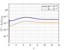
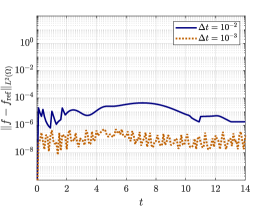
Figure 3: Error versus time for step-truncation numerical solutions of Allen-Cahn equation (57) in dimension $d=2$ with initial condition (53).

          ST Implicit Euler                                                    ST Implicit Midpoint

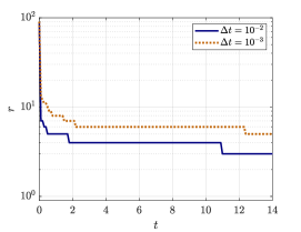
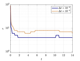
Figure 4: Rank versus time for step-truncation numerical solutions of Allen-Cahn equation (57) in dimension $d=2$ with initial condition (53).

In our application, we set $\varepsilon=0.1$, and solve (52) on the two-dimensional flat torus $\Omega=[0,2\pi]^{2}$. We employ a second order splitting [22] method to solve the Laplacian $\Delta f$ as a fixed rank temporal integration and and cubic $f-f^{3}$ term using our rank adaptive integration. The initial condition is set as

$$f_{0}(x,y)=u(x,y)-u(x,2y)+u(3x+\pi,3y+\pi)-2u(4x,4y)+2u(5x,5y),$$ (53)

where

$$u(x,y)=\frac{\left[e^{-\tan^{2}(x)}+e^{-\tan^{2}(y)}\right]\sin(x)\sin(y)}{1+e^{|\csc(-x/2)|}+e^{|\csc(-y/2)|}}.$$ (54)

We discretize (52) in space using the two-dimensional Fourier pseudospectral collocation method [27] with $257\times 257$ points in $\Omega=[0,2\pi]^{2}$. This results in a matrix ODE in the form of (4). We truncate the initial condition to absolute and relative SVD tolerances of $10^{-9}$, which yields an initial condition represented by a $257\times 257$ matrix of rank $90$. We also computed a benchmark solution of the matrix ODE using a variable step RK4 method with absolute tolerance set to $10^{-14}$. We denote the benchmark solution as $f_{\rm ref}$. In Figure 3 we observe the transient accuracy of our order one and order two implicit methods. The stopping tolerance for inexact Newton’s iterations is set to $\varepsilon_{\rm tol}=2.2\times 10^{-8}$, while and HT/TT-GMRES relative error is chosen as $\eta=10^{-3}$. Time integration was halted at $t=14$. After this time, the system is close to steady state and the errors stay bounded near the final values plotted Figure 3. Similarly, the rank also levels out around $t=14$. In Figure 4, we plot temporal evolution of the rank for both the implicit step-truncation Euler and midpoint methods.

Due to the smoothing properties of the Laplacian, the high frequencies in the initial condition quickly decay and, correspondingly, the rank drops significantly within the first few time steps. Due to the rapidly decaying rank for this problem, we have plotted it in log scale. In Figure 5, we provide a comparison between the rank-adaptive implicit step-truncation midpoint method we propose here and the rank-adaptive explicit step-truncation midpoint method

$${\bm{f}}_{k+1}={\mathfrak{T}}_{{\bm{r}_{3}}}\left({\bm{f}}_{k}+\Delta t{\mathfrak{T}}_{{\bm{r}_{2}}}\left({\bm{G}}\left({\bm{f}}_{k}+\frac{\Delta t}{2}{\mathfrak{T}}_{{\bm{r}_{1}}}({\bf G}({\bm{f}}_{k}))\right)\right)\right),$$ (55)

which was recently studied in [40]. The truncation ranks $\bm{r}_{1}$, $\bm{r}_{2}$, and $\bm{r}_{3}$ time-dependent and satisfy the order conditions

$$\varepsilon_{{\bm{r}_{3}}}\leq A\Delta t^{3},\qquad\varepsilon_{{\bm{r}_{2}}}\leq B\Delta t^{2},\qquad\varepsilon_{{\bm{r}_{1}}}\leq G\Delta t.$$ (56)

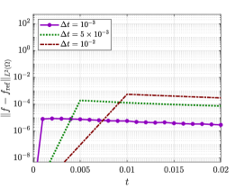
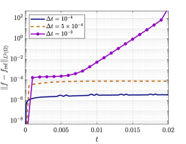
Such conditions guarantee that the scheme (55) is second-order convergent (see [40]). Figure 5 shows that the explicit step-truncation midpoint method undergoes a numerical instability for $\Delta t=10^{-3}$. Indeed it is a conditionally stable method. The explicit step-truncation midpoint method also has other issues. In particular, in the rank-adaptive setting we consider here, we have that in the limit $\Delta t\rightarrow 0$ the parameters $\varepsilon_{{\bm{r}_{1}}}$, $\varepsilon_{{\bm{r}_{2}}}$ and $\varepsilon_{{\bm{r}_{3}}}$ all go to zero (see equation (56)). This implies that the truncation operators may retain all singular values, henceforth maxing out the rank and thereby giving up all computational gains of low-rank tensor compression. On the other hand, if $\Delta t$ is too large, then one we have stability issues as discussed above. Indeed, we see both these problems with the explicit step-truncation midpoint method, giving only a relatively narrow region of acceptable time step sizes in which the method is effective.

In Table 1 we provide a comparison between explicit and implicit step-truncation midpoint methods in terms of computational cost (CPU-time on an Intel Core I9-7980XE workstation) and accuracy at time $t=14$. It is seen that the implicit step-truncation midpoint method is roughly 20 to 30 times faster than the explicit step-truncation midpoint method for a comparable error. Moreover, solutions with a large time step ($>10^{-3}$) are impossible to achieve with the explicit step-truncation method due to time step restrictions associated with conditional stability.

          ST Explicit Midpoint                                             ST Implicit Midpoint

Figure 5: Allen-Cahn equation (52). Comparison between the $L^{2}(\Omega)$ errors of explicit and implicit step-truncation midpoint methods for different $\Delta t$.

ST Explicit Midpoint
$\Delta t$	Runtime (seconds)	$\|{\bm{f}}-{\bm{f}}_{\rm{ref}}\|$
$1.0\times 10^{-3}$	Did not finish	Unstable
$5.0\times 10^{-4}$	$2.2946\times 10^{2}$	$6.0713\times 10^{-3}$
$2.5\times 10^{-4}$	$4.7828\times 10^{2}$	$5.2628\times 10^{-4}$
$1.0\times 10^{-4}$	$1.2619\times 10^{3}$	$5.3648\times 10^{-5}$
$5.0\times 10^{-5}$	$2.7354\times 10^{3}$	$1.1723\times 10^{-5}$

ST Implicit Midpoint
$\Delta t$	Runtime (seconds)	$\|{\bm{f}}-{\bm{f}}_{\rm{ref}}\|$
$1.0\times 10^{-1}$	$5.3097$	$2.5652\times 10^{-2}$
$5.0\times 10^{-2}$	$1.0495\times 10^{1}$	$7.7248\times 10^{-3}$
$2.5\times 10^{-2}$	$1.8987\times 10^{1}$	$2.0977\times 10^{-3}$
$1.0\times 10^{-2}$	$3.8025\times 10^{1}$	$6.7477\times 10^{-6}$
$5.0\times 10^{-3}$	$7.6183\times 10^{1}$	$3.6012\times 10^{-6}$

Table 1: Allen-Cahn equation (52). Comparison between explicit and implicit step-truncation midpoint methods in terms of computational cost (CPU-time on an Intel Core I9-7980XE workstation) and accuracy at final time ($t=14$). It is seen that the implicit step-truncation midpoint method is roughly 20 to 30 times faster than the explicit step-truncation midpoint method for a comparable error.

5.2 Fokker-Planck equation

              ST implicit Euler                      ST implicit midpoint                          Reference

$t=0$

$t=0.1$

$t=10$

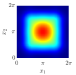
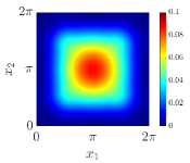
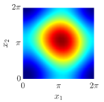
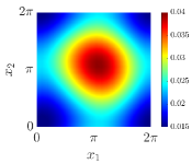
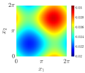
Figure 6: Marginal probability density function (64) obtained by integrating numerically the Fokker–Planck equation (57) in dimension $d=4$ with $\sigma=5$ and initial condition (63) with two methods: i) rank-adaptive implicit step-truncation Euler and ii) rank-adaptive implicit step-truncation midpoint. The reference solution is a variable time step RK4 method with absolute tolerance of $10^{-14}$. These solutions are computed on a grid with $20\times 20\times 20\times 20$ interior points (evenly spaced). The steady state is determined for this computation by halting execution when $\left\|\partial f_{\text{ref}}/\partial t\right\|_{2}$ is below a numerical threshold of $10^{-8}$. This happens at approximately $t\approx 10$ for the initial condition (63).

          Transient Error                                                           Maximal Rank

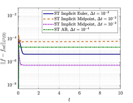
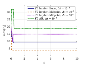
Figure 7: $L^{2}(\Omega)$ error and rank versus time for numerical solutions of Fokker–Planck equation (57) in dimension $d=4$ with initial condition (63). The rank plotted here is the largest rank for all tensors being used to represent the solution in HT format. Rank of the reference solution is in HT format.

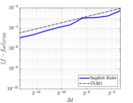
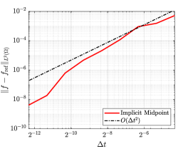
Figure 8: $L^{2}(\Omega)$ errors at $t=0.1$ for the implicit rank-adaptive step-truncation implicit Euler and midpoint methods versus $\Delta t$. The reference solution of (57) if computed using a variable time step RK4 method with absolute tolerance of $10^{-14}$.

Consider the Fokker-Planck equation

$$\frac{{\partial}f({\bm{x}},t)}{\partial t}=-\sum_{i=1}^{d}\frac{\partial}{\partial x_{i}}\left(\mu_{i}({\bm{x}})f({\bm{x}},t)\right)+\frac{\sigma^{2}}{2}\sum_{i=1}^{d}\frac{\partial^{2}f({\bm{x}},t)}{\partial x_{i}^{2}}$$ (57)

on a four-dimensional ($d=4$) flat torus $\Omega=[0,2\pi]^{4}$. The components of the drift are chosen as

$$\mu_{i}({\bm{x}})=(\gamma(x_{i+1})-\gamma(x_{i-2}))\xi(x_{i-1})-\phi(x_{i}),\qquad i=1,\ldots,d,$$ (58)

where $\gamma(x)=\sin(x)$, $\xi(x)=\exp(\sin(x))+1$, and $\phi(x)=\cos(x)$ are $2\pi$-periodic functions. In (58) we set $x_{i+d}=x_{i}$. For this particular drift field, the right side of (57) can be split into a component tangential to the tensor manifold ${\cal H}_{\bm{r}}$ and a component that is non-tangential as

$$\frac{{\partial}f({\bm{x}},t)}{\partial t}=\sum_{i=1}^{d}\underbrace{\left(-\gamma(x_{i+1})\xi(x_{i-1})\frac{\partial f({\bm{x}},t)}{\partial x_{i}}+\gamma(x_{i-2})\xi(x_{i-1})\frac{\partial f({\bm{x}},t)}{\partial x_{i}}\right)}_{\text{Not tangential}}+$$

$$\underbrace{\left(\frac{\partial}{\partial x_{i}}\phi(x_{i})f({\bm{x}},t)+\frac{\sigma^{2}}{2}\frac{\partial^{2}f({\bm{x}},t)}{\partial x_{i}^{2}}\right)}_{\text{tangential}}.$$ (59)

We solve (59) using an operator splitting method. To this end, we notice that there are $3d$ many terms in the summation above, and therefore we first solve the first $d$ time dependent PDEs which are tangential to the tensor manifold ${\cal H}_{\bm{r}}$, i.e.,

$$\frac{\partial g_{i}}{\partial t}=\frac{\partial}{\partial x_{i}}\phi(x_{i})g_{i}+\frac{\sigma^{2}}{2}\frac{\partial^{2}g_{i}}{\partial x_{i}^{2}},\quad\ i=1,\dots,d.$$ (60)

Then we solve the non-tangential equations in two batches,

$$\frac{\partial u_{j}}{\partial t} =\gamma(x_{i+1})\xi(x_{i-1})\frac{\partial u_{j}}{\partial x_{i}},\quad\ \ j=1,\dots,d$$ (61)

$$\frac{\partial u_{k}}{\partial t} =\gamma(x_{i-2})\xi(x_{i-1})\frac{\partial u_{k}}{\partial x_{i}},\quad\ k=2,\dots,2d.$$ (62)

This yields the first-order (Lie-Trotter) approximation $f({\bm{x}},\Delta t)=u_{2d}({\bm{x}},\Delta t)+O(\Delta t^{2})$. We also use these same list of PDEs for the second-order (Strang) splitting integrator. For each time step in both first- and second-order splitting methods, we terminate the HT/TT-GMRES iterations by setting the stopping tolerance $\varepsilon_{\text{tol}}=10^{-9}$. We set the initial probability density function (PDF) as

$$f_{0}(x_{1},x_{2},x_{3},x_{4})=\frac{1}{F_{0}}\sum_{j=1}^{M}\left(\ \prod_{i=1}^{4}\frac{\sin((2j-1)x_{i}-\pi/2)+1}{2^{2(j-1)}}+\prod_{i=1}^{4}\frac{\exp(\cos(2jx_{i}+\pi))}{2^{2j-1}}\right),$$ (63)

where $F_{0}$ is a normalization constant. This gives an HTucker tensor with rank bounded by $2M$. We set $M=10$ to give ranks bounded by $20$. We discretize (57)-(63) in $\Omega$ with the Fourier pseudospectral collocation method [27] on a tensor product grid with $N=20$ evenly-spaced points along each coordinate $x_{i}$, giving the total number of points $(N+1)^{4}=194481$. This number corresponds to the number of entries in the tensor ${\bm{f}}(t)$ appearing in equation (4). Also, we set $\sigma=5$ in (57).

In Figure (6) we compare a few time snapshots of the marginal PDF

$$f_{12}(x_{1},x_{2})=\int_{0}^{2\pi}\int_{0}^{2\pi}f(x_{1},x_{2},x_{3},x_{4})dx_{3}dx_{4},$$ (64)

we obtained with the rank-adaptive implicit step-truncation Euler and midpoint methods, as well as the reference marginal PDF. The solution very quickly relaxes to nearly uniform by $t=0.1$, then slowly rises to its steady state distribution by $t=10$.

In Figure 7 we study accuracy and rank of the proposed implicit step-truncation methods in comparison with the rank-adaptive explicit Adams-Bashforth (AB) method of order 2 (see [40]). The implicit step-truncation methods use a time step size of $\Delta t=10^{-3}$, while step-truncation AB2 uses a step size of $\Delta t=10^{-4}$. The highest error and lowest rank come from the implicit step-truncation midpoint method with $\Delta t=10^{-2}$. The highest rank and second highest error go to the step-truncation AB2 method, which runs with time step size $10^{-4}$ for stability. This causes a penalty in the rank, since the as the time step is made small, the rank must increase to maintain convergence order (see, e.g., (56) for similar conditions on explicit step-truncation midpoint method) The implicit step-truncation midpoint method performs the best, with error of approximately $10^{-6}$ and rank lower than the step-truncation AB2 method at steady state. Overall, the proposed implicit step-truncation methods perform extremely well on linear problems of this form, especially when the right hand side is explicitly written as a sum of tensor products of one dimensional operators. In Figure (8) we show a plot of the convergence rate of implicit step-truncation Euler and midpoint methods. For this figure, we set $\sigma=2$. The convergence rates are order one and order two respectively, verifying Theorem 1.

5.3 Nonlinear Schrödinger equation

          $\theta=0.1$                                                                  $\theta=0.01$

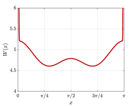
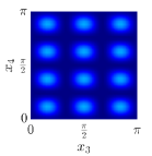
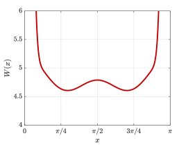
Figure 9: Double-well potential (67)-(68) for different values of $\theta$. It is seen that as $\theta\rightarrow 0$, the potential barrier at $x=0$ and $x=\pi$ becomes infinitely high. This is identical to the well-known homogeneous boundary conditions for particles trapped in a box.

                     $t=0$                                $t=2.5$                                $t=5$

$p(x_{1},x_{2},t)$

$p(x_{3},x_{4},t)$

$p(x_{5},x_{6},t)$

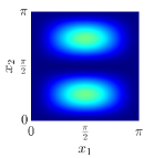
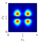
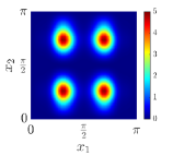
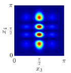
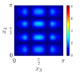
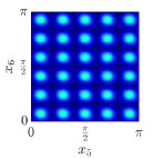
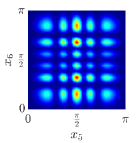
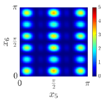
Figure 10: Marginal probability density functions representing particle positions generated by the nonlinear Schrödinger equation (66) with $\varepsilon=10^{-4}$, interaction potential (67) and initial condition (69).

(a)                                                                      (b)

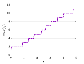
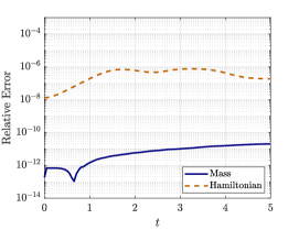
Figure 11: (a) Maximum tensor rank versus time, and (b) relative error in the the solution mass and Hamiltonian (65) for nonlinear Schrödinger equation (66) in dimension $d=6$, with $\varepsilon=10^{-4}$, interaction potential (67) and initial condition (69).

The nonlinear Schrödinger equation is complex-valued PDE whose main applications are wave propagation in nonlinear optical fibers, and Bose-Einstein condensates [44, 42]. The equation can be written as

$$\frac{\partial\phi(\bm{x},t)}{\partial t}=\frac{i}{2}\Delta\phi({\bm{x}},t)-iV({\bm{x}})\phi(\bm{x},t)-i\varepsilon|{\phi}({\bm{x}},t)|^{2}{\phi}({\bm{x}},t).$$ (66)

where $V(\bm{x})$ is the particle interaction potential. In our example, we consider 6 particles trapped on a line segment in the presence of a double-well potential defined as

$$V({\bm{x}})=\sum_{k=1}^{6}W(x_{k}),\qquad W(x_{k})=\left[1+e^{\cos(x_{k})^{2}}+\frac{3}{4}\left(1+e^{\sin(x_{k})^{2}}\right)\right]\eta_{\theta}(x_{k}).$$ (67)

Here, $W(x_{k})$ is a potential with barriers at $x_{k}=0$ and $x_{k}=\pi$ (see Figure 9). The function $\eta_{\theta}(x_{i})$ is a mollifier which converges weakly to $1+\delta(x_{i})+\delta(x_{i}-\pi)$ as $\theta\rightarrow 0$. One such mollifier is

$$\eta_{\theta}(x)=1+\frac{1}{\sqrt{2\pi}\theta}\left(\exp\left[{-\frac{x^{2}}{2\theta^{2}}}\right]+\exp\left[{-\frac{(x-\pi)^{2}}{2\theta^{2}}}\right]\right).$$ (68)

As $\theta\rightarrow 0$, the weak limit of $\eta_{\theta}$ translates to zero Dirichlet boundary conditions on the domain $\Omega=[0,\pi]^{6}$. The Dirichlet conditions naturally allow us to use a discrete sine transform to compute the Laplacian’s differentiation matrices. We discretize the domain $\Omega$ on a uniform grid with 35 points per dimension. This gives us a tensor with $35^{6}=838265625$ entries, or 14.7 Gigabytes per temporal solution snapshot if we store the uncompressed tensor in a double precision IEEE 754 floating point format. We choose a product of pure states for our initial condition, i.e.,

$$\phi({\bm{x}},0)=\prod_{k=1}^{6}\frac{6^{1/6}4k}{2k\pi-\sin(2\pi k)}\sin(kx_{k}),$$ (69)

The normalizing constant $6^{1/6}4k/(2k\pi-\sin(2\pi k))$ guarantees that the wavefunction has an initial mass of 6 particles. We now apply an operator splitting method to solve (66). The linear components are all tangential to the tensor manifold ${\cal H}_{\bm{r}}$, and have a physical interpretation. Specifically,

$$\frac{\partial g_{k}}{\partial t}=\frac{i}{2}\frac{\partial^{2}g_{k}}{\partial x_{k}^{2}}-iW(x_{k})g_{k},\quad\quad k=1,\dots,6,$$ (70)

is a sequence of one-dimensional linear Schrödinger equations. The non-tangential part reduces to

$$\frac{du}{dt}=i\varepsilon|u|^{2}u,$$ (71)

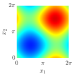
which may be interpreted as an ODE describing all pointwise interactions of the particles. Here we set $\varepsilon=10^{-4}$ to model weak iteractions. Clearly, the linear terms in (66) have purely imaginary eigenvalues. Therefore to integrate the semi-discrete form of (66) in time we need a numerical scheme that has the imaginary axis within its stability region. Since implicit step-truncation Euler method introduces a significant damping, thereby exacerbating inaccuracy due to discrete time stepping, we apply the implicit step-truncation midpoint method. For this problem, we set $\Delta t=5\times 10^{-2}$ and the tensor truncation error to be constant in time at $100\Delta t^{3}$ to maintain second-order consistency. Tolerance of the inexact Newton method was set to $5\times 10^{-5}$ and the HT/TT-GMRES relative error to $5\times\eta=10^{-4}$. In Figure 10 we plot the time-dependent marginal probability density functions for the joint position variables $(x_{k},x_{k+1})$, $k=1,3,5$. Such probability densities are defined as

$$p(x_{1},x_{2},t)=\frac{1}{6}\int_{[0,1]^{4}}\phi^{*}(\bm{x},t)\phi(\bm{x},t){d}x_{3}{d}x_{4}{d}x_{5}{d}x_{6},$$ (72)

and analogously for $p(x_{3},x_{4},t)$ and $p(x_{5},x_{6},t)$. It is seen that the lower energy pure states (position variables $(x_{1},x_{2})$) quickly get trapped in the two wells, oscillating at their bottoms. Interestingly, at $t=2.5$ it appears that particle $x_{3}$ is most likely to be observed in between the two wells whenever the particle $x_{4}$ is in a well bottom.

In Figure 11(a), we plot the rank over time for this problem. The rank also has physical meaning. A higher rank HT tensor is equivalent to a wavefunction with many entangled states, regardless of which $L^{2}(\Omega)$ basis we choose. In the example discussed in this section, the particles interacting over time monotonically increase the rank. We emphasize that the nonlinearity in (66) poses a significant challenge to tensor methods. In fact, in a single application of the function $i\varepsilon|u|^{2}u,$ we may end up tripling the rank. This can be mitigated somewhat by using the approximate element-wise tensor multiplication routine. Even so, if the inexact Newton Method requires many dozens of iterations to halt, the rank may grow very rapidly in a single time step, causing a slowing due to large array storage. This problem is particularly apparent when $\varepsilon\approx 1$ or if $\Delta t$ is made significantly smaller, e.g. $\Delta t=10^{-4}$. A more effective way of evaluating nonlinear functions on tensors decompositions would certainly mitigate this issue. In Figure 11(b), we plot the relative error of the solution mass and the Hamiltonian (65) over time. The relative errors hover around $10^{-11}$ and $10^{-6}$, respectively. It is remarkable that even though the additional tensor truncation done after the inner loop of the implicit solver in principle destroys the symplectic properties of the midpoint method, the mass and Hamiltonian are still preserved with high accuracy.

Appendix A Solving algebraic equations on tensor manifolds

We have seen in section 2 that a large class of implicit step-truncation methods can be equivalently formulated as a root-finding problem for a nonlinear system algebraic equations of the form

$${\bm{H}}({\bm{f}})={\bm{0}}$$ (73)

at each time step. In this appendix we develop numerical algorithms to compute an approximate solution of (73) on a tensor manifold $\mathcal{H}_{\bm{r}}$ with a given rank $\bm{r}$. In other words, we are interested in finding ${\bm{f}}\in\mathcal{H}_{\bm{r}}$ that solves (73) with controlled accuracy. To this end, we combine the inexact inexact Newton method [17, Theorem 2.3 and Corollary 3.5] with the TT-GMRES linear solver proposed in [20].

Theorem 3 (Inexact Newton method [17]).

Let ${\bm{H}}:{\mathbb{R}}^{N}\rightarrow{\mathbb{R}}^{N}$ be continuously differentiable in a neighborhood of a zero $\bm{f}^{*}$, and suppose that the Jacobian of $\bm{H}$, i.e., $\bm{J}_{\bm{H}}(\bm{f})=\partial\bm{H}(\bm{f})/\partial\bm{f}$, is invertible at ${\bm{f}}^{*}$. Given ${\bm{f}}^{[0]}\in{\mathbb{R}}^{N}$, consider the sequence

$${\bm{f}}^{[j+1]}={\bm{f}}^{[j]}+{\bm{s}}^{[j]},\qquad j=0,1,\ldots$$ (74)

where each ${\bm{s}}^{[j]}$ solves the Newton iteration up to relative error $\eta^{[j]}$, i.e., it satisfies

$$\left\|\bm{J}_{\bm{H}}\left({\bm{f}}^{[j]}\right){\bm{s}}^{[j]}+{\bm{H}}\left({\bm{f}}^{[j]}\right)\right\|\leq\left\|{\bm{H}}\left({\bm{f}}^{[j]}\right)\right\|\eta^{[j]}.$$ (75)

If $\eta^{[j]}<1$ for all $j$, then there exists $\varepsilon>0$ so that for any initial guess satisfying $\left\|{\bm{f}}^{[0]}-{\bm{f}}^{*}\right\|<\varepsilon$ the sequence $\{{{\bm{f}}^{[j]}}\}$ converges linearly to ${{\bm{f}}^{[*]}}$. If $\eta^{[j]}\rightarrow 0$ as $j\rightarrow\infty$, then the convergence speed is superlinear.

The next question is how to compute an approximate solution of the linear system

$$\bm{J}_{\bm{H}}\left({\bm{f}}^{[j]}\right){\bm{s}}^{[j]}=-{\bm{H}}\left({\bm{f}}^{[j]}\right)$$ (76)

satisfying the bound (75), without inverting the Jacobian $\bm{J}_{\bm{H}}\left({\bm{f}}^{[j]}\right)$ and assuming that ${\bm{s}}^{[j]}\in\mathcal{H}_{\bm{r}_{j}}$, i.e., that ${\bm{s}}^{[j]}$ is a tensor with rank $\bm{r}_{j}$. To this end we utilize the relaxed HT/TT-GMRES method discussed in [20] HT/TT-GMRES is an adapted tensor-structured generalized minimal residual (GMRES) method to solve linear systems in a tensor format. The solver employs an indirect accuracy check and a stagnation restart check in its halting criterion which we summarize in the following Lemma.

Lemma 1 (Accuracy of HT/TT-GMRES [20]).

Let ${\bm{J}}{\bm{f}}={\bm{b}}$ be a linear system where ${\bm{f}}$, ${\bm{b}}$ are tensors in HT or TT format, and $\bm{J}$ is a bounded linear operator on $\bm{f}$. Let $\{{\bm{f}}^{[0]},{\bm{f}}^{[1]},\ldots\}$ be the sequence of approximate solutions generated by HT/TT-GMRES algorithm in [20], and $\varepsilon>0$ be the stopping tolerance for the iterations. Then

$$\left\|{\bm{J}}{\bm{f}^{[j]}}-{\bm{b}}\right\|\leq m\|{\bm{J}}\|\|{\bm{J}}^{-1}\|\|{\bm{b}}\|\varepsilon,$$ (77)

where $m$ is the number of Krylov iterations performed before restart. Similarly, the distance between ${\bm{f}^{[j]}}$ and the exact solution ${\bm{f}}$ can be bounded as

$$\left\|{\bm{f}^{[j]}}-{\bm{f}}\right\|\leq m\|{\bm{J}}\|\|{\bm{J}}^{-1}\|^{2}\|{\bm{b}}\|\varepsilon.$$ (78)

We can now combine the HT/TT-GMRES linear solver with the inexact Newton method, to obtain an algorithm that allows us to solve nonlinear algebraic equations of the form (73) on a tensor manifold.

Theorem 4 (HT/TT Newton method).

Let ${\bm{H}}:{\mathbb{R}}^{n_{1}\times n_{2}\times\cdots\times n_{d}}\rightarrow{\mathbb{R}}^{n_{1}\times n_{2}\times\cdots\times n_{d}}$ be a continuously differentiable nonlinear map which operates on HT or TT tensor formats, and let ${\bm{f}}^{*}$ be a zero of $\bm{H}$. Suppose that the Jacobian of $\bm{H}$, denoted as $\bm{J}_{\bm{H}}(\bm{f})$, is invertible at $\bm{f}^{*}$. Given an initial guess ${\bm{f}}^{[0]}$, consider the iteration

$${\bm{f}}^{[j+1]}={\mathfrak{T}_{\bm{r}}}\left({\bm{f}}^{[j]}+{\bm{s}}^{[j]}\right)$$ (79)

where ${\bm{s}}^{[j]}$ is the HT/TT-GMRES solution of $\bm{J}_{\bm{H}}\left(\bm{f}^{[j]}\right){\bm{s}}^{[j]}=-{\bm{H}}\left({\bm{f}}^{[j]}\right)$ satisfying

$$\left\|\bm{J}_{\bm{H}}\left(\bm{f}^{[j]}\right){\bm{s}}^{[j]}+{\bm{H}}\left({\bm{f}}^{[j]}\right)\right\|\leq{\frac{1}{2}}\left\|{\bm{H}}\left({\bm{f}}^{[j]}\right)\right\|\eta^{[j]},$$ (80)

where $\eta^{[j]}$ is the relative error, which can be any value in the range $0\leq\eta^{[j]}<1$. Then the Newton iteration converges linearly so long as the rank ${\bm{r}}$ of the truncation operator ${\mathfrak{T}_{\bm{r}}}$ is chosen to satisfy

$$\left\|{\mathfrak{T}_{\bm{r}}}\left({\bm{f}}^{[j]}+{\bm{s}}^{[j]}\right)-{\bm{f}}^{[j]}-{\bm{s}}^{[j]}\right\|\leq\frac{\left\|{\bm{H}}\left({\bm{f}}^{[j]}\right)\right\|}{2\left\|{\bm{J}}^{[j]}\right\|}\eta^{[j]}.$$ (81)

Proof. Let ${\bm{f}}^{[0]}$ be an initial guess. Consider the sequence

$${\bm{\tilde{f}}}^{[j+1]}={\bm{f}}^{[j]}+{\bm{s}}^{[j]}\qquad j=0,1,\ldots$$ (82)

where ${\bm{s}}^{[j]}$ is the HT/TT-GMRES solution of $\bm{J}_{\bm{H}}\left(\bm{f}^{[j]}\right){\bm{s}}^{[j]}=-{\bm{H}}\left({\bm{f}}^{[j]}\right)$ obtained with tolerance

$$\varepsilon_{j}<\frac{\eta^{[j]}}{2m\left\|{\bm{J}}_{\bm{H}}\left(\bm{f}^{[j]}\right)\right\|\left\|{\bm{J}}^{-1}_{\bm{H}}\left(\bm{f}^{[j]}\right)\right\|},$$ (83)

and $0\leq\eta^{[j]}<1$. The next step is to truncate ${\bm{\tilde{f}}}^{[j+1]}$ to a tensor

$${\bm{f}}^{[j+1]}={\mathfrak{T}_{\bm{r}}({\bm{\tilde{f}}}^{[j+1]})}$$ (84)

with rank $\bm{r}$ chosen so that

$$\left\|{\bm{f}}^{[j+1]}-{\bm{\tilde{f}}}^{[j+1]}\right\|<\frac{\left\|{\bm{H}}\left({\bm{f}}^{[j]}\right)\right\|}{2\left\|\bm{J}_{\bm{H}}\left({\bm{f}}^{[j]}\right)\right\|}\eta^{[j]}.$$ (85)

Then the error in solving the Newton iteration this step is

$${\bm{\tilde{r}}}^{[j]}={\bm{J}}_{\bm{H}}\left(\bm{f}^{[j]}\right)\left[{\bm{f}}^{[j+1]}-{\bm{\tilde{f}}}^{[j+1]}+{\bm{s}}^{j}\right]+{\bm{H}}\left({\bm{f}}^{[j]}\right),$$ (86)

which we constructed to satisfy the bound

$$\left\|{\bm{\tilde{r}}}^{[j]}\right\|\leq\left\|{{\bm{J}}_{\bm{H}}\left(\bm{f}^{[j]}\right)}{\bm{s}}^{[j]}+{\bm{H}}\left({\bm{f}}^{[j]}\right)\right\|+\left\|{\bm{J}}_{\bm{H}}\left(\bm{f}^{[j]}\right)\left[{\bm{f}}^{[j+1]}-{\bm{\tilde{f}}}^{[j+1]}\right]\right\|<\left\|{\bm{H}}\left({\bm{f}}^{[j]}\right)\right\|\eta^{[j]}.$$ (87)

Hence, the inexact HT/TT-GMRES Newton method converges linearly. This completes the proof.

∎

An Example

Figure 12: Error versus iteration count of inexact Newton’s method in the HT format.

Let us provide a brief numerical demonstration of the inexact Newton method with HT/TT-GMRES iteration. To this end, consider the cubic function

$$\bm{H}(\bm{f})=1.5{\bm{f}}+0.5{\bm{f}}_{0}+0.125({\bm{f}}+{\bm{f}}_{0})^{3}$$ (88)

where all products are computed using the approximate element-wise Hadamard tensor product with accuracies set to ${10}^{-12}$, and ${\bm{f}}_{0}$ is a given tensor which corresponds to the initial condition used in section 5.1 truncated to an absolute tolerance of $10^{-4}$. The Jacobian operator is easily obtained as

$${\bm{J}}_{\bm{H}}({\bm{f}}){\bm{s}}=1.5{\bm{s}}+0.375({\bm{f}}+{\bm{f}}_{0})^{2}{\bm{s}}.$$ (89)

We set the relative error of the matrix inverse to be $\eta=10^{-3}$. In Figure 12 we plot the results of the proposed inexact Newton method with HT/TT-GMRES iterations. We see that that the target tolerance of $2.2\times 10^{-8}$ is hit in just 12 iterations.

References

• [1] S. M. Allen and J. W. Cahn. Ground state structures in ordered binary alloys with second neighbor interactions. Acta Metall., 20(3):423–433, 1972.
• [2] S. M. Allen and J. W. Cahn. A correction to the ground state of FCC binary ordered alloys with first and second neighbor pairwise interactions. Scripta Metallurgica, 7(12):1261–1264, 1973.
• [3] W. Austin, G. Ballard, and T. G. Kolda. Parallel tensor compression for large-scale scientific data. In IPDPS’16: Proceedings of the 30th IEEE International Parallel and Distributed Processing Symposium, pages 912–922, May 2016.
• [4] M. Bachmayr, R. Schneider, and A. Uschmajew. Tensor networks and hierarchical tensors for the solution of high-dimensional partial differential equations. Found. of Comput. Math., 16(6), 2016.
• [5] J. Baldeaux and M. Gnewuch. Optimal randomized multilevel algorithms for infinite-dimensional integration on function spaces with ANOVA-type decomposition. SIAM J. Numer. Anal., 52(3):1128–1155, 2014.
• [6] V. Barthelmann, E. Novak, and K. Ritter. High dimensional polynomial interpolation on sparse grids. Advances in Computational Mechanics, 12:273–288, 2000.
• [7] M. J. Beran. Statistical continuum theories. New York: Interscience Publishers, 1968.
• [8] A. M. P. Boelens, D. Venturi, and D. M. Tartakovsky. Parallel tensor methods for high-dimensional linear PDEs. J. Comput. Phys., 375:519–539, 2018.
• [9] A. M. P. Boelens, D. Venturi, and D. M. Tartakovsky. Tensor methods for the Boltzmann-BGK equation. J. Comput. Phys., 421:109744, 2020.
• [10] H. J. Bungartz and M. Griebel. Sparse grids. Acta Numerica, 13:147–269, 2004.
• [11] Y. Cao, Z. Chen, and M. Gunzbuger. ANOVA expansions and efficient sampling methods for parameter dependent nonlinear PDEs. Int. J. Numer. Anal. Model., 6:256–273, 2009.
• [12] Y. Chen, L. Zhang, H. Wang, and W. E. Ground state energy functional with Hartree-Fock efficiency and chemical accuracy. J. Phys. Chem. A, 124(35), 2020.
• [13] H. Cho, D. Venturi, and G.E. Karniadakis. Numerical methods for high-dimensional probability density function equations. J. Comput. Phys., 305:817–837, January 2016.
• [14] H. Al Daas, G. Ballard, and P. Benner. Parallel algorithms for tensor train arithmetic. SIAM J. Sci. Comput., 44(1):C25–C53, 2022.
• [15] A. Dektor and D. Venturi. Dynamically orthogonal tensor methods for high-dimensional nonlinear PDEs. J. Comput. Phys., 404:109125, 2020.
• [16] A. Dektor and D. Venturi. Dynamic tensor approximation of high-dimensional nonlinear PDEs. J. Comput. Phys., 437:110295, 2021.
• [17] Ron S. Dembo, Stanley C. Eisenstat, and Trond Steihaug. Inexact newton methods. SIAM Journal on Numerical Analysis, 19(2):400–408, 1982.
• [18] G. Di Marco and L. Pareschi. Numerical methods for kinetic equations. Acta Numerica, 23:369–520, May 2014.
• [19] S. Dolgov, B. Khoromskij, and I. Oseledets. Fast solution of parabolic problems in the tensor train/quantized tensor train format with initial application to the Fokker–Planck equation. SIAM J. Sci. Comput., 34(6):A3016–A3038, 2012.
• [20] S. V. Dolgov. TT-GMRES: solution to a linear system in the structured tensor format. Russian Journal of Numerical Analysis and Mathematical Modelling, 28(2):149–172, 2013.
• [21] W. E, J. Han, and Q. Li. A mean-field optimal control formulation of deep learning. Res. Math. Sci., 6(10):1–41, 2019.
• [22] István Faragó and Agnes Havasiy. Operator splittings and their applications. Nova Science Publishers, 2009.
• [23] J. Foo and G. E. Karniadakis. Multi-element probabilistic collocation method in high dimensions. J. Comput. Phys., 229:1536–1557, 2010.
• [24] L. Grasedyck. Hierarchical singular value decomposition of tensors. SIAM J. Matrix Anal. Appl., 31(4):2029–2054, 2010.
• [25] L. Grasedyck and C. Löbbert. Distributed hierarchical SVD in the hierarchical Tucker format. Numer. Linear Algebra Appl., 25(6):e2174, 2018.
• [26] E. Hairer, C. Lubich, and G. Wanner. Geometric numerical integration, volume 31 of Springer Series in Computational Mathematics. Springer-Verlag, Berlin, second edition, 2006. Structure-preserving algorithms for ordinary differential equations.
• [27] J. S. Hesthaven, S. Gottlieb, and D. Gottlieb. Spectral methods for time-dependent problems. Cambridge University Press, 2007.
• [28] E. Hopf. Statistical hydromechanics and functional calculus. J. Rat. Mech. Anal., 1(1):87–123, 1952.
• [29] A.-K. Kassam and L. N. Trefethen. Fourth-order time stepping for stiff PDEs. SIAM J. Sci. Comput., 26(4):1214–1233, 2005.
• [30] B. N. Khoromskij. Tensor numerical methods for multidimensional PDEs: theoretical analysis and initial applications. In CEMRACS 2013–modelling and simulation of complex systems: stochastic and deterministic approaches, volume 48 of ESAIM Proc. Surveys, pages 1–28. EDP Sci., Les Ulis, 2015.
• [31] E. Kieri and B. Vandereycken. Projection methods for dynamical low-rank approximation of high-dimensional problems. Comput. Methods Appl. Math., 19(1):73–92, 2019.
• [32] D. Kressner and C. Tobler. Algorithm 941: htucker – a Matlab toolbox for tensors in hierarchical Tucker format. ACM Transactions on Mathematical Software, 40(3):1–22, 2014.
• [33] G. Li and H. Rabitz. Regularized random-sampling high dimensional model representation (RS-HDMR). J. Math. Chem., 43(3):1207–1232, 2008.
• [34] L. Li, J. Qiu, and G. Russo. A high order semi-Lagrangian finite difference method for nonlinear Vlasov and BGK models. Comm. Appl. Math. Comput., 5:170–198, 2023.
• [35] H. Montanelli and Y. Nakatsukasa. Fourth-order time-stepping for stiff PDEs on the sphere. SIAM J. Sci. Comput., 40(1):A421–A451, 2018.
• [36] A. Narayan and J. Jakeman. Adaptive Leja sparse grid constructions for stochastic collocation and high-dimensional approximation. SIAM J. Sci. Comput., 36(6):A2952–A2983, 2014.
• [37] M. Raissi and G. E. Karniadakis. Hidden physics models: Machine learning of nonlinear partial differential equations. J. Comput. Phys., 357:125–141, 2018.
• [38] M. Raissi, P. Perdikaris, and G. E. Karniadakis. Physics-informed neural networks: A deep learning framework for solving forward and inverse problems involving nonlinear partial differential equations. J. Comput. Phys., 378:606–707, 2019.
• [39] H. Risken. The Fokker-Planck equation: methods of solution and applications. Springer-Verlag, second edition, 1989. Mathematics in science and engineering, vol. 60.
• [40] A. Rodgers, A. Dektor, and D. Venturi. Adaptive integration of nonlinear evolution equations on tensor manifolds. J. Sci. Comput., 92(39):1–31, 2022.
• [41] A. Rodgers and D. Venturi. Stability analysis of hierarchical tensor methods for time-dependent PDEs. J. Comput. Phys., 409:109341, 2020.
• [42] S. H. Rudy, S. L. Brunton, J. L. Proctor, and J. N. Kutz. Data-driven discovery of partial differential equations. Science Adv., 3(4):e1602614, 2017.
• [43] T. Shi, M. Ruth, and A. Townsend. Parallel algorithms for computing the tensor-train decomposition. ArXiv, (2111.10448):1–23, 2021.
• [44] A. Trombettoni and A. Smerzi. Discrete solitons and breathers with dilute Bose-Einstein condensates. Phys. Rev. Lett., 86:2353–2356, 2001.
• [45] A. Uschmajew. Local convergence of the alternating least squares algorithm for canonical tensor approximation. SIAM J. Matrix Anal. Appl., 33(2):639–652, 2012.
• [46] A. Uschmajew and B. Vandereycken. The geometry of algorithms using hierarchical tensors. Linear Algebra Appl., 439(1):133–166, 2013.
• [47] D. Venturi. The numerical approximation of nonlinear functionals and functional differential equations. Phys. Reports, 732:1–102, 2018.
• [48] D. Venturi and A. Dektor. Spectral methods for nonlinear functionals and functional differential equations. Research in the Mathematical Sciences, 8(27):1–39, 2021.
• [49] Y. Zhu, N. Zabaras, P.-S. Koutsourelakis, and P. Perdikaris. Physics-constrained deep learning for high-dimensional surrogate modeling and uncertainty quantification without labeled data. J. Comput. Phys., 394:56–81, 2019.
• [50] J. Zinn-Justin. Quantum field theory and critical phenomena. Oxford Univ. Press, fourth edition, 2002.