Energy-filtered random-phase states as microcanonical thermal pure quantum states

Abstract

We propose a method to calculate finite-temperature properties of a quantum many-body system for a microcanonical ensemble by introducing a pure quantum state named here an energy-filtered random-phase state, which is also a potentially promising application of near-term quantum computers. In our formalism, a microcanonical ensemble is specified by two parameters, i.e., the energy of the system and its associated energy window. Accordingly, the density of states is expressed as a sum of Gaussians centered at the target energy with its spread corresponding to the width of the energy window. We then show that the thermodynamic quantities such as entropy and temperature are calculated by evaluating the trace of the time-evolution operator and the trace of the time-evolution operator multiplied by the Hamiltonian of the system. We also describe how these traces can be evaluated using random diagonal-unitary circuits appropriate to quantum computation. The pure quantum state representing our microcanonical ensemble is related to a state of the form introduced by Wall and Neuhauser for the filter diagonalization method [M. R. Wall and D. Neuhauser, J. Chem. Phys. 102, 8011 (1995)], and therefore we refer to it as an energy-filtered random-phase state. The energy-filtered random-phase state is essentially a Fourier transform of a time-evolved state whose initial state is prepared as a random-phase state, and the cut-off time in the time-integral for the Fourier transform sets the inverse of the width of the energy window. The proposed method is demonstrated numerically by calculating thermodynamic quantities for the one-dimensional spin-1/2 Heisenberg model on small clusters up to 28 qubits, showing that the method is most efficient for the target energy around which the dense distribution of energy eigenstates is found.

I Introduction

In order to study thermal properties of quantum many-body systems based on the thermodynamic ensembles in statistical mechanics such as the microcanonical, canonical, or grand-canonical ensemble, one might have to calculate the number of microstates, the partition function, or the grand partition function, as their logarithms give the thermodynamic potentials which characterize thermodynamic states. Generally, the microcanonical ensemble formalism is suitable for treating an isolated system, while the canonical or grand canonical ensemble formalism is useful for describing a system coupled to an environment. For quantum many-body systems, these thermodynamic ensembles are expressed by the corresponding density matrices, which are statistical mixtures of pure quantum states Fano (1957). On the other hand, it is often computationally useful to formulate statistical mechanics based directly on pure quantum states, instead of explicitly calculating the density matrices. The pure-state-based approaches make use of the fact that the statistical expectation values of observables are given by the trace of some operators, e.g., a product of the thermal density matrix and an observable. Indeed, the trace can be evaluated without knowing the eigenvalues of these operators. Depending on how the trace is evaluated, the pure-state-based approaches might be classified into two classes.

A well known class of the pure-state-based approach is the purification, where the system size is doubled and the thermal expectation values are calculated as an inner product of pure states in a whole (double-sized) system Fano (1957). In particular, the thermofield-double states Suzuki (1985) are such pure states that are in accordance with the canonical ensemble, implemented for example with the density-matrix-renormalization-group method Feiguin and White (2005) and recently with the variational Monte Carlo method Nomura et al. (2021). It is also worth noting that, given a pure state of a whole system, similarity (or in particular cases equivalence) between the reduced density matrix of a subsystem obtained by bipartitioning the whole system and the thermal density matrix of the subsystem has been recently explored Li and Haldane (2008); Poilblanc (2010); Qi et al. (2012); Dalmonte et al. (2018); Giudici et al. (2018); Mendes-Santos et al. (2020); Seki and Yunoki (2020a).

Another class of the pure-state-based formalism makes use of random states Tolman (1980) to evaluate the trace of observables Drabold and Sankey (1993); Iitaka and Ebisuzaki (2004); Weiße et al. (2006); Jin et al. (2021). In this class, several different methods for the different thermodynamic ensembles have been developed. The methods for the canonical ensemble include the finite-temperature Lanczos method Jaklič and Prelovšek (1994); Prelovšek and Bonča (2013) and the canonical thermal-pure-quantum(TPQ)-state formalism Sugiura and Shimizu (2013). The methods for the microcanonical ensemble include the microcanonical Lanczos method Long et al. (2003); Okamoto et al. (2018) and the TPQ-state formalism Sugiura and Shimizu (2012).

Here, we briefly review state-preparation schemes of the latter class. Let $\hat{\cal H}$ be a Hamiltonian describing the system of interest. In the canonical formalism, for a given inverse temperature $\beta$, a canonical TPQ state is obtained by applying the positive-definite Hermitian operator ${\rm e}^{-\beta\hat{\cal H}/2}$ to a random-phase state, for which either the Lanczos method Jaklič and Prelovšek (1994), the block Lanczos method Seki and Yunoki (2020b), the polynomial-expansion method Weiße et al. (2006), or the Suzuki-Trotter decomposition Suzuki (1990) is often employed. In the microcanonical formalism, for a given energy $E$, the lowest eigenstate of $(\hat{\cal H}-E)^{2}$, which can be obtained via a Lanczos method, is used as a TPQ state in Refs. Long et al. (2003); Okamoto et al. (2018), while the repeated application (i.e., the power iteration) of the properly rescaled Hamiltonian to a random-phase state is used to obtain a TPQ state in Ref. Sugiura and Shimizu (2012).

As compared to the canonical-TPQ-state-preparation schemes, the microcanonical TPQ-state-preparation schemes seem rather indirect in the sense that these methods do not explicitly specify a width of an energy window around a given target energy $E$, which could however be important particularly for finite-size systems where the distribution of the energy eigenvalues is so sparse that the number of microstates depends crucially not only on the target energy $E$ but also on the energy window. Indeed, the width of the energy window in the microcanonical Lanczos method Long et al. (2003) can be estimated from the standard deviation of the energy expectation value with respect to the so-obtained lowest eigenstate of $(\hat{\cal H}-E)^{2}$, thus not being an input parameter, and moreover it does depend on the number of Lanczos iterations. In addition, the power iteration used in the TPQ-state formalism Sugiura and Shimizu (2012) is by construction sequential, starting with a high-energy TPQ state to which the properly rescaled Hamiltonian power is applied as many times as required to reach a TPQ state with a desired energy. While the sequential construction of TPQ states may be advantageous when the thermal properties of the system in the whole energy range are intended to be examined, it is still highly desirable to prepare a TPQ state of an arbitrary target energy with an arbitrary energy window especially when the energy range of interest is limited.

In this paper, we propose a method to calculate finite-temperature properties of many-body systems for a microcanonical ensemble, which may find a potential application of near-term quantum computers. In our formalism, a microcanonical ensemble is specified with a target energy as well as a width of the energy window by expressing the density of states as a sum of Gaussians centered at the target energy with its spread associated with the width of the energy window. Using the Fourier representation of the Gaussian, we can then show that thermodynamic quantities such as entropy and temperature can be calculated by evaluating the trace of the time-evolution operator, which is thus unitary, and the trace of the time-evolution operator multiplied by the Hamiltonian of the system. We also describe how these traces can be evaluated using random diagonal-unitary circuits suitable for quantum computation. The pure state representing our microcanonical ensemble is closely related to a state introduced in the filter-diagonalization method in quantum chemistry Wall and Neuhauser (1995) and thus is named here an energy-filtered random-phase state. The energy-filtered random-phase state is described essentially by the Fourier transform of a time-evolved random-phase state with its dynamics governed by the Hamiltonian of the system and the cut-off time in the time-integral for the Fourier transform is associated with the inverse of the width of the energy window specifying the microcanonical ensemble. We demonstrate the proposed method by numerically calculating thermodynamic quantities of the one-dimensional spin-1/2 Heisenberg model on small clusters and show that the proposed method is most effective for the target energy around which a larger number of energy eigenstates exist.

The rest of this paper is organized as follows. In Sec. II, we define the density of states and, accordingly, the entropy and the inverse temperature that are evaluated from the density of states. In Sec. III, we formulate the proposed method suitable for numerical simulations on classical computers as well as quantum computers. By further examining our formalism as a pure-state approach to a microcanonical ensemble, we show in Sec. IV that the energy-filtered state with an initial random state can be considered as a microcanonical TPQ state. In Sec. V, we introduce a concrete Hamiltonian of the system for the demonstration of the proposed method, and describe the preparation of initial random states and the treatment of the time-evolution operator, both of which are appropriate to quantum computation. In Sec. VI, we demonstrate our proposed method by numerically calculating thermodynamic quantities of the one-dimensional spin-1/2 Heisenberg model up to 28 qubits. Finally, the paper is concluded with discussion in Sec. VII. Additional details on the cumulative number of states, the energy-filtered random-phase state, translation to the canonical ensemble, and the random-phase-product states as well as additional numerical results are provided in Appendixes. Throughout the paper, we set $\hbar=1$ and the Boltzmann constant $k_{B}=1$.

II Preliminaries

In this section, we define the density of states as well as the entropy and the inverse temperature. We also give a few remarks on the choice of the energy window because the number of states within the energy window is a central quantity in the microcanonical ensemble.

II.1 Density of states, entropy, and inverse temperature

Let $\hat{\cal H}$ be the Hamiltonian describing the system of interest on a Hilbert space of dimension $D$, and let $\{E_{n},|E_{n}\rangle\}_{n=0}^{D-1}$ be the eigenpairs of $\hat{\cal H}$ such that $\hat{\cal H}|E_{n}\rangle=E_{n}|E_{n}\rangle$. Without loss of generality, we assume that $E_{0}\leqslant E_{1}\leqslant\cdots\leqslant E_{D-1}$. For given input parameters $E$ and $\tau$, which have the dimensions of energy and time, respectively, we define the density of states $g_{\tau}(E)$ at energy $E$ as

$$g_{\tau}(E)\equiv\frac{\tau}{\sqrt{\pi}}\sum_{n=0}^{D-1}{\rm e}^{-(E_{n}-E)^{2}\tau^{2}}.$$ (1)

It is plausible to call $g_{\tau}(E)$ the density of states because $g_{\tau}(E)$ is reduced to a sum of delta functions in the limit of $\tau\to\infty$ as $\lim_{\tau\to\infty}g_{\tau}(E)=\sum_{n=0}^{D-1}\delta(E_{n}-E),$ which is the conventional form of the density of states. Here, the Gaussian representation of the delta function $\delta(x-\mu)=\lim_{\sigma\to 0}\frac{1}{\sqrt{2\pi}\sigma}{\rm e}^{-\frac{(x-\mu)^{2}}{2\sigma^{2}}}$ is used.

In accordance with the microcanonical ensemble, we define the entropy $S_{\tau}(E)$ as the logarithm of the number of states within a given energy window, i.e.,

$$S_{\tau}(E) \equiv\ln{\left[g_{\tau}(E)\frac{\sqrt{\pi}}{\tau}\right]},$$ (2)

and the inverse temperature $\beta_{\tau}(E)$ as the derivative of $S_{\tau}(E)$ with respect to $E$, i.e.,

$$\beta_{\tau}(E) \equiv\frac{\partial S_{\tau}(E)}{\partial E}=2\tau^{2}\left[{\cal E}_{\tau}(E)-E\right],$$ (3)

where

$${\cal E}_{\tau}(E)\equiv\frac{\sum_{n=0}^{D-1}E_{n}{\rm e}^{-(E_{n}-E)^{2}\tau^{2}}}{\sum_{n=0}^{D-1}{\rm e}^{-(E_{n}-E)^{2}\tau^{2}}}.$$ (4)

We introduced the factor $\frac{\sqrt{\pi}}{\tau}$ in Eq. (2) as the width of the energy window, which makes the argument in the logarithm dimensionless. Hereafter, we refer to $E$ as the target energy and $\tau$ as the filtering time for reasons discussed in Sec. IV.1.

II.2 Trace formalism

Let us introduce a dimensionless positive-definite Hermitian operator

$$\hat{G}_{\tau}(E)\equiv{\rm e}^{-(\hat{\cal H}-E)^{2}\tau^{2}}.$$ (5)

We can then readily show that the density of states, the entropy, and the inverse temperature in Eqs. (1)–(3) are now expressed as

$$g_{\tau}(E) =\frac{\tau}{\sqrt{\pi}}{\rm Tr}\left[\hat{G}_{\tau}(E)\right],$$ (6)

$$S_{\tau}(E) =\ln{\left({\rm Tr}\left[\hat{G}_{\tau}(E)\right]\right)},$$ (7)

and

$$\beta_{\tau}(E) =2\tau^{2}\left(\frac{{\rm Tr}\left[\hat{\cal H}\hat{G}_{\tau}(E)\right]}{{\rm Tr}\left[\hat{G}_{\tau}(E)\right]}-E\right),$$ (8)

respectively. Namely, these quantities are all expressed in terms of ${\rm Tr}\left[\hat{G}_{\tau}(E)\right]$ and ${\rm Tr}\left[\hat{\cal H}\hat{G}_{\tau}(E)\right]$. Therefore, owning to these trace operations, the microscopic energy eigenvalues $\{E_{n}\}_{n=0}^{D-1}$ have ostensibly disappeared in the expressions of the density of states and the thermodynamic quantities $S_{\tau}(E)$ and $\beta_{\tau}(E)$, as it should.

Note that $\hat{\rho}_{\rm mic}\equiv\hat{G}_{\tau}(E)/{\rm Tr}[\hat{G}_{\tau}(E)]$ can be regarded as a density matrix, and a brief consideration on such a Gaussian form of the density matrix, not limited to the microcanonical ensemble, can be found in Ref. Tolman (1980). Moreover, analytical properties of this ensemble have been explored in detail in Refs. Challa and Hetherington (1988); Yoneta and Shimizu (2019). Note also that the energy expectation value in Eq. (4) is expressed as

$${\cal E}_{\tau}(E)=\frac{{\rm Tr}\left[\hat{\cal H}\hat{G}_{\tau}(E)\right]}{{\rm Tr}\left[\hat{G}_{\tau}(E)\right]}={\rm Tr}\left[\hat{\rho}_{\rm mic}\hat{\cal H}\right].$$ (9)

Equations (6)-(9) summarize the density of states, the entropy, the inverse temperature, and the energy expectation value, which are the central quantities considered in this study.

II.3 Energy window and number of states in it

We now make comments on our choice of the width of the energy window, i.e., the factor $\frac{\sqrt{\pi}}{\tau}$ in Eq. (2), and the number of states within the energy window. Approximately, $g_{\tau}(E)\frac{\sqrt{\pi}}{\tau}={\rm Tr}[\hat{G}_{\tau}(E)]=\sum_{n=0}^{D-1}{\rm e}^{-(E_{n}-E)^{2}\tau^{2}}$ in the logarithm of Eqs. (2) and (7) counts the number of energy eigenstates $|E_{n}\rangle$ such that

$$E-\frac{\delta E}{2}\leqslant E_{n}<E+\frac{\delta E}{2},$$ (10)

where $\delta E$ is the width of the energy window here chosen as

$$\delta E=\frac{\sqrt{\pi}}{\tau}.$$ (11)

Based on the dimensional analysis, $1/\tau$ dependence of $\delta E$ is essential, but the factor $\sqrt{\pi}$ in Eq. (11) is not. Here, the factor in $\delta E$ is selected as in Eq. (11) so as for the number of states in the zero-filtering-time limit, i.e., $\tau\to 0$, corresponding to the infinitely large width of the energy window, to satisfy

$$\lim_{\tau\to 0}g_{\tau}(E)\delta E=\lim_{\tau\to 0}{\rm Tr}[\hat{G}_{\tau}(E)]=D,$$ (12)

independently of $E$. In Appendix A, we show that the cumulative number of states is given by a sum of complementary error functions. Finally, we note that $\delta E=\sqrt{\pi}/\tau\,(\sim 1.772/\tau)$ has nothing to do with the “two sigma” $2/\sqrt{2}\tau=\sqrt{2}/\tau\,(\sim 1.414/\tau)$ nor the full width at half maximum (FWHM, $2\sqrt{2\ln 2}\frac{1}{\sqrt{2}\tau}\sim 1.665/{\tau}$) of the Gaussian in Eq. (5).

III Formalism

In this section, we describe how to evaluate ${\rm Tr}[\hat{G}_{\tau}(E)]$ and ${\rm Tr}[\hat{\cal H}\hat{G}_{\tau}(E)]$ without explicitly calculating the energy eigenvalues $\{E_{n}\}_{n=0}^{D-1}$ of the Hamiltonian. In particular, we shall provide a formalism to calculate these quantities by exploiting quantum computers. To this end, we first express $\hat{G}_{\tau}(E)$ in terms of the time-evolution operator, which is thus compatible with quantum computation. We then discuss quantum circuits for the trace evaluation.

III.1 Fourier representation of $\hat{G}_{\tau}(E)$

Since $\hat{G}_{\tau}(E)$ is a Gaussian in the energy domain, it can be expressed by a Fourier transform of a Gaussian in the time domain as

$$\hat{G}_{\tau}(E)=\frac{1}{2\sqrt{\pi}\tau}\int_{-\infty}^{\infty}{\rm d}t\ {\rm e}^{-\frac{t^{2}}{4\tau^{2}}}{\rm e}^{{\rm i}Et}\hat{U}(t),$$ (13)

where

$$\hat{U}(t)\equiv{\rm e}^{-{\rm i}\hat{\cal H}t}$$ (14)

is the time-evolution operator generated by the time-independent Hamiltonian $\hat{\cal H}$. Therefore, ${\rm Tr}[\hat{G}_{\tau}(E)]$ and ${\rm Tr}[\hat{\cal H}\hat{G}_{\tau}(E)]$ can be evaluated by integrating ${\rm Tr}[\hat{U}(t)]$ and ${\rm Tr}[\hat{\cal H}\hat{U}(t)]$ over time $t$, respectively. In the following, we discuss how these traces can be evaluated using random-phase states, which are also suitable for quantum computation.

III.2 Trace evaluation by random sampling

Here, we briefly review the fact that the trace of an operator can be evaluated by taking random average of its diagonal matrix elements of the operator with respect to random-phase states Iitaka and Ebisuzaki (2004), focusing particularly on random-phase states prepared by unitary operators, which is thus compatible with quantum computation, especially, random-diagonal circuits and diagonal-unitary designs Nakata et al. (2014). We also briefly discuss the corresponding variance Jin et al. (2021).

The state called a random-phase state Iitaka and Ebisuzaki (2004) or a phase-random state with equal amplitudes Nakata et al. (2012) has the form of

$$|\Phi_{r}\rangle=\frac{1}{\sqrt{D}}\sum_{b=0}^{D-1}{\rm e}^{{\rm i}\theta_{b,r}}|b\rangle,$$ (15)

where $\{|b\rangle\}_{b=0}^{D-1}$ are the computational-basis states satisfying $\langle b|b^{\prime}\rangle=\delta_{bb^{\prime}}$ and $\sum_{b=0}^{D-1}|b\rangle\langle b|=\hat{I}$, $\{\theta_{b,r}\}_{b=0}^{D-1}$ are random variables drawn uniformly from $[0,2\pi)^{D}$, and $r$ specifies the set of random variables. To be specific, we consider an $N$-qubit system with $D=2^{N}$ and assume that $\{|b\rangle\}_{b=0}^{D-1}$ consists of the eigenstates of Pauli-$Z$ operators. A basis state $|b\rangle$ possesses a bit string of length $N$ associated with the binary representation of $b$. Then, $|\Phi_{r}\rangle$ in Eq. (15) can be written as

$$|\Phi_{r}\rangle=\hat{V}_{r}|+\rangle,$$ (16)

where

$$\hat{V}_{r}\equiv\sum_{b=0}^{D-1}{\rm e}^{{\rm i}\theta_{b,r}}|b\rangle\langle b|$$ (17)

is a diagonal-unitary operator and

$$|+\rangle\equiv\hat{H}^{\otimes N}|0\rangle^{\otimes N}=\frac{1}{\sqrt{D}}\sum_{b=0}^{D-1}|b\rangle$$ (18)

with $\hat{H}$ being the Hadamard gate such that $\hat{H}|0\rangle=\frac{1}{\sqrt{2}}(|0\rangle+|1\rangle)$. Here, $|0\rangle$ ($|1\rangle$) is the eigenstate of the Pauli-$Z$ operator with eigenvalue $+1$ ($-1$).

We can now relate the trace operation and the random average (also see Ref. Iitaka and Ebisuzaki (2004)). Let us consider the random average of some quantity $O_{r}$, which is a functional of the random diagonal-unitary operators $\hat{V}_{r}$ and $\hat{V}_{r}^{\dagger}$, and denote it as

$$\langle\langle O_{r}\rangle\rangle_{R}=\frac{1}{R}\sum_{r=1}^{R}O_{r}.$$ (19)

where $R$ is the number of samples. Note that $O_{r}$ can be either a c-number or an operator. The ideal (i.e., $R\to\infty$) random average of $O_{r}$ is given as

$$\mathbb{E}_{D}[O_{r}] \equiv\lim_{R\to\infty}\langle\langle O_{r}\rangle\rangle_{R}$$

$$=\frac{1}{(2\pi)^{D}}\int_{0}^{2\pi}{\rm d}\theta_{0,r}\int_{0}^{2\pi}{\rm d}\theta_{1,r}\cdots\int_{0}^{2\pi}{\rm d}\theta_{D-1,r}O_{r},$$ (20)

where the second line follows from the assumption that $\{\theta_{b,r}\}_{b=0}^{D-1}$ are drawn uniformly from $[0,2\pi)^{D}$. The subscript $D$ in $\mathbb{E}_{D}$ is to indicate that the number of random variables is $D$. It then follows that the ideal random average of the diagonal matrix element $A_{r}\equiv\langle+|V_{r}^{\dagger}\hat{A}V_{r}|+\rangle$ of operator $\hat{A}$ can be given in terms of ${\rm Tr}[\hat{A}]$, i.e.,

$$\mathbb{E}_{D}\left[A_{r}\right] =\frac{1}{D}\sum_{b^{\prime}=0}^{D-1}\sum_{b=0}^{D-1}\langle b^{\prime}|\hat{A}|b\rangle\mathbb{E}_{D}\left[{\rm e}^{-{\rm i}(\theta_{b^{\prime},r}-\theta_{b,r})}\right]$$

$$=\frac{1}{D}{\rm Tr}\left(\hat{A}\right).$$ (21)

Here, the second equality follows from the identity

$$\mathbb{E}_{D}\left[{\rm e}^{-{\rm i}(\theta_{b^{\prime},r}-\theta_{b,r})}\right]=\delta_{bb^{\prime}}.$$ (22)

This proves the statement described at the beginning of this section.

It is also important to understand how the variance is converged when the trace is evaluated by the random samplings. Since a product of four random-phase factors satisfies the following identity Nakata et al. (2012); Jin et al. (2021):

$$\mathbb{E}_{D}\left[{\rm e}^{-{\rm i}\left(\theta_{i,r}-\theta_{j,r}-\theta_{k,r}+\theta_{l,r}\right)}\right]=\delta_{ij}\delta_{kl}+\delta_{ik}\delta_{jl}-\delta_{ij}\delta_{jk}\delta_{kl},$$ (23)

we can show that the covariance between $A_{r}=\langle\Phi_{r}|\hat{A}|\Phi_{r}\rangle$ and $B_{r}^{*}=\langle\Phi_{r}|\hat{B}^{\dagger}|\Phi_{r}\rangle$ for operators $\hat{A}$ and $\hat{B}$ is given by

$$\mathbb{E}_{D}\left[A_{r}B_{r}^{*}\right]-\mathbb{E}_{D}\left[A_{r}\right]\mathbb{E}_{D}\left[B_{r}^{*}\right]$$

$$= \frac{1}{D^{2}}\left\{\sum_{i,j,k,l}\mathbb{E}_{D}\left[{\rm e}^{-{\rm i}\left(\theta_{i,r}-\theta_{j,r}-\theta_{k,r}+\theta_{l,r}\right)}\right]A_{ij}B_{kl}^{*}-{\rm Tr}\left(\hat{A}\right){\rm Tr}\left(\hat{B}\right)^{*}\right\}$$

$$= \frac{1}{D^{2}}\left[{\rm Tr}\left(\hat{A}\hat{B}^{\dagger}\right)-\sum_{i=0}^{D-1}A_{ii}B_{ii}^{*}\right],$$ (24)

where $A_{ij}=\langle i|\hat{A}|j\rangle$ and $B_{kl}^{*}=\langle l|\hat{B}^{\dagger}|k\rangle=\langle k|\hat{B}|l\rangle^{*}$ are the matrix elements of $\hat{A}$ and $\hat{B}^{\dagger}$ in the computational basis states $|i\rangle$, $|j\rangle$, $|k\rangle$, and $|l\rangle$. Notice in Eq. (24) that the covariance depends on the computational basis used. If $\hat{A}$ and $\hat{B}$ are Hermitian, then the covariance is real. Moreover, when $\hat{B}=\hat{A}$, Eq. (24) is reduced to the variance of $A_{r}$. Most remarkably, the (co)variance decreases exponentially in $N$ as $\sim 1/D=1/2^{N}$, assuming that the numerator in Eq. (24) is $O(D)$.

III.3 Diagonal-unitary $t$-designs for trace evaluation

In order to represent the diagonal unitary $\hat{V}_{r}$ in Eq. (17) on a quantum circuit composed of one- and two-qubit gates, an exponentially large number of gates is required as it contains $D\,(=2^{N})$ random variables. This implies that the preparation of the random-phase state $|\Phi_{r}\rangle$ in Eq. (16) becomes exponentially difficult with increasing $N$. However, as we shall show in this section, we can apply diagonal-unitary $t$-designs Nakata et al. (2014) with $t\geqslant 1$ for the trace evaluation and with $t\geqslant 2$ for the same purpose with exponentially small (co)variance, which therefore avoid such difficulty.

In order to connect the trace evaluation with the diagonal-unitary $t$-design, let us express the state in the form of a density matrix. Namely, by substituting the identity $\langle+|\hat{V}_{r}^{\dagger}\hat{A}\hat{V}_{r}|+\rangle={\rm Tr}\left[\hat{V}_{r}|+\rangle\langle+|\hat{V}_{r}^{\dagger}\hat{A}\right]$ into Eq. (21), we obtain

$${\rm Tr}\left(\hat{A}\right)=D{\rm Tr}\left(\mathbb{E}_{D}\left[\hat{V}_{r}|+\rangle\langle+|\hat{V}_{r}^{\dagger}\right]\hat{A}\right).$$ (25)

It also follows directly from Eq. (22) that the ideal random average maps the pure state $\hat{V}_{r}|+\rangle\langle+|\hat{V}_{r}^{\dagger}$ to the maximally mixed state, i.e.,

$$\mathbb{E}_{D}\left[\hat{V}_{r}|+\rangle\langle+|\hat{V}_{r}^{\dagger}\right]=\frac{\hat{I}}{D},$$ (26)

which indeed satisfies Eq. (25).

The property in Eq. (26) is not unique to the random-phase states of the form $\hat{V}_{r}|+\rangle$, and there are varieties of random states which have a property that its random average gives the maximally mixed state Tolman (1980). Now, we seek for states that can be obtained by replacing the diagonal unitary $\hat{V}_{r}$ with some much simpler unitary $\hat{v}_{r}$ satisfying

$$\mathbb{E}_{N_{v}}\left[\hat{v}_{r}|+\rangle\langle+|\hat{v}_{r}^{\dagger}\right]=\frac{\hat{I}}{D},$$ (27)

so that $\hat{v}_{r}$ can be implemented efficiently on quantum computers. Here, $N_{v}$ is the number of random variables $\{\theta_{k,r}\}_{k=0}^{N_{v}-1}$ in the unitary $\hat{v}_{r}$, and $\mathbb{E}_{N_{v}}$ denotes the corresponding ideal random average. As per the definitions of the $\epsilon$-approximate unitary $t$-designs and of the $\epsilon$-approximate state $t$-designs in Ref. Nakata et al. (2014), it suffices for the trace evaluation that $\hat{v}_{r}$ is a (diagonal-)unitary $t$-design with $t\geqslant 1$.

However, in practical simulations using either classical computers or quantum computers, the number $R$ of samples should be finite. This implies that the states after sampling $\hat{V}_{r}|+\rangle$ and $\hat{v}_{r}|+\rangle$, i.e., $\hat{\rho}_{V_{r}|+\rangle,R}\equiv\frac{1}{R}\sum_{r=1}^{R}[\hat{V}_{r}|+\rangle\langle+|\hat{V}_{r}^{\dagger}]$ and $\hat{\rho}_{v_{r}|+\rangle,R}\equiv\frac{1}{R}\sum_{r=1}^{R}[\hat{v}_{r}|+\rangle\langle+|\hat{v}_{r}^{\dagger}]$, respectively, are in general different from each other and also from their limits $\lim_{R\to\infty}\hat{\rho}_{V_{r}|+\rangle,R}=\lim_{R\to\infty}\hat{\rho}_{v_{r}|+\rangle,R}=\hat{I}/D$ (also see Ref. Iwaki and Hotta (2022) for a related discussion). Therefore, the unitary $\hat{v}_{r}$ selected can affect statistical errors of the random sampling for finite $R$, even if it satisfies Eq. (27). Indeed, as we shall discuss in Sec. VI along with numerical results, (diagonal-)unitary $t$-designs with $t\geqslant 2$ Dankert et al. (2009) are required to suppress statistical errors. Concrete examples of the unitary $\hat{v}_{r}$ related to the diagonal-unitary $t$-design with $t=1$ and $2$ will be given in Sec. V.2.

III.4 Summary of formulation

Here, we summarize the formalism that is suitable for quantum computation. As in Eqs. (6)–(8), we have expressed the density of states $g_{\tau}(E)$, the entropy $S_{\tau}(E)$, and the inverse temperature $\beta_{\tau}(E)$ in terms of ${\rm Tr}[\hat{G}_{\tau}(E)]$ and ${\rm Tr}[\hat{\cal H}\hat{G}_{\tau}(E)]$. With random sampling, ${\rm Tr}[\hat{G}_{\tau}(E)]$ and ${\rm Tr}[\hat{\cal H}\hat{G}_{\tau}(E)]$ can now be evaluated as

$${\rm Tr}[\hat{G}_{\tau}(E)]=\frac{D}{2\sqrt{\pi}\tau}\int_{-\infty}^{\infty}{\rm d}t\ {\rm e}^{-\frac{t^{2}}{4\tau^{2}}}{\rm e}^{{\rm i}Et}\mathbb{E}_{N_{v}}\left[K_{r}(t)\right],$$ (28)

and

$${\rm Tr}[\hat{\cal H}\hat{G}_{\tau}(E)]=\frac{D}{2\sqrt{\pi}\tau}\int_{-\infty}^{\infty}{\rm d}t\ {\rm e}^{-\frac{t^{2}}{4\tau^{2}}}{\rm e}^{{\rm i}Et}\mathbb{E}_{N_{v}}\left[L_{r}(t)\right],$$ (29)

respectively. Here, $K_{r}(t)$ and $L_{r}(t)$ are matrix elements of $\hat{U}(t)$ and $\hat{\cal H}\hat{U}(t)$ defined as

$$K_{r}(t)\equiv\langle+|\hat{v}_{r}^{\dagger}\hat{U}(t)\hat{v}_{r}|+\rangle$$ (30)

and

$$L_{r}(t)\equiv\langle+|\hat{v}_{r}^{\dagger}\hat{\cal H}\hat{U}(t)\hat{v}_{r}|+\rangle,$$ (31)

respectively. Unlike $\hat{V}_{r}$, the unitary $\hat{v}_{r}$ can be implemented efficiently on a quantum computer.

Assuming that we know a form of $\hat{\cal H}$ composed of a linear combination of unitary operators, an example being given later in Eq. (57), the matrix elements $K_{r}(t)$ and $L_{r}(t)$ can be estimated efficiently using quantum computers. Since $K_{r}(-t)=K_{r}(t)^{*}$ and $L_{r}(-t)=L_{r}(t)^{*}$, it is sufficient to evaluate $K_{r}(t)$ and $L_{r}(t)$ only for $t\geqslant 0$ for estimating ${\rm Tr}[\hat{G}_{\tau}(E)]$ and ${\rm Tr}[\hat{\cal H}\hat{G}_{\tau}(E)]$ in Eqs. (28) and (29), respectively. However, in practice, the ideal random averages $\mathbb{E}_{N_{v}}\left[K_{r}(t)\right]$ and $\mathbb{E}_{N_{v}}\left[L_{r}(t)\right]$ in Eqs. (28) and (29), respectively, should be replaced with the random averages $\langle\langle K_{r}(t)\rangle\rangle_{R}$ and $\langle\langle L_{r}(t)\rangle\rangle_{R}$ with a finite number $R$ of samples. Namely, by defining

$${\cal N}_{\tau,r}(E)\equiv\frac{1}{2\sqrt{\pi}\tau}\int_{-\infty}^{\infty}{\rm d}t\ {\rm e}^{-\frac{t^{2}}{4\tau^{2}}}{\rm e}^{{\rm i}Et}K_{r}(t)$$ (32)

and

$${\cal H}_{\tau,r}(E)\equiv\frac{1}{2\sqrt{\pi}\tau}\int_{-\infty}^{\infty}{\rm d}t\ {\rm e}^{-\frac{t^{2}}{4\tau^{2}}}{\rm e}^{{\rm i}Et}L_{r}(t),$$ (33)

we approximate ${\rm Tr}[\hat{G}_{\tau}(E)]$ and ${\rm Tr}[\hat{\cal H}\hat{G}_{\tau}(E)]$ respectively as

$${\rm Tr}[\hat{G}_{\tau}(E)] \approx D\langle\langle{\cal N}_{\tau,r}(E)\rangle\rangle_{R}$$ (34)

and

$${\rm Tr}[\hat{\cal H}\hat{G}_{\tau}(E)] \approx D\langle\langle{\cal H}_{\tau,r}(E)\rangle\rangle_{R}.$$ (35)

Accordingly, the density of states $g_{\tau}(E)$, the entropy $S_{\tau}(E)$, and the inverse temperature $\beta_{\tau}(E)$ in Eqs. (6)–(8) are approximated by those truncated at a finite number $R$ of samples, denoted as $g_{\tau,R}(E)$, $S_{\tau,R}(E)$, and $\beta_{\tau,R}(E)$, respectively:

$$g_{\tau,R}(E) \equiv\frac{\tau}{\sqrt{\pi}}D\langle\langle{\cal N}_{\tau,r}(E)\rangle\rangle_{R},$$ (36)

$$S_{\tau,R}(E) \equiv\ln{\left[D\langle\langle{\cal N}_{\tau,r}(E)\rangle\rangle_{R}\right]},$$ (37)

and

$$\beta_{\tau,R}(E) \equiv 2\tau^{2}\left[{\cal E}_{\tau,R}(E)-E\right],$$ (38)

where

$${\cal E}_{\tau,R}(E)\equiv\frac{\langle\langle{\cal H}_{\tau,r}(E)\rangle\rangle_{R}}{\langle\langle{\cal N}_{\tau,r}(E)\rangle\rangle_{R}}.$$ (39)

These quantities necessarily acquire statistical errors. Obviously, in the limit of $R\to\infty$, $g_{\tau,R}(E)$, $S_{\tau,R}(E)$, $\beta_{\tau,R}(E)$, and ${\cal E}_{\tau,R}(E)$ are reproduced to $g_{\tau}(E)$, $S_{\tau}(E)$, $\beta_{\tau}(E)$, and ${\cal E}_{\tau}(E)$, respectively. Equations (36)–(39) are the central equations of this study, corresponding to Eq. (6)–(9), and these are appropriate to simulations using quantum computers (as well as classical computers).

IV Energy-filtered random-phase state as a TPQ state

In this section, we shall discuss a connection between the formalism developed in Sec. III and a state introduced in the filter-diagonalization method Wall and Neuhauser (1995). While the equations summarized in Sec. III.4 suffice for numerical simulations, the reformulation based on an energy-filtered state allows us to recognize the proposed method as a microcanonical counterpart of the canonical TPQ-state formalism Sugiura and Shimizu (2013).

IV.1 Energy-filtered random-phase state

Let $|\phi_{r}\rangle$ be a normalized random-phase state suitable for the trace evaluation, e.g., $|\phi_{r}\rangle=\hat{v}_{r}|+\rangle$ or $|\phi_{r}\rangle=\hat{V}_{r}|+\rangle$. It follows from Eq. (5) that the positive square root of $\hat{G}_{\tau}(E)$ is given by

$$\left[\hat{G}_{\tau}(E)\right]^{\frac{1}{2}}={\rm e}^{-\frac{1}{2}(\hat{\cal H}-E)^{2}\tau^{2}}=\hat{G}_{\frac{\tau}{\sqrt{2}}}(E).$$ (40)

Let us now introduce an unnormalized state $|\psi_{\tau,r}(E)\rangle$ defined as

$$|\psi_{\tau,r}(E)\rangle \equiv\left[\hat{G}_{\tau}(E)\right]^{\frac{1}{2}}|\phi_{r}\rangle.$$ (41)

Using the Fourier representation for $\hat{G}_{\frac{\tau}{\sqrt{2}}}(E)$ [see Eq. (13)], we can readily show that the state $|\psi_{\tau,r}(E)\rangle$ introduced above can be written as

$$|\psi_{\tau,r}(E)\rangle=\frac{1}{\sqrt{2\pi}\tau}\int_{-\infty}^{\infty}{\rm d}t\ {\rm e}^{-\frac{t^{2}}{2\tau^{2}}}{\rm e}^{{\rm i}Et}\hat{U}(t)|\phi_{r}\rangle.$$ (42)

It is now clear that the state $|\psi_{\tau,r}(E)\rangle$ is essentially a Fourier transform of the time-evolved state $|\phi_{r}(t)\rangle\equiv\hat{U}(t)|\phi_{r}\rangle$ from the initial random state $|\phi_{r}\rangle$, but the interval of the time integral is effectively cut-off around the filtering time $|t|\sim\tau$ by the Gaussian in the integrand. Here we call $|\psi_{\tau,r}(E)\rangle$ an energy-filtered random-phase state. The state of the form in Eq. (42) is originally introduced in a different context to extract eigenvalues and eigenstates of $\hat{H}$ at any desired energy range around a given energy $E$, known as the filter-diagonalization method Wall and Neuhauser (1995).

To examine the properties of the energy-filtered random-phase state $|\psi_{\tau,r}(E)\rangle$, let us expand the initial state $|\phi_{r}\rangle$ by the energy eigenstates as

$$|\phi_{r}\rangle=\sum_{n=0}^{D-1}c_{n,r}|E_{n}\rangle,$$ (43)

where $\{c_{n,r}\}_{n=0}^{D-1}=\{\langle E_{n}|\phi_{r}\rangle\}_{n=0}^{D-1}$ are complex coefficients satisfying the normalization condition $\langle\phi_{r}|\phi_{r}\rangle=\sum_{n=0}^{D-1}|c_{n,r}|^{2}=1$. By substituting Eq. (43) to Eq. (41), we obtain

$$|\psi_{\tau,r}(E)\rangle =\sum_{n=0}^{D-1}{\rm e}^{-\frac{1}{2}(E_{n}-E)^{2}\tau^{2}}c_{n,r}|E_{n}\rangle.$$ (44)

At finite $\tau$, the energy-filtered state is a linear combination of the energy eigenstates whose eigenvalues are concentrated around $E$ with a spread of $\sim\frac{1}{\tau}$. In the zero-filtering-time limit (i.e., $\tau\to 0$), the energy-filtered state coincides with the initial state,

$$\lim_{\tau\to 0}|\psi_{\tau,r}(E)\rangle=|\phi_{r}\rangle.$$ (45)

In the infinite-filtering-time limit (i.e., $\tau\to\infty$), the energy-filtered state multiplied by $\frac{\tau}{\sqrt{2\pi}}$ can be formally written as a linear combination of energy eigenstates weighted by delta functions,

$$\lim_{\tau\to\infty}\frac{\tau}{\sqrt{2\pi}}|\psi_{\tau,r}(E)\rangle =\sum_{n=0}^{D-1}\delta(E-E_{n})c_{n,r}|E_{n}\rangle$$

$$=\delta(E-\hat{H})|\phi_{r}\rangle.$$ (46)

These observations rationalize calling $E$ the target energy and $\tau$ the filtering time. It should be emphasized that, unlike Eq. (45), Eq. (46) is merely a formal expression and $\lim_{\tau\to\infty}|\psi_{\tau,r}(E)\rangle$ is not in practical use.

IV.2 Squared norm and expectation value of the Hamiltonian

In terms of the energy-filtered random-phase state $|\psi_{\tau,r}(E)\rangle$, ${\rm Tr}[\hat{G}_{\tau}(E)]$ and ${\rm Tr}[\hat{\cal H}\hat{G}_{\tau}(E)]$ can be expressed simply as

$${\rm Tr}[\hat{G}_{\tau}(E)] =D\mathbb{E}_{N_{v}}\left[\langle\psi_{\tau,r}(E)|\psi_{\tau,r}(E)\rangle\right]$$ (47)

and

$${\rm Tr}[\hat{\cal H}\hat{G}_{\tau}(E)] =D\mathbb{E}_{N_{v}}\left[\langle\psi_{\tau,r}(E)|\hat{\cal H}|\psi_{\tau,r}(E)\rangle\right],$$ (48)

where the Hermiticity of $[\hat{G}_{\tau}(E)]^{\frac{1}{2}}$ and the identity $\hat{\cal H}\hat{G}_{\tau}(E)=[\hat{G}_{\tau}(E)]^{\frac{1}{2}}\hat{\cal H}[\hat{G}_{\tau}(E)]^{\frac{1}{2}}$ are used. The latter follows from the fact that $\hat{G}_{\tau}(E)$ commutes with $\hat{\cal H}$. Equations (47) and (48) indicates that the density of states as well as the thermodynamic quantities such as the entropy and the inverse temperature can be evaluated simply by sampling the squared norm of the energy-filtered random-phase state $|\psi_{\tau,r}(E)\rangle$ and the expectation value of the Hamiltonian with respect to the energy-filtered random-phase state $|\psi_{\tau,r}(E)\rangle$.

It follows from $\langle\psi_{\tau,r}(E)|\psi_{\tau,r}(E)\rangle=\langle\phi_{r}|\hat{G}_{\tau}(E)|\phi_{r}\rangle$ and $\langle\psi_{\tau,r}(E)|\hat{\cal H}|\psi_{\tau,r}(E)\rangle=\langle\phi_{r}|\hat{\cal H}\hat{G}_{\tau}(E)|\phi_{r}\rangle$ that ${\cal N}_{\tau,r}(E)$ and ${\cal H}_{\tau,r}(E)$ defined in Eqs. (32) and (33) are equivalent to the squared norm of $|\psi_{\tau,r}(E)\rangle$ and the expectation value of the Hamiltonian, respectively, i.e.,

$${\cal N}_{\tau,r}(E) =\langle\psi_{\tau,r}(E)|\psi_{\tau,r}(E)\rangle$$ (49)

and

$${\cal H}_{\tau,r}(E) =\langle\psi_{\tau,r}(E)|\hat{\cal H}|\psi_{\tau,r}(E)\rangle.$$ (50)

Since $0<{\rm e}^{-(E_{n}-E)^{2}\tau^{2}}\leqslant 1$, the squared norm ${\cal N}_{\tau,r}(E)=\sum_{n=0}^{D-1}|c_{n,r}|^{2}{\rm e}^{-(E_{n}-E)^{2}\tau^{2}}$ satisfies $0<{\cal N}_{\tau,r}(E)\leqslant 1$, and the equality is achieved when $\tau=0$. In Appendix B, we give another proof of the equivalence between Eqs. (32) and (49) starting with the time-integral form of the energy-filtered random-phase state $|\psi_{\tau,r}(E)\rangle$ in Eq. (42).

IV.3 Energy-filtered random-phase state as a microcanonical counterpart of the canonical TPQ state

Our construction of the energy-filtered random-phase state $|\psi_{\tau,r}(E)\rangle$ in Eq. (41) reveals its formal similarity to the canonical TPQ state Sugiura and Shimizu (2013), as we shall explain in this section. In the microcanonical ensemble, the number of states ${\rm Tr}\left[\hat{G}_{\tau}(E)\right]$ within a given energy window, specified here by $E$ and $\tau$, is the most fundamental quantity. It then follows from the statistical property of the random-phase state $|\phi_{r}\rangle$ in Eq. (27) that the corresponding energy-filtered random-phase state $|\psi_{\tau,r}(E)\rangle$ in Eq. (41) satisfies

$$D\lim_{R\to\infty}\langle\langle|\psi_{\tau,r}(E)\rangle\langle\psi_{\tau,r}(E)|\rangle\rangle_{R} =\hat{G}_{\tau}(E)$$ (51)

and

$$D\lim_{R\to\infty}\langle\langle\,\langle\psi_{\tau,r}(E)|\psi_{\tau,r}(E)\rangle\,\rangle\rangle_{R} ={\rm Tr}\left[\hat{G}_{\tau}(E)\right].$$ (52)

Accordingly, the density matrix can be given as

$$\hat{\rho}_{\tau}(E)\equiv\frac{\hat{G}_{\tau}(E)}{{\rm Tr}\left[\hat{G}_{\tau}(E)\right]}=\frac{\lim_{R\to\infty}\langle\langle|\psi_{\tau,r}(E)\rangle\langle\psi_{\tau,r}(E)|\rangle\rangle_{R}}{\lim_{R\to\infty}\langle\langle\,\langle\psi_{\tau,r}(E)|\psi_{\tau,r}(E)\rangle\,\rangle\rangle_{R}}.$$ (53)

Obviously, $\hat{\rho}_{\tau}(E)$ does not evolve in time because $\hat{G}_{\tau}(E)$ commutes with $\hat{\cal H}$, and hence it is an equilibrium state. It should be emphasized that as opposed to the TPQ-state formalism Sugiura and Shimizu (2012), there is no need to sequentially prepare, for example, a state associated with lower $E$ from a state with higher $E$ because $E$ and $\tau$ are the input parameters in our case.

In the canonical ensemble, the partition function ${\rm Tr}\left[{\rm e}^{-\beta\hat{\cal H}}\right]$ for a given inverse temperature $\beta$ plays a central role, and the corresponding canonical TPQ state is given by $|\beta_{r}\rangle\equiv{\rm e}^{-\beta\hat{\cal H}/2}|\phi_{r}\rangle$ Sugiura and Shimizu (2013). It is then easy to show that the canonical TPQ state $|\beta_{r}\rangle$ satisfies

$$D\lim_{R\to\infty}\langle\langle|\beta_{r}\rangle\langle\beta_{r}|\rangle\rangle_{R} ={\rm e}^{-\beta\hat{\cal H}}$$ (54)

and

$$D\lim_{R\to\infty}\langle\langle\,\langle\beta_{r}|\beta_{r}\rangle\,\rangle\rangle_{R} ={\rm Tr}\left[{\rm e}^{-\beta\hat{\cal H}}\right].$$ (55)

Accordingly, the density matrix is given as

$$\hat{\rho}_{\rm can}(\beta)\equiv\frac{{\rm e}^{-\beta\hat{\cal H}}}{{\rm Tr}\left[{\rm e}^{-\beta\hat{\cal H}}\right]}=\frac{\lim_{R\to\infty}\langle\langle|\beta_{r}\rangle\langle\beta_{r}|\rangle\rangle_{R}}{\lim_{R\to\infty}\langle\langle\,\langle\beta_{r}|\beta_{r}\rangle\,\rangle\rangle_{R}}.$$ (56)

These formal similarities suggest that the energy-filtered random-phase state $|\psi_{\tau,r}(E)\rangle$ in Eq. (41) can be considered as a microcanonical counterpart of the canonical TPQ state $|\beta_{r}\rangle$. In Appendix C, we show how the present microcanonical ensemble can be translated to the canonical ensemble.

V Model and method

V.1 Hamiltonian

The pure-state formalism for the microcanonical ensemble based on the energy-filtered random-phase state proposed here is now validated numerically by examining the spin-1/2 antiferromagnetic Heisenberg model defined by the following Hamiltonian:

$$\hat{\mathcal{H}}=J\sum_{\langle i,j\rangle}\hat{\mathcal{P}}_{ij}.$$ (57)

Here, $J>0$ is the antiferromagnetic exchange interaction, $\langle i,j\rangle$ runs over all nearest-neighbor pairs of qubits $i$ and $j$ connected with the exchange interaction $J$, and $\hat{\mathcal{P}}_{ij}$ is the swap operator that can be written as

$$\hat{\mathcal{P}}_{ij}=\frac{1}{2}\left(\hat{X}_{i}\hat{X}_{j}+\hat{Y}_{i}\hat{Y}_{j}+\hat{Z}_{i}\hat{Z}_{j}+\hat{I}_{i}\hat{I}_{j}\right)$$ (58)

for $i\not=j$ with $\{\hat{X}_{i},\hat{Y}_{i},\hat{Z}_{i}\}$ and $\hat{I}_{i}$ being the Pauli operators and the identity operator acting on the $i$th qubit. We consider the one-dimensional Heisenberg model consisting of $N=$20, 22, 24, and 28 qubits under periodic boundary conditions. Although we specify the target energy $E$ and the system size $N$ (assumed even) for our microcanonical ensemble, we do not specify other Hamiltonian-symmetry-related properties of the system such as the magnetization and the total momentum. Therefore, the dimension of the Hilbert space is given by $D=2^{N}$.

Note that the Hamiltonian in Eq. (57) can be written as $\hat{\cal H}=2J\sum_{\langle i,j\rangle}\hat{\boldsymbol{S}}_{i}\cdot\hat{\boldsymbol{S}}_{j}+\frac{JN_{\rm bond}}{2}$, where $\hat{\boldsymbol{S}}_{i}=\frac{1}{2}(\hat{X}_{i}\ \hat{Y}_{i}\ \hat{Z}_{i})$ is the vector of the spin-1/2 operators acting on the $i$th qubit and $N_{\rm bond}=\sum_{\langle i,j\rangle}$ is the number of bonds, which is given by $N_{\rm bond}=N$ for the one-dimensional system under periodic boundary conditions. This relation is useful when one compares the energy eigenvalues of $\hat{\cal H}$ in Eq. (57) with those of $J\sum_{\langle i,j\rangle}\hat{\boldsymbol{S}}_{i}\cdot\hat{\boldsymbol{S}}_{j}$, which is the form of a Hamiltonian conventionally used for the spin-1/2 Heisenberg model.

V.2 Initial states

As an initial random state for the trace evaluation, we consider the random-phase state $\hat{V}_{r}|+\rangle$ defined in Eq. (16). In our numerical simulation, $\hat{V}_{r}|+\rangle$ is prepared by assigning the random number $\langle b|\hat{V}_{r}|+\rangle={\rm e}^{{\rm i}\theta_{b,r}}/\sqrt{D}$ to the $b$th entry of the corresponding numeral vector [see Eq. (15)]. In addition to $\hat{V}_{r}|+\rangle$, we consider two types of much simpler random-phase states $\hat{v}_{r}|+\rangle$ using single- and two-qubit gates, as described below.

The first type of $\hat{v}_{r}|+\rangle$ is the random-phase-product state Iitaka (2020), which would be one of the simplest examples of $\hat{v}_{r}|+\rangle$. In this case, the unitary $\hat{v}_{r}=\hat{v}_{r}^{(1)}$ is given by a product of single-qubit $Z$ rotations, i.e.,

$$\hat{v}_{r}^{(1)}=\prod_{k=0}^{N-1}\hat{R}_{Z_{k}}(\theta_{k,r}),$$ (59)

where $\hat{R}_{Z_{k}}(\theta_{k,r})={\rm e}^{-{\rm i}\theta_{k,r}\hat{Z}_{k}/2}$ with $\hat{Z}_{k}$ being Pauli-$Z$ operator acting on the $k$th qubit, and $N_{v}=N$. The random variables $\{\theta_{k,r}\}_{k=0}^{N-1}$ are drawn uniformly from $[0,2\pi)^{N_{v}}$. Note that $\hat{v}_{r}^{(1)}|+\rangle$ is a product state having no entanglements between qubits. In Appendix D, we show that the random-phase-product state satisfies Eq. (27). The random-phase-product states are thus sufficient for taking the trace in principle. However, as we shall show explicitly in Sec. VI.3, the convergence of the trace evaluation via the random sampling is rather slow.

As the second type of $\hat{v}_{r}|+\rangle$, we introduce another random diagonal unitary circuits similar to those in Refs. Nakata et al. (2017a, b), $\hat{v}_{r}=\hat{v}_{r}^{(2)}\hat{v}_{r}^{(1)}$, where $\hat{v}_{r}^{(1)}$ is given in Eq. (59) and $\hat{v}_{r}^{(2)}$ consists of all-to-all $N(N-1)/2$ two-qubit gates, i.e.,

$$\hat{v}_{r}^{(2)}=\prod_{i=0}^{N-1}\prod_{j=0}^{i-1}{\rm e}^{-{\rm i}\hat{Z}_{i}\hat{Z}_{j}\theta_{k(ij),r}}.$$ (60)

Here, the number of random variables in $\hat{v}_{r}=\hat{v}_{r}^{(2)}\hat{v}_{r}^{(1)}$ is $N_{v}=N+N(N-1)/2=N(N+1)/2$, and $k(ij)$ in Eq. (60) maps a two-dimensional label $\{ij\}$ to a one-dimensional label $k$ which runs from $N$ to $N(N+1)/2-1$. It is obvious that $\hat{v}_{r}=\hat{v}_{r}^{(2)}\hat{v}_{r}^{(1)}$ also satisfies Eq. (27) because it contains $\hat{v}_{r}^{(1)}$ (see Appendix D), implying that it is also sufficient for the trace evaluation. However, in contrast to $\hat{v}_{r}^{(1)}$, $\hat{v}_{r}^{(2)}$ can apparently generate entanglements between qubits. The random variables $\{\theta_{k,r}\}_{k=0}^{N_{v}-1}$ are drawn uniformly from $[0,2\pi)^{N_{v}}$. Namely, unlike unitary $t$-designs, the random variables are assumed to be continuous here.

V.3 Time-evolution operator

We approximate the time-evolution operator $U(t)$ in Eq. (14) by the first-order Suzuki-Trotter decomposition Trotter (1959); Suzuki (1976) of the form

$$\hat{U}(t)\approx\left[\hat{S}(\Delta_{t})\right]^{M}\equiv\left[{\rm e}^{-{\rm i}\hat{\cal H}_{A}\Delta_{t}}{\rm e}^{-{\rm i}\hat{\cal H}_{B}\Delta_{t}}\right]^{M}$$ (61)

where $M$ is an integer such that $t=M\Delta_{t}$, $\hat{\cal H}_{A}$ ($\hat{\cal H}_{B}$) consists of the Hamiltonian terms acting on the odd (even) bonds, i.e., $\hat{\cal{H}}=\hat{\cal H}_{A}+\hat{\cal H}_{B}$ with $\hat{\cal H}_{A\,(B)}=J\sum_{i:\,{\text{odd (even)}}}\hat{\cal P}_{i,i+1}$, and $\Delta_{t}$ is a small time slice. Accordingly, we discretize the time integrals in Eqs. (32) and (33) with the trapezoidal rule. In our numerical demonstration shown in Sec. VI, we calculate thermodynamic quantities with the filtering time $\tau$ varying $0<\tau J\leqslant 5$. It turns out that taking the range of the time integral over $0\leqslant tJ\leqslant t_{\rm max}J$ (see Sec. III.4) with $t_{\rm max}J=50$, instead of infinity, and $\Delta_{t}J=0.01$ gives quantitatively converged results. We thus set the number $M$ of time slices as large as $M=50/\Delta_{t}J=5000$.

Figure 1 shows schematically a quantum circuit for preparing the time-evolved state $[\hat{S}(\Delta_{t})]^{M}\hat{v}_{r}^{(2)}\hat{v}_{r}^{(1)}|+\rangle$. Here, the “$V$” gate with angle $\theta_{k}$ connecting qubits $i$ and $j$, appearing in the $\hat{v}_{r}^{(2)}$ part of the quantum circuit in the figure, denotes ${\rm e}^{-{\rm i}\hat{Z}_{i}\hat{Z}_{j}\theta_{k,r}}$. Note that the order of quantum gates in the part of the quantum circuit corresponding to the diagonal unitary $\hat{v}_{r}^{(2)}\hat{v}_{r}^{(1)}$ is irrelevant because these quantum gates commute among each other. The “$2\Delta_{t}J$” gate connecting qubits $i$ and $j$ that appears in the $[\hat{S}(\Delta_{t})]^{M}$ part of the quantum circuit in the figure denotes the exponential-SWAP gate ${\rm e}^{-{\rm i}\theta\hat{\cal P}_{ij}/2}$ with angle $\theta=2\Delta_{t}J$ Seki et al. (2020). The matrix element of the time-evolution operator in Eq. (30), here approximated by the Suzuki-Trotter decomposition, i.e.,

$$K_{r}(t)\approx\langle+|\hat{v}_{r}^{(1){\dagger}}\hat{v}_{r}^{(2){\dagger}}[\hat{S}(\Delta_{t})]^{M}\hat{v}_{r}^{(2)}\hat{v}_{r}^{(1)}|+\rangle$$ (62)

can be evaluated with the Hadamard test on quantum computers. For example, the real part of $K_{r}(t)$ can be evaluated with the Hadamard test by adding one ancillary qubit in $|+\rangle_{\rm a}=\frac{1}{\sqrt{2}}(|0\rangle_{\rm a}+|1\rangle_{\rm a})$ (where the subscript “${\rm a}$” indicates the ancillary qubit), replacing the quantum gates for $[\hat{S}(\Delta_{t})]^{M}$ by those for the controlled-$[\hat{S}(\Delta_{t})]^{M}$ gate with the control qubit being the ancillary qubit, and measuring the ancillary qubit in $|+\rangle_{\rm a}$ basis. The imaginary part can be evaluated similarly. In the same manner, the other matrix element in Eq. (31), i.e.,

$$L_{r}(t)\approx J\sum_{\langle ij\rangle}\langle+|\hat{v}_{r}^{(1){\dagger}}\hat{v}_{r}^{(2){\dagger}}\hat{\cal P}_{ij}[\hat{S}(\Delta_{t})]^{M}\hat{v}_{r}^{(2)}\hat{v}_{r}^{(1)}|+\rangle$$ (63)

can also be evaluated with the Hadamard test on quantum computers.

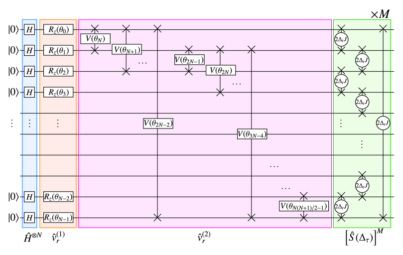
Figure 1: Quantum circuit for preparing the state $[\hat{S}(\Delta_{t})]^{M}\hat{v}_{r}^{(2)}\hat{v}_{r}^{(1)}|+\rangle$. Operator expressions for $\hat{v}_{r}^{(1)}$, $\hat{v}_{r}^{(2)}$, and $[\hat{S}(\Delta_{t})]^{M}$ are given in Eqs. (59), (60), and (61), respectively. In the time-evolution operator part, $[\hat{S}(\Delta_{t})]^{M}$, we assume the one-dimensional Heisenberg model under periodic boundary conditions. Note that the subscript “$r$” in $\theta_{k,r}$ is omitted for simplicity.

VI Numerical results

VI.1 Number of states

In the microcanonical ensemble, the number of states within an energy window at a give energy $E$ plays a central role, because its logarithm corresponds to the entropy, which is the thermodynamic potential in the microcanonical ensemble. We thus first examine how our definition of the number of states within an energy window, $g_{\tau}(E)\delta E$, behaves in the one-dimensional Heisenberg model for $N=$20, 22, and 24. The results for smaller system sizes are also provided in Appendix E.

Figure 2 shows histograms of the number of states. Here, a histogram is made by dividing the energy range $[E_{0},E_{D-1}]$ of the whole energy eigenvalues into $N_{\rm bin}$ number of bins, and hence the height of a bar of a histogram corresponds to the number of states within an energy window $[E-\delta E_{N_{\rm bin}}/2,E+\delta E_{N_{\rm bin}}/2)$, where

$$\delta E_{N_{\rm bin}}\equiv\frac{E_{D-1}-E_{0}}{N_{\rm bin}-1},$$ (64)

and we allocate $N_{\rm bin}$ bins so that the minimum (maximum) energy eigenvalue $E_{0}$ ($E_{D-1}$) is located at the center of the corresponding bin. In Fig. 2, we plot the results for $N_{\rm bin}=32$, 64, and 128. Note that basically the same histogram but with a different $\delta E_{N_{\rm bin}}$ for $N=20$ has already been reported in Ref. Okamoto et al. (2018). For comparison, we also show in the figure the number of states calculated form our definition, i.e.,

$${\rm Tr}\left[\hat{G}_{\tau}(E)\right]=g_{\tau}(E)\delta E,$$ (65)

where $\delta E$ is given in Eq. (11) and the filtering time $\tau$ is chosen as

$$\tau=\frac{\sqrt{\pi}}{\delta E_{N_{\rm bin}}},$$ (66)

hence satisfying $\delta E=\delta E_{N_{\rm bin}}$. More explicitly, the values of $\tau$ are $\tau J=$1.98, 1.80, 1.65 for $N_{\rm bin}=32$ and $N=20,22,24$, $\tau J=$4.02, 3.65, 3.35 for $N_{\rm bin}=64$ and $N=20,22,24$, and $\tau J=$8.09, 7.36, 6.75 for $N_{\rm bin}=128$ and $N=20,22,24$, respectively.

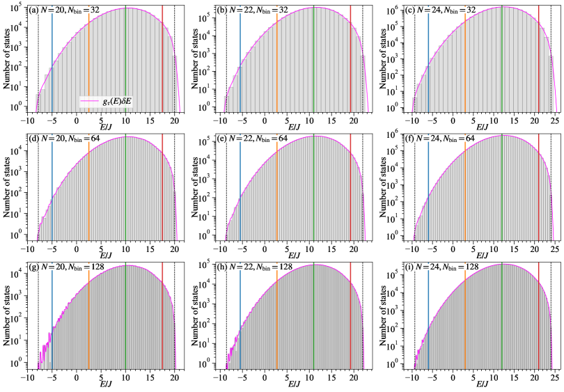
Figure 2: Semilog plots of the histograms for the the number of states as a function of the target energy $E$ with (a,b,c) $N_{\rm bin}=32$, (d,e,f) $N_{\rm bin}=64$, and (g,h,i) $N_{\rm bin}=128$ for (a,d,g) $N=20$, (b,e,h) $N=22$, and (c,f,i) $N=24$. For comparison, the number of states calculated from ${\rm Tr}[\hat{G}_{\tau}(E)]=g_{\tau}(E)\delta E$ with the filtering time $\tau$ chosen as in Eq. (66) is also shown in each panel by the magenta line. The thin dashed vertical lines at the edges of the histograms indicate the minimum and maximum energy eigenvalues $E_{0}$ and $E_{D-1}$. The thick vertical lines at $E/NJ=-0.25,0.125,0.5,$ and $0.875$ (indicated by blue, orange, green, and red, respectively) denote the target energies used in the results shown in Figs. 3, 4, 5, and 11. Notice that the different panels employ the different axes scales.

It is found in Fig. 2 that ${\rm Tr}[\hat{G}_{\tau}(E)]=g_{\tau}(E)\delta E$ closely follows the corresponding histogram of the number of states, indicating that our definitions of the density of states $g_{\tau}(E)$ and the width of the energy window $\delta E$ are reasonable. We note that, in contrast to the histograms, ${\rm Tr}[\hat{G}_{\tau}(E)]=g_{\tau}(E)\delta E$ is a continuous function of $E$ and hence its derivative with respect to $E$ is well defined even for finite-size systems. However, when the energy eigenvalues are distributed sparsely as compared to a given energy window, $g_{\tau}(E)\delta E$ behaves snaky [for example, see a low-energy region in Figs. 2(g)–2(i)] and such a behavior becomes more prominent for the smaller $N$ and the larger $N_{\rm bin}$ (see Fig. 8 in Appendix E). On the other hand, thermodynamically, the entropy $S_{\tau}(E)=\ln[g_{\tau}(E)\delta E]$ should be a concave function of $E$ so that the inverse temperature $\beta_{\tau}(E)=\partial S_{\tau}(E)/\partial E$ decreases monotonically with $E$. This implies that if the filtering time $\tau$ is so large that $\delta E$ is smaller than the energy-eigenvalue spacing at energy around $E$, the statistical mechanical treatment of these quantum states becomes irrelevant and hence loses connections to thermodynamics, as it is usually the case in statistical mechanics. In this sense, the proposed method is expected to be most effective for larger systems where the distribution of the energy eigenvalues is dense.

VI.2 Filtering-time dependence

In the thermodynamic limit, thermodynamic quantities should not depend significantly on the width of the energy window $\delta E=\sqrt{\pi}/\tau$, as long as a large number of energy eigenstates are contained within the energy window $[E-\delta E/2,E+\delta E/2)$, rationalizing the treatment of a microcanonical ensemble. However, for finite-size systems, the width of the energy window affects the results in general. Therefore, here we numerically examine how the energy expectation value ${\cal E}_{\tau}(E)$ in Eq. (9), the entropy $S_{\tau}(E)$ in Eq. (7), the inverse temperature $\beta_{\tau}(E)$ in Eq. (8), and the energy fluctuation depend on the filtering time $\tau$ and thus the width of the energy window $\delta E=\sqrt{\pi}/\tau$. For this purpose, we employ the full diagonalization method to evaluate these quantities numerically exactly without introducing any random sampling. For each system size $N$, four target energies $E/NJ=-0.25,0.125,0.5$, and $0.875$ are selected (see the vertical lines in Fig. 2). Notice that we choose $E$ proportional to $N$ in order to compare the results for different system sizes. The results for smaller system sizes are also provided in Appendix E.

VI.2.1 Energy expectation value

Figures 3(a)-3(c) show the $\tau$ dependence of the energy expectation value ${\cal E}_{\tau}(E)$, which may approach the target energy $E$ with increasing the filtering time $\tau$, as long as there exist energy eigenvalues $\{E_{n}\}$ in the range of Eq. (10). The energy expectation value starts from its value in the zero-filtering-time limit,

$$\lim_{\tau\to 0}{\cal E}_{\tau}(E)=\frac{1}{D}{\rm Tr}\left[\hat{\cal H}\right],$$ (67)

which is in our case reduced simply to $\lim_{\tau\to 0}{\cal E}_{\tau}(E)=JN_{\rm bond}/2$ because ${\rm Tr}[\hat{\boldsymbol{S}}_{i}\cdot\hat{\boldsymbol{S}}_{j}]=0$ for $i\neq j$. As expected, ${\cal E}_{\tau}(E)$ deviates from its zero-filtering-time limit and approaches the target energy $E$ with increasing $\tau$. Moreover, it is interesting to find that ${\cal E}_{\tau}(E)$ as a function of $\tau$ is almost always within the energy window $[E-\delta E/2,E+\delta E/2)$ (indicated with the shaded areas in the figures) with no significant difference for different system sizes [also see Figs. 9(a)–9(c) in Appendix E]. Although we already have the target energy $E$ as an input parameter, the energy expectation value ${\cal E}_{\tau}(E)$ is a useful quantity to check if the filtering time $\tau$ is so large that ${\cal E}_{\tau}(E)$ is consistent with the target energy $E$.

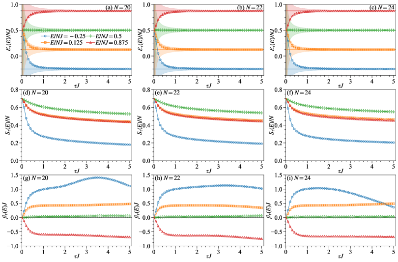
Figure 3: (a,b,c) The energy expectation value ${\cal E}_{\tau}(E)$, (d,e,f) the entropy $S_{\tau}(E)$, and (g,h,i) the inverse temperature $\beta_{\tau}(E)$ as a function of the filtering time $\tau$ for (a,d,g) $N=20$, (b,e,h) $N=22$, and (c,f,i) $N=24$ calculated using the full diagonalization method. In (a,b,c), the horizontal blue, orange, green, and red lines indicate the target energies $E/NJ=-0.25$, $0.125$, $0.5$, and $0.875$, respectively (also see Fig. 2), and the shaded areas indicate the corresponding energy windows $[E-\delta E/2,E+\delta E/2)$. In (d,e,f), the results for $E/NJ=0.125$ (orange) and $E/NJ=0.875$ (red) are almost on top of each other in this scale.

VI.2.2 Entropy

Figures 3(d)-3(f) show the $\tau$ dependence of the entropy $S_{\tau}(E)$. The entropy in the zero-filtering-time limit is given by

$$\lim_{\tau\to 0}S_{\tau}(E)=\ln D,$$ (68)

as explained in Sec. II.3 [see Eq. (12)]. It is also readily shown that the entropy $S_{\tau}(E)$ is a decreasing function of $\tau$, i.e.,

$$\frac{\partial S_{\tau}(E)}{\partial\tau}=\frac{1}{{\rm Tr}\left[\hat{G}_{\tau}(E)\right]}\frac{\partial{\rm Tr}\left[\hat{G}_{\tau}(E)\right]}{\partial\tau}\leqslant 0,$$ (69)

because $\partial_{\tau}{\rm Tr}[\hat{G}_{\tau}(E)]=-2\tau{\sum_{n=0}^{D-1}(E_{n}-E)^{2}{\rm e}^{-(E_{n}-E)^{2}\tau^{2}}}\leqslant 0$ and ${\rm Tr}[\hat{G}_{\tau}(E)]>0$. The inequality in Eq. (69) can be understood intuitively because the number of states in the energy window $[E-\delta E/2,E+\delta E/2)$, which is given by ${\rm Tr}[\hat{G}_{\tau}(E)]$, never increases with decreasing $\delta E$ (also see Fig. 2). The equality in Eq. (69) is achieved when $\tau=0$, and hence the maximum value of the entropy is in the zero-filtering-time limit given in Eq. (68).

Among the four target energies, the difference in the entropy among the different system sizes $N$ is somewhat significant for $E/NJ=-0.25$, for which the larger $N$ has the larger entropy [also see Figs. 9(d)–9(f) in Appendix E]. This behavior is consistent with the results for the number of states shown in Fig. 2, where the energy eigenvalues are distributed rather sparsely around $E/NJ=-0.25$.

VI.2.3 Inverse temperature

Figures 3(g)-3(i) show the $\tau$ dependence of the inverse temperature $\beta_{\tau}(E)$. The inverse temperature starts with its value in the zero-filtering-time limit,

$$\lim_{\tau\to 0}\beta_{\tau}(E)=0,$$ (70)

corresponding to the infinite temperature. At finite $\tau$, $\beta_{\tau}(E)$ can be either positive or negative as it is obvious from Eq. (8). The positive (negative) temperature can be obtained when the energy expectation value ${\cal E}_{\tau}(E)$ is larger (smaller) than the target energy $E$. Indeed, the inverse temperature for $E/NJ=0.5$ remains around 0 even when $\tau$ is increased, and the inverse temperature for the target energy smaller (larger) than $E/NJ=0.5$ (corresponding to the infinite temperature) is positive (negative). This is expected because the slope of the magenta line in Fig. 2 is related to the inverse temperature at the corresponding target energy, i.e., $\beta_{\tau}(E)=\partial_{E}\ln{{\rm Tr}[\hat{G}_{\tau}(E)]}$ from Eqs. (3) and (7).

We also find that for target energies $E/NJ=0.125$, 0.5, and 0.875, around which the distribution of energy eigenstates is dense, the inverse temperature $\beta_{\tau}(E)$ becomes almost independent of $\tau$, i.e.,

$$\frac{\partial\beta_{\tau}(E)}{\partial\tau}\approx 0,$$ (71)

once $\tau$ becomes sufficiently large, i.e., $\tau J\sim 1.0$, where the energy expectation value ${\cal E}_{\tau}(E)$ essentially reaches the target energy $E$, and this almost $\tau$ independent behavior of $\beta_{\tau}(E)$ continues up to $\tau J\lesssim 3$. Moreover, the $\tau$ dependence becomes less significant for larger $N$ [also see Figs. 9(g)–9(i) in Appendix E]. The $\tau$-independent $\beta_{\tau}(E)$ implies that the energy expectation value ${\cal E}_{\tau}(E)$ approaches the target energy $E$ in $\tau$ as $1/\tau^{2}$, i.e., ${\cal E}_{\tau}(E)-E=\beta(E)/2\tau^{2}$, where $\beta(E)$ is a representative value of $\beta_{\tau}(E)$ satisfying the condition in Eq. (71).

On the other hand, the inverse temperature $\beta_{\tau}(E)$ depends rather wildly on $\tau$ for $E/NJ=-0.25$. In particular, the inverse temperature for $N=14$, 16 and 18 becomes negative for $\tau J\gtrsim 4$ [see Figs. 9(g)–9(i) in Appendix E], although a positive value is expected for the target energy smaller than $E/NJ=0.5$. Such a dependence is due to the sparse distribution of energy eigenstates around $E/NJ=-0.25$ (see Figs. 2 and 8). Namely, if $\tau$ is so large that the number of energy eigenstates within the energy window is insufficiently small for considering the microcanonical ensemble, the calculation of thermodynamic quantities fails, as it is well known in statistical mechanics. Finally, we note that except for $E/NJ=-0.25$, the $\tau$-dependence of the inverse temperature is more moderate for $N=24$ than for $N=20$ and 22 because of the denser distribution of energy eigenstates around the target energy $E$. As discussed in Sec. VI.3, this will be more evident for $N=28$ (see Fig. 6), where the full-diagonalization results are not available.

VI.2.4 Energy fluctuation

Figure 4 shows the $\tau$ dependence of the energy fluctuation $\sigma_{\tau}(E)$ defined as

$$\sigma_{\tau}(E)\equiv\sqrt{\frac{{\rm Tr}\left[\hat{\cal H}^{2}\hat{G}_{\tau}(E)\right]}{{\rm Tr}\left[\hat{G}_{\tau}(E)\right]}-{\cal E}_{\tau}(E)^{2}}.$$ (72)

We first notice in the figure that the system-size dependence of $\sigma_{\tau}(E)$ is not significant (also see Fig. 10 in Appendix E). As expected from the Gaussian form of $\hat{G}_{\tau}(E)$ in Eq. (5), we also find that the energy fluctuation for large $\tau$ behaves as

$$\sigma_{\tau}(E)\sim\frac{1}{\sqrt{2}\tau}.$$ (73)

This is because $1/\sqrt{2}\tau$ is the “sigma” of the Gaussian in Eq. (5). However, as opposed to what is expected from the form of $1/\sqrt{2}\tau$, $\sigma_{\tau}(E)$ never diverges for $\tau\to 0$ simply because the energy eigenvalues are distributed only in the finite range of $[E_{0},E_{D-1}]$, and hence $\sigma_{\tau}(E)$ deviates from $1/\sqrt{2}\tau$ for small $\tau$. Finally, we note that the half width of the energy window, $\delta E/2=\sqrt{\pi}/2\tau$, is less relevant for describing the energy fluctuation for large $\tau$.

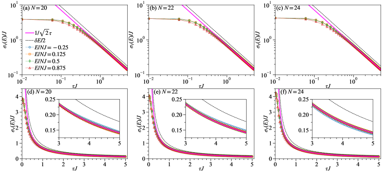
Figure 4: The energy fluctuation $\sigma_{\tau}(E)$ as a function of the filtering time $\tau$ for different target energies $E/NJ=-0.25$, $0.125$, $0.5$, and $0.875$ denoted by blue circles, orange squares, green diamonds, and red triangles, respectively, for (a) $N=20$, (b) $N=22$, and (c) $N=24$ calculated using the full diagonalization method. For comparison, $1/\sqrt{2}\tau$ and $\delta E/2$ are also indicated by thick magenta line and thin black dashed line, respectively. (d-f) show the same results as in (a-c) but plotted in a linear scale. The insets in (d-f) show the magnifications for $3\leqslant\tau J\leqslant 5$.

VI.3 Comparison with random sampling for trace evaluation

The numerical results shown so far have been calculated by fully diagonalizing the Hamiltonian and thus they are free from statistical errors. Now we shall compare these results with those obtained on the basis of the energy-filtered random-phase states with the random sampling for the trace evaluations as in Eqs. (34) and (35). Note that the latter results with the number $R$ of random samples being infinity are essentially identical to the former results obtained by the full diagonalization method. One technical advantage of the random sampling approach is that one can treat larger systems, as we shall also demonstrate here.

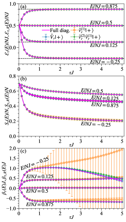
Figure 5: (a) The energy expectation value ${\cal E}_{\tau,R}(E)$, (b) the entropy $S_{\tau,R}(E)$, and (c) the inverse temperature $\beta_{\tau,R}(E)$ as a function of the filtering time $\tau$ for different target energies $E/NJ=-0.25$, $0.125$, $0.5$, and 0.875 calculated with the random sampling of the trace evaluations using three types of the random-phase states, i.e., $\hat{V}_{r}|+\rangle$ (blue circles), $\hat{v}_{r}^{(1)}|+\rangle$ (orange squares), and $\hat{v}_{r}^{(2)}\hat{v}_{r}^{(1)}|+\rangle$ (green diamonds). The system size is fixed at $N=24$ for all the calculations and the number of samples is $R=64$. For comparison, the results for ${\cal E}_{\tau}(E)$, $S_{\tau}(E)$, and $\beta_{\tau}(E)$ calculated by the full diagonalization method are also shown by magenta solid lines. Note that these full-diagonalization results are the same as those in Figs. 3(c), 3(f), and 3(i). The black dashed horizontal lines in (a) indicate the target energies. For most of the cases, the results, including the statistical errors, for $\hat{V}_{r}|+\rangle$ and $\hat{v}_{r}^{(2)}\hat{v}_{r}^{(1)}|+\rangle$ are almost indistinguishable. Moreover, the results in (b) for $E/NJ=0.125$ and $0.875$ are on top of each other in this scale.

Figure 5 shows the results for the energy expectation value ${\cal E}_{\tau,R}(E)$, the entropy $S_{\tau,R}(E)$, and the inverse temperature $\beta_{\tau,R}(E)$ of the $N=24$ system evaluated using the random-phase states $\hat{V}_{r}|+\rangle$, $\hat{v}_{r}^{(1)}|+\rangle$, and $\hat{v}_{r}^{(2)}\hat{v}_{r}^{(1)}|+\rangle$, which are also compared with those for ${\cal E}_{\tau}(E)$, $S_{\tau}(E)$, and $\beta_{\tau}(E)$ obtained by the full diagonalization method. For the trace evaluation with the random-phase states, we set the number of random samples at $R=64$. We indeed confirm in Fig. 5 (also see Fig. 11) that generally ${\cal E}_{\tau,R}(E)$, $S_{\tau,R}(E)$, and $\beta_{\tau,R}(E)$ evaluated by these different random-phase states agree with those obtained by the full diagonalization method for all four target energies within a few error bars. Here, the error bar is due to the statistical error of a finite number of samples and is estimated form the standard error of the mean.

However, more interestingly, among the results for the three distinct types of the random-phase states, the statistical errors for the random-phase-product states $\hat{v}_{r}^{(1)}|+\rangle$ is significantly larger than those for the others, especially for the inverse temperature at the target energy $E/NJ=-0.25$, as shown in Fig. 5(c) [also see Fig. 11(l)], while the difference between the results for $\hat{v}_{r}^{(2)}\hat{v}_{r}^{(1)}|+\rangle$ and $\hat{V}_{r}|+\rangle$ is not significant. As shown in Fig. 6 (also see Fig. 12), the same trend but with larger statistical errors for $\hat{v}_{r}^{(1)}|+\rangle$ is also found for the larger system of $N=28$ with $R=64$, where the full-diagonalization results are not available because of the huge computational resource required. It is also interesting to notice in Fig. 6(c) [also see Figs. 12(c), 12(f), 12(i), and 12(l)] that the inverse temperature evaluated for $\hat{v}_{r}^{(2)}\hat{v}_{r}^{(1)}|+\rangle$ as well as $\hat{V}_{r}|+\rangle$ is almost independent of $\tau$ for a wider region of $\tau$ even at the target energy $E/NJ=-0.25$. Although the simple circuit structure of $\hat{v}_{r}^{(1)}|+\rangle$ for the random-phase states, which involve only the single-qubit rotations, is quite appealing, our results reveal that the random-phase-product states $\hat{v}_{r}^{(1)}|+\rangle$ require the larger number $R$ of samples than the other random-phase states $\hat{v}_{r}^{(2)}\hat{v}_{r}^{(1)}|+\rangle$ and $\hat{V}_{r}|+\rangle$ to achieve a desired statistical accuracy. We should note here that the efficiency of the sampling with the random-phase-product states $\hat{v}_{r}^{(1)}|+\rangle$ is under recent debate, and several studies on improving Iwaki et al. (2021); Goto et al. (2021) and quantifying Iwaki and Hotta (2022) the efficiency of the sampling beyond the level of the random-phase-product states have been recently reported.

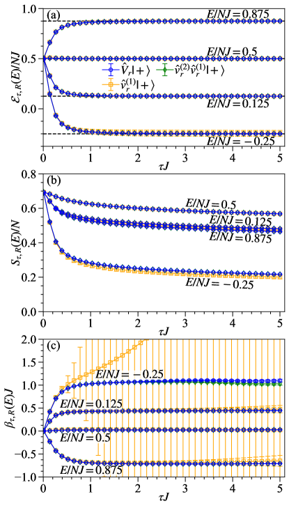
Figure 6: The same as Fig. 5 but for $N=28$. The full-diagonalization results are not shown because the huge computational resource required is not currently available.

Let us now discuss the variance due to the random samplings considered here. In the case of the random sampling for the trace evaluations using the random-phase states $\{\hat{V}_{r}|+\rangle\}_{r}$, the covariance between $A_{r}=\langle+|\hat{V}_{r}^{\dagger}\hat{A}\hat{V}_{r}|+\rangle$ and $B_{r}^{*}=\langle+|\hat{V}_{r}^{\dagger}\hat{B}^{\dagger}\hat{V}_{r}|+\rangle$ decreases as in Eq. (24). Here, $\hat{\cal H}$, $\hat{G}_{\tau}(E)$, and $\hat{\cal H}\hat{G}_{\tau}(E)$ are relevant for operators $\hat{A}$ and $\hat{B}$. Since $|\langle b|\hat{G}_{\tau}(E)|b\rangle|=O(1)$, $|\langle b|\hat{\cal H}\hat{G}_{\tau}(E)|b\rangle|=O(N)$, ${\rm Tr}[\hat{G}_{\tau}^{2}(E)]={\rm Tr}[\hat{G}_{\sqrt{2}\tau}(E)]=O(D)$, and ${\rm Tr}[\hat{\cal H}^{2}\hat{G}_{\tau}^{2}(E)]=O(DN^{2})$, the corresponding (co)variance decreases as $1/D$, i.e., exponentially in the system size $N$ (see Sec. III.2). Since the diagonal-unitary $t$-designs can simulate up to $t$-th statistical moment of the random-phase states Nakata et al. (2014), diagonal-unitary $t$-designs with $t\geqslant 2$ also possess the property of the exponentially small (co)variance as in Eq. (24), but those with $t=1$ do not, as $A_{r}^{2}$ and $A_{r}B_{r}$ involve two $\hat{V}_{r}$’s and two $\hat{V}_{r}^{\dagger}$’s. This is thus consistent with the numerical observation that the statistical errors for $\hat{v}_{r}^{(1)}|+\rangle$ are qualitatively distinct from those for $\hat{v}_{r}^{(2)}\hat{v}_{r}^{(1)}|+\rangle$ and $\hat{V}_{r}|+\rangle$. We should note that a similar discussion for the canonical TPQ state using random Clifford circuits (i.e., not for diagonal-unitary designs) is found in the recent study Coopmans et al. (2022). Considering quantum computation, it is impractical to prepare $\hat{V}_{r}|+\rangle$ because it requires an exponentially large number of single- and two-qubit gates. Therefore, as our numerical results also clearly demonstrated, $\hat{v}_{r}^{(2)}\hat{v}_{r}^{(1)}|+\rangle$ might be an appealing choice among the random-phase states as it requires only a polynomial number of single- and two-qubit gates.

VII Conclusions and discussions

We have proposed a method to calculate thermodynamic quantities of quantum many-body systems based on microcanonical TPQ states, i.e., energy-filtered random-phase states. In this formalism, a microcanonical ensemble is specified by a target energy $E$ as well as its associated energy window of width $\delta E$, and the density of states is thus expressed by a sum of Gaussians centered at the target energy $E$ with its spread corresponding to the width of the energy window $\delta E$. Since the density of states is a continuous function of $E$ in this formalism, we can derive analytical expressions of thermodynamic quantities such as the entropy and the inverse temperature. This formalism also allows us to estimate these thermodynamic quantities by evaluating the trace of the time-evolution operator and the trace of the time-evolution operator multiplied by the Hamiltonian of the system, which is thus suitable for quantum computation. By introducing the random sampling for the trace evaluations using the random-phase states, we can recognize that our formalism is a microcanonical counterpart of the canonical TPQ state, and the corresponding TPQ state is now an energy-filtered random-phase state with the target energy $E$ and the filtering time $\tau$, the latter being related to the width of the energy window via $\delta E=\sqrt{\pi}/\tau$.

We have then numerically validated the proposed method by calculating thermodynamic quantities of the one-dimensional spin-1/2 Heisenberg model with the full diagonalization method up to $N=24$ qubits and the random sampling method up to $N=28$ qubits. It is found that the proposed method is most effective for a target energy around which a large number of energy eigenstates exist and hence the statistical-mechanical treatment of thermodynamic quantities is reasonable. We have also numerically examined three different types of the random-phase states $\hat{V}_{r}|+\rangle$, $\hat{v}_{r}^{(1)}|+\rangle$, and $\hat{v}_{r}^{(2)}\hat{v}_{r}^{(1)}|+\rangle$, the latter two being prepared by the diagonal-unitary circuits, for the random sampling of the trace evaluations. We have shown that for a fixed number $R$ of samples, the random-phase states $\hat{v}_{r}^{(2)}\hat{v}_{r}^{(1)}|+\rangle$ provide the results as accurate as $\hat{V}_{r}|+\rangle$, where they can be prepared with a polynomial number $O(N^{2})$ of one- and two-qubit gates. It is worth noting that the method for the trace evaluations using the random-phase states $\hat{V}_{r}|+\rangle_{r}$, $\hat{v}_{r}^{(1)}|+\rangle_{r}$, or $\hat{v}_{r}^{(2)}\hat{v}_{r}^{(1)}|+\rangle_{r}$ is independent of the spatial dimensions of the system, and hence the same method is expected to be applicable for computing thermodynamic quantities in higher spatial dimensions.

Considering quantum computation, the number of quantum gates required is $O(N^{2})+O(MN)$ in the present setting, where $O(N^{2})$ is for preparation of the state $\hat{v}_{r}^{(2)}\hat{v}_{r}^{(1)}|+\rangle$, and $O(MN)$ is for the time-evolution operator. If a $k$-local Hamiltonian is considered, the number of quantum gates will be $O(N^{2})+O(kMN)$, which is still polynomial in $N$. The quantum circuit corresponding to $\hat{v}_{r}^{(2)}$ consists of $O(N^{2})$ all-to-all two-qubit operations. Therefore, implementing $\hat{v}_{r}^{(2)}\hat{v}_{r}^{(1)}|+\rangle$ for large systems (e.g., $N\sim 10^{2}$) on, for example, superconducting quantum computers would be challenging. Thus implementing $\hat{v}_{r}^{(1)}|+\rangle$ instead would be a good compromise for demonstrating the proposed method using a real quantum computer as it requires only $N$ Hadamard and $N$ single-qubit-rotation gates. On the other hand, the time evolution of a quantum state by a quantum many-body Hamiltonian has been demonstrated recently Arute et al. (2020), suggesting that the time-evolution part of the circuit would be feasible in near-term quantum computers.

If the number of states around a target energy is so small that only a few energy eigenstates are found in the energy window, which often occurs especially for small systems, then the statistical-mechanical treatment of thermodynamic quantities is irrelevant. Rather, in such a case, one might be interested in these individual energy eigenvalues and eigenstates separately. While there are several methods to compute a few eigenstates of the Hamiltonian, those that are related to the present formalism are the filter-diagonalization method Wall and Neuhauser (1995) in classical computation, and the quantum filter-diagonalization method Parrish and McMahon (2019) and the related Krylov-subspace method Stair et al. (2020) in quantum computation. More recently, a Gaussian-filter method for exploring ground-state properties has been proposed He et al. (2022), where the initial state is prepared so as to have a large overlap with the target ground state, instead of being prepared as a random state. The quantum subspace expansion method such as one Seki and Yunoki (2022) based on the quantum power method Seki and Yunoki (2021) might be also useful. We also note that in a similar spirit but for the canonical ensemble in classical computation, an improved version of the finite-temperature Lanczos method by explicitly calculating low-lying eigenpairs has recently been proposed Morita and Tohyama (2020) to reduce the number of samples at low temperatures (see also Ref. Aichhorn et al. (2003) for another approach to an efficient sampling at low temperatures).

In the formalism developed here, we have introduced the width of the energy window $\delta E\sim 1/\tau$ as a spread of the Gaussian $\hat{G}_{\tau}(E)$ in Eq. (5). However, this is in principle not necessary. For example, we could also employ a more conventional rectangular function centered at $E$ with its width $\delta E$, as in the histograms in Fig. 2. A rectangular cut of the energy window is appealing for its conceptual simplicity in counting the number of states within this window. A drawback of this is that the entropy is no longer a continuous function of $E$ and hence the derivative of it with respect to $E$ is not well defined. In addition, considering the numerical simulation based on the Fourier transform of $\hat{G}_{\tau}(E)$ but with a sum of rectangular functions, there appears a cardinal sine (${\rm sinc}$) function in place of the Gaussian in the integrand of Eq. (13). The appearance of the ${\rm sinc}$ function in the time domain might be less appealing than the Gaussian from a numerical point of view because ${\rm sinc}{x}=\sin{x}/{x}$ decays slowly as $1/x$ with oscillation. Therefore, using a Gaussian instead of a rectangular function much simplifies the analytical and numerical treatments of the microcanonical ensemble. Although details of the choice for the energy window should not affect thermodynamic quantities in the thermodynamic limit, it is still interesting to explore how functional forms for $\hat{G}_{\tau}(E)$, other than the Gaussian studied here, could improve the numerical efficiency of the calculations for finite systems.

Let us now briefly discuss a possible generalization of the present method to other ensembles. To this end, let us first recall the following properties of the random-phase state $|\phi_{r}\rangle$:

$$D\lim_{R\to\infty}\langle\langle|\phi_{r}\rangle\langle\phi_{r}|\rangle\rangle_{R} =\hat{I}$$ (74)

and

$$D\langle\langle\,\langle\phi_{r}|\phi_{r}\rangle\,\rangle\rangle_{R} ={\rm Tr}\left[\hat{I}\right]=D.$$ (75)

Along with the analysis in Sec. IV.3, $|\phi_{r}\rangle$ can be considered as a pure quantum state corresponding to the uniform ensemble Tolman (1980), which is represented by a density matrix of the maximally mixed state, i.e., $\hat{\rho}_{\rm uni}\equiv\hat{I}/D$. The uniform ensemble is an ensemble used when no prior knowledge of the system is available, in the sense that all the pure states appear in $\hat{\rho}_{\rm uni}$ with the equal probability $1/D$ because the lack of knowledge can be quantified by, for example, the von Neumann entropy having the maximum value $\ln D$. The density matrix $\hat{\rho}_{\tau}(E)=\hat{G}_{\tau}(E)/{\rm Tr}[\hat{G}_{\tau}(E)]$ in Eq. (53) specifies the energy $E$ of the system and the width of the energy window $\sqrt{\pi}/\tau$, and the acquirement of such knowledge is incorporated in the pure-state formalism by multiplying $[\hat{G}_{\tau}(E)]^{\frac{1}{2}}$ to the random-phase state $|\phi_{r}\rangle$, i.e., by filtering the energy.

We can push forward the above strategy to priorly specify several physical quantities, not limited to the energy, of the system by using multiple filters. Let us introduce an operator (also see Ref. Tolman (1980))

$$\hat{\cal G}_{\hat{Q},\sigma}(Q)=\exp\left[-\frac{(\hat{Q}-Q)^{2}}{2\sigma^{2}}\right],$$ (76)

where $\hat{Q}$ is a Hermitian operator in the Hilbert space of the system and $Q$ and $\sigma$ are real parameters, hence $\hat{\cal G}_{\hat{Q},\sigma}(Q)$ being Hermitian and positive definite. We can also introduce $N_{q}$ products of such operators $\hat{\cal G}_{\vec{\hat{Q}},\vec{\sigma}}(\vec{Q})\equiv\prod_{q=1}^{N_{q}}\hat{\cal G}_{\hat{Q}_{q},\sigma_{q}}(Q_{q})$ to consider a density matrix

$$\hat{\rho}_{\vec{\hat{Q}},\vec{\sigma}}(\vec{Q})\equiv\frac{\hat{\cal G}_{\vec{\hat{Q}},\vec{\sigma}}(\vec{Q})}{{\rm Tr}\left[\hat{\cal G}_{\vec{\hat{Q}},\vec{\sigma}}(\vec{Q})\right]},$$ (77)

in which the eigenvalues of $\hat{Q}_{1},\hat{Q}_{2},\cdots,\hat{Q}_{N_{q}}$ are concentrated around $Q_{1},Q_{2},\cdots,Q_{N_{q}}$ with their variances approximately $\sigma_{1}^{2},\sigma_{2}^{2},\cdots,\sigma_{N_{q}}^{2}$. Here, we assume that $[\hat{Q}_{q},\hat{Q}_{q^{\prime}}]=0$ and $[\hat{Q}_{q},\hat{\cal H}]=0$ so that $\hat{\rho}_{\vec{\hat{Q}},\vec{\sigma}}(\vec{Q})$ is Hermitian and does not evolve in time. Examples of $\hat{Q}_{q}$ include the Hamiltonian itself, as already described above with $\hat{\cal G}_{\hat{\cal H},\frac{1}{\sqrt{2}\tau}}(E)=\hat{G}_{\tau}(E)$, the magnetization operator, the particle-number operator (for fermions or bosons), and the total-spin operator, assuming that the system preserves the corresponding symmetries. The pure state associated with $\hat{\rho}_{\vec{\hat{Q}},\vec{\sigma}}(\vec{Q})$ is given by $\hat{\cal G}_{\vec{\hat{Q}},\sqrt{2}\vec{\sigma}}(\vec{Q})|\phi_{r}\rangle$, and the Fourier representation of $\hat{\cal G}_{\vec{\hat{Q}},\vec{\sigma}}(\vec{Q})$ is given by

$$\hat{\cal G}_{\vec{\hat{Q}},\vec{\sigma}}(\vec{Q})=\prod_{q=1}^{N_{q}}\left[\frac{1}{\sqrt{2\pi}\sigma_{q}}\int_{-\infty}^{\infty}{\rm d}s_{q}{\rm e}^{-\frac{s_{q}^{2}\sigma_{q}^{2}}{2}}{\rm e}^{-{\rm i}(\hat{Q}_{q}-Q_{q})s_{q}}\right],$$ (78)

where the integration variable $s_{q}$ has the dimension of $1/Q_{q}$ [also see Eq. (13)].

It is worth noting that the above generalization can be further extended to a set of noncommuting operators $[\hat{Q}_{q},\hat{Q}_{q^{\prime}}]\not{=}0$ by replacing $\hat{\cal G}_{\vec{\hat{Q}},\vec{\sigma}}(\vec{Q})$ in Eq. (77) with

$${\cal G}_{\vec{\hat{Q}},\boldsymbol{\Sigma}}(\vec{Q})=\exp\left[-\frac{1}{2}\left(\vec{\hat{Q}}-\vec{Q}\right)^{T}\boldsymbol{\Sigma}^{-1}\left(\vec{\hat{Q}}-\vec{Q}\right)\right],$$ (79)

where $\boldsymbol{\Sigma}$ is an $N_{q}\times N_{q}$ covariance matrix whose $(i,j)$ entry approximately gives the covariance between the expectations of $\hat{Q}_{i}$ and $\hat{Q}_{j}$. ${\cal G}_{\vec{\hat{Q}},\boldsymbol{\Sigma}}(\vec{Q})$ will be relevant to generalized thermodynamic ensembles with noncommuting operators studied in the context of generalized thermodynamic resource theories Yunger Halpern et al. (2016); Halpern (2018); Yunger Halpern et al. (2020); Yunger Halpern and Majidy (2022), which are recently examined experimentally with a trapped-ion system Kranzl et al. (2022). When $\boldsymbol{\Sigma}={\rm diag}(\sigma_{1}^{2},\sigma_{2}^{2},\cdots,\sigma_{N_{q}}^{2})$ and $[\hat{Q}_{q},\hat{Q}_{q^{\prime}}]=0$, ${\cal G}_{\vec{\hat{Q}},\boldsymbol{\Sigma}}(\vec{Q})$ is reduced to $\hat{\cal G}_{\vec{\hat{Q}},\vec{\sigma}}(\vec{Q})$. We expect that it is useful to consider a variety of ensembles along these lines when we can priorly specify several physical quantities of the system associated with Hermitian operators $\hat{Q}_{1},\hat{Q}_{2},\cdots,\hat{Q}_{N_{q}}$.

Finally, we note that our formalism developed here is related to the previous work in Ref. Lu et al. (2021) (also see related works in Refs. Yang et al. (2022); Schuckert et al. (2022)). Aside from technical details, the main conceptual differences can be summarized as follows: (i) we derive the analytical expression for the inverse temperature that is not a parameter but is evaluated, covering both positive- and negative-temperature sides, and (ii) our formalism reveals a connection to a TPQ-state formalism of the microcanonical ensemble via the energy-filtered random-phase states that are closely related to the states introduced in a different context to extract eigenvalues and eigenstates of $\hat{H}$ at any desired energy range, known as the filter-diagonalization method Wall and Neuhauser (1995).

Appendix A Cumulative number of states

In this Appendix, we discuss the cumulative number of states. The cumulative number of states $W_{\tau}(E)$ below energy $E$ is given by

$$W_{\tau}(E)=\int_{-\infty}^{E}{\rm d}E^{\prime}g_{\tau}(E^{\prime})=\frac{1}{2}\sum_{n=0}^{D-1}{\rm erfc}[(E_{n}-E)\tau],$$ (80)

where ${\rm erfc}(x)=\frac{2}{\sqrt{\pi}}\int_{x}^{\infty}{\rm d}y\ {\rm e}^{-y^{2}}$ is the complementary error function, satisfying that ${\rm erfc}(-\infty)=2$ and ${\rm erfc}(\infty)=0$. Hence, the total number of states is given by $W_{\tau}(\infty)=D$. Note also that $\frac{1}{2}{\rm erfc}(-x\tau)$ is reduced to the step function $\theta(x)$, i.e., $\theta(x)=1$ for $x>0$ and $\theta(x)=0$ for $x<0$, in the limit of $\tau\to\infty$. In other words, for finite $\tau$, the cumulative number of states $W_{\tau}(E)$ is a continuous function of $E$ and in general not integer because $W_{\tau}(E)$ is not a sum of step functions. The number of states within the range of $[E-\delta E/2,E+\delta E/2)$ for small $\delta E$ is given by

$$W_{\tau}\left(E+\frac{\delta E}{2}\right)-W_{\tau}\left(E-\frac{\delta E}{2}\right) =\int_{E-\frac{\delta E}{2}}^{E+\frac{\delta E}{2}}{\rm d}E^{\prime}g_{\tau}(E^{\prime})$$

$$\sim g_{\tau}(E)\delta E,$$ (81)

where the integrand $g_{\tau}(E^{\prime})$ is approximated by its representative value at the mid point, $g_{\tau}(E)$. The argument in the logarithm of Eq. (2) is exactly the quantity in Eq. (81) with $\delta E$ given in Eq. (11).

Appendix B Equivalence between Eq. (32) and Eq. (49)

In this Appendix, we prove the equivalence between Eq. (32) and Eq. (49). From Eq. (42), the squared norm of the energy-filtered random-phase state $|\psi_{\tau,r}(E)\rangle$ can be expressed as

$$\langle\psi_{\tau,r}(E)|\psi_{\tau,r}(E)\rangle$$

$$= \frac{1}{2\pi\tau^{2}}\int_{-\infty}^{\infty}{\rm d}s\int_{-\infty}^{\infty}{\rm d}t\ {\rm e}^{-\frac{s^{2}+t^{2}}{2\tau^{2}}}{\rm e}^{{\rm i}E(t-s)}\langle\phi_{r}|\hat{U}(t-s)|\phi_{r}\rangle$$

$$= \frac{1}{4\pi\tau^{2}}\int_{-\infty}^{\infty}{\rm d}t_{+}\int_{-\infty}^{\infty}{\rm d}t_{-}\ {\rm e}^{-\frac{t_{+}^{2}+t_{-}^{2}}{4\tau^{2}}}{\rm e}^{{\rm i}Et_{-}}\langle\phi_{r}|\hat{U}(t_{-})|\phi_{r}\rangle$$

$$= \frac{1}{2\sqrt{\pi}\tau}\int_{-\infty}^{\infty}{\rm d}t_{-}\ {\rm e}^{-\frac{t_{-}^{2}}{4\tau^{2}}}{\rm e}^{{\rm i}Et_{-}}\langle\phi_{r}|\hat{U}(t_{-})|\phi_{r}\rangle.$$ (82)

where the variables are changed from $s$ and $t$ to $t_{+}\equiv t+s$ and $t_{-}\equiv t-s$ in the second equality, and the integral over $t_{+}$ is performed in the third equality. Note that by the change of variables in the second equality, the volume element is transformed as ${\rm d}s{\rm d}t=\left|\frac{\partial(s,t)}{\partial(t_{+},t_{-})}\right|{\rm d}t_{+}{\rm d}t_{-}$ with the Jacobian determinant $\frac{\partial(s,t)}{\partial(t_{+},t_{-})}=\frac{1}{2}$. By substituting $K_{r}(t_{-})=\langle\phi_{r}|\hat{U}(t_{-})|\phi_{r}\rangle$ into Eq. (82), we obtain Eq. (32), and hence the equivalence between Eq. (32) and Eq. (49) is proved. The equivalence between Eq. (33) and Eq. (50) can also be proved similarly.

Appendix C Translation to canonical ensemble

In this Appendix, we discuss how the present formalism of the microcanonical ensemble can be translated into the canonical ensemble. Although thermodynamic quantities calculated with the microcanonical ensemble should be identical to those with the canonical ensemble in the thermodynamic limit, this does not hold generally for finite systems. On one hand, there may be a case where one wishes to specify the inverse temperature $\beta$ rather than the target energy $E$ as a parameter, and hence wishes to use the canonical ensemble rather than the microcanonical ensemble. On the other hand, it is well known that the partition function $Z_{\rm can}(\beta)$ of the canonical ensemble can be formally written as

$$Z_{\rm can}(\beta)\equiv{\rm Tr}\left[{\rm e}^{-\beta\hat{\cal H}}\right]=\sum_{n=0}^{D-1}\int_{-\infty}^{\infty}{\rm d}E{\rm e}^{-\beta E}\delta(E_{n}-E).$$ (83)

From the partition function $Z_{\rm can}(\beta)$, the canonical energy and the canonical entropy can be calculated as $E_{\rm can}(\beta)=-\partial_{\beta}\ln Z_{\rm can}(\beta)$ and $S_{\rm can}(\beta)=\beta E_{\rm can}(\beta)+\ln Z_{\rm can}(\beta)$, respectively.

Now, in order to be compatible with the formalism of the microcanonical ensemble considered here, let us define a $\tau$-dependent partition function

$$Z_{{\rm can},\tau}(\beta)\equiv\int_{-\infty}^{\infty}{\rm d}E{\rm e}^{-\beta E}g_{\tau}(E).$$ (84)

Because $g_{\tau}(E)$ is a sum of Gaussians, the integral can be performed analytically and it results in

$$Z_{{\rm can},\tau}(\beta)=\sum_{n=0}^{D-1}{\rm e}^{-\beta E_{n}+\frac{\beta^{2}}{4\tau^{2}}}={\rm e}^{\frac{\beta^{2}}{4\tau^{2}}}Z_{\rm can}(\beta).$$ (85)

Accordingly, we define a $\tau$-dependent canonical energy and a $\tau$-dependent canonical entropy as

$$E_{{\rm can},\tau}(\beta) \equiv-\frac{\partial}{\partial\beta}\ln Z_{{\rm can},\tau}(\beta)=E_{\rm can}(\beta)-\frac{\beta}{2\tau^{2}}$$ (86)

and

$$S_{{\rm can},\tau}(\beta) \equiv\beta E_{{\rm can},\tau}(\beta)+\ln Z_{{\rm can},\tau}(\beta)=S_{\rm can}(\beta)-\frac{\beta^{2}}{4\tau^{2}},$$ (87)

respectively. Note that $\beta$ here is not calculated as in the microcanonical ensemble but it is simply a parameter. Figure 7 shows $E_{{\rm can},\tau}(\beta)$ and $S_{{\rm can},\tau}(\beta)$ for the one-dimensional spin-1/2 Heisenberg model $\hat{\mathcal{H}}$ in Eq. (57) with $N=24$ qubits calculated by the full diagonalization method. As expected from Eqs. (86) and (87), the results converge to those of the canonical ensemble, $E_{{\rm can}}(\beta)$ and $S_{{\rm can}}(\beta)$, with increasing $\tau$.

Finally, when the random sampling method for the trace evaluation is employed, the $\tau$-dependent partition function $Z_{{\rm can},\tau}(\beta)$ should be calculated by replacing $g_{\tau}(E)$ with $g_{\tau,R}(E)$ in Eq. (84) [see Eqs. (32) and (36)]. Accordingly, the $\tau$-dependent partition function $Z_{{\rm can},\tau}(\beta)$ as well as the $\tau$-dependent canonical energy $E_{{\rm can},\tau}(\beta)$ and the $\tau$-dependent canonical entropy $S_{{\rm can},\tau}(\beta)$ acquires statistical errors.

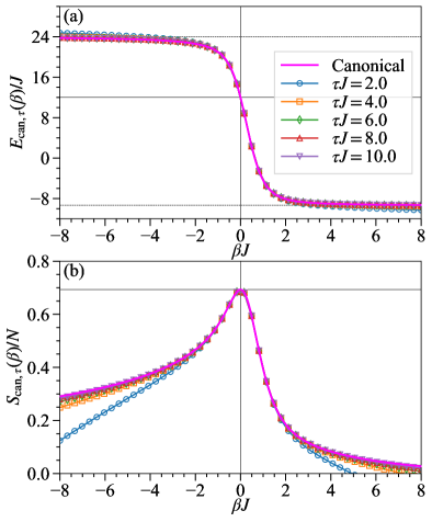
Figure 7: (a) The $\tau$-dependent canonical energy $E_{{\rm can},\tau}(\beta)$ and (b) the $\tau$-dependent canonical entropy $S_{{\rm can},\tau}(\beta)$ as a function of the inverse temperature $\beta$ for several $\tau$ values for $N=24$. The solid magenta lines in (a) and (b) indicate the canonical energy $E_{{\rm can}}(\beta)$ and the canonical entropy $S_{{\rm can}}(\beta)$, respectively. In (a), the dashed horizontal lines indicate $E_{0}$ and $E_{D-1}$, and the solid horizontal line indicates $JN_{\rm bond}/2=12J$, corresponding to the energy at $\beta=0$. In (b), the horizontal line indicates $\ln 2$, corresponding to the entropy per qubit at $\beta=0$.

Appendix D Average of the random-phase-product states

In this Appendix, we show that the random-phase-product states of the form $v_{r}^{(1)}|+\rangle$ satisfy Eq. (27). The ideal random average for the states $v_{r}^{(1)}|+\rangle$ parametrized as in Eq. (59), where $N_{v}=N$, is given by $\mathbb{E}_{N}[A_{r}]=\frac{1}{(2\pi)^{N}}\int_{0}^{2\pi}{\rm d}\theta_{0,r}\int_{0}^{2\pi}{\rm d}\theta_{1,r}\cdots\int_{0}^{2\pi}{\rm d}\theta_{N-1,r}A_{r}.$ We can then easily show that

$$\mathbb{E}_{N}\left[\prod_{k=0}^{N-1}{\rm e}^{{\rm i}\theta_{k,r}\left\{(-1)^{b_{k}}-(-1)^{b_{k}^{\prime}}\right\}/2}\right]=\prod_{k=0}^{N-1}\delta_{b_{k}b_{k}^{\prime}}=\delta_{bb^{\prime}}$$ (88)

and thus $\hat{v}_{r}^{(1)}|+\rangle$ satisfy Eq. (27). Here, $b_{k}$ and $b_{k}^{\prime}$ are binary ($0$ or $1$) variables at the $k$th qubit, and $b$ and $b^{\prime}$ are the corresponding bit strings of length $N$, $\{b_{k}\}_{k=0}^{N-1}$ and $\{b^{\prime}_{k}\}_{k=0}^{N-1}$, respectively.

Instead of the continuous random variables, we can consider $\{\theta_{k,r}\}_{k=0}^{N-1}$ as a set of discrete random variables drawn uniformly from $\{0,\pi\}^{N}$, $\{0,\frac{2\pi}{3},\frac{4\pi}{3}\}^{N}$, or in general $\{0,\frac{2\pi}{l},\frac{2\pi\times 2}{l},\cdots\frac{2\pi(l-1)}{l}\}^{N}$ with $l>0$ integer. In this case, the ideal random average is given by $\mathbb{E}_{N}[A_{r}]=\frac{1}{l^{N}}\sum_{\theta_{0,r}=0}^{2\pi(l-1)/l}\sum_{\theta_{1,r}=0}^{2\pi(l-1)/l}\cdots\sum_{\theta_{N-1,r}=0}^{2\pi(l-1)/l}A_{r}$, and one can also readily confirm that Eq. (88) and hence Eq. (27) are still satisfied. A finite set of random diagonal unitaries $\{\hat{v}_{r}^{(1)}\}$ with discrete random variables corresponds to the diagonal-unitary 1-design.

Appendix E Additional numerical results

E.1 Numerical results for smaller systems

Figure 8 shows exactly the same results as in Fig. 2 but for $N=14$, 16, and 18. The values of $\tau$ used for evaluating ${\rm Tr}\left[\hat{G}_{\tau}(E)\right]=g_{\tau}(E)\delta E$ are $\tau J=$2.81, 2.46, 2.19 for $N_{\rm bin}=32$ and $N=14,16,18$, $\tau J=$5.72, 5.01, 4.46 for $N_{\rm bin}=64$ and $N=14,16,18$, and $\tau J=$11.5, 10.1, 8.99 for $N_{\rm bin}=128$ and $N=14,16,18$, respectively. As discussed in Sec. VI.1, $g_{\tau}(E)\delta E$ becomes more snaky for the smaller $N$ and the larger $N_{\rm bin}$.

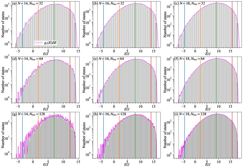
Figure 8: The same as Fig. 2 but for $N=14$, 16, and 18. The thick vertical lines at $E/NJ=-0.25,0.125,0.5,$ and $0.875$ (indicated by blue, orange, green, and red, respectively) denote the target energies used in the results shown in Figs. 9 and 10.

Figure 9 shows exactly the same results as in Fig. 3 but for $N=14$, 16, and 18. As compared to ${\cal E}_{\tau}(E)$ and $S_{\tau}(E)$, the inverse temperature $\beta_{\tau}(E)$ depends rather wildly on the filtering time $\tau$. In particular, the inverse temperature for $E/NJ=-0.25$ becomes negative for $\tau J\gtrsim 4$. However, as shown in Figs. 3 and 6 (also see Fig. 12), such a wild dependence on $\tau$ is moderated for the larger systems.

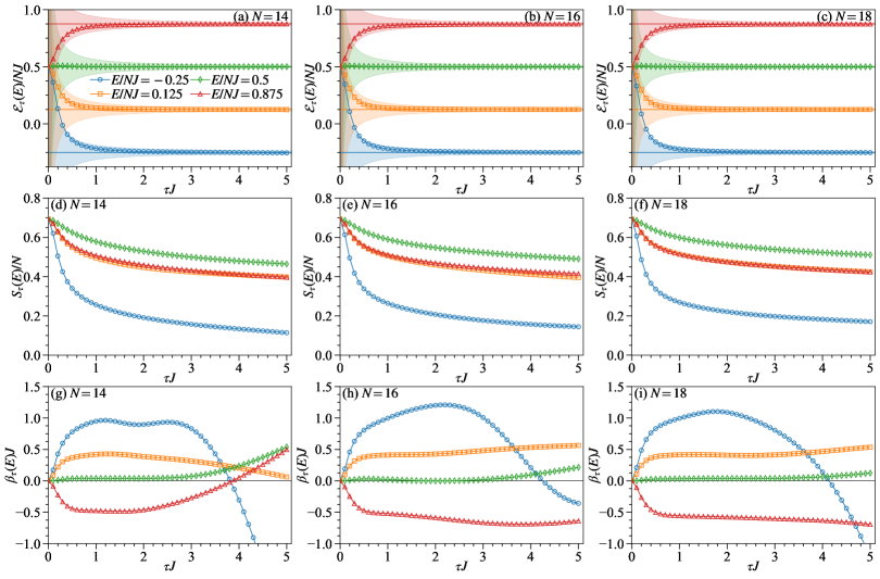
Figure 9: The same as Fig. 3 but for $N=14$, 16, and 18.

Figure 10 shows exactly the same results as in Fig. 4 but for $N=14$, 16, and 18. As expected, the energy fluctuation $\sigma_{\tau}(E)$ for large $\tau$ behaves as $\sigma_{\tau}(E)\sim 1/\sqrt{2}\tau$, independently of the system size $N$. It is also found that the dependence of $\sigma_{\tau}(E)$ on the target energy $E$ becomes less significant and matches better with $1/\sqrt{2}\tau$ for the larger systems [see insets in Figs. 10(d)–10(f)].

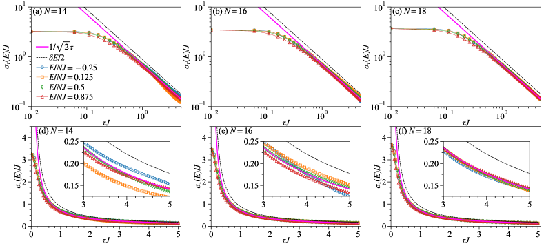
Figure 10: The same as Fig. 4 but for $N=14$, 16, and 18.

E.2 Detailed results on random sampling for trace evaluation

Here we provide detailed results on the random sampling method for the trace evaluations. Figure 11 shows the same results as in Fig. 5 for $N=24$ but plotted separately for the different target energies $E/NJ=0.875$, $0.5$, $0.125$, and $-0.25$. It is clearly observed that the statistical errors with the the random-phase states $\hat{v}_{r}^{(1)}|+\rangle$ behave qualitatively differently from those with the other random-phase states $\hat{v}_{r}^{(2)}\hat{v}_{r}^{(1)}|+\rangle$ and $\hat{V}_{r}|+\rangle$. The same trend is found for the larger system of $N=28$, as shown in Fig. 12.

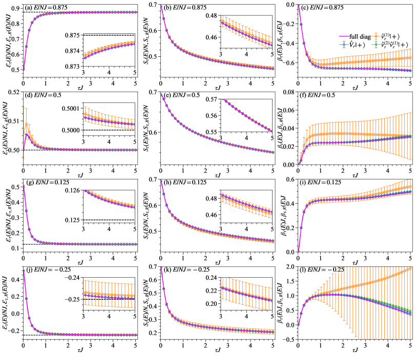
Figure 11: The same results as in Fig. 5 but plotted separately for the different target energies $E/NJ=0.875$, $0.5$, $0.125$, and $-0.25$. (a,d,g,j) The energy expectation value ${\cal E}_{\tau,R}(E)$, (b,e,h,k) the entropy $S_{\tau,R}(E)$, and (c,f,i,l) the inverse temperature $\beta_{\tau,R}(E)$ as a function of the filtering time $\tau$ for $N=24$. The black dashed horizontal lines in (a), (d), (g), and (j) indicate the target energies. The insets show the magnifications for $3\leqslant\tau J\leqslant 5$. Notice that the different panels employ the different scales in the $y$ axis.

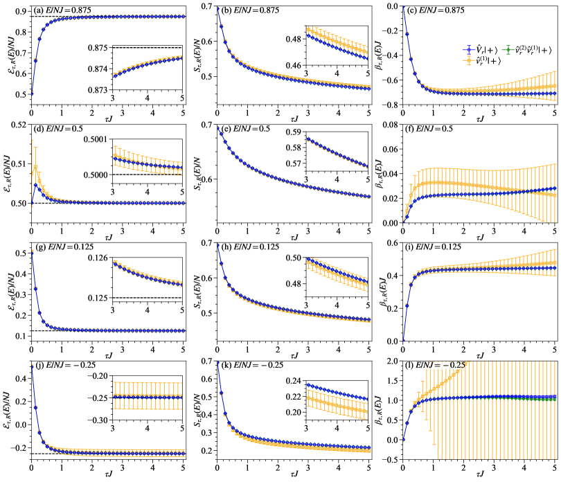
Figure 12: The same as in Fig. 11 but for $N=28$. The full-diagonalization results are not shown because the huge computational resource required is not currently available.

References

- Fano (1957) U. Fano, “Description of States in Quantum Mechanics by Density Matrix and Operator Techniques,” Rev. Mod. Phys. 29, 74–93 (1957).
- Suzuki (1985) Masuo Suzuki, “Thermo field dynamics in equilibrium and non-equilibrium interacting quantum systems,” Journal of the Physical Society of Japan 54, 4483–4485 (1985).
- Feiguin and White (2005) Adrian E. Feiguin and Steven R. White, “Finite-temperature density matrix renormalization using an enlarged Hilbert space,” Phys. Rev. B 72, 220401 (2005).
- Nomura et al. (2021) Yusuke Nomura, Nobuyuki Yoshioka, and Franco Nori, “Purifying Deep Boltzmann Machines for Thermal Quantum States,” Phys. Rev. Lett. 127, 060601 (2021).
- Li and Haldane (2008) Hui Li and F. D. M. Haldane, “Entanglement Spectrum as a Generalization of Entanglement Entropy: Identification of Topological Order in Non-Abelian Fractional Quantum Hall Effect States,” Phys. Rev. Lett. 101, 010504 (2008).
- Poilblanc (2010) Didier Poilblanc, “Entanglement Spectra of Quantum Heisenberg Ladders,” Phys. Rev. Lett. 105, 077202 (2010).
- Qi et al. (2012) Xiao-Liang Qi, Hosho Katsura, and Andreas W. W. Ludwig, “General Relationship between the Entanglement Spectrum and the Edge State Spectrum of Topological Quantum States,” Phys. Rev. Lett. 108, 196402 (2012).
- Dalmonte et al. (2018) M. Dalmonte, B. Vermersch, and P. Zoller, “Quantum simulation and spectroscopy of entanglement Hamiltonians,” Nature Physics 14, 827–831 (2018).
- Giudici et al. (2018) G. Giudici, T. Mendes-Santos, P. Calabrese, and M. Dalmonte, “Entanglement Hamiltonians of lattice models via the Bisognano-Wichmann theorem,” Phys. Rev. B 98, 134403 (2018).
- Mendes-Santos et al. (2020) T. Mendes-Santos, G. Giudici, R. Fazio, and M. Dalmonte, “Measuring von Neumann entanglement entropies without wave functions,” New Journal of Physics 22, 013044 (2020).
- Seki and Yunoki (2020a) Kazuhiro Seki and Seiji Yunoki, “Emergence of a thermal equilibrium in a subsystem of a pure ground state by quantum entanglement,” Phys. Rev. Research 2, 043087 (2020a).
- Tolman (1980) Richard C. Tolman, The Principles of Statistical Mechanics (Dover, New York, 1980) Chap. IX.
- Drabold and Sankey (1993) David A. Drabold and Otto F. Sankey, “Maximum entropy approach for linear scaling in the electronic structure problem,” Phys. Rev. Lett. 70, 3631–3634 (1993).
- Iitaka and Ebisuzaki (2004) Toshiaki Iitaka and Toshikazu Ebisuzaki, “Random phase vector for calculating the trace of a large matrix,” Phys. Rev. E 69, 057701 (2004).
- Weiße et al. (2006) Alexander Weiße, Gerhard Wellein, Andreas Alvermann, and Holger Fehske, “The kernel polynomial method,” Rev. Mod. Phys. 78, 275–306 (2006).
- Jin et al. (2021) Fengpin Jin, Dennis Willsch, Madita Willsch, Hannes Lagemann, Kristel Michielsen, and Hans De Raedt, “Random State Technology,” Journal of the Physical Society of Japan 90, 012001 (2021).
- Jaklič and Prelovšek (1994) J. Jaklič and P. Prelovšek, “Lanczos method for the calculation of finite-temperature quantities in correlated systems,” Phys. Rev. B 49, 5065–5068 (1994).
- Prelovšek and Bonča (2013) P. Prelovšek and J. Bonča, “Ground State and Finite Temperature Lanczos Methods,” in Strongly Correlated Systems: Numerical Methods, edited by Adolfo Avella and Ferdinando Mancini (Springer Berlin Heidelberg, Berlin, Heidelberg, 2013) pp. 1–30.
- Sugiura and Shimizu (2013) Sho Sugiura and Akira Shimizu, “Canonical Thermal Pure Quantum State,” Phys. Rev. Lett. 111, 010401 (2013).
- Long et al. (2003) M. W. Long, P. Prelovšek, S. El Shawish, J. Karadamoglou, and X. Zotos, “Finite-temperature dynamical correlations using the microcanonical ensemble and the Lanczos algorithm,” Phys. Rev. B 68, 235106 (2003).
- Okamoto et al. (2018) Satoshi Okamoto, Gonzalo Alvarez, Elbio Dagotto, and Takami Tohyama, “Accuracy of the microcanonical Lanczos method to compute real-frequency dynamical spectral functions of quantum models at finite temperatures,” Phys. Rev. E 97, 043308 (2018).
- Sugiura and Shimizu (2012) Sho Sugiura and Akira Shimizu, “Thermal Pure Quantum States at Finite Temperature,” Phys. Rev. Lett. 108, 240401 (2012).
- Seki and Yunoki (2020b) Kazuhiro Seki and Seiji Yunoki, “Thermodynamic properties of an ring-exchange model on the triangular lattice,” Phys. Rev. B 101, 235115 (2020b).
- Suzuki (1990) Masuo Suzuki, “Fractal decomposition of exponential operators with applications to many-body theories and Monte Carlo simulations,” Physics Letters A 146, 319 – 323 (1990).
- Wall and Neuhauser (1995) Michael R. Wall and Daniel Neuhauser, “Extraction, through filter-diagonalization, of general quantum eigenvalues or classical normal mode frequencies from a small number of residues or a short-time segment of a signal. I. Theory and application to a quantum-dynamics model,” The Journal of Chemical Physics 102, 8011–8022 (1995).
- Challa and Hetherington (1988) Murty S. S. Challa and J. H. Hetherington, “Gaussian ensemble: An alternate Monte Carlo scheme,” Phys. Rev. A 38, 6324–6337 (1988).
- Yoneta and Shimizu (2019) Yasushi Yoneta and Akira Shimizu, “Squeezed ensemble for systems with first-order phase transitions,” Phys. Rev. B 99, 144105 (2019).
- Nakata et al. (2014) Yoshifumi Nakata, Masato Koashi, and Mio Murao, “Generating a state -design by diagonal quantum circuits,” New Journal of Physics 16, 053043 (2014).
- Nakata et al. (2012) Yoshifumi Nakata, Peter S. Turner, and Mio Murao, “Phase-random states: Ensembles of states with fixed amplitudes and uniformly distributed phases in a fixed basis,” Phys. Rev. A 86, 012301 (2012).
- Iwaki and Hotta (2022) Atsushi Iwaki and Chisa Hotta, “Purity of thermal mixed quantum states,” Phys. Rev. B 106, 094409 (2022).
- Dankert et al. (2009) Christoph Dankert, Richard Cleve, Joseph Emerson, and Etera Livine, “Exact and approximate unitary 2-designs and their application to fidelity estimation,” Phys. Rev. A 80, 012304 (2009).
- Iitaka (2020) Toshiaki Iitaka, “Random Phase Product State for Canonical Ensemble,” (2020), arXiv:2006.14459 [cond-mat.str-el] .
- Nakata et al. (2017a) Yoshifumi Nakata, Christoph Hirche, Ciara Morgan, and Andreas Winter, “Unitary 2-designs from random - and -diagonal unitaries,” Journal of Mathematical Physics 58, 052203 (2017a).
- Nakata et al. (2017b) Yoshifumi Nakata, Christoph Hirche, Masato Koashi, and Andreas Winter, “Efficient Quantum Pseudorandomness with Nearly Time-Independent Hamiltonian Dynamics,” Phys. Rev. X 7, 021006 (2017b).
- Trotter (1959) H. F. Trotter, “On the product of semi-groups of operators,” Proc. Am. Math. Soc. 10, 545 (1959).
- Suzuki (1976) Masuo Suzuki, “Generalized Trotter’s formula and systematic approximants of exponential operators and inner derivations with applications to many-body problems,” Comm. Math. Phys. 51, 183–190 (1976).
- Seki et al. (2020) Kazuhiro Seki, Tomonori Shirakawa, and Seiji Yunoki, “Symmetry-adapted variational quantum eigensolver,” Phys. Rev. A 101, 052340 (2020).
- Iwaki et al. (2021) Atsushi Iwaki, Akira Shimizu, and Chisa Hotta, “Thermal pure quantum matrix product states recovering a volume law entanglement,” Phys. Rev. Research 3, L022015 (2021).
- Goto et al. (2021) Shimpei Goto, Ryui Kaneko, and Ippei Danshita, “Matrix product state approach for a quantum system at finite temperatures using random phases and Trotter gates,” Phys. Rev. B 104, 045133 (2021).
- Coopmans et al. (2022) Luuk Coopmans, Yuta Kikuchi, and Marcello Benedetti, “Predicting Gibbs State Expectation Values with Pure Thermal Shadows,” (2022), arXiv:2206.05302 [quant-ph] .
- Arute et al. (2020) Frank Arute, Kunal Arya, Ryan Babbush, Dave Bacon, Joseph C. Bardin, Rami Barends, Andreas Bengtsson, Sergio Boixo, Michael Broughton, Bob B. Buckley, David A. Buell, Brian Burkett, Nicholas Bushnell, Yu Chen, Zijun Chen, Yu-An Chen, Ben Chiaro, Roberto Collins, Stephen J. Cotton, William Courtney, Sean Demura, Alan Derk, Andrew Dunsworth, Daniel Eppens, Thomas Eckl, Catherine Erickson, Edward Farhi, Austin Fowler, Brooks Foxen, Craig Gidney, Marissa Giustina, Rob Graff, Jonathan A. Gross, Steve Habegger, Matthew P. Harrigan, Alan Ho, Sabrina Hong, Trent Huang, William Huggins, Lev B. Ioffe, Sergei V. Isakov, Evan Jeffrey, Zhang Jiang, Cody Jones, Dvir Kafri, Kostyantyn Kechedzhi, Julian Kelly, Seon Kim, Paul V. Klimov, Alexander N. Korotkov, Fedor Kostritsa, David Landhuis, Pavel Laptev, Mike Lindmark, Erik Lucero, Michael Marthaler, Orion Martin, John M. Martinis, Anika Marusczyk, Sam McArdle, Jarrod R. McClean, Trevor McCourt, Matt McEwen, Anthony Megrant, Carlos Mejuto-Zaera, Xiao Mi, Masoud Mohseni, Wojciech Mruczkiewicz, Josh Mutus, Ofer Naaman, Matthew Neeley, Charles Neill, Hartmut Neven, Michael Newman, Murphy Yuezhen Niu, Thomas E. O’Brien, Eric Ostby, Bálint Pató, Andre Petukhov, Harald Putterman, Chris Quintana, Jan-Michael Reiner, Pedram Roushan, Nicholas C. Rubin, Daniel Sank, Kevin J. Satzinger, Vadim Smelyanskiy, Doug Strain, Kevin J. Sung, Peter Schmitteckert, Marco Szalay, Norm M. Tubman, Amit Vainsencher, Theodore White, Nicolas Vogt, Z. Jamie Yao, Ping Yeh, Adam Zalcman, and Sebastian Zanker, “Observation of separated dynamics of charge and spin in the Fermi-Hubbard model,” (2020), arXiv:2010.07965 [quant-ph] .
- Parrish and McMahon (2019) Robert M. Parrish and Peter L. McMahon, “Quantum Filter Diagonalization: Quantum Eigendecomposition without Full Quantum Phase Estimation,” (2019), arXiv:1909.08925 [quant-ph] .
- Stair et al. (2020) Nicholas H. Stair, Renke Huang, and Francesco A. Evangelista, “A Multireference Quantum Krylov Algorithm for Strongly Correlated Electrons,” Journal of Chemical Theory and Computation 16, 2236–2245 (2020).
- He et al. (2022) Min-Quan He, Dan-Bo Zhang, and Z. D. Wang, “Quantum Gaussian filter for exploring ground-state properties,” Phys. Rev. A 106, 032420 (2022).
- Seki and Yunoki (2022) Kazuhiro Seki and Seiji Yunoki, “Spatial, spin, and charge symmetry projections for a Fermi-Hubbard model on a quantum computer,” Phys. Rev. A 105, 032419 (2022).
- Seki and Yunoki (2021) Kazuhiro Seki and Seiji Yunoki, “Quantum Power Method by a Superposition of Time-Evolved States,” PRX Quantum 2, 010333 (2021).
- Morita and Tohyama (2020) Katsuhiro Morita and Takami Tohyama, “Finite-temperature properties of the Kitaev-Heisenberg models on kagome and triangular lattices studied by improved finite-temperature Lanczos methods,” Phys. Rev. Research 2, 013205 (2020).
- Aichhorn et al. (2003) Markus Aichhorn, Maria Daghofer, Hans Gerd Evertz, and Wolfgang von der Linden, “Low-temperature Lanczos method for strongly correlated systems,” Phys. Rev. B 67, 161103 (2003).
- Yunger Halpern et al. (2016) Nicole Yunger Halpern, Philippe Faist, Jonathan Oppenheim, and Andreas Winter, “Microcanonical and resource-theoretic derivations of the thermal state of a quantum system with noncommuting charges,” Nature Communications 7, 12051 (2016).
- Halpern (2018) Nicole Yunger Halpern, “Beyond heat baths II: framework for generalized thermodynamic resource theories,” Journal of Physics A: Mathematical and Theoretical 51, 094001 (2018).
- Yunger Halpern et al. (2020) Nicole Yunger Halpern, Michael E. Beverland, and Amir Kalev, “Noncommuting conserved charges in quantum many-body thermalization,” Phys. Rev. E 101, 042117 (2020).
- Yunger Halpern and Majidy (2022) Nicole Yunger Halpern and Shayan Majidy, “How to build hamiltonians that transport noncommuting charges in quantum thermodynamics,” npj Quantum Information 8, 10 (2022).
- Kranzl et al. (2022) Florian Kranzl, Aleksander Lasek, Manoj K. Joshi, Amir Kalev, Rainer Blatt, Christian F. Roos, and Nicole Yunger Halpern, “Experimental observation of thermalisation with noncommuting charges,” (2022), arXiv:2202.04652 [quant-ph] .
- Lu et al. (2021) Sirui Lu, Mari Carmen Bañuls, and J. Ignacio Cirac, “Algorithms for Quantum Simulation at Finite Energies,” PRX Quantum 2, 020321 (2021).
- Yang et al. (2022) Yilun Yang, J. Ignacio Cirac, and Mari Carmen Bañuls, “Classical algorithms for many-body quantum systems at finite energies,” Phys. Rev. B 106, 024307 (2022).
- Schuckert et al. (2022) Alexander Schuckert, Annabelle Bohrdt, Eleanor Crane, and Michael Knap, “Probing finite-temperature observables in quantum simulators with short-time dynamics,” (2022), arXiv:2206.01756 [quant-ph] .