Hyperbolic fringe signal for twin impurity quasiparticle interference

Abstract

We study the quasiparticle interference (QPI) pattern emanating from a pair of adjacent impurities on the surface of a gapped superconductor (SC). We find that hyperbolic fringes (HF) in the QPI signal can appear due to the loop contribution of the two-impurity scattering, where the location of the two impurities are the hyperbolic focus points. For a single pocket Fermiology, an HF pattern signals chiral SC order for non-magnetic impurities and requires magnetic impurities for non-chiral SC. For a multi-pocket scenario, a sign-changing order parameter such as $s_{\pm}$-wave likewise yields an HF signature. We discuss twin impurity QPI as a new tool to complement the analysis of superconducting order from local spectroscopy.

Introduction.— Quasiparticle interference (QPI) around impurities, which can be probed through a scanning tunneling microscopy (STM) measurement, has acquired a pivotal role in exploring the properties of unconventional electronic states of matter including high-$T_{c}$ superconductors (SCs) Byers et al. (1993); Hoffman et al. (2002); Wang and Lee (2003); Hanaguri et al. (2010); Sykora and Coleman (2011); Zheng and Hasan (2018); Akbari et al. (2010); Bena (2016) and topological insulators (TIs) Roushan et al. (2009); Lee et al. (2009). For SC, the local density of states (LDOS) modulation patterns not only reflect principal features of electronic dispersion and pairing symmetries Byers et al. (1993); Balatsky et al. (2006); Yu (1965); Mashkoori et al. (2017), but are also sensitive to sign changes in the SC order parameter Wang and Lee (2003); Hanaguri et al. (2010); Sykora and Coleman (2011) as well as to time-reversal symmetry Lee et al. (2009); Queiroz and Stern (2018). In addition to QPI patterns arising from a single impurity, the LDOS distribution and possible bound states due to the presence of multiple impurities have been studied in a variety of systems Flatté and Reynolds (2000); Morr and Stavropoulos (2003); Choi (2004); Zhu et al. (2003); Cano and Paul (2009); Ortuzar et al. (2022).

The QPI pattern’s phase sensitivity renders it preeminently suited to resolve intricate properties of an unconventional SC state of matter. At present, the evidence on the nature of unconventional pairing symmetry of several material classes is still incomplete. This includes candidates for chiral SC order such as strontium ruthenate Pustogow et al. (2019), Na-doped cobaltates Kiesel et al. (2013) or, more lately, Sn/Si heterostructures Wolf et al. (2022) and kagome metals Neupert et al. (2022). Likewise, additional ways to track the sign-changing nature of extended s-wave order, as suspected for many iron pnictide families, are highly sought after Stewart (2011).

In this Letter, we propose a hyperbolic fringe (HF) signal fingerprint found in the QPI pattern of two adjacent impurities deposited on a gapped SC, which we coin twin QPI. We find that through the HF signal, the twin QPI pattern allows to retrieve information beyond the single impurity case, and thus to draw conclusions on the either chiral or multi-pocket sign changing nature of the SC order parameter.

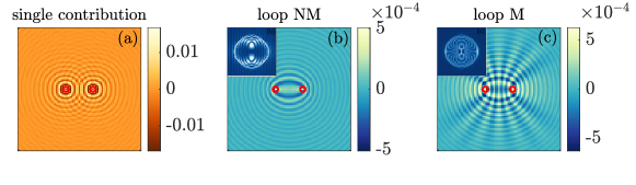
Figure 1: Twin impurity QPI for a single-pocket $s$-wave SC ($\mu=-3$, $\Delta=0.1$, $\omega=1.1\Delta$, $d=18$) in real space. Note that the shown LDOS is measured in units of $(ta^{2})^{-1}$ and thus dimensionless for our choice of $a=1$ and $t=1$. (a) Single impurity contribution to the QPI pattern. (b) Loop contribution to QPI for non-magnetic (NM) twin impurities. (c) Loop contribution to QPI for magnetic (M) twin impurities. The insets show the Fourier transformation of the patterns. A hyperbolic fringe (HF) pattern emerges on top of the elliptical fringe background.

Minimal model.— In order to complement the numerical analysis with an analytically tractable limit to showcase the mathematical structure of the HF pattern, we initially constrain ourselves to the simplest Bardeen-Cooper-Schrieffer (BCS) Hamiltonian for a single electronic band with nearest neighbor hybridization on a square lattice $\varepsilon_{\mathbf{k}}=-2t(\cos k_{x}+\cos k_{y})-\mu$:

$$H=\sum_{\mathbf{k}s}\varepsilon_{\mathbf{k}}c_{\mathbf{k}s}^{\dagger}c_{\mathbf{k}s}+\sum_{\mathbf{k}}(\Delta_{\mathbf{k}}c^{\dagger}_{\mathbf{k}\uparrow}c^{\dagger}_{-\mathbf{k}\downarrow}+h.c.),$$ (1)

where we set the hopping parameter $t=1$ and the lattice spacing $a=1$. Initially, we assume the chemical potential to be located at fillings where the Fermi surface is approximately circular (Fig. 2 (a) red line). The presence of impurity scattering is modeled by

$$H^{\text{imp}}_{\text{NM/M}}=U_{0}\sum_{\mathbf{r}}\sum_{n}\delta_{\mathbf{r},\mathbf{r}_{n}}(c^{\dagger}_{\mathbf{r}\uparrow}c_{\mathbf{r}\uparrow}\pm c^{\dagger}_{\mathbf{r}\downarrow}c_{\mathbf{r}\downarrow}),$$ (2)

where $\mathbf{r}_{n}$ denotes the location of impurities, $U_{0}$ is the impurity coupling strength, and the $+/-$ sign corresponds to non-magnetic/magnetic impurities. The QPI pattern observed by an STM measurement is related to the LDOS distribution $N(\mathbf{r},\omega)$, where we recast $\omega$ as the frequency bias of the STM tip. It reads

$$N(\mathbf{r},\omega)=-\frac{1}{\pi}\textrm{Im Tr}\left[\frac{\hat{1}+\hat{\tau}_{z}}{2}\mathbf{G}(\mathbf{r},\mathbf{r},\omega+i\eta)\right],$$ (3)

where $\mathbf{G}$ denotes the Nambu Green’s function, with the four-component spinor operator given by $\left(c_{\mathbf{k},\uparrow}^{\dagger}c_{-\mathbf{k},\downarrow}^{\dagger}c_{-\mathbf{k},\downarrow}-c_{\mathbf{k},\uparrow}\right)^{\dagger}$ in momentum space. ${\vec{\tau}}=(\tau_{x},\tau_{y},\tau_{z})$ denotes the Pauli matrix vector in particle-hole space, and $\eta$ denotes an infinitesimal positive number regulator. In the absence of impurities, the Green’s function is given by

$$\begin{split}&\mathbf{G}_{{0}}\left(\mathbf{r},\omega\right)\equiv\\ &\left(\begin{array}[]{cccc}G_{0}\left(\mathbf{r},\omega\right)&0&F_{0}\left(\mathbf{r},\omega\right)&0\\ 0&G_{0}\left(\mathbf{r},\omega\right)&0&F_{0}\left(\mathbf{r},\omega\right)\\ \tilde{F}_{0}\left(\mathbf{r},\omega\right)&0&-G_{0}\left(\mathbf{r},-\omega\right)&0\\ 0&\tilde{F}_{0}\left(\mathbf{r},\omega\right)&0&-G_{0}\left(\mathbf{r},-\omega\right)\end{array}\right),\end{split}$$ (4)

where

$$\left(\begin{array}[]{c}G_{0}\left(\mathbf{r},\omega\right)\\ F_{0}\left(\mathbf{r},\omega\right)\\ \tilde{F}_{0}\left(\mathbf{r},\omega\right)\end{array}\right)=\frac{1}{\mathcal{S}}\sum_{\mathbf{k}}\frac{\mathrm{e}^{i\mathbf{k}\cdot\mathbf{r}}}{\omega^{2}-\varepsilon_{\mathbf{k}}^{2}-\Delta_{\mathbf{k}}^{2}+i{0^{+}}}\left(\begin{array}[]{c}\omega+\varepsilon_{\mathbf{k}}\\ \Delta_{\mathbf{k}}\\ \Delta^{*}_{\mathbf{k}}\end{array}\right),$$ (5)

and $\mathcal{S}$ is the area of the sample. In the presence of impurities, the full Green’s function is expanded with respect to $U_{0}$ to obtain the infinite series

$$\mathbf{G}(\mathbf{r},\mathbf{r}^{\prime})= \mathbf{G}_{0}(\mathbf{r}-\mathbf{r}^{\prime})+\sum_{\mathbf{r}^{\prime\prime}}\mathbf{G}_{0}\left(\mathbf{r}-\mathbf{r}^{\prime\prime}\right)U\left(\mathbf{r}^{\prime\prime}\right)\mathbf{G}_{0}\left(\mathbf{r}^{\prime\prime}-\mathbf{r}^{\prime}\right)$$ (6)

$$+\sum_{\mathbf{r}^{\prime\prime}\mathbf{r}^{\prime\prime\prime}}\mathbf{G}_{0}\left(\mathbf{r}-\mathbf{r}^{\prime\prime}\right)U\left(\mathbf{r}^{\prime\prime}\right)$$

$$\times\mathbf{G}_{0}\left(\mathbf{r}^{\prime\prime}-\mathbf{r}^{\prime\prime\prime}\right)U\left(\mathbf{r}^{\prime\prime\prime}\right)\mathbf{G}_{0}\left(\mathbf{r}^{\prime\prime\prime}-\mathbf{r}^{\prime}\right)+\ldots,$$

where $U(\mathbf{r})=U\sum_{n}\delta_{\mathbf{r},\mathbf{r}_{n}}$ with $U=U_{0}\tau_{z}$ for non-magnetic and $U=U_{0}\sigma_{z}$ ($\vec{\sigma}=(\sigma_{x},\sigma_{y},\sigma_{z})$ is the Pauli matrix vector in spin space) for magnetic impurities. Note that for scattering around a pair of magnetic impurities, unless otherwise stated, we assume that their magnetic moments are aligned.

Hyperbolic fringes in twin QPI.— Assume two impurities to be located at $\mathbf{r}_{1}$ and $\mathbf{r}_{2}$. While there are infinitely many terms, we can separate them into two classes. The first contains all processes from $\mathbf{r}$ to $\mathbf{r}_{1}$ ($\mathbf{r}_{2}$), and after possible multi-bouncing, back to $\mathbf{r}$ from $\mathbf{r}_{1}$ ($\mathbf{r}_{2}$). We call this class single contribution. The other part contains processes from $\mathbf{r}$ to $\mathbf{r}_{1}$ ($\mathbf{r}_{2}$), and after possible multi-bouncing, back to $\mathbf{r}$ from $\mathbf{r}_{2}$ ($\mathbf{r}_{1}$), which we call loop contribution. In each class, the terms are summed up as a geometric series. The multi-bouncing processes at one impurity only renormalize $U$ according to $U^{\prime}=[\hat{1}-U\mathbf{G}_{0}(0)]^{-1}U$. Summing up all the multi-bouncing processes between two impurities yields a second step renormalization of $U^{\prime}$ according to $U^{{}^{\prime\prime}}=[\hat{1}-U^{{}^{\prime}}\mathbf{G}_{0}(\mathbf{r}_{1}-\mathbf{r}_{2})U^{{}^{\prime}}\mathbf{G}_{0}(\mathbf{r}_{2}-\mathbf{r}_{1})]^{-1}U^{{}^{\prime}}$. We get

$$\mathbf{G}(\mathbf{r},\mathbf{r})-\mathbf{G}_{0}(0)=$$

$$\mathbf{G}_{0}(\mathbf{r}-\mathbf{r}_{1})U^{{}^{\prime\prime}}\mathbf{G}_{0}(\mathbf{r}_{1}-\mathbf{r})+(1\leftrightarrow 2)+$$ (7)

$$\mathbf{G}_{0}(\mathbf{r}-\mathbf{r}_{2})U^{{}^{\prime}}\mathbf{G}_{0}(\mathbf{r}_{2}-\mathbf{r}_{1})U^{{}^{\prime\prime}}\mathbf{G}_{0}(\mathbf{r}_{1}-\mathbf{r})+(1\leftrightarrow 2),$$ (8)

where the lines (7) and (8) denote single and loop contribution, respectively. We assume a gapped single-pocket $s$-wave SC $\Delta_{\mathbf{k}}^{s}=\Delta$ and an electronic filling close to the band edge such that we obtain an approximately circular Fermi surface (Fig. 2(a) red line). This allows us to gain an analytical grasp on $\mathbf{G}_{{0}}\left(\mathbf{r},\omega\right)$. Setting $k_{F}=1$, we find sup

$${G}_{{0}}\left(\mathbf{r}\right)\sim r^{-1/2}\left[\sin r-\frac{i\omega}{\omega^{\prime}}\cos r\right],$$ (9)

and

$$F_{0}^{s}(\mathbf{r})=\tilde{F}^{s}_{0}\left(\mathbf{r}\right)\sim\frac{i\Delta}{\omega^{\prime}}r^{-1/2}\cos r,\\$$ (10)

where $r\equiv|\mathbf{r}|$ and $\omega^{\prime}\equiv\sqrt{\omega^{2}-\Delta^{2}}$. To second order in $U_{0}$, we find from Eqs. (4), (9), and (10)

$$\begin{split}&N^{\text{loop},s}(\mathbf{r})\sim(r_{1}r_{2}d)^{-1/2}\times\\ &\left\{\begin{array}[]{lr}\cos(r_{1}+r_{2}+d),&\textrm{NM}\\ \cos(r_{1}+r_{2}+d)+\frac{4{\Delta}^{2}}{\omega^{\prime 2}}\cos r_{1}\cos r_{2}\cos d,&\textrm{M}\end{array}\right.\end{split}$$ (11)

where $r_{1}=|\mathbf{r}-\mathbf{r}_{1}|$, $r_{2}=|\mathbf{r}-\mathbf{r}_{2}|$, and $d$ denotes the distance between the two impurities. The non-magnetic (NM) expression explains the elliptical oscillations in Fig. 1 (b) (we perform numerical simulations based on the full tight-binding Hamiltonian, details in num ), where the constant contours are $r_{1}+r_{2}=C$, with $C$ given by some constant. In contrast, the magnetic (M) expression is the summation of oscillations of $r_{1}+r_{2}$ and that of $r_{1}-r_{2}$. As $r_{1}-r_{2}=C$ is the very definition of a hyperbola, HF appear in Fig. 1 (c) on top of the elliptical oscillations. The emergence of HF is attributed to the loop quasiparticle scattering. This pattern in the LDOS remains qualitatively unchanged upon including higher-order scattering terms, as described in detail in the Supplementary Material (SM). When $\omega\gg\Delta$, the superconducting coherence is lost on the equal energy contour, and we recover the non-magnetic results (Eq. (11)) which is the same as that in a metal. Also, note that the elliptical and hyperbolic fringes exhibit manifestly different Fourier transformations ((b) (c) inset), which we detailed in the SM.

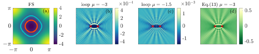
Figure 2: Twin impurity QPI for a single-pocket chiral SC ($\Delta=0.05$, $\omega=1.1\Delta$, $d=16$). (a) Band dispersion $\epsilon(\mathbf{k})=-2(\cos k_{x}+\cos k_{y})$ (denoted by color) and the FS at $\mu=-3$ (red line) and $\mu=-1.5$ (blue line) in the first Brillouin zone. (b), (c) Twin non-magnetic impurity loop contribution for $p+ip$-wave pairing with $\mu=-3$ and $\mu=-1.5$. (d) A plot of our analytical expression (Eq. (13)) for the loop contribution (in arbitrary unit) on a $81\times 81$ real space lattice with $\mu=-3$ shows the expected agreement with the corresponding numerical results presented in panel (b).

Chiral SC.— While some aspects of the HF signal for the $s$-wave minimal model above carry over to chiral pairing symmetries, the twin QPI pattern of a chiral SC already exhibits an HF signal for non-magnetic impurities. Picking $\Delta_{\mathbf{k}}^{p}=\Delta(\sin k_{x}+i\sin k_{y})$ for illustration, we find ${G}_{{0}}$ according to Eq. (9) along with

$$F_{0}^{p}(\mathbf{r})=(\tilde{F}_{0}^{p}\left(\mathbf{r}\right))^{\star}\sim\frac{i\tilde{\Delta}}{\omega^{\prime}}r^{-1/2}\sin r\ e^{i\theta},$$ (12)

where $\theta$ is the polar angle of $\mathbf{r}$. This gives a loop contribution to the LDOS according to

$$N_{p}^{\text{loop }}(\mathbf{r})\sim\left(r_{1}r_{2}d\right)^{-1/2}\times\left\{\cos\left(r_{1}+r_{2}+d\right)+\right.$$ (13)

$$\frac{{\Delta}^{2}}{\omega^{\prime 2}}\left[\sin r_{1}\sin r_{2}\cos d\cos\left(\theta_{1}-\theta_{2}\right)+\cos r_{1}\cos r_{2}\cos d\right.$$

$$\left.\pm(\cos r_{1}\sin r_{2}\sin d\cos\theta_{2}-\sin r_{1}\cos r_{2}\sin d\cos\theta_{1})]\right\},$$

where $\theta_{1}$ and $\theta_{2}$ denote the polar angle of $\mathbf{r}-\mathbf{r}_{1}$ and $\mathbf{r}-\mathbf{r}_{2}$, respectively, and $+$/$-$ corresponds to NM/M impurities. According to trigonometric transformations, we immediately recognize that Eq. (13) is also the summation of the oscillations of $r_{1}+r_{2}$ and of $r_{1}-r_{2}$, albeit the amplitude is further modulated by terms related to the polar angles $\theta_{1}$ and $\theta_{2}$. That is why we also see HF on top of elliptical fringes in Fig. 2 (b). We employ Eq. (13) in Fig. 2 (d) to compare our analytical approximation against the numerical calculation in Fig. 2 (b), which shows good agreement. In contrast to the uniform $s$-wave pairing, here the two scattering processes $\mathbf{r}\rightarrow\mathbf{r}_{1}\rightarrow\mathbf{r}_{2}\rightarrow\mathbf{r}$ and $\mathbf{r}\rightarrow\mathbf{r}_{2}\rightarrow\mathbf{r}_{1}\rightarrow\mathbf{r}$, which are time-reversed to each other, can also interfere to generate the HF, as the superconducting gaps acquire different winding phases on the two paths. This interference is reflected in the $\cos\left(\theta_{1}-\theta_{2}\right)$ term in Eq. (13). We further study the HF signal for a $d+id$-wave SC and find the overall pattern to be similar to that of the $p+ip$-wave case (see SM). The crucial difference is that the interference pattern in the region between two impurity sites for the $d+id$-wave pairing is not uniform but stripe-like, which is attributed to the distinct phase winding of two SC orders and can be explained from their detailed analytic form (details in SM). For magnetic impurities, the interference patterns are similar, as detailed in the SM.

Note that for our analytical expressions Eq. (11) and (13) we have assumed $\eta\rightarrow 0^{+}$, while in numerical calculations $\eta$ has to take a non-zero value (which we have chosen as $\eta=5\times 10^{-3}$). Having a non-zero $\eta$ regulator just amounts to setting $\omega\rightarrow\omega+i\eta$ in Eq. (9), (10) and (12), and does not affect the main features of the LDOS distribution. Departing from the band edge limit where we can compare against our analytical solution, we find that the numerical HF signature prevails even for non-circular Fermi surfaces (Fig. 2 (c)). This allows to conjecture that the HF pattern is a generic signal for twin-impurity QPI patterns of chiral SCs, where the HF signal dependence on the chemical potential is further detailed in sup .

$s_{\pm}$-wave in multi-pocket systems.— Multi-pocket Fermiologies can qualitatively differ from single-pocket systems. In particular, with respect to gapped SCs, multi-pocket systems can exhibit $s_{\pm}$-wave unconventional pairing where the gap function takes opposite signs on different Fermi pockets Hanaguri et al. (2010). We start from a two-band model for iron-based SC (Sykora and Coleman (2011))

$$H= \sum_{\mathbf{k},\sigma}\left(\varepsilon_{\mathbf{k}}^{c}c_{\mathbf{k},\sigma}^{\dagger}c_{\mathbf{k},\sigma}+\varepsilon_{\mathbf{k}}^{d}d_{\mathbf{k},\sigma}^{\dagger}d_{\mathbf{k},\sigma}\right)$$ (14)

$$+\sum_{\mathbf{k}}\left[\Delta_{\mathbf{k}}\left(c_{\mathbf{k},\uparrow}c_{-\mathbf{k},\downarrow}+d_{\mathbf{k},\uparrow}d_{-\mathbf{k},\downarrow}\right)+\text{h.c.}\right].$$

Here, “c” and “d” label the two electron bands describing an electron-like FS centered at the M point in the folded Brillouin zone (or $(\pi,0)/(0,\pi)$ for the unfolded zone Ding et al. (2008)) and a hole-like FS at the $\Gamma$ point. It reads

$$\varepsilon_{\mathbf{k}}^{c}=2t\left[\cos\left(k_{x}+k_{y}\right)+\cos\left(k_{x}-k_{y}\right)\right]-\mu_{c},$$ (15)

$$\varepsilon_{\mathbf{k}}^{d}=2t\left(\cos k_{x}+\cos k_{y}\right)-\mu_{d},$$ (16)

where we choose $\mu_{c}=-3.2$ and $\mu_{d}=3.6$ (Fig. 3(a)). It turns out that $s_{\pm}$-wave order, as opposed to conventional $s$-wave order without a sign-changing order parameter, exhibits an HF signal for any kind of impurity. Consider two types of $s$-wave pairing

$$\Delta_{\mathbf{k}}=\left\{\begin{array}[]{lr}\Delta_{s},&\ s\textrm{-wave}\\ \Delta_{s_{\pm}}\cos k_{x}\cos k_{y},&\ s_{\pm}\textrm{-wave}\end{array}\right.$$ (17)

where $t=1$, $\Delta_{s}=0.32$, and $\Delta_{s_{\pm}}=0.4$. The extended $s$-wave pairing gives the same gap magnitude but takes opposite signs on the two FS of the two electron bands.

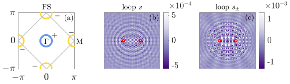
Figure 3: Twin impurity QPI for multi-pocket $s_{\pm}$-wave SC ($\omega=0.3232$, $d=24$). (a) FS of the “c” (denoted by yellow line) and the “d” (denoted by blue line) electron bands of a two-band model. $+$ ($-$) denote the sign of the gap for $s_{\pm}$-wave pairing. (b) Loop contribution from two non-magnetic impurities for conventional on-site $s$-wave pairing around two non-magnetic impurities. (c) Loop contribution as in (b) for $s_{\pm}$-wave pairing.

The formalism laid out for the single pocket case readily generalizes to the two-band model by recognizing $\mathbf{G}_{{0}}\left(\mathbf{r}\right)=\mathbf{G}^{c}_{{0}}\left(\mathbf{r}\right)+\mathbf{G}^{d}_{{0}}\left(\mathbf{r}\right)$, where $\mathbf{G}^{c}_{{0}}\left(\mathbf{r}\right)$ and $\mathbf{G}^{d}_{{0}}\left(\mathbf{r}\right)$ are defined via Eq. (4) (the unfolded Brillouin zone is used to perform the summation in the Fourier transformation) and Eqs. (15)-(17). In Fig. 3 (b) and (c), we show the loop contribution in the LDOS distribution of the two-band SC around two non-magnetic impurities for conventional $s$-wave pairing and unconventional $s_{\pm}$-wave pairing, respectively. For Fig. 3 (c), a uniform gap ($\tilde{\Delta}=0.32$) with opposite sign on the two electron bands is used in the underlying calculation in order to reduce the gap anisotropy. Similar to our previous results for conventional $s$-wave pairing on a single pocket, the loop contribution results in elliptical fringes. In addition, however, an extended $s_{\pm}$-wave SC order parameter gives rise to the emergence of HF signal on top of the ellipses. We note that the emergence of HF is due to the fact that a sign-reversing scattering at a non-magnetic impurity is mathematically equivalent to a sign-preserving scattering at a magnetic impurity. As we have shown for single-pocket $s$-wave SC, the latter case can generate HF. The “Mosaic”-like feature (zigzag between neighboring sites) is due to the FS of the electron-like band centering at the M point. Since the FS of the two band model is well approximated by circles, the formulas Eq. (8)-(10) carry over to the two-band case and analytically explain the HF signal difference between conventional and unconventional $s$-wave pairing sup . The latter distinguishability only holds for non-magnetic impurities, as magnetic impurities imply HF pattern in both cases. Our findings for the two-pocket case with sign-changing should generalize to the generic multi-pocket case with sign-changing gap function on individual pockets.

Experimental detectability.— The loop contribution is generally smaller than the single contribution according to $N^{\text{loop}}/N^{\text{single}}\sim(k_{F}d)^{-1/2}U_{0}/t$ for non-magnetic impurities. Thus, it is crucial to isolate the loop contribution in STM measurements from the single contribution background, a procedure for which we provide two proposals. The first option involves measuring the LDOS around a single impurity before measuring close to twin impurities. By subtracting the single-impurity contribution from the full contribution, the loop contribution can be isolated. Our second proposal is specifically designed for magnetic impurities, where two measurements are made with the twin impurities with anti-aligned and aligned magnetic moments. While this change does not affect the individual contributions (second order), the loop signal changes sign between the configurations. Taking the difference between the two signals thus significantly suppresses the single contribution and singles out the loop contribution. In the SM, we provide detailed simulations demonstrating the effectiveness of these proposals. In the measurements, such twin impurities might be fabricated through STM atomic manipulation Hla (2014), which would further allow to explore the evolution of the HF pattern as a function of twin impurity. A simple proof-of-principle experiment for our predicted HF pattern appears to be a conventional $s$-wave superconductor with a clean surface and highly adjustable magnetic impurities on top of it. A good candidate is NbSe₂, which can be grown by molecular beam epitaxy yielding clean surfaces Ugeda et al. (2016) required for quasiparticle interference experiments Arguello et al. (2015). Moreover, with their $s_{\pm}$-wave pairing, it is also promising to examine the HF signal in iron-based superconductors such as LiFeAs Allan et al. (2012); Platt et al. (2011).

Conclusion and outlook.— The hyperbolic fringe (HF) pattern from twin impurity QPI provides a complementary approach of detecting phase information associated with SC order. While conventional pairing necessitates magnetic twin impurities to generate an HF signal, chiral SC and $s_{\pm}$-wave multi-pocket SC already exhibit HF signal for non-magnetic impurities. Upon closer inspection of the principal underlying mathematical structure, it is apparent that the HF signal is not special to SC, but can potentially appear in entirely different contexts such as topological insulators (TIs). For instance, the Qi-Wu-Zhang model on a two-dimensional lattice (Qi et al. (2006)) for time-reversal symmetry breaking TIs exhibits a k-space Hamiltonian that has the same form as a chiral $p$-wave SC. It is hence plausible that the HF signature of twin impurities should also appear in the loop contribution to the TI LDOS distribution in the topologically non-trivial regime. For other TIs and topological materials such as graphene, the QPI pattern on the surface around twin impurities presents itself as a valuable perspective for future study.

Acknowledgments.— R.T. thanks his mentor and friend Shoucheng Zhang for a discussion which has provided the inspiration for this project. This work is funded by the Deutsche Forschungsgemeinschaft (DFG, German Research Foundation) through Project-ID 258499086 - SFB 1170 and through the Würzburg-Dresden Cluster of Excellence on Complexity and Topology in Quantum Matter - ct.qmat Project-ID 390858490 - EXC 2147. This work is also supported by the Singapore National Research Foundation QEP grant (Grant No. NRF2021-QEP2-02-P09).

References

- Byers et al. (1993) J. M. Byers, M. E. Flatté, and D. J. Scalapino, Physical Review Letters 71, 3363 (1993).
- Hoffman et al. (2002) J. E. Hoffman, E. W. Hudson, K. M. Lang, V. Madhavan, H. Eisaki, S. Uchida, and J. C. Davis, Science 295, 466 (2002).
- Wang and Lee (2003) Q.-H. Wang and D.-H. Lee, Physical Review B 67, 020511 (2003).
- Hanaguri et al. (2010) T. Hanaguri, S. Niitaka, K. Kuroki, and H. Takagi, Science 328, 474 (2010).
- Sykora and Coleman (2011) S. Sykora and P. Coleman, Physical Review B 84, 054501 (2011).
- Zheng and Hasan (2018) H. Zheng and M. Z. Hasan, Advances in Physics: X 3, 1466661 (2018).
- Akbari et al. (2010) A. Akbari, J. Knolle, I. Eremin, and R. Moessner, Phys. Rev. B 82, 224506 (2010).
- Bena (2016) C. Bena, Comptes Rendus Physique 17, 302 (2016), physique de la matière condensée au XXIe siècle: l’héritage de Jacques Friedel.
- Roushan et al. (2009) P. Roushan, J. Seo, C. V. Parker, Y. S. Hor, D. Hsieh, D. Qian, A. Richardella, M. Z. Hasan, R. J. Cava, and A. Yazdani, Nature 460, 1106 (2009).
- Lee et al. (2009) W.-C. Lee, C. Wu, D. P. Arovas, and S.-C. Zhang, Physical Review B 80, 245439 (2009).
- Balatsky et al. (2006) A. V. Balatsky, I. Vekhter, and J.-X. Zhu, Rev. Mod. Phys. 78, 373 (2006).
- Yu (1965) L. Yu, - Acta Physica Sinica - 21, (1965).
- Mashkoori et al. (2017) M. Mashkoori, K. Björnson, and A. M. Black-Schaffer, Scientific Reports 7, 44107 (2017).
- Queiroz and Stern (2018) R. Queiroz and A. Stern, Phys. Rev. Lett. 121, 176401 (2018).
- Flatté and Reynolds (2000) M. E. Flatté and D. E. Reynolds, Physical Review B 61, 14810 (2000).
- Morr and Stavropoulos (2003) D. K. Morr and N. A. Stavropoulos, Physical Review B 67, 020502 (2003).
- Choi (2004) C. H. Choi, Journal of the Korean Physical Society 44, 355 (2004).
- Zhu et al. (2003) L. Zhu, W. A. Atkinson, and P. J. Hirschfeld, Physical Review B 67, 094508 (2003).
- Cano and Paul (2009) A. Cano and I. Paul, Physical Review B 80, 153401 (2009).
- Ortuzar et al. (2022) J. Ortuzar, S. Trivini, M. Alvarado, M. Rouco, J. Zaldivar, A. L. Yeyati, J. I. Pascual, and F. S. Bergeret, Phys. Rev. B 105, 245403 (2022).
- Pustogow et al. (2019) A. Pustogow, Y. Luo, A. Chronister, Y. S. Su, D. A. Sokolov, F. Jerzembeck, A. P. Mackenzie, C. W. Hicks, N. Kikugawa, S. Raghu, E. D. Bauer, and S. E. Brown, Nature 574, 72 (2019).
- Kiesel et al. (2013) M. L. Kiesel, C. Platt, W. Hanke, and R. Thomale, Phys. Rev. Lett. 111, 097001 (2013).
- Wolf et al. (2022) S. Wolf, D. Di Sante, T. Schwemmer, R. Thomale, and S. Rachel, Phys. Rev. Lett. 128, 167002 (2022).
- Neupert et al. (2022) T. Neupert, M. M. Denner, J.-X. Yin, R. Thomale, and M. Z. Hasan, Nature Physics 18, 137 (2022).
- Stewart (2011) G. R. Stewart, Rev. Mod. Phys. 83, 1589 (2011).
- (26) Supplementary material, including references Pientka et al. (2013); Machida et al. (2019).
- (27) By performing Fourier transformation in the first Brillouin zone via Eq. 4, and through using Eqs. 8, 3, we obtain a numerical estimate for LDOS distribution. We focus on the regime where the energy bias of the STM tip is slightly above the bulk gap. The strength of impurities is chosen as the typical value (of the magnitude of hundred meV)(Wang and Lee (2003)). In actual calculations, a large real space lattice is needed to achieve a high momentum resolution in the Fourier transformation. In our case, we adopt the LDOS of the central plaquette within an discretization. Also, should be of the same magnitude as the numerical energy resolution, i.e. . We take .
- Ding et al. (2008) H. Ding, P. Richard, K. Nakayama, K. Sugawara, T. Arakane, Y. Sekiba, A. Takayama, S. Souma, T. Sato, T. Takahashi, Z. Wang, X. Dai, Z. Fang, G. F. Chen, J. L. Luo, and N. L. Wang, Europhysics Letters 83, 47001 (2008).
- Hla (2014) S. W. Hla, Reports on Progress in Physics 77, 056502 (2014).
- Ugeda et al. (2016) M. M. Ugeda, A. J. Bradley, Y. Zhang, S. Onishi, Y. Chen, W. Ruan, C. Ojeda-Aristizabal, H. Ryu, M. T. Edmonds, H.-Z. Tsai, A. Riss, S.-K. Mo, D. Lee, A. Zettl, Z. Hussain, Z.-X. Shen, and M. F. Crommie, Nature Physics 12, 92 (2016).
- Arguello et al. (2015) C. J. Arguello, E. P. Rosenthal, E. F. Andrade, W. Jin, P. C. Yeh, N. Zaki, S. Jia, R. J. Cava, R. M. Fernandes, A. J. Millis, T. Valla, R. M. Osgood, and A. N. Pasupathy, Phys. Rev. Lett. 114, 037001 (2015).
- Allan et al. (2012) M. P. Allan, A. W. Rost, A. P. Mackenzie, Y. Xie, J. C. Davis, K. Kihou, C. H. Lee, A. Iyo, H. Eisaki, and T.-M. Chuang, Science 336, 563 (2012).
- Platt et al. (2011) C. Platt, R. Thomale, and W. Hanke, Phys. Rev. B 84, 235121 (2011).
- Qi et al. (2006) X.-L. Qi, Y.-S. Wu, and S.-C. Zhang, Phys. Rev. B 74, 085308 (2006).
- Pientka et al. (2013) F. Pientka, L. I. Glazman, and F. von Oppen, Physical Review B 88, 155420 (2013).
- Machida et al. (2019) T. Machida, Y. Sun, S. Pyon, S. Takeda, Y. Kohsaka, T. Hanaguri, T. Sasagawa, and T. Tamegai, Nature Materials 18, 811 (2019).