Abstract
U ( 1 ) X 𝑈 subscript 1 𝑋 U(1)_{X} S U ( 3 ) C × S U ( 2 ) L × U ( 1 ) Y × U ( 1 ) X 𝑆 𝑈 subscript 3 𝐶 𝑆 𝑈 subscript 2 𝐿 𝑈 subscript 1 𝑌 𝑈 subscript 1 𝑋 SU(3)_{C}\times SU(2)_{L}\times U(1)_{Y}\times U(1)_{X} Z → l i ± l j ∓ → 𝑍 superscript subscript 𝑙 𝑖 plus-or-minus superscript subscript 𝑙 𝑗 minus-or-plus Z\rightarrow{{l_{i}}^{\pm}{l_{j}}^{\mp}} Z → e μ → 𝑍 𝑒 𝜇 Z\rightarrow e{\mu} Z → e τ → 𝑍 𝑒 𝜏 Z\rightarrow e{\tau} Z → μ τ → 𝑍 𝜇 𝜏 Z\rightarrow{\mu}{\tau} h → l i ± l j ∓ → ℎ superscript subscript 𝑙 𝑖 plus-or-minus superscript subscript 𝑙 𝑗 minus-or-plus h\rightarrow{{l_{i}}^{\pm}{l_{j}}^{\mp}} h → e μ → ℎ 𝑒 𝜇 h\rightarrow e{\mu} h → e τ → ℎ 𝑒 𝜏 h\rightarrow e{\tau} h → μ τ → ℎ 𝜇 𝜏 h\rightarrow{\mu}{\tau} Z → l i ± l j ∓ → 𝑍 superscript subscript 𝑙 𝑖 plus-or-minus superscript subscript 𝑙 𝑗 minus-or-plus Z\rightarrow{{l_{i}}^{\pm}{l_{j}}^{\mp}} 10 − 9 superscript 10 9 10^{-9} 10 − 13 superscript 10 13 10^{-13} h → l i ± l j ∓ → ℎ superscript subscript 𝑙 𝑖 plus-or-minus superscript subscript 𝑙 𝑗 minus-or-plus h\rightarrow{{l_{i}}^{\pm}{l_{j}}^{\mp}} 10 − 3 superscript 10 3 10^{-3} 10 − 9 superscript 10 9 10^{-9}
I Introduction
Neutrinos have tiny masses and mix with each other, as proved by the neutrino oscillation experimentIN0 ; IN1 IN2 ; IN3
In Table I, we summarize the current limitations and future prospects
of the three modes of Z boson (Z → e μ → 𝑍 𝑒 𝜇 Z\rightarrow e{\mu} Z → e τ → 𝑍 𝑒 𝜏 Z\rightarrow e{\tau} Z → μ τ → 𝑍 𝜇 𝜏 Z\rightarrow{\mu}{\tau} T7 ; T3 ; T8 ; T9 ; T4 ; T5 5 × 10 6 5 superscript 10 6 5\times 10^{6} e + e − superscript 𝑒 superscript 𝑒 e^{+}e^{-} T7 7.8 × 10 8 7.8 superscript 10 8 7.8\times 10^{8} T7 e + e − superscript 𝑒 superscript 𝑒 e^{+}e^{-} 3 × 10 12 3 superscript 10 12 3\times 10^{12} T3 Z → e τ → 𝑍 𝑒 𝜏 Z\rightarrow e{\tau} Z → μ τ → 𝑍 𝜇 𝜏 Z\rightarrow{\mu}{\tau}
For h → l i ± l j ∓ → ℎ superscript subscript 𝑙 𝑖 plus-or-minus superscript subscript 𝑙 𝑗 minus-or-plus h\rightarrow{{l_{i}}^{\pm}{l_{j}}^{\mp}} h → e μ → ℎ 𝑒 𝜇 h\rightarrow e{\mu} h → e τ → ℎ 𝑒 𝜏 h\rightarrow e{\tau} h → μ τ → ℎ 𝜇 𝜏 h\rightarrow{\mu}{\tau} h → e μ → ℎ 𝑒 𝜇 h\rightarrow e{\mu} h → e τ → ℎ 𝑒 𝜏 h\rightarrow e{\tau} h → μ τ → ℎ 𝜇 𝜏 h\rightarrow{\mu}{\tau} h → e τ → ℎ 𝑒 𝜏 h\rightarrow e{\tau} h → μ τ → ℎ 𝜇 𝜏 h\rightarrow{\mu}{\tau} Z4 ; Z1 ; Z2 ; T6
Combining the experimental data provided by ATLAS and CMS, the upper limits on the LFV branching ratios of Z → e μ → 𝑍 𝑒 𝜇 Z\rightarrow e{\mu} Z → e τ → 𝑍 𝑒 𝜏 Z\rightarrow e{\tau} Z → μ τ → 𝑍 𝜇 𝜏 Z\rightarrow{\mu}{\tau} h → e μ → ℎ 𝑒 𝜇 h\rightarrow e{\mu} h → e τ → ℎ 𝑒 𝜏 h\rightarrow e{\tau} h → μ τ → ℎ 𝜇 𝜏 h\rightarrow{\mu}{\tau} 3 Z3 ; IN4 ; IN5 ; IN6 ; IN7 Z8 ; Z46 Z13 ; Z14 ; Z15 ; Z16 ; Z17 ; Z18
Table 1: Current upper limits on LFV Z decays from LEP and LHC experiments and future sensitivity from CEPC/FCC-ee
Table 2: Current upper limits and future sensitivity on LFV Higgs decays
U ( 1 ) X 𝑈 subscript 1 𝑋 U(1)_{X} S U ( 3 ) C × S U ( 2 ) L × U ( 1 ) Y × U ( 1 ) X 𝑆 𝑈 subscript 3 𝐶 𝑆 𝑈 subscript 2 𝐿 𝑈 subscript 1 𝑌 𝑈 subscript 1 𝑋 SU(3)_{C}\times SU(2)_{L}\times U(1)_{Y}\times U(1)_{X} Sarah1 ; Sarah2 ; Sarah3 Z → l i ± l j ∓ → 𝑍 superscript subscript 𝑙 𝑖 plus-or-minus superscript subscript 𝑙 𝑗 minus-or-plus Z\rightarrow{{l_{i}}^{\pm}{l_{j}}^{\mp}} Z → e μ → 𝑍 𝑒 𝜇 Z\rightarrow e{\mu} Z → e τ → 𝑍 𝑒 𝜏 Z\rightarrow e{\tau} Z → μ τ → 𝑍 𝜇 𝜏 Z\rightarrow{\mu}{\tau} h → l i ± l j ∓ → ℎ superscript subscript 𝑙 𝑖 plus-or-minus superscript subscript 𝑙 𝑗 minus-or-plus h\rightarrow{{l_{i}}^{\pm}{l_{j}}^{\mp}} h → e μ → ℎ 𝑒 𝜇 h\rightarrow e{\mu} h → e τ → ℎ 𝑒 𝜏 h\rightarrow e{\tau} h → μ τ → ℎ 𝜇 𝜏 h\rightarrow{\mu}{\tau} U ( 1 ) X 𝑈 subscript 1 𝑋 U(1)_{X} U ( 1 ) X 𝑈 subscript 1 𝑋 U(1)_{X}
In our previous work, we study the LFV decays l j → l i γ → subscript 𝑙 𝑗 subscript 𝑙 𝑖 𝛾 l_{j}\rightarrow{l_{i}\gamma} U ( 1 ) X 𝑈 subscript 1 𝑋 U(1)_{X} T1 l j → l i γ → subscript 𝑙 𝑗 subscript 𝑙 𝑖 𝛾 l_{j}\rightarrow{l_{i}\gamma} U ( 1 ) X 𝑈 subscript 1 𝑋 U(1)_{X} l j → l i γ → subscript 𝑙 𝑗 subscript 𝑙 𝑖 𝛾 l_{j}\rightarrow{l_{i}\gamma} Z → l i ± l j ∓ → 𝑍 superscript subscript 𝑙 𝑖 plus-or-minus superscript subscript 𝑙 𝑗 minus-or-plus Z\rightarrow{{l_{i}}^{\pm}{l_{j}}^{\mp}} h → l i ± l j ∓ → ℎ superscript subscript 𝑙 𝑖 plus-or-minus superscript subscript 𝑙 𝑗 minus-or-plus h\rightarrow{{l_{i}}^{\pm}{l_{j}}^{\mp}} l j → l i γ → subscript 𝑙 𝑗 subscript 𝑙 𝑖 𝛾 l_{j}\rightarrow{l_{i}\gamma} U ( 1 ) X 𝑈 subscript 1 𝑋 U(1)_{X}
We work mainly on the following aspects. In Section II, We briefly introduce the main content of U ( 1 ) X 𝑈 subscript 1 𝑋 U(1)_{X} Z → l i ± l j ∓ → 𝑍 superscript subscript 𝑙 𝑖 plus-or-minus superscript subscript 𝑙 𝑗 minus-or-plus Z\rightarrow{{l_{i}}^{\pm}{l_{j}}^{\mp}} h → l i ± l j ∓ → ℎ superscript subscript 𝑙 𝑖 plus-or-minus superscript subscript 𝑙 𝑗 minus-or-plus h\rightarrow{{l_{i}}^{\pm}{l_{j}}^{\mp}} U ( 1 ) X 𝑈 subscript 1 𝑋 U(1)_{X}
Table 3: The upper limits on the LFV branching ratios of Z → l i ± l j ∓ → 𝑍 superscript subscript 𝑙 𝑖 plus-or-minus superscript subscript 𝑙 𝑗 minus-or-plus Z\rightarrow{{l_{i}}^{\pm}{l_{j}}^{\mp}} h → l i ± l j ∓ → ℎ superscript subscript 𝑙 𝑖 plus-or-minus superscript subscript 𝑙 𝑗 minus-or-plus h\rightarrow{{l_{i}}^{\pm}{l_{j}}^{\mp}}
II The main content of U ( 1 ) X 𝑈 subscript 1 𝑋 U(1)_{X}
U ( 1 ) X 𝑈 subscript 1 𝑋 U(1)_{X} S U ( 3 ) C ⊗ S U ( 2 ) L ⊗ U ( 1 ) Y ⊗ U ( 1 ) X tensor-product tensor-product tensor-product 𝑆 𝑈 subscript 3 𝐶 𝑆 𝑈 subscript 2 𝐿 𝑈 subscript 1 𝑌 𝑈 subscript 1 𝑋 SU(3)_{C}\otimes SU(2)_{L}\otimes U(1)_{Y}\otimes U(1)_{X} UU1 ; UU3 ; UU4 ; T1 U ( 1 ) X 𝑈 subscript 1 𝑋 U(1)_{X} ν ^ i subscript ^ 𝜈 𝑖 \hat{\nu}_{i} η ^ , η ¯ ^ , S ^ ^ 𝜂 ^ ¯ 𝜂 ^ 𝑆
\hat{\eta},~{}\hat{\bar{\eta}},~{}\hat{S} H u , H d , η , η ¯ subscript 𝐻 𝑢 subscript 𝐻 𝑑 𝜂 ¯ 𝜂
H_{u},~{}H_{d},~{}\eta,~{}\bar{\eta} S 𝑆 S 5 × 5 5 5 5\times 5 LCTHiggs1 ; LCTHiggs2 6 × 6 6 6 6\times 6
The superpotential in U ( 1 ) X 𝑈 subscript 1 𝑋 U(1)_{X}
W = l W S ^ + μ H ^ u H ^ d + M S S ^ S ^ − Y d d ^ q ^ H ^ d − Y e e ^ l ^ H ^ d + λ H S ^ H ^ u H ^ d 𝑊 subscript 𝑙 𝑊 ^ 𝑆 𝜇 subscript ^ 𝐻 𝑢 subscript ^ 𝐻 𝑑 subscript 𝑀 𝑆 ^ 𝑆 ^ 𝑆 subscript 𝑌 𝑑 ^ 𝑑 ^ 𝑞 subscript ^ 𝐻 𝑑 subscript 𝑌 𝑒 ^ 𝑒 ^ 𝑙 subscript ^ 𝐻 𝑑 subscript 𝜆 𝐻 ^ 𝑆 subscript ^ 𝐻 𝑢 subscript ^ 𝐻 𝑑 \displaystyle W=l_{W}\hat{S}+\mu\hat{H}_{u}\hat{H}_{d}+M_{S}\hat{S}\hat{S}-Y_{d}\hat{d}\hat{q}\hat{H}_{d}-Y_{e}\hat{e}\hat{l}\hat{H}_{d}+\lambda_{H}\hat{S}\hat{H}_{u}\hat{H}_{d}
+ λ C S ^ η ^ η ¯ ^ + κ 3 S ^ S ^ S ^ + Y u u ^ q ^ H ^ u + Y X ν ^ η ¯ ^ ν ^ + Y ν ν ^ l ^ H ^ u . subscript 𝜆 𝐶 ^ 𝑆 ^ 𝜂 ^ ¯ 𝜂 𝜅 3 ^ 𝑆 ^ 𝑆 ^ 𝑆 subscript 𝑌 𝑢 ^ 𝑢 ^ 𝑞 subscript ^ 𝐻 𝑢 subscript 𝑌 𝑋 ^ 𝜈 ^ ¯ 𝜂 ^ 𝜈 subscript 𝑌 𝜈 ^ 𝜈 ^ 𝑙 subscript ^ 𝐻 𝑢 \displaystyle~{}~{}~{}~{}~{}~{}+\lambda_{C}\hat{S}\hat{\eta}\hat{\bar{\eta}}+\frac{\kappa}{3}\hat{S}\hat{S}\hat{S}+Y_{u}\hat{u}\hat{q}\hat{H}_{u}+Y_{X}\hat{\nu}\hat{\bar{\eta}}\hat{\nu}+Y_{\nu}\hat{\nu}\hat{l}\hat{H}_{u}. (1)
The specific explicit expressions of two Higgs doublets are as follows:
H u = ( H u + 1 2 ( v u + H u 0 + i P u 0 ) ) , H d = ( 1 2 ( v d + H d 0 + i P d 0 ) H d − ) . formulae-sequence subscript 𝐻 𝑢 superscript subscript 𝐻 𝑢 1 2 subscript 𝑣 𝑢 superscript subscript 𝐻 𝑢 0 𝑖 superscript subscript 𝑃 𝑢 0 subscript 𝐻 𝑑 1 2 subscript 𝑣 𝑑 superscript subscript 𝐻 𝑑 0 𝑖 superscript subscript 𝑃 𝑑 0 superscript subscript 𝐻 𝑑 \displaystyle H_{u}=\left(\begin{array}[]{c}H_{u}^{+}\\
{1\over\sqrt{2}}\Big{(}v_{u}+H_{u}^{0}+iP_{u}^{0}\Big{)}\end{array}\right),~{}~{}~{}~{}~{}~{}H_{d}=\left(\begin{array}[]{c}{1\over\sqrt{2}}\Big{(}v_{d}+H_{d}^{0}+iP_{d}^{0}\Big{)}\\
H_{d}^{-}\end{array}\right). (6)
The three Higgs singlets are represented by:
η = 1 2 ( v η + ϕ η 0 + i P η 0 ) , η ¯ = 1 2 ( v η ¯ + ϕ η ¯ 0 + i P η ¯ 0 ) , formulae-sequence 𝜂 1 2 subscript 𝑣 𝜂 superscript subscript italic-ϕ 𝜂 0 𝑖 superscript subscript 𝑃 𝜂 0 ¯ 𝜂 1 2 subscript 𝑣 ¯ 𝜂 superscript subscript italic-ϕ ¯ 𝜂 0 𝑖 superscript subscript 𝑃 ¯ 𝜂 0 \displaystyle\eta={1\over\sqrt{2}}\Big{(}v_{\eta}+\phi_{\eta}^{0}+iP_{\eta}^{0}\Big{)},~{}~{}~{}~{}~{}~{}~{}~{}~{}~{}~{}~{}~{}~{}~{}\bar{\eta}={1\over\sqrt{2}}\Big{(}v_{\bar{\eta}}+\phi_{\bar{\eta}}^{0}+iP_{\bar{\eta}}^{0}\Big{)},
S = 1 2 ( v S + ϕ S 0 + i P S 0 ) . 𝑆 1 2 subscript 𝑣 𝑆 superscript subscript italic-ϕ 𝑆 0 𝑖 superscript subscript 𝑃 𝑆 0 \displaystyle\hskip 85.35826ptS={1\over\sqrt{2}}\Big{(}v_{S}+\phi_{S}^{0}+iP_{S}^{0}\Big{)}. (7)
Here, v u , v d , v η subscript 𝑣 𝑢 subscript 𝑣 𝑑 subscript 𝑣 𝜂
v_{u},~{}v_{d},~{}v_{\eta} v η ¯ subscript 𝑣 ¯ 𝜂 v_{\bar{\eta}} v S subscript 𝑣 𝑆 v_{S} H u subscript 𝐻 𝑢 H_{u} H d subscript 𝐻 𝑑 H_{d} η 𝜂 \eta η ¯ ¯ 𝜂 \bar{\eta} S 𝑆 S tan β = v u / v d 𝛽 subscript 𝑣 𝑢 subscript 𝑣 𝑑 \tan\beta=v_{u}/v_{d} tan β η = v η ¯ / v η subscript 𝛽 𝜂 subscript 𝑣 ¯ 𝜂 subscript 𝑣 𝜂 \tan\beta_{\eta}=v_{\bar{\eta}}/v_{\eta} ν ~ L subscript ~ 𝜈 𝐿 {\widetilde{\nu}}_{L} ν ~ R subscript ~ 𝜈 𝑅 {\widetilde{\nu}}_{R}
ν ~ L = 1 2 ϕ l + i 2 σ l , ν ~ R = 1 2 ϕ R + i 2 σ R . formulae-sequence subscript ~ 𝜈 𝐿 1 2 subscript italic-ϕ 𝑙 𝑖 2 subscript 𝜎 𝑙 subscript ~ 𝜈 𝑅 1 2 subscript italic-ϕ 𝑅 𝑖 2 subscript 𝜎 𝑅 \displaystyle\widetilde{\nu}_{L}=\frac{1}{\sqrt{2}}{\phi}_{l}+\frac{i}{\sqrt{2}}{\sigma}_{l},~{}~{}~{}~{}~{}~{}~{}~{}~{}~{}~{}~{}~{}~{}\widetilde{\nu}_{R}=\frac{1}{\sqrt{2}}{\phi}_{R}+\frac{i}{\sqrt{2}}{\sigma}_{R}. (8)
The soft SUSY breaking terms of U ( 1 ) X 𝑈 subscript 1 𝑋 U(1)_{X}
ℒ s o f t = ℒ s o f t M S S M − B S S 2 − L S S − T κ 3 S 3 − T λ C S η η ¯ + ϵ i j T λ H S H d i H u j subscript ℒ 𝑠 𝑜 𝑓 𝑡 superscript subscript ℒ 𝑠 𝑜 𝑓 𝑡 𝑀 𝑆 𝑆 𝑀 subscript 𝐵 𝑆 superscript 𝑆 2 subscript 𝐿 𝑆 𝑆 subscript 𝑇 𝜅 3 superscript 𝑆 3 subscript 𝑇 subscript 𝜆 𝐶 𝑆 𝜂 ¯ 𝜂 subscript italic-ϵ 𝑖 𝑗 subscript 𝑇 subscript 𝜆 𝐻 𝑆 superscript subscript 𝐻 𝑑 𝑖 superscript subscript 𝐻 𝑢 𝑗 \displaystyle\mathcal{L}_{soft}=\mathcal{L}_{soft}^{MSSM}-B_{S}S^{2}-L_{S}S-\frac{T_{\kappa}}{3}S^{3}-T_{\lambda_{C}}S\eta\bar{\eta}+\epsilon_{ij}T_{\lambda_{H}}SH_{d}^{i}H_{u}^{j}
− T X I J η ¯ ν ~ R ∗ I ν ~ R ∗ J + ϵ i j T ν I J H u i ν ~ R I ∗ l ~ j J − m η 2 | η | 2 − m η ¯ 2 | η ¯ | 2 − m S 2 S 2 superscript subscript 𝑇 𝑋 𝐼 𝐽 ¯ 𝜂 superscript subscript ~ 𝜈 𝑅 absent 𝐼 superscript subscript ~ 𝜈 𝑅 absent 𝐽 subscript italic-ϵ 𝑖 𝑗 subscript superscript 𝑇 𝐼 𝐽 𝜈 superscript subscript 𝐻 𝑢 𝑖 superscript subscript ~ 𝜈 𝑅 𝐼
superscript subscript ~ 𝑙 𝑗 𝐽 superscript subscript 𝑚 𝜂 2 superscript 𝜂 2 superscript subscript 𝑚 ¯ 𝜂 2 superscript ¯ 𝜂 2 superscript subscript 𝑚 𝑆 2 superscript 𝑆 2 \displaystyle\hskip 42.67912pt-T_{X}^{IJ}\bar{\eta}\tilde{\nu}_{R}^{*I}\tilde{\nu}_{R}^{*J}+\epsilon_{ij}T^{IJ}_{\nu}H_{u}^{i}\tilde{\nu}_{R}^{I*}\tilde{l}_{j}^{J}-m_{\eta}^{2}|\eta|^{2}-m_{\bar{\eta}}^{2}|\bar{\eta}|^{2}-m_{S}^{2}S^{2}
− ( m ν ~ R 2 ) I J ν ~ R I ∗ ν ~ R J − 1 2 ( M X λ X ~ 2 + 2 M B B ′ λ B ~ λ X ~ ) + h . c . formulae-sequence superscript superscript subscript 𝑚 subscript ~ 𝜈 𝑅 2 𝐼 𝐽 superscript subscript ~ 𝜈 𝑅 𝐼
superscript subscript ~ 𝜈 𝑅 𝐽 1 2 subscript 𝑀 𝑋 subscript superscript 𝜆 2 ~ 𝑋 2 subscript 𝑀 𝐵 superscript 𝐵 ′ subscript 𝜆 ~ 𝐵 subscript 𝜆 ~ 𝑋 ℎ 𝑐 \displaystyle\hskip 42.67912pt-(m_{\tilde{\nu}_{R}}^{2})^{IJ}\tilde{\nu}_{R}^{I*}\tilde{\nu}_{R}^{J}-\frac{1}{2}\Big{(}M_{X}\lambda^{2}_{\tilde{X}}+2M_{BB^{\prime}}\lambda_{\tilde{B}}\lambda_{\tilde{X}}\Big{)}+h.c~{}~{}. (9)
The Table 4 U ( 1 ) X 𝑈 subscript 1 𝑋 U(1)_{X} U ( 1 ) X 𝑈 subscript 1 𝑋 U(1)_{X} UU4 U ( 1 ) Y 𝑈 subscript 1 𝑌 U(1)_{Y} U ( 1 ) X 𝑈 subscript 1 𝑋 U(1)_{X} U ( 1 ) X 𝑈 subscript 1 𝑋 U(1)_{X}
Table 4: The superfields in U ( 1 ) X 𝑈 subscript 1 𝑋 U(1)_{X}
Superfields
q ^ i subscript ^ 𝑞 𝑖 \hskip 2.84544pt\hat{q}_{i}\hskip 2.84544pt u ^ i c subscript superscript ^ 𝑢 𝑐 𝑖 \hat{u}^{c}_{i} d ^ i c subscript superscript ^ 𝑑 𝑐 𝑖 \hskip 5.69046pt\hat{d}^{c}_{i}\hskip 5.69046pt l ^ i subscript ^ 𝑙 𝑖 \hat{l}_{i} e ^ i c subscript superscript ^ 𝑒 𝑐 𝑖 \hskip 5.69046pt\hat{e}^{c}_{i}\hskip 5.69046pt ν ^ i subscript ^ 𝜈 𝑖 \hat{\nu}_{i} H ^ u subscript ^ 𝐻 𝑢 \hskip 2.84544pt\hat{H}_{u}\hskip 2.84544pt H ^ d subscript ^ 𝐻 𝑑 \hat{H}_{d} η ^ ^ 𝜂 \hskip 5.69046pt\hat{\eta}\hskip 5.69046pt η ¯ ^ ^ ¯ 𝜂 \hskip 5.69046pt\hat{\bar{\eta}}\hskip 5.69046pt S ^ ^ 𝑆 \hskip 5.69046pt\hat{S}\hskip 5.69046pt
S U ( 3 ) C 𝑆 𝑈 subscript 3 𝐶 SU(3)_{C} 3
3 ¯ ¯ 3 \bar{3} 3 ¯ ¯ 3 \bar{3} 1
1
1
1
1
1
1
1
S U ( 2 ) L 𝑆 𝑈 subscript 2 𝐿 SU(2)_{L} 2
1
1
2
1
1
2
2
1
1
1
U ( 1 ) Y 𝑈 subscript 1 𝑌 U(1)_{Y} 1/6
-2/3
1/3
-1/2
1
0
1/2
-1/2
0
0
0
U ( 1 ) X 𝑈 subscript 1 𝑋 U(1)_{X} 0
-1/2
1/2
0
1/2
-1/2
1/2
-1/2
-1
1
0
The general form of the covariant derivative of U ( 1 ) X 𝑈 subscript 1 𝑋 U(1)_{X} UMSSM5 ; B-L1 ; B-L2 ; gaugemass U ( 1 ) X 𝑈 subscript 1 𝑋 U(1)_{X} A μ X , A μ Y subscript superscript 𝐴 𝑋 𝜇 subscript superscript 𝐴 𝑌 𝜇
A^{X}_{\mu},~{}A^{Y}_{\mu} V μ 3 subscript superscript 𝑉 3 𝜇 V^{3}_{\mu} ( A μ Y , V μ 3 , A μ X ) subscript superscript 𝐴 𝑌 𝜇 subscript superscript 𝑉 3 𝜇 subscript superscript 𝐴 𝑋 𝜇 (A^{Y}_{\mu},V^{3}_{\mu},A^{X}_{\mu}) UU4 θ W subscript 𝜃 𝑊 \theta_{W} θ W ′ superscript subscript 𝜃 𝑊 ′ \theta_{W}^{\prime} θ W subscript 𝜃 𝑊 \theta_{W} θ W ′ superscript subscript 𝜃 𝑊 ′ \theta_{W}^{\prime}
sin 2 θ W ′ = 1 2 − [ ( g Y X + g X ) 2 − g 1 2 − g 2 2 ] v 2 + 4 g X 2 ξ 2 2 [ ( g Y X + g X ) 2 + g 1 2 + g 2 2 ] 2 v 4 + 8 g X 2 [ ( g Y X + g X ) 2 − g 1 2 − g 2 2 ] v 2 ξ 2 + 16 g X 4 ξ 4 . superscript 2 superscript subscript 𝜃 𝑊 ′ 1 2 delimited-[] superscript subscript 𝑔 𝑌 𝑋 subscript 𝑔 𝑋 2 superscript subscript 𝑔 1 2 superscript subscript 𝑔 2 2 superscript 𝑣 2 4 superscript subscript 𝑔 𝑋 2 superscript 𝜉 2 2 superscript delimited-[] superscript subscript 𝑔 𝑌 𝑋 subscript 𝑔 𝑋 2 superscript subscript 𝑔 1 2 superscript subscript 𝑔 2 2 2 superscript 𝑣 4 8 superscript subscript 𝑔 𝑋 2 delimited-[] superscript subscript 𝑔 𝑌 𝑋 subscript 𝑔 𝑋 2 superscript subscript 𝑔 1 2 superscript subscript 𝑔 2 2 superscript 𝑣 2 superscript 𝜉 2 16 superscript subscript 𝑔 𝑋 4 superscript 𝜉 4 \displaystyle\sin^{2}\theta_{W}^{\prime}\!=\!\frac{1}{2}\!-\!\frac{[(g_{{YX}}+g_{X})^{2}-g_{1}^{2}-g_{2}^{2}]v^{2}+4g_{X}^{2}\xi^{2}}{2\sqrt{[(g_{{YX}}+g_{X})^{2}+g_{1}^{2}+g_{2}^{2}]^{2}v^{4}\!+\!8g_{X}^{2}[(g_{{YX}}+g_{X})^{2}\!-\!g_{1}^{2}\!-\!g_{2}^{2}]v^{2}\xi^{2}\!+\!16g_{X}^{4}\xi^{4}}}. (10)
Here, v 2 = v u 2 + v d 2 superscript 𝑣 2 superscript subscript 𝑣 𝑢 2 superscript subscript 𝑣 𝑑 2 v^{2}=v_{u}^{2}+v_{d}^{2} ξ 2 = v η 2 + v η ¯ 2 superscript 𝜉 2 superscript subscript 𝑣 𝜂 2 superscript subscript 𝑣 ¯ 𝜂 2 \xi^{2}=v_{\eta}^{2}+v_{\bar{\eta}}^{2}
The new mixing angle appears in the couplings involving Z 𝑍 Z Z ′ superscript 𝑍 ′ Z^{\prime}
m γ 2 = 0 , superscript subscript 𝑚 𝛾 2 0 \displaystyle m_{\gamma}^{2}=0,
m Z , Z ′ 2 = 1 8 ( [ g 1 2 + g 2 2 + ( g Y X + g X ) 2 ] v 2 + 4 g X 2 ξ 2 \displaystyle m_{Z,{Z^{{}^{\prime}}}}^{2}=\frac{1}{8}\Big{(}[g_{1}^{2}+g_{2}^{2}+(g_{{YX}}+g_{X})^{2}]v^{2}+4g_{X}^{2}\xi^{2}
∓ [ g 1 2 + g 2 2 + ( g Y X + g X ) 2 ] 2 v 4 + 8 [ ( g Y X + g X ) 2 − g 1 2 − g 2 2 ] g X 2 v 2 ξ 2 + 16 g X 4 ξ 4 ) . \displaystyle\hskip 31.2982pt\mp\sqrt{[g_{1}^{2}+g_{2}^{2}+(g_{{YX}}+g_{X})^{2}]^{2}v^{4}\!+\!8[(g_{{YX}}+g_{X})^{2}\!-\!g_{1}^{2}\!-\!g_{2}^{2}]g_{X}^{2}v^{2}\xi^{2}\!+\!16g_{X}^{4}\xi^{4}}\Big{)}. (11)
The mass squared matrix for CP-even Higgs ( ϕ d , ϕ u , ϕ η , ϕ η ¯ , ϕ s ) subscript italic-ϕ 𝑑 subscript italic-ϕ 𝑢 subscript italic-ϕ 𝜂 subscript italic-ϕ ¯ 𝜂 subscript italic-ϕ 𝑠 ({\phi}_{d},{\phi}_{u},{\phi}_{\eta},{\phi}_{\overline{\eta}},{\phi}_{s})
M h 2 = ( m ϕ d ϕ d m ϕ u ϕ d m ϕ η ϕ d m ϕ η ¯ ϕ d m ϕ s ϕ d m ϕ d ϕ u m ϕ u ϕ u m ϕ η ϕ u m ϕ η ¯ ϕ u m ϕ s ϕ u m ϕ d ϕ η m ϕ u ϕ η m ϕ η ϕ η m ϕ η ¯ ϕ η m ϕ s ϕ η m ϕ d ϕ η ¯ m ϕ u ϕ η ¯ m ϕ η ϕ η ¯ m ϕ η ¯ ϕ η ¯ m ϕ s ϕ η ¯ m ϕ d ϕ s m ϕ u ϕ s m ϕ η ϕ s m ϕ η ¯ ϕ s m ϕ s ϕ s ) , subscript superscript 𝑀 2 ℎ subscript 𝑚 subscript italic-ϕ 𝑑 subscript italic-ϕ 𝑑 subscript 𝑚 subscript italic-ϕ 𝑢 subscript italic-ϕ 𝑑 subscript 𝑚 subscript italic-ϕ 𝜂 subscript italic-ϕ 𝑑 subscript 𝑚 subscript italic-ϕ ¯ 𝜂 subscript italic-ϕ 𝑑 subscript 𝑚 subscript italic-ϕ 𝑠 subscript italic-ϕ 𝑑 subscript 𝑚 subscript italic-ϕ 𝑑 subscript italic-ϕ 𝑢 subscript 𝑚 subscript italic-ϕ 𝑢 subscript italic-ϕ 𝑢 subscript 𝑚 subscript italic-ϕ 𝜂 subscript italic-ϕ 𝑢 subscript 𝑚 subscript italic-ϕ ¯ 𝜂 subscript italic-ϕ 𝑢 subscript 𝑚 subscript italic-ϕ 𝑠 subscript italic-ϕ 𝑢 subscript 𝑚 subscript italic-ϕ 𝑑 subscript italic-ϕ 𝜂 subscript 𝑚 subscript italic-ϕ 𝑢 subscript italic-ϕ 𝜂 subscript 𝑚 subscript italic-ϕ 𝜂 subscript italic-ϕ 𝜂 subscript 𝑚 subscript italic-ϕ ¯ 𝜂 subscript italic-ϕ 𝜂 subscript 𝑚 subscript italic-ϕ 𝑠 subscript italic-ϕ 𝜂 subscript 𝑚 subscript italic-ϕ 𝑑 subscript italic-ϕ ¯ 𝜂 subscript 𝑚 subscript italic-ϕ 𝑢 subscript italic-ϕ ¯ 𝜂 subscript 𝑚 subscript italic-ϕ 𝜂 subscript italic-ϕ ¯ 𝜂 subscript 𝑚 subscript italic-ϕ ¯ 𝜂 subscript italic-ϕ ¯ 𝜂 subscript 𝑚 subscript italic-ϕ 𝑠 subscript italic-ϕ ¯ 𝜂 subscript 𝑚 subscript italic-ϕ 𝑑 subscript italic-ϕ 𝑠 subscript 𝑚 subscript italic-ϕ 𝑢 subscript italic-ϕ 𝑠 subscript 𝑚 subscript italic-ϕ 𝜂 subscript italic-ϕ 𝑠 subscript 𝑚 subscript italic-ϕ ¯ 𝜂 subscript italic-ϕ 𝑠 subscript 𝑚 subscript italic-ϕ 𝑠 subscript italic-ϕ 𝑠 \displaystyle M^{2}_{h}=\left(\begin{array}[]{ccccc}m_{{\phi}_{d}{\phi}_{d}}&m_{{\phi}_{u}{\phi}_{d}}&m_{{\phi}_{\eta}{\phi}_{d}}&m_{{\phi}_{\overline{\eta}}{\phi}_{d}}&m_{{\phi}_{s}{\phi}_{d}}\\
m_{{\phi}_{d}{\phi}_{u}}&m_{{\phi}_{u}{\phi}_{u}}&m_{{\phi}_{\eta}{\phi}_{u}}&m_{{\phi}_{\overline{\eta}}{\phi}_{u}}&m_{{\phi}_{s}{\phi}_{u}}\\
m_{{\phi}_{d}{\phi}_{\eta}}&m_{{\phi}_{u}{\phi}_{\eta}}&m_{{\phi}_{\eta}{\phi}_{\eta}}&m_{{\phi}_{\overline{\eta}}{\phi}_{\eta}}&m_{{\phi}_{s}{\phi}_{\eta}}\\
m_{{\phi}_{d}{\phi}_{\overline{\eta}}}&m_{{\phi}_{u}{\phi}_{\overline{\eta}}}&m_{{\phi}_{\eta}{\phi}_{\overline{\eta}}}&m_{{\phi}_{\overline{\eta}}{\phi}_{\overline{\eta}}}&m_{{\phi}_{s}{\phi}_{\overline{\eta}}}\\
m_{{\phi}_{d}{\phi}_{s}}&m_{{\phi}_{u}{\phi}_{s}}&m_{{\phi}_{\eta}{\phi}_{s}}&m_{{\phi}_{\overline{\eta}}{\phi}_{s}}&m_{{\phi}_{s}{\phi}_{s}}\end{array}\right), (17)
m ϕ d ϕ d = m H d 2 + | μ | 2 + 1 8 ( [ g 1 2 + ( g X + g Y X ) 2 + g 2 2 ] ( 3 v d 2 − v u 2 ) \displaystyle m_{\phi_{d}\phi_{d}}=m_{H_{d}}^{2}+|\mu|^{2}+\frac{1}{8}\Big{(}[g_{1}^{2}+(g_{X}+g_{YX})^{2}+g_{2}^{2}](3v_{d}^{2}-v_{u}^{2})
+ 2 ( g Y X g X + g X 2 ) ( v η 2 − v η ¯ 2 ) ) + 2 v S μ λ H + 1 2 ( v u 2 + v S 2 ) | λ H | 2 , \displaystyle\hskip 42.67912pt+2(g_{YX}g_{X}+g_{X}^{2})(v_{\eta}^{2}-v_{\bar{\eta}}^{2})\Big{)}+\sqrt{2}v_{S}\mu{\lambda}_{H}+\frac{1}{2}(v_{u}^{2}+v_{S}^{2})|{\lambda}_{H}|^{2}, (18)
m ϕ d ϕ u = − 1 4 ( g 2 2 + ( g Y X + g X ) 2 + g 1 2 ) v d v u + | λ H | 2 v d v u − λ H l W subscript 𝑚 subscript italic-ϕ 𝑑 subscript italic-ϕ 𝑢 1 4 superscript subscript 𝑔 2 2 superscript subscript 𝑔 𝑌 𝑋 subscript 𝑔 𝑋 2 superscript subscript 𝑔 1 2 subscript 𝑣 𝑑 subscript 𝑣 𝑢 superscript subscript 𝜆 𝐻 2 subscript 𝑣 𝑑 subscript 𝑣 𝑢 subscript 𝜆 𝐻 subscript 𝑙 𝑊 \displaystyle m_{\phi_{d}\phi_{u}}=-\frac{1}{4}\Big{(}g_{2}^{2}+(g_{YX}+g_{X})^{2}+g_{1}^{2}\Big{)}v_{d}v_{u}+|{\lambda}_{H}|^{2}v_{d}v_{u}-{\lambda}_{H}l_{W}
− 1 2 λ H ( v η v η ¯ λ C + v S 2 κ ) − B μ − 2 v S ( 1 2 T λ H + M S λ H ) , 1 2 subscript 𝜆 𝐻 subscript 𝑣 𝜂 subscript 𝑣 ¯ 𝜂 subscript 𝜆 𝐶 superscript subscript 𝑣 𝑆 2 𝜅 subscript 𝐵 𝜇 2 subscript 𝑣 𝑆 1 2 subscript 𝑇 subscript 𝜆 𝐻 subscript 𝑀 𝑆 subscript 𝜆 𝐻 \displaystyle\hskip 42.67912pt-\frac{1}{2}{\lambda}_{H}(v_{\eta}v_{\bar{\eta}}{\lambda}_{C}+v_{S}^{2}\kappa)-B_{\mu}-\sqrt{2}v_{S}(\frac{1}{2}T_{{\lambda}_{H}}+M_{S}{\lambda}_{H}), (19)
m ϕ u ϕ u = m H u 2 + | μ | 2 + 1 8 ( [ g 1 2 + ( g X + g Y X ) 2 + g 2 2 ] ( 3 v u 2 − v d 2 ) \displaystyle m_{\phi_{u}\phi_{u}}=m_{H_{u}}^{2}+|\mu|^{2}+\frac{1}{8}\Big{(}[g_{1}^{2}+(g_{X}+g_{YX})^{2}+g_{2}^{2}](3v_{u}^{2}-v_{d}^{2})
+ 2 ( g Y X g X + g X 2 ) ( v η ¯ 2 − v η 2 ) ) + 2 v S μ λ H + 1 2 ( v d 2 + v S 2 ) | λ H | 2 , \displaystyle\hskip 42.67912pt+2(g_{YX}g_{X}+g_{X}^{2})(v_{\bar{\eta}}^{2}-v_{\eta}^{2})\Big{)}+\sqrt{2}v_{S}\mu{\lambda}_{H}+\frac{1}{2}(v_{d}^{2}+v_{S}^{2})|{\lambda}_{H}|^{2}, (20)
m ϕ d ϕ η = 1 2 g X ( g Y X + g X ) v d v η − 1 2 v u v η ¯ λ H λ C , subscript 𝑚 subscript italic-ϕ 𝑑 subscript italic-ϕ 𝜂 1 2 subscript 𝑔 𝑋 subscript 𝑔 𝑌 𝑋 subscript 𝑔 𝑋 subscript 𝑣 𝑑 subscript 𝑣 𝜂 1 2 subscript 𝑣 𝑢 subscript 𝑣 ¯ 𝜂 subscript 𝜆 𝐻 subscript 𝜆 𝐶 \displaystyle m_{\phi_{d}\phi_{\eta}}=\frac{1}{2}g_{X}(g_{YX}+g_{X})v_{d}v_{\eta}-\frac{1}{2}v_{u}v_{\bar{\eta}}{\lambda}_{H}{\lambda}_{C}, (21)
m ϕ u ϕ η = − 1 2 g X ( g Y X + g X ) v u v η − 1 2 v d v η ¯ λ H λ C , subscript 𝑚 subscript italic-ϕ 𝑢 subscript italic-ϕ 𝜂 1 2 subscript 𝑔 𝑋 subscript 𝑔 𝑌 𝑋 subscript 𝑔 𝑋 subscript 𝑣 𝑢 subscript 𝑣 𝜂 1 2 subscript 𝑣 𝑑 subscript 𝑣 ¯ 𝜂 subscript 𝜆 𝐻 subscript 𝜆 𝐶 \displaystyle m_{\phi_{u}\phi_{\eta}}=-\frac{1}{2}g_{X}(g_{YX}+g_{X})v_{u}v_{\eta}-\frac{1}{2}v_{d}v_{\bar{\eta}}{\lambda}_{H}{\lambda}_{C}, (22)
m ϕ η ϕ η = m η 2 + 1 4 ( ( g Y X g X + g X 2 ) ( v d 2 − v u 2 ) + 2 g X 2 ( 3 v η 2 − v η ¯ 2 ) ) + | λ C | 2 2 ( v η ¯ 2 + v S 2 ) , subscript 𝑚 subscript italic-ϕ 𝜂 subscript italic-ϕ 𝜂 superscript subscript 𝑚 𝜂 2 1 4 subscript 𝑔 𝑌 𝑋 subscript 𝑔 𝑋 superscript subscript 𝑔 𝑋 2 superscript subscript 𝑣 𝑑 2 superscript subscript 𝑣 𝑢 2 2 superscript subscript 𝑔 𝑋 2 3 superscript subscript 𝑣 𝜂 2 superscript subscript 𝑣 ¯ 𝜂 2 superscript subscript 𝜆 𝐶 2 2 superscript subscript 𝑣 ¯ 𝜂 2 superscript subscript 𝑣 𝑆 2 \displaystyle m_{\phi_{\eta}\phi_{\eta}}=m_{\eta}^{2}+\frac{1}{4}\Big{(}(g_{YX}g_{X}+g_{X}^{2})(v_{d}^{2}-v_{u}^{2})+2g_{X}^{2}(3v_{\eta}^{2}-v_{\bar{\eta}}^{2})\Big{)}+\frac{|{\lambda}_{C}|^{2}}{2}(v_{\bar{\eta}}^{2}+v_{S}^{2}), (23)
m ϕ d ϕ η ¯ = − 1 2 g X ( g Y X + g X ) v d v η ¯ − 1 2 v u v η λ H λ C , subscript 𝑚 subscript italic-ϕ 𝑑 subscript italic-ϕ ¯ 𝜂 1 2 subscript 𝑔 𝑋 subscript 𝑔 𝑌 𝑋 subscript 𝑔 𝑋 subscript 𝑣 𝑑 subscript 𝑣 ¯ 𝜂 1 2 subscript 𝑣 𝑢 subscript 𝑣 𝜂 subscript 𝜆 𝐻 subscript 𝜆 𝐶 \displaystyle m_{\phi_{d}\phi_{\bar{\eta}}}=-\frac{1}{2}g_{X}(g_{YX}+g_{X})v_{d}v_{\bar{\eta}}-\frac{1}{2}v_{u}v_{\eta}{\lambda}_{H}{\lambda}_{C}, (24)
m ϕ u ϕ η ¯ = 1 2 g X ( g Y X + g X ) v u v η ¯ − 1 2 v d v η λ H λ C , subscript 𝑚 subscript italic-ϕ 𝑢 subscript italic-ϕ ¯ 𝜂 1 2 subscript 𝑔 𝑋 subscript 𝑔 𝑌 𝑋 subscript 𝑔 𝑋 subscript 𝑣 𝑢 subscript 𝑣 ¯ 𝜂 1 2 subscript 𝑣 𝑑 subscript 𝑣 𝜂 subscript 𝜆 𝐻 subscript 𝜆 𝐶 \displaystyle m_{\phi_{u}\phi_{\bar{\eta}}}=\frac{1}{2}g_{X}(g_{YX}+g_{X})v_{u}v_{\bar{\eta}}-\frac{1}{2}v_{d}v_{\eta}{\lambda}_{H}{\lambda}_{C}, (25)
m ϕ η ϕ η ¯ = − g X 2 v η v η ¯ + 1 2 ( 2 l W − λ H v d v u ) λ C + | λ C | 2 v η v η ¯ subscript 𝑚 subscript italic-ϕ 𝜂 subscript italic-ϕ ¯ 𝜂 superscript subscript 𝑔 𝑋 2 subscript 𝑣 𝜂 subscript 𝑣 ¯ 𝜂 1 2 2 subscript 𝑙 𝑊 subscript 𝜆 𝐻 subscript 𝑣 𝑑 subscript 𝑣 𝑢 subscript 𝜆 𝐶 superscript subscript 𝜆 𝐶 2 subscript 𝑣 𝜂 subscript 𝑣 ¯ 𝜂 \displaystyle m_{\phi_{\eta}\phi_{\bar{\eta}}}=-g_{X}^{2}v_{\eta}v_{\bar{\eta}}+\frac{1}{2}(2l_{W}-{\lambda}_{H}v_{d}v_{u}){\lambda}_{C}+|{\lambda}_{C}|^{2}v_{\eta}v_{\bar{\eta}}
+ 1 2 v S ( 2 M S λ C + T λ C ) + 1 2 v S 2 λ C κ , 1 2 subscript 𝑣 𝑆 2 subscript 𝑀 𝑆 subscript 𝜆 𝐶 subscript 𝑇 subscript 𝜆 𝐶 1 2 superscript subscript 𝑣 𝑆 2 subscript 𝜆 𝐶 𝜅 \displaystyle\hskip 42.67912pt+\frac{1}{\sqrt{2}}v_{S}(2M_{S}{\lambda}_{C}+T_{{\lambda}_{C}})+\frac{1}{2}v_{S}^{2}{\lambda}_{C}\kappa, (26)
m ϕ η ¯ ϕ η ¯ = m η ¯ 2 + 1 4 ( ( g Y X g X + g X 2 ) ( v u 2 − v d 2 ) + 2 g X 2 ( 3 v η ¯ 2 − v η 2 ) ) + | λ C | 2 2 ( v η 2 + v S 2 ) , subscript 𝑚 subscript italic-ϕ ¯ 𝜂 subscript italic-ϕ ¯ 𝜂 superscript subscript 𝑚 ¯ 𝜂 2 1 4 subscript 𝑔 𝑌 𝑋 subscript 𝑔 𝑋 superscript subscript 𝑔 𝑋 2 superscript subscript 𝑣 𝑢 2 superscript subscript 𝑣 𝑑 2 2 superscript subscript 𝑔 𝑋 2 3 superscript subscript 𝑣 ¯ 𝜂 2 superscript subscript 𝑣 𝜂 2 superscript subscript 𝜆 𝐶 2 2 superscript subscript 𝑣 𝜂 2 superscript subscript 𝑣 𝑆 2 \displaystyle m_{\phi_{\bar{\eta}}\phi_{\bar{\eta}}}=m_{\bar{\eta}}^{2}+\frac{1}{4}\Big{(}(g_{YX}g_{X}+g_{X}^{2})(v_{u}^{2}-v_{d}^{2})+2g_{X}^{2}(3v_{\bar{\eta}}^{2}-v_{\eta}^{2})\Big{)}+\frac{|{\lambda}_{C}|^{2}}{2}\Big{(}v_{\eta}^{2}+v_{S}^{2}\Big{)}, (27)
m ϕ d ϕ s = ( λ H v d v S + 2 v d μ − v u ( κ v S + 2 M S ) ) λ H − 1 2 v u T λ H , subscript 𝑚 subscript italic-ϕ 𝑑 subscript italic-ϕ 𝑠 subscript 𝜆 𝐻 subscript 𝑣 𝑑 subscript 𝑣 𝑆 2 subscript 𝑣 𝑑 𝜇 subscript 𝑣 𝑢 𝜅 subscript 𝑣 𝑆 2 subscript 𝑀 𝑆 subscript 𝜆 𝐻 1 2 subscript 𝑣 𝑢 subscript 𝑇 subscript 𝜆 𝐻 \displaystyle m_{\phi_{d}{\phi}_{s}}=\Big{(}{\lambda}_{H}v_{d}v_{S}+\sqrt{2}v_{d}\mu-v_{u}(\kappa v_{S}+\sqrt{2}M_{S})\Big{)}{\lambda}_{H}-\frac{1}{\sqrt{2}}v_{u}T_{{\lambda}_{H}}, (28)
m ϕ u ϕ s = ( λ H v u v S + 2 v u μ − v d ( κ v S + 2 M S ) ) λ H − 1 2 v d T λ H , subscript 𝑚 subscript italic-ϕ 𝑢 subscript italic-ϕ 𝑠 subscript 𝜆 𝐻 subscript 𝑣 𝑢 subscript 𝑣 𝑆 2 subscript 𝑣 𝑢 𝜇 subscript 𝑣 𝑑 𝜅 subscript 𝑣 𝑆 2 subscript 𝑀 𝑆 subscript 𝜆 𝐻 1 2 subscript 𝑣 𝑑 subscript 𝑇 subscript 𝜆 𝐻 \displaystyle m_{\phi_{u}{\phi}_{s}}=\Big{(}{\lambda}_{H}v_{u}v_{S}+\sqrt{2}v_{u}\mu-v_{d}(\kappa v_{S}+\sqrt{2}M_{S})\Big{)}{\lambda}_{H}-\frac{1}{\sqrt{2}}v_{d}T_{{\lambda}_{H}}, (29)
m ϕ η ϕ s = ( λ C v η v S + v η ¯ ( κ v S + 2 M S ) ) λ C + 1 2 v η ¯ T λ C , subscript 𝑚 subscript italic-ϕ 𝜂 subscript italic-ϕ 𝑠 subscript 𝜆 𝐶 subscript 𝑣 𝜂 subscript 𝑣 𝑆 subscript 𝑣 ¯ 𝜂 𝜅 subscript 𝑣 𝑆 2 subscript 𝑀 𝑆 subscript 𝜆 𝐶 1 2 subscript 𝑣 ¯ 𝜂 subscript 𝑇 subscript 𝜆 𝐶 \displaystyle m_{\phi_{\eta}{\phi}_{s}}=\Big{(}{\lambda}_{C}v_{\eta}v_{S}+v_{\bar{\eta}}(\kappa v_{S}+\sqrt{2}M_{S})\Big{)}{\lambda}_{C}+\frac{1}{\sqrt{2}}v_{\bar{\eta}}T_{{\lambda}_{C}}, (30)
m ϕ η ¯ ϕ s = ( λ C v η ¯ v S + v η ( κ v S + 2 M S ) ) λ C + 1 2 v η T λ C , subscript 𝑚 subscript italic-ϕ ¯ 𝜂 subscript italic-ϕ 𝑠 subscript 𝜆 𝐶 subscript 𝑣 ¯ 𝜂 subscript 𝑣 𝑆 subscript 𝑣 𝜂 𝜅 subscript 𝑣 𝑆 2 subscript 𝑀 𝑆 subscript 𝜆 𝐶 1 2 subscript 𝑣 𝜂 subscript 𝑇 subscript 𝜆 𝐶 \displaystyle m_{\phi_{\bar{\eta}}{\phi}_{s}}=\Big{(}{\lambda}_{C}v_{\bar{\eta}}v_{S}+v_{\eta}(\kappa v_{S}+\sqrt{2}M_{S})\Big{)}{\lambda}_{C}+\frac{1}{\sqrt{2}}v_{\eta}T_{{\lambda}_{C}}, (31)
m ϕ s ϕ s = m S 2 + ( 2 l W + 3 v S ( κ v S + 2 2 M S ) + λ C v η v η ¯ − λ H v d v u ) κ subscript 𝑚 subscript italic-ϕ 𝑠 subscript italic-ϕ 𝑠 subscript superscript 𝑚 2 𝑆 2 subscript 𝑙 𝑊 3 subscript 𝑣 𝑆 𝜅 subscript 𝑣 𝑆 2 2 subscript 𝑀 𝑆 subscript 𝜆 𝐶 subscript 𝑣 𝜂 subscript 𝑣 ¯ 𝜂 subscript 𝜆 𝐻 subscript 𝑣 𝑑 subscript 𝑣 𝑢 𝜅 \displaystyle m_{{\phi}_{s}{\phi}_{s}}=m^{2}_{S}+\Big{(}2l_{W}+3v_{S}(\kappa v_{S}+2\sqrt{2}M_{S})+{\lambda}_{C}v_{\eta}v_{\bar{\eta}}-{\lambda}_{H}v_{d}v_{u}\Big{)}\kappa
+ 1 2 | λ C | 2 ξ 2 + 1 2 | λ H | 2 v 2 + 2 B S + 4 | M S | 2 + 2 v S T κ . 1 2 superscript subscript 𝜆 𝐶 2 superscript 𝜉 2 1 2 superscript subscript 𝜆 𝐻 2 superscript 𝑣 2 2 subscript 𝐵 𝑆 4 superscript subscript 𝑀 𝑆 2 2 subscript 𝑣 𝑆 subscript 𝑇 𝜅 \displaystyle\hskip 42.67912pt+\frac{1}{2}|{\lambda}_{C}|^{2}\xi^{2}+\frac{1}{2}|{\lambda}_{H}|^{2}v^{2}+2{B_{S}}+4|M_{S}|^{2}+\sqrt{2}v_{S}T_{\kappa}. (32)
This matrix is diagonalized by Z H superscript 𝑍 𝐻 Z^{H}
Z H m h 2 Z H , † = m 2 , h d i a , superscript 𝑍 𝐻 subscript superscript 𝑚 2 ℎ superscript 𝑍 𝐻 †
subscript superscript 𝑚 𝑑 𝑖 𝑎 2 ℎ
\displaystyle Z^{H}m^{2}_{h}Z^{H,\dagger}=m^{dia}_{2,h}, (33)
with
ϕ d = ∑ j Z j 1 H h j , ϕ u = ∑ j Z j 2 H h j , ϕ η = ∑ j Z j 3 H h j , formulae-sequence subscript italic-ϕ 𝑑 subscript 𝑗 subscript superscript 𝑍 𝐻 𝑗 1 subscript ℎ 𝑗 formulae-sequence subscript italic-ϕ 𝑢 subscript 𝑗 subscript superscript 𝑍 𝐻 𝑗 2 subscript ℎ 𝑗 subscript italic-ϕ 𝜂 subscript 𝑗 subscript superscript 𝑍 𝐻 𝑗 3 subscript ℎ 𝑗 \displaystyle{\phi}_{d}=\sum\limits_{j}Z^{H}_{j1}h_{j},~{}~{}~{}{\phi}_{u}=\sum\limits_{j}Z^{H}_{j2}h_{j},~{}~{}~{}{\phi}_{\eta}=\sum\limits_{j}Z^{H}_{j3}h_{j},
ϕ η ¯ = ∑ j Z j 4 H h j , ϕ s = ∑ j Z j 5 H h j . formulae-sequence subscript italic-ϕ ¯ 𝜂 subscript 𝑗 subscript superscript 𝑍 𝐻 𝑗 4 subscript ℎ 𝑗 subscript italic-ϕ 𝑠 subscript 𝑗 subscript superscript 𝑍 𝐻 𝑗 5 subscript ℎ 𝑗 \displaystyle{\phi}_{\overline{\eta}}=\sum\limits_{j}Z^{H}_{j4}h_{j},~{}~{}~{}{\phi}_{s}=\sum\limits_{j}Z^{H}_{j5}h_{j}. (34)
Other mass matrices can be found in Refs.UU1 ; T1
Here, we show some of the couplings that we need in the U ( 1 ) X 𝑈 subscript 1 𝑋 U(1)_{X} Z − e ~ i − e ~ j ∗ 𝑍 subscript ~ 𝑒 𝑖 subscript superscript ~ 𝑒 𝑗 Z-\tilde{e}_{i}-\tilde{e}^{*}_{j}
ℒ Z e ~ e ~ ∗ = 1 2 e ~ j ∗ [ ( g 2 cos θ W cos θ W ′ − g 1 cos θ W ′ sin θ W + g Y X sin θ W ′ ) ∑ a = 1 3 Z i , a E , ∗ Z j , a E \displaystyle\mathcal{L}_{Z\tilde{e}\tilde{e}^{*}}=\frac{1}{2}\tilde{e}^{*}_{j}\Big{[}(g_{2}\cos\theta_{W}\cos\theta_{W}^{\prime}\!-\!g_{1}\cos\theta_{W}^{\prime}\sin\theta_{W}+g_{YX}\sin\theta_{W}^{\prime})\sum_{a=1}^{3}Z_{i,a}^{E,*}Z_{j,a}^{E}
+ ( ( 2 g Y X + g X ) sin θ W ′ − 2 g 1 cos θ W ′ sin θ W ) ∑ a = 1 3 Z i , 3 + a E , ∗ Z j , 3 + a E ] ( p i μ − p j μ ) e ~ i Z μ . \displaystyle\hskip 42.67912pt+\Big{(}(2g_{YX}+g_{X})\sin\theta_{W}^{\prime}\!-\!2g_{1}\cos\theta_{W}^{\prime}\sin\theta_{W}\Big{)}\sum_{a=1}^{3}Z_{i,3+a}^{E,*}Z_{j,3+a}^{E}\Big{]}(p^{\mu}_{i}\!-\!p^{\mu}_{j})\tilde{e}_{i}Z_{\mu}. (35)
We also deduce the vertexes of l ¯ i − χ j − − ν ~ k R ( ν ~ k I ) subscript ¯ 𝑙 𝑖 superscript subscript 𝜒 𝑗 subscript superscript ~ 𝜈 𝑅 𝑘 subscript superscript ~ 𝜈 𝐼 𝑘 \bar{l}_{i}-\chi_{j}^{-}-\tilde{\nu}^{R}_{k}(\tilde{\nu}^{I}_{k})
ℒ l ¯ χ − ν ~ R = 1 2 l ¯ i { U j 2 ∗ Z k i R ∗ Y l i P L − g 2 V j 1 Z k i R ∗ P R } χ j − ν ~ k R , subscript ℒ ¯ 𝑙 superscript 𝜒 superscript ~ 𝜈 𝑅 1 2 subscript ¯ 𝑙 𝑖 subscript superscript 𝑈 𝑗 2 subscript superscript 𝑍 𝑅
𝑘 𝑖 superscript subscript 𝑌 𝑙 𝑖 subscript 𝑃 𝐿 subscript 𝑔 2 subscript 𝑉 𝑗 1 subscript superscript 𝑍 𝑅
𝑘 𝑖 subscript 𝑃 𝑅 superscript subscript 𝜒 𝑗 subscript superscript ~ 𝜈 𝑅 𝑘 \displaystyle\mathcal{L}_{\bar{l}\chi^{-}\tilde{\nu}^{R}}=\frac{1}{\sqrt{2}}\bar{l}_{i}\Big{\{}U^{*}_{j2}Z^{R*}_{ki}Y_{l}^{i}P_{L}-g_{2}V_{j1}Z^{R*}_{ki}P_{R}\Big{\}}\chi_{j}^{-}\tilde{\nu}^{R}_{k},
ℒ l ¯ χ − ν ~ I = i 2 l ¯ i { U j 2 ∗ Z k i I ∗ Y l i P L − g 2 V j 1 Z k i I ∗ P R } χ j − ν ~ k I . subscript ℒ ¯ 𝑙 superscript 𝜒 superscript ~ 𝜈 𝐼 𝑖 2 subscript ¯ 𝑙 𝑖 subscript superscript 𝑈 𝑗 2 subscript superscript 𝑍 𝐼
𝑘 𝑖 superscript subscript 𝑌 𝑙 𝑖 subscript 𝑃 𝐿 subscript 𝑔 2 subscript 𝑉 𝑗 1 subscript superscript 𝑍 𝐼
𝑘 𝑖 subscript 𝑃 𝑅 superscript subscript 𝜒 𝑗 subscript superscript ~ 𝜈 𝐼 𝑘 \displaystyle\mathcal{L}_{\bar{l}\chi^{-}\tilde{\nu}^{I}}=\frac{i}{\sqrt{2}}\bar{l}_{i}\Big{\{}U^{*}_{j2}Z^{I*}_{ki}Y_{l}^{i}P_{L}-g_{2}V_{j1}Z^{I*}_{ki}P_{R}\Big{\}}\chi_{j}^{-}\tilde{\nu}^{I}_{k}. (36)
The vertexes of χ ¯ i 0 − l j − e ~ k superscript subscript ¯ 𝜒 𝑖 0 subscript 𝑙 𝑗 subscript ~ 𝑒 𝑘 \bar{\chi}_{i}^{0}-l_{j}-\tilde{e}_{k}
ℒ χ ¯ i 0 l e ~ = χ ¯ i 0 { ( 1 2 ( g 1 N i 1 ∗ + g 2 N i 2 ∗ + g Y X N i 5 ∗ ) Z k j E − N i 3 ∗ Y l j Z k 3 + j E ) P L \displaystyle\mathcal{L}_{\bar{\chi}_{i}^{0}l\tilde{e}}=\bar{\chi}_{i}^{0}\Big{\{}\Big{(}\frac{1}{\sqrt{2}}(g_{1}N^{*}_{i1}+g_{2}N^{*}_{i2}+g_{YX}N^{*}_{i5})Z^{E}_{kj}-N^{*}_{i3}Y_{l}^{j}Z^{E}_{k3+j}\Big{)}P_{L}
− [ 1 2 ( 2 g 1 N i 1 + ( 2 g Y X + g X ) N i 5 ) Z k 3 + a E + Y l j Z k j E N i 3 ] P R } ł j e ~ k . \displaystyle\hskip 42.67912pt-\Big{[}\frac{1}{\sqrt{2}}(2g_{1}N_{i1}+(2g_{YX}+g_{X})N_{i5})Z^{E}_{k3+a}+Y_{l}^{j}Z^{E}_{kj}N_{i3}\Big{]}P_{R}\Big{\}}\l_{j}\tilde{e}_{k}. (37)
To save space in the text, the remaining vertexes can be found in the Refs.UU3 ; UU4 ; UU2 ; UU5
III Z boson decays Z → l i ± l j ∓ → 𝑍 superscript subscript 𝑙 𝑖 plus-or-minus superscript subscript 𝑙 𝑗 minus-or-plus Z\rightarrow{{l_{i}}^{\pm}{l_{j}}^{\mp}}
In this section, we analyze the LFV processes Z → l i ± l j ∓ → 𝑍 superscript subscript 𝑙 𝑖 plus-or-minus superscript subscript 𝑙 𝑗 minus-or-plus Z\rightarrow{{l_{i}}^{\pm}{l_{j}}^{\mp}} 1 2 D33 ; D34 ; D35
ℳ μ = l ¯ i γ μ ( F L P L + F R P R ) l j , subscript ℳ 𝜇 subscript ¯ 𝑙 𝑖 subscript 𝛾 𝜇 subscript 𝐹 𝐿 subscript 𝑃 𝐿 subscript 𝐹 𝑅 subscript 𝑃 𝑅 subscript 𝑙 𝑗 \displaystyle\mathcal{M_{\mu}}=\overline{l}_{i}\gamma_{\mu}(F_{L}P_{L}+F_{R}P_{R}){l_{j}}, (38)
with
F L , R Z = F L , R ( A ) + F L , R ( W ) + F L , R ( B ) . subscript superscript 𝐹 𝑍 𝐿 𝑅
subscript 𝐹 𝐿 𝑅
𝐴 subscript 𝐹 𝐿 𝑅
𝑊 subscript 𝐹 𝐿 𝑅
𝐵 \displaystyle F^{Z}_{L,R}=F_{L,R}(A)+F_{L,R}(W)+F_{L,R}(B). (39)
The coefficients F L , R subscript 𝐹 𝐿 𝑅
F_{L,R} F L , R ( A ) subscript 𝐹 𝐿 𝑅
𝐴 F_{L,R}(A) 1 1 F L , R ( W ) subscript 𝐹 𝐿 𝑅
𝑊 F_{L,R}(W) 1 1
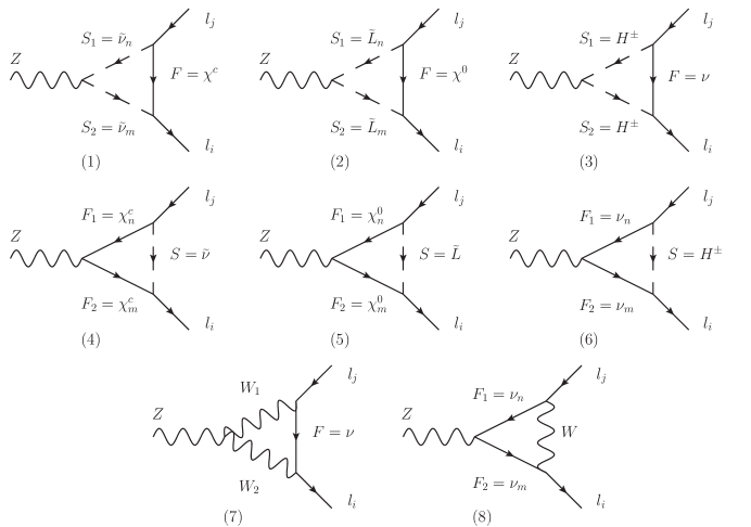
Figure 1: Feynman diagrams for the Z → l i ± l j ∓ → 𝑍 superscript subscript 𝑙 𝑖 plus-or-minus superscript subscript 𝑙 𝑗 minus-or-plus Z\rightarrow{{l_{i}}^{\pm}{l_{j}}^{\mp}} U ( 1 ) X 𝑈 subscript 1 𝑋 U(1)_{X}
The contributions obtained from Fig.1 1 F L , R ( A ) = F L , R α ( A ) ( α = 1 … 6 ) subscript 𝐹 𝐿 𝑅
𝐴 subscript superscript 𝐹 𝛼 𝐿 𝑅
𝐴 𝛼 1 … 6 F_{L,R}(A)=F^{\alpha}_{L,R}(A)(\alpha=1...6)
F L ( 1 , 2 , 3 ) ( A ) = i 2 H R S 2 F l ¯ i H Z S 1 S 2 ∗ H L S 1 ∗ l j F ¯ G 2 ( x F , x S 1 , x S 2 ) , subscript superscript 𝐹 1 2 3 𝐿 𝐴 𝑖 2 subscript superscript 𝐻 subscript 𝑆 2 𝐹 subscript ¯ 𝑙 𝑖 𝑅 superscript 𝐻 𝑍 subscript 𝑆 1 subscript superscript 𝑆 ∗ 2 subscript superscript 𝐻 subscript superscript 𝑆 ∗ 1 subscript 𝑙 𝑗 ¯ 𝐹 𝐿 subscript 𝐺 2 subscript 𝑥 𝐹 subscript 𝑥 subscript 𝑆 1 subscript 𝑥 subscript 𝑆 2 \displaystyle F^{(1,2,3)}_{L}(A)=\frac{i}{2}H^{S_{2}F\overline{l}_{i}}_{R}H^{Z{S_{1}}S^{\ast}_{2}}H^{S^{\ast}_{1}{l_{j}}\overline{F}}_{L}G_{2}(x_{F},x_{S_{1}},x_{S_{2}}),
F L ( 4 , 5 , 6 ) ( A ) = i 2 [ 2 m F 1 m F 2 m W 2 H R S F 2 l ¯ i H L Z F 1 F ¯ 2 H L S ∗ l j F ¯ 1 G 1 ( x S , x F 1 , x F 2 ) \displaystyle F^{(4,5,6)}_{L}(A)=\frac{i}{2}\Big{[}\frac{2m_{F_{1}}m_{F_{2}}}{m^{2}_{W}}H^{SF_{2}\overline{l}_{i}}_{R}H^{ZF_{1}\overline{F}_{2}}_{L}H^{S^{\ast}{l_{j}}\overline{F}_{1}}_{L}G_{1}(x_{S},x_{F_{1}},x_{F_{2}})
− H R S F 2 l ¯ i H R Z F 1 F ¯ 2 H L S ∗ l j F ¯ 1 G 2 ( x S , x F 1 , x F 2 ) ] , \displaystyle\hskip 45.52458pt-H^{SF_{2}\overline{l}_{i}}_{R}H^{ZF_{1}\overline{F}_{2}}_{R}H^{S^{\ast}{l_{j}}\overline{F}_{1}}_{L}G_{2}(x_{S},x_{F_{1}},x_{F_{2}})\Big{]},
F R α ( A ) = F L α ( A ) | L ↔ R , α = 1 … 6 . formulae-sequence subscript superscript 𝐹 𝛼 𝑅 𝐴 evaluated-at subscript superscript 𝐹 𝛼 𝐿 𝐴 ↔ 𝐿 𝑅 𝛼 1 … 6 \displaystyle F^{\alpha}_{R}(A)=F^{\alpha}_{L}(A)|_{L\leftrightarrow{R}},~{}~{}~{}\alpha=1...6. (40)
Here, x i = m i 2 / m W 2 subscript 𝑥 𝑖 superscript subscript 𝑚 𝑖 2 subscript superscript 𝑚 2 𝑊 x_{i}=m_{i}^{2}/m^{2}_{W} m i subscript 𝑚 𝑖 m_{i} m W subscript 𝑚 𝑊 m_{W} 1 S 1 subscript 𝑆 1 S_{1} S 2 subscript 𝑆 2 S_{2} H R S 2 F l ¯ i subscript superscript 𝐻 subscript 𝑆 2 𝐹 subscript ¯ 𝑙 𝑖 𝑅 H^{S_{2}F\overline{l}_{i}}_{R} ν ~ I ( R ) − χ ± − l ¯ i superscript ~ 𝜈 𝐼 𝑅 superscript 𝜒 plus-or-minus subscript ¯ 𝑙 𝑖 \tilde{\nu}^{I(R)}-\chi^{\pm}-\overline{l}_{i} H Z S 1 S 2 ∗ superscript 𝐻 𝑍 subscript 𝑆 1 subscript superscript 𝑆 ∗ 2 H^{Z{S_{1}}S^{\ast}_{2}} ν ~ R ( I ) − Z − ν ~ I ( R ) superscript ~ 𝜈 𝑅 𝐼 𝑍 superscript ~ 𝜈 𝐼 𝑅 \tilde{\nu}^{R(I)}-Z-\tilde{\nu}^{I(R)} H L S 1 ∗ l j F ¯ subscript superscript 𝐻 subscript superscript 𝑆 ∗ 1 subscript 𝑙 𝑗 ¯ 𝐹 𝐿 H^{S^{\ast}_{1}{l_{j}}\overline{F}}_{L} ν ~ R ( I ) − χ ¯ ± − l j superscript ~ 𝜈 𝑅 𝐼 superscript ¯ 𝜒 plus-or-minus subscript 𝑙 𝑗 \tilde{\nu}^{R(I)}-\overline{\chi}^{\pm}-l_{j} H R S 2 F l ¯ i subscript superscript 𝐻 subscript 𝑆 2 𝐹 subscript ¯ 𝑙 𝑖 𝑅 H^{S_{2}F\overline{l}_{i}}_{R} H Z S 1 S 2 ∗ superscript 𝐻 𝑍 subscript 𝑆 1 subscript superscript 𝑆 ∗ 2 H^{Z{S_{1}}S^{\ast}_{2}} H L S 1 ∗ l j F ¯ subscript superscript 𝐻 subscript superscript 𝑆 ∗ 1 subscript 𝑙 𝑗 ¯ 𝐹 𝐿 H^{S^{\ast}_{1}{l_{j}}\overline{F}}_{L} A 1 S 1 subscript 𝑆 1 S_{1} S 2 subscript 𝑆 2 S_{2} L ~ ~ 𝐿 \tilde{L} χ 0 superscript 𝜒 0 \chi^{0} H R L ~ n χ 0 l ¯ i , H Z L ~ m L ~ n ∗ subscript superscript 𝐻 subscript ~ 𝐿 𝑛 superscript 𝜒 0 subscript ¯ 𝑙 𝑖 𝑅 superscript 𝐻 𝑍 subscript ~ 𝐿 𝑚 superscript subscript ~ 𝐿 𝑛
H^{\tilde{L}_{n}\chi^{0}\overline{l}_{i}}_{R},~{}H^{Z{\tilde{L}_{m}}\tilde{L}_{n}^{*}} H L L ~ m ∗ l j χ ¯ 0 subscript superscript 𝐻 superscript subscript ~ 𝐿 𝑚 subscript 𝑙 𝑗 superscript ¯ 𝜒 0 𝐿 H^{\tilde{L}_{m}^{*}{l_{j}}\overline{\chi}^{0}}_{L} A 1 S 1 subscript 𝑆 1 S_{1} S 2 subscript 𝑆 2 S_{2} H ± superscript 𝐻 plus-or-minus H^{\pm} ν 𝜈 \nu H R H ± ν l ¯ i , H Z H ± H ± subscript superscript 𝐻 superscript 𝐻 plus-or-minus 𝜈 subscript ¯ 𝑙 𝑖 𝑅 superscript 𝐻 𝑍 superscript 𝐻 plus-or-minus superscript 𝐻 plus-or-minus
H^{H^{\pm}\nu\overline{l}_{i}}_{R},~{}H^{ZH^{\pm}H^{\pm}} H L H ± l j ν ¯ subscript superscript 𝐻 superscript 𝐻 plus-or-minus subscript 𝑙 𝑗 ¯ 𝜈 𝐿 H^{H^{\pm}{l_{j}}\overline{\nu}}_{L} A
For Fig.1 F 1 subscript 𝐹 1 F_{1} F 2 subscript 𝐹 2 F_{2} χ ± superscript 𝜒 plus-or-minus \chi^{\pm} S 𝑆 S ν ~ R ( I ) superscript ~ 𝜈 𝑅 𝐼 \tilde{\nu}^{R(I)} m F 1 subscript 𝑚 subscript 𝐹 1 m_{F_{1}} m F 2 subscript 𝑚 subscript 𝐹 2 m_{F_{2}} A 1 F 1 subscript 𝐹 1 F_{1} F 2 subscript 𝐹 2 F_{2} S 𝑆 S m F 1 subscript 𝑚 subscript 𝐹 1 m_{F_{1}} m F 2 subscript 𝑚 subscript 𝐹 2 m_{F_{2}} A 1 F 1 subscript 𝐹 1 F_{1} F 2 subscript 𝐹 2 F_{2} S 𝑆 S m F 1 subscript 𝑚 subscript 𝐹 1 m_{F_{1}} m F 2 subscript 𝑚 subscript 𝐹 2 m_{F_{2}} A
The specific form of the one-loop functions G i ( x 1 , x 2 , x 3 ) ( i = 1 … 3 ) subscript 𝐺 𝑖 subscript 𝑥 1 subscript 𝑥 2 subscript 𝑥 3 𝑖 1 … 3 G_{i}(x_{1},x_{2},x_{3})(i=1...3)
G 1 ( x 1 , x 2 , x 3 ) = 1 16 π 2 [ x 1 ln x 1 ( x 1 − x 2 ) ( x 1 − x 3 ) + x 2 ln x 2 ( x 2 − x 1 ) ( x 2 − x 3 ) + x 3 ln x 3 ( x 3 − x 1 ) ( x 3 − x 2 ) ] , subscript 𝐺 1 subscript 𝑥 1 subscript 𝑥 2 subscript 𝑥 3 1 16 superscript 𝜋 2 delimited-[] subscript 𝑥 1 subscript 𝑥 1 subscript 𝑥 1 subscript 𝑥 2 subscript 𝑥 1 subscript 𝑥 3 subscript 𝑥 2 subscript 𝑥 2 subscript 𝑥 2 subscript 𝑥 1 subscript 𝑥 2 subscript 𝑥 3 subscript 𝑥 3 subscript 𝑥 3 subscript 𝑥 3 subscript 𝑥 1 subscript 𝑥 3 subscript 𝑥 2 \displaystyle G_{1}(x_{1},x_{2},x_{3})\!=\!\frac{1}{16\pi^{2}}[\frac{x_{1}\ln{x_{1}}}{(x_{1}\!-\!x_{2})(x_{1}\!-\!x_{3})}+\frac{x_{2}\ln{x_{2}}}{(x_{2}\!-\!x_{1})(x_{2}\!-\!x_{3})}+\frac{x_{3}\ln{x_{3}}}{(x_{3}\!-\!x_{1})(x_{3}\!-\!x_{2})}],
G 2 ( x 1 , x 2 , x 3 ) = 1 16 π 2 [ x 1 2 ln x 1 ( x 1 − x 2 ) ( x 1 − x 3 ) + x 2 2 ln x 2 ( x 2 − x 1 ) ( x 2 − x 3 ) + x 3 2 ln x 3 ( x 3 − x 1 ) ( x 3 − x 2 ) ] . subscript 𝐺 2 subscript 𝑥 1 subscript 𝑥 2 subscript 𝑥 3 1 16 superscript 𝜋 2 delimited-[] superscript subscript 𝑥 1 2 subscript 𝑥 1 subscript 𝑥 1 subscript 𝑥 2 subscript 𝑥 1 subscript 𝑥 3 superscript subscript 𝑥 2 2 subscript 𝑥 2 subscript 𝑥 2 subscript 𝑥 1 subscript 𝑥 2 subscript 𝑥 3 superscript subscript 𝑥 3 2 subscript 𝑥 3 subscript 𝑥 3 subscript 𝑥 1 subscript 𝑥 3 subscript 𝑥 2 \displaystyle G_{2}(x_{1},x_{2},x_{3})\!=\!\frac{1}{16\pi^{2}}[\frac{x_{1}^{2}\ln{x_{1}}}{(x_{1}\!-\!x_{2})(x_{1}\!-\!x_{3})}+\frac{x_{2}^{2}\ln{x_{2}}}{(x_{2}\!-\!x_{1})(x_{2}\!-\!x_{3})}+\frac{x_{3}^{2}\ln{x_{3}}}{(x_{3}\!-\!x_{1})(x_{3}\!-\!x_{2})}]. (41)
The contributions obtained from Fig.1 1 F L , R ( W ) = F L , R α ( W ) ( α = 1 , 2 ) subscript 𝐹 𝐿 𝑅
𝑊 subscript superscript 𝐹 𝛼 𝐿 𝑅
𝑊 𝛼 1 2
F_{L,R}(W)=F^{\alpha}_{L,R}(W)(\alpha=1,2)
F L ( 1 , 2 ) ( W ) = i [ 3 H L W 2 F l ¯ i H Z W 1 W 2 ∗ H L W 1 ∗ l j F ¯ G 2 ( x F , x W 1 , x W 2 ) \displaystyle F^{(1,2)}_{L}(W)=i\Big{[}3H^{W_{2}F\overline{l}_{i}}_{L}H^{Z{W_{1}}W^{\ast}_{2}}H^{W^{\ast}_{1}{l_{j}}\overline{F}}_{L}G_{2}(x_{F},x_{W_{1}},x_{W_{2}})
− H L W F 2 l ¯ i H L Z F 1 F ¯ 2 H L F ¯ 1 l j W ∗ G 2 ( x W , x F 1 , x F 2 ) ] , \displaystyle\hskip 62.59596pt-H^{WF_{2}\overline{l}_{i}}_{L}H^{Z{F_{1}}\overline{F}_{2}}_{L}H^{\overline{F}_{1}{l_{j}}W^{\ast}}_{L}G_{2}(x_{W},x_{F_{1}},x_{F_{2}})\Big{]},
F R ( 1 , 2 ) ( W ) = 0 . subscript superscript 𝐹 1 2 𝑅 𝑊 0 \displaystyle F^{(1,2)}_{R}(W)=0. (42)
Here, F ( F 1 , F 2 ) 𝐹 subscript 𝐹 1 subscript 𝐹 2 F(F_{1},F_{2}) A A
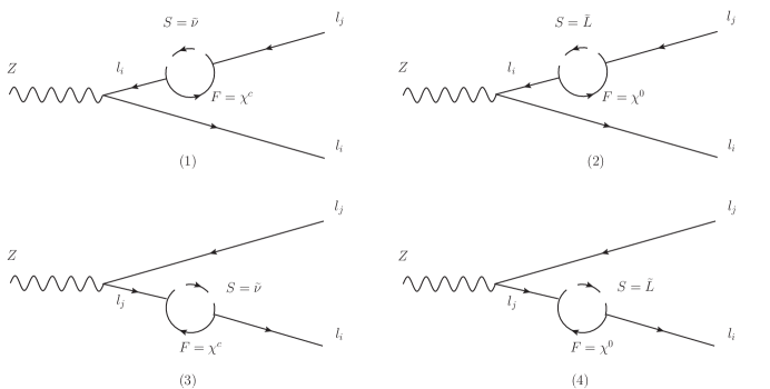
Figure 2: Feynman diagrams for the processes Z → l i ± l j ∓ → 𝑍 superscript subscript 𝑙 𝑖 plus-or-minus superscript subscript 𝑙 𝑗 minus-or-plus Z\rightarrow{{l_{i}}^{\pm}{l_{j}}^{\mp}} U ( 1 ) X 𝑈 subscript 1 𝑋 U(1)_{X} Z → l i ± l j ∓ → 𝑍 superscript subscript 𝑙 𝑖 plus-or-minus superscript subscript 𝑙 𝑗 minus-or-plus Z\rightarrow{{l_{i}}^{\pm}{l_{j}}^{\mp}}
The contributions obtained from Fig.2 F L , R ( B ) = F L , R α ( B ) ( α = 1 … 4 ) subscript 𝐹 𝐿 𝑅
𝐵 subscript superscript 𝐹 𝛼 𝐿 𝑅
𝐵 𝛼 1 … 4 F_{L,R}(B)=F^{\alpha}_{L,R}(B)(\alpha=1...4)
F L ( 1 , 2 ) ( B ) = H L Z l i l ¯ i m l j 2 − m l i 2 { I 1 ( x F , x S ) + m l j 2 m W 2 [ I 2 ( x F , x S ) − I 3 ( x F , x S ) ] \displaystyle F^{(1,2)}_{L}(B)=\frac{H^{Zl_{i}\overline{l}_{i}}_{L}}{m^{2}_{l_{j}}-m^{2}_{l_{i}}}\Big{\{}I_{1}(x_{F},x_{S})+\frac{m^{2}_{l_{j}}}{m^{2}_{W}}[I_{2}(x_{F},x_{S})-I_{3}(x_{F},x_{S})]
( m l j m F H R S F l ¯ i H R S ∗ l j F ¯ + m l i m F H L S F l ¯ i H L S ∗ l j F ¯ ) subscript 𝑚 subscript 𝑙 𝑗 subscript 𝑚 𝐹 subscript superscript 𝐻 𝑆 𝐹 subscript ¯ 𝑙 𝑖 𝑅 subscript superscript 𝐻 superscript 𝑆 ∗ subscript 𝑙 𝑗 ¯ 𝐹 𝑅 subscript 𝑚 subscript 𝑙 𝑖 subscript 𝑚 𝐹 subscript superscript 𝐻 𝑆 𝐹 subscript ¯ 𝑙 𝑖 𝐿 subscript superscript 𝐻 superscript 𝑆 ∗ subscript 𝑙 𝑗 ¯ 𝐹 𝐿 \displaystyle\hskip 62.59596pt(m_{l_{j}}m_{F}H^{SF\overline{l}_{i}}_{R}H^{S^{\ast}{l_{j}}\overline{F}}_{R}+m_{l_{i}}m_{F}H^{SF\overline{l}_{i}}_{L}H^{S^{\ast}{l_{j}}\overline{F}}_{L})
− 1 2 G 3 ( x F , x S ) ( m l j 2 H R S F l ¯ i H L S ∗ l j F ¯ + m l i m l j H L S F l ¯ i H R S ∗ l j F ¯ ) } , \displaystyle\hskip 62.59596pt-\frac{1}{2}G_{3}(x_{F},x_{S})(m^{2}_{l_{j}}H^{SF\overline{l}_{i}}_{R}H^{S^{\ast}{l_{j}}\overline{F}}_{L}+m_{l_{i}}m_{l_{j}}H^{SF\overline{l}_{i}}_{L}H^{S^{\ast}{l_{j}}\overline{F}}_{R})\Big{\}},
F L ( 3 , 4 ) ( B ) = H L Z l j l ¯ j m l i 2 − m l j 2 { I 1 ( x F , x S ) + m l i 2 m W 2 [ I 2 ( x F , x S ) − I 3 ( x F , x S ) ] \displaystyle F^{(3,4)}_{L}(B)=\frac{H^{Zl_{j}\overline{l}_{j}}_{L}}{m^{2}_{l_{i}}-m^{2}_{l_{j}}}\Big{\{}I_{1}(x_{F},x_{S})+\frac{m^{2}_{l_{i}}}{m^{2}_{W}}[I_{2}(x_{F},x_{S})-I_{3}(x_{F},x_{S})]
( m l i m F H R S F l ¯ i H R S ∗ l j F ¯ + m l j m F H L S F l ¯ i H L S ∗ l j F ¯ ) subscript 𝑚 subscript 𝑙 𝑖 subscript 𝑚 𝐹 subscript superscript 𝐻 𝑆 𝐹 subscript ¯ 𝑙 𝑖 𝑅 subscript superscript 𝐻 superscript 𝑆 ∗ subscript 𝑙 𝑗 ¯ 𝐹 𝑅 subscript 𝑚 subscript 𝑙 𝑗 subscript 𝑚 𝐹 subscript superscript 𝐻 𝑆 𝐹 subscript ¯ 𝑙 𝑖 𝐿 subscript superscript 𝐻 superscript 𝑆 ∗ subscript 𝑙 𝑗 ¯ 𝐹 𝐿 \displaystyle\hskip 62.59596pt(m_{l_{i}}m_{F}H^{SF\overline{l}_{i}}_{R}H^{S^{\ast}{l_{j}}\overline{F}}_{R}+m_{l_{j}}m_{F}H^{SF\overline{l}_{i}}_{L}H^{S^{\ast}{l_{j}}\overline{F}}_{L})
− 1 2 G 3 ( x F , x S ) ( m l i 2 H L S F l ¯ i H R S ∗ l j F ¯ + m l i m l j H R S F l ¯ i H L S ∗ l j F ¯ ) } , \displaystyle\hskip 62.59596pt-\frac{1}{2}G_{3}(x_{F},x_{S})(m^{2}_{l_{i}}H^{SF\overline{l}_{i}}_{L}H^{S^{\ast}{l_{j}}\overline{F}}_{R}+m_{l_{i}}m_{l_{j}}H^{SF\overline{l}_{i}}_{R}H^{S^{\ast}{l_{j}}\overline{F}}_{L})\Big{\}},
F R α ( B ) = F L α ( B ) | L ↔ R , α = 1 … 4 . formulae-sequence subscript superscript 𝐹 𝛼 𝑅 𝐵 evaluated-at subscript superscript 𝐹 𝛼 𝐿 𝐵 ↔ 𝐿 𝑅 𝛼 1 … 4 \displaystyle F^{\alpha}_{R}(B)=F^{\alpha}_{L}(B)|_{L\leftrightarrow{R}},~{}~{}~{}\alpha=1...4. (43)
H L Z l i l ¯ i = H L Z l j l ¯ j = i 2 ( − g 1 cos θ W ′ sin θ W + g 2 cos θ W cos θ W ′ + g Y X sin θ W ′ ) subscript superscript 𝐻 𝑍 subscript 𝑙 𝑖 subscript ¯ 𝑙 𝑖 𝐿 subscript superscript 𝐻 𝑍 subscript 𝑙 𝑗 subscript ¯ 𝑙 𝑗 𝐿 𝑖 2 subscript 𝑔 1 superscript subscript 𝜃 𝑊 ′ subscript 𝜃 𝑊 subscript 𝑔 2 subscript 𝜃 𝑊 superscript subscript 𝜃 𝑊 ′ subscript 𝑔 𝑌 𝑋 superscript subscript 𝜃 𝑊 ′ H^{Zl_{i}\overline{l}_{i}}_{L}=H^{Zl_{j}\overline{l}_{j}}_{L}=\frac{i}{2}(-g_{1}\cos\theta_{W}^{\prime}\sin\theta_{W}+g_{2}\cos\theta_{W}\cos\theta_{W}^{\prime}+g_{YX}\sin\theta_{W}^{\prime}) 2 F 𝐹 F S 𝑆 S m F subscript 𝑚 𝐹 m_{F} 2 F 𝐹 F S 𝑆 S m F subscript 𝑚 𝐹 m_{F} 2 2 1 1 2 2 2 2
Here
I 1 ( x 1 , x 2 ) = 1 16 π 2 [ 1 + log x 2 x 2 − x 1 + x 1 log x 1 − x 2 log x 2 ( x 2 − x 1 ) 2 ] , subscript 𝐼 1 subscript 𝑥 1 subscript 𝑥 2 1 16 superscript 𝜋 2 delimited-[] 1 subscript 𝑥 2 subscript 𝑥 2 subscript 𝑥 1 subscript 𝑥 1 subscript 𝑥 1 subscript 𝑥 2 subscript 𝑥 2 superscript subscript 𝑥 2 subscript 𝑥 1 2 \displaystyle I_{1}(x_{1},x_{2})=\frac{1}{16\pi^{2}}\Big{[}\frac{1+\log{x_{2}}}{x_{2}-x_{1}}+\frac{x_{1}\log{x_{1}}-x_{2}\log{x_{2}}}{(x_{2}-x_{1})^{2}}\Big{]},
I 2 ( x 1 , x 2 ) = 1 16 π 2 [ − 1 + log x 2 x 2 − x 1 − x 1 log x 1 − x 2 log x 2 ( x 2 − x 1 ) 2 ] , subscript 𝐼 2 subscript 𝑥 1 subscript 𝑥 2 1 16 superscript 𝜋 2 delimited-[] 1 subscript 𝑥 2 subscript 𝑥 2 subscript 𝑥 1 subscript 𝑥 1 subscript 𝑥 1 subscript 𝑥 2 subscript 𝑥 2 superscript subscript 𝑥 2 subscript 𝑥 1 2 \displaystyle I_{2}(x_{1},x_{2})=\frac{1}{16\pi^{2}}\Big{[}-\frac{1+\log{x_{2}}}{x_{2}-x_{1}}-\frac{x_{1}\log{x_{1}}-x_{2}\log{x_{2}}}{(x_{2}-x_{1})^{2}}\Big{]},
G 3 ( x 1 , x 2 ) = − 1 16 π 2 [ x 2 2 log x 2 − x 1 2 log x 1 ( x 2 − x 1 ) 2 + x 2 + 2 x 2 log x 2 ( x 1 − x 2 ) − 1 2 ] . subscript 𝐺 3 subscript 𝑥 1 subscript 𝑥 2 1 16 superscript 𝜋 2 delimited-[] subscript superscript 𝑥 2 2 subscript 𝑥 2 subscript superscript 𝑥 2 1 subscript 𝑥 1 superscript subscript 𝑥 2 subscript 𝑥 1 2 subscript 𝑥 2 2 subscript 𝑥 2 subscript 𝑥 2 subscript 𝑥 1 subscript 𝑥 2 1 2 \displaystyle G_{3}(x_{1},x_{2})=-\frac{1}{16\pi^{2}}\Big{[}\frac{x^{2}_{2}\log{x_{2}}-x^{2}_{1}\log{x_{1}}}{(x_{2}-x_{1})^{2}}+\frac{x_{2}+2x_{2}\log{x_{2}}}{(x_{1}-x_{2})}-\frac{1}{2}\Big{]}. (44)
Then, the branching ratios of Z → l i ± l j ∓ → 𝑍 superscript subscript 𝑙 𝑖 plus-or-minus superscript subscript 𝑙 𝑗 minus-or-plus Z\rightarrow{{l_{i}}^{\pm}{l_{j}}^{\mp}}
B r ( Z → l i ± l j ∓ ) = 1 12 π m Z Γ Z ( | F L Z | 2 + | F R Z | 2 ) 𝐵 𝑟 → 𝑍 superscript subscript 𝑙 𝑖 plus-or-minus superscript subscript 𝑙 𝑗 minus-or-plus 1 12 𝜋 subscript 𝑚 𝑍 subscript Γ 𝑍 superscript subscript superscript 𝐹 𝑍 𝐿 2 superscript subscript superscript 𝐹 𝑍 𝑅 2 \displaystyle Br(Z\rightarrow{{l_{i}}^{\pm}{l_{j}}^{\mp}})=\frac{1}{12\pi}\frac{m_{Z}}{\Gamma_{Z}}(|F^{Z}_{L}|^{2}+|F^{Z}_{R}|^{2})
= 1 12 π m Z Γ Z ( | F L ( A ) + F L ( W ) + F L ( B ) | 2 + | F R ( A ) + F R ( B ) | 2 ) , absent 1 12 𝜋 subscript 𝑚 𝑍 subscript Γ 𝑍 superscript subscript 𝐹 𝐿 𝐴 subscript 𝐹 𝐿 𝑊 subscript 𝐹 𝐿 𝐵 2 superscript subscript 𝐹 𝑅 𝐴 subscript 𝐹 𝑅 𝐵 2 \displaystyle\hskip 85.35826pt=\frac{1}{12\pi}\frac{m_{Z}}{\Gamma_{Z}}(|F_{L}(A)+F_{L}(W)+F_{L}(B)|^{2}+|F_{R}(A)+F_{R}(B)|^{2}), (45)
here Γ Z subscript Γ 𝑍 \Gamma_{Z} Γ Z ≃ 2.4952 similar-to-or-equals subscript Γ 𝑍 2.4952 \Gamma_{Z}\simeq 2.4952 IN4
IV Higgs boson decays h → l i ± l j ∓ → ℎ superscript subscript 𝑙 𝑖 plus-or-minus superscript subscript 𝑙 𝑗 minus-or-plus h\rightarrow{{l_{i}}^{\pm}{l_{j}}^{\mp}}
In this section, we analyze the LFV processes h → l i ± l j ∓ → ℎ superscript subscript 𝑙 𝑖 plus-or-minus superscript subscript 𝑙 𝑗 minus-or-plus h\rightarrow{{l_{i}}^{\pm}{l_{j}}^{\mp}} 3 4
The corresponding effective amplitude can be written as
ℳ = l ¯ i ( F L P L + F R P R ) l j h , ℳ subscript ¯ 𝑙 𝑖 subscript 𝐹 𝐿 subscript 𝑃 𝐿 subscript 𝐹 𝑅 subscript 𝑃 𝑅 subscript 𝑙 𝑗 ℎ \displaystyle\mathcal{M}=\overline{l}_{i}(F_{L}P_{L}+F_{R}P_{R}){l_{j}}h, (46)
with
F L , R h = F L , R ( C ) + F L , R ( D ) , subscript superscript 𝐹 ℎ 𝐿 𝑅
subscript 𝐹 𝐿 𝑅
𝐶 subscript 𝐹 𝐿 𝑅
𝐷 \displaystyle F^{h}_{L,R}=F_{L,R}(C)+F_{L,R}(D), (47)
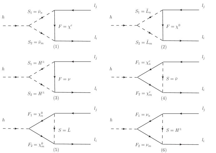
Figure 3: Feynman diagrams for the processes h → l i ± l j ∓ → ℎ superscript subscript 𝑙 𝑖 plus-or-minus superscript subscript 𝑙 𝑗 minus-or-plus h\rightarrow{{l_{i}}^{\pm}{l_{j}}^{\mp}} U ( 1 ) X 𝑈 subscript 1 𝑋 U(1)_{X} h → l i ± l j ∓ → ℎ superscript subscript 𝑙 𝑖 plus-or-minus superscript subscript 𝑙 𝑗 minus-or-plus h\rightarrow{{l_{i}}^{\pm}{l_{j}}^{\mp}}
The contribution obtained by Fig.3 F L , R ( C ) = F L , R α ( C ) ( α = 1 … 6 ) subscript 𝐹 𝐿 𝑅
𝐶 subscript superscript 𝐹 𝛼 𝐿 𝑅
𝐶 𝛼 1 … 6 F_{L,R}(C)=F^{\alpha}_{L,R}(C)(\alpha=1...6)
F L ( 1 , 2 , 3 ) ( C ) = m F m N p 2 H h S 1 S 2 ∗ H L S 2 F l ¯ i H L S 1 ∗ l j F ¯ G 1 ( x F , x S 1 , x S 2 ) , subscript superscript 𝐹 1 2 3 𝐿 𝐶 subscript 𝑚 𝐹 subscript superscript 𝑚 2 subscript 𝑁 𝑝 superscript 𝐻 ℎ subscript 𝑆 1 subscript superscript 𝑆 ∗ 2 subscript superscript 𝐻 subscript 𝑆 2 𝐹 subscript ¯ 𝑙 𝑖 𝐿 subscript superscript 𝐻 subscript superscript 𝑆 ∗ 1 subscript 𝑙 𝑗 ¯ 𝐹 𝐿 subscript 𝐺 1 subscript 𝑥 𝐹 subscript 𝑥 subscript 𝑆 1 subscript 𝑥 subscript 𝑆 2 \displaystyle F^{(1,2,3)}_{L}(C)=\frac{m_{F}}{m^{2}_{N_{p}}}H^{h{S_{1}}S^{\ast}_{2}}H^{S_{2}F\overline{l}_{i}}_{L}H^{S^{\ast}_{1}{l_{j}}\overline{F}}_{L}G_{1}(x_{F},x_{S_{1}},x_{S_{2}}),
F L ( 4 , 5 , 6 ) ( C ) = m F 1 m F 2 m N p 2 H L S F 2 l ¯ i H L h F 1 F ¯ 2 H L S ∗ l j F ¯ 1 G 1 ( x S , x F 1 , x F 2 ) subscript superscript 𝐹 4 5 6 𝐿 𝐶 subscript 𝑚 subscript 𝐹 1 subscript 𝑚 subscript 𝐹 2 subscript superscript 𝑚 2 subscript 𝑁 𝑝 subscript superscript 𝐻 𝑆 subscript 𝐹 2 subscript ¯ 𝑙 𝑖 𝐿 subscript superscript 𝐻 ℎ subscript 𝐹 1 subscript ¯ 𝐹 2 𝐿 subscript superscript 𝐻 superscript 𝑆 ∗ subscript 𝑙 𝑗 subscript ¯ 𝐹 1 𝐿 subscript 𝐺 1 subscript 𝑥 𝑆 subscript 𝑥 subscript 𝐹 1 subscript 𝑥 subscript 𝐹 2 \displaystyle F^{(4,5,6)}_{L}(C)=\frac{m_{F_{1}}m_{F_{2}}}{m^{2}_{N_{p}}}H^{SF_{2}\overline{l}_{i}}_{L}H^{h{F_{1}}\overline{F}_{2}}_{L}H^{S^{\ast}{l_{j}}\overline{F}_{1}}_{L}G_{1}(x_{S},x_{F_{1}},x_{F_{2}})
+ H L S F 2 l ¯ i H R h F 1 F ¯ 2 H L S ∗ l j F ¯ 1 G 2 ( x S , x F 1 , x F 2 ) , subscript superscript 𝐻 𝑆 subscript 𝐹 2 subscript ¯ 𝑙 𝑖 𝐿 subscript superscript 𝐻 ℎ subscript 𝐹 1 subscript ¯ 𝐹 2 𝑅 subscript superscript 𝐻 superscript 𝑆 ∗ subscript 𝑙 𝑗 subscript ¯ 𝐹 1 𝐿 subscript 𝐺 2 subscript 𝑥 𝑆 subscript 𝑥 subscript 𝐹 1 subscript 𝑥 subscript 𝐹 2 \displaystyle\hskip 68.28644pt+H^{SF_{2}\overline{l}_{i}}_{L}H^{h{F_{1}}\overline{F}_{2}}_{R}H^{S^{\ast}{l_{j}}\overline{F}_{1}}_{L}G_{2}(x_{S},x_{F_{1}},x_{F_{2}}),
F R α ( C ) = F L α ( C ) | L ↔ R , α = 1 … 6 . formulae-sequence subscript superscript 𝐹 𝛼 𝑅 𝐶 evaluated-at subscript superscript 𝐹 𝛼 𝐿 𝐶 ↔ 𝐿 𝑅 𝛼 1 … 6 \displaystyle F^{\alpha}_{R}(C)=F^{\alpha}_{L}(C)|_{L\leftrightarrow{R}},~{}~{}~{}\alpha=1...6. (48)
The Figs.3 3 3 1 1 1 3 H h S 1 S 2 ∗ → H h ν ~ R ν ~ R ∗ ( H h ν ~ I ν ~ I ∗ ) → superscript 𝐻 ℎ subscript 𝑆 1 subscript superscript 𝑆 ∗ 2 superscript 𝐻 ℎ superscript ~ 𝜈 𝑅 superscript ~ 𝜈 𝑅
superscript 𝐻 ℎ superscript ~ 𝜈 𝐼 superscript ~ 𝜈 𝐼
H^{h{S_{1}}S^{\ast}_{2}}\rightarrow H^{h\tilde{\nu}^{R}\tilde{\nu}^{R*}}(H^{h\tilde{\nu}^{I}\tilde{\nu}^{I*}}) H h ν ~ R ν ~ R ∗ superscript 𝐻 ℎ superscript ~ 𝜈 𝑅 superscript ~ 𝜈 𝑅
H^{h\tilde{\nu}^{R}\tilde{\nu}^{R*}} UU3 H h ν ~ I ν ~ I ∗ superscript 𝐻 ℎ superscript ~ 𝜈 𝐼 superscript ~ 𝜈 𝐼
H^{h\tilde{\nu}^{I}\tilde{\nu}^{I*}} H h ν ~ R ν ~ R ∗ superscript 𝐻 ℎ superscript ~ 𝜈 𝑅 superscript ~ 𝜈 𝑅
H^{h\tilde{\nu}^{R}\tilde{\nu}^{R*}} Z R → Z I → superscript 𝑍 𝑅 superscript 𝑍 𝐼 Z^{R}\rightarrow Z^{I}
For Fig.3 S 1 subscript 𝑆 1 S_{1} S 2 subscript 𝑆 2 S_{2} H h S 1 S 2 ∗ → H h L ~ L ~ ∗ → superscript 𝐻 ℎ subscript 𝑆 1 subscript superscript 𝑆 ∗ 2 superscript 𝐻 ℎ ~ 𝐿 superscript ~ 𝐿 H^{h{S_{1}}S^{\ast}_{2}}\rightarrow H^{h\tilde{L}\tilde{L}^{*}}
H h L ~ n L ~ m ∗ = i 4 { ∑ a = 1 3 Z m , a E , ∗ Z n , a E ( ( g 2 2 − g Y X g X − g 1 2 − g Y X 2 ) ( v d Z b 1 H − v u Z b 2 H ) + g Y X g X ( v η ¯ Z b 4 H \displaystyle H^{h\tilde{L}_{n}\tilde{L}^{*}_{m}}=\frac{i}{4}\Big{\{}\sum_{a=1}^{3}Z_{m,a}^{E,*}Z_{n,a}^{E}\Big{(}(g_{2}^{2}-g_{YX}g_{X}-g_{1}^{2}-g_{YX}^{2})(v_{d}Z_{b1}^{H}-v_{u}Z_{b2}^{H})+g_{YX}g_{X}(v_{\overline{\eta}}Z_{b4}^{H}
− v η Z b 3 H ) ) + ∑ a = 1 3 Z m , 3 + a E , ∗ Z n , 3 + a E ( ( 2 g 1 2 + 2 g Y X 2 + 3 g Y X g X + g X 2 ) ( v d Z b 1 H − v u Z b 2 H ) \displaystyle\hskip 45.52458pt-v_{\eta}Z_{b3}^{H})\Big{)}+\sum_{a=1}^{3}Z_{m,3+a}^{E,*}Z_{n,3+a}^{E}\Big{(}(2g_{1}^{2}+2g_{YX}^{2}+3g_{YX}g_{X}+g_{X}^{2})(v_{d}Z_{b1}^{H}-v_{u}Z_{b2}^{H})
+ 2 ( g Y X g X + g X 2 ) ( − v η ¯ Z b 4 H + v η Z b 3 H ) ) + ( ∑ a = 1 3 Z m , a E , ∗ Z n , 3 + a E + ∑ a = 1 3 Z m , 3 + a E , ∗ Z n , a E ) \displaystyle\hskip 45.52458pt+2(g_{YX}g_{X}+g_{X}^{2})(-v_{\overline{\eta}}Z_{b4}^{H}+v_{\eta}Z_{b3}^{H})\Big{)}+\Big{(}\sum_{a=1}^{3}Z_{m,a}^{E,*}Z_{n,3+a}^{E}+\sum_{a=1}^{3}Z_{m,3+a}^{E,*}Z_{n,a}^{E}\Big{)}
× [ − 2 2 T e , a Z b 1 H + Y e , a ( 2 ( v S λ H + 2 μ ) Z b 2 H + 2 v u λ H Z b 5 H ) ] } . \displaystyle\hskip 45.52458pt\times\Big{[}-2\sqrt{2}T_{e,a}Z_{b1}^{H}+Y_{e,a}\Big{(}2(v_{S}\lambda_{H}+\sqrt{2}{\mu})Z_{b2}^{H}+2v_{u}\lambda_{H}Z_{b5}^{H}\Big{)}\Big{]}\Big{\}}. (49)
For Fig.3
H h S 1 S 2 ∗ → H h H m ± H n ± ∗ → superscript 𝐻 ℎ subscript 𝑆 1 subscript superscript 𝑆 ∗ 2 superscript 𝐻 ℎ subscript superscript 𝐻 plus-or-minus 𝑚 subscript superscript 𝐻 plus-or-minus absent 𝑛 \displaystyle H^{h{S_{1}}S^{\ast}_{2}}\rightarrow H^{hH^{\pm}_{m}H^{\pm*}_{n}}
= i 4 { ( − Z b 2 H Z m 2 + − Z b 1 H Z m 1 + ) ( [ ( g Y X + g X ) 2 + g 1 2 + g 2 2 ] ( v u Z n 2 + + v d Z n 1 + ) + ( g 2 2 − 2 λ H 2 ) \displaystyle=\frac{i}{4}\Big{\{}(-Z_{b2}^{H}Z_{m2}^{+}-Z_{b1}^{H}Z_{m1}^{+})\Big{(}[(g_{YX}+g_{X})^{2}+g_{1}^{2}+g_{2}^{2}](v_{u}Z_{n2}^{+}+v_{d}Z_{n1}^{+})+(g_{2}^{2}-2\lambda_{H}^{2})
× ( v d Z n 1 + − v u Z n 2 + ) ) + ( Z b 2 H Z m 1 + + Z b 1 H Z m 2 + ) ( [ ( g Y X + g X ) 2 − 2 g 2 2 + g 1 2 + 2 λ H 2 ] ( v u Z n 1 + \displaystyle\times(v_{d}Z_{n1}^{+}-v_{u}Z_{n2}^{+})\Big{)}+(Z_{b2}^{H}Z_{m1}^{+}+Z_{b1}^{H}Z_{m2}^{+})\Big{(}[(g_{YX}+g_{X})^{2}-2g_{2}^{2}+g_{1}^{2}+2\lambda_{H}^{2}](v_{u}Z_{n1}^{+}
+ v d Z n 2 + ) ) − 2 Z b 4 H ( Z m 2 + − Z m 1 + ) ( ( g Y X g X + g X 2 ) v η ¯ ( Z n 2 + + Z n 1 + ) + λ c v η λ H ( Z n 1 + − Z n 2 + ) ) \displaystyle+v_{d}Z_{n2}^{+})\Big{)}-2Z_{b4}^{H}(Z_{m2}^{+}-Z_{m1}^{+})\Big{(}(g_{YX}g_{X}+g_{X}^{2})v_{\overline{\eta}}(Z_{n2}^{+}+Z_{n1}^{+})+\lambda_{c}v_{\eta}\lambda_{H}(Z_{n1}^{+}-Z_{n2}^{+})\Big{)}
+ Z b 3 H ( Z m 2 + + Z m 1 + ) ( ( g Y X g X + g X 2 ) ( v η Z n 1 + − v η Z n 2 + ) + λ c v η ¯ λ H ∗ ( Z n 1 + + Z n 2 + ) ) superscript subscript 𝑍 𝑏 3 𝐻 superscript subscript 𝑍 𝑚 2 superscript subscript 𝑍 𝑚 1 subscript 𝑔 𝑌 𝑋 subscript 𝑔 𝑋 superscript subscript 𝑔 𝑋 2 subscript 𝑣 𝜂 superscript subscript 𝑍 𝑛 1 subscript 𝑣 𝜂 superscript subscript 𝑍 𝑛 2 subscript 𝜆 𝑐 subscript 𝑣 ¯ 𝜂 superscript subscript 𝜆 𝐻 superscript subscript 𝑍 𝑛 1 superscript subscript 𝑍 𝑛 2 \displaystyle+Z_{b3}^{H}(Z_{m2}^{+}+Z_{m1}^{+})\Big{(}(g_{YX}g_{X}+g_{X}^{2})(v_{\eta}Z_{n1}^{+}-v_{\eta}Z_{n2}^{+})+\lambda_{c}v_{\overline{\eta}}\lambda_{H}^{*}(Z_{n1}^{+}+Z_{n2}^{+})\Big{)}
+ Z b 5 H ( Z m 2 + + Z m 1 + ) ( Z n 2 + + Z n 1 + ) ( 2 T λ , H + 2 λ H ( κ v s + 2 M S + 2 μ + λ H v S ) ) } . \displaystyle+Z_{b5}^{H}(Z_{m2}^{+}+Z_{m1}^{+})(Z_{n2}^{+}+Z_{n1}^{+})\Big{(}\sqrt{2}T_{{\lambda},H}+2\lambda_{H}(\kappa v_{s}+\sqrt{2}M_{S}+\sqrt{2}{\mu}+\lambda_{H}v_{S})\Big{)}\Big{\}}. (50)
For Fig.3 F 1 ( F 2 ) subscript 𝐹 1 subscript 𝐹 2 F_{1}(F_{2}) m F 1 ( m F 2 ) subscript 𝑚 subscript 𝐹 1 subscript 𝑚 subscript 𝐹 2 m_{F_{1}}(m_{F_{2}})
H L h F 1 F ¯ 2 → H L h χ n ± χ ¯ m ± = − i 2 ( g 2 U m 1 ∗ V n 2 ∗ Z b 2 H + U m 2 ∗ ( g 2 V n 1 ∗ Z b 1 H + λ H V n 2 ∗ Z b 5 H ) ) , → subscript superscript 𝐻 ℎ subscript 𝐹 1 subscript ¯ 𝐹 2 𝐿 subscript superscript 𝐻 ℎ subscript superscript 𝜒 plus-or-minus 𝑛 subscript superscript ¯ 𝜒 plus-or-minus 𝑚 𝐿 𝑖 2 subscript 𝑔 2 superscript subscript 𝑈 𝑚 1 superscript subscript 𝑉 𝑛 2 superscript subscript 𝑍 𝑏 2 𝐻 superscript subscript 𝑈 𝑚 2 subscript 𝑔 2 superscript subscript 𝑉 𝑛 1 superscript subscript 𝑍 𝑏 1 𝐻 subscript 𝜆 𝐻 superscript subscript 𝑉 𝑛 2 superscript subscript 𝑍 𝑏 5 𝐻 \displaystyle H^{h{F_{1}}\overline{F}_{2}}_{L}\rightarrow H^{h\chi^{\pm}_{n}\overline{\chi}^{\pm}_{m}}_{L}=-\frac{i}{\sqrt{2}}\Big{(}g_{2}U_{m1}^{*}V_{n2}^{*}Z_{b2}^{H}+U_{m2}^{*}(g_{2}V_{n1}^{*}Z_{b1}^{H}+\lambda_{H}V_{n2}^{*}Z_{b5}^{H})\Big{)},
H R h F 1 F ¯ 2 → H R h χ n ± χ ¯ m ± = − i 2 ( g 2 U n 1 V m 2 Z b 2 H + U n 2 ( g 2 V m 1 Z b 1 H + λ H ∗ V m 2 Z b 5 H ) ) . → subscript superscript 𝐻 ℎ subscript 𝐹 1 subscript ¯ 𝐹 2 𝑅 subscript superscript 𝐻 ℎ subscript superscript 𝜒 plus-or-minus 𝑛 subscript superscript ¯ 𝜒 plus-or-minus 𝑚 𝑅 𝑖 2 subscript 𝑔 2 subscript 𝑈 𝑛 1 subscript 𝑉 𝑚 2 superscript subscript 𝑍 𝑏 2 𝐻 subscript 𝑈 𝑛 2 subscript 𝑔 2 subscript 𝑉 𝑚 1 superscript subscript 𝑍 𝑏 1 𝐻 superscript subscript 𝜆 𝐻 subscript 𝑉 𝑚 2 superscript subscript 𝑍 𝑏 5 𝐻 \displaystyle H^{h{F_{1}}\overline{F}_{2}}_{R}\rightarrow H^{h\chi^{\pm}_{n}\overline{\chi}^{\pm}_{m}}_{R}=-\frac{i}{\sqrt{2}}\Big{(}g_{2}U_{n1}V_{m2}Z_{b2}^{H}+U_{n2}(g_{2}V_{m1}Z_{b1}^{H}+\lambda_{H}^{*}V_{m2}Z_{b5}^{H})\Big{)}. (51)
For Fig.3 F 1 ( F 2 ) subscript 𝐹 1 subscript 𝐹 2 F_{1}(F_{2}) m F 1 ( m F 2 ) subscript 𝑚 subscript 𝐹 1 subscript 𝑚 subscript 𝐹 2 m_{F_{1}}(m_{F_{2}}) H h χ 0 χ ¯ 0 superscript 𝐻 ℎ superscript 𝜒 0 superscript ¯ 𝜒 0 H^{h\chi^{0}\overline{\chi}^{0}} UU5 3 F 1 subscript 𝐹 1 F_{1} F 2 subscript 𝐹 2 F_{2} ( m F 1 , m F 2 ) subscript 𝑚 subscript 𝐹 1 subscript 𝑚 subscript 𝐹 2 (m_{F_{1}},m_{F_{2}}) 3
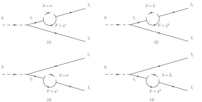
Figure 4: Feynman diagrams for the processes h → l i ± l j ∓ → ℎ superscript subscript 𝑙 𝑖 plus-or-minus superscript subscript 𝑙 𝑗 minus-or-plus h\rightarrow{{l_{i}}^{\pm}{l_{j}}^{\mp}} U ( 1 ) X 𝑈 subscript 1 𝑋 U(1)_{X} h → l i ± l j ∓ → ℎ superscript subscript 𝑙 𝑖 plus-or-minus superscript subscript 𝑙 𝑗 minus-or-plus h\rightarrow{{l_{i}}^{\pm}{l_{j}}^{\mp}}
The contributions obtained from Fig.4 F L , R ( D ) = F L , R α ( D ) ( α = 1 … 4 ) subscript 𝐹 𝐿 𝑅
𝐷 subscript superscript 𝐹 𝛼 𝐿 𝑅
𝐷 𝛼 1 … 4 F_{L,R}(D)=F^{\alpha}_{L,R}(D)(\alpha=1...4)
F L ( 1 , 2 ) ( D ) = H L h l i l ¯ i m l j 2 − m l i 2 { I 1 ( x F , x S ) + m l j 2 m W 2 [ I 2 ( x F , x S ) − I 3 ( x F , x S ) ] \displaystyle F^{(1,2)}_{L}(D)=\frac{H^{hl_{i}\overline{l}_{i}}_{L}}{m^{2}_{l_{j}}-m^{2}_{l_{i}}}\Big{\{}I_{1}(x_{F},x_{S})+\frac{m^{2}_{l_{j}}}{m^{2}_{W}}[I_{2}(x_{F},x_{S})-I_{3}(x_{F},x_{S})]
( m l j m F H R S F l ¯ i H R S ∗ l j F ¯ + m l i m F H L S F l ¯ i H L S ∗ l j F ¯ ) subscript 𝑚 subscript 𝑙 𝑗 subscript 𝑚 𝐹 subscript superscript 𝐻 𝑆 𝐹 subscript ¯ 𝑙 𝑖 𝑅 subscript superscript 𝐻 superscript 𝑆 ∗ subscript 𝑙 𝑗 ¯ 𝐹 𝑅 subscript 𝑚 subscript 𝑙 𝑖 subscript 𝑚 𝐹 subscript superscript 𝐻 𝑆 𝐹 subscript ¯ 𝑙 𝑖 𝐿 subscript superscript 𝐻 superscript 𝑆 ∗ subscript 𝑙 𝑗 ¯ 𝐹 𝐿 \displaystyle\hskip 62.59596pt(m_{l_{j}}m_{F}H^{SF\overline{l}_{i}}_{R}H^{S^{\ast}{l_{j}}\overline{F}}_{R}+m_{l_{i}}m_{F}H^{SF\overline{l}_{i}}_{L}H^{S^{\ast}{l_{j}}\overline{F}}_{L})
− 1 2 G 3 ( x F , x S ) ( m l j 2 H R S F l ¯ i H L S ∗ l j F ¯ + m l i m l j H L S F l ¯ i H R S ∗ l j F ¯ ) } , \displaystyle\hskip 62.59596pt-\frac{1}{2}G_{3}(x_{F},x_{S})(m^{2}_{l_{j}}H^{SF\overline{l}_{i}}_{R}H^{S^{\ast}{l_{j}}\overline{F}}_{L}+m_{l_{i}}m_{l_{j}}H^{SF\overline{l}_{i}}_{L}H^{S^{\ast}{l_{j}}\overline{F}}_{R})\Big{\}},
F L ( 3 , 4 ) ( D ) = H L h l j l ¯ j m l i 2 − m l j 2 { I 1 ( x F , x S ) + m l i 2 m W 2 [ I 2 ( x F , x S ) − I 3 ( x F , x S ) ] \displaystyle F^{(3,4)}_{L}(D)=\frac{H^{hl_{j}\overline{l}_{j}}_{L}}{m^{2}_{l_{i}}-m^{2}_{l_{j}}}\Big{\{}I_{1}(x_{F},x_{S})+\frac{m^{2}_{l_{i}}}{m^{2}_{W}}[I_{2}(x_{F},x_{S})-I_{3}(x_{F},x_{S})]
( m l i m F H R S F l ¯ i H R S ∗ l j F ¯ + m l j m F H L S F l ¯ i H L S ∗ l j F ¯ ) subscript 𝑚 subscript 𝑙 𝑖 subscript 𝑚 𝐹 subscript superscript 𝐻 𝑆 𝐹 subscript ¯ 𝑙 𝑖 𝑅 subscript superscript 𝐻 superscript 𝑆 ∗ subscript 𝑙 𝑗 ¯ 𝐹 𝑅 subscript 𝑚 subscript 𝑙 𝑗 subscript 𝑚 𝐹 subscript superscript 𝐻 𝑆 𝐹 subscript ¯ 𝑙 𝑖 𝐿 subscript superscript 𝐻 superscript 𝑆 ∗ subscript 𝑙 𝑗 ¯ 𝐹 𝐿 \displaystyle\hskip 62.59596pt(m_{l_{i}}m_{F}H^{SF\overline{l}_{i}}_{R}H^{S^{\ast}{l_{j}}\overline{F}}_{R}+m_{l_{j}}m_{F}H^{SF\overline{l}_{i}}_{L}H^{S^{\ast}{l_{j}}\overline{F}}_{L})
− 1 2 G 3 ( x F , x S ) ( m l i 2 H L S F l ¯ i H R S ∗ l j F ¯ + m l i m l j H R S F l ¯ i H L S ∗ l j F ¯ ) } , \displaystyle\hskip 62.59596pt-\frac{1}{2}G_{3}(x_{F},x_{S})(m^{2}_{l_{i}}H^{SF\overline{l}_{i}}_{L}H^{S^{\ast}{l_{j}}\overline{F}}_{R}+m_{l_{i}}m_{l_{j}}H^{SF\overline{l}_{i}}_{R}H^{S^{\ast}{l_{j}}\overline{F}}_{L})\Big{\}},
F R α ( D ) = F L α ( D ) | L ↔ R , α = 1 … 4 . formulae-sequence subscript superscript 𝐹 𝛼 𝑅 𝐷 evaluated-at subscript superscript 𝐹 𝛼 𝐿 𝐷 ↔ 𝐿 𝑅 𝛼 1 … 4 \displaystyle F^{\alpha}_{R}(D)=F^{\alpha}_{L}(D)|_{L\leftrightarrow{R}},~{}~{}~{}\alpha=1...4. (52)
The lepton-h-lepton coupling is denoted by H L h l i l ¯ i = − i 2 Y e , i Z b 1 H superscript subscript 𝐻 𝐿 ℎ subscript 𝑙 𝑖 subscript ¯ 𝑙 𝑖 𝑖 2 subscript 𝑌 𝑒 𝑖
superscript subscript 𝑍 𝑏 1 𝐻 H_{L}^{hl_{i}\overline{l}_{i}}=-\frac{i}{\sqrt{2}}Y_{e,i}Z_{b1}^{H} 4 m F subscript 𝑚 𝐹 m_{F} 2
Then, the branching ratio of h → l i ± l j ∓ → ℎ superscript subscript 𝑙 𝑖 plus-or-minus superscript subscript 𝑙 𝑗 minus-or-plus h\rightarrow{{l_{i}}^{\pm}{l_{j}}^{\mp}}
B r ( h → l i ± l j ∓ ) = 1 16 π m h Γ h ( | F L h | 2 + | F R h | 2 ) , 𝐵 𝑟 → ℎ superscript subscript 𝑙 𝑖 plus-or-minus superscript subscript 𝑙 𝑗 minus-or-plus 1 16 𝜋 subscript 𝑚 ℎ subscript Γ ℎ superscript subscript superscript 𝐹 ℎ 𝐿 2 superscript subscript superscript 𝐹 ℎ 𝑅 2 \displaystyle Br(h\rightarrow{{l_{i}}^{\pm}{l_{j}}^{\mp}})=\frac{1}{16\pi}\frac{m_{h}}{\Gamma_{h}}(|F^{h}_{L}|^{2}+|F^{h}_{R}|^{2}), (53)
here Γ h ≃ Γ h S M ≃ 4.1 × 10 − 3 similar-to-or-equals subscript Γ ℎ subscript superscript Γ 𝑆 𝑀 ℎ similar-to-or-equals 4.1 superscript 10 3 \Gamma_{h}\simeq\Gamma^{SM}_{h}\simeq 4.1\times 10^{-3} Z184 Γ h subscript Γ ℎ \Gamma_{h} U ( 1 ) X 𝑈 subscript 1 𝑋 U(1)_{X} Γ h S M subscript superscript Γ 𝑆 𝑀 ℎ \Gamma^{SM}_{h} U ( 1 ) X 𝑈 subscript 1 𝑋 U(1)_{X} Γ h subscript Γ ℎ \Gamma_{h} Γ h S M subscript superscript Γ 𝑆 𝑀 ℎ \Gamma^{SM}_{h}
V Numerical analysis
In this section, we study the numerical results and consider the experiments constraints from the lightest CP-even Higgs mass m h 0 subscript 𝑚 superscript ℎ 0 m_{h^{0}} IN2 ; IN3 ; xin1 ; ZPG1 ; ZPG2 ; TanBP l j → l i γ → subscript 𝑙 𝑗 subscript 𝑙 𝑖 𝛾 l_{j}\rightarrow{l_{i}\gamma} μ → e γ → 𝜇 𝑒 𝛾 \mu\rightarrow{e\gamma} μ → e γ → 𝜇 𝑒 𝛾 \mu\rightarrow{e\gamma} T1 Z → e μ → 𝑍 𝑒 𝜇 Z\rightarrow e\mu Z → e τ → 𝑍 𝑒 𝜏 Z\rightarrow e\tau Z → μ τ → 𝑍 𝜇 𝜏 Z\rightarrow\mu\tau h → e μ → ℎ 𝑒 𝜇 h\rightarrow e\mu h → e τ → ℎ 𝑒 𝜏 h\rightarrow e\tau h → μ τ → ℎ 𝜇 𝜏 h\rightarrow\mu\tau
According to the latest LHC dataw1 ; w2 ; w3 ; w4 ; w5 ; w6 700 GeV 700 GeV 700~{}{\rm GeV} 1100 GeV 1100 GeV 1100~{}{\rm GeV} 1500 GeV 1500 GeV 1500~{}{\rm GeV} M Z ′ > 5.1 subscript 𝑀 superscript 𝑍 ′ 5.1 M_{Z^{\prime}}>5.1 Z ′ superscript 𝑍 ′ Z^{\prime} xin1 Z ′ superscript 𝑍 ′ Z^{\prime} M Z ′ / g X ≥ 6 subscript 𝑀 superscript 𝑍 ′ subscript 𝑔 𝑋 6 M_{Z^{\prime}}/g_{X}\geq 6 ZPG1 ; ZPG2 tan β η < 1.5 subscript 𝛽 𝜂 1.5 \tan\beta_{\eta}<1.5 TanBP
g X = 0.3 , g Y X = 0.1 , λ H = 0.1 , λ C = − 0.2 , v η 2 + v η ¯ 2 = 17 TeV , formulae-sequence subscript 𝑔 𝑋 0.3 formulae-sequence subscript 𝑔 𝑌 𝑋 0.1 formulae-sequence subscript 𝜆 𝐻 0.1 formulae-sequence subscript 𝜆 𝐶 0.2 superscript subscript 𝑣 𝜂 2 superscript subscript 𝑣 ¯ 𝜂 2 17 TeV \displaystyle g_{X}=0.3,~{}g_{YX}=0.1,~{}\lambda_{H}=0.1,~{}\lambda_{C}=-0.2,~{}\sqrt{v_{\eta}^{2}+v_{\overline{\eta}}^{2}}=17~{}{\rm TeV},
μ = M B L = T λ H = T λ C = T κ = 1 TeV , M B B ′ = 0.4 TeV , κ = 0.1 , formulae-sequence 𝜇 subscript 𝑀 𝐵 𝐿 subscript 𝑇 subscript 𝜆 𝐻 subscript 𝑇 subscript 𝜆 𝐶 subscript 𝑇 𝜅 1 TeV formulae-sequence subscript 𝑀 𝐵 superscript 𝐵 ′ 0.4 TeV 𝜅 0.1 \displaystyle{\mu}=M_{BL}=T_{\lambda_{H}}=T_{\lambda_{C}}=T_{\kappa}=1~{}{\rm TeV},~{}M_{BB^{\prime}}=0.4~{}{\rm TeV},~{}\kappa=0.1,
l W = B μ = B S = 0.1 TeV 2 , T X i i = − 1 TeV , Y X i i = 1 , ( i = 1 , 2 , 3 ) . formulae-sequence subscript 𝑙 𝑊 subscript 𝐵 𝜇 subscript 𝐵 𝑆 0.1 superscript TeV 2 formulae-sequence subscript 𝑇 𝑋 𝑖 𝑖 1 TeV subscript 𝑌 𝑋 𝑖 𝑖 1 𝑖 1 2 3
\displaystyle l_{W}=B_{\mu}=B_{S}=0.1~{}{\rm TeV}^{2},~{}T_{Xii}=-1~{}{\rm TeV},~{}Y_{Xii}=1,~{}(i=1,2,3). (54)
To simplify the numerical research, we use the relations for the parameters and they vary in the following numerical analysis
M L ~ i j 2 = M L ~ j i 2 , M E ~ i j 2 = M E ~ j i 2 , formulae-sequence subscript superscript 𝑀 2 ~ 𝐿 𝑖 𝑗 subscript superscript 𝑀 2 ~ 𝐿 𝑗 𝑖 subscript superscript 𝑀 2 ~ 𝐸 𝑖 𝑗 subscript superscript 𝑀 2 ~ 𝐸 𝑗 𝑖 \displaystyle\hskip 36.98866ptM^{2}_{\tilde{L}ij}=M^{2}_{\tilde{L}ji},~{}~{}M^{2}_{\tilde{E}ij}=M^{2}_{\tilde{E}ji},
M ν ~ i j 2 = M ν ~ j i 2 , T e i j = T e j i , T ν i j = T ν j i ( i ≠ j ) . formulae-sequence subscript superscript 𝑀 2 ~ 𝜈 𝑖 𝑗 subscript superscript 𝑀 2 ~ 𝜈 𝑗 𝑖 formulae-sequence subscript 𝑇 𝑒 𝑖 𝑗 subscript 𝑇 𝑒 𝑗 𝑖 subscript 𝑇 𝜈 𝑖 𝑗 subscript 𝑇 𝜈 𝑗 𝑖 𝑖 𝑗 \displaystyle M^{2}_{\tilde{\nu}ij}=M^{2}_{\tilde{\nu}ji},~{}~{}T_{eij}=T_{eji},~{}~{}T_{{\nu}ij}=T_{{\nu}ji}(i\neq j). (55)
Generally, the non-diagonal elements of the parameters are defined as zero unless we note otherwise.
V.1 Z → e μ → 𝑍 𝑒 𝜇 Z\rightarrow e{\mu}
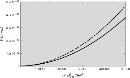
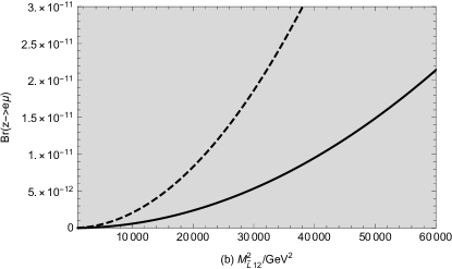
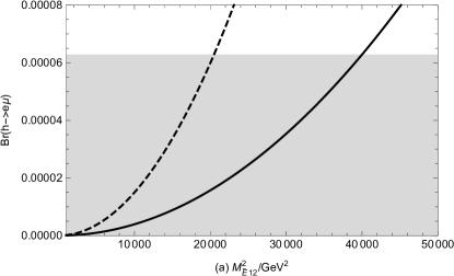
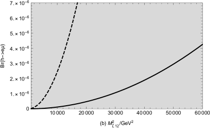
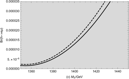
With the parameters v S = 4.3 TeV subscript 𝑣 𝑆 4.3 TeV v_{S}=4.3~{}{\rm TeV} M 1 = 1.2 TeV subscript 𝑀 1 1.2 TeV M_{1}=1.2~{}{\rm TeV} M L ~ i i 2 = 3 TeV 2 subscript superscript 𝑀 2 ~ 𝐿 𝑖 𝑖 3 superscript TeV 2 M^{2}_{\tilde{L}ii}=3~{}{\rm TeV}^{2} T e i i = 0.5 TeV subscript 𝑇 𝑒 𝑖 𝑖 0.5 TeV T_{eii}=0.5~{}{\rm TeV} T ν i i = 1 TeV subscript 𝑇 𝜈 𝑖 𝑖 1 TeV T_{{\nu}ii}=1~{}{\rm TeV} M ν ~ i i 2 = 0.3 TeV 2 subscript superscript 𝑀 2 ~ 𝜈 𝑖 𝑖 0.3 superscript TeV 2 M^{2}_{{\tilde{\nu}}ii}=0.3~{}{\rm TeV}^{2} M E ~ i i 2 = 0.8 TeV 2 subscript superscript 𝑀 2 ~ 𝐸 𝑖 𝑖 0.8 superscript TeV 2 M^{2}_{\tilde{E}ii}=0.8~{}{\rm TeV}^{2} B r ( Z → e μ ) 𝐵 𝑟 → 𝑍 𝑒 𝜇 Br(Z\rightarrow e{\mu}) 5
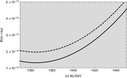
Figure 5: B r ( Z → e μ ) 𝐵 𝑟 → 𝑍 𝑒 𝜇 Br(Z\rightarrow e{\mu}) B r ( Z → e μ ) 𝐵 𝑟 → 𝑍 𝑒 𝜇 Br(Z\rightarrow e{\mu}) 5 M S = 1.5 TeV subscript 𝑀 𝑆 1.5 TeV M_{S}=1.5~{}{\rm TeV} M S = 1.2 TeV subscript 𝑀 𝑆 1.2 TeV M_{S}=1.2~{}{\rm TeV} 5 M L ~ 12 2 = 6 × 10 3 GeV 2 subscript superscript 𝑀 2 ~ 𝐿 12 6 superscript 10 3 superscript GeV 2 M^{2}_{\tilde{L}12}=6\times 10^{3}~{}{\rm GeV}^{2} M L ~ 12 2 = 5 × 10 3 GeV 2 subscript superscript 𝑀 2 ~ 𝐿 12 5 superscript 10 3 superscript GeV 2 M^{2}_{\tilde{L}12}=5\times 10^{3}~{}{\rm GeV}^{2}
In the Fig.5 B r ( Z → e μ ) 𝐵 𝑟 → 𝑍 𝑒 𝜇 Br(Z\rightarrow e{\mu}) M E ~ 12 2 subscript superscript 𝑀 2 ~ 𝐸 12 M^{2}_{\tilde{E}12} M S = 1.5 TeV subscript 𝑀 𝑆 1.5 TeV M_{S}=1.5~{}{\rm TeV} M S = 1.2 TeV subscript 𝑀 𝑆 1.2 TeV M_{S}=1.2~{}{\rm TeV} M E ~ 12 2 subscript superscript 𝑀 2 ~ 𝐸 12 M^{2}_{\tilde{E}12} 10 3 GeV 2 − 5 × 10 4 GeV 2 superscript 10 3 superscript GeV 2 5 superscript 10 4 superscript GeV 2 10^{3}~{}{\rm GeV}^{2}-5\times 10^{4}~{}{\rm GeV}^{2} 5 B r ( Z → e μ ) 𝐵 𝑟 → 𝑍 𝑒 𝜇 Br(Z\rightarrow e{\mu}) M L ~ 12 2 subscript superscript 𝑀 2 ~ 𝐿 12 M^{2}_{\tilde{L}12} M S = 1.5 TeV subscript 𝑀 𝑆 1.5 TeV M_{S}=1.5~{}{\rm TeV} M S = 1.2 TeV subscript 𝑀 𝑆 1.2 TeV M_{S}=1.2~{}{\rm TeV} M L ~ 12 2 subscript superscript 𝑀 2 ~ 𝐿 12 M^{2}_{\tilde{L}12} 10 3 GeV 2 − 6 × 10 4 GeV 2 superscript 10 3 superscript GeV 2 6 superscript 10 4 superscript GeV 2 10^{3}~{}{\rm GeV}^{2}-6\times 10^{4}~{}{\rm GeV}^{2} 5 B r ( Z → e μ ) 𝐵 𝑟 → 𝑍 𝑒 𝜇 Br(Z\rightarrow e{\mu}) M S subscript 𝑀 𝑆 M_{S} M L ~ 12 2 = 6 × 10 3 GeV 2 subscript superscript 𝑀 2 ~ 𝐿 12 6 superscript 10 3 superscript GeV 2 M^{2}_{\tilde{L}12}=6\times 10^{3}~{}{\rm GeV}^{2} M L ~ 12 2 = 5 × 10 3 GeV 2 subscript superscript 𝑀 2 ~ 𝐿 12 5 superscript 10 3 superscript GeV 2 M^{2}_{\tilde{L}12}=5\times 10^{3}~{}{\rm GeV}^{2} M S subscript 𝑀 𝑆 M_{S} 1350 GeV − 1450 GeV 1350 GeV 1450 GeV 1350~{}{\rm GeV}-1450~{}{\rm GeV} l j → l i γ → subscript 𝑙 𝑗 subscript 𝑙 𝑖 𝛾 l_{j}\rightarrow{l_{i}\gamma} T1 ; T10 U ( 1 ) X S S M 𝑈 subscript 1 𝑋 𝑆 𝑆 𝑀 U(1)_{X}SSM μ → e γ → 𝜇 𝑒 𝛾 \mu\rightarrow e\gamma
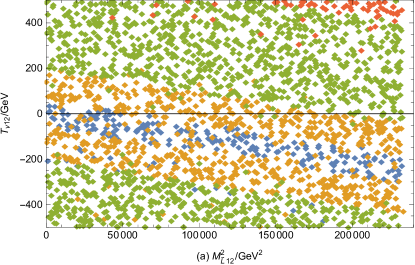
Figure 6: Under the premise of current limit on lepton flavor violating decay Z → e μ → 𝑍 𝑒 𝜇 Z\rightarrow e{\mu} < B r ( Z → e μ ) < 5 × 10 − 14 absent 𝐵 𝑟 → 𝑍 𝑒 𝜇 5 superscript 10 14 <Br(Z\rightarrow e{\mu})<5\times 10^{-14} 5 × 10 − 14 ≤ B r ( Z → e μ ) < 5 × 10 − 13 5 superscript 10 14 𝐵 𝑟 → 𝑍 𝑒 𝜇 5 superscript 10 13 5\times 10^{-14}\leq Br(Z\rightarrow e{\mu})<5\times 10^{-13} 5 × 10 − 13 5 superscript 10 13 5\times 10^{-13} ≤ B r ( Z → e μ ) < 5 × 10 − 12 absent 𝐵 𝑟 → 𝑍 𝑒 𝜇 5 superscript 10 12 \leq Br(Z\rightarrow e{\mu})<5\times 10^{-12} 5 × 10 − 12 5 superscript 10 12 5\times 10^{-12} ≤ B r ( Z → e μ ) < 7.5 × 10 − 7 absent 𝐵 𝑟 → 𝑍 𝑒 𝜇 7.5 superscript 10 7 \leq Br(Z\rightarrow e{\mu})<7.5\times 10^{-7}
In summary, M E ~ 12 2 subscript superscript 𝑀 2 ~ 𝐸 12 M^{2}_{\tilde{E}12} M L ~ 12 2 subscript superscript 𝑀 2 ~ 𝐿 12 M^{2}_{\tilde{L}12} S 𝑆 S M S subscript 𝑀 𝑆 M_{S} M E ~ 12 2 subscript superscript 𝑀 2 ~ 𝐸 12 M^{2}_{\tilde{E}12} M L ~ 12 2 subscript superscript 𝑀 2 ~ 𝐿 12 M^{2}_{\tilde{L}12} M S subscript 𝑀 𝑆 M_{S} B r ( Z → e μ ) 𝐵 𝑟 → 𝑍 𝑒 𝜇 Br(Z\rightarrow e{\mu}) M E ~ 12 2 subscript superscript 𝑀 2 ~ 𝐸 12 M^{2}_{\tilde{E}12} M L ~ 12 2 subscript superscript 𝑀 2 ~ 𝐿 12 M^{2}_{\tilde{L}12} M S subscript 𝑀 𝑆 M_{S} 5 10 − 13 − 10 − 11 superscript 10 13 superscript 10 11 10^{-13}-10^{-11} M E ~ 12 2 subscript superscript 𝑀 2 ~ 𝐸 12 M^{2}_{\tilde{E}12} M L ~ 12 2 subscript superscript 𝑀 2 ~ 𝐿 12 M^{2}_{\tilde{L}12} M S subscript 𝑀 𝑆 M_{S} B r ( Z → e μ ) 𝐵 𝑟 → 𝑍 𝑒 𝜇 Br(Z\rightarrow e{\mu})
Table 5: Scanning parameters for Fig.6 11
Next, supposing the parameters with M S = 1.2 TeV subscript 𝑀 𝑆 1.2 TeV M_{S}=1.2~{}{\rm TeV} 6 5 < B r ( Z → e μ ) < 5 × 10 − 14 absent 𝐵 𝑟 → 𝑍 𝑒 𝜇 5 superscript 10 14 <Br(Z\rightarrow e{\mu})<5\times 10^{-14} 5 × 10 − 14 ≤ B r ( Z → e μ ) < 5 × 10 − 13 5 superscript 10 14 𝐵 𝑟 → 𝑍 𝑒 𝜇 5 superscript 10 13 5\times 10^{-14}\leq Br(Z\rightarrow e{\mu})<5\times 10^{-13} 5 × 10 − 13 5 superscript 10 13 5\times 10^{-13} ≤ B r ( Z → e μ ) < 5 × 10 − 12 absent 𝐵 𝑟 → 𝑍 𝑒 𝜇 5 superscript 10 12 \leq Br(Z\rightarrow e{\mu})<5\times 10^{-12} 5 × 10 − 12 5 superscript 10 12 5\times 10^{-12} ≤ B r ( Z → e μ ) < 7.5 × 10 − 7 absent 𝐵 𝑟 → 𝑍 𝑒 𝜇 7.5 superscript 10 7 \leq Br(Z\rightarrow e{\mu})<7.5\times 10^{-7} Z → e μ → 𝑍 𝑒 𝜇 Z\rightarrow e{\mu}
The relationship between M L ~ 12 2 subscript superscript 𝑀 2 ~ 𝐿 12 M^{2}_{\tilde{L}12} T ν 12 subscript 𝑇 𝜈 12 T_{{\nu}12} 6 6 < T ν 12 < 500 absent subscript 𝑇 𝜈 12 500 <T_{{\nu}12}<500 < T ν 12 < 50 absent subscript 𝑇 𝜈 12 50 <T_{{\nu}12}<50 < T ν 12 < 200 absent subscript 𝑇 𝜈 12 200 <T_{{\nu}12}<200 < T ν 12 < − 200 absent subscript 𝑇 𝜈 12 200 <T_{{\nu}12}<-200 < T ν < 500 absent subscript 𝑇 𝜈 500 <T_{\nu}<500 < T ν 12 < 500 absent subscript 𝑇 𝜈 12 500 <T_{{\nu}12}<500
The relationship between M E ~ 12 2 subscript superscript 𝑀 2 ~ 𝐸 12 M^{2}_{\tilde{E}12} T ν 12 subscript 𝑇 𝜈 12 T_{{\nu}12} 6 M ν ~ 12 2 subscript superscript 𝑀 2 ~ 𝜈 12 M^{2}_{\tilde{\nu}12} T ν 12 subscript 𝑇 𝜈 12 T_{{\nu}12} 6 6 6 < T ν 12 < 0 absent subscript 𝑇 𝜈 12 0 <T_{{\nu}12}<0 < T ν 12 < 100 absent subscript 𝑇 𝜈 12 100 <T_{{\nu}12}<100 < T ν 12 < − 300 absent subscript 𝑇 𝜈 12 300 <T_{{\nu}12}<-300 < T ν 12 < 500 absent subscript 𝑇 𝜈 12 500 <T_{{\nu}12}<500 < T ν 12 < 500 absent subscript 𝑇 𝜈 12 500 <T_{{\nu}12}<500
V.2 Z → e τ → 𝑍 𝑒 𝜏 Z\rightarrow e{\tau}
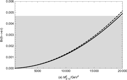
With the parameters v S = 4.3 TeV subscript 𝑣 𝑆 4.3 TeV v_{S}=4.3~{}{\rm TeV} M S = 1.2 TeV subscript 𝑀 𝑆 1.2 TeV M_{S}=1.2~{}{\rm TeV} tan β = 20 𝛽 20 \tan{\beta}=20 T e i i = 2 TeV subscript 𝑇 𝑒 𝑖 𝑖 2 TeV T_{eii}=2~{}{\rm TeV} T ν i i = 3 TeV subscript 𝑇 𝜈 𝑖 𝑖 3 TeV T_{{\nu}ii}=3~{}{\rm TeV} B r ( Z → e τ ) 𝐵 𝑟 → 𝑍 𝑒 𝜏 Br(Z\rightarrow e{\tau}) 7
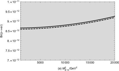
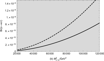
Figure 7: B r ( Z → e τ ) 𝐵 𝑟 → 𝑍 𝑒 𝜏 Br(Z\rightarrow e{\tau}) B r ( Z → e τ ) 𝐵 𝑟 → 𝑍 𝑒 𝜏 Br(Z\rightarrow e{\tau}) 7 M L ~ i i 2 = 2.5 × 10 6 GeV 2 subscript superscript 𝑀 2 ~ 𝐿 𝑖 𝑖 2.5 superscript 10 6 superscript GeV 2 M^{2}_{\tilde{L}ii}=2.5\times 10^{6}~{}{\rm GeV^{2}} M L ~ i i 2 = 3 × 10 6 GeV 2 subscript superscript 𝑀 2 ~ 𝐿 𝑖 𝑖 3 superscript 10 6 superscript GeV 2 M^{2}_{\tilde{L}ii}=3\times 10^{6}~{}{\rm GeV^{2}}
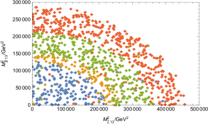
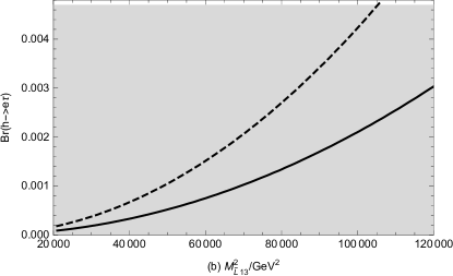
We study the branching ratio of Z → e τ → 𝑍 𝑒 𝜏 Z\rightarrow e{\tau} M E ~ 13 2 subscript superscript 𝑀 2 ~ 𝐸 13 M^{2}_{\tilde{E}13} M L ~ i i 2 = 2.5 × 10 6 GeV 2 ( 3 × 10 6 GeV 2 ) subscript superscript 𝑀 2 ~ 𝐿 𝑖 𝑖 2.5 superscript 10 6 superscript GeV 2 3 superscript 10 6 superscript GeV 2 M^{2}_{\tilde{L}ii}=2.5\times 10^{6}~{}{\rm GeV^{2}}(3\times 10^{6}~{}{\rm GeV^{2}}) 7 M E ~ 13 2 subscript superscript 𝑀 2 ~ 𝐸 13 M^{2}_{\tilde{E}13} 10 3 superscript 10 3 10^{3} GeV 2 superscript GeV 2 \rm GeV^{2} 2 × 10 4 2 superscript 10 4 2\times 10^{4} GeV 2 superscript GeV 2 \rm GeV^{2} M E ~ 13 2 subscript superscript 𝑀 2 ~ 𝐸 13 M^{2}_{\tilde{E}13} 7 Z → e τ → 𝑍 𝑒 𝜏 Z\rightarrow e{\tau} M L ~ 13 2 subscript superscript 𝑀 2 ~ 𝐿 13 M^{2}_{\tilde{L}13} M L ~ i i 2 = 2.5 × 10 6 GeV 2 subscript superscript 𝑀 2 ~ 𝐿 𝑖 𝑖 2.5 superscript 10 6 superscript GeV 2 M^{2}_{\tilde{L}ii}=2.5\times 10^{6}~{}{\rm GeV^{2}} M L ~ i i 2 = 3 × 10 6 GeV 2 subscript superscript 𝑀 2 ~ 𝐿 𝑖 𝑖 3 superscript 10 6 superscript GeV 2 M^{2}_{\tilde{L}ii}=3\times 10^{6}~{}{\rm GeV^{2}} M L ~ 13 2 subscript superscript 𝑀 2 ~ 𝐿 13 M^{2}_{\tilde{L}13} 2 × 10 3 2 superscript 10 3 2\times 10^{3} GeV 2 superscript GeV 2 \rm GeV^{2} 1.2 × 10 4 1.2 superscript 10 4 1.2\times 10^{4} GeV 2 superscript GeV 2 \rm GeV^{2} M E ~ 13 2 subscript superscript 𝑀 2 ~ 𝐸 13 M^{2}_{\tilde{E}13} M L ~ 13 2 subscript superscript 𝑀 2 ~ 𝐿 13 M^{2}_{\tilde{L}13}
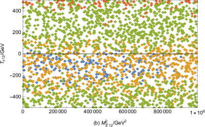
Next, supposing M S = 1.2 TeV subscript 𝑀 𝑆 1.2 TeV M_{S}=1.2~{}{\rm TeV} Z → e τ → 𝑍 𝑒 𝜏 Z\rightarrow e{\tau} 8 tan β 𝛽 \tan\beta M 1 subscript 𝑀 1 M_{1} M 2 subscript 𝑀 2 M_{2} M L ~ i i 2 subscript superscript 𝑀 2 ~ 𝐿 𝑖 𝑖 M^{2}_{\tilde{L}ii} M E ~ i i 2 subscript superscript 𝑀 2 ~ 𝐸 𝑖 𝑖 M^{2}_{\tilde{E}ii} M ν ~ i i 2 subscript superscript 𝑀 2 ~ 𝜈 𝑖 𝑖 M^{2}_{{\tilde{\nu}}ii} T e i i subscript 𝑇 𝑒 𝑖 𝑖 T_{eii} T ν i i subscript 𝑇 𝜈 𝑖 𝑖 T_{{\nu}ii} 5 6 < B r ( Z → e τ ) < 7 × 10 − 15 absent 𝐵 𝑟 → 𝑍 𝑒 𝜏 7 superscript 10 15 <Br(Z\rightarrow e{\tau})<7\times 10^{-15} 7 × 10 − 15 ≤ B r ( Z → e τ ) < 1 × 10 − 14 7 superscript 10 15 𝐵 𝑟 → 𝑍 𝑒 𝜏 1 superscript 10 14 7\times 10^{-15}\leq Br(Z\rightarrow e{\tau})<1\times 10^{-14} 1 × 10 − 14 1 superscript 10 14 1\times 10^{-14} ≤ B r ( Z → e τ ) < 2 × 10 − 14 absent 𝐵 𝑟 → 𝑍 𝑒 𝜏 2 superscript 10 14 \leq Br(Z\rightarrow e{\tau})<2\times 10^{-14} 2 × 10 − 14 2 superscript 10 14 2\times 10^{-14} ≤ B r ( Z → e τ ) < 9.8 × 10 − 6 absent 𝐵 𝑟 → 𝑍 𝑒 𝜏 9.8 superscript 10 6 \leq Br(Z\rightarrow e{\tau})<9.8\times 10^{-6} Z → e τ → 𝑍 𝑒 𝜏 Z\rightarrow e{\tau}
Table 6: Scanning parameters for Fig.8 13
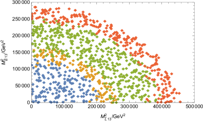
Figure 8: Under the premise of current limit on lepton flavor violating decay Z → e τ → 𝑍 𝑒 𝜏 Z\rightarrow e{\tau} < B r ( Z → e τ ) < 7 × 10 − 15 absent 𝐵 𝑟 → 𝑍 𝑒 𝜏 7 superscript 10 15 <Br(Z\rightarrow e{\tau})<7\times 10^{-15} 7 × 10 − 15 ≤ B r ( Z → e τ ) < 1 × 10 − 14 7 superscript 10 15 𝐵 𝑟 → 𝑍 𝑒 𝜏 1 superscript 10 14 7\times 10^{-15}\leq Br(Z\rightarrow e{\tau})<1\times 10^{-14} 1 × 10 − 14 1 superscript 10 14 1\times 10^{-14} ≤ B r ( Z → e τ ) < 2 × 10 − 14 absent 𝐵 𝑟 → 𝑍 𝑒 𝜏 2 superscript 10 14 \leq Br(Z\rightarrow e{\tau})<2\times 10^{-14} 2 × 10 − 14 2 superscript 10 14 2\times 10^{-14} ≤ B r ( Z → e τ ) < 9.8 × 10 − 6 absent 𝐵 𝑟 → 𝑍 𝑒 𝜏 9.8 superscript 10 6 \leq Br(Z\rightarrow e{\tau})<9.8\times 10^{-6}
The analysis of the relationship between M L ~ 13 2 subscript superscript 𝑀 2 ~ 𝐿 13 M^{2}_{\tilde{L}13} M E ~ 13 2 subscript superscript 𝑀 2 ~ 𝐸 13 M^{2}_{\tilde{E}13} 8 8 0 GeV 2 < M E ~ 13 2 < 3 × 10 5 GeV 2 0 superscript GeV 2 subscript superscript 𝑀 2 ~ 𝐸 13 3 superscript 10 5 superscript GeV 2 0~{}{\rm GeV}^{2}<M^{2}_{\tilde{E}13}<3\times 10^{5}~{}{\rm GeV}^{2} 0 GeV 2 < M L ~ 13 2 < 2.2 × 10 5 GeV 2 0 superscript GeV 2 subscript superscript 𝑀 2 ~ 𝐿 13 2.2 superscript 10 5 superscript GeV 2 0~{}{\rm GeV}^{2}<M^{2}_{\tilde{L}13}<2.2\times 10^{5}~{}{\rm GeV}^{2} 0 GeV 2 < M E ~ 13 2 < 1.25 × 10 5 GeV 2 0 superscript GeV 2 subscript superscript 𝑀 2 ~ 𝐸 13 1.25 superscript 10 5 superscript GeV 2 0~{}{\rm GeV}^{2}<M^{2}_{\tilde{E}13}<1.25\times 10^{5}~{}{\rm GeV}^{2} 2.2 × 10 5 GeV 2 < M L ~ 13 2 < 2.6 × 10 5 GeV 2 2.2 superscript 10 5 superscript GeV 2 subscript superscript 𝑀 2 ~ 𝐿 13 2.6 superscript 10 5 superscript GeV 2 2.2\times 10^{5}~{}{\rm GeV}^{2}<M^{2}_{\tilde{L}13}<2.6\times 10^{5}~{}{\rm GeV}^{2} 1.25 × 10 5 GeV 2 < M E ~ 13 2 < 1.5 × 10 5 GeV 2 1.25 superscript 10 5 superscript GeV 2 subscript superscript 𝑀 2 ~ 𝐸 13 1.5 superscript 10 5 superscript GeV 2 1.25\times 10^{5}~{}{\rm GeV}^{2}<M^{2}_{\tilde{E}13}<1.5\times 10^{5}~{}{\rm GeV}^{2} 2.6 × 10 5 GeV 2 < M L ~ 13 2 < 3.6 × 10 5 GeV 2 2.6 superscript 10 5 superscript GeV 2 subscript superscript 𝑀 2 ~ 𝐿 13 3.6 superscript 10 5 superscript GeV 2 2.6\times 10^{5}~{}{\rm GeV}^{2}<M^{2}_{\tilde{L}13}<3.6\times 10^{5}~{}{\rm GeV}^{2} 1.5 × 10 5 GeV 2 < M E ~ 13 2 < 2.1 × 10 5 GeV 2 1.5 superscript 10 5 superscript GeV 2 subscript superscript 𝑀 2 ~ 𝐸 13 2.1 superscript 10 5 superscript GeV 2 1.5\times 10^{5}~{}{\rm GeV}^{2}<M^{2}_{\tilde{E}13}<2.1\times 10^{5}~{}{\rm GeV}^{2} 3.6 × 10 5 GeV 2 < M L ~ 13 2 < 4.6 × 10 5 GeV 2 3.6 superscript 10 5 superscript GeV 2 subscript superscript 𝑀 2 ~ 𝐿 13 4.6 superscript 10 5 superscript GeV 2 3.6\times 10^{5}~{}{\rm GeV}^{2}<M^{2}_{\tilde{L}13}<4.6\times 10^{5}~{}{\rm GeV}^{2} 2.1 × 10 5 GeV 2 < M E ~ 13 2 < 3 × 10 5 GeV 2 2.1 superscript 10 5 superscript GeV 2 subscript superscript 𝑀 2 ~ 𝐸 13 3 superscript 10 5 superscript GeV 2 2.1\times 10^{5}~{}{\rm GeV}^{2}<M^{2}_{\tilde{E}13}<3\times 10^{5}~{}{\rm GeV}^{2}
V.3 Z → μ τ → 𝑍 𝜇 𝜏 Z\rightarrow{\mu}{\tau}
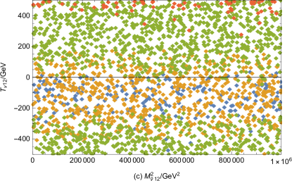
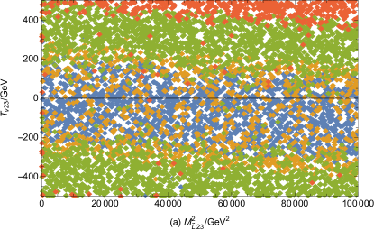
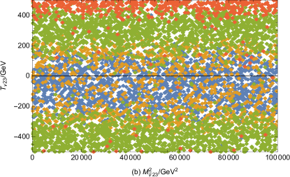
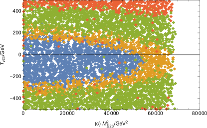
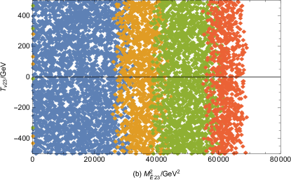
The experimental upper bound for the LFV process Z → μ τ → 𝑍 𝜇 𝜏 Z\rightarrow{\mu}{\tau} 1.2 × 10 − 5 1.2 superscript 10 5 1.2\times 10^{-5} Z → e μ → 𝑍 𝑒 𝜇 Z\rightarrow e{\mu} M E ~ 23 2 subscript superscript 𝑀 2 ~ 𝐸 23 M^{2}_{\tilde{E}23} M L ~ 23 2 subscript superscript 𝑀 2 ~ 𝐿 23 M^{2}_{\tilde{L}23} T ν 23 subscript 𝑇 𝜈 23 T_{{\nu}23} Z → μ τ → 𝑍 𝜇 𝜏 Z\rightarrow{\mu}{\tau} Z → e μ → 𝑍 𝑒 𝜇 Z\rightarrow e{\mu} Z → e τ → 𝑍 𝑒 𝜏 Z\rightarrow e{\tau} M E ~ 23 2 subscript superscript 𝑀 2 ~ 𝐸 23 M^{2}_{\tilde{E}23} M L ~ 23 2 subscript superscript 𝑀 2 ~ 𝐿 23 M^{2}_{\tilde{L}23} T ν 23 subscript 𝑇 𝜈 23 T_{{\nu}23} M E ~ 23 2 subscript superscript 𝑀 2 ~ 𝐸 23 M^{2}_{\tilde{E}23} Z → μ τ → 𝑍 𝜇 𝜏 Z\rightarrow{\mu}{\tau} 10 − 13 superscript 10 13 10^{-13} M L ~ 23 2 subscript superscript 𝑀 2 ~ 𝐿 23 M^{2}_{\tilde{L}23} Z → μ τ → 𝑍 𝜇 𝜏 Z\rightarrow{\mu}{\tau} 10 − 11 superscript 10 11 10^{-11} T ν 23 subscript 𝑇 𝜈 23 T_{{\nu}23} Z → μ τ → 𝑍 𝜇 𝜏 Z\rightarrow{\mu}{\tau} 10 − 9 superscript 10 9 10^{-9} T ν 23 subscript 𝑇 𝜈 23 T_{{\nu}23} M E ~ 23 2 subscript superscript 𝑀 2 ~ 𝐸 23 M^{2}_{\tilde{E}23} M L ~ 23 2 subscript superscript 𝑀 2 ~ 𝐿 23 M^{2}_{\tilde{L}23}
Figure 9: Under the premise of current limit on lepton flavor violating decay Z → μ τ → 𝑍 𝜇 𝜏 Z\rightarrow{\mu}{\tau} < B r ( Z → μ τ ) < 6 × 10 − 13 absent 𝐵 𝑟 → 𝑍 𝜇 𝜏 6 superscript 10 13 <Br(Z\rightarrow{\mu}{\tau})<6\times 10^{-13} 6 × 10 − 13 ≤ B r ( Z → μ τ ) < 10 − 12 6 superscript 10 13 𝐵 𝑟 → 𝑍 𝜇 𝜏 superscript 10 12 6\times 10^{-13}\leq Br(Z\rightarrow{\mu}{\tau})<10^{-12} 10 − 12 superscript 10 12 10^{-12} ≤ B r ( Z → μ τ ) < 3 × 10 − 12 absent 𝐵 𝑟 → 𝑍 𝜇 𝜏 3 superscript 10 12 \leq Br(Z\rightarrow{\mu}{\tau})<3\times 10^{-12} 3 × 10 − 12 3 superscript 10 12 3\times 10^{-12} ≤ B r ( Z → μ τ ) < 1.2 × 10 − 5 absent 𝐵 𝑟 → 𝑍 𝜇 𝜏 1.2 superscript 10 5 \leq Br(Z\rightarrow{\mu}{\tau})<1.2\times 10^{-5}
Next, we scatter points on Z → μ τ → 𝑍 𝜇 𝜏 Z\rightarrow{\mu}{\tau} 9 7 < B r ( Z → μ τ ) < 6 × 10 − 13 absent 𝐵 𝑟 → 𝑍 𝜇 𝜏 6 superscript 10 13 <Br(Z\rightarrow{\mu}{\tau})<6\times 10^{-13} 6 × 10 − 13 ≤ B r ( Z → μ τ ) < 10 − 12 6 superscript 10 13 𝐵 𝑟 → 𝑍 𝜇 𝜏 superscript 10 12 6\times 10^{-13}\leq Br(Z\rightarrow{\mu}{\tau})<10^{-12} 10 − 12 superscript 10 12 10^{-12} ≤ B r ( Z → μ τ ) < 3 × 10 − 12 absent 𝐵 𝑟 → 𝑍 𝜇 𝜏 3 superscript 10 12 \leq Br(Z\rightarrow{\mu}{\tau})<3\times 10^{-12} 3 × 10 − 12 3 superscript 10 12 3\times 10^{-12} ≤ B r ( Z → μ τ ) < 1.2 × 10 − 5 absent 𝐵 𝑟 → 𝑍 𝜇 𝜏 1.2 superscript 10 5 \leq Br(Z\rightarrow{\mu}{\tau})<1.2\times 10^{-5} Z → μ τ → 𝑍 𝜇 𝜏 Z\rightarrow{\mu}{\tau}
Table 7: Scanning parameters for Fig.9
The analysis of the relationship between M L ~ 23 2 subscript superscript 𝑀 2 ~ 𝐿 23 M^{2}_{\tilde{L}23} T ν 23 subscript 𝑇 𝜈 23 T_{{\nu}23} M ν ~ 23 2 subscript superscript 𝑀 2 ~ 𝜈 23 M^{2}_{\tilde{\nu}23} T ν 23 subscript 𝑇 𝜈 23 T_{{\nu}23} M E ~ 23 2 subscript superscript 𝑀 2 ~ 𝐸 23 M^{2}_{\tilde{E}23} T ν 23 subscript 𝑇 𝜈 23 T_{{\nu}23} 9 9 < T ν 23 < 500 absent subscript 𝑇 𝜈 23 500 <T_{{\nu}23}<500 9 < T ν 23 < 180 absent subscript 𝑇 𝜈 23 180 <T_{{\nu}23}<180 < T ν 23 < 200 absent subscript 𝑇 𝜈 23 200 <T_{{\nu}23}<200 < T ν 23 < − 200 absent subscript 𝑇 𝜈 23 200 <T_{{\nu}23}<-200 < T ν 23 < 400 absent subscript 𝑇 𝜈 23 400 <T_{{\nu}23}<400 < T ν 23 < 500 absent subscript 𝑇 𝜈 23 500 <T_{{\nu}23}<500 9 < T ν 23 < 180 absent subscript 𝑇 𝜈 23 180 <T_{{\nu}23}<180 < T ν 23 < 200 absent subscript 𝑇 𝜈 23 200 <T_{{\nu}23}<200 < T ν 23 < − 200 absent subscript 𝑇 𝜈 23 200 <T_{{\nu}23}<-200 < T ν 23 < 400 absent subscript 𝑇 𝜈 23 400 <T_{{\nu}23}<400 < T ν 23 < 500 absent subscript 𝑇 𝜈 23 500 <T_{{\nu}23}<500 9 9 9 9
Finally, we analyze the effect from parameters M E ~ 23 2 subscript superscript 𝑀 2 ~ 𝐸 23 M^{2}_{\tilde{E}23} T ν 23 subscript 𝑇 𝜈 23 T_{{\nu}23} 9 T ν 23 = 0 subscript 𝑇 𝜈 23 0 T_{{\nu}23}=0 < T ν 23 < 200 absent subscript 𝑇 𝜈 23 200 <T_{{\nu}23}<200 0 GeV 2 < M E ~ 23 2 < 5.5 × 10 4 GeV 2 0 superscript GeV 2 subscript superscript 𝑀 2 ~ 𝐸 23 5.5 superscript 10 4 superscript GeV 2 0~{}{\rm GeV}^{2}<M^{2}_{\tilde{E}23}<5.5\times 10^{4}~{}{\rm GeV}^{2} < T ν 23 < − 300 absent subscript 𝑇 𝜈 23 300 <T_{{\nu}23}<-300 < T ν 23 < 400 absent subscript 𝑇 𝜈 23 400 <T_{{\nu}23}<400 < T ν 23 < 500 absent subscript 𝑇 𝜈 23 500 <T_{{\nu}23}<500
V.4 h → e μ → ℎ 𝑒 𝜇 h\rightarrow e{\mu}
In this subsection, we mainly analyze 125 GeV Higgs boson decays with LFV h → e μ → ℎ 𝑒 𝜇 h\rightarrow e{\mu} U ( 1 ) X 𝑈 subscript 1 𝑋 U(1)_{X} Z → e μ → 𝑍 𝑒 𝜇 Z\rightarrow e{\mu} B r ( h → e μ ) 𝐵 𝑟 → ℎ 𝑒 𝜇 Br(h\rightarrow e{\mu}) 10
Figure 10: B r ( h → e μ ) 𝐵 𝑟 → ℎ 𝑒 𝜇 Br(h\rightarrow e{\mu}) B r ( h → e μ ) 𝐵 𝑟 → ℎ 𝑒 𝜇 Br(h\rightarrow e{\mu}) 10 M S = 1.5 TeV subscript 𝑀 𝑆 1.5 TeV M_{S}=1.5~{}{\rm TeV} M S = 1.2 TeV subscript 𝑀 𝑆 1.2 TeV M_{S}=1.2~{}{\rm TeV} 10 M L ~ 12 2 = 6 × 10 3 GeV 2 subscript superscript 𝑀 2 ~ 𝐿 12 6 superscript 10 3 superscript GeV 2 M^{2}_{\tilde{L}12}=6\times 10^{3}~{}{\rm GeV}^{2} M L ~ 12 2 = 5 × 10 3 GeV 2 subscript superscript 𝑀 2 ~ 𝐿 12 5 superscript 10 3 superscript GeV 2 M^{2}_{\tilde{L}12}=5\times 10^{3}~{}{\rm GeV}^{2}
In the Fig.10 B r ( h → e μ ) 𝐵 𝑟 → ℎ 𝑒 𝜇 Br(h\rightarrow e{\mu}) M E ~ 12 2 subscript superscript 𝑀 2 ~ 𝐸 12 M^{2}_{\tilde{E}12} M S = 1.5 TeV subscript 𝑀 𝑆 1.5 TeV M_{S}=1.5~{}{\rm TeV} M S = 1.2 TeV subscript 𝑀 𝑆 1.2 TeV M_{S}=1.2~{}{\rm TeV} B r ( h → e μ ) 𝐵 𝑟 → ℎ 𝑒 𝜇 Br(h\rightarrow e{\mu}) M E ~ 12 2 subscript superscript 𝑀 2 ~ 𝐸 12 M^{2}_{\tilde{E}12} 0 GeV 2 0 superscript GeV 2 0~{}{\rm GeV}^{2} 5 × 10 4 GeV 2 5 superscript 10 4 superscript GeV 2 5\times 10^{4}~{}{\rm GeV}^{2} 0 GeV 2 0 superscript GeV 2 0~{}{\rm GeV}^{2} 2 × 10 4 GeV 2 2 superscript 10 4 superscript GeV 2 2\times 10^{4}~{}{\rm GeV}^{2} 0 GeV 2 0 superscript GeV 2 0~{}{\rm GeV}^{2} 4 × 10 4 GeV 2 4 superscript 10 4 superscript GeV 2 4\times 10^{4}~{}{\rm GeV}^{2}
In the Fig.10 B r ( h → e μ ) 𝐵 𝑟 → ℎ 𝑒 𝜇 Br(h\rightarrow e{\mu}) M L ~ 12 2 subscript superscript 𝑀 2 ~ 𝐿 12 M^{2}_{\tilde{L}12} M S = 1.5 TeV subscript 𝑀 𝑆 1.5 TeV M_{S}=1.5~{}{\rm TeV} M S = 1.2 TeV subscript 𝑀 𝑆 1.2 TeV M_{S}=1.2~{}{\rm TeV} M L ~ 12 2 subscript superscript 𝑀 2 ~ 𝐿 12 M^{2}_{\tilde{L}12} 0 GeV 2 0 superscript GeV 2 0~{}{\rm GeV}^{2} 2 × 10 4 GeV 2 2 superscript 10 4 superscript GeV 2 2\times 10^{4}~{}{\rm GeV}^{2} M L ~ 12 2 subscript superscript 𝑀 2 ~ 𝐿 12 M^{2}_{\tilde{L}12} 0 GeV 2 0 superscript GeV 2 0~{}{\rm GeV}^{2} 5 × 10 4 GeV 2 5 superscript 10 4 superscript GeV 2 5\times 10^{4}~{}{\rm GeV}^{2} M E ~ 12 2 subscript superscript 𝑀 2 ~ 𝐸 12 M^{2}_{\tilde{E}12} M L ~ 12 2 subscript superscript 𝑀 2 ~ 𝐿 12 M^{2}_{\tilde{L}12}
B r ( h → e μ ) 𝐵 𝑟 → ℎ 𝑒 𝜇 Br(h\rightarrow e{\mu}) M S subscript 𝑀 𝑆 M_{S} 10 M L ~ 12 2 = 6 × 10 3 GeV 2 subscript superscript 𝑀 2 ~ 𝐿 12 6 superscript 10 3 superscript GeV 2 M^{2}_{\tilde{L}12}=6\times 10^{3}~{}{\rm GeV}^{2} M L ~ 12 2 = 5 × 10 3 GeV 2 subscript superscript 𝑀 2 ~ 𝐿 12 5 superscript 10 3 superscript GeV 2 M^{2}_{\tilde{L}12}=5\times 10^{3}~{}{\rm GeV}^{2} M S subscript 𝑀 𝑆 M_{S} 1350 GeV 1350 GeV 1350~{}{\rm GeV} 1450 GeV 1450 GeV 1450~{}{\rm GeV} 3.0 × 10 − 5 3.0 superscript 10 5 3.0\times 10^{-5} M E ~ 12 2 subscript superscript 𝑀 2 ~ 𝐸 12 M^{2}_{\tilde{E}12} M L ~ 12 2 subscript superscript 𝑀 2 ~ 𝐿 12 M^{2}_{\tilde{L}12} B r ( h → e μ ) 𝐵 𝑟 → ℎ 𝑒 𝜇 Br(h\rightarrow e{\mu}) M S subscript 𝑀 𝑆 M_{S}
Figure 11: Under the premise of current limit on lepton flavor violating decay h → e μ → ℎ 𝑒 𝜇 h\rightarrow e{\mu} < B r ( h → e μ ) < 2 × 10 − 5 absent 𝐵 𝑟 → ℎ 𝑒 𝜇 2 superscript 10 5 <Br(h\rightarrow e{\mu})<2\times 10^{-5} 2 × 10 − 5 ≤ B r ( h → e μ ) < 3 × 10 − 5 2 superscript 10 5 𝐵 𝑟 → ℎ 𝑒 𝜇 3 superscript 10 5 2\times 10^{-5}\leq Br(h\rightarrow e{\mu})<3\times 10^{-5} 3 × 10 − 5 3 superscript 10 5 3\times 10^{-5} ≤ B r ( h → e μ ) < 5 × 10 − 5 absent 𝐵 𝑟 → ℎ 𝑒 𝜇 5 superscript 10 5 \leq Br(h\rightarrow e{\mu})<5\times 10^{-5} 5 × 10 − 5 5 superscript 10 5 5\times 10^{-5} ≤ B r ( h → e μ ) < 6.28 × 10 − 5 absent 𝐵 𝑟 → ℎ 𝑒 𝜇 6.28 superscript 10 5 \leq Br(h\rightarrow e{\mu})<6.28\times 10^{-5}
Supposing M S = 1.2 TeV subscript 𝑀 𝑆 1.2 TeV M_{S}=1.2~{}{\rm TeV} M 1 = 1.2 TeV subscript 𝑀 1 1.2 TeV M_{1}=1.2~{}{\rm TeV} 5 11 < B r ( h → e μ ) < 2 × 10 − 5 absent 𝐵 𝑟 → ℎ 𝑒 𝜇 2 superscript 10 5 <Br(h\rightarrow e{\mu})<2\times 10^{-5} 2 × 10 − 5 ≤ B r ( h → e μ ) < 3 × 10 − 5 2 superscript 10 5 𝐵 𝑟 → ℎ 𝑒 𝜇 3 superscript 10 5 2\times 10^{-5}\leq Br(h\rightarrow e{\mu})<3\times 10^{-5} 3 × 10 − 5 3 superscript 10 5 3\times 10^{-5} ≤ B r ( h → e μ ) < 5 × 10 − 5 absent 𝐵 𝑟 → ℎ 𝑒 𝜇 5 superscript 10 5 \leq Br(h\rightarrow e{\mu})<5\times 10^{-5} 5 × 10 − 5 5 superscript 10 5 5\times 10^{-5} ≤ B r ( h → e μ ) < 6.28 × 10 − 5 absent 𝐵 𝑟 → ℎ 𝑒 𝜇 6.28 superscript 10 5 \leq Br(h\rightarrow e{\mu})<6.28\times 10^{-5} Z → e μ → 𝑍 𝑒 𝜇 Z\rightarrow e{\mu}
The relationship between M L ~ 12 2 subscript superscript 𝑀 2 ~ 𝐿 12 M^{2}_{\tilde{L}12} M ν 12 2 subscript superscript 𝑀 2 𝜈 12 M^{2}_{{\nu}12} 11 M L ~ 12 2 subscript superscript 𝑀 2 ~ 𝐿 12 M^{2}_{\tilde{L}12} T ν 12 subscript 𝑇 𝜈 12 T_{{\nu}12} 11 0 GeV 2 < M L ~ 12 2 < 2.3 × 10 5 GeV 2 0 superscript GeV 2 subscript superscript 𝑀 2 ~ 𝐿 12 2.3 superscript 10 5 superscript GeV 2 0~{}{\rm GeV}^{2}<M^{2}_{\tilde{L}12}<2.3\times 10^{5}~{}{\rm GeV}^{2} 0 GeV 2 < M E ~ 12 2 < 1.3 × 10 5 GeV 2 0 superscript GeV 2 subscript superscript 𝑀 2 ~ 𝐸 12 1.3 superscript 10 5 superscript GeV 2 0~{}{\rm GeV}^{2}<M^{2}_{\tilde{E}12}<1.3\times 10^{5}~{}{\rm GeV}^{2} 1.3 × 10 5 GeV 2 < M E ~ 12 2 < 1.6 × 10 5 GeV 2 1.3 superscript 10 5 superscript GeV 2 subscript superscript 𝑀 2 ~ 𝐸 12 1.6 superscript 10 5 superscript GeV 2 1.3\times 10^{5}~{}{\rm GeV}^{2}<M^{2}_{\tilde{E}12}<1.6\times 10^{5}~{}{\rm GeV}^{2} 1.6 × 10 5 GeV 2 < M E ~ 12 2 < 2.1 × 10 5 GeV 2 1.6 superscript 10 5 superscript GeV 2 subscript superscript 𝑀 2 ~ 𝐸 12 2.1 superscript 10 5 superscript GeV 2 1.6\times 10^{5}~{}{\rm GeV}^{2}<M^{2}_{\tilde{E}12}<2.1\times 10^{5}~{}{\rm GeV}^{2} 2.1 × 10 5 GeV 2 < M E ~ 12 2 < 2.3 × 10 5 GeV 2 2.1 superscript 10 5 superscript GeV 2 subscript superscript 𝑀 2 ~ 𝐸 12 2.3 superscript 10 5 superscript GeV 2 2.1\times 10^{5}~{}{\rm GeV}^{2}<M^{2}_{\tilde{E}12}<2.3\times 10^{5}~{}{\rm GeV}^{2}
V.5 h → e τ → ℎ 𝑒 𝜏 h\rightarrow e{\tau}
In this section, we analyze the 125 GeV Higgs boson decay h → e τ → ℎ 𝑒 𝜏 h\rightarrow e{\tau} U ( 1 ) X 𝑈 subscript 1 𝑋 U(1)_{X} Z → e τ → 𝑍 𝑒 𝜏 Z\rightarrow e{\tau} B r ( h → e τ ) 𝐵 𝑟 → ℎ 𝑒 𝜏 Br(h\rightarrow e{\tau}) 12
Figure 12: B r ( h → e τ ) 𝐵 𝑟 → ℎ 𝑒 𝜏 Br(h\rightarrow e{\tau}) B r ( Z → e τ ) 𝐵 𝑟 → 𝑍 𝑒 𝜏 Br(Z\rightarrow e{\tau}) 12 M L ~ i i 2 = 2.5 × 10 6 GeV 2 subscript superscript 𝑀 2 ~ 𝐿 𝑖 𝑖 2.5 superscript 10 6 superscript GeV 2 M^{2}_{\tilde{L}ii}=2.5\times 10^{6}~{}{\rm GeV}^{2} M L ~ i i 2 = 3 × 10 6 GeV 2 subscript superscript 𝑀 2 ~ 𝐿 𝑖 𝑖 3 superscript 10 6 superscript GeV 2 M^{2}_{\tilde{L}ii}=3\times 10^{6}~{}{\rm GeV}^{2}
Setting v S = 4.3 TeV subscript 𝑣 𝑆 4.3 TeV v_{S}=4.3~{}{\rm TeV} B r ( h → e τ ) 𝐵 𝑟 → ℎ 𝑒 𝜏 Br(h\rightarrow e{\tau}) M E ~ 13 2 subscript superscript 𝑀 2 ~ 𝐸 13 M^{2}_{\tilde{E}13} 12 M L ~ i i 2 = 2.5 × 10 6 GeV 2 subscript superscript 𝑀 2 ~ 𝐿 𝑖 𝑖 2.5 superscript 10 6 superscript GeV 2 M^{2}_{\tilde{L}ii}=2.5\times 10^{6}~{}{\rm GeV}^{2} M L ~ i i 2 = 3 × 10 6 GeV 2 subscript superscript 𝑀 2 ~ 𝐿 𝑖 𝑖 3 superscript 10 6 superscript GeV 2 M^{2}_{\tilde{L}ii}=3\times 10^{6}~{}{\rm GeV}^{2} M E ~ 13 2 subscript superscript 𝑀 2 ~ 𝐸 13 M^{2}_{\tilde{E}13} 0 GeV 2 − 2 × 10 4 GeV 2 0 superscript GeV 2 2 superscript 10 4 superscript GeV 2 0~{}{\rm GeV}^{2}-2\times 10^{4}~{}{\rm GeV}^{2} 0 GeV 2 < M E ~ 13 2 < 1.96 × 10 4 GeV 2 0 superscript GeV 2 subscript superscript 𝑀 2 ~ 𝐸 13 1.96 superscript 10 4 superscript GeV 2 0~{}{\rm GeV}^{2}<M^{2}_{\tilde{E}13}<1.96\times 10^{4}~{}{\rm GeV}^{2} 0 GeV 2 < M E ~ 13 2 < 1.9 × 10 4 GeV 2 0 superscript GeV 2 subscript superscript 𝑀 2 ~ 𝐸 13 1.9 superscript 10 4 superscript GeV 2 0~{}{\rm GeV}^{2}<M^{2}_{\tilde{E}13}<1.9\times 10^{4}~{}{\rm GeV}^{2}
In the Fig.12 h → e τ → ℎ 𝑒 𝜏 h\rightarrow e{\tau} M L ~ 13 2 subscript superscript 𝑀 2 ~ 𝐿 13 M^{2}_{\tilde{L}13} M L ~ i i 2 = 2.5 × 10 6 GeV 2 subscript superscript 𝑀 2 ~ 𝐿 𝑖 𝑖 2.5 superscript 10 6 superscript GeV 2 M^{2}_{\tilde{L}ii}=2.5\times 10^{6}~{}{\rm GeV}^{2} M L ~ i i 2 = 3 × 10 6 GeV 2 subscript superscript 𝑀 2 ~ 𝐿 𝑖 𝑖 3 superscript 10 6 superscript GeV 2 M^{2}_{\tilde{L}ii}=3\times 10^{6}~{}{\rm GeV}^{2} 2 × 10 3 GeV 2 < M L ~ 13 2 < 1.2 × 10 5 GeV 2 2 superscript 10 3 superscript GeV 2 subscript superscript 𝑀 2 ~ 𝐿 13 1.2 superscript 10 5 superscript GeV 2 2\times 10^{3}~{}{\rm GeV}^{2}<M^{2}_{\tilde{L}13}<1.2\times 10^{5}~{}{\rm GeV}^{2} 2 × 10 3 GeV 2 < M L ~ 13 2 < 1.05 × 10 5 GeV 2 2 superscript 10 3 superscript GeV 2 subscript superscript 𝑀 2 ~ 𝐿 13 1.05 superscript 10 5 superscript GeV 2 2\times 10^{3}~{}{\rm GeV}^{2}<M^{2}_{\tilde{L}13}<1.05\times 10^{5}~{}{\rm GeV}^{2} M E ~ 13 2 subscript superscript 𝑀 2 ~ 𝐸 13 M^{2}_{\tilde{E}13} M L ~ 13 2 subscript superscript 𝑀 2 ~ 𝐿 13 M^{2}_{\tilde{L}13}
Next, supposing the parameters with M S = 1.2 TeV subscript 𝑀 𝑆 1.2 TeV M_{S}=1.2~{}{\rm TeV} h → e τ → ℎ 𝑒 𝜏 h\rightarrow e{\tau} 13 tan β 𝛽 \tan\beta M 1 subscript 𝑀 1 M_{1} M 2 subscript 𝑀 2 M_{2} M L ~ i i 2 subscript superscript 𝑀 2 ~ 𝐿 𝑖 𝑖 M^{2}_{\tilde{L}ii} M E ~ i i 2 subscript superscript 𝑀 2 ~ 𝐸 𝑖 𝑖 M^{2}_{\tilde{E}ii} M ν ~ i i 2 subscript superscript 𝑀 2 ~ 𝜈 𝑖 𝑖 M^{2}_{{\tilde{\nu}}ii} T e i i subscript 𝑇 𝑒 𝑖 𝑖 T_{eii} T ν i i subscript 𝑇 𝜈 𝑖 𝑖 T_{{\nu}ii} 5 6 < B r ( h → e τ ) < 10 − 3 absent 𝐵 𝑟 → ℎ 𝑒 𝜏 superscript 10 3 <Br(h\rightarrow e{\tau})<10^{-3} 10 − 3 ≤ B r ( h → e τ ) < 1.5 × 10 − 3 superscript 10 3 𝐵 𝑟 → ℎ 𝑒 𝜏 1.5 superscript 10 3 10^{-3}\leq Br(h\rightarrow e{\tau})<1.5\times 10^{-3} 1.5 × 10 − 3 1.5 superscript 10 3 1.5\times 10^{-3} ≤ B r ( h → e τ ) < 3.5 × 10 − 3 absent 𝐵 𝑟 → ℎ 𝑒 𝜏 3.5 superscript 10 3 \leq Br(h\rightarrow e{\tau})<3.5\times 10^{-3} 3.5 × 10 − 3 3.5 superscript 10 3 3.5\times 10^{-3} ≤ B r ( h → e τ ) < 4.7 × 10 − 3 absent 𝐵 𝑟 → ℎ 𝑒 𝜏 4.7 superscript 10 3 \leq Br(h\rightarrow e{\tau})<4.7\times 10^{-3} h → e τ → ℎ 𝑒 𝜏 h\rightarrow e{\tau}
Figure 13: Under the premise of current limit on lepton flavor violating decay h → e τ → ℎ 𝑒 𝜏 h\rightarrow e{\tau} < B r ( h → e τ ) < 10 − 3 absent 𝐵 𝑟 → ℎ 𝑒 𝜏 superscript 10 3 <Br(h\rightarrow e{\tau})<10^{-3} 10 − 3 ≤ B r ( h → e τ ) < 1.5 × 10 − 3 superscript 10 3 𝐵 𝑟 → ℎ 𝑒 𝜏 1.5 superscript 10 3 10^{-3}\leq Br(h\rightarrow e{\tau})<1.5\times 10^{-3} 1.5 × 10 − 3 1.5 superscript 10 3 1.5\times 10^{-3} ≤ B r ( h → e τ ) < 3.5 × 10 − 3 absent 𝐵 𝑟 → ℎ 𝑒 𝜏 3.5 superscript 10 3 \leq Br(h\rightarrow e{\tau})<3.5\times 10^{-3} 3.5 × 10 − 3 3.5 superscript 10 3 3.5\times 10^{-3} ≤ B r ( h → e τ ) < 4.7 × 10 − 3 absent 𝐵 𝑟 → ℎ 𝑒 𝜏 4.7 superscript 10 3 \leq Br(h\rightarrow e{\tau})<4.7\times 10^{-3}
Finally, we analysize of the relationship between M L ~ 13 2 subscript superscript 𝑀 2 ~ 𝐿 13 M^{2}_{\tilde{L}13} M E ~ 13 2 subscript superscript 𝑀 2 ~ 𝐸 13 M^{2}_{\tilde{E}13} 13 0 GeV 2 < M L ~ 13 2 < 4.6 × 10 5 GeV 2 0 superscript GeV 2 subscript superscript 𝑀 2 ~ 𝐿 13 4.6 superscript 10 5 superscript GeV 2 0~{}{\rm GeV}^{2}<M^{2}_{\tilde{L}13}<4.6\times 10^{5}~{}{\rm GeV}^{2} 0 GeV 2 < M L ~ 13 2 < 2 × 10 5 GeV 2 0 superscript GeV 2 subscript superscript 𝑀 2 ~ 𝐿 13 2 superscript 10 5 superscript GeV 2 0~{}{\rm GeV}^{2}<M^{2}_{\tilde{L}13}<2\times 10^{5}~{}{\rm GeV}^{2} 0 GeV 2 < M E ~ 13 2 < 1.3 × 10 5 GeV 2 0 superscript GeV 2 subscript superscript 𝑀 2 ~ 𝐸 13 1.3 superscript 10 5 superscript GeV 2 0~{}{\rm GeV}^{2}<M^{2}_{\tilde{E}13}<1.3\times 10^{5}~{}{\rm GeV}^{2} 2 × 10 5 GeV 2 < M L ~ 13 2 < 2.6 × 10 5 GeV 2 2 superscript 10 5 superscript GeV 2 subscript superscript 𝑀 2 ~ 𝐿 13 2.6 superscript 10 5 superscript GeV 2 2\times 10^{5}~{}{\rm GeV}^{2}<M^{2}_{\tilde{L}13}<2.6\times 10^{5}~{}{\rm GeV}^{2} 1.3 × 10 5 GeV 2 < M E ~ 13 2 < 1.6 × 10 5 GeV 2 1.3 superscript 10 5 superscript GeV 2 subscript superscript 𝑀 2 ~ 𝐸 13 1.6 superscript 10 5 superscript GeV 2 1.3\times 10^{5}~{}{\rm GeV}^{2}<M^{2}_{\tilde{E}13}<1.6\times 10^{5}~{}{\rm GeV}^{2} 2.6 × 10 5 GeV 2 < M L ~ 13 2 < 4 × 10 5 GeV 2 2.6 superscript 10 5 superscript GeV 2 subscript superscript 𝑀 2 ~ 𝐿 13 4 superscript 10 5 superscript GeV 2 2.6\times 10^{5}~{}{\rm GeV}^{2}<M^{2}_{\tilde{L}13}<4\times 10^{5}~{}{\rm GeV}^{2} 1.6 × 10 5 GeV 2 < M E ~ 13 2 < 2.5 × 10 5 GeV 2 1.6 superscript 10 5 superscript GeV 2 subscript superscript 𝑀 2 ~ 𝐸 13 2.5 superscript 10 5 superscript GeV 2 1.6\times 10^{5}~{}{\rm GeV}^{2}<M^{2}_{\tilde{E}13}<2.5\times 10^{5}~{}{\rm GeV}^{2} 4 × 10 5 GeV 2 < M L ~ 13 2 < 4.6 × 10 5 GeV 2 4 superscript 10 5 superscript GeV 2 subscript superscript 𝑀 2 ~ 𝐿 13 4.6 superscript 10 5 superscript GeV 2 4\times 10^{5}~{}{\rm GeV}^{2}<M^{2}_{\tilde{L}13}<4.6\times 10^{5}~{}{\rm GeV}^{2} 2.5 × 10 5 GeV 2 < M E ~ 13 2 < 2.9 × 10 5 GeV 2 2.5 superscript 10 5 superscript GeV 2 subscript superscript 𝑀 2 ~ 𝐸 13 2.9 superscript 10 5 superscript GeV 2 2.5\times 10^{5}~{}{\rm GeV}^{2}<M^{2}_{\tilde{E}13}<2.9\times 10^{5}~{}{\rm GeV}^{2}
V.6 h → μ τ → ℎ 𝜇 𝜏 h\rightarrow{\mu}{\tau}
At the last, we analyze the process h → μ τ → ℎ 𝜇 𝜏 h\rightarrow{\mu}{\tau} U ( 1 ) X 𝑈 subscript 1 𝑋 U(1)_{X} h → μ τ → ℎ 𝜇 𝜏 h\rightarrow{\mu}{\tau} h → e μ → ℎ 𝑒 𝜇 h\rightarrow e{\mu} h → e τ → ℎ 𝑒 𝜏 h\rightarrow e{\tau} M E ~ 23 2 subscript superscript 𝑀 2 ~ 𝐸 23 M^{2}_{\tilde{E}23} M L ~ 23 2 subscript superscript 𝑀 2 ~ 𝐿 23 M^{2}_{\tilde{L}23} T ν 23 subscript 𝑇 𝜈 23 T_{{\nu}23} 10 − 4 superscript 10 4 10^{-4} 10 − 4 superscript 10 4 10^{-4} 10 − 9 superscript 10 9 10^{-9} M E ~ 23 2 subscript superscript 𝑀 2 ~ 𝐸 23 M^{2}_{\tilde{E}23} M L ~ 23 2 subscript superscript 𝑀 2 ~ 𝐿 23 M^{2}_{\tilde{L}23} T ν 23 subscript 𝑇 𝜈 23 T_{{\nu}23}
Next, we scatter points on h → μ τ → ℎ 𝜇 𝜏 h\rightarrow{\mu}{\tau} 14 7 < B r ( h → μ τ ) < 5 × 10 − 4 absent 𝐵 𝑟 → ℎ 𝜇 𝜏 5 superscript 10 4 <Br(h\rightarrow{\mu}{\tau})<5\times 10^{-4} 5 × 10 − 4 ≤ B r ( h → μ τ ) < 1 × 10 − 3 5 superscript 10 4 𝐵 𝑟 → ℎ 𝜇 𝜏 1 superscript 10 3 5\times 10^{-4}\leq Br(h\rightarrow{\mu}{\tau})<1\times 10^{-3} 1 × 10 − 3 1 superscript 10 3 1\times 10^{-3} ≤ B r ( h → μ τ ) < 2 × 10 − 3 absent 𝐵 𝑟 → ℎ 𝜇 𝜏 2 superscript 10 3 \leq Br(h\rightarrow{\mu}{\tau})<2\times 10^{-3} 2 × 10 − 3 2 superscript 10 3 2\times 10^{-3} ≤ B r ( h → μ τ ) < 2.5 × 10 − 3 absent 𝐵 𝑟 → ℎ 𝜇 𝜏 2.5 superscript 10 3 \leq Br(h\rightarrow{\mu}{\tau})<2.5\times 10^{-3} h → e τ → ℎ 𝑒 𝜏 h\rightarrow e{\tau}
Figure 14: Under the premise of current limit on lepton flavor violating decay h → μ τ → ℎ 𝜇 𝜏 h\rightarrow{\mu}{\tau} < B r ( h → μ τ ) < 5 × 10 − 4 absent 𝐵 𝑟 → ℎ 𝜇 𝜏 5 superscript 10 4 <Br(h\rightarrow{\mu}{\tau})<5\times 10^{-4} 5 × 10 − 4 ≤ B r ( h → μ τ ) < 1 × 10 − 3 5 superscript 10 4 𝐵 𝑟 → ℎ 𝜇 𝜏 1 superscript 10 3 5\times 10^{-4}\leq Br(h\rightarrow{\mu}{\tau})<1\times 10^{-3} 1 × 10 − 3 1 superscript 10 3 1\times 10^{-3} ≤ B r ( h → μ τ ) < 2 × 10 − 3 absent 𝐵 𝑟 → ℎ 𝜇 𝜏 2 superscript 10 3 \leq Br(h\rightarrow{\mu}{\tau})<2\times 10^{-3} 2 × 10 − 3 2 superscript 10 3 2\times 10^{-3} ≤ B r ( h → μ τ ) < 2.5 × 10 − 3 absent 𝐵 𝑟 → ℎ 𝜇 𝜏 2.5 superscript 10 3 \leq Br(h\rightarrow{\mu}{\tau})<2.5\times 10^{-3}
We plot M E ~ 23 2 subscript superscript 𝑀 2 ~ 𝐸 23 M^{2}_{\tilde{E}23} T e 23 subscript 𝑇 𝑒 23 T_{{e}23} 14 0 GeV 2 < M E ~ 23 2 < 7 × 10 4 GeV 2 0 superscript GeV 2 subscript superscript 𝑀 2 ~ 𝐸 23 7 superscript 10 4 superscript GeV 2 0~{}{\rm GeV}^{2}<M^{2}_{\tilde{E}23}<7\times 10^{4}~{}{\rm GeV}^{2} 14 0 GeV 2 < M E ~ 23 2 < 3 × 10 4 GeV 2 0 superscript GeV 2 subscript superscript 𝑀 2 ~ 𝐸 23 3 superscript 10 4 superscript GeV 2 0~{}{\rm GeV}^{2}<M^{2}_{\tilde{E}23}<3\times 10^{4}~{}{\rm GeV}^{2} 3 × 10 4 GeV 2 < M E ~ 23 2 < 4.5 × 10 4 GeV 2 3 superscript 10 4 superscript GeV 2 subscript superscript 𝑀 2 ~ 𝐸 23 4.5 superscript 10 4 superscript GeV 2 3\times 10^{4}~{}{\rm GeV}^{2}<M^{2}_{\tilde{E}23}<4.5\times 10^{4}~{}{\rm GeV}^{2} 4.5 × 10 4 GeV 2 < M E ~ 23 2 < 6 × 10 4 GeV 2 4.5 superscript 10 4 superscript GeV 2 subscript superscript 𝑀 2 ~ 𝐸 23 6 superscript 10 4 superscript GeV 2 4.5\times 10^{4}~{}{\rm GeV}^{2}<M^{2}_{\tilde{E}23}<6\times 10^{4}~{}{\rm GeV}^{2} 6 × 10 4 GeV 2 < M E ~ 23 2 < 7 × 10 4 GeV 2 6 superscript 10 4 superscript GeV 2 subscript superscript 𝑀 2 ~ 𝐸 23 7 superscript 10 4 superscript GeV 2 6\times 10^{4}~{}{\rm GeV}^{2}<M^{2}_{\tilde{E}23}<7\times 10^{4}~{}{\rm GeV}^{2} 14 T ν 23 subscript 𝑇 𝜈 23 T_{{\nu}23} 0 GeV 2 < M E ~ 23 2 < 2.7 × 10 4 GeV 2 0 superscript GeV 2 subscript superscript 𝑀 2 ~ 𝐸 23 2.7 superscript 10 4 superscript GeV 2 0~{}{\rm GeV}^{2}<M^{2}_{\tilde{E}23}<2.7\times 10^{4}~{}{\rm GeV}^{2} 2.7 × 10 4 GeV 2 < M E ~ 23 2 < 4 × 10 4 GeV 2 2.7 superscript 10 4 superscript GeV 2 subscript superscript 𝑀 2 ~ 𝐸 23 4 superscript 10 4 superscript GeV 2 2.7\times 10^{4}~{}{\rm GeV}^{2}<M^{2}_{\tilde{E}23}<4\times 10^{4}~{}{\rm GeV}^{2} 4 × 10 4 GeV 2 < M E ~ 23 2 < 6 × 10 4 GeV 2 4 superscript 10 4 superscript GeV 2 subscript superscript 𝑀 2 ~ 𝐸 23 6 superscript 10 4 superscript GeV 2 4\times 10^{4}~{}{\rm GeV}^{2}<M^{2}_{\tilde{E}23}<6\times 10^{4}~{}{\rm GeV}^{2} 6 × 10 4 GeV 2 < M E ~ 23 2 < 7 × 10 4 GeV 2 6 superscript 10 4 superscript GeV 2 subscript superscript 𝑀 2 ~ 𝐸 23 7 superscript 10 4 superscript GeV 2 6\times 10^{4}~{}{\rm GeV}^{2}<M^{2}_{\tilde{E}23}<7\times 10^{4}~{}{\rm GeV}^{2} 14 14
VI discussion and conclusion
In this paper, we have studied the LFV processes Z → l i ± l j ∓ → 𝑍 superscript subscript 𝑙 𝑖 plus-or-minus superscript subscript 𝑙 𝑗 minus-or-plus Z\rightarrow{{l_{i}}^{\pm}{l_{j}}^{\mp}} h → l i ± l j ∓ → ℎ superscript subscript 𝑙 𝑖 plus-or-minus superscript subscript 𝑙 𝑗 minus-or-plus h\rightarrow{{l_{i}}^{\pm}{l_{j}}^{\mp}} U ( 1 ) X 𝑈 subscript 1 𝑋 U(1)_{X} B r ( Z → l i ± l j ∓ ) 𝐵 𝑟 → 𝑍 superscript subscript 𝑙 𝑖 plus-or-minus superscript subscript 𝑙 𝑗 minus-or-plus Br(Z\rightarrow{{l_{i}}^{\pm}{l_{j}}^{\mp}}) B r ( h → l i ± l j ∓ ) 𝐵 𝑟 → ℎ superscript subscript 𝑙 𝑖 plus-or-minus superscript subscript 𝑙 𝑗 minus-or-plus Br(h\rightarrow{{l_{i}}^{\pm}{l_{j}}^{\mp}}) M 1 subscript 𝑀 1 M_{1} M 2 subscript 𝑀 2 M_{2} g Y X subscript 𝑔 𝑌 𝑋 g_{YX} tan β 𝛽 \tan{\beta} M E ~ i j 2 subscript superscript 𝑀 2 ~ 𝐸 𝑖 𝑗 M^{2}_{\tilde{E}ij} M L ~ i j 2 subscript superscript 𝑀 2 ~ 𝐿 𝑖 𝑗 M^{2}_{\tilde{L}ij} M ν ~ i j 2 subscript superscript 𝑀 2 ~ 𝜈 𝑖 𝑗 M^{2}_{\tilde{\nu}ij} T ν i j subscript 𝑇 𝜈 𝑖 𝑗 T_{{\nu}ij} T e i j subscript 𝑇 𝑒 𝑖 𝑗 T_{{e}ij} ( i ≠ j ) 𝑖 𝑗 (i\neq j)
From the numerical results, the branching ratios of Z → e μ → 𝑍 𝑒 𝜇 Z\rightarrow e{\mu} Z → e τ → 𝑍 𝑒 𝜏 Z\rightarrow e{\tau} Z → μ τ → 𝑍 𝜇 𝜏 Z\rightarrow{\mu}{\tau} h → e μ → ℎ 𝑒 𝜇 h\rightarrow e{\mu} h → e τ → ℎ 𝑒 𝜏 h\rightarrow e{\tau} h → μ τ → ℎ 𝜇 𝜏 h\rightarrow{\mu}{\tau} Z → e μ → 𝑍 𝑒 𝜇 Z\rightarrow e{\mu} 10 − 11 superscript 10 11 10^{-11} Z → e τ → 𝑍 𝑒 𝜏 Z\rightarrow e{\tau} Z → μ τ → 𝑍 𝜇 𝜏 Z\rightarrow{\mu}{\tau} 10 − 9 superscript 10 9 10^{-9} h → e μ → ℎ 𝑒 𝜇 h\rightarrow e{\mu} 10 − 5 superscript 10 5 10^{-5} h → e τ → ℎ 𝑒 𝜏 h\rightarrow e{\tau} h → μ τ → ℎ 𝜇 𝜏 h\rightarrow{\mu}{\tau} 10 − 3 superscript 10 3 10^{-3} h → e τ → ℎ 𝑒 𝜏 h\rightarrow e{\tau} h → μ τ → ℎ 𝜇 𝜏 h\rightarrow{\mu}{\tau} Z → e τ → 𝑍 𝑒 𝜏 Z\rightarrow e{\tau} Z → μ τ → 𝑍 𝜇 𝜏 Z\rightarrow{\mu}{\tau} h → e μ → ℎ 𝑒 𝜇 h\rightarrow e{\mu} h → e τ → ℎ 𝑒 𝜏 h\rightarrow e{\tau} h → μ τ → ℎ 𝜇 𝜏 h\rightarrow{\mu}{\tau} U ( 1 ) X 𝑈 subscript 1 𝑋 U(1)_{X} B r ( h → e μ ) 𝐵 𝑟 → ℎ 𝑒 𝜇 Br(h\rightarrow e{\mu}) B r ( h → e τ ) 𝐵 𝑟 → ℎ 𝑒 𝜏 Br(h\rightarrow e{\tau}) B r ( h → μ τ ) 𝐵 𝑟 → ℎ 𝜇 𝜏 Br(h\rightarrow{\mu}{\tau})
The numerical study is performed in terms of the most relevant model parameters. It shows that the flavor mixing parameters (such as M E ~ 12 2 subscript superscript 𝑀 2 ~ 𝐸 12 M^{2}_{\tilde{E}12} M L ~ 12 2 subscript superscript 𝑀 2 ~ 𝐿 12 M^{2}_{\tilde{L}12} M E ~ 12 2 subscript superscript 𝑀 2 ~ 𝐸 12 M^{2}_{\tilde{E}12} M L ~ 12 2 subscript superscript 𝑀 2 ~ 𝐿 12 M^{2}_{\tilde{L}12} Z → e μ → 𝑍 𝑒 𝜇 Z\rightarrow{e\mu} h → e μ → ℎ 𝑒 𝜇 h\rightarrow{e\mu} M E ~ 12 2 subscript superscript 𝑀 2 ~ 𝐸 12 M^{2}_{\tilde{E}12} M L ~ 12 2 subscript superscript 𝑀 2 ~ 𝐿 12 M^{2}_{\tilde{L}12} B r ( Z → e μ ) and B r ( h → e μ ) 𝐵 𝑟 → 𝑍 𝑒 𝜇 and 𝐵 𝑟 → ℎ 𝑒 𝜇 Br(Z\rightarrow{e\mu})~{}{\rm and}~{}Br(h\rightarrow{e\mu}) U ( 1 ) X 𝑈 subscript 1 𝑋 U(1)_{X} M S subscript 𝑀 𝑆 M_{S} S 𝑆 S M S subscript 𝑀 𝑆 M_{S} Z → l i ± l j ∓ → 𝑍 superscript subscript 𝑙 𝑖 plus-or-minus superscript subscript 𝑙 𝑗 minus-or-plus Z\rightarrow{{l_{i}}^{\pm}{l_{j}}^{\mp}} h → l i ± l j ∓ → ℎ superscript subscript 𝑙 𝑖 plus-or-minus superscript subscript 𝑙 𝑗 minus-or-plus h\rightarrow{{l_{i}}^{\pm}{l_{j}}^{\mp}}
This work is supported by National Natural Science Foundation of China (NNSFC)
(No. 11535002, No. 11705045), Natural Science Foundation of Hebei Province
(A2020201002).
Appendix A the couplings
The concrete forms of coupling coefficients corresponding to Fig.1
Fig.1 S 1 = ν ~ n subscript 𝑆 1 subscript ~ 𝜈 𝑛 S_{1}=\widetilde{\nu}_{n} S 2 = ν ~ m subscript 𝑆 2 subscript ~ 𝜈 𝑚 S_{2}=\widetilde{\nu}_{m} F = χ c 𝐹 superscript 𝜒 𝑐 F=\chi^{c}
H L S 2 F l ¯ i ( 1 ) = − 1 2 U α 2 ∗ Z m i I , ∗ Y e , i , < i 2 U α 2 ∗ Z m i R , ∗ Y e , i > , subscript superscript 𝐻 subscript 𝑆 2 𝐹 subscript ¯ 𝑙 𝑖 𝐿 1 1 2 superscript subscript 𝑈 𝛼 2 superscript subscript 𝑍 𝑚 𝑖 𝐼
subscript 𝑌 𝑒 𝑖
expectation 𝑖 2 superscript subscript 𝑈 𝛼 2 superscript subscript 𝑍 𝑚 𝑖 𝑅
subscript 𝑌 𝑒 𝑖
\displaystyle\hskip 85.35826ptH^{S_{2}F\overline{l}_{i}}_{L}(1)=-\frac{1}{\sqrt{2}}U_{\alpha 2}^{*}Z_{mi}^{I,*}Y_{e,i},<\frac{i}{\sqrt{2}}U_{\alpha 2}^{*}Z_{mi}^{R,*}Y_{e,i}>,
H R S 2 F l ¯ i ( 1 ) = 1 2 g 2 Z m i I , ∗ V α 1 , < − i 2 g 2 Z m i R , ∗ V α 1 > , subscript superscript 𝐻 subscript 𝑆 2 𝐹 subscript ¯ 𝑙 𝑖 𝑅 1 1 2 subscript 𝑔 2 superscript subscript 𝑍 𝑚 𝑖 𝐼
subscript 𝑉 𝛼 1 expectation 𝑖 2 subscript 𝑔 2 superscript subscript 𝑍 𝑚 𝑖 𝑅
subscript 𝑉 𝛼 1
\displaystyle\hskip 85.35826ptH^{S_{2}F\overline{l}_{i}}_{R}(1)=\frac{1}{\sqrt{2}}g_{2}Z_{mi}^{I,*}V_{\alpha 1},<-\frac{i}{\sqrt{2}}g_{2}Z_{mi}^{R,*}V_{\alpha 1}>,
H L S 1 ∗ l j F ¯ ( 1 ) = − i 2 g 2 V α 1 ∗ Z n j R , ∗ , < − 1 2 g 2 V α 1 ∗ Z n j I , ∗ > , subscript superscript 𝐻 subscript superscript 𝑆 ∗ 1 subscript 𝑙 𝑗 ¯ 𝐹 𝐿 1 𝑖 2 subscript 𝑔 2 superscript subscript 𝑉 𝛼 1 superscript subscript 𝑍 𝑛 𝑗 𝑅
expectation 1 2 subscript 𝑔 2 superscript subscript 𝑉 𝛼 1 superscript subscript 𝑍 𝑛 𝑗 𝐼
\displaystyle\hskip 85.35826ptH^{S^{\ast}_{1}{l_{j}}\overline{F}}_{L}(1)=-\frac{i}{\sqrt{2}}g_{2}V_{\alpha 1}^{*}Z_{nj}^{R,*},<-\frac{1}{\sqrt{2}}g_{2}V_{\alpha 1}^{*}Z_{nj}^{I,*}>,
H R S 1 ∗ l j F ¯ ( 1 ) = i 2 U α 2 Z n j R , ∗ Y e , j ∗ , < 1 2 U α 2 Z n j I , ∗ Y e , j ∗ > , subscript superscript 𝐻 subscript superscript 𝑆 ∗ 1 subscript 𝑙 𝑗 ¯ 𝐹 𝑅 1 𝑖 2 subscript 𝑈 𝛼 2 superscript subscript 𝑍 𝑛 𝑗 𝑅
superscript subscript 𝑌 𝑒 𝑗
expectation 1 2 subscript 𝑈 𝛼 2 superscript subscript 𝑍 𝑛 𝑗 𝐼
superscript subscript 𝑌 𝑒 𝑗
\displaystyle\hskip 85.35826ptH^{S^{\ast}_{1}{l_{j}}\overline{F}}_{R}(1)=\frac{i}{\sqrt{2}}U_{\alpha 2}Z_{nj}^{R,*}Y_{e,j}^{*},<\frac{1}{\sqrt{2}}U_{\alpha 2}Z_{nj}^{I,*}Y_{e,j}^{*}>,
H Z S 1 S 2 ∗ ( 1 ) = 1 2 ( ( g 1 cos θ W ′ sin θ W + g 2 cos θ W cos θ W ′ − g Y X sin θ W ′ ) ∑ a = 1 3 Z m , a I , ∗ Z n , a R , ∗ \displaystyle H^{Z{S_{1}}S^{\ast}_{2}}(1)=\frac{1}{\sqrt{2}}\Big{(}(g_{1}\cos\theta_{W}^{\prime}\sin\theta_{W}+g_{2}\cos\theta_{W}\cos\theta_{W}^{\prime}-g_{YX}\sin\theta_{W}^{\prime})\sum_{a=1}^{3}Z_{m,a}^{I,*}Z_{n,a}^{R,*}
+ ( g X sin θ W ′ ) ∑ a = 1 3 Z m , 3 + a I , ∗ Z n , 3 + a R , ∗ ) ( − p μ ν ( n , m ) R + p μ ν ( m , n ) I ) . \displaystyle\hskip 62.59596pt+(g_{X}\sin\theta_{W}^{\prime})\sum_{a=1}^{3}Z_{m,3+a}^{I,*}Z_{n,3+a}^{R,*}\Big{)}(-p_{\mu}^{{\nu}^{R}_{(n,m)}}+p_{\mu}^{{\nu}^{I}_{(m,n)}}). (56)
Fig.1 S 1 = L ~ n subscript 𝑆 1 subscript ~ 𝐿 𝑛 S_{1}=\widetilde{L}_{n} S 2 = L ~ m subscript 𝑆 2 subscript ~ 𝐿 𝑚 S_{2}=\widetilde{L}_{m} F = χ 0 𝐹 superscript 𝜒 0 F=\chi^{0}
H L S 2 F l ¯ i ( 2 ) = i ( − 1 2 2 g 1 N ρ 1 ∗ Z m , 3 + i E , ∗ − 1 2 ( 2 g Y X + g X ) N ρ 5 ∗ Z m , 3 + i E , ∗ − N ρ 3 ∗ Z m , i E , ∗ Y e , i ) , subscript superscript 𝐻 subscript 𝑆 2 𝐹 subscript ¯ 𝑙 𝑖 𝐿 2 𝑖 1 2 2 subscript 𝑔 1 superscript subscript 𝑁 𝜌 1 superscript subscript 𝑍 𝑚 3 𝑖
𝐸
1 2 2 subscript 𝑔 𝑌 𝑋 subscript 𝑔 𝑋 superscript subscript 𝑁 𝜌 5 superscript subscript 𝑍 𝑚 3 𝑖
𝐸
superscript subscript 𝑁 𝜌 3 superscript subscript 𝑍 𝑚 𝑖
𝐸
subscript 𝑌 𝑒 𝑖
\displaystyle H^{S_{2}F\overline{l}_{i}}_{L}(2)=i\Big{(}-\frac{1}{\sqrt{2}}2g_{1}N_{\rho 1}^{*}Z_{m,3+i}^{E,*}-\frac{1}{\sqrt{2}}(2g_{YX}+g_{X})N_{\rho 5}^{*}Z_{m,3+i}^{E,*}-N_{\rho 3}^{*}Z_{m,i}^{E,*}Y_{e,i}\Big{)},
H R S 2 F l ¯ i ( 2 ) = i ( 1 2 Z m , i E , ∗ ( g 1 N ρ 1 + g 2 N ρ 2 + g Y X N ρ 5 ) − Y e , i ∗ Z m , 3 + i E , ∗ N ρ 3 ) , subscript superscript 𝐻 subscript 𝑆 2 𝐹 subscript ¯ 𝑙 𝑖 𝑅 2 𝑖 1 2 superscript subscript 𝑍 𝑚 𝑖
𝐸
subscript 𝑔 1 subscript 𝑁 𝜌 1 subscript 𝑔 2 subscript 𝑁 𝜌 2 subscript 𝑔 𝑌 𝑋 subscript 𝑁 𝜌 5 superscript subscript 𝑌 𝑒 𝑖
superscript subscript 𝑍 𝑚 3 𝑖
𝐸
subscript 𝑁 𝜌 3 \displaystyle H^{S_{2}F\overline{l}_{i}}_{R}(2)=i\Big{(}\frac{1}{\sqrt{2}}Z_{m,i}^{E,*}(g_{1}N_{\rho 1}+g_{2}N_{\rho 2}+g_{YX}N_{\rho 5})-Y_{e,i}^{*}Z_{m,3+i}^{E,*}N_{\rho 3}\Big{)},
H L S 1 ∗ l j F ¯ ( 2 ) = i ( 1 2 g 1 N ρ 1 ∗ Z n , j E + 1 2 g 2 N ρ 2 ∗ Z n , j E + 1 2 g Y X N ρ 5 ∗ Z n , j E − N ρ 3 ∗ Y e , j Z n , 3 + j E ) , subscript superscript 𝐻 subscript superscript 𝑆 ∗ 1 subscript 𝑙 𝑗 ¯ 𝐹 𝐿 2 𝑖 1 2 subscript 𝑔 1 superscript subscript 𝑁 𝜌 1 superscript subscript 𝑍 𝑛 𝑗
𝐸 1 2 subscript 𝑔 2 superscript subscript 𝑁 𝜌 2 superscript subscript 𝑍 𝑛 𝑗
𝐸 1 2 subscript 𝑔 𝑌 𝑋 superscript subscript 𝑁 𝜌 5 superscript subscript 𝑍 𝑛 𝑗
𝐸 superscript subscript 𝑁 𝜌 3 subscript 𝑌 𝑒 𝑗
superscript subscript 𝑍 𝑛 3 𝑗
𝐸 \displaystyle H^{S^{\ast}_{1}{l_{j}}\overline{F}}_{L}(2)=i(\frac{1}{\sqrt{2}}g_{1}N_{\rho 1}^{*}Z_{n,j}^{E}+\frac{1}{\sqrt{2}}g_{2}N_{\rho 2}^{*}Z_{n,j}^{E}+\frac{1}{\sqrt{2}}g_{YX}N_{\rho 5}^{*}Z_{n,j}^{E}-N_{\rho 3}^{*}Y_{e,j}Z_{n,3+j}^{E}),
H R S 1 ∗ l j F ¯ ( 2 ) = i ( − 1 2 Z n , 3 + j E ( 2 g 1 N ρ 1 + ( 2 g Y X + g X ) N ρ 5 ) − Y e , j ∗ Z n , j E N ρ 3 ) , subscript superscript 𝐻 subscript superscript 𝑆 ∗ 1 subscript 𝑙 𝑗 ¯ 𝐹 𝑅 2 𝑖 1 2 superscript subscript 𝑍 𝑛 3 𝑗
𝐸 2 subscript 𝑔 1 subscript 𝑁 𝜌 1 2 subscript 𝑔 𝑌 𝑋 subscript 𝑔 𝑋 subscript 𝑁 𝜌 5 superscript subscript 𝑌 𝑒 𝑗
superscript subscript 𝑍 𝑛 𝑗
𝐸 subscript 𝑁 𝜌 3 \displaystyle H^{S^{\ast}_{1}{l_{j}}\overline{F}}_{R}(2)=i\Big{(}-\frac{1}{\sqrt{2}}Z_{n,3+j}^{E}(2g_{1}N_{\rho 1}+(2g_{YX}+g_{X})N_{\rho 5})-Y_{e,j}^{*}Z_{n,j}^{E}N_{\rho 3}\Big{)},
H Z S 1 S 2 ∗ ( 2 ) = i 2 ( ( − g 1 cos θ W ′ sin θ W + g 2 cos θ W cos θ W ′ + g Y X sin θ W ′ ) ∑ a = 1 3 Z n , a E , ∗ Z m , a E \displaystyle H^{Z{S_{1}}S^{\ast}_{2}}(2)=\frac{i}{\sqrt{2}}\Big{(}(-g_{1}\cos\theta_{W}^{\prime}\sin\theta_{W}+g_{2}\cos\theta_{W}\cos\theta_{W}^{\prime}+g_{YX}\sin\theta_{W}^{\prime})\sum_{a=1}^{3}Z_{n,a}^{E,*}Z_{m,a}^{E}
+ ( − 2 g 1 cos θ W ′ sin θ W + 2 g Y X + 2 g X ) sin θ W ′ ∑ a = 1 3 Z n , 3 + a E , ∗ Z m , 3 + a E ) . \displaystyle\hskip 62.59596pt+(-2g_{1}\cos\theta_{W}^{\prime}\sin\theta_{W}+2g_{YX}+2g_{X})\sin\theta_{W}^{\prime}\sum_{a=1}^{3}Z_{n,3+a}^{E,*}Z_{m,3+a}^{E}\Big{)}. (57)
Fig.1 S 1 = H ± subscript 𝑆 1 superscript 𝐻 plus-or-minus S_{1}=H^{\pm} S 2 = H ± subscript 𝑆 2 superscript 𝐻 plus-or-minus S_{2}=H^{\pm} F = ν 𝐹 𝜈 F=\nu
H L S 2 F l ¯ i ( 3 ) = i U k i V , ∗ Y e , i Z m 1 + , H R S 1 ∗ l j F ¯ ( 3 ) = i Y e , j ∗ U k j V Z n 1 + , formulae-sequence subscript superscript 𝐻 subscript 𝑆 2 𝐹 subscript ¯ 𝑙 𝑖 𝐿 3 𝑖 superscript subscript 𝑈 𝑘 𝑖 𝑉
subscript 𝑌 𝑒 𝑖
superscript subscript 𝑍 𝑚 1 subscript superscript 𝐻 subscript superscript 𝑆 ∗ 1 subscript 𝑙 𝑗 ¯ 𝐹 𝑅 3 𝑖 superscript subscript 𝑌 𝑒 𝑗
superscript subscript 𝑈 𝑘 𝑗 𝑉 superscript subscript 𝑍 𝑛 1 \displaystyle\hskip 56.9055ptH^{S_{2}F\overline{l}_{i}}_{L}(3)=iU_{ki}^{V,*}Y_{e,i}Z_{m1}^{+},~{}~{}~{}~{}~{}H^{S^{\ast}_{1}{l_{j}}\overline{F}}_{R}(3)=iY_{e,j}^{*}U_{kj}^{V}Z_{n1}^{+},
H R S 2 F l ¯ i ( 3 ) = H L S 1 ∗ l j F ¯ ( 3 ) = 0 , subscript superscript 𝐻 subscript 𝑆 2 𝐹 subscript ¯ 𝑙 𝑖 𝑅 3 subscript superscript 𝐻 subscript superscript 𝑆 ∗ 1 subscript 𝑙 𝑗 ¯ 𝐹 𝐿 3 0 \displaystyle\hskip 142.26378ptH^{S_{2}F\overline{l}_{i}}_{R}(3)=H^{S^{\ast}_{1}{l_{j}}\overline{F}}_{L}(3)=0,
H Z S 1 S 2 ∗ ( 3 ) = i 2 δ i j ( − g 1 cos θ W ′ sin θ W + g 2 cos θ W cos θ W ′ + ( g Y X + g X ) sin θ W ′ ) . superscript 𝐻 𝑍 subscript 𝑆 1 subscript superscript 𝑆 ∗ 2 3 𝑖 2 subscript 𝛿 𝑖 𝑗 subscript 𝑔 1 superscript subscript 𝜃 𝑊 ′ subscript 𝜃 𝑊 subscript 𝑔 2 subscript 𝜃 𝑊 superscript subscript 𝜃 𝑊 ′ subscript 𝑔 𝑌 𝑋 subscript 𝑔 𝑋 superscript subscript 𝜃 𝑊 ′ \displaystyle H^{Z{S_{1}}S^{\ast}_{2}}(3)=\frac{i}{\sqrt{2}}\delta_{ij}\Big{(}-g_{1}\cos\theta_{W}^{\prime}\sin\theta_{W}+g_{2}\cos\theta_{W}\cos\theta_{W}^{\prime}+(g_{YX}+g_{X})\sin\theta_{W}^{\prime}\Big{)}. (58)
Fig.1 F 1 = χ n c subscript 𝐹 1 subscript superscript 𝜒 𝑐 𝑛 F_{1}=\chi^{c}_{n} F 2 = χ m c subscript 𝐹 2 subscript superscript 𝜒 𝑐 𝑚 F_{2}=\chi^{c}_{m} S = ν ~ 𝑆 ~ 𝜈 S=\widetilde{\nu}
H L S F 2 l ¯ i ( 4 ) = − 1 2 U m 2 ∗ Z p i I , ∗ Y e , i , < i 2 U m 2 ∗ Z p i R , ∗ Y e , i > , subscript superscript 𝐻 𝑆 subscript 𝐹 2 subscript ¯ 𝑙 𝑖 𝐿 4 1 2 superscript subscript 𝑈 𝑚 2 superscript subscript 𝑍 𝑝 𝑖 𝐼
subscript 𝑌 𝑒 𝑖
expectation 𝑖 2 superscript subscript 𝑈 𝑚 2 superscript subscript 𝑍 𝑝 𝑖 𝑅
subscript 𝑌 𝑒 𝑖
\displaystyle\hskip 56.9055ptH^{SF_{2}\overline{l}_{i}}_{L}(4)=-\frac{1}{\sqrt{2}}U_{m2}^{*}Z_{pi}^{I,*}Y_{e,i},<\frac{i}{\sqrt{2}}U_{m2}^{*}Z_{pi}^{R,*}Y_{e,i}>,
H R S F 2 l ¯ i ( 4 ) = 1 2 g 2 Z p i I , ∗ V m 1 , < − i 2 g 2 Z p i R , ∗ V m 1 > , subscript superscript 𝐻 𝑆 subscript 𝐹 2 subscript ¯ 𝑙 𝑖 𝑅 4 1 2 subscript 𝑔 2 superscript subscript 𝑍 𝑝 𝑖 𝐼
subscript 𝑉 𝑚 1 expectation 𝑖 2 subscript 𝑔 2 superscript subscript 𝑍 𝑝 𝑖 𝑅
subscript 𝑉 𝑚 1
\displaystyle\hskip 56.9055ptH^{SF_{2}\overline{l}_{i}}_{R}(4)=\frac{1}{\sqrt{2}}g_{2}Z_{pi}^{I,*}V_{m1},<-\frac{i}{\sqrt{2}}g_{2}Z_{pi}^{R,*}V_{m1}>,
H L S ∗ l j F ¯ 1 ( 4 ) = − 1 2 g 2 Z p j I , ∗ V n 1 ∗ , < − i 2 g 2 Z p j R , ∗ V n 1 ∗ > , subscript superscript 𝐻 superscript 𝑆 ∗ subscript 𝑙 𝑗 subscript ¯ 𝐹 1 𝐿 4 1 2 subscript 𝑔 2 superscript subscript 𝑍 𝑝 𝑗 𝐼
superscript subscript 𝑉 𝑛 1 expectation 𝑖 2 subscript 𝑔 2 superscript subscript 𝑍 𝑝 𝑗 𝑅
superscript subscript 𝑉 𝑛 1
\displaystyle\hskip 56.9055ptH^{S^{\ast}{l_{j}}\overline{F}_{1}}_{L}(4)=-\frac{1}{\sqrt{2}}g_{2}Z_{pj}^{I,*}V_{n1}^{*},<-\frac{i}{\sqrt{2}}g_{2}Z_{pj}^{R,*}V_{n1}^{*}>,
H R S ∗ l j F ¯ 1 ( 4 ) = 1 2 Z p j I , ∗ Y e , j ∗ U n 2 , < i 2 Z p j R , ∗ Y e , j ∗ U n 2 > , subscript superscript 𝐻 superscript 𝑆 ∗ subscript 𝑙 𝑗 subscript ¯ 𝐹 1 𝑅 4 1 2 superscript subscript 𝑍 𝑝 𝑗 𝐼
superscript subscript 𝑌 𝑒 𝑗
subscript 𝑈 𝑛 2 expectation 𝑖 2 superscript subscript 𝑍 𝑝 𝑗 𝑅
superscript subscript 𝑌 𝑒 𝑗
subscript 𝑈 𝑛 2
\displaystyle\hskip 56.9055ptH^{S^{\ast}{l_{j}}\overline{F}_{1}}_{R}(4)=\frac{1}{\sqrt{2}}Z_{pj}^{I,*}Y_{e,j}^{*}U_{n2},<\frac{i}{\sqrt{2}}Z_{pj}^{R,*}Y_{e,j}^{*}U_{n2}>,
H L Z F 1 F ¯ 2 ( 4 ) = i 2 ( 2 g 2 U m 1 ∗ cos θ W cos θ W ′ U n 1 + U m 2 ∗ ( − g 1 cos θ W ′ sin θ W \displaystyle H^{Z{F_{1}}\overline{F}_{2}}_{L}(4)=\frac{i}{\sqrt{2}}\Big{(}2g_{2}U_{m1}^{*}\cos\theta_{W}\cos\theta_{W}^{\prime}U_{n1}+U_{m2}^{*}(-g_{1}\cos\theta_{W}^{\prime}\sin\theta_{W}
+ g 2 cos θ W cos θ W ′ + ( g Y X + g X ) sin θ W ′ ) U n 2 ) , \displaystyle\hskip 62.59596pt+g_{2}\cos\theta_{W}\cos\theta_{W}^{\prime}+(g_{YX}+g_{X})\sin\theta_{W}^{\prime})U_{n2}\Big{)},
H R Z F 1 F ¯ 2 ( 4 ) = i 2 ( 2 g 2 U n 1 ∗ cos θ W cos θ W ′ U m 1 + U n 2 ∗ ( − g 1 cos θ W ′ sin θ W \displaystyle H^{Z{F_{1}}\overline{F}_{2}}_{R}(4)=\frac{i}{\sqrt{2}}\Big{(}2g_{2}U_{n1}^{*}\cos\theta_{W}\cos\theta_{W}^{\prime}U_{m1}+U_{n2}^{*}(-g_{1}\cos\theta_{W}^{\prime}\sin\theta_{W}
+ g 2 cos θ W cos θ W ′ + ( g Y X + g X ) sin θ W ′ ) U m 2 ) . \displaystyle\hskip 62.59596pt+g_{2}\cos\theta_{W}\cos\theta_{W}^{\prime}+(g_{YX}+g_{X})\sin\theta_{W}^{\prime})U_{m2}\Big{)}. (59)
Fig.1 F 1 = χ n 0 subscript 𝐹 1 subscript superscript 𝜒 0 𝑛 F_{1}=\chi^{0}_{n} F 2 = χ m 0 subscript 𝐹 2 subscript superscript 𝜒 0 𝑚 F_{2}=\chi^{0}_{m} S = L ~ 𝑆 ~ 𝐿 S=\widetilde{L}
H L S F 2 l ¯ i ( 5 ) i ( − 1 2 2 g 1 N m 1 ∗ Z k , 3 + i E , ∗ − 1 2 ( 2 g Y X + g X ) N m 5 ∗ Z k , 3 + i E , ∗ − N m 3 ∗ Z k , i E , ∗ Y e , i ) , subscript superscript 𝐻 𝑆 subscript 𝐹 2 subscript ¯ 𝑙 𝑖 𝐿 5 𝑖 1 2 2 subscript 𝑔 1 superscript subscript 𝑁 𝑚 1 superscript subscript 𝑍 𝑘 3 𝑖
𝐸
1 2 2 subscript 𝑔 𝑌 𝑋 subscript 𝑔 𝑋 superscript subscript 𝑁 𝑚 5 superscript subscript 𝑍 𝑘 3 𝑖
𝐸
superscript subscript 𝑁 𝑚 3 superscript subscript 𝑍 𝑘 𝑖
𝐸
subscript 𝑌 𝑒 𝑖
\displaystyle H^{SF_{2}\overline{l}_{i}}_{L}(5)i\Big{(}-\frac{1}{\sqrt{2}}2g_{1}N_{m1}^{*}Z_{k,3+i}^{E,*}-\frac{1}{\sqrt{2}}(2g_{YX}+g_{X})N_{m5}^{*}Z_{k,3+i}^{E,*}-N_{m3}^{*}Z_{k,i}^{E,*}Y_{e,i}\Big{)},
H R S F 2 l ¯ i ( 5 ) = i ( 1 2 Z k , i E , ∗ ( g 1 N m 1 + g 2 N m 2 + g Y X N m 5 ) − Y e , i ∗ Z k , 3 + i E , ∗ N m 3 ) , subscript superscript 𝐻 𝑆 subscript 𝐹 2 subscript ¯ 𝑙 𝑖 𝑅 5 𝑖 1 2 superscript subscript 𝑍 𝑘 𝑖
𝐸
subscript 𝑔 1 subscript 𝑁 𝑚 1 subscript 𝑔 2 subscript 𝑁 𝑚 2 subscript 𝑔 𝑌 𝑋 subscript 𝑁 𝑚 5 superscript subscript 𝑌 𝑒 𝑖
superscript subscript 𝑍 𝑘 3 𝑖
𝐸
subscript 𝑁 𝑚 3 \displaystyle H^{SF_{2}\overline{l}_{i}}_{R}(5)=i\Big{(}\frac{1}{\sqrt{2}}Z_{k,i}^{E,*}(g_{1}N_{m1}+g_{2}N_{m2}+g_{YX}N_{m5})-Y_{e,i}^{*}Z_{k,3+i}^{E,*}N_{m3}\Big{)},
H L S ∗ l j F ¯ 1 ( 5 ) = i ( 1 2 g 1 N n 1 ∗ Z k , j E + 1 2 g 2 N n 2 ∗ Z k , j E + 1 2 g Y X N n 5 ∗ Z k , j E − N n 3 ∗ Y e , j Z k , 3 + j E ) , subscript superscript 𝐻 superscript 𝑆 ∗ subscript 𝑙 𝑗 subscript ¯ 𝐹 1 𝐿 5 𝑖 1 2 subscript 𝑔 1 superscript subscript 𝑁 𝑛 1 superscript subscript 𝑍 𝑘 𝑗
𝐸 1 2 subscript 𝑔 2 superscript subscript 𝑁 𝑛 2 superscript subscript 𝑍 𝑘 𝑗
𝐸 1 2 subscript 𝑔 𝑌 𝑋 superscript subscript 𝑁 𝑛 5 superscript subscript 𝑍 𝑘 𝑗
𝐸 superscript subscript 𝑁 𝑛 3 subscript 𝑌 𝑒 𝑗
superscript subscript 𝑍 𝑘 3 𝑗
𝐸 \displaystyle H^{S^{\ast}{l_{j}}\overline{F}_{1}}_{L}(5)=i\Big{(}\frac{1}{\sqrt{2}}g_{1}N_{n1}^{*}Z_{k,j}^{E}+\frac{1}{\sqrt{2}}g_{2}N_{n2}^{*}Z_{k,j}^{E}+\frac{1}{\sqrt{2}}g_{YX}N_{n5}^{*}Z_{k,j}^{E}-N_{n3}^{*}Y_{e,j}Z_{k,3+j}^{E}\Big{)},
H R S ∗ l j F ¯ 1 ( 5 ) = i ( − 1 2 Z k , 3 + j E ( 2 g 1 N n 1 + ( 2 g Y X + g X ) N n 5 ) − Y e , j ∗ Z k , j E N n 3 ) , subscript superscript 𝐻 superscript 𝑆 ∗ subscript 𝑙 𝑗 subscript ¯ 𝐹 1 𝑅 5 𝑖 1 2 superscript subscript 𝑍 𝑘 3 𝑗
𝐸 2 subscript 𝑔 1 subscript 𝑁 𝑛 1 2 subscript 𝑔 𝑌 𝑋 subscript 𝑔 𝑋 subscript 𝑁 𝑛 5 superscript subscript 𝑌 𝑒 𝑗
superscript subscript 𝑍 𝑘 𝑗
𝐸 subscript 𝑁 𝑛 3 \displaystyle H^{S^{\ast}{l_{j}}\overline{F}_{1}}_{R}(5)=i\Big{(}-\frac{1}{\sqrt{2}}Z_{k,3+j}^{E}(2g_{1}N_{n1}+(2g_{YX}+g_{X})N_{n5})-Y_{e,j}^{*}Z_{k,j}^{E}N_{n3}\Big{)},
H L Z F 1 F ¯ 2 ( 5 ) = − i 2 ( N m 3 ∗ ( g 1 cos θ W ′ sin θ W + g 2 cos θ W cos θ W ′ − ( g Y X + g X ) sin θ W ′ ) N n 3 \displaystyle H^{Z{F_{1}}\overline{F}_{2}}_{L}(5)=-\frac{i}{\sqrt{2}}\Big{(}N_{m3}^{*}(g_{1}\cos\theta_{W}^{\prime}\sin\theta_{W}+g_{2}\cos\theta_{W}\cos\theta_{W}^{\prime}-(g_{YX}+g_{X})\sin\theta_{W}^{\prime})N_{n3}
N m 4 ∗ ( g 1 cos θ W ′ sin θ W + g 2 cos θ W cos θ W ′ − ( g Y X + g X ) sin θ W ′ ) N n 4 superscript subscript 𝑁 𝑚 4 subscript 𝑔 1 superscript subscript 𝜃 𝑊 ′ subscript 𝜃 𝑊 subscript 𝑔 2 subscript 𝜃 𝑊 superscript subscript 𝜃 𝑊 ′ subscript 𝑔 𝑌 𝑋 subscript 𝑔 𝑋 superscript subscript 𝜃 𝑊 ′ subscript 𝑁 𝑛 4 \displaystyle\hskip 62.59596ptN_{m4}^{*}(g_{1}\cos\theta_{W}^{\prime}\sin\theta_{W}+g_{2}\cos\theta_{W}\cos\theta_{W}^{\prime}-(g_{YX}+g_{X})\sin\theta_{W}^{\prime})N_{n4}
2 ( − g X sin θ W ′ ) ( N m 6 ∗ N n 6 − N m 7 ∗ N n 7 ) ) γ μ , \displaystyle\hskip 62.59596pt2(-g_{X}\sin\theta_{W}^{\prime})(N_{m6}^{*}N_{n6}-N_{m7}^{*}N_{n7})\Big{)}{\gamma}_{\mu},
H R Z F 1 F ¯ 2 ( 5 ) = i 2 ( N n 3 ∗ ( g 1 cos θ W ′ sin θ W + g 2 cos θ W cos θ W ′ − ( g Y X + g X ) sin θ W ′ ) N m 3 \displaystyle H^{Z{F_{1}}\overline{F}_{2}}_{R}(5)=\frac{i}{\sqrt{2}}\Big{(}N_{n3}^{*}(g_{1}\cos\theta_{W}^{\prime}\sin\theta_{W}+g_{2}\cos\theta_{W}\cos\theta_{W}^{\prime}-(g_{YX}+g_{X})\sin\theta_{W}^{\prime})N_{m3}
N n 4 ∗ ( g 1 cos θ W ′ sin θ W + g 2 cos θ W cos θ W ′ − ( g Y X + g X ) sin θ W ′ ) N m 4 superscript subscript 𝑁 𝑛 4 subscript 𝑔 1 superscript subscript 𝜃 𝑊 ′ subscript 𝜃 𝑊 subscript 𝑔 2 subscript 𝜃 𝑊 superscript subscript 𝜃 𝑊 ′ subscript 𝑔 𝑌 𝑋 subscript 𝑔 𝑋 superscript subscript 𝜃 𝑊 ′ subscript 𝑁 𝑚 4 \displaystyle\hskip 62.59596ptN_{n4}^{*}(g_{1}\cos\theta_{W}^{\prime}\sin\theta_{W}+g_{2}\cos\theta_{W}\cos\theta_{W}^{\prime}-(g_{YX}+g_{X})\sin\theta_{W}^{\prime})N_{m4}
2 ( − g X sin θ W ′ ) ( N m 6 ∗ N n 6 − N m 7 ∗ N n 7 ) ) γ μ . \displaystyle\hskip 62.59596pt2(-g_{X}\sin\theta_{W}^{\prime})(N_{m6}^{*}N_{n6}-N_{m7}^{*}N_{n7})\Big{)}{\gamma}_{\mu}. (60)
Fig.1 F 1 = ν n subscript 𝐹 1 subscript 𝜈 𝑛 F_{1}=\nu_{n} F 2 = ν m subscript 𝐹 2 subscript 𝜈 𝑚 F_{2}=\nu_{m} S = H ± 𝑆 superscript 𝐻 plus-or-minus S=H^{\pm}
H L S F 2 l ¯ i ( 6 ) = i U m i V , ∗ Y e , i Z g 1 + , H R S ∗ l j F ¯ 1 ( 6 ) = i Y e , j ∗ U n j V Z g 1 + , formulae-sequence subscript superscript 𝐻 𝑆 subscript 𝐹 2 subscript ¯ 𝑙 𝑖 𝐿 6 𝑖 superscript subscript 𝑈 𝑚 𝑖 𝑉
subscript 𝑌 𝑒 𝑖
superscript subscript 𝑍 𝑔 1 subscript superscript 𝐻 superscript 𝑆 ∗ subscript 𝑙 𝑗 subscript ¯ 𝐹 1 𝑅 6 𝑖 superscript subscript 𝑌 𝑒 𝑗
superscript subscript 𝑈 𝑛 𝑗 𝑉 superscript subscript 𝑍 𝑔 1 \displaystyle\hskip 56.9055ptH^{SF_{2}\overline{l}_{i}}_{L}(6)=iU_{mi}^{V,*}Y_{e,i}Z_{g1}^{+},~{}~{}~{}~{}~{}H^{S^{\ast}{l_{j}}\overline{F}_{1}}_{R}(6)=iY_{e,j}^{*}U_{nj}^{V}Z_{g1}^{+},
H R S F 2 l ¯ i ( 6 ) = H L S ∗ l j F ¯ 1 ( 6 ) = 0 , subscript superscript 𝐻 𝑆 subscript 𝐹 2 subscript ¯ 𝑙 𝑖 𝑅 6 subscript superscript 𝐻 superscript 𝑆 ∗ subscript 𝑙 𝑗 subscript ¯ 𝐹 1 𝐿 6 0 \displaystyle\hskip 142.26378ptH^{SF_{2}\overline{l}_{i}}_{R}(6)=H^{S^{\ast}{l_{j}}\overline{F}_{1}}_{L}(6)=0,
H L Z F 1 F ¯ 2 ( 6 ) = − i 2 ( ( g 1 cos θ W ′ sin θ W + g 2 cos θ W cos θ W ′ − g Y X sin θ W ′ ) ∑ a = 1 3 U m , a V , ∗ U n , a V \displaystyle H^{Z{F_{1}}\overline{F}_{2}}_{L}(6)=-\frac{i}{\sqrt{2}}\Big{(}(g_{1}\cos\theta_{W}^{\prime}\sin\theta_{W}+g_{2}\cos\theta_{W}\cos\theta_{W}^{\prime}-g_{YX}\sin\theta_{W}^{\prime})\sum_{a=1}^{3}U_{m,a}^{V,*}U_{n,a}^{V}
+ ( − g X sin θ W ′ ) ∑ a = 1 3 U m , 3 + a V , ∗ U m , 3 + a V ) , \displaystyle\hskip 62.59596pt+(-g_{X}\sin\theta_{W}^{\prime})\sum_{a=1}^{3}U_{m,3+a}^{V,*}U_{m,3+a}^{V}\Big{)},
H R Z F 1 F ¯ 2 ( 6 ) = i 2 ( ( g 1 cos θ W ′ sin θ W + g 2 cos θ W cos θ W ′ − g Y X sin θ W ′ ) ∑ a = 1 3 U n , a V , ∗ U m , a V \displaystyle H^{Z{F_{1}}\overline{F}_{2}}_{R}(6)=\frac{i}{\sqrt{2}}\Big{(}(g_{1}\cos\theta_{W}^{\prime}\sin\theta_{W}+g_{2}\cos\theta_{W}\cos\theta_{W}^{\prime}-g_{YX}\sin\theta_{W}^{\prime})\sum_{a=1}^{3}U_{n,a}^{V,*}U_{m,a}^{V}
+ ( − g X sin θ W ′ ) ∑ a = 1 3 U n , 3 + a V , ∗ U m , 3 + a V ) . \displaystyle\hskip 62.59596pt+(-g_{X}\sin\theta_{W}^{\prime})\sum_{a=1}^{3}U_{n,3+a}^{V,*}U_{m,3+a}^{V}\Big{)}. (61)
Fig.1 W 1 subscript 𝑊 1 W_{1} W 2 subscript 𝑊 2 W_{2} F = ν 𝐹 𝜈 F=\nu
H L W 2 F l ¯ i ( 7 ) = − i 2 g 2 ∑ a = 1 3 U k a V , ∗ γ μ , H L W 1 ∗ l j F ¯ ( 7 ) = − i 2 g 2 ∑ a = 1 3 U k a V γ μ , formulae-sequence subscript superscript 𝐻 subscript 𝑊 2 𝐹 subscript ¯ 𝑙 𝑖 𝐿 7 𝑖 2 subscript 𝑔 2 superscript subscript 𝑎 1 3 superscript subscript 𝑈 𝑘 𝑎 𝑉
subscript 𝛾 𝜇 subscript superscript 𝐻 subscript superscript 𝑊 ∗ 1 subscript 𝑙 𝑗 ¯ 𝐹 𝐿 7 𝑖 2 subscript 𝑔 2 superscript subscript 𝑎 1 3 superscript subscript 𝑈 𝑘 𝑎 𝑉 subscript 𝛾 𝜇 \displaystyle H^{W_{2}F\overline{l}_{i}}_{L}(7)=-\frac{i}{\sqrt{2}}g_{2}\sum_{a=1}^{3}U_{ka}^{V,*}{\gamma}_{\mu},~{}~{}~{}~{}~{}H^{W^{\ast}_{1}{l_{j}}\overline{F}}_{L}(7)=-\frac{i}{\sqrt{2}}g_{2}\sum_{a=1}^{3}U_{ka}^{V}{\gamma}_{\mu},
H R W 2 F l ¯ i ( 7 ) = H R W 1 ∗ l j F ¯ ( 7 ) = 0 , subscript superscript 𝐻 subscript 𝑊 2 𝐹 subscript ¯ 𝑙 𝑖 𝑅 7 subscript superscript 𝐻 subscript superscript 𝑊 ∗ 1 subscript 𝑙 𝑗 ¯ 𝐹 𝑅 7 0 \displaystyle\hskip 113.81102ptH^{W_{2}F\overline{l}_{i}}_{R}(7)=H^{W^{\ast}_{1}{l_{j}}\overline{F}}_{R}(7)=0,
H Z W 1 W 2 ∗ ( 7 ) = − i g 2 c o s θ W cos θ W ′ ( g ρ μ ( − p σ Z μ + p σ W ρ + ) + g ρ σ ( − p μ W ρ + + p μ W σ − ) \displaystyle H^{Z{W_{1}}W^{\ast}_{2}}(7)=-ig_{2}cos\theta_{W}\cos\theta_{W}^{\prime}\Big{(}g_{\rho\mu}(-p_{\sigma}^{Z_{\mu}}+p_{\sigma}^{W^{+}_{\rho}})+g_{\rho\sigma}(-p_{\mu}^{W^{+}_{\rho}}+p_{\mu}^{W^{-}_{\sigma}})
+ g σ μ ( − p ρ W σ − + p ρ Z μ ) ) . \displaystyle\hskip 62.59596pt+g_{\sigma\mu}(-p_{\rho}^{W^{-}_{\sigma}}+p_{\rho}^{Z_{\mu}})\Big{)}. (62)
Fig.1 F 1 = ν n subscript 𝐹 1 subscript 𝜈 𝑛 F_{1}=\nu_{n} F 2 = ν m subscript 𝐹 2 subscript 𝜈 𝑚 F_{2}=\nu_{m} W 𝑊 W
H L W F 2 l ¯ i ( 8 ) = − i 2 g 2 ∑ a = 1 3 U m a V , ∗ ( γ μ P L ) , H L F ¯ 1 l j W ∗ ( 8 ) = − i 2 g 2 ∑ a = 1 3 U n a V ( γ μ P L ) , formulae-sequence subscript superscript 𝐻 𝑊 subscript 𝐹 2 subscript ¯ 𝑙 𝑖 𝐿 8 𝑖 2 subscript 𝑔 2 superscript subscript 𝑎 1 3 superscript subscript 𝑈 𝑚 𝑎 𝑉
subscript 𝛾 𝜇 subscript 𝑃 𝐿 subscript superscript 𝐻 subscript ¯ 𝐹 1 subscript 𝑙 𝑗 superscript 𝑊 ∗ 𝐿 8 𝑖 2 subscript 𝑔 2 superscript subscript 𝑎 1 3 superscript subscript 𝑈 𝑛 𝑎 𝑉 subscript 𝛾 𝜇 subscript 𝑃 𝐿 \displaystyle\hskip 28.45274ptH^{WF_{2}\overline{l}_{i}}_{L}(8)=-\frac{i}{\sqrt{2}}g_{2}\sum_{a=1}^{3}U_{ma}^{V,*}({\gamma}_{\mu}P_{L}),~{}~{}~{}~{}~{}H^{\overline{F}_{1}{l_{j}}W^{\ast}}_{L}(8)=-\frac{i}{\sqrt{2}}g_{2}\sum_{a=1}^{3}U_{na}^{V}({\gamma}_{\mu}P_{L}),
H R W F 2 l ¯ i ( 8 ) = H R F ¯ 1 l j W ∗ ( 8 ) = 0 , subscript superscript 𝐻 𝑊 subscript 𝐹 2 subscript ¯ 𝑙 𝑖 𝑅 8 subscript superscript 𝐻 subscript ¯ 𝐹 1 subscript 𝑙 𝑗 superscript 𝑊 ∗ 𝑅 8 0 \displaystyle\hskip 142.26378ptH^{WF_{2}\overline{l}_{i}}_{R}(8)=H^{\overline{F}_{1}{l_{j}}W^{\ast}}_{R}(8)=0,
H L Z F 1 F ¯ 2 ( 8 ) = − i 2 ( ( g 1 cos θ W ′ sin θ W + g 2 cos θ W cos θ W ′ − g Y X sin θ W ′ ) ∑ a = 1 3 U m , a V , ∗ U n , a V \displaystyle H^{Z{F_{1}}\overline{F}_{2}}_{L}(8)=-\frac{i}{\sqrt{2}}\Big{(}(g_{1}\cos\theta_{W}^{\prime}\sin\theta_{W}+g_{2}\cos\theta_{W}\cos\theta_{W}^{\prime}-g_{YX}\sin\theta_{W}^{\prime})\sum_{a=1}^{3}U_{m,a}^{V,*}U_{n,a}^{V}
+ ( − g X sin θ W ′ ) ∑ a = 1 3 U m , 3 + a V , ∗ U m , 3 + a V ) , \displaystyle\hskip 62.59596pt+(-g_{X}\sin\theta_{W}^{\prime})\sum_{a=1}^{3}U_{m,3+a}^{V,*}U_{m,3+a}^{V}\Big{)},
H R Z F 1 F ¯ 2 ( 8 ) = i 2 ( ( g 1 cos θ W ′ sin θ W + g 2 cos θ W cos θ W ′ − g Y X sin θ W ′ ) ∑ a = 1 3 U n , a V , ∗ U m , a V \displaystyle H^{Z{F_{1}}\overline{F}_{2}}_{R}(8)=\frac{i}{\sqrt{2}}\Big{(}(g_{1}\cos\theta_{W}^{\prime}\sin\theta_{W}+g_{2}\cos\theta_{W}\cos\theta_{W}^{\prime}-g_{YX}\sin\theta_{W}^{\prime})\sum_{a=1}^{3}U_{n,a}^{V,*}U_{m,a}^{V}
+ ( − g X sin θ W ′ ) ∑ a = 1 3 U n , 3 + a V , ∗ U m , 3 + a V ) . \displaystyle\hskip 62.59596pt+(-g_{X}\sin\theta_{W}^{\prime})\sum_{a=1}^{3}U_{n,3+a}^{V,*}U_{m,3+a}^{V}\Big{)}. (63)