Analysis of the dynamics induced by a competition index in a heterogeneous population of plants: from an individual-based model to a macroscopic model

Abstract

Competition indices are models frequently used in ecology to account for the impact of density and resource distribution on the growth of a plant population. They allow to define simple individual-based models, by integrating information relatively easy to collect at the population scale, which are generalized to a macroscopic scale by mean-field limit arguments. Nevertheless, up to our knowledge, few works have studied under which conditions on the competition index or on the initial configuration of the population the passage from the individual scale to the population scale is mathematically guaranteed. We consider in this paper a competition index commonly used in the literature, expressed as an average over the population of a pairwise potential depending on a measure of plants’ sizes and their respective distances. In line with the literature on mixed-effect models, the population is assumed to be heterogeneous, with inter-individual variability of growth parameters. Sufficient conditions on the initial configuration are given so that the population dynamics, taking the form of a system of non-linear differential equations, is well defined. The mean-field distribution associated with an infinitely crowded population is then characterized by the characteristic flow, and the convergence towards this distribution for an increasing population size is also proved. The dynamics of the heterogeneous population is illustrated by numerical simulations, using a Lagrangian scheme to visualize the mean-field dynamics.

1 Introduction

Individual-based models (IBM) are powerful tools to explain the macroscopic behavior of a complex system. In a population with interacting individuals, taking into account the multi-scale effect is essential to understand the eventual steady regime and the overall spatial patterns formed by their evolution.

Regarding the modeling of plant populations, the Bolker-Pacala-Dieckmann-Law (BPDL) model accounts for the processes of birth, death, and competition for resources between individual plants [4,16] at a macroscopic scale. A rigorous formulation of the dynamics of this model as a point process was obtained by Fournier and Méléard [12]. Under specific configurations, the dynamics of a large population can be approximated by a deterministic process called the mean-field limit of the microscopic process. This object is a formal representation of the macroscopic level of the population, in the sense that at this scale, the individuals constituting the population are indistinguishable or are not clearly defined.

Initially, the plants in the BPDL model were only described by their positions in the plane, and the evolution of the corresponding point process was piecewise constant. The competition between the plants was then added to the natural mortality rate, i.e., the frequency at which points disappeared from the collection. This purely discrete-time model was then refined by Campillo and Joannides [7], incorporating a continuous growth process of individuals. This representation allowed the effect of competition on plant morphology to be accounted for in conjunction with their spatial distribution [1, 2]. In most of these works, the population is assumed to consist of identical individuals, except for Law and Dieckmann [16]. In their work, the authors considered interactions between populations of different species, within which the individuals are homogeneous.

We are interested here in the extension of the competition phenomenon to continuously heterogeneous populations, i.e., populations where the characteristics of the individuals can be continuously distributed. Different models of competition were confronted with experimental data by Schneider et al. [21]. The authors used a hierarchical Bayesian framework to conduct their analyses, with inter-individual variability of growth parameters within the population. In this paper, we wish to link a dynamical system of the form studied by Schneider et al. and the BPDL process, in particular, the analysis of the system’s behavior when the size of the population tends towards infinity.

Our contributions are the following ones: first, we present a growth and competition model proposed by Schneider et al., and we study the conditions of existence of a global solution. In a second step, we establish the mean-field dynamics associated with the system, corresponding to the limit when the population size tends to infinity. Finally, we give a methodology to simulate the evolution over time of the mean-field distribution.

2 Growth and competition model

Competition models for light can provide a more or less accurate description of plant morphology, according to the objectives of modellers [3]. The estimation of the influence of plant organs and compartments over the local light environment is necessary to account for the variability in the architecture of the aerial parts [9,10,6]. In the model considered by Schneider et al., initially designed to study competition in a monospecific population of annual plants, arabidopsis (Arabidopsis thaliana), the plant morphology is only described by a characteristic dimension, and this considerably alleviates the experimental protocol to monitor the evolution of the population. The inter-plants competition is expressed via an empirical potential, which depends only on the observed individual features, referred to as a competition index [25].

2.1 A Gompertz growth function

We recall in this paragraph the Gompertz growth function for a single plant with growth rate $\gamma>0$ and asymptotic size $S>s_{m}$, where $s_{m}>0$ is a minimal size.

Let us start by introducing the dynamics of the plant in the absence of competition. The plant state is uniquely described by the variable $s$, representing one of its characteristic dimension, like the diameter of the rosette of A. thaliana in [21,17], or the diameter at breast height of a tree in [1,2,18]. The size of the individual plant follows a Gompertz growth [19] towards an asymptotic size $S$ at a rate $\gamma$:

$$\frac{ds}{dt}(t)=\gamma s(t)\left(\log\left(\frac{S}{s_{m}}\right)-\log\left(\frac{s(t)}{s_{m}}\right)\right).$$ (1)

In the above equation, $S,\gamma$ are intrinsic parameters of the individual plant. The variation of these parameters from one plant to another can be due to genetic variability or micro-variations of the environment. $s_{m}$ is the minimal size of the plants, principally used as a normalization constant. The differential equation (1) can be solved analytically for any given initial condition $s^{0}$

$$s(t)=S\left(\frac{s^{0}}{s_{m}}\right)^{e^{-\gamma t}}$$ (2)

The Gompertz growth is a specific case of the Richards’ growth, used to model the evolution of the plant size without competition in [7].

2.2 Growth subject to competition

In this section, we consider a heterogeneous population of plants represented by the list $(s_{i}(t),x_{i},S_{i},\gamma_{i})_{1\leq i\leq N}$, with $N>1$. The variable $x_{i}$ represents the position of the plant $i$ in the plane $\mathbb{R}^{2}$, $S_{i},\gamma_{i}$ are the individual parameters of the plant. Each individual at a given time $t$ can therefore be represented by a point in the space $\mathcal{Z}=\mathbb{R}_{+}^{*}\times\mathbb{R}^{2}\times\mathbb{R}_{+}^{*}\times\mathbb{R}_{+}$. $(x,S,\gamma)$ are individual specific parameters that are constant during the growth of the plant, and are in the space $\Theta\subset\mathbb{R}^{2}\times\mathbb{R}_{+}^{*}\times\mathbb{R}_{+}$ of individual parameters. In what follows, we use the notation $\theta$ for $(x,S,\gamma)$, $\theta^{\prime}$ for $(x^{\prime},S^{\prime},\gamma^{\prime})$, etc. In the next sections, some specific constraints are set on $\Theta$, so that the dynamics of the population meet particular conditions.

The growth of the plants in the population $(s_{i}(t),x_{i},S_{i},\gamma_{i})_{1\leq i\leq N}$ is expressed as a system of $N$ differential equations: for all $i\in\llbracket 1;N\rrbracket$, we assume that

$$\frac{ds_{i}}{dt}(t)=\gamma_{i}s_{i}(t)\left(\log\left(\frac{S_{i}}{s_{m}}\right)\left(1-C_{i}^{N}(t)\right)-\log\left(\frac{s_{i}(t)}{s_{m}}\right)\right)\ ,$$ (3)

$$\text{where }C_{i}^{N}(t)=\frac{1}{N-1}\sum_{j\neq i}C(s_{i}(t),s_{j}(t),|x_{i}-x_{j}|)\ ,\text{and }$$

$$C(s_{i}(t),s_{j}(t),|x_{i}-x_{j}|)=\frac{\log\left(\frac{s_{j}(t)}{s_{m}}\right)}{2R_{M}\left(1+\frac{|x_{i}-x_{j}|^{2}}{\sigma_{x}^{2}}\right)}\left(1+\tanh\left(\frac{1}{\sigma_{r}}\log\left(\frac{s_{j}(t)}{s_{i}(t)}\right)\right)\right).$$

$C(s,s^{\prime},|x-x^{\prime}|)$ is the competition potential between two plants of sizes $s,s^{\prime}$ and located at the distance $|x-x^{\prime}|$ of each other. $C_{i}^{N}(t)$ is the competition index exterted on the plant $i$, resulting from an average of the competition potential over all the other plants in the population. In this model, competition is, therefore, to be understood as a negative perturbation of the development a plant would theoretically have in optimal conditions. The competition potential is composed of three factors that can be interpreted separately:

1. $\log(s_{j}(t)/s_{m})/R_{M}$: the larger plant $j$, the stronger the competition it exerts on plant $i$; $R_{M}$ is chosen so that this term stays between 0 and 1;

2. $1/2\left(1+\tanh\left(\frac{1}{\sigma_{r}}\log(s_{j}(t)/s_{i}(t))\right)\right)$: the larger plant $i$ in comparison with plant $j$, the weaker the competition exerted on plant $i$ by $j$; the parameter $\sigma_{r}$ monitors the effect of the relative size;

3. $\frac{1}{1+\frac{|x_{i}-x_{j}|^{2}}{\sigma_{x}^{2}}}$: the further apart plants $i$ and $j$ are, the less competition there is; the parameter $\sigma_{x}$ monitors the rate of the spatial decrease of the competition.

$C$ is by design supposed to be a proportion between 0 and 1. This property is true if we can prove that the plant size does not exceed some maximal size $S_{M}$ and if $R_{M}\geq\displaystyle\log\left(\frac{S_{M}}{s_{m}}\right)$. In the next section, we establish a sufficient condition for this property to hold.

The competition potential considered in this article is one of the model studied in Schneider et al. [21], but the authors have considered a non-normalized potential. The structure of the potential is very similar to the one used in Adams et al. [1], with the difference that the spatial decrease of competition is expressed with a Gaussian kernel. This difference has no impact on the results discussed in the next sections. This model was chosen for its smoothness with respect to plant state and distance between competitors, and it was shown to capture well the dynamics of experimental observations in Schneider et al. [21]. As for the competition index based on the intersection of the region of influence, that is used as an illustration in Campillo and Johannides [7], it does not have an analytical expression, which makes the analysis of large population dynamics more difficult.

This competition model is rather simple, as it does not take into account the architecture of the plant and its interaction with the resources of its environment, but shows good robustness properties. We refer the reader to the models studied in Cournède et al. [10] and Beyer et al. [6] for more complex and architecture-based representation of the competition for light in plants.

2.3 Existence and uniqueness of a global solution

We study the properties of the solutions of the differential system induced by the competition. In particular, we establish sufficient conditions on the parameters and on the initial conditions to ensure that the system has a dynamics consistent with the biology: no finite-time blow-up (the solution must be globally defined), the sizes of the plant must remain positive, and all competition indices must remain between 0 and 1. To this purpose, we will use the following lemma which is related with Grönwall lemma.

Lemma 1.

Let $y:[0;T)\rightarrow\mathbb{R}$ be a continuously differentiable function defined over an interval $[0;T)$ where $T\in\bar{\mathbb{R}}_{+}$. If there exists $a\in\mathbb{R}$ and $b\neq 0$ such that for all $t\in[0;T)$ $\displaystyle\frac{dy}{dt}\leq a-by(t)$ (resp. $\displaystyle\frac{dy}{dt}\geq a-by(t)$), then for all $t\in[0;T)$, we have

$$y(t)\leq\text{(resp. }\geq)\frac{a}{b}+\left(y(0)-\frac{a}{b}\right)e^{-bt}$$ (4)

Proposition 1.

Let the initial configuration of the population $(s_{i}^{0},x_{i},S_{i},\gamma_{i})_{1\leq i\leq N}$. If for all plant $i\in\llbracket 1;N\rrbracket$, $s_{m}<s_{i}^{0}<S_{i}$, $s_{m}<S_{i}<s_{m}e^{R_{M}}$ and $\gamma_{i}>0$, then the dynamical system of $N$ equations, defined by

$$\forall i\in\{1,...,N\},\left\{\begin{array}[]{l}s_{i}(0)=s_{i}^{0}\\ \displaystyle\forall t\geq 0,\frac{ds_{i}}{dt}(t)=\gamma_{i}s_{i}(t)\left(\log\left(\frac{S_{i}}{s_{m}}\right)\left(1-C_{i}^{N}(t)\right)-\log\left(\frac{s_{i}(t)}{s_{m}}\right)\right)\end{array}\right.$$ (5)

has a unique global solution, defined over $\mathbb{R}_{+}$. Moreover, for all $t\geq 0$ and for all $i\in\llbracket 1;N\rrbracket$, $0\leq C_{i}^{N}(t)\leq 1$.

Proof.

: Let $t_{m}>0$ be the upper-bound of the defintion interval of the maximal solution of equation (5). We consider the interval

$$\mathcal{I}=\left\{t\in[0;t_{m})|\forall\tau\in[0;t],\forall i\in\llbracket 1;N\rrbracket,~{}s_{m}<s_{i}(\tau)<S_{i}\right\}$$ (6)

Let $t^{*}=\sup\mathcal{I}$. For all $t\in[0;t^{*})$, by application of lemma 4, we have the following inequalities

$$s_{m}\left(\frac{s_{i}^{0}}{s_{m}}\right)^{e^{-\gamma_{i}t}}\leq s_{i}(t)\leq S_{i}\left(\frac{s_{i}^{0}}{s_{m}}\right)^{e^{-\gamma_{i}t}}.$$ (7)

If $t^{*}<+\infty$, then we can prove using inequality (7) that the integral $\displaystyle\int_{0}^{t^{*}}\frac{ds_{i}}{dt}(t)dt$ is absolutely convergent for all $i\in\llbracket 1;N\rrbracket$. Therefore, all sizes $s_{i}$ have a limit when $t\rightarrow t^{*}$, and they can be extended by continuity at time $t^{*}$. At this time, we have for all $i$, $s_{m}<s_{i}(t^{*})<S_{i}$, which is in contradiction with the definition of $t^{*}$. We conclude that $t^{*}=t_{m}=+\infty$. The inequalities on the competition indices $C_{i}^{N}$ are direct consequences of the fact that $s_{m}<s_{i}(t)<S_{i}$ at all time $t\geq 0$. ∎

We can rewrite the expression of the size $s_{i}(t)$ using its competition index to compare it with the case without competition.

$$s_{i}(t)=s_{m}\left(\frac{s^{0}_{i}}{s_{m}}\right)^{e^{-\gamma_{i}t}}\exp\left(\log\left(\frac{S_{i}}{s_{m}}\right)\gamma_{i}\int_{0}^{t}(1-C^{N}_{i}(\tau))e^{\gamma_{i}(\tau-t)}d\tau\right)$$ (8)

Therefore, the asymptotic behavior when $t\rightarrow+\infty$ is mainly driven by the term $\displaystyle\gamma_{i}\int_{0}^{t}(1-C^{N}_{i}(\tau))e^{\gamma_{i}(\tau-t)}d\tau$, which can be understood as an average over time, with exponential weight $\gamma_{i}e^{\gamma_{i}(\tau-t)}$, of the complement of the competition.

2.4 Simulation of the growth

2.4.1 Example of an initial distribution

In this section, we choose a parametric expression for the initial configuration distribution $\mu_{0}$. We are interested in a population having a spatial distribution of individual parameters $S$ and $\gamma$, meaning that these parameters are chosen with a high correlation with the position variable $x$.

In keeping with Schneider et al. [21] and Lv et al. [17], the initial sizes of the plants are fixed to a constant $\bar{s}=s_{0}>s_{m}$ over the population, and the positions of the plants are distributed according to a Gaussian distribution $\mathcal{N}(0,L^{2}\mathrm{I}_{2})$ for some distance $L$. Lv et al. [17] also consider a Poisson point-process distribution of the plants over the plane. To simplify the subsequent analysis, we will consider that the initial configurations of the individuals in the population are independent and identically distributed, i.e., with a distribution of the form $\mu_{0}^{\otimes N}$.

The distribution of the individual parameters $S$ and $\gamma$ is determined by two parametric surfaces $x\in\mathbb{R}^{2}\mapsto\bar{S}(x)\in\mathbb{R}_{+}$ and $x\in\mathbb{R}^{2}\mapsto\bar{\gamma}(x)\in\mathbb{R}_{+}$ defined by

$$\bar{S}(x)= S_{0}+(S_{M}-S_{0})\exp\left(-\frac{1}{2}(x-x_{1}^{S})^{\textsf{T}}H_{1}^{S}(x-x_{1}^{S})\right)$$ (9)

$$-(S_{0}-S_{m})\exp\left(-\frac{1}{2}(x-x_{2}^{S})^{\textsf{T}}H_{2}^{S}(x-x_{2}^{S})\right)$$

$$\bar{\gamma}(x)= \gamma_{0}+(\gamma_{M}-\gamma_{0})\exp\left(-\frac{1}{2}(x-x_{1}^{\gamma})^{\textsf{T}}H_{1}^{\gamma}(x-x_{1}^{\gamma})\right)$$

$$-(\gamma_{0}-\gamma_{m})\exp\left(-\frac{1}{2}(x-x_{2}^{\gamma})^{\textsf{T}}H_{2}^{\gamma}(x-x_{2}^{\gamma})\right)$$

In the above equations, the surfaces are parameterized by their offsets $S_{0}$ or $\gamma_{0}$, the location of high values of the parameter by $x_{1}^{S}$ or $x_{1}^{\gamma}$, the location of low values of the parameter by $x_{2}^{S}$ or $x^{\gamma}_{2}$, typical high values by $S_{M}$ or $\gamma_{M}$, and typical low values by $S_{m}$ or $\gamma_{m}=0$. The four matrices $H_{1}^{S},H_{2}^{S},H_{1}^{\gamma},H_{2}^{\gamma}$ are symmetric positive and they monitor the shape of the surface in the neighborhoods of $x_{1}^{S}$, $x_{2}^{S}$, $x_{1}^{\gamma}$, $x_{2}^{\gamma}$ respectively.

Individual parameters $S$ and $\gamma$ are independent conditionally to the position $x$, with the following conditional distributions

$$S|x\sim\mathcal{N}_{[S_{m};s_{m}e^{R_{M}}]}(\bar{S}(x),\delta S^{2}),~{}\gamma|x\sim\mathcal{N}_{[0;\gamma_{M}]}(\bar{\gamma}(x),\delta\gamma^{2}),$$ (10)

where $\mathcal{N}_{[a;b]}$ is a truncated Gaussian distribution over the segment $[a;b]$.

In summary, the initial distribution chosen as an example for the simulation has the following expression:

$$\begin{array}[]{ll}\mu_{0}(ds,dx,dS,d\gamma)=&\delta_{s_{0}}(ds)\mathcal{N}_{[S_{m};s_{m}e^{R_{M}}]}(\bar{S}(x),\delta S^{2})(dS)\\ &\ \ \ \ \ \ \ \mathcal{N}_{[0;\gamma_{M}]}(\bar{\gamma}(x),\delta\gamma^{2})(d\gamma)\mathcal{N}(0,L^{2}\mathrm{I}_{2})(dx)\end{array}$$ (11)

2.4.2 Simulation of a population subject to competition

We simulate the growth of a population of size $N=50$ individuals starting from independent and identically distributed samples of the distribution $\mu_{0}$ defined in the previous section. We used a Runge-Kutta method of 5^th order with 4^th order free interpolation [22] implemented in the package DifferentialEquations.jl of Julia language [20] to solve the nonlinear system (5). The values of the parameters chosen for the initial distribution and the competition potential are given in Table A.2.

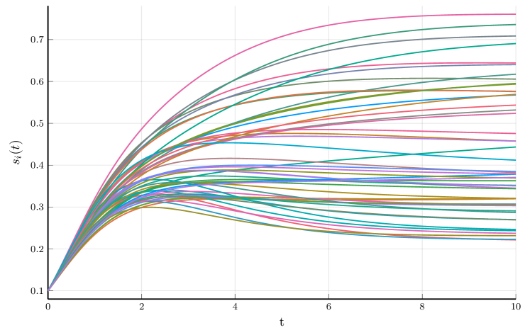
Figure 1: Set of individual trajectories $t\in[0;10]\mapsto s_{1:N}(t)$ obtained with Julia package DifferentialEquations.jl for a population of size $N=50$.

Figure 1 represents the evolution of a population of size $N=50$ individuals over the time interval $[0;10]$ for a given initial configuration. We can notice by looking at the final slopes of the growth curves that the sizes of the different plants have, for a vast majority, reached stationary sizes at time $T=10$, leading to think that the whole population may have a stationary distribution.

3 Mean-field model

We study the asymptotic behavior of the system (5) when the size $N$ of the population tends towards $+\infty$. More precisely, we would like to characterize the growth of an individual plant in an infinitely crowded population. This evolution is represented by the notion of characteristic flow, which drives the individual and the global dynamics at the same time. Qualitatively, the characteristic flow can be seen as the growth of a plant in interaction with a population represented by a probability distribution, instead of a list of individuals like in the case of the differential system (5). We first introduce the notion of population empirical measure and empirical flow.

3.1 Population empirical measure and empirical flow

Definition 1.

Let $z^{0}_{1:N}=(s_{i}^{0},x_{i},S_{i},\gamma_{i})_{1\leq i\leq N}\in\mathcal{Z}^{N}$ be an initial configuration satisfying the same assumptions as in proposition 1. Let $t\in\mathbb{R}_{+}\mapsto(s_{i}(t))_{1\leq i\leq N}\in(\mathbb{R}_{+}^{*})^{N}$ be the solution of the system (5). We define as the population empirical measure the trajectory taking values in the space $\mathcal{P}(\mathcal{Z})$ of probability measures over $\mathcal{Z}$:

$$t\in\mathbb{R}_{+}\mapsto\hat{\mu}_{N}(t,z_{1:N}^{0})\in\mathcal{P}(\mathcal{Z})$$ (12)

where for all $t\geq 0$,

$$\hat{\mu}_{N}(t,z_{1:N}^{0})(dz)=\frac{1}{N}\sum_{i=1}^{N}\delta(s_{i}(t),x_{i},S_{i},\gamma_{i})(dz)$$ (13)

where $\delta(s_{i}(t),x_{i},S_{i},\gamma_{i})$ is the Dirac distribution centered at the point $(s_{i}(t),x_{i},S_{i},\gamma_{i})$.

The population empirical measure can be understood as a uniform distribution over the individuals in the population. The dynamics of the population empirical measure can be characterized by a function related to the semi-group of the differential system (5), that we refer to as the empirical flow, denoted by $\hat{s}_{N}$. The property characterizing the empirical flow can be written as follows: for all $t\geq 0$,

$$\hat{\mu}_{N}(t,z^{0}_{1:N})(ds,d\theta)=(\hat{s}_{N}(t,s,\theta),\theta)\#\hat{\mu}(0,z^{0}_{1:N})(ds,d\theta)$$ (14)

For any function $f:\mathcal{X}\rightarrow\mathcal{Y}$ and any probability measure $\mu\in\mathcal{P}(\mathcal{X})$, the operator $f(x)\#\mu(dx)\in\mathcal{P}(\mathcal{Y})$ is the pushforward measure of $\mu$ by the function $f$, defined for all bounded and measurable function $\varphi:\mathcal{Y}\rightarrow\mathbb{R}$ by

$$\int_{\mathcal{Y}}\varphi(y)[f(x)\#\mu(dx)](dy)=\int_{\mathcal{X}}\varphi(f(x))\mu(dx)$$ (15)

The next proposition gives the expression of the empirical flow $\hat{s}_{N}$.

Proposition 2.

Let $(s_{i}^{0},\theta_{i})_{1\leq i\leq N}\in\mathcal{Z}^{N}$ be an initial configuration of the population satisfying the same assumptions as in proposition 1. Then for all $(s^{0},x,S,\gamma)\in\mathcal{Z}$ such that $s_{m}<s^{0}<S$ and $s_{m}<S<s_{m}e^{R_{M}}$, the differential equation

$$\left\{\begin{array}[]{l}s(0)=s^{0}\\ \displaystyle\forall t\geq 0,\frac{ds}{dt}(t)=\gamma s(t)\left[\log\left(\frac{S}{s_{m}}\right)\left(1-\hat{C}_{N}(s(t),x,\hat{\mu}_{N}(t,z^{0}_{1:N}))\right)-\log\left(\frac{s(t)}{s_{m}}\right)\right]\end{array}\right.$$ (16)

where

$$\hat{C}_{N}(s(t),x,\hat{\mu}_{N}(t,z^{0}_{1:N}))\!=\!\frac{N}{N-1}\!\int_{\mathbb{R}_{+}^{*}\times\mathbb{R}^{2}}\!\!\!\!\!\!\!\!\!C(s(t),s^{\prime},|x-x^{\prime}|)\hat{\mu}_{N}^{s,x}(t,z^{0}_{1:N})(ds^{\prime},dx^{\prime})-\frac{C(s(t),s(t),0)}{N-1}$$

has a unique solution, which is defined over $\mathbb{R}_{+}$. In equation (16), we use the notation $\hat{\mu}_{N}^{s,x}(t,z^{0}_{1:N})$ for the marginal distribution of $\hat{\mu}_{N}(t,z^{0}_{1:N})$ with respect to the variables $s,x$. We call empirical flow the function associating the initial condition to the solution of the differential equation and we denote:

$$(t,s^{0},\theta)\in\mathbb{R}_{+}\times\mathcal{Z}\mapsto\hat{s}_{N}(t,s^{0},\theta,z^{0}_{1:N})\in\mathbb{R}_{+}^{*}.$$ (17)

Proof.

: We only need to prove that the maximal solution of the equation is bounded over its definition interval, which will imply that the maximal solution is global. We have, for all $t$ in the definition interval, the following inequalities on the competition term.

$$-\frac{\log\left(\frac{s(t)}{s_{m}}\right)}{2R_{M}(N-1)}\leq\hat{C}_{N}(s(t),x,\hat{\mu}_{N}(t))\leq\frac{N}{N-1}-\frac{\log\left(\frac{s(t)}{s_{m}}\right)}{2R_{M}(N-1)}$$ (18)

By implying lemma 4, we can obtain bounds on the solution $t\mapsto s(t)$.

$$s_{m}\exp\left(-\frac{2R_{M}}{2N-3}\right)\leq s(t)\leq s_{m}\exp\left(\frac{6N-5}{2N-3}R_{M}\right)$$ (19)

∎

The empirical flow is such that $\forall i\in\llbracket 1;N\rrbracket,~{}\hat{s}_{N}(t,s_{i}^{0},\theta_{i},z^{0}_{1:N})=s_{i}(t)$ and therefore we have $(\hat{s}_{N}(t,s^{0},\theta,z^{0}_{1:N}),\theta)\#\hat{\mu}_{N}(0,z^{0}_{1:N})(ds^{0},d\theta)=\hat{\mu}_{N}(t,z^{0}_{1:N})(ds_{t},d\theta)$.

Let us assume that the initial population empirical measure $\hat{\mu}_{N}(0,z^{0}_{1:N})$ has a limit when $N\rightarrow\infty$ for some metric. This is the case, for instance, if the initial configuration of the population is composed by independent samples drawn from some distribution $\mu_{0}$, which is the illustration we used for the simulation in Section 2.4.2. In this case, we have indeed that

$$\hat{\mu}_{N}(0,z^{0}_{1:N})\xrightarrow[N\rightarrow\infty]{\mathcal{D}}\mu_{0}$$ (20)

in distribution $\mu_{0}$-almost surely.

The differential equation characterizing the empirical flow can be rewritten as follows:

$$\frac{\partial\hat{s}_{N}}{\partial t}(t,s^{0},\theta,z^{0}_{1:N})=\gamma\hat{s}_{N}(t,s^{0},\theta,z^{0}_{1:N})\left(\log\left(\frac{S}{s_{m}}\right)\right.$$ (21)

$$\times\left(1-\frac{N}{N-1}\int_{\mathcal{Z}}C(\hat{s}_{N}(t,s^{0},\theta,z^{0}_{1:N}),\hat{s}_{N}(t,s^{\prime},\theta^{\prime},z^{0}_{1:N}),|x-x^{\prime}|)\hat{\mu}_{N}(0,z^{0}_{1:N})(ds^{\prime},d\theta^{\prime})\right.$$

$$\left.\left.+\frac{C(\hat{s}_{N}(t,s^{0},\theta,z^{0}_{1:N}),\hat{s}_{N}(t,s^{0},\theta,z^{0}_{1:N}),0)}{N-1}\right)-\log\left(\frac{\hat{s}_{N}(t,s^{0},\theta,z^{0}_{1:N})}{s_{m}}\right)\right)$$

From this expression, we can postulate that if the empirical flow $\hat{s}_{N}$ has a limit $s_{\infty}$ in some sense when the size of the population tends to infinity, then this limit must satisfy the following equation:

$$\frac{\partial s_{\infty}}{\partial t}(t,s^{0},\theta)=\gamma s_{\infty}(t,s^{0},\theta)\left(\log\left(\frac{S}{s_{m}}\right)\left(1-\int_{\mathcal{Z}}C(s_{\infty}(t,s^{0},\theta),s_{\infty}(t,s^{\prime},\theta^{\prime}),|x-x^{\prime}|)\mu_{0}(ds^{\prime},d\theta^{\prime})\right)\right.$$ (22)

$$\left.-\log\left(\frac{s_{\infty}(t,s^{0},\theta)}{s_{m}}\right)\right)$$

The objectives of the next sections is to prove that the object $s_{\infty}$ exists and is uniquely defined, and that the convergence of $\hat{s}_{N}$ towards $s_{\infty}$ holds for some specific metric.

3.2 Existence and uniqueness of the mean-field flow

The equations of the type (22) characterizes the mean-field flow $s_{\infty}(t)$, in reference to the mean-field distribution $\mu_{\infty}(t)$, representing the propagation through time of the initial datum $\mu_{0}$ by the dynamics of an infinitely-crowded population. The literature studying this type of integro-differential equations is vast. In our case, we were mainly inspired by the work of Golse [13] and Bolley et al. [5], who have studied dynamics that share similar properities with system (5).

Theorem 1.

Let $\Theta=\mathbb{R}^{2}\times[s_{m};s_{m}e^{R_{M}}]\times[0;\gamma_{M}]$ where $\gamma_{M}>0$. Let $\mu_{0}\in\mathcal{P}(\mathbb{R}_{+}^{*}\times\Theta)$ such that

$$\int_{\mathbb{R}_{+}^{*}}\log\left(\frac{s}{s_{m}}\right)^{2}\mu_{0}^{s}(ds)<+\infty$$

Then there exists a unique function $s_{\infty}:(t,s_{0},\theta)\in\mathbb{R}_{+}\times\mathbb{R}_{+}^{*}\times\Theta\mapsto s_{\infty}(t,s_{0},\theta)\in\mathbb{R}_{+}^{*}$ continuously differentiable with respect to $t$, such that for all $(s_{0},\theta)\in\mathbb{R}_{+}^{*}\times\Theta$, we have

$$\left\{\begin{array}[]{l}s_{\infty}(0,s_{0},\theta)=s_{0}\\ \displaystyle\frac{\partial s_{\infty}}{\partial t}(t,s_{0},\theta)=\gamma s_{\infty}(t,s_{0},\theta)\left(\log\left(\frac{S}{s_{m}}\right)\left(1-\mathcal{C}(s_{\infty},t,s_{0},\theta)\right)-\log\left(\frac{s_{\infty}(t,s_{0},\theta)}{s_{m}}\right)\right)\end{array}\right.$$ (23)

$$\text{where }\mathcal{C}(s_{\infty},t,s_{0},\theta)=\int_{\mathbb{R}_{+}^{*}\times\Theta}C(s_{\infty}(t,s_{0},\theta),s_{\infty}(t,s_{0}^{\prime},\theta^{\prime}),|x-x^{\prime}|)\mu_{0}(ds_{0}^{\prime},d\theta^{\prime})$$

Proof.

For convenience, we study the equation satisfied by the logarithm of the size instead, i.e., $\displaystyle r_{\infty}(t)=\log\left(\frac{s_{\infty}(t)}{s_{m}}\right)$, and $\displaystyle\nu_{0}(dr,d\theta)=\left(\log\left(\frac{s}{s_{m}}\right),\theta\right)\#\mu_{0}(ds,d\theta)$.

$$\left\{\begin{array}[]{l}\displaystyle\frac{\partial r_{\infty}}{\partial t}(t,r_{0},\theta)=\gamma\left(\log\left(\frac{S}{s_{m}}\right)\left(1-\mathcal{C}_{r}(r_{\infty},t,r_{0},\theta)\right)-r_{\infty}(t,r_{0},\theta)\right)\\ r(t_{0},r_{0},\theta)=r_{0}\end{array}\right.$$ (24)

$$\text{where }\mathcal{C}_{r}(r_{\infty},t,r_{0},\theta)=\int_{\mathbb{R}\times\Theta}C_{r}(r_{\infty}(t,r_{0},\theta),r_{\infty}(t,r_{0}^{\prime},\theta^{\prime}),|\theta_{x}-\theta^{\prime}_{x}|)\nu_{0}(dr_{0}^{\prime},d\theta^{\prime})$$

$$\text{and }C_{r}(r,r^{\prime},|x-x^{\prime}|)=\frac{r^{\prime}}{2R_{M}\left(1+\frac{|x-x^{\prime}|^{2}}{\sigma_{x}^{2}}\right)}\left(1+\tanh\left(\frac{r^{\prime}-r}{\sigma_{r}}\right)\right)$$

The above equation is equivalent to the following integral form:

$$r_{\infty}(t,r_{0},\theta)=r_{0}+\gamma\int_{t_{0}}^{t}\left(\log\left(\frac{S}{s_{m}}\right)(1-\mathcal{C}_{r}(r_{\infty},\tau,r_{0},\theta))-r_{\infty}(\tau,r_{0},\theta)\right)d\tau$$ (25)

The outline of the proof is as follows:

1. we show that equation (25) admits a solution in a specific space of continuous functions defined over a small time interval $[t_{0}-\delta t;t_{0}+\delta t]$.

2. We derive upper-bounds of the solution with respect to spatial and time variables.

3. We show that the solution of (25) is uniquely defined over its definition interval

4. A semi-group structure is proved for the solutions of (25).

5. We prove that $\mathbb{R}_{+}$ is included in the definition interval of the maximal solution associated with the initial data $(0,\nu_{0})$.

Local existence

Let $t_{0}\in\mathbb{R}$, $r^{*}>0$, $\delta t>0$. Let us define the following function over the space of continuous functions over $[t_{0}-\delta t;t_{0}+\delta t]\times\mathbb{R}\times\Theta$:

$$\rho\in\mathcal{C}^{0}([t_{0}-\delta t;t_{0}+\delta t] \times\mathbb{R}\times\Theta\rightarrow\mathbb{R})$$

$$\longmapsto\|\rho\|_{t_{0},\delta t}=\sup\left\{\frac{|\rho(t,r,\theta)|}{r^{*}+|r|},(t,r,\theta)\in[t_{0}-\delta t;t_{0}+\delta t]\times\mathbb{R}\times\Theta\right\}\in\bar{\mathbb{R}}$$

The space of continuous functions $\mathcal{SL}_{t_{0},\delta t}=\left\{\rho\in\mathcal{C}^{0}([t_{0}-\delta t;t_{0}+\delta t]\times\mathbb{R}\times\Theta\rightarrow\mathbb{R})|~{}\|\rho\|_{t_{0},\delta t}<\infty\right\}$ is a Banach space for the norm $\rho\in\mathcal{SL}_{t_{0},\delta t}\mapsto\|\rho\|_{t_{0},\delta t}\in\mathbb{R}_{+}$. Over $\mathcal{SL}_{t_{0},\delta t}$, we define the functional:

$$(\rho,t,r_{0},\theta)\in\mathcal{SL}_{t_{0},\delta t}\times[t_{0}-\delta t;t_{0}+\delta t]\times\mathbb{R}\times\Theta$$ (26)

$$\longmapsto\Phi(\rho,t,r_{0},\theta)=r_{0}+\gamma\int_{t_{0}}^{t}\left(\log\left(\frac{S}{s_{m}}\right)(1-\mathcal{C}_{r}(\rho,\tau,r_{0},\theta))-\rho(\tau,r_{0},\theta)\right)d\tau$$

We have the following inequalities on the function $\Phi$, for $\rho_{1},\rho_{2}\in\mathcal{SL}_{t_{0},\delta t}$

$$\|\Phi(\rho_{1})\|_{t_{0},\delta t}\leq\max\left\{1+\gamma_{M}\delta t\|\rho_{1}\|_{t_{0},\delta t},\quad\gamma_{M}\delta t\frac{R_{M}+\|\rho\|_{t_{0},\delta t}(R_{1}(\nu_{0})+r^{*})}{r^{*}}\right\}$$

$$\|\Phi(\rho_{1})-\Phi(\rho_{2})\|_{t_{0},\delta t}\leq\gamma_{M}\delta t\|\rho_{1}-\rho_{2}\|_{t_{0},\delta t}\max\left\{1+\frac{\|\rho_{1}\|_{t_{0},\delta t}}{2R_{M}\sigma_{r}},\right.$$

$$\left.\frac{(2R_{M}\sigma_{r}+\|\rho_{1}\|_{t_{0},\delta t}R_{1}(\nu_{0}))r^{*}+4R_{1}(\nu_{0})R_{M}\sigma_{r}+R_{M}R_{2}(\nu_{0})(\|\rho_{1}\|_{t_{0},\delta t}+\|\rho_{2}\|_{t_{0},\delta t})}{2R_{M}\sigma_{r}r^{*}}\right\}$$

$$\text{with for }d\in\{1,2\},\quad R_{d}(\nu_{0})=\int_{\mathbb{R}}(r^{*}+|r|)^{d}\nu_{0}^{r}(dr)$$

Therefore, there exists $\delta t>0$ and $\rho_{m}>1$ such that

• for all $\rho\in\mathcal{SL}_{t_{0},\delta t}$ satisfying $\|\rho\|_{t_{0},\delta t}\leq\rho_{m}$ we have $\|\Phi(\rho)\|_{t_{0},\delta t}\leq\rho_{m}$;

• $\Phi$ is a contraction over the ball $\mathcal{B}_{t_{0},\delta t,\rho_{m}}=\{\rho\in\mathcal{SL}_{t_{0},\delta t}|~{}\|\rho\|_{t_{0},\delta t}\leq\rho_{m}\}$.

By Banach fixed-point theorem, the map $\Phi$ has a unique fixed-point $r_{\infty}\in\mathcal{B}_{t_{0},\delta t,\rho_{m}}$. Therefore, for all $t_{0}\in\mathbb{R}$ and $\nu_{0}\in\mathcal{P}_{2}(\mathbb{R}\times\Theta)$, there exists an interval $\mathcal{I}$ containing $t_{0}$ and a function $r_{\infty}(t_{0},\nu_{0})$ satisfying the equation (25) for all $(t,r_{0},\theta)\in\mathcal{I}\times\mathbb{R}\times\Theta$.

Propagation of the moment of the initial distribution

Let $(r_{\mathcal{I}},\mathcal{I})$ a solution of the equation (25) over an interval $\mathcal{I}$ containing $t_{0}$. Then let us prove that for all $t\in\mathcal{I}$,

$$\|r_{\mathcal{I}}(t)\|=\sup\left\{\frac{|r_{\mathcal{I}}(t,r_{0},\theta)|}{r^{*}+|r_{0}|},(r_{0},\theta)\in\mathbb{R}\times\Theta\right\}<+\infty$$ (27)

We have the following inequality on the flow $r_{\mathcal{I}}$ for all $t\in\mathcal{I}$ such that for all $t\geq t_{0}$, $r\in\mathbb{R}$, $\theta\in$ $\Theta$:

$$|r_{\mathcal{I}}(t,r_{0},\theta)|\leq|r_{0}|+\gamma\int_{t_{0}}^{t}\left[\log\left(\frac{S}{s_{m}}\right)\left(1+\int_{\mathbb{R}\times\Theta}\frac{|r_{\mathcal{I}}(\tau,r_{0}^{\prime},\theta^{\prime})|}{R_{M}}\nu_{0}(dr_{0}^{\prime},d\theta^{\prime})\right)+|r_{\mathcal{I}}(\tau,r_{0},\theta)|\right]d\tau$$ (28)

We therefore need to upper-bound the first-order moment.

$$\int_{\mathbb{R}\times\Theta}|r_{\mathcal{I}}(t,r_{0},\theta)|\nu_{0}(dr_{0},d\theta)\leq\int_{\mathbb{R}}|r_{0}|\nu_{0}^{r}(dr_{0})+(t-t_{0})\int_{[s_{m};s_{m}e^{R_{M}}]\times[0;\gamma_{M}]}\!\!\!\!\!\!\!\!\!\!\!\!\!\!\!\!\!\!\!\!\!\!\!\!\!\!\!\!\!\!\!\!\!\!\gamma\log\left(S/s_{m}\right)\nu_{0}^{S,\gamma}(dS,d\gamma)$$ (29)

$$+2\gamma_{M}\int_{t_{0}}^{t}\int_{\mathbb{R}\times\Theta}|r_{\mathcal{I}}(\tau,r_{0},\theta)|\nu_{0}(dr_{0},d\theta)d\tau$$

By Grönwall lemma, there exists $\bar{R}>0$, a constant not depending on $r_{0}$ and $t$, such that

$$\int_{\mathbb{R}\times\Theta}|r_{\mathcal{I}}(t,r_{0},\theta)|\nu_{0}(dr_{0},d\theta)\leq\left(\int_{\mathbb{R}}|r_{0}|\nu_{0}^{r}(dr_{0})+\bar{R}\right)e^{2\gamma_{M}(t-t_{0})}-\bar{R}$$ (30)

By applying Grönwall lemma a second time on $|r_{\mathcal{I}}(t,r_{0},\theta)|$, we obtain that there exists constants $\bar{r}_{1},\bar{r}_{2},\bar{r}_{3}>0$ such that, for all $t\in\mathcal{I}\cap[t_{0};+\infty),r_{0}\in\mathbb{R},\theta\in\Theta$,

$$|r_{\mathcal{I}}(t,r_{0},\theta)|\leq(|r_{0}|+\bar{r}_{1})e^{\gamma_{M}(t-t_{0})}+\bar{r}_{2}e^{2\gamma_{M}(t-t_{0})}+\bar{r}_{3}$$ (31)

So $\|r_{\mathcal{I}}(t)\|<+\infty$. We apply the same reasoning to extend this inequality for all $t\in\mathcal{I}\cap(-\infty;t_{0}]$. In particular, we have, for all $t\in\mathcal{I}$,

$$\int_{\mathbb{R}\times\Theta}|r_{\mathcal{I}}(t,r_{0},\theta)|^{2}\nu_{0}(dr_{0},d\theta)<\infty$$ (32)

Local uniqueness

We consider the function on the space of continous functions

$$\rho\in\mathcal{C}^{0}(\mathbb{R}\times\Theta\rightarrow\mathbb{R})\longmapsto\|\rho\|=\sup\left\{\frac{|\rho(r,\theta)|}{r^{*}+|r|},(r,\theta)\in\mathbb{R}\times\Theta\right\}$$ (33)

which is a norm over the Banach space $\mathcal{SL}=\{\rho\in\mathcal{C}^{0}(\mathbb{R}\times\Theta\rightarrow\mathbb{R})|~{}\|\rho\|<+\infty\}$. Let $(r_{\mathcal{I}},\mathcal{I})$ and $(r_{\mathcal{J}},\mathcal{J})$ be two solutions of the equation (25) on the the intervals $\mathcal{I}$ and $\mathcal{J}$ respectively, associated with the same initial data $(t_{0},\nu_{0})$, with $t_{0}\in\mathcal{I}\cap\mathcal{J}=\mathcal{J}\subset\mathcal{I}$. Then we can prove that the restriction $r_{\mathcal{I}|\mathcal{J}}$ of $r_{\mathcal{I}}$ is equal to $r_{\mathcal{J}}$. Let us consider the interval $\mathcal{J}^{\prime}=\{t\in\mathcal{J}|t\geq t_{0},\forall\tau\in[t_{0};t],~{}r_{\mathcal{I}}(\tau)=r_{\mathcal{J}}(\tau)\}$ and let $t^{*}=\sup\mathcal{J}^{\prime}$. Then $t^{*}\geq\delta t>0$ by uniqueness of the fixed point of the map $\Phi$ previously defined. If $t^{*}<\sup\mathcal{J}$, then $t^{*}$ is finite, and we obtain by continuity of the norm $\|\cdot\|$ that $r_{\mathcal{I}}(t^{*})=r_{\mathcal{J}}(t^{*})$. Then for any $\delta t^{*}>0$ such that $t^{*}+\delta t^{*}\in\mathcal{J}$, there exists $K(t^{*},\delta t^{*})>0$ verifying for all $t\in[t^{*};t^{*}+\delta t^{*}]$

$$\|r_{\mathcal{I}}(t)-r_{\mathcal{J}}(t)\|\leq K(t^{*},\delta t^{*})\int_{t^{*}}^{t}\|r_{\mathcal{I}}(\tau)-r_{\mathcal{J}}(\tau)\|d\tau$$

It follows that $r_{\mathcal{I}}(t)=r_{\mathcal{J}}(t)$ for all $t\in[t^{*};t^{*}+\delta t^{*}]$, which is in contradiction with the definition of $t^{*}$. As a consequence, $t^{*}=\sup\mathcal{J}$. We use the same reasoning to prove that

$$\inf\{t\in\mathcal{J}|\forall\tau\in[t;t_{0}],~{}r_{\mathcal{I}}(\tau)=r_{\mathcal{J}}(\tau)\}=\inf\mathcal{J}$$ (34)

The local existence and uniqueness implies the existence and uniqueness of the maximal solution for equation (25) for any initial data $(t_{0},\nu_{0})$. This means that there exists a solution and an interval $(r_{\mathcal{I}},\mathcal{I})$ such that for all $(r_{\mathcal{J}},\mathcal{J})$ associated with the same initial data, we have $\mathcal{J}\subset\mathcal{I}$.

Semi-group structure of the flow

Let $(r_{\mathcal{I}}(t_{0},\nu_{0}),\mathcal{I})$ be the maximal solution of the equation (25) associated with the initial data $(t_{0},\nu_{0})$. We use the following notation:

$$r_{\mathcal{I}}(t_{0},\nu_{0}):(t,r,\theta)\in\mathcal{I}\times\mathbb{R}\times\Theta\mapsto r_{\mathcal{I}}(t,r,\theta;t_{0},\nu_{0})\in\mathbb{R}$$ (35)

Let $t_{1}\in\mathcal{I}$ and let $r_{\mathcal{I}}(t_{1},\nu_{t_{1}})$ be the maximal solution associated with $(t_{1},\nu_{t_{1}})$ where $\nu_{t_{1}}(dr_{1},d\theta)=(r_{\mathcal{I}}(t_{1},r_{0},\theta;t_{0},\nu_{0}),\theta)\#\nu_{0}(dr_{0},d\theta)$ is defined as the pushforward measure from $t_{0}$ to $t_{1}$ by the flow. Then, by uniqueness of the maximal solution, it follows that for all $t\in\mathcal{I}$, $r_{0}\in\mathbb{R}$, $\theta\in\Theta$

$$r_{\mathcal{I}}(t,r_{0},\theta;t_{0},\nu_{0})=r_{\mathcal{I}}(t,r_{\mathcal{I}}(t_{1},r_{0},\theta;t_{0},\nu_{0}),\theta;t_{1},\nu_{t_{1}})$$ (36)

Globality of the maximal solution

Let $(r_{\mathcal{I}}(0,\nu_{0}),\mathcal{I})$ be the maximal solution associated with $(0,\nu_{0})$. Then let us prove that $\mathbb{R}_{+}\subset\mathcal{I}$. Let $t^{*}=\sup\mathcal{I}$. If $t^{*}<+\infty$, then $t^{*}$ cannot be in $\mathcal{I}$ as it would contradict the maximality of the solution $(r_{\mathcal{I}},\mathcal{I})$. But even if $t^{*}\notin\mathcal{I}$, we still obtain a contradiction with the maximality of the solution by considering the solution associated with the initial data $(t^{*},\nu_{t^{*}})$ where

$$\nu_{t^{*}}=(\tilde{r}_{\mathcal{I}}(t^{*},\cdot,\cdot),\mathrm{Id}_{\Theta})\#\nu_{0}$$ (37)

$$\text{with }\tilde{r}_{\mathcal{I}}(t^{*},r_{0},\theta)=r_{0}+\int_{0}^{t^{*}}\frac{\partial r_{\mathcal{I}}}{\partial t}(t,r_{0},\theta;0,\nu_{0})dt$$

The above integral is absolutely convergent thanks to the upper-bound (31).

Conclusion

By making the reverse change of variable $\displaystyle s_{\infty}=s_{m}e^{r_{\infty}}$, we conclude that there exists a unique function $s_{\infty}$ defined over $\mathbb{R}_{+}$ satisfying the equation (23). ∎

We define the mean-field distribution of the population as the pushforward measure of the initial distribution $\mu_{0}$ by the mean-field flow.

$$\forall t\geq 0,\quad\mu_{\infty}(t)(ds_{t},d\theta)=(s_{\infty}(t,s_{0},\theta),\theta)\#\mu_{0}(ds_{0},d\theta)$$ (38)

Using equation (23), we can prove that the distribution $\mu_{\infty}$ is the unique solution in the sense of the distribution of the following partial differential equation:

$$\left\{\begin{array}[]{ll}\displaystyle\frac{\partial\mu_{\infty}}{\partial t}(t,ds,d\theta)+\frac{\partial}{\partial s}\left[\gamma s\left(\log\left(\frac{S}{s_{m}}\right)\left(1-\int_{\mathbb{R}_{+}^{*}\times\mathbb{R}^{2}}\!\!\!\!\!\!\!\!\!\!\!\!C(s,s^{\prime},|x-x^{\prime}|\mu^{s,x}_{\infty}(t,ds^{\prime},dx^{\prime})\right)\right)\mu_{\infty}(t,ds,d\theta)\right]=0\\ \mu_{\infty}(0,ds,d\theta)=\mu_{0}(ds,d\theta)\end{array}\right.$$ (39)

Conversely, the distribution of the random variable $s_{\infty}(t,s_{0},\theta)$, with $(s_{0},\theta)$ being distributed according to $\mu_{0}$, is the marginal $\mu_{\infty}^{s}(t)$. In the next section, we prove the convergence of $\hat{\mu}_{N}(t,z^{0}_{1:N})$ towards $\mu_{\infty}(t)$, which proves in the same time the convergence of $\hat{s}_{N}(t,s_{0},\theta,z^{0}_{1:N})$ towards $s_{\infty}(t,s_{0},\theta)$ when $N\rightarrow+\infty$.

3.3 Convergence of the empirical flow towards the mean-field flow

We establish in this section that the population empirical measure $\hat{\mu}_{N}(t,z^{0}_{1:N})$ converges almost surely towards $\mu_{\infty}(t)$ for the Wasserstein metric $\mathcal{W}_{p}$, which is defined (Villani [24]), for any distributions $\mu_{1},\mu_{2}\in\mathcal{P}(\mathcal{Z})$, as

$$\mathcal{W}_{p}(\mu_{1},\mu_{2})^{p}=\inf\left\{\iint_{\mathcal{Z}^{2}}m_{\mathcal{Z}}(z_{1},z_{2})^{p}\pi(dz_{1},dz_{2}),\quad\pi\in\Pi(\mu_{1},\mu_{2})\right\}$$ (40)

where $m_{\mathcal{Z}}$ is a metric defined over the space $\mathcal{Z}$ and $\Pi(\mu_{1},\mu_{2})$ is the set of couplings between the distributions $\mu_{1},\mu_{2}$, i.e.,

$$\Pi(\mu_{1},\mu_{2})=\left\{\pi(dz_{1},dz_{2})\in\mathcal{P}(\mathcal{Z}^{2})|~{}\pi^{z_{1}}(dz_{1})=\mu_{1}(dz_{1})\text{ and }\pi^{z_{2}}(dz_{2})=\mu_{2}(dz_{2})\right\}$$ (41)

The convergence of $\hat{\mu}_{N}0,z^{0}_{1:N})\rightarrow\mu_{0}$ is propagated to any time using the argument refered to in the literature as Dobrushin’s stability [11].

Theorem 2.

Let $\mu_{0}\in\mathcal{P}(\mathbb{R}_{+}*\times\Theta)$ such that $\displaystyle\int_{\mathbb{R}^{2}}|x|^{2}\mu_{0}^{x}(dx)<+\infty$ and such that there exists $s_{0}^{\min},s_{0}^{\max},S_{m}$ satisfying

$$s_{m}<s_{0}^{\min}<s_{0}^{\max}<S_{m}<s_{m}e^{R_{M}}$$ (42)

$$\mathbb{P}\left\{s_{0}\sim\mu_{0}^{s}|s_{0}^{\min}<s_{0}<s_{0}^{\max}\right\}=1$$

$$\mathbb{P}\left\{S\sim\mu_{0}^{S}|S_{m}<S<s_{m}e^{R_{M}}\right\}=1$$

We consider a sequence $(s_{n}^{0},x_{n},S_{n},\gamma_{n})_{n\in\mathbb{N}^{*}}$ of independant and identically distributed sample of the initial distribution $\mu_{0}$. We build from this sequence the sequence of empirical measures $(\hat{\mu}_{N})_{N\in\mathbb{N}^{*}}$ defined for all $N\geq 1$ by equation (13). Then we have the following almost sure convergence:

$$\mathbb{P}\left\{(s_{n}^{0},x_{n},S_{n},\gamma_{n})_{n\in\mathbb{N}^{*}}\sim\mu_{0}^{\otimes\infty}|\forall t\geq 0,~{}\lim_{N\rightarrow\infty}\mathcal{W}_{1}\left(\hat{\mu}_{N}(t),\mu_{\infty}(t)\right)=0\right\}=1$$ (43)

Proof.

Let $z_{1:N}^{0}\in([s_{0}^{\min};s_{0}^{\max}]\times\Theta)^{N}$ be an initial configuration. Let $\pi_{s}\in\Pi\left(\hat{\mu}^{s}_{N}(0,z^{0}_{1:N}),\mu_{0}^{s}\right)$, $\pi_{x}\in\Pi\left(\hat{\mu}_{N}^{x}(0,z^{0}_{1:N}),\mu_{0}^{x}\right)$, $\pi_{S}\in\Pi\left(\hat{\mu}_{N}^{S}(0,z^{0}_{1:N}),\mu_{0}^{S}\right)$ and $\pi_{\gamma}\in\Pi\left(\hat{\mu}_{N}^{\gamma}(0,z^{0}_{1:N}),\mu_{0}^{\gamma}\right)$ be a set of couplings associated with the marginal distributions of the empirical distribution and the initial distribution. From these couplings, we build the initial coupling $\pi_{0}=\pi_{s}\otimes\pi_{x}\otimes\pi_{S}\otimes\pi_{\gamma}$, which is in $\Pi\left(\hat{\mu}_{N}(0,z^{0}_{1:N}),\mu_{0}\right)$.

We consider the empirical flow $\hat{s}_{N}$ associated with the empirical population measure $t\mapsto\hat{\mu}_{N}(t,z^{0}_{1:N})$. For any $t\geq 0$, we define the coupling

$$\pi_{t}(d\hat{s}_{t},d\theta_{1},ds_{t},d\theta_{2}) =(\hat{s}_{N}(t,\hat{s}_{0},\theta_{1},z^{0}_{1:N}),\theta_{1},s_{\infty}(t,s_{0},\theta_{2}),\theta_{2})\#\pi_{0}(d\hat{s}_{0},d\theta_{1},ds_{0},d\theta_{2})$$ (44)

$$\in\Pi\left(\hat{\mu}_{N}(t,z^{0}_{1:N}),\mu_{\infty}(t)\right)$$

The space $\mathbb{R}_{+}^{*}\times\Theta$ is endowed with the metric $m_{\mathcal{Z}}$ defined by

$$m_{\mathcal{Z}}(s_{1},\theta_{1},s_{2},\theta_{2})=\frac{|s_{1}-s_{2}|+|S_{1}-S_{2}|}{s_{m}}+\frac{|x_{1}-x_{2}|}{\ell}+\tau_{r}|\gamma_{1}-\gamma_{2}|$$ (45)

$$=\frac{|s_{1}-s_{2}|}{s_{m}}+m_{\Theta}(\theta_{1},\theta_{2})$$

where $\ell,\tau_{r}>0$ are arbitrary constants. For this metric and for any time $t\geq 0$, the Wasserstein distance between distributions $\hat{\mu}_{N}(t,z^{0}_{1:N})$ and $\mu(t)$ is expressed as follows

$$\mathcal{W}_{1}(\hat{\mu}_{N}(t,z^{0}_{1:N}),\mu(t))=\inf \left\{\iint_{(\mathbb{R}_{+}^{*}\times\Theta)^{2}}\!\!\!\!\!\!\!\!\!\!\!\!\!m_{\mathcal{Z}}(s_{1},\theta_{1},s_{2},\theta_{2})\pi(ds_{1},d\theta_{1},ds_{2},d\theta_{2}),\right.$$ (46)

$$\left.\phantom{\int}\pi\in\Pi\left(\hat{\mu}_{N}(t,z^{0}_{1:N}),\mu(t)\right)\right\}$$

The coupling $\pi_{t}$ provides an upper-bound of the Wasserstein distance at time $t$.

$$\mathcal{W}_{1}(\mu_{N}(t,z_{1:N}^{0}),\mu(t))\leq\iint_{(\mathcal{\mathbb{R}}_{+}^{*}\times\Theta)^{2}}\left(\frac{|s_{1}-s_{2}|}{s_{m}}+m_{\Theta}(\theta_{1},\theta_{2})\right)\pi_{t}(ds_{1},d\theta_{1},ds_{2},d\theta_{2})$$ (47)

$$\leq\frac{1}{s_{m}}\iint_{(\mathbb{R}_{+}^{*}\times\Theta)^{2}}\!\!\!\!\!\!\!\!\!\!\!\!\!|\hat{s}_{N}(t,s_{1},\theta_{1})-s_{\infty}(t,s_{2},\theta_{2})|\pi_{0}(ds_{1},d\theta_{1},ds_{2},d\theta_{2})$$

$$+\iint_{\Theta^{2}}m_{\Theta}(\theta_{1},\theta_{2})\pi_{0}^{\theta}(d\theta_{1},d\theta_{2})$$

Let us focus on the first term of the upper-bound.

$$D^{\pi_{0}}_{N}(t)=\iint_{(\mathbb{R}_{+}^{*}\times\Theta)^{2}}\!\!\!\!\!\!\!\!\!\!\!\!\!\!\!\!|\hat{s}_{N}(t,s_{1},\theta_{1})-s_{\infty}(t,s_{2},\theta_{2})|\pi_{0}(ds_{1},d\theta_{1},ds_{2},d\theta_{2})$$ (48)

As detailed in the appendix, section A.1, we can prove that

$$D^{\pi_{0}}_{N}(t)\leq\frac{s_{0}^{\max}e^{R_{M}}R_{M}}{N-1}+\frac{tA(\hat{\mu}_{N}(0,z^{0}_{1:N}))}{N-1}+e^{R_{M}}\iint_{(\mathbb{R}_{+}^{*})^{2}}|s_{1}-s_{2}|\pi_{0}^{s}(ds_{1},ds_{2})$$ (49)

$$+tB(\hat{\mu}_{N}^{x}(0,z^{0}_{1:N}),\mu_{0}^{x})\sqrt{\iint_{\mathbb{R}^{4}}|x_{1}-x_{2}|^{2}\pi_{0}^{x}(dx_{1},dx_{2})}$$

$$+\alpha_{S}\iint_{[S_{m};s_{m}e^{R_{M}}]^{2}}|S_{1}-S_{2}|\pi_{0}^{S}(dS_{1},dS_{2})$$

$$+\alpha_{\gamma}t\iint_{[0;\gamma_{M}]^{2}}|\gamma_{1}-\gamma_{2}|\pi_{0}^{\gamma}(d\gamma_{1},d\gamma_{2})+\beta_{N}\int_{0}^{t}D^{\pi_{0}}_{N}(\tau)d\tau$$

where the functionals $A(\mu)$, $B(\mu_{1},\mu_{2})$ have the following expressions:

$$A(\mu)=\frac{1}{2R_{M}}\int_{\mathbb{R}_{+}^{*}\times[S_{m};s_{m}e^{R_{M}}]\times[0;\gamma_{M}]}\!\!\!\!\!\!\!\!\!\!\!\!\!\!\!\!\!\!\!\!\!\!\!\!\!\!\!\!\!\!\!\!\!\!\!\!\!\!\!\!\!\!\!\!\!\!\!\left(\gamma Ss/s_{m}\log(s/s_{m})+s_{0}^{\max}e^{R_{M}}R_{M}\gamma\log(S/s_{m})\right)\mu^{s,S,\gamma}(ds,dS,d\gamma)$$ (50)

$$B(\mu_{1},\mu_{2})=\frac{s_{0}^{\max}e^{R_{M}}R_{M}\gamma_{M}}{\sigma_{x}^{2}}\left(2\int_{\mathbb{R}^{2}}|x|\mu_{2}(dx)+\sqrt{2\int_{\mathbb{R}^{2}}|x|^{2}\mu_{2}(dx)+2\int_{\mathbb{R}^{2}}|x|^{2}\mu_{1}(dx)}\right.$$

$$\left.+\int_{\mathbb{R}^{2}}\sqrt{2\int_{\mathbb{R}^{2}}|x|^{2}\mu_{1}(dx)+2\int_{\mathbb{R}^{2}}|x|^{2}\mu_{1}(dx)-4x^{\prime}.\left(\int_{\mathbb{R}^{2}}x\mu_{1}(dx)+\int_{\mathbb{R}^{2}}x\mu_{2}(dx)\right)}\mu_{1}(dx^{\prime})\right)$$

and the coefficients $\alpha_{S},\alpha_{\gamma},\beta_{N}$ are

$$\alpha_{S}=(s^{0}_{\max}/S_{m})$$ (51)

$$\alpha_{\gamma}=s^{0}_{\max}\log\left(\frac{s_{0}^{\max}}{s_{m}}\right)e^{R_{M}}+s^{0}_{\max}e^{R_{M}}R_{M}$$

$$\beta_{N}=\frac{s_{0}^{\max}e^{R_{M}}R_{M}\gamma_{M}}{s_{m}^{N}\sigma_{r}}(1+\sigma_{r}/R_{M}+1/2)$$

We can find in the appendix, section A.1, the detailed derivation of the upper-bound of $D^{\pi_{0}}_{N}(t)$ in inequation (49). By Grönwall lemma, we obtain that

$$D^{\pi_{0}}_{N}(t)\leq\frac{1}{\beta_{N}}\left(\frac{A(\hat{\mu}_{N}(0,z^{0}_{1:N}))}{N-1}+B(\hat{\mu}_{N}^{x}(0,z^{0}_{1:N}),\mu_{0}^{x})\sqrt{\iint_{\mathbb{R}^{4}}|x_{1}-x_{2}|^{2}\pi_{0}^{x}(dx_{1},dx_{2})}\right.$$ (52)

$$\left.+\alpha_{\gamma}\iint_{[0;\gamma_{M}]^{2}}|\gamma_{1}-\gamma_{2}|\pi_{0}^{\gamma}(d\gamma_{1},d\gamma_{2})\right)\left(e^{\beta_{N}t}-1\right)+\left(\frac{s_{0}^{\max}e^{R_{M}}R_{M}}{N-1}\right.$$

$$+e^{R_{M}}\iint_{[s_{0}^{\min};s_{0}^{\max}]^{2}}|s_{1}-s_{2}|\pi_{0}^{s}(ds_{1},ds_{2})\left.+\alpha_{S}\iint_{[s_{m};s_{m}e^{R_{M}}]^{2}}|S_{1}-S_{2}|\pi_{0}^{S}(dS_{1},dS_{2})\right)e^{\beta_{N}t}$$

By gathering the terms from inequalities (52) and (47), we obtain the following upper-bound on the Wasserstein distance between the empirical distribution and the mean-field distribution at time $t$

$$\mathcal{W}_{1}(\hat{\mu}_{N}(t,z^{0}_{1:N}),\mu(t))\leq\frac{e^{R_{M}}}{s_{m}}\mathcal{W}_{1}(\hat{\mu}_{N}^{s}(0,z^{0}_{1:N}),\mu_{0}^{s})e^{\beta_{N}t}$$ (53)

$$+\left(\frac{B(\hat{\mu}_{N}^{x}(0,z^{0}_{1:N}),\mu_{0}^{x})}{s_{m}\beta_{N}}\left(e^{\beta_{N}t}-1\right)+\frac{1}{\ell}\right)\mathcal{W}_{2}(\hat{\mu}_{N}^{x}(0,z^{0}_{1:N}),\mu_{0}^{x}))$$

$$+\frac{\left(\alpha_{S}e^{\beta_{N}t}+1\right)}{s_{m}}\mathcal{W}_{1}(\hat{\mu}_{N}^{S}(0,z^{0}_{1:N}),\mu_{0}^{S})+\left(\frac{\alpha_{\gamma}}{s_{m}}\left(e^{\beta_{N}t}-1\right)+\tau_{r}\right)\mathcal{W}_{1}(\hat{\mu}_{N}^{\gamma}(0,z^{0}_{1:N}),\mu_{0}^{\gamma})$$

$$+\frac{1}{s_{m}(N-1)}\left(\frac{A_{N}(\hat{\mu}_{N}(0,z^{0}_{1:N}),\mu_{0})}{\beta_{N}}(e^{\beta_{N}t}-1)+s_{0}^{\max}e^{R_{M}+\beta_{N}t}R_{M}\right)$$

From the law of large numbers, we have the following almost sure convergences

$$\mathbb{P}(\Omega_{A})=\mathbb{P}\left\{z^{0}_{1:N}\sim\mu_{0}^{\otimes\infty}\mid\lim_{N\rightarrow\infty}A(\hat{\mu}_{N}(0,z^{0}_{1:N}))=A(\mu_{0})\right\}=1$$ (54)

$$\mathbb{P}(\Omega_{B})=\mathbb{P}\left\{z^{0}_{1:N}\sim\mu_{0}^{\otimes\infty}\mid\lim_{N\rightarrow\infty}B(\hat{\mu}^{x}_{N}(0,z^{0}_{1:N}),\mu_{0}^{x})=B(\mu_{0}^{x},\mu_{0}^{x})\right\}=1$$

From Varadarajan’s theorem [23], we have also

$$\mathbb{P}(\Omega_{s})=\mathbb{P}\left\{z^{0}_{1:N}\sim\mu_{0}^{\otimes\infty}\mid\lim_{N\rightarrow\infty}\mathcal{W}_{1}(\hat{\mu}_{N}^{s}(0,z^{0}_{1:N}),\mu_{0}^{s})=0\right\}=1$$ (55)

$$\mathbb{P}(\Omega_{x})=\mathbb{P}\left\{z^{0}_{1:N}\sim\mu_{0}^{\otimes\infty}\mid\lim_{N\rightarrow\infty}\mathcal{W}_{2}(\hat{\mu}_{N}^{x}(0,z^{0}_{1:N},\mu_{0}^{x}))=0\right\}=1$$

$$\mathbb{P}(\Omega_{S})=\mathbb{P}\left\{z^{0}_{1:N}\sim\mu_{0}^{\otimes\infty}\mid\lim_{N\rightarrow\infty}\mathcal{W}_{1}(\hat{\mu}_{N}^{S}(0,z^{0}_{1:N}),\mu_{0}^{S})=0\right\}=1$$

$$\mathbb{P}(\Omega_{\gamma})=\mathbb{P}\left\{z^{0}_{1:N}\sim\mu_{0}^{\otimes\infty}\mid\lim_{N\rightarrow\infty}\mathcal{W}_{1}(\hat{\mu}_{N}^{\gamma}(0,z^{0}_{1:N}),\mu_{0}^{\gamma})=0\right\}=1$$

As the intersection of all these events is of probability one, and as $(\beta_{N})_{N\geq 1}$ is convergent, we obtain the result we want to prove. ∎

3.4 Simulation of the mean-field model

In this section, we detail a methodology to obtain numerical approximations of the mean-field limit distribution in the specific case of the competition in the BPDL system. An approximation of the mean-field characteristic flow is built by estimating the competition potential. The time-evolution of the competition potential is approximated by a piecewise constant function, and the spatial dependency of the competition potential is learned by a parametric model. The conditions of consistency of the numerical scheme are only considered qualitatively. Consistent numerical methods to solve non-local transport equations in low dimensions can be found in Carrillo et al. [8], Lafitte et al. [14], Lagoutière and Vauchelet [15], but these methods cannot be used directly in our case, due to the high dimension of the phase space (which is equal to 5 in our case).

The expression of the mean-field flow as a function of the competition potential is, for any $\theta=(x,S,\gamma)\in\Theta$:

$$s_{\infty}(t,s,\theta)=s_{m}\left(\frac{s}{s_{m}}\right)^{e^{-\gamma t}}\exp\left(\gamma\log\left(\frac{S}{s_{m}}\right)\int_{0}^{t}(1-C_{\infty}(\tau,s,\theta))e^{\gamma(\tau-t)}d\tau\right)$$ (56)

$$\text{where }C_{\infty}(t,s,\theta)=\mathbb{E}\left\{C(s_{\infty}(t,s,\theta),s_{\infty}(t,s^{\prime},\theta^{\prime}),|x-x^{\prime}|),~{}(s^{\prime},\theta^{\prime})\sim\mu_{0}\right\}$$

$$\text{i.e.,}=\int_{\mathbb{R}_{+}^{*}\times\Theta}\!\!\!\!\!\!\!\!C(s_{\infty}(t,s,\theta),s_{\infty}(t,s^{\prime},\theta^{\prime}),|x-x^{\prime}|)\mu_{0}(ds^{\prime},d\theta^{\prime})$$

Let $\{t_{0}=0,t_{1},...,t_{M}=T\}$ be a subdivision of the observation interval $[0;T]$ with regular time-step $\Delta t$. We consider a piecewise constant approximation of the competition potential.

$$\hat{s}_{\infty}(t,s,\theta)=s_{m}\left(\frac{s}{s_{m}}\right)^{e^{-\gamma t}}\left(\frac{S}{s_{m}}\right)^{1-e^{-\gamma t}-\hat{C}_{\infty}(t,s,\theta)}$$ (57)

$$\hat{C}_{\infty}(t,s,\theta)=\gamma\sum_{k=0}^{M-1}\int_{0}^{t}C_{k}(s,\theta)\mathbb{I}\{t_{k}\leq t<t_{k+1}\}e^{\gamma(\tau-t)}d\tau$$

The $C_{k}(s,\theta)$ are approximations of the competition potential exerted on a plant of initial size $s$ and of parameter $\theta$ at time $t_{k}$.

Approximation of the initial competition potential

Let us build these approximations step by step. We start by the initial competition potential, which has the following expression.

$$C_{\infty}(0,s,\theta)=\mathbb{E}\left\{\frac{\log(s^{\prime}/s_{m})}{2R_{M}\left(1+\frac{|x-x^{\prime}|^{2}}{\sigma_{x}^{2}}\right)}\left(1+\tanh\left(\frac{1}{\sigma_{r}}\log(s^{\prime}/s)\right)\right),~{}(s^{\prime},x^{\prime})\sim\mu_{0}^{s,x}\right\}$$ (58)

In particular, we can notice that initially this potential does not depend on parameters $S$ and $\gamma$. This expectation is not analytical in general, and a natural way to obtain a consistent approximation of it is by resorting to Monte-Carlo integration.

$$\tilde{C}_{\infty}(0,s,x;s^{\prime}_{1:N},x^{\prime}_{1:N})=\frac{1}{N}\sum_{i=1}^{N}C(s,s_{i}^{\prime},|x-x_{i}^{\prime}|)$$ (59)

where $s^{\prime}_{1:N},x^{\prime}_{1:N}$ are sampled from $\mu_{0}^{s,x}$. This approximation is more or less equivalent to simulating the microscopic dynamics that we know to tend towards the mean-field dynamics. By doing so, there is not really any computational advantage in the use of the mean-field flow, as it appears only as an individual trajectory within a large enough population. One way to get rid of the dependency with respect to the sample is to construct a parametric approximation of the map in equation (59). We can consider the parametric family consisting of polynomial functions of some bounded transformations of the variables $s,x$.

$$\mathfrak{C}_{0}=\left\{(s,x,y,\beta)\in[s_{0}^{\min};s_{0}^{\max}]\times\mathbb{R}^{2}\times\mathbb{R}^{n(3,d)}\mapsto\beta.f^{3}_{d}(s,x,y),~{}d\in\mathbb{N}\right\}$$ (60)

$$\text{where }\forall d\in\mathbb{N},~{}f^{3}_{d}(s,x,y)=\frac{q^{3}_{d}\left(\log(s/s_{m}),\arctan\left(\frac{x-\mu_{x}}{L_{x}}\right),\arctan\left(\frac{y-\mu_{y}}{L_{y}}\right)\right)}{1+\frac{(x-\mu_{x})^{2}+(y-\mu_{y})^{2}}{\sigma_{x}^{2}}}$$

In the above equation $q^{3}_{d}$ is the polynomial feature function of three variables and of degree $d$. For instance, the polynomial feature function of degree 2 with two variables is

$$q^{2}_{2}(x_{1},x_{2})=(1,x_{1},x_{1}^{2},x_{2},x_{1}x_{2},x_{2}^{2})\in\mathbb{R}^{6}$$ (61)

More generally, we denote by $q^{k}_{d}$ the polynomial feature function with $k$ variables and of degree $d$.

$$q^{k}_{d}(x_{1:k})=\left(x_{1}^{\alpha_{1}}...x_{k}^{\alpha_{k}}\right)_{\alpha_{1:k}\in\mathrm{A}^{k}_{d}}$$ (62)

$$\mathrm{A}^{k}_{d}=\left\{\alpha_{1:k}\in\mathbb{N}^{k}\mid\alpha_{1}+...+\alpha_{k}\leq d\right\}$$

The cardinality of $\mathrm{A}^{k}_{d}$ is a classical result of combinatorics.

$$\mathrm{Card}(\mathrm{A}^{k}_{d})=\sum_{\ell=0}^{d}\binom{k+\ell-1}{k-1}=n(k,d)$$ (63)

In equation (60), we have represented the position variable $(x,y)$ by the bijective transformation $\displaystyle\left(\arctan\left(\frac{x-\mu_{x}}{L_{x}}\right),\arctan\left(\frac{y-\mu_{y}}{L_{y}}\right)\right)$ where $(\mu_{x},\mu_{y})$ can be chosen as the mean position, and $L_{x},L_{y}$ are typical lengths, such as the standard deviation of $x$ and $y$, or the competition parameter $\sigma_{x}$. With this parametrization of the variable, we can express the competition potential as a continuous function defined over a compact domain, that can be uniformly approximated by a polynomial function thanks to the Stone-Weierstrass theorem. We also divide the polynomial function by a factor $\displaystyle\frac{1}{1+\frac{(x-\mu_{x})^{2}+(y-\mu_{y})^{2}}{\sigma_{x}^{2}}}$ to ensure that the approximation has roughly the same behaviour as the target function when $|x|\rightarrow\infty$.

$\beta$ is the vector of coefficients of the polynomial function at the numerator. We can choose $\beta$ so that it minimizes the quadratic risk between the target function $\tilde{C}_{\infty}(0,.)$ and the class $\mathfrak{C}_{0}$ for a fixed degree $d$.

$$\beta_{0}^{*}=\underset{\beta\in\mathbb{R}^{n(3,d)}}{\mathrm{argmin}}~{}\mathbb{E}\{(\tilde{C}_{\infty}(0,s,x;s_{1:N},x_{1:N})-\beta\cdot f^{3}_{d}(s,x))^{2},~{}(s,x)\sim\mu_{0}^{s,x}\},$$ (64)

$$\text{which is equivalent to find }\beta_{0}^{*}\text{ such that:}$$

$$\mathbb{E}\left\{f^{3}_{d}(s,x)f^{3}_{d}(s,x)^{\textsf{T}},(s,x)\sim\mu_{0}^{s,x}\right\}\beta_{0}^{*}=\mathbb{E}\{\tilde{C}_{\infty}(0,s,x)f^{3}_{d}(s,x),(s,x)\sim\mu_{0}^{s,x}\}$$

The above linear system is not necessarily invertible, according to the distribution $\mu_{0}$: for instance, if $\mu_{0}$ is a Dirac distribution, the system is of rank 1. However, the system always admits at least one solution. In practice, we consider a solution of the linear system

$$\left(\sum_{k=1}^{K}f^{3}_{d}(s_{k},x_{k})f^{3}_{d}(s_{k},x_{k})^{\textsf{T}}\right)\beta_{0}^{*}=\sum_{k=1}^{K}\tilde{C}_{\infty}(0,s_{k},x_{k})f^{3}_{d}(s_{k},x_{k})$$ (65)

where $s_{1:K},x_{1:K}$ is a training set consisting in a sample of $\mu_{0}^{s,x}$ independent of $s^{\prime}_{1:N},x^{\prime}_{1:N}$. The approximation of the initial competition potential is then

$$\hat{C}_{0}(s,x)=p_{[0;1]}(\beta\cdot f^{3}_{d}(s,x))$$ (66)

$$\text{where }p_{[0;1]}(x)=\max(\min(1,x),0)$$

We have incorporated in this reconstruction our knowledge on the boundedness of the potential by simply projecting the values of the linear combination into $[0;1]$. We can assess the relevance of this approximation by computing the coefficient of determination over a testing set $(s^{t}_{1:K},x^{t}_{1:K},\tilde{C}^{t}_{1:K})$.

$$R^{2}=1-\frac{\sum_{k=1}^{K}(\tilde{C}^{t}_{k}-\hat{C}_{0}(s^{t}_{k},x^{t}_{k}))^{2}}{\sum_{k=1}^{K}(\tilde{C}^{t}_{k}-m_{\tilde{C}^{t}})^{2}}$$ (67)

$$m_{\tilde{C}^{t}}=\frac{1}{K}\sum_{k=1}^{K}\tilde{C}^{t}_{k}$$

The coefficient of determination is used especially to calibrate the degree $d$ of the polynomial approximation, that need to be precise but also light in terms of computation, as the dimension of the coefficient space $n(k,d)$ increases like the factorial function with $d$.

Approximation of the subsequent competition potentials

If the reconstruction is accurate enough, and if the sample size is large enough, equation (66) enables to sample $\hat{s}_{\infty}(t,s,\theta)$ for any $t$ in the subinterval $[0;\Delta t]$, that is close to the actual mean-field flow $s_{\infty}(t,s,\theta)$. We then use the same methodology to build the next approximation of the competition potential, but we need to integrate in the arguments of the approximation the parameters $S,\gamma$, that have an influence on the competition potential at time $\Delta t$.

$$\hat{s}_{\infty}(\Delta t,s,\theta)=s_{m}\left(\frac{s}{s_{m}}\right)^{e^{-\gamma\Delta t}}\left(\frac{S}{s_{m}}\right)^{(1-e^{-\gamma\Delta t})(1-\hat{C}_{0}(s,x))}$$ (68)

$$\tilde{C}_{\infty}(\Delta t,s,\theta;s^{\prime}_{1:N},\theta^{\prime}_{1:N})=\frac{1}{N}\sum_{i=1}^{N}C(\hat{s}_{\infty}(\Delta t,s,\theta),\hat{s}_{\infty}(\Delta t,s^{\prime}_{i},\theta^{\prime}_{i}),|x-x^{\prime}_{i}|)$$

The class of functions used to approximate the above competition potential has the same structure as $\mathfrak{C}_{0}$, but with additional arguments.

$$\mathfrak{C}_{1}=\left\{(s,x,y,S,\gamma,\beta)\in[s_{0}^{\min};s_{0}^{\max}]\times\Theta\times\mathbb{R}^{n(5,d)}\mapsto\beta\cdot f^{5}_{d}(s,x,y,S,\gamma),~{}d\in\mathbb{N}\right\}$$ (69)

$$f^{5}_{d}(s,x,y,S,\gamma)=\frac{q^{5}_{d}\left(\log(s/s_{m}),\arctan\left(\frac{x-\mu_{x}}{L_{x}}\right),\arctan\left(\frac{y-\mu_{y}}{L_{y}}\right),\log(S/s_{m}),e^{-\gamma\Delta t}\right)}{1+\frac{(x-\mu_{x})^{2}+(y-\mu_{y})^{2}}{\sigma_{x}^{2}}}$$

Other choices of transformations for the variables $S$ and $\gamma$ are possible. These specific transformations $\log(S/s_{m})$ and $e^{-\gamma\Delta t}$ are used here because they better describe the relationship between the competition potential and the parameters $S,\gamma$.

The identification of the linear combination coefficient $\beta$ is done exactly as previously by minimization of the square loss between the empirical potential $\tilde{C}_{\infty}(\Delta t,.,.;s^{\prime}_{1:N},\theta^{\prime}_{1:N})$ and the class $\mathfrak{C}_{1}$ over a training set. The degree of the polynomial approximation is calibrated by computing the coefficient of determination $R^{2}$ over a testing set. We similarly learn by recurrence the functions $\hat{C}_{1}(s,\theta),...,\hat{C}_{M-1}(s,\theta)$. To simplify the procedure, we choose the same value of degree $d$ for all the $f^{5}_{d}$ at each time step $\Delta t,...,T-\Delta t$, that is potentially different from the degree chosen for the function $f^{3}_{d}$, used to approximate the initial potential. The final expression of the approximated mean-field characteristic flows is obtained by computing the integral over the time defining the reconstructed potential $\hat{C}_{\infty}(t,s,\theta)$ in equation (57).

$$\hat{C}_{\infty}(t,s,\theta)=\sum_{k=0}^{M-1}C_{k}(s,\theta)\left[\mathbb{I}\{t_{k}\leq t<t_{k+1}\}\left(1-e^{\gamma(t_{k}-t)}\right)\right.$$ (70)

$$\left.+\mathbb{I}\{t_{k+1}\leq t\}\left(e^{\gamma(t_{k+1}-t)}-e^{\gamma(t_{k}-t)}\right)\right]$$

When the sample size $N\rightarrow\infty$, the empirical potential converges to the mean-field potential uniformly and almost surely. This empirical potential is well approximated by the functions of the families $\mathfrak{C}_{0}$ or $\mathfrak{C}_{1}$ if the degree $d$ is chosen large enough.

Example of a simulation

We applied this numerical scheme to the initial distribution $\mu_{0}$ defined in the section 2.4.1. To be a in a more generic setting though, we consider that the initial size is uniformly distributed over the interval $[s_{0}^{\min};s_{0}^{\max}]$, instead of being constant equal to $s_{0}$. The values of the parameters chosen for this simulation are given in table A.3, and the list of the reconstruction performance, computed in terms of $R^{2}$ are given in table A.4.

The spatial variations of functions $\bar{S}(x)$ and $\bar{\gamma}(x)$ are represented on figure 2. The configuration of the initial distribution is chosen in order to have four spatial regions distinguishing the parameters: regions with high and low $S$, and regions with high and low $\gamma$. In the absence of competition, we expect the mean size of plants at a given position to converge to $\bar{S}(x)$. We can notice on figure 3 that, due to the competition, the surface $x\mapsto\hat{s}_{\infty}(T,\bar{s},x,\bar{S}(x),\bar{\gamma}(x))$ is quite different from $x\mapsto\bar{S}(x)$, and that the region where the plants remain small in average is wider than in the case without competition.

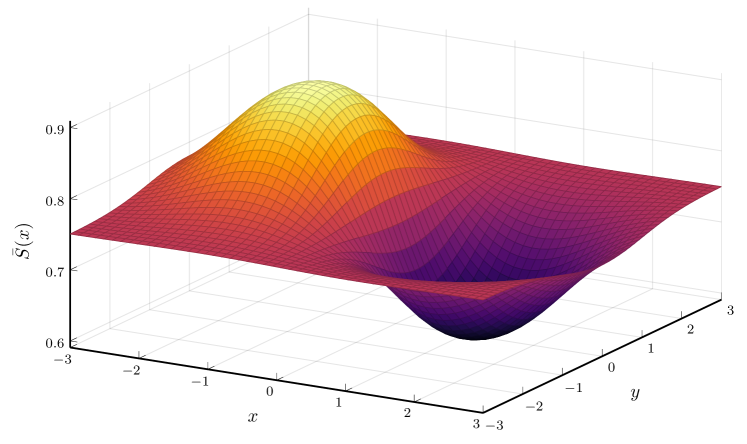
Figure 2: Mean values of the parameters $S$ according to the position of the plant

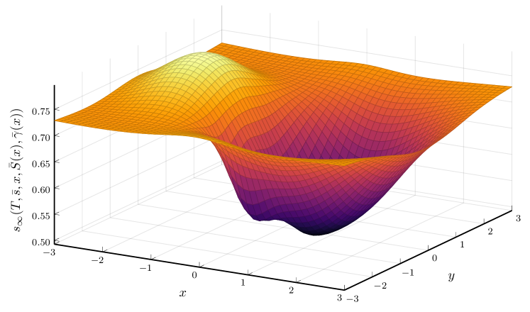
Figure 3: Comparison with the values of the mean-field flow at the final time $\hat{s}_{\infty}(T,\bar{s},x,\bar{S}(x),\bar{\gamma}(x))$ where $\bar{s}=\displaystyle\frac{s_{0}^{\min}+s_{0}^{\max}}{2}$.

4 Conclusion

The model of competition between plants studied in this article is frequently used for its flexibility (by tuning the parameters $\sigma_{x}$ and $\sigma_{r}$) and for its capacity to reproduce the population dynamics observed experimentally. This model has also interesting mathematical properties. Under little restrictive assumptions on the initial conditions and parameters, the dynamics is theoretically guaranteed to remain in a biologically interpretable domain of the phase space. It is also possible to study the behavior of the population when $N\rightarrow\infty$, by simulating the mean-field dynamics, as long as the initial distribution converges to a deterministic probability measure. Finally, the simulations, both at the microscopic and macroscopic scales, seem to indicate that the population tends to a stationary state when $t\rightarrow+\infty$. A future research direction could be to couple this heterogeneous competition model with one of the birth and death processes, and to study the evolution of the heterogeneity of the population.

5 References

1. Adams, T., Ackland, G., Marion, G., & Edwards, C. (2011). Effects of local interaction and dispersal on the dynamics of size-structured populations. Ecological modelling, 222(8), 1414-1422.

2. Adams, T. P., Holland, E. P., Law, R., Plank, M. J., & Raghib, M. (2013). On the growth of locally interacting plants: differential equations for the dynamics of spatial moments. Ecology, 94(12), 2732-2743.

3. Berger, U., Piou, C., Schiffers, K., & Grimm, V. (2008). Competition among plants: concepts, individual-based modelling approaches, and a proposal for a future research strategy. Perspectives in Plant Ecology, Evolution and Systematics, 9(3-4), 121-135.

4. Bolker, B., & Pacala, S. W. (1997). Using moment equations to understand stochastically driven spatial pattern formation in ecological systems. Theoretical population biology, 52(3), 179-197.

5. Bolley, F., Canizo, J. A., & Carrillo, J. A. (2011). Stochastic mean-field limit: non-Lipschitz forces and swarming. Mathematical Models and Methods in Applied Sciences, 21(11), 2179-2210.

6. Beyer, R., Etard, O., Cournède, P. H., & Laurent-Gengoux, P. (2015). Modeling spatial competition for light in plant populations with the porous medium equation. Journal of mathematical biology, 70(3), 533-547.

7. Campillo, F., & Joannides, M. (2009). A spatially explicit Markovian individual-based model for terrestrial plant dynamics. arXiv preprint arXiv:0904.3632.

8. Carrillo, J. A., Goudon, T., Lafitte, P., & Vecil, F. (2008). Numerical schemes of diffusion asymptotics and moment closures for kinetic equations. Journal of Scientific Computing, 36(1), 113-149.

9. Clark, B., & Bullock, S. (2007). Shedding light on plant competition: modelling the influence of plant morphology on light capture (and vice versa). Journal of theoretical biology, 244(2), 208-217.

10. Cournède, P. H., Mathieu, A., Houllier, F., Barthélémy, D., & De Reffye, P. (2008). Computing competition for light in the GREENLAB model of plant growth: a contribution to the study of the effects of density on resource acquisition and architectural development. Annals of Botany, 101(8), 1207-1219.

11. Dobrushin, R. L. V. (1979). Vlasov equations. Functional Analysis and Its Applications, 13(2), 115-123.

12. Fournier, N., & Méléard, S. (2004). A microscopic probabilistic description of a locally regulated population and macroscopic approximations. The Annals of Applied Probability, 14(4), 1880-1919.

13. Golse, F. (2016). On the dynamics of large particle systems in the mean-field limit. In Macroscopic and large scale phenomena: coarse graining, mean field limits and ergodicity (pp. 1-144). Springer, Cham.

14. Lafitte, P., Lejon, A., & Samaey, G. (2016). A high-order asymptotic-preserving scheme for kinetic equations using projective integration. SIAM Journal on Numerical Analysis, 54(1), 1-33.

15. Lagoutière, F., & Vauchelet, N. (2017). Analysis and simulation of nonlinear and nonlocal transport equations. In Innovative Algorithms and Analysis (pp. 265-288). Springer, Cham.

16. Law, R., & Dieckmann, U. (1999). Moment approximations of individual-based models.

17. Lv, Q., Schneider, M. K., & Pitchford, J. W. (2008). Individualism in plant populations: using stochastic differential equations to model individual neighbourhood-dependent plant growth. Theoretical population biology, 74(1), 74-83.

18. Nakagawa, Y., Yokozawa, M., & Hara, T. (2015). Competition among plants can lead to an increase in aggregation of smaller plants around larger ones. Ecological Modelling, 301, 41-53.

19. Paine, C. T., Marthews, T. R., Vogt, D. R., Purves, D., Rees, M., Hector, A., & Turnbull, L. A. (2012). How to fit nonlinear plant growth models and calculate growth rates: an update for ecologists. Methods in Ecology and Evolution, 3(2), 245-256.

20. Rackauckas, C., & Nie, Q. (2017). Differentialequations. jl–a performant and feature-rich ecosystem for solving differential equations in julia. Journal of open research software, 5(1).

21. Schneider, M. K., Law, R., & Illian, J. B. (2006). Quantification of neighbourhood-dependent plant growth by Bayesian hierarchical modelling. Journal of Ecology, 310-321.

22. Tsitouras, C. (2011). Runge–Kutta pairs of order 5 (4) satisfying only the first column simplifying assumption. Computers & Mathematics with Applications, 62(2), 770-775.

23. Varadarajan, V. S. (1958). On the convergence of sample probability distributions. Sankhyā: The Indian Journal of Statistics (1933-1960), 19(1/2), 23-26.

24. Villani, C. (2009). Optimal transport: old and new (Vol. 338, p. 23). Berlin: springer.

25. Weigelt, A., & Jolliffe, P. (2003). Indices of plant competition. Journal of ecology, 707-720.

Appendix A Appendix

A.1 Proof of inequality (49)

Let us express the empirical flow and the mean-field flow (for the simplicity of notation, we omit the reference to $z^{0}_{1:N}$, $\hat{s}_{N}(t,s_{1},\theta_{1},z^{0}_{1:N})=\hat{s}_{N}(t,s_{1},\theta_{1})$)

$$\hat{s}_{N}(t,s_{1},\theta_{1})=s_{m}(s_{1}/s_{m})^{e^{-\gamma_{N}(\theta_{1})t}}\exp\left(\gamma_{N}(\theta_{1})\log(S_{1}/s_{m})\right.$$ (71)

$$\left.\times\int_{0}^{t}\left(1-\frac{N}{N-1}\int_{\mathbb{R}_{+}^{*}\times\mathbb{R}^{2}}C(\hat{s}_{N}(\tau,s_{1},\theta_{1}),s_{1}^{\prime},|x_{1}-x_{1}^{\prime}|)\hat{\mu}_{N}^{s,x}(\tau,ds_{1}^{\prime},x_{1}^{\prime})\right)e^{\gamma_{N}(\theta_{1})(\tau-t)}d\tau\right)$$

$$\text{where }\gamma_{N}(\theta)=\gamma_{N}(x,S,\gamma)=\gamma\left(1-\frac{\log(S/s_{m})}{2(N-1)R_{M}}\right)$$

$$s_{\infty}(t,s_{2},\theta_{2})=s_{m}(s_{2}/s_{m})^{e^{-\gamma_{2}t}}\exp\left(\gamma_{2}\log(S_{2}/s_{m})\phantom{\int_{0}^{t}}\right.$$

$$\times\left.\int_{0}^{t}\left(1-\int_{\mathbb{R}_{+}^{*}\times\mathbb{R}^{2}}C(s_{\infty}(\tau,s_{2},\theta_{2}),s_{2}^{\prime},|x_{2}-x_{2}^{\prime}|)\mu^{s,x}(t,ds^{\prime}_{2},dx^{\prime}_{2})\right)e^{\gamma_{2}(\tau-t)}d\tau\right)$$

Let us consider the function

$$\mathcal{S}:(t,s,\gamma,S,C)\in\mathbb{R}_{+}\times[s_{0}^{\min};s_{0}^{\max}]\times[0;\gamma_{M}]\times[S_{m};s_{m}\exp(R_{M})]\times[-1;1]$$ (72)

$$\mapsto s_{m}\left(\frac{s}{s_{m}}\right)^{e^{-\gamma t}}\left(\frac{S}{s_{m}}\right)^{C}$$

We introduce additional notations for the competition terms. Let $s_{1},s_{2}\in[s_{0}^{\min};s_{0}^{\max}]$ and $\theta_{1}=(x_{1},S_{1},\gamma_{1}),\theta_{2}=(x_{2},S_{2},\gamma_{2})\in\Theta$.

$$C_{N}(t,s_{1},\theta_{1})$$ (73)

$$=\gamma_{N}(\theta_{1})\int_{0}^{t}\left(1-\frac{N}{N-1}\int_{\mathbb{R}_{+}^{*}\times\mathbb{R}^{2}}C(\hat{s}_{N}(\tau,s_{1},\theta_{1}),s_{1}^{\prime},|x_{1}-x_{1}^{\prime}|)\hat{\mu}_{N}^{s,x}(\tau,ds_{1}^{\prime},x_{1}^{\prime})\right)e^{\gamma_{N}(\theta_{1})(\tau-t)}d\tau$$

$$C_{\infty}(t,s_{2},\theta_{2})=\gamma_{2}\int_{0}^{t}\left(1-\int_{\mathbb{R}_{+}^{*}\times\mathbb{R}^{2}}C(s_{\infty}(\tau,s_{2},\theta_{2}),s_{2}^{\prime},|x_{2}-x_{2}^{\prime}|)\mu^{s,x}(t,ds^{\prime}_{2},dx^{\prime}_{2})\right)e^{\gamma_{2}(\tau-t)}d\tau$$

We decompose the difference between the two flows into three terms.

$$\hat{s}_{N}(t,s_{1},\theta_{1})-s_{\infty}(t,s_{2},\theta_{2})=\mathcal{S}(t,s_{1},\gamma_{N}(\theta_{1}),S_{1},C_{N}(t,s_{1},\theta_{1}))-\mathcal{S}(t,s_{1},\gamma_{1},S_{1},C_{N}(t,s_{1},\theta_{1}))$$ (74)

$$+\mathcal{S}(t,s_{1},\gamma_{1},S_{1},C_{N}(t,s_{1},\theta_{1}))-\mathcal{S}(t,s_{2},\gamma_{2},S_{2},C_{N}(t,s_{1},\theta_{1}))$$

$$+\mathcal{S}(t,s_{2},\gamma_{2},S_{2},C_{N}(t,s_{1},\theta_{1}))-\mathcal{S}(t,s_{2},\gamma_{2},S_{2},C_{\infty}(t,s_{2},\theta_{2}))$$

Let us consider the first term.

$$\mathcal{S}_{1}=|\mathcal{S}(t,s_{1},\gamma_{N}(\theta_{1}),S_{1},C_{N}(t,s_{1},\theta_{1}))-\mathcal{S}(t,s_{1},\gamma_{1},S_{1},C_{N}(t,s_{1},\theta_{1}))|$$ (75)

$$\leq\int_{0}^{1}\left|\frac{\partial\mathcal{S}}{\partial\gamma}(t,s_{1},\gamma_{1}+\alpha(\gamma_{N}(\theta_{1})-\gamma_{1}),S_{1},C_{N}(t,s_{1},\theta_{1}))d\alpha\right|.|\gamma_{N}(\theta_{1})-\gamma_{1}|$$

$$\frac{\partial\mathcal{S}}{\partial\gamma}(t,s,\gamma,S,C)=-te^{-\gamma t}s_{m}\log(s/s_{m})\left(\frac{s}{s_{m}}\right)^{e^{-\gamma t}}\left(\frac{S}{s_{m}}\right)^{C}$$

$$\mathcal{S}_{1}\leq\gamma_{1}ts_{1}\log(s_{1}/s_{m})(S_{1}/S_{m})\frac{\log(S_{1}/s_{m})}{2(N-1)R_{M}}$$

Let us consider the second term.

$$\mathcal{S}_{2}=|\mathcal{S}(t,s_{1},\gamma_{1},S_{1},C_{N}(t,s_{1},\theta_{1}))-\mathcal{S}(t,s_{2},\gamma_{2},S_{2},C_{N}(t,s_{1},\theta_{1}))|$$ (76)

$$\frac{\partial\mathcal{S}}{\partial s}(t,s,\gamma,S,C)=e^{-\gamma t}(S/s_{m})^{C}(s/s_{m})^{e^{-\gamma t}-1}$$

$$\left|\frac{\partial\mathcal{S}}{\partial s}(t,s,\gamma,S,C)\right|\leq e^{R_{M}}$$

$$\frac{\partial\mathcal{S}}{\partial S}(t,s,\gamma,S,C)=C\left(\frac{s}{s_{m}}\right)^{e^{-\gamma t}}\left(\frac{S}{s_{m}}\right)^{C-1}$$

$$\left|\frac{\partial\mathcal{S}}{\partial S}(t,s,\gamma,S,C)\right|\leq\frac{s_{0}^{\max}}{s_{m}}$$

$$\mathcal{S}_{2}\leq e^{R_{M}}|s_{1}-s_{2}|+ts^{0}_{\max}\log(s_{0}^{\max}/s_{m})e^{R_{M}}|\gamma_{1}-\gamma_{2}|+(s_{0}^{\max}/s_{m})|S_{1}-S_{2}|$$

Let us consider the third term.

$$\frac{\partial\mathcal{S}}{\partial C}(t,s,\gamma,S,C)=s_{m}\left(\frac{S}{s_{m}}\right)^{C}\log\left(\frac{S}{s_{m}}\right)\left(\frac{s}{s_{m}}\right)^{e^{-\gamma t}}$$ (77)

$$\left|\frac{\partial\mathcal{S}}{\partial C}(t,s,\gamma,S,C)\right|\leq s_{0}^{\max}R_{M}e^{R_{M}}$$

$$|\mathcal{S}(t,s_{2},\gamma_{2},S_{2},C_{N}(t,s_{1},\theta_{1}))-\mathcal{S}(t,s_{2},\gamma_{2},S_{2},C_{\infty}(t,s_{2},\theta_{2}))|\leq$$

$$s_{0}^{\max}e^{R_{M}}R_{M}|C_{N}(t,s_{1},\theta_{1})-C_{\infty}(t,s_{2},\theta_{2})|$$

Let us expand the difference of the competition terms:

$$c_{N}(t,s_{1},\theta_{1})=\int_{\mathbb{R}_{+}^{*}\times\mathbb{R}^{2}}C(\hat{s}_{N}(t,s_{1},\theta_{1}),s^{\prime}_{1},|x_{1}-x^{\prime}_{1}|)\hat{\mu}_{N}^{s,x}(t,ds^{\prime}_{1},dx^{\prime}_{1})$$ (78)

$$c_{\infty}(t,s_{2},\theta_{2})=\int_{\mathbb{R}_{+}^{*}\times\mathbb{R}^{2}}C(s_{\infty}(t,s_{2},\theta_{2}),s^{\prime}_{1},|x_{2}-x^{\prime}_{2}|)\mu(t,ds^{\prime}_{2},dx^{\prime}_{2})$$

$$|C_{N}(t,s_{1},\theta_{1})-C_{\infty}(t,s_{2},\theta_{2})|$$ (79)

$$\leq\left|\int_{0}^{t}\left(1-\frac{N}{N-1}c_{N}(\tau,s_{1},\theta_{1})\right)\left(\gamma_{N}(\theta_{1})e^{\gamma_{N}(\theta_{1})(\tau-t)}-\gamma_{1}e^{\gamma_{1}(\tau-t)}\right)d\tau\right|$$

$$+\left|\int_{0}^{t}\left(1-\frac{N}{N-1}c_{N}(\tau,s_{1},\theta_{1})\right)\left(\gamma_{1}e^{\gamma_{1}(\tau-t)}-\gamma_{2}e^{\gamma_{2}(\tau-t)}\right)d\tau\right|$$

$$+\frac{\gamma_{2}}{N-1}\left|\int_{0}^{t}c_{N}(\tau,s_{1},\theta_{1})e^{\gamma_{2}(\tau-t)}d\tau\right|+\gamma_{2}\int_{0}^{t}\left|c_{N}(\tau,s_{1},\theta_{1})-c_{\infty}(\tau,s_{2},\theta_{2})\right|e^{\gamma_{2}(\tau-t)}d\tau$$

Let us consider the first term.

$$|1-\frac{N}{N-1}c_{N}(\tau,s_{1},\theta_{1})|\leq 1$$ (80)

$$\frac{\partial}{\partial\gamma}\left(\gamma\int_{0}^{t}\left(1-\frac{N}{N-1}c_{N}(\tau,s_{1},\theta_{1})\right)e^{\gamma(\tau-t)}d\tau\right)$$

$$=\int_{0}^{t}\left(1-\frac{N}{N-1}c_{N}(\tau,s_{1},\theta_{1})\right)(1+\gamma(\tau-t))e^{\gamma(\tau-t)}d\tau$$

$$\left|\frac{\partial}{\partial\gamma}\left(\gamma\int_{0}^{t}\left(1-\frac{N}{N-1}c_{N}(\tau,s_{1},\theta_{1})\right)e^{\gamma(\tau-t)}d\tau\right)\right|\leq\int_{0}^{t}(1+\gamma(t-\tau))e^{\gamma(\tau-t)}d\tau$$

$$=\frac{2-e^{-\gamma t}(2+\gamma t)}{\gamma}\leq t$$

We can deduce from the above inequality the following upper-bound on the competition terms.

$$|C_{N}(t,s_{1},\theta_{1})-C_{\infty}(t,s_{2},\theta_{2})|\leq\gamma_{1}t\frac{\log(S_{1}/s_{m})}{2R_{M}(N-1)}+t|\gamma_{1}-\gamma_{2}|+\frac{1}{N-1}$$ (81)

$$+\gamma_{2}\int_{0}^{t}\left|\int_{\mathbb{R}^{*}_{+}\times\Theta}C(\hat{s}_{N}(\tau,s_{1},\theta_{1}),s^{\prime}_{1},|x_{1}-x^{\prime}_{1}|)\hat{\mu}_{N}^{s,x}(\tau,ds^{\prime}_{1},dx^{\prime}_{1})\right.$$

$$\left.-\int_{\mathbb{R}_{+}^{*}\times\Theta}C(s_{\infty}(\tau,s_{2},\theta_{2}),s^{\prime}_{2},|x_{2}-x^{\prime}_{2}|)\mu(\tau,ds^{\prime}_{2},dx^{\prime}_{2})\right|e^{\gamma_{2}(\tau-t)}d\tau$$

We use the coupling $\pi_{0}$ introduced at the beginning of the proof to express the last term.

$$\left|\int_{\mathbb{R}^{*}_{+}\times\Theta}C(\hat{s}_{N}(t,s_{1},\theta_{1}),s^{\prime}_{1},|x_{1}-x^{\prime}_{1}|)\hat{\mu}_{N}^{s,x}(t,ds^{\prime}_{1},dx^{\prime}_{1})\right.$$ (82)

$$\left.-\int_{\mathbb{R}_{+}^{*}\times\Theta}C(s_{\infty}(t,s_{2},\theta_{2}),s^{\prime}_{2},|x_{2}-x^{\prime}_{2}|)\mu(t,ds^{\prime}_{2},dx^{\prime}_{2})\right|$$

$$\leq \iint_{(\mathbb{R}_{+}^{*}\times\Theta)^{2}}|C(\hat{s}_{N}(t,s_{1},\theta_{1}),\hat{s}_{N}(t,s^{\prime}_{1},\theta^{\prime}_{1}),|x_{1}-x^{\prime}_{1}|)-C(s_{\infty}(t,s_{2},\theta_{2}),s_{\infty}(t,s_{2},\theta^{\prime}_{2}),|x_{2}-x^{\prime}_{2}|)|$$ (83)

$$\times\pi_{0}(ds^{\prime}_{1},d\theta_{1}^{\prime},ds^{\prime}_{2},d\theta^{\prime}_{2})$$

We compute the derivatives of the competition potential to obtain upper-bounds of the variations. For any $\tilde{s}_{1}\in[s_{m}^{N};\hat{S}_{N}(S_{1})]$, any $\tilde{s}_{2}\in[s_{m};S_{2}]$, and $\delta\geq 0$, we have

$$\frac{\partial C}{\partial s}(\tilde{s}_{1},\tilde{s}_{2},\delta)=-\frac{\log(\tilde{s}_{2}/s_{m})(1-\tanh^{2}(\frac{1}{\sigma_{r}}\log(\tilde{s}_{2}/\tilde{s}_{1})))}{2R_{M}\tilde{s}_{1}\sigma_{r}(1+\delta^{2}/\sigma_{x}^{2})}$$ (84)

$$\left|\frac{\partial C}{\partial s}(\tilde{s}_{1},\tilde{s}_{2},\delta)\right|\leq\frac{1}{2s^{N}_{m}\sigma_{r}}$$

$$\frac{\partial C}{\partial s^{\prime}}(\tilde{s}_{1},\tilde{s}_{2},\delta)=\frac{\sigma_{x}^{2}(\sigma_{r}(1+\tanh(\frac{1}{\sigma_{r}}\log(\tilde{s}_{2}/\tilde{s}_{1}))+\log(\tilde{s}_{2}/\tilde{s}_{1})(1-\tanh^{2}(\frac{1}{\sigma_{r}}\log(\tilde{s}_{2}/\tilde{s}_{1}))))}{2R_{M}\tilde{s}_{2}\sigma_{r}(\sigma_{x}^{2}+\delta^{2})}$$

$$\left|\frac{\partial C}{\partial s^{\prime}}(\tilde{s}_{1},\tilde{s}_{2},\delta)\right|\leq\frac{2\sigma_{r}+R_{M}}{2R_{M}s_{m}\sigma_{r}}$$

$$\frac{\partial C}{\partial\delta^{2}}(\tilde{s}_{1},\tilde{s}_{2},\delta)=-\frac{\log(\tilde{s}_{2}/s_{m})(1+\tanh(\frac{1}{\sigma_{r}}\log(\tilde{s}_{2}/\tilde{s}_{1})))}{2R_{M}\sigma_{x}^{2}(1+\delta^{2}/\sigma_{x}^{2})^{2}}$$

$$\left|\frac{\partial C}{\partial\delta^{2}}(\tilde{s}_{1},\tilde{s}_{2},\delta)\right|\leq\frac{1}{\sigma_{x}^{2}}$$

It follows that

$$\iint_{(\mathbb{R}_{+}^{*}\times\Theta)^{2}}|C(\hat{s}_{N}(t,s_{1},\theta_{1}),\hat{s}_{N}(t,s^{\prime}_{1},\theta^{\prime}_{1}),|x_{1}-x^{\prime}_{1}|)$$ (85)

$$-C(s_{\infty}(t,s_{2},\theta_{2}),s_{\infty}(t,s_{2},\theta^{\prime}_{2}),|x_{2}-x^{\prime}_{2}|)|\pi_{0}(ds^{\prime}_{1},d\theta_{1}^{\prime},ds^{\prime}_{2},d\theta^{\prime}_{2})$$

$$\leq\frac{|\hat{s}_{N}(t,s_{1},\theta_{1})-s_{\infty}(t,s_{2},\theta_{2})|}{2s_{m}^{N}\sigma_{r}}$$

$$+\frac{2\sigma_{r}+R_{M}}{2R_{M}s_{m}\sigma_{r}}\iint_{(\mathbb{R}_{+}^{*}\times\Theta)^{2}}|\hat{s}_{N}(t,s^{\prime}_{1},\theta_{1}^{\prime})-s_{\infty}(t,s^{\prime}_{2},\theta^{\prime}_{2})|\pi_{0}(ds^{\prime}_{1},d\theta^{\prime}_{1},ds^{\prime}_{2},d\theta^{\prime}_{2})$$

$$+\frac{|x_{1}-x_{2}|}{\sigma_{x}^{2}}\int_{\mathbb{R}^{2}}|x_{1}+x_{2}-2x^{\prime}_{2}|\mu_{0}^{x}(dx^{\prime}_{2})$$

$$+\frac{1}{\sigma_{x}^{2}}\iint_{\mathbb{R}^{4}}|x^{\prime}_{1}+x^{\prime}_{2}-2x_{1}|.|x^{\prime}_{1}-x^{\prime}_{2}|\pi_{0}^{x}(dx^{\prime}_{1},dx^{\prime}_{2})$$

For the last terms relative to $x$, we have used the relation

$$|x_{1}-x_{1}^{\prime}|^{2}-|x_{2}-x^{\prime}_{2}|^{2}=(x_{1}+x_{2}-2x^{\prime}_{2}).(x_{1}-x_{2})+(x^{\prime}_{1}+x^{\prime}_{2}-2x_{1}).(x^{\prime}_{1}-x^{\prime}_{2})$$ (86)

Let us further consider the $x$ terms.

$$\int_{\mathbb{R}^{2}}|x_{1}+x_{2}-2x^{\prime}_{2}|\mu_{0}^{x}(dx^{\prime}_{2})\leq|x_{1}+x_{2}|+2\int_{\mathbb{R}^{2}}|x^{\prime}_{2}|\mu_{0}^{x}(dx^{\prime}_{2})$$ (87)

$$\iint_{\mathbb{R}^{4}}|x^{\prime}_{1}+x^{\prime}_{2}-2x_{1}|.|x^{\prime}_{1}-x^{\prime}_{2}|\pi_{0}^{x}(dx^{\prime}_{1},dx^{\prime}_{2})$$

$$\leq\sqrt{\iint_{\mathbb{R}^{4}}|x^{\prime}_{1}+x^{\prime}_{2}-2x_{1}|^{2}\pi^{x}_{0}(dx^{\prime}_{1},dx^{\prime}_{2})}.\sqrt{\iint_{\mathbb{R}^{4}}|x^{\prime}_{1}-x^{\prime}_{2}|^{2}\pi^{x}_{0}(dx^{\prime}_{1},dx^{\prime}_{2})}$$

$$\iint_{\mathbb{R}^{4}}|x^{\prime}_{1}+x^{\prime}_{2}-2x_{1}|^{2}\pi_{0}^{x}(dx^{\prime}_{1},dx^{\prime}_{2})$$

$$\leq 2\int_{\mathbb{R}^{2}}|x^{\prime}_{1}|^{2}\hat{\mu}_{N}^{x}(0,dx^{\prime}_{1})+2\int_{\mathbb{R}^{2}}|x^{\prime}_{2}|^{2}\mu_{0}^{x}(dx^{\prime}_{2})-4x_{1}.\left(\int_{\mathbb{R}^{2}}x^{\prime}_{1}\hat{\mu}_{N}^{x}(0,dx^{\prime}_{1})+\int_{\mathbb{R}^{2}}x^{\prime}_{2}\mu_{0}^{x}(dx^{\prime}_{2})\right)$$

$$=k^{x}(x_{1},\hat{\mu}_{N}^{x}(0),\mu_{0}^{x})^{2}$$

We gather all the previous inequalities to obtain an upper-bound on the gap between the microscopic and the mean-field flows:

$$|\hat{s}_{N}(t,s_{1},\theta_{1})-s_{\infty}(t,s_{2},\theta_{2})|\leq\frac{\gamma_{1}ts_{1}\log(s_{1}/s_{m})(S_{1}/s_{m})\log(S_{1}/s_{m})}{2R_{M}(N-1)}+e^{R_{M}}|s_{1}-s_{2}|$$ (88)

$$+ts^{0}_{\max}\log(s_{0}^{\max}/s_{m})e^{R_{M}}|\gamma_{1}-\gamma_{2}|+(s_{0}^{\max}/S_{m})|S_{1}-S_{2}|$$

$$+s_{0}^{\max}e^{R_{M}}R_{M}\left(\gamma_{1}t\frac{\log(S_{1}/s_{m})}{2R_{M}(N-1)}+t|\gamma_{1}-\gamma_{2}|+\frac{1}{N-1}\right)$$

$$+s_{0}^{\max}e^{R_{M}}R_{M}\gamma_{M}\int_{0}^{t}\left(\frac{|\hat{s}_{N}(\tau,s_{1},\theta_{1})-s_{\infty}(\tau,s_{2},\theta_{2})|}{s_{m}^{N}\sigma_{r}}\right.$$

$$+\frac{2\sigma_{r}+R_{M}}{2R_{M}s_{m}\sigma_{r}}\iint_{(\mathbb{R}_{+}^{*}\times\Theta)^{2}}|\hat{s}_{N}(\tau,s^{\prime}_{1},\theta^{\prime}_{1})-s_{\infty}(\tau,s_{2}^{\prime},\theta^{\prime}_{2})|\pi_{0}(ds^{\prime}_{1},d\theta^{\prime}_{1},ds^{\prime}_{2},d\theta^{\prime}_{2})$$

$$+\frac{1}{\sigma_{x}^{2}}\left(|x_{1}+x_{2}|+\int_{\mathbb{R}^{2}}|x|\mu_{0}^{x}(dx)\right)|x_{1}-x_{2}|$$

$$\left.+\frac{k^{x}(x_{1},\hat{\mu}_{N}^{x}(0),\mu_{0}^{x})}{\sigma_{x}^{2}}\iint_{\mathbb{R}^{4}}|x_{1}^{\prime}-x^{\prime}_{2}|\pi_{0}^{x}(dx^{\prime}_{1},dx^{\prime}_{2})\right)d\tau$$

Finally, we obtain the required inequality by integrating over $\pi_{0}$.

A.2 Parameters values chosen for the simulations in section 2.4.2

initial size	$s_{0}=0.1$
Extremal sizes	$s_{m}=5\times 10^{-2}$, $R_{M}=3$
Position variance	$L=1$
Extremal values of $\bar{S}(x)$	$S_{m}=0.5$, $S_{M}=1.0$, $S_{0}=0.75$
Positions of $\bar{S}(x)$ extrema	$x_{\max}^{S}=(-L,0)$, $x_{\min}^{S}=(L,0)$
Spatial curvatures of $\bar{S}(x)$	$H_{\max}^{S}=H_{\min}^{S}=\mathrm{I}_{2}/L^{2}$
Standard deviation of $S$	$\delta S=0.1$
Extremal values of $\bar{\gamma}(x)$	$\gamma_{M}=2$,$\gamma_{m}=0.1$,$\gamma_{0}=1.05$
Positions of $\bar{\gamma}(x)$ extrema	$x_{\min}^{\gamma}=(0,-L),~{}x_{\max}^{\gamma}=(0,L)$
Spatial curvature of $\bar{\gamma}(x)$	$H_{\max}^{\gamma}=H_{\min}^{\gamma}=\mathrm{I}_{2}/L^{2}$
Standard deviation of $\gamma$	$\delta\gamma=0.1$
Competition parameters	$\sigma_{r}=1.32$, $\sigma_{x}=L/2$

A.3 Parameters values chosen for the simulations in section 3.4

Bounds of the initial size	$s_{0}^{\min}=0.1,~{}s_{0}^{\max}=0.3$
Time step and time horizon	$\Delta t=1$, $T=10$
sample size	$N=1~{}000$
size of training and testing sets	$K=1~{}000$
initial degree of polynomial	$\deg(f^{3}_{d})=5$
other degree	$\deg(f^{5}_{d})=3$

A.4 R² quantifying the reconstruction of the competition potential of the simulation in section 3.4

Time	$R^{2}$ associated with the potential reconstruction
0	0.993
1	0.976
2	0.978
3	0.980
4	0.980
5	0.980
6	0.980
7	0.981
8	0.981
9	0.981