Sea: A lightweight data-placement library for Big Data scientific computing

Abstract

The recent influx of open scientific data has contributed to the transitioning of scientific computing from compute intensive to data intensive. Whereas many Big Data frameworks exist that minimize the cost of data transfers, few scientific applications integrate these frameworks or adopt data-placement strategies to mitigate the costs. Scientific applications commonly rely on well-established command-line tools that would require complete reinstrumentation in order to incorporate existing frameworks. We developed Sea as a means to enable data-placement strategies for scientific applications executing on HPC clusters without the need to reinstrument workflows. Sea leverages GNU C library interception to intercept POSIX-compliant file system calls made by the applications. We designed a performance model and evaluated the performance of Sea on a synthetic data-intensive application processing a representative neuroimaging dataset (the Big Brain). Our results demonstrate that Sea significantly improves performance, up to a factor of 3$\times$.

1 Introduction

Efficient data-placement strategies have become essential to minimizing Big Data processing overheads. These strategies, such as data locality and in-memory computing, improve application runtime by ensuring data accesses occur on the most efficient available storage. Existing Big Data frameworks, such as MapReduce [5], Apache Spark [21] and Dask [13], improve runtime performance through the incorporation of data-placement strategies.

Until the recent surge in publicly available scientific data, scientific workflows have been regarded as compute intensive. As a result, standardized scientific tools typically lack data-placement mechanisms. In contrast, efforts have been placed on efficient storage representation, such as HDF5 [8] and Zarr [11], and the sharing of data, through initiatives like DataLad [19].

Data-placement strategies can complement existing solutions by facilitating the transfer and processing of large datasets across different infrastructures, and placing the different file formats at the preferred storage layer to maximize efficiency. However, adapting existing scientific applications to Big Data frameworks requires considerable effort, necessitating the rewrite of many well-established applications. Furthermore, as noted in [10], Big Data frameworks are not easy to use for the processing of certain scientific data, such as imaging data, due to the level of expertise required to rewrite reference implementations using the frameworks.

Our goal is to provide a data-placement solution to standardized scientific computing applications executing on High Performance Computing (HPC) clusters. The applications of interest to us consist of various tasks that communicate to each other via a POSIX-compliant file system. Whereas the application can be platform-agnostic, we assume users will leverage them within an linux-based HPC context, particularly when processing large volumes of data, due to their inherent reliance on POSIX-compliance.

We developed Sea, a user-space data-placement library that provides efficient data placement without reinstrumentation of the underlying application. Given a predefined storage hierarchy, Sea can prefetch, cache, flush, and evict data to and from a permanent storage location.

To provide a frame-of-reference for Sea’s performance on HPC systems, we designed a performance model. We then evaluated Sea’s performance on a synthetic Big Data application running on a representative neuroimaging dataset, comparing its performance with the bounds delineated by the model.

2 Related Work

2.1 HPC Infrastructure

The general structure of HPC clusters complicates the deployment of Big Data frameworks. Typical HPC clusters consist of distinct storage and compute nodes. While compute nodes may also have local storage, there is no distributed file system like the Hadoop Distributed File System (HDFS) [15] or Alluxio [9] to facilitate data locality. Furthermore, access to these compute nodes is ephemeral, with allocation duration enforced by a batch scheduler. Therefore, any data written to compute nodes are rendered inaccessible after the allocation is terminated.

The storage layer found on HPC clusters consists of a high-performance parallel file system (PFS) (e.g., Lustre [14]). These file systems are shared amongst all compute nodes within a cluster, typically connected to the nodes via high-performance network interconnect like InfiniBand [12]. I/O overheads of shared PFS can be incurred in many places, from the shared network to the bandwidth and latency of the storage devices. With Lustre specifically, there typically are many data nodes, known as Object Storage Servers (OSS) which contain several storage devices, known as Object Storage Targets (OST). All file metadata is maintained within a separate node known as the Metadata Server (MDS) and stored within a device referred to as the Metadata Target (MDT). Although data transfers can be communicated directly to the corresponding OST, the clients need to first communicate with the MDS to determine which OST to communicate with. This can result in major data transfer overheads, particularly when making numerous requests to the metadata server.

HPC clusters may provide a faster intermediate storage layer, known as a Burst Buffer, aimed at improving I/O performance. A Burst Buffer typically consists of higher-performance storage devices (SSD and memory) and can be local to the compute node or as a dedicated I/O node. Burst Buffers were introduced as a response to offset the impacts of large-scale application checkpointing on the PFS [4]. The application would write a checkpoint to the Burst Buffer and resume processing, while the checkpoint would be asynchronously flushed to the PFS.

2.2 Big Data Frameworks and File systems

Early Big Data frameworks, notably MapReduce [5] and Apache Spark [21] have implemented and popularized data-management strategies to minimize data transfers at processing time. These strategies are known as data locality and in-memory computing. Data locality ensures that compute tasks are scheduled nearest to where the data is located. Historically, storage and compute nodes were distinct layers, transferring data to the compute location whenever necessary. Rather than transferring large amounts of data over the network to compute tasks, which could incur significant overheads, Big Data frameworks ensure that data is stored directly on the compute nodes. When a compute task requires access to specific data, the scheduler sends the task to the nearest available node to the data, thereby minimizing any cost of network-related data transfers. This strategy is not only used by Big Data Frameworks such as Hadoop MapReduce, Apache Spark, and Dask [13], but also enabled by file systems such as HDFS and Alluxio.

In-memory computing complements data locality by maximizing use of available memory to maintain intermediate data. Whereas with data locality alone, tasks would leverage local storage, typically in the form of HDDs or SSD, to maintain task input and output data, with the addition of in-memory computing, data would be stored in main memory to minimize latency and maximize bandwidth.

While Big Data frameworks and filesystems are not commonly used in HPC, HPC clusters are typically Linux-based and benefit from the Linux page cache, which can provide data locality and in-memory computing at a limited capacity. Furthermore, HPC architectures may also provide an intermediate storage layer, known as a Burst Buffer, to improve application I/O-related overheads. To facilitate an application’s interaction between application and storage layer, distributed file systems have been developed.

2.3 The Linux page cache

While scientific applications do not customarily leverage data-placement strategies and may perform large over-the-network data transfers, they may still benefit from in-memory computing and data locality through the Linux Page Cache [16]. Similarly to other file systems, Lustre leverages the compute node page cache to reduce I/O overheads. System memory is composed of two components: 1) anonymous memory and 2) page cache. Anonymous memory consists of all application-related objects, whereas page cache consists of recently accessed file data. When a file is read, that file is loaded up into the page cache to be flagged for eviction based on a least recently used (LRU) policy. That means subsequent accesses to that data may be done entirely in memory so long as the data has not already been evicted. Similarly, for writes to a file system with writeback cache enabled, the file will be written to memory completing the write operation once the file has been written entirely to memory. That file will then be flushed asynchronously to the appropriate storage device. As system memory may get overloaded with too many write requests, there is a limit to the amount of written data that can exist in memory, known as the dirty_ratio. Furthermore, applications producing too many write requests may be throttled by the system.

2.4 File System implementations

Due to the architecture of conventional HPC clusters, network-based parallel files systems are favoured over Big Data distributed file systems. Such file systems require super-user access, preventing users from deploying their own on-the-fly cluster. While HDFS can be loaded in user-space by mounting its FUSE (Filesystem in User Space) implementation, FUSE-based file systems may perform significantly worse than desired, depending on the application [17]. Even with a user-space version of HDFS, there would be no mechanism to transfer all the data back to the PFS post-processing.

However, there exist Big Data file systems, such as XtreemFS [3], that exist entirely within user space, are POSIX-compliant, and can use alternative methods to FUSE to function. For instance, XtreemFS uses the LD_PRELOAD trick to intercept file system calls made to the GNU C library (glibc). There are limitations to using glibc interception; the application must be dynamically-linked and make glibc calls. However, statically-linked applications are uncommon and applications interacting with POSIX-compliant file systems on Linux machines, the predominant OS of HPC clusters, will make glibc calls. Nevertheless, alternatives to glibc intercept exist that can bypass the aforementioned issues, such as system call interception, but they result in greater overheads [2].

Due to complex file system deployment and configuration properties, XtreemFS is unlikely to be deployed on an ephemeral burst buffer. It also does not provide a simple way to leverage different classes of storage devices, nor ensure that required data will be copied to the cluster’s parallel file system.

BurstFS [20] and GekkoFS [18] are two user-space file systems that are specifically designed with HPC Burst Buffers. That is, both of these file systems are designed to support the ephemeral nature of HPC compute nodes and their associated storage. Additionally, these implementations exist entirely in user-space leveraging the LD_PRELOAD trick to intercept necessary library calls. Whereas these libraries incorporate a client-server architecture to aid in transferring data between nodes, Sea opts for a more lightweight approach ensuring decentralization, statelessness and leveraging underlying file systems for communication and consistency.

3 Materials and Methods

3.1 Sea design and implementation

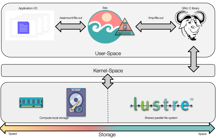
Figure 1: The Sea data-placement library. Sea intercepts I/O-related glibc calls issued by the application and translates the path provided if located within the Sea mountpoint. Sea leverages a user-defined storage hierarchy to help select the most appropriate path and the redirects the call to glibc to process the request on the translated path.

Sea is an open-source user-space data-placement C++ library for applications running on HPC systems. Its main aim is to reduce application data transfer costs by leveraging node-local storage (Figure 1). Sea redirects files accessed from a user-specified mount point to the appropriate storage devices using glibc interception. Within an intercepted call the file will be written to or read from the fastest storage device available.

Sea requires minimal configuration for use. In order to work, Sea requires the user to specify at least two storage devices, a fast temporary device used as cache and a slower long-term storage device. This could be RAM and SSD if working on a single node, or a compute-local SSD and a shared PFS, in the case of an HPC cluster. Ideally, a user will provide a multitude of ephemeral storage devices to improve Sea’s efficacy. Furthermore, to maximize usage of the fastest available storage devices, Sea will allow the user to outline which files can be removed from short-term storage in addition to which files need to be materialized onto long-term storage. Eviction of files is important as this will allow Sea to maximize usage of short-term storage.

Sea was created as a data-placement service to be employed at the discretion of the users on scientific applications. When developing the idea for Sea, we observed the design differences between Big Data and scientific, specifically neuroimaging, frameworks and applications. Scientific frameworks and applications tend to favour ease-of-use, reproducibility, portability and parallelism over minimizing data transfers[7, 6, 19]. It was important for us to ensure that Sea would preserve the design decisions of the underlying tools. Sea achieves this by having few dependencies, is lightweight, and requires minimal configuration.

In this subsection, we will discuss and outline the various design and implementation details made. Furthermore, we will go into detail into the functionality of Sea.

3.1.1 Requirements and assumptions

Sea removes the need to implement the logic to redirect data to the appropriate storage locations. Furthermore, it implements logic to ensure that files are written to the best possible location at any given time. It is both pipeline and infrastructure agnostic.

As it executes in user-space, root permissions are not required, enabling users to use Sea on most Linux-based systems available to them. This differs from Big Data file systems which may require elevated permissions to install. The overhead of intercepting glibc calls is minimal, and negligible compared to system call interception and file systems such as FUSE.

Unlike Big Data frameworks, Sea does not require reinstrumentation of the existing pipelines, allowing users to gain an instant performance boost.

Sea is primarily designed to work with workloads that generate large amounts of intermediate data. Since data must be read from the slower storage device and final outputs will also have to be written to the same device, the use of Sea with workloads that do not produce intermediate data would result in limited speedup and may even introduce some overheads.

Sea provides two main modes based on flushing specification: In-memory computing and copy-all. In-memory computing is achieved when intermediate need not be materialized to long-term storage (i.e. no flushing). With Sea in-memory, we can expect speedups comparable to Big Data frameworks.

As the name implies, Sea copy-all is applicable when all data must be materialized to long-term storage (i.e. flush everything). This can be coupled with eviction to limit the amount of data that will be written to slower, but larger, local storage devices. While this option will have overheads, due to the need to flush all application data, overheads will be negligible when data transfer and compute time are similar.

One important assumption that must be made is that the amount of data produced by the workload far exceeds the amount of page cache space available and utilized by the different file systems. In the case where all workload data can fit into page cache memory, the benefit of Sea may be greatly diminished if not negligible.

Naturally, the amount of data written may not fit entirely into a single local storage location. Currently, the user cannot specify the maximum amount of space to use in a given mountpoint explicitly. Sea queries all the available file systems directly to determine the amount of available space. It relies on user-specified information on the maximum file size produced by the pipeline and the number of concurrent pipeline parallel threads to determine if there is sufficient space to write to the file system without issue. While it prevents overheads due to locking, it makes the assumption that the user is alone writing to the storage device. The user can reduce the amount of local storage space used by increasing the maximum file size of the application.

3.1.2 Glibc interception

Glibc interception is achieved by writing wrappers to existing glibc functions. Most importantly, every glibc function accepting a file path as input parameter needs to be wrapped. The wrappers take any input filepath that is located within the user-provided Sea mountpoint and convert it to a filepath pointing to the best available storage device.

Sea does not currently support the partitioning of files across multiple devices. Since it cannot predict the size of the outputs to ensure the existence of sufficient space on storage devices, the user must provide within the Sea configuration file the maximum file size produced by the workflow. Together with the specified amount of parallel processes, Sea calculates the minimum space required on a storage device to write the file to it. Sea will then go through the hierarchy of available storage devices and select the fastest storage device with sufficient available space. While this process may result in not utilizing all available space in fast storage devices, it will still allow users to gain a performance speedup on the pipeline given that the number of threads multiplied by the file size does not exceed storage space.

3.2 Testing

To work effectively, Sea has to intercept every glibc function that interacts with files or directories. Failure to intercept some of these function may result in the whole application crashing. This is because only Sea can translate the Sea mountpoint file paths to their respective real locations. Due to an absence of standardized glibc testing suites, we developed our own integration tests.

Our tests have been executed on three different operating systems: Ubuntu (xenial, bionic, focal), Fedora (32, 33, 34) and Centos (6, 7). Using this test matrix, the Sea tests were able to span seven glibc versions ranging from 2.17 to 2.33. As glibc file system functions may change over time, Sea behaviour with newer and older versions of glibc is unknown.

3.3 Memory-management

Mode	.sea_flushlist	.sea_evictlist
Copy	yes	no
Remove	no	yes
Move	yes	yes
Keep	no	no

TABLE I: Sea’s memory management modes

Memory-management is an integral component of Sea as de-allocating data from cache makes room for future files to be stored within the higher-performance storage devices. Generalizing an efficient memory-management strategy across all applications is a challenging task. Since Sea works on a per-application basis, memory-management in Sea is application-specific, configured via two files: .sea_flushlist and .sea_evictlist.

Memory management in Sea consists of four different modes, as described in Table I: copy, remove, move and keep. A copy copies a file located within the Sea cache to persistent storage. This operation is particularly useful when a file will be reused by the application, and thus benefits from remaining in cache, but also needs to be communicated between other nodes or needs to be persisted for post-processing analysis. To copy a file, the file must only be specified in the .sea_flushlist.

Remove is for files that are located within a Sea cache, but do not need to be persisted and will not be reused by the pipeline and therefore do not need to occupy cache space. Remove is useful for removing unnecessary application log files. To remove a file, the file must only be specified in the .sea_evictlist.

Similar to the copy, the move mode copies data from cache to persistent storage. However, the assumption here is that these files will not be reused by the application and therefore need not occupy space in cache. Move is therefore synonymous with a copy-and-remove operation and is invoked on files that are specified in both the .sea_flushlist and .sea_evictlist.

Keep is useful for when file needs to be in cache as it will be reused by the application, but is not needed in post-processing analysis or by other nodes.

A third text file, namely the .sea_prefetchlist, exists that can be populated by input files to be prefetched. At this time, Sea cannot determine when prefetched files are no longer needed by the pipeline, and therefore should not be evicted. For files to be prefetched, they must be located within Sea’s mountpoint at startup.

3.4 The Sea and Lustre model

Experimental results can be prone to error and variability, particularly in instances where there a many factors at play, such as in distributed cluster environments. To improve confidence in our experimental results, we developed a simplified performance model that could help describe the behaviours observed in our experimental results. Since different PFS may operate differently, our baseline model will be based on Lustre which is commonly used on HPC infrastructure.

For data-intensive use cases, the makespan models for both Lustre and Sea can be broken down into two components: The amount of time it takes read the data and the amount of time it takes to write the data. With more heterogeneous applications (some components are compute-intensive whereas others are data-intensive), a third component, consisting of compute time, can be added. Furthermore, latency may also play a significant role in an application makespan, particularly in scenarios with large amounts of small files. We choose to ignore latency costs in our model and make the assumption that the application bottleneck is the bandwidth, however, for more accurate estimates we might consider the addition of file system latency, as a fourth model component.

A simplified version of the Lustre makespan model can be defined as follows:

$$M_{l}=\frac{D_{r}}{L_{r}}+\frac{D_{w}}{L_{w}}$$ (1)

Where,
$M_{l}$ is the application makespan using Lustre
$D_{r}$ is the amount of data read
$D_{w}$ is the amount of data written
$L_{r}$ is Lustre’s read bandwidth
$L_{w}$ is Lustre’s write bandwidth

To determine the Lustre bandwidth, one must consider the three components involved: 1) the network bandwidth of the compute nodes, 2) the network bandwidth of the data nodes, and 3) the collective bandwidth of the Lustre storage devices. Depending on each component’s respective values, either of the three may be the source of a bottleneck. The Lustre bandwidth read and write models can therefore be described as follows:

$$L_{r}=\min{(cN,sN,d_{r}\min{(d,cp)})}$$ (2)

and

$$L_{w}=\min{(cN,sN,d_{w}\min{(d,cp)})}$$ (3)

Where,
$N$ is the network bandwidth
$c$ is the number of compute nodes used
$s$ is the number of Lustre storage nodes
$p$ is the number of parallel application processes
$d$ is the number of Lustre storage disks
$d_{r}$ is the read bandwidth of a single Lustre storage disk
$d_{w}$ is the write bandwidth of a single Lustre storage disk

For the sake of simplicity, the above models assume that the network bandwidth between the compute and data nodes is the same. However, this may not necessarily be the case. Furthermore, the model also assumes that each file can only be located on a single disk, meaning that the parallel bandwidth can at maximum be as fast as all Lustre disks combined and as slow as the minimum number of compute threads reading and writing files.

As with many file systems, page cache plays an important role in the speed of application read and writes in Lustre. Since the effects of page cache may be non-negligible given amount of memory available and the data accessed during the execution of the application, it is important to include it in our model. The makespan of an application I/O to and from page cache, $M_{c}$, can be described as in Equation 1, where it is assumed that none of the data is written or read from page cache.

$$M_{c}=\frac{D_{cr}}{cC_{r}}+\frac{D_{cw}}{cC_{w}}$$ (4)

Where,
$M_{c}$ is the makespan of application I/O to page cache
$D_{cr}$ is the amount of data read from cache
$D_{cw}$ is the amount of data written to cache
$C_{r}$ is the page cache read bandwidth
$C_{w}$ is the page cache write bandwidth

As each individual compute node has its own set of memory, we treat the total memory bandwidth as the sum of the individual memory bandwidth of each compute node.

Page cache is difficult to summarize accurately within a model. For one, we must not only consider available memory and anonymous memory used by the application, but we must also consider which pages are candidates for eviction and which files they belong to. In addition, in the case of writes, we must consider asynchronous flushing and the throttling that may occur as a consequence of surpassing the dirty_ratio. Furthermore, Lustre also has its own user-defined settings for how it interacts with the cache that would add additional complexities to the model. As a result, we assume two possible scenarios, one in which page cache is never used (Equation 1) and one in which all application I/O occurs entirely within page cache, excluding the first read which must occur on Lustre (Equation 5). These two models allow us to define the bounds of Lustre’s performance.

$$M_{lc}=\frac{D_{I}}{L_{r}}+M_{c}$$ (5)

Where,
$M_{lc}$ is the application makespan using Lustre with page cache
$D_{I}$ is the amount of input data
$L_{r}$ is the Lustre read bandwidth
$M_{c}$ is the application makespan on page cache

Sea’s model is more complex than Lustre’s as there can be several layers of different devices. For instance, Sea’s model can be defined as:

$$M_{S}=\frac{D_{I}}{L_{r}}+M_{1}+\cdots+M_{n}$$ (6)

Here, $M_{n}$ represents the makespans of the different possible storage levels (e.g., tmpfs, NVMe, SSD, HDD, Lustre) and $M_{S}$ represent the makespan of an application reading and writing to Sea. For our model, we will assume three storage layers: 1) fast tmpfs, 2) intermediate local SSD storage, and 3) slow parallel file system layer. It is important to note that the model assumes that I/O never occurs in distinct storage layers in parallel. Although Sea tries to exhaust the layers, starting from the fastest, it is nevertheless possible that Sea writes to two storage layers at the same time, for instance, when one becomes full and another parallel thread needs to perform a write.

Since the modelling of page cache is even more challenging with Sea due to the additional tmpfs and SSD layer, we will will model the upper and lower performance bounds, as we did with Lustre. Using the three layers and disregarding any possible effects of caching, we can redefine the Sea model to be:

$$M_{S}=M_{SL}+M_{Sg}+M_{St}$$ (7)

Where,
$M_{S}$ is the makespan of an application using Sea
$M_{SL}$ is the makespan of the Sea I/O to Lustre
$M_{Sg}$ is the makespan of the Sea I/O to local disks
$M_{St}$ is the makespan of the Sea I/O to tmpfs

The tmpfs component of the Sea makespan can be defined as the amount of data that can be written ($D_{tw}$) to and read ($D_{tr}$) from tmpfs over its respective bandwidths ($C_{r}$ and $C_{w}$). In other words:

$$M_{St}=\frac{D_{tr}}{cC_{r}}+\frac{D_{tw}}{cC_{w}}$$ (8)

$$D_{tr}=\min\left(D_{m},\max{\left(c(t-pF),0\right)}\right)$$

$$D_{tw}=\min\left(D_{m}+D_{f},\max{\left(c(t-pF),0\right)}\right)$$

Where,
$D_{tr}$ is the amount of data read from tmpfs
$D_{tw}$ is the amount of data written to tmpfs
$D_{m}$ is the amount of intermediate data
$D_{f}$ is the amount of final output data
$t$ is the amount of available space on tmpfs
$F$ is the size of a single file

In an optimal scenario all intermediate data and final output data would fit in tmpfs. This would provide an application using Sea in-memory performance. However, due to limited tmpfs storage space, it is unlikely to be the case. In addition, Sea may further restrict available storage space to prevent exceeding tmpfs storage by ensuring that there is at least sufficient space for all processes to each write a file concurrently.

The local disk makespan model is similar to the tmpfs makespan model, although we must disregard any data that has already been written to tmpfs. Furthermore, in Sea, it is possible to leverage however many disk-based file systems are available for use ($g$). For our model, we assume that the size of each device is identical. The makespan model can be defined as follows:

$$M_{Sg}=\frac{D_{gr}}{gcG_{r}}+\frac{D_{gw}}{gcG_{w}}$$ (9)

$$D_{gr}=\min{(D_{m}-D_{tr},\max{(c(gr-pF),0)})}$$

$$D_{gw}=\min{(D_{m}+D_{f}-D_{tw},\max{(c(gr-pF),0)})}$$

Where,
$D_{gr}$ is the amount of input data read from local disk
$D_{gw}$ is the amount of data written to local disk
$g$ is the number of local disks on a compute node
$r$ is the amount of disk space available on a given disk
$G_{r}$ is the read bandwidth of the disks
$G_{w}$ is the write bandwidth of the disks

The final component of the Sea model is the Lustre component (Eq. 10). Sea’s Lustre makespan model consists of the initial read from Lustre and includes and data that must be written to Lustre due to insufficient space on local storage and the makespan to read the intermediate data from Lustre.

$$M_{SL}=\frac{D_{I}}{L_{r}}+\frac{D_{Lr}}{L_{r}}+\frac{D_{Lw}}{L_{w}}$$ (10)

$$D_{lr}=D_{m}-D_{gr}-D_{tr}$$

$$D_{lw}=D_{m}+D_{f}-D_{gw}-D_{tw}$$

Where,
$D_{Lr}$ is the amount of data read to Lustre by Sea
$D_{Lw}$ is the amount of data written to Lustre by Sea

Sea and Lustre have an identical lower bound. That is, ideally, both must perform the first read from Lustre, but all subsequent data accesses can be performed entirely within the page cache. The page cache model for Sea can be defined as the following:

$$M_{Sc}=\frac{D_{I}}{L_{r}}+\frac{D_{m}}{cC_{r}}+\frac{D_{m}+D_{f}}{cC_{w}}$$ (11)

3.5 Experiments

3.5.1 Application

To evaluate the performance of Sea with data intensive applications, we wrote a simple Python application based off of Algorithm 1.

Using this application, we can easily control how much intermediate data is produced by altering the amount of iterations required. Although our model should be able to support images of different sizes, we wanted to minimize any possible scheduling effects from our experiments. Therefore, each application processes the same amount of input data, produces the same amount of intermediate and output data, and performs the same amount of computation.

Input : $n$ number of iterations;

$C$ a set of image chunks;

$fs$ the file system to write to (Lustre or Sea)

foreach $chunk\in C$ do

       read $chunk$ from Lustre for $i\in[1,n]$ do

             $chunk\leftarrow chunk+1$ save $chunk$ to $fs$

       end for

      

end foreach

Algorithm 1 Incrementation

We use the BigBrain [1], a one-of-a-kind histology dataset of the human brain, as a representative scientific dataset. For all our experiments, we utilize the $20\text{\,}\mathrm{\SIUnitSymbolMicro m}$ dataset, which totals to approximately $603\text{\,}\mathrm{GiB}$. The dataset was broken down into 1000 files each consisting of $617\text{\,}\mathrm{MiB}$ of data.

We evaluated Sea using 4 different experimental conditions: 1) varying the number of nodes, 2) varying the number of disks, 3) varying the number of threads, and 4) varying the number of iterations. Experimental condition 1 tests the effects of increasing concurrent accesses to Lustre while fixing disk parallel threads (i.e., the number of threads per node is constant). Condition 2 varies disk contention while fixing contention to Lustre, whereas condition 3 evaluates the effects of contention on both Lustre and local storage. Experimental condition 4 varies the total amount of intermediate data produced by the application. The fixed conditions for the experiment were 5 nodes, 6 processes, 6 disks, 10 iterations and 1000 blocks. Sea in-memory (flushing and eviction of only the last iteration of files) strategy was used for all conditions.

We also evaluated Sea flush-all (flush all files to Lustre) using 5 nodes, 64 processes, 6 disks and 5 iterations using the same incrementation application.

3.5.2 Infrastructure

Storage layer	Action	Avg. bandwidth (MiB/s)
tmpfs	read	6676.48
	cached read	6318.08
	write	2560.00
local disk	read	501.70
	cached read	7034.88
	write	426.00
Lustre	read	1381.14
	cached read	6103.04
	write	121.00

TABLE II: Storage benchmarks

Our experiments were executed on a Centos 8.1 (Linux kernel 4.18.0) cluster with 8 compute nodes, a 4 data node Lustre server with 1 metadata node. Each compute node is equipped it two Intel(R) Xeon(R) Gold 6130 CPUs, $250\text{\,}\mathrm{GiB}$ of memory with $126\text{\,}\mathrm{GiB}$ of tmpfs space and 6 $447\text{\,}\mathrm{GiB}$ Intel SSDSC2KG480G8R SSDs. The data nodes each contain 11 $10\text{\,}\mathrm{TB}$ HGST HUH721010AL HDD OSTs and $62\text{\,}\mathrm{GiB}$ memory. The metadata server contains a Toshiba KPM5XVUG960G $960\text{\,}\mathrm{GB}$ MDT. The network bandwidth is 25 GbE and uses TCP for communication. Jobs are scheduled on the cluster from a controller node using Slurm with cgroups. Swapping is disabled and Lustre dirty writes is limited to $1\text{\,}\mathrm{GB}$ per OST.

There was no background load on the cluster for the duration of the experiments.

Each file system was benchmarked 5 times with the dd command . The average bandwidths are reported in Table II

4 Results

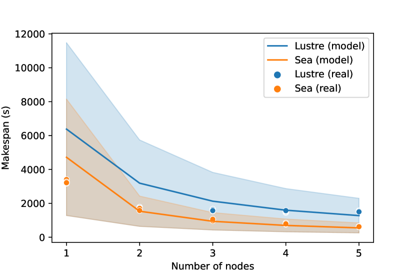
(a) Experiment 1: Varying the number of nodes, 10 iterations

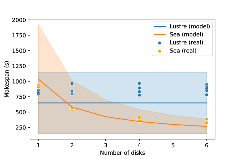
(b) Experiment 2: Varying the number of disks, 5 iterations

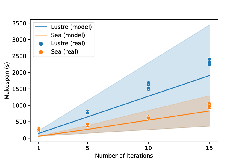
(c) Experiment 3: Varying the number of iterations

(d) Experiment 4: Varying the number of parallel processes, 5 iterations

Figure 2: Benchmarks comparing Lustre and Sea In-memory performance under various conditions using the incrementation application on the Big Brain image. All experiments were repeated 5$\times$. Model bounds represented by coloured regions

4.1 Sea achieves significant speedups

As can be seen in Figure 2, Sea using in-memory configuration speeds up execution the majority of the conditions. The largest speedups observed can be seen in Figure 2(d) at 32 processes, where the speedup is nearly 3$\times$. We believe that the speedup is primarily due to the contention on Lustre. While each local disk has an average of 5 processes trying to write concurrently to it at 32 processes, each Lustre disk has around 3 concurrent processes writing to it. Whereas one might assume this means Lustre would have less contention overall and should perform better, there are significant bandwidth differences to account for between the local disks and Lustre (see Table II) that would result in improved local disk performance despite increased contention. Furthermore, Lustre has a centralized metadata server that is responsible for determining which OST is assigned to each block, guaranteeing a certain amount of load-balance on the storage disks. This is in contrast with the local disks, who do not rely on a metadata server and are selected by Sea via a random shuffling.

The experimental conditions with the next largest speedup can be seen in Figure 2(c) at 10 iterations with a 2.6$\times$ speedup. It is believed that Sea performs best at 10 iterations, rather than 15, because that is when the majority of the writes must be made to local disk. While Sea is not expected to surpass the Lustre makespan, Lustre does have a slight performance advantage in that is able to evict data once it is persisted to Lustre, allowing it to make more efficient use of memory whenever possible.

When varying the number of nodes (Figure 2(a)), we achieved the greatest speedup at 5 nodes, with a speedup of 2.4$\times$. Similar to our experiments with multiprocessing, the speedup appears to be due to increased contention on Lustre. However, there is one main difference, and that is that only Sea is experiencing increased contention, as the contention within the compute nodes is fixed. Both the model and experimental results state that the speedup is approaching a plateau, however, it is expected that once the number of threads writing to Lustre exceeds the number of OSTs (e.g., 9 nodes), we will observe an even greater speedup from Sea due to the increased contention on Lustre.

As expected, our results demonstrate that with an increase in local disk, we can achieve greater speedups. Our results (Figure 2(b)) show that at 6 disks, we achieve a speedup of 2$\times$. This is natural, due to the fact that the most disks we have, the less contention there will be on any given disk. In particular, in our case, each disk at 6 disks should optimally only have a single process writing to it.

When Sea does not provide speedups, it either performs similarly to Lustre, as can be seen in Figure 2(a) at one node and in Figure 2(c) at 1 iteration, or sightly slows down execution, as can be seen in 2(b). As expected, Sea at a single iteration can at best perform similarly or slightly worse than Lustre. This is because all the data is read from Lustre and written to Lustre, operating in the same way that Lustre would with page cache.

Sea at a single node likely performs equivalently to Lustre because Lustre, in this case, has very good bandwidth, having at most 6 concurrent writes to the whole file system. Furthermore, due to the limited number of concurrent writes on Lustre at any given time, Lustre needs to wait less for writes to flush to disk, making better use of available page cache space. Sea’s performance, in contrast, is negatively impacted as there is more data being written to local storage and the combined bandwidth of the local storage is far less superior to that of Lustre’s, due to only having 6 disks available.

The contention on the disk at Sea operation with only a single local disk is likely the cause of the decline in performance in Figure 2(b). As Lustre has significantly less contention on the file system, it is able to exhibit a superior performance to Sea. As we can see, increasing the number of local disks improves Sea’s performance beyond what Lustre can achieve.

4.2 Performance trends described by the model

Figure 2 shows us that our model can describe the performance trends for all but two experiments: Experiment 3 (Figure 2(c)) and Experiment 4 (Figure 2(d)). In Experiment 3, the model incorrectly represents the bounds for 1 iteration. Since, in this case, all the data should be able to fit in page cache for both Sea and Lustre, it is possible that memory bandwidth has been overestimated, resulting in incorrect model predictions.

We believe that Lustre exceeds the model bounds in Experiment 4 due to increased contention on the file system. While our model predicts that the disk bandwidth will be the bottleneck, thus plateauing at 9 parallel processes per node, there are other Lustre bottlenecks that are not included in the model, like the metadata server. We expect that there were too many incoming requests to the server at 30+ parallel processes, that performance declined above model bounds.

Figure 3: Comparison of the different Sea modes with Lustre on the incrementation application processing 1000 Big Brain blocks with 5 nodes, 5 iterations, 6 disks and 6 parallel processes.

4.3 Significant overheads with Flush-all mode

Figure 3 demonstrates the overhead that can be obtained by using flush-all when there is no compute to mask the flushing. Not only is Sea flush-all 3.5$\times$ slower than Sea in-memory, it is 1.3$\times$ slower than Lustre. The reason for it being slower than Lustre is that Sea flush-all does not evict any files and had to copy files from local disk to Lustre, as a result. In contrast, Lustre does not make use of local disk space. It is able to evict data from memory once it is materialized to Lustre. Consequently, Lustre alone does not have the third overhead of writing the data to disk like Sea flush-all does. The performance loss is likely to not have been discernible if we had compute time that matched data transfer time, however, the performance gain might not have been as significant unless we were writing in parallel data that far exceeded page cache space as the application would not have to wait for data to be flushed to Lustre before proceeding.

5 Discussion

5.1 Lightweight data-management library for CLI applications

Through the interception of glibc calls, Sea successfully manages to redirect I/O to the different available storage devices on an HPC cluster. Since Sea is lightweight and requires minimal configuration, it preserves the characteristics that are important to scientific applications.

At minimum, Sea requires the specification of a configuration file for it to work. A user would need to know details on the cluster storage that can be leveraged as well as approximate details on how much data an application execution can produce at any given time. Due to the simplicity of the configuration file, Sea maintains the ease-of-use requirement for scientific applications.

Sea maintains whole files, as produced by the pipeline. In no instance does it modify or alter the data produced by the pipeline. Since there is no risk of Sea modifying the contents of the data, Sea preserves the reproducibility requirement.

The flush-and-evict process may affect overall application parallelism if multiple Sea instances are launched on a given node. If only a single instance of Sea is called on a compute node, there will only be a single flush and evict process. However, if Sea is launched many times on a given node, there will be many flush and evict processes which may interfere with the application compute. However, our results do not indicate that performance is significantly impacted by the presence of a single flush and evict process.

Sea cannot be used with operating systems that are not Linux-based, and therefore, the use of an application with Sea has limited portability. However, Linux-based operating systems are ubiquitous in HPC, and therefore, Sea is not limiting for its intended use case. Furthermore, we provide publicly available containers  to simplify the usage of Sea on various other operating systems.

5.2 In-memory performance with Sea

Our results indicate that Sea can significantly improve the performance in applications executing data-intensive workflows. In all experiments, we observed speedups of up to 3$\times$, with the majority of cases reaching a 2$\times$ speedup. In very few cases did the use of Sea not result in any speedups. In two of the three scenarios, Sea performed identically to Lustre, either because Sea was issuing the same amount of data transfers to Lustre or Lustre bandwidth far exceeded what was available locally.

On shared cluster environments, such as those found in high-performance computing clusters, it is less likely that the PFS would be so underused that it could achieve better performance than leveraging local storage, even if local storage was limited. We therefore believe that it is very unlikely to obtain no speedups from using Sea on a production HPC cluster as long as the application is data intensive.

For our experiments we relied on a synthetic data-intensive application, however, the I/O patterns exhibited by such an application do not adequately mimic the patterns of scientific applications. In our experiments, we demonstrate what the possible performance upper bound can look like and how it is affected by various different factors. Despite the fact that typical scientific workflows may not be as data-intensive, it is believed that scientific applications can still benefit a significant amount by limiting writes to a shared PFS that is experiencing traffic generated by many other users. Furthermore, given that scientific applications have more compute, Sea flush-all can be used with reduced overheads.

5.3 Performance boost with local storage availability

As expected, Sea’s performance increases with the number of disks available. However, our results also demonstrate that it does not require that many disks to surpass Lustre’s performance, even when Lustre is underutilized. Therefore, while Sea underperformed at a single disk, it is likely that this will be sufficient to experience speedups even in a production environment, where Lustre has to deal with user traffic across the cluster. This is important to note because it is not uncommon for HPC cluster compute nodes to only have a single disk available as burst buffer. However, should more disks be available, it would be best to include as many as possible in Sea.

5.4 Sea preferred when Lustre is overloaded

In instances where contention on Lustre exceeds that of local disks, Sea in-memory outperforms Lustre. In all cases, it did not take very much for Sea to outperform Lustre. It is expected that the resource requirements of scientific applications running on HPC systems could far exceed those of our current experiments, relying on 100s of nodes instead of just 5. Therefore, data-intensive scientific applications would benefit greatly from using Sea.

When Lustre is not overloaded, there is little benefit to using Sea. However, we found that Sea performs similarly to Lustre in these cases. Since there is no real penalty to using Sea when Lustre is not overloaded, it is recommended to use Sea in all scenarios. Moreover, users on HPC clusters are unaware of what the PFS performance will be at the time when their experiments will be scheduled. Knowing that Sea does not incur significant overheads will allow users to freely execute Sea without hesitation.

5.5 Flush when necessary and evict often

The results demonstrate that flushing all the data incurs significant overheads with a data-intensive application. These overheads can be so significant that Sea’s performance, in these cases, can be found to be inferior to that of Lustre. In applications where data is shared or when results are required for post-processing, there is no other option than to flush this data. Since the majority of the overhead appears to have arisen from writing to and flushing from local disk, it is recommended that lesser-used data be evicted from Sea, freeing up space for newer data.

There is limited benefit to Sea when flushing all the data in a data-intensive scenario. Sea must perform the same number of I/O operations as Lustre in these cases. While the application itself can proceed to completion faster, as it only needs to wait for all the data to be written to local storage, the time required for the final flush of the data can be quite significant, particularly when flushing from disk to Lustre. Therefore, we recommend that flushing all the data is reserved for more compute-intensive applications.

Increase in performance from eviction is not only limited to scenarios where all the data is flushed. Sea also benefits from eviction when using the in-memory option as not all data may fit in memory and thus need to be written to slower local storage. Sea currently cannot handle scenarios where the application is attempting to access a file that is in the process of being moved, and as a result, we were not able to use much eviction in our experiments. This would be an important feature to enable in future Sea releases, despite the potential slowdown that may be incurred from waiting for the data to be materialized to Lustre.

6 Conclusion

We created Sea, a lightweight open-source data-management library for scientific applications. With the help of glibc interception, we were able to create a library that maintains qualities important to scientific computing (i.e. ease-of-use, reproducibility, portability and parallelism). Our results demonstrate that Sea is quite beneficial to reducing the data transfers overheads, particularly when using an in-memory computing configuration, producing speedups of up to 3$\times$. Sea’s performance is, however, limited when the PFS is not being heavily used.

Experimental results demonstrate that our performance model accurately depicts the bounds in the majority of the cases. The model overestimated performance when metadata calls were heavily impacting performance. This is because the model neglects to account for any kind of latency. More accurate predictions could be obtained with a more complex model, although, due to Lustre’s complex functioning, a simulator would likely be more appropriate here.

More complex functioning of Sea, such as splitting of individual files, as seen with the other burst buffer file systems, may be preferential, particularly in maximizing cache usage. However, the more we complicate these libraries, the harder they are for users to use. As a result, users must wait until the cluster guidelines are developed detailing how a user should use these libraries. The boundary between ease-of-use and performance needs to be further explored to determine what is best for users and applications.

Acknowlegments

Valérie Hayot-Sasson was funded by the Canadian Open Neuroscience Platform (CONP) Scholar Award. This work was also supported by the Canada Foundation for Innovation as well as the Canada Research Chairs program.

Valérie Hayot-Sasson is a PhD student at Concordia University in the Big Data for Neuroinformatics lab. Her research interests focus on studying the effects of data transfers on Big Data scientific application.

Mathieu Dugré is a Ph.D. student at the Big Data Infrastructure for Neuroinformatics lab at Concordia University, Montreal, Canada. His research interests are in Big Data performance techniques for neuroimaging applications.

Tristan Glatard is Associate Professor in the Department of Computer Science and Software Engineering at Concordia University in Montreal, and Canada Research Chair (Tier II) on Big Data Infrastructures for Neuroinformatics. Before that, he was research scientist at the French Na- tional Centre for Scientific Research and Visiting Scholar at McGill University.

References

- [1] Katrin Amunts, Claude Lepage, Louis Borgeat, Hartmut Mohlberg, Timo Dickscheid, Marc-Étienne Rousseau, Sebastian Bludau, Pierre-Louis Bazin, Lindsay B Lewis, Ana-Maria Oros-Peusquens, et al. BigBrain: an ultrahigh-resolution 3D human brain model. Science, 340(6139):1472–1475, 2013.
- [2] Louisa Bessad, Martin Quinson, and Sébastien Monnet. Real-time online emulation of real applications on simgrid with simterpose. 2015.
- [3] Eugenio Cesario, Toni Cortes, Erich Focht, Matthias Hess, Felix Hupfeld, Björn Kolbeck, Jesús Malo, Jonathan Martí, and Jan Stender. The XtreemFS Architecture. Linux Tag, 2007.
- [4] C.S. Daley, D. Ghoshal, G.K. Lockwood, S. Dosanjh, L. Ramakrishnan, and N.J. Wright. Performance characterization of scientific workflows for the optimal use of burst buffers. Future Generation Computer Systems, 110:468–480, 2020.
- [5] Jeffrey Dean and Sanjay Ghemawat. MapReduce: simplified data processing on large clusters. Comm. of the ACM, 51(1):107–113, 2008.
- [6] Oscar Esteban, Christopher J Markiewicz, Ross W Blair, Craig A Moodie, A Ilkay Isik, Asier Erramuzpe, James D Kent, Mathias Goncalves, Elizabeth DuPre, Madeleine Snyder, et al. fmriprep: a robust preprocessing pipeline for functional mri. Nature methods, 16(1):111–116, 2019.
- [7] Dorota Jarecka, Mathias Goncalves, Christopher J Markiewicz, Oscar Esteban, Nicole Lo, Jakub Kaczmarzyk, and Satrajit Ghosh. Pydra-a flexible and lightweight dataflow engine for scientific analyses. In Proceedings of the 19th python in science conference, volume 132, page 139, 2020.
- [8] Sandeep Koranne. Hierarchical data format 5: HDF5. In Handbook of open source tools, pages 191–200. Springer, 2011.
- [9] Haoyuan Li. Alluxio: A virtual distributed file system. PhD thesis, UC Berkeley, 2018.
- [10] Parmita Mehta, Sven Dorkenwald, Dongfang Zhao, Tomer Kaftan, Alvin Cheung, Magdalena Balazinska, Ariel Rokem, Andrew Connolly, Jacob Vanderplas, and Yusra AlSayyad. Comparative evaluation of Big-Data systems on scientific image analytics workloads. Proc. of the VLDB Endowment, 10(11):1226–1237, 2017.
- [11] Alistair Miles, jakirkham, Matthias Bussonnier, Martin Durant, Josh Moore, Andrew Fulton, James Bourbeau, Tarik Onalan, Joe Hamman, Zain Patel, Matthew Rocklin, Ryan Abernathey, Elliott Sales de Andrade, Vincent Schut, raphael dussin, Gregory R. Lee, Charles Noyes, Davis Bennett, shikharsg, Chris Barnes, Aleksandar Jelenak, Anderson Banihirwe, David Baddeley, Eric Younkin, George Sakkis, Ian Hunt-Isaak, Jan Funke, Jerome Kelleher, and Joe Jevnik. zarr-developers/zarr-python: v2.8.3, July 2021.
- [12] Gregory F Pfister. An introduction to the InfiniBand architecture. High performance mass storage and parallel I/O, 42(617-632):102, 2001.
- [13] Matthew Rocklin. Dask: Parallel computation with blocked algorithms and task scheduling. In Proc. of the 14th Python in Science Conference, pages 130–136. Citeseer, 2015.
- [14] Philip Schwan et al. Lustre: Building a file system for 1000-node clusters. In Proc. of the 2003 Linux symposium, volume 2003, pages 380–386, 2003.
- [15] Konstantin Shvachko, Hairong Kuang, Sanjay Radia, and Robert Chansler. The Hadoop distributed file system. In Mass storage systems and technologies (MSST), 2010 IEEE 26th symposium on, pages 1–10. IEEE, 2010.
- [16] Rik Van Riel. Page Replacement in Linux 2.4 Memory Management. In USENIX Annual Technical Conference, FREENIX Track, pages 165–172, 2001.
- [17] Bharath Kumar Reddy Vangoor, Vasily Tarasov, and Erez Zadok. To FUSE or not to FUSE: Performance of user-space file systems. In 15th USENIX Conference on File and Storage Technologies (FAST 17), pages 59–72, 2017.
- [18] Marc-André Vef, Nafiseh Moti, Tim Süß, Tommaso Tocci, Ramon Nou, Alberto Miranda, Toni Cortes, and André Brinkmann. Gekkofs - a temporary distributed file system for hpc applications. In 2018 IEEE International Conference on Cluster Computing (CLUSTER), pages 319–324, 2018.
- [19] Adina S Wagner, Laura K Waite, Małgorzata Wierzba, Felix Hoffstaedter, Alexander Q Waite, Benjamin Poldrack, Simon B Eickhoff, and Michael Hanke. FAIRly big: A framework for computationally reproducible processing of large-scale data. Scientific Data, 9(1):1–17, 2022.
- [20] Teng Wang, Kathryn Mohror, Adam Moody, Kento Sato, and Weikuan Yu. An ephemeral burst-buffer file system for scientific applications. In SC ’16: Proceedings of the International Conference for High Performance Computing, Networking, Storage and Analysis, pages 807–818, 2016.
- [21] Matei Zaharia, Reynold S Xin, Patrick Wendell, Tathagata Das, Michael Armbrust, Ankur Dave, Xiangrui Meng, Josh Rosen, Shivaram Venkataraman, Michael J Franklin, et al. Apache Spark: a unified engine for big data processing. Comm. of the ACM, 59(11):56–65, 2016.