A weak version of Mond’s conjecture

Abstract.

We prove that a map germ $f:(\mathbb{C}^{n},S)\to(\mathbb{C}^{n+1},0)$ with isolated instability is stable if and only if $\mu_{I}(f)=0$, where $\mu_{I}(f)$ is the image Milnor number defined by Mond. In a previous paper we proved this result with the additional assumption that $f$ has corank one. The proof here is also valid for corank $\geq 2$, provided that $(n,n+1)$ are nice dimensions in Mather’s sense (so $\mu_{I}(f)$ is well defined). Our result can be seen as a weak version of a conjecture by Mond, which says that the $\mathscr{A}_{e}$-codimension of $f$ is $\leq\mu_{I}(f)$, with equality if $f$ is weighted homogeneous. As an application, we deduce that the bifurcation set of a versal unfolding of $f$ is a hypersurface.

1. Introduction

In the context of Thom-Mather theory (deformation theory) for map germs $f:(\mathbb{C}^{n},S)\to(\mathbb{C}^{p},0)$, the cases $p<n+1$, $p=n+1$ and $p>n+1$ present different traits and behaviours. In particular, the case $p=n+1$ has several open questions that are understood for the other cases. Here we solve two of them: one regarding the homotopy type of a generic fiber and the other regarding the bifurcation set.

A hypersurface $(X,0)$ with isolated singularity has a well known invariant given by its Milnor fiber, the Milnor number $\mu(X,0)$. D. Mond introduced a similar invariant for map germs $f:(\mathbb{C}^{n},S)\to(\mathbb{C}^{n+1},0)$ with isolated instability in [20]. Indeed, the image of a stable perturbation of $f$ has the homotopy type of a wedge of spheres of dimension $n$, whose number is independent of the stable perturbation. This number of spheres is the image Milnor number of $f$, denoted by $\mu_{I}(f)$, and its stable perturbation plays the role of Milnor fiber of a hypersurface as before. However, this is only well defined when $f$ has corank one or, alternatively, $(n,n+1)$ are nice dimensions in Mather’s sense (cf. [18]).

On the other hand, the $\mathscr{A}_{e}$-codimension of a germ as above is the equivalent of the Tjurina number $\tau(X)$ of a hypersurface with isolated singularity, because they control the space of perturbations of map germs and germs of hypersurfaces, respectively.

The easy relation between the Tjurina and Milnor number for hypersurfaces inspired D. Mond to conjecture in [20] that the relation is reproduced in the case of map germs with isolated instability. More precisely:

Conjecture 1.1 (Mond’s conjecture).

Given a germ $f:(\mathbb{C}^{n},S)\to(\mathbb{C}^{n+1},0)$ with finite $\mathscr{A}_{e}$-codimension such that it has corank one or $(n,n+1)$ are nice dimensions (i.e., $n<15$),

$$\mu_{I}(f)\geq\mathscr{A}_{e}\text{-}\operatorname{codim}(f),$$

with equality in the quasi-homogeneous case.

This question remains open in general (see [4, Theorem 4.2] and [21, Theorem 2.3] for the cases $n=1,2$).

In this paper we show a basic result on both objects of map germs. In Section 2 we deal with the image Milnor number an prove that it is positive if the germ is, indeed, unstable. This is a weak version of 1.1 (i.e., when $\mu_{I}(f)=0$ we have $\mathscr{A}_{e}\text{-}\operatorname{codim}(f)=0$) but it implies this conjecture in the case of $\mathscr{A}_{e}$-codimension one and the case of augmentations of such germs. In order to prove these results we also introduce new objects such as $LC(G)$, a version of Saito’s characteristic variety $LC(\mathcal{X})$, to control the image Milnor number. Furthermore, a deep understanding of $LC(G)$ allows us to prove that, if it is Cohen-Macaulay, Mond’s conjecture is true for germs with a one parameter stable unfolding.

The bifurcation set is the set of parameters of a versal unfolding such that the corresponding perturbations have instabilities. In Section 3 we prove that the bifurcation set of a germ $f:(\mathbb{C}^{n},S)\to(\mathbb{C}^{n+1},0)$ is a pure dimensional hypersurface. Its relevance is also put into perspective by explaining that the methods used to prove a similar fact in other settings fail in our case. Furthermore, a profound understanding of the space of unstable perturbations could lead to a proof of Mond’s conjecture (see the program to solve this conjecture in the first author’s thesis, [8, Section 7.3]). Knowing that the bifurcation set is of codimension one is the first step in that direction.

We refer to the modern reference [22] for the definitions and properties about singularities of mappings such as stability, finite determinacy, versal unfoldings, and other basic concepts.

2. Unstable germs and the image Milnor number

Throughout this section we assume that $f\colon(\mathbb{C}^{n},S)\to(\mathbb{C}^{n+1},0)$ is an $\mathscr{A}$-finite germ such that it has corank one or $(n,n+1)$ are nice dimensions.

We fix a representative $f\colon U\to V$ which is a finite mapping (i.e., finite-to-one and closed) and denote by $X=f(U)$ its image. The germ of $f$ at the point $y\in X$ is denoted by

$$(f)_{y}:\big{(}\mathbb{C}^{n},f^{-1}(y)\big{)}\to(\mathbb{C}^{n+1},y).$$

There is a natural stratification on an $\mathscr{A}$-finite germ $f$, which is straightforward in the case of a stable germ.

Definition 2.1.

Suppose $f$ is stable. The isosingular locus of $f$ at a point $y_{0}$ in the image $X$ is the set

$$\operatorname{Iso}\big{(}f;y_{0}\big{)}\coloneqq\left\{y\in X:(f)_{y}\text{ is }\mathscr{A}\text{-equivalent to }(f)_{y_{0}}\right\}.$$

Moreover, the stratification by stable types of the image of $f$ is given by the isosingular loci of all points $y_{0}\in X$. There is an induced stratification in the source of $f$, these two stratifications are the stratification by stable types of $f$.

We refer to [22, Definition 7.2] for details and properties of this stratification. In fact, the hypothesis that $f$ has corank one or $(n,n+1)$ are in the nice dimensions guarantees that we have a finite number of strata. The name of stable types is taken because, obviously, this stratification identifies stable singularities of the same $\mathscr{A}$-class (cf. Figure 1). Indeed, there is an analogous definition of the stratification by stable types of a locally stable map.

In contrast, it could happen that $f:(\mathbb{C}^{n},S)\rightarrow(\mathbb{C}^{n+1},0)$ has instabilities. However, it has isolated instability if it is $\mathscr{A}$-finite (by Mather-Gaffney criterion). We can assume $f\colon U-S\to V-0$ is locally stable and extend its stratification by stable types just by adding the strata $S$ and $0$ in source and target, respectively. We call this stratification stratification by stable types of $f$ as well (see Figure 1).

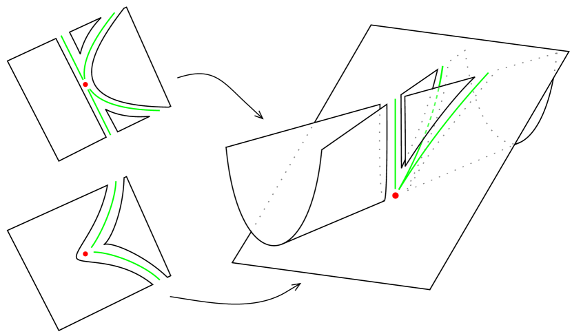
Figure 1. Stratification by stable types of an unstable bigerm given by a crosscap and an immersion. Observe that the transverse double points are in the same stratum.

Let $F(x,s)=(f_{s}(x),s)$ be a stabilisation of $f\colon(\mathbb{C}^{n},S)\to(\mathbb{C}^{n+1},0)$. Then, $F$ is also $\mathscr{A}$-finite, considered as a germ $(\mathbb{C}^{n}\times\mathbb{C},S\times 0)\to(\mathbb{C}^{n+1}\times\mathbb{C},0)$. We denote by $(\mathcal{X},0)$ the image of $F$ in $(\mathbb{C}^{n+1}\times\mathbb{C},0)$ and by $\pi\colon(\mathcal{X},0)\to(\mathbb{C},0)$ the restriction of the projection onto the parameter space. For each $s$ close to $0$ in $\mathbb{C}$, the fibre $\pi^{-1}(s)$ is $X_{s}$, the image of $f_{s}$.

We remark that $F$ still has a well defined stratification by stable types on its image $\mathcal{X}$, although now $(n+1,n+2)$ could be in the boundary of the nice dimensions. In fact, if $(y,s)\in\mathcal{X}-0$, then the germ of $f_{s}$ at $y$ is stable. Therefore, the germ of $F$ at $(y,s)$ is a trivial unfolding of the germ of $f_{s}$ at $y$. Since $(n,n+1)$ are nice dimensions or the germ has corank one, only a finite number of stable types of germs from $\mathbb{C}^{n}$ to $\mathbb{C}^{n+1}$ can appear. Thus, the family of isosingular loci $\operatorname{Iso}\big{(}F;(y,s)\big{)}$ at points $(y,s)\in\mathcal{X}-\{0\}$ is finite. By adding the origin if necessary as a new stratum, we get the stratification by stable types of $\mathcal{X}$ (see Figure 2).

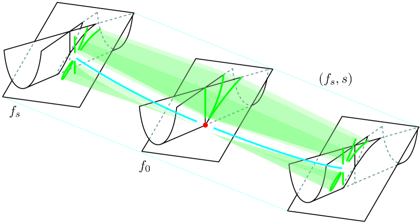
Figure 2. Stratification by stable types of the image of an unfolding $(f_{s},s)$ of the unstable bigerm $f_{0}$ given by a crosscap and an immersion. Observe that, in contrast to Figure 1, the stratum of dimension zero in now stable as a germ from $\mathbb{C}^{3}$ to $\mathbb{C}^{4}$. In a general unfolding this stratum could be unstable.

Lemma 2.2.

The (connected components of the) stratification by stable types of the hypersurface $(\mathcal{X},0)$ coincides with the logarithmic stratification. In particular, $(\mathcal{X},0)$ is holonomic.

Proof.

Given two points $(y,s)$ and $(y^{\prime},s^{\prime})$ in $\mathcal{X}$ in the same connected component of the stratification by stable types, the germs of $F$ at $(y,s)$ and $(y^{\prime},s^{\prime})$ are $\mathscr{A}$-equivalent. In particular, the germs of $\mathcal{X}$ at $(y,s)$ and $(y^{\prime},s^{\prime})$ are equivalent by a biholomorphism $\Psi$ of the ambient space $\mathbb{C}^{n+1}\times\mathbb{C}$. Thus, by connectivity $(y,s)$ and $(y^{\prime},s^{\prime})$ belong to the same stratum in the logarithmic stratification of $\mathcal{X}$.

But the converse also holds. Indeed, the germ $F$ at each point is the normalisation of $\mathcal{X}$ at that point. If the germs of $\mathcal{X}$ at $(y,s)$ and $(y^{\prime},s^{\prime})$ are equivalent by a biholomorphism $\Psi$ of $\mathbb{C}^{n+1}\times\mathbb{C}$, there exists a unique biholomorphism $\Phi$ in $\mathbb{C}^{n}\times\mathbb{C}$ so that $(\Phi,\Psi)$ gives an $\mathscr{A}$-equivalence between the germs of $F$ at $(y,s)$ and $(y^{\prime},s^{\prime})$. Modulo connectivity, this shows that the stratification by stable types coincides with the logarithmic stratification.∎

Lemma 2.3.

The projection $\pi\colon(\mathcal{X},0)\to(\mathbb{C},0)$ has isolated critical points in the stratified sense. Moreover, it has a critical point if, and only if, $f$ is not stable.

Proof.

As above, we fix a representative $\mathcal{X}$ and take $(y,s)\in\mathcal{X}-\{0\}$. Since the germ of $f_{s}$ at $y$ is stable, the germ of $F$ at $(y,s)$ is a trivial unfolding of the germ of $f_{s}$ at $y$. Hence, there exist biholomorphisms $\Phi$ and $\Psi$ in $\mathbb{C}^{n}\times\mathbb{C}$ and $\mathbb{C}^{n+1}\times\mathbb{C}$, respectively, which are unfoldings of the identities and such that $\Psi\circ F\circ\Phi^{-1}=f_{s}\times\operatorname{id}_{\mathbb{C}}$ in a neighbourhood of $(y,s)$. This gives a commutative diagram

$$\leavevmode\hbox to128pt{\vbox to56.64pt{\text{[drawing]}}}, {\big{(}\mathcal{X},(y,s)\big{)}} {(\mathbb{C},s)} {\big{(}X_{s}\times\mathbb{C},(y,s)\big{)}} \scriptstyle{\pi} \scriptstyle{\Psi} \scriptstyle{\sim} \scriptstyle{\pi_{2}} {\big{(}\mathcal{X},(y,s)\big{)}} {(\mathbb{C},s)} {\big{(}X_{s}\times\mathbb{C},(y,s)\big{)}} \scriptstyle{\pi} \scriptstyle{\Psi} \scriptstyle{\sim} \scriptstyle{\pi_{2}}$$

so $(y,s)$ is a regular point of $\pi$ in the stratifed sense.

Assume now that the origin $0$ is also a regular point of $\pi$ in the stratifed sense. Let $S_{0}=\operatorname{Iso}(F;0)$ be the stratum of $\mathcal{X}$ which contains $0$. Obviously, we must have $S_{0}\neq\{0\}$, and since $F$ is stable at any point $(y,s)\in S_{0}-\{0\}$, $F$ is also stable at $0$. As $0\in S_{0}$ is a regular point of the restriction $\pi\colon S_{0}\to\mathbb{C}$, we deduce that the hyperplane $\pi^{-1}(0)=\mathbb{C}^{n+1}\times\{0\}$ is transverse to $S_{0}$. By [23, Proposition 2.22], $f_{0}=f$ is stable at $0$. The converse is obvious, as any unfolding is trivial and has the form $F(x,t)=\big{(}f_{t}(x),t\big{)}$ up to $\mathscr{A}$-equivalence. ∎

Example 2.4.

In Figure 2 we have represented an unfolding $(f_{s},s)$ of the unstable bigerm $f_{0}:\big{(}\mathbb{C}^{2},\left\{p,q\right\}\big{)}\to(\mathbb{C}^{3},0)$ given by a crosscap and an immersion (see also Figure 1), where $f_{s}$ is a stable perturbation of $f_{0}$ (i.e., $(f_{s},s)$ is a stabilisation).

It is easy to see that Lemma 2.3 holds in this case. Indeed, the unique stratum of dimension zero is also the unique critical point of the projection to the parameter $s$.

The fact that this point is stable as a germ induced by the unfolding $(f_{s},s)$ (i.e., as a germ from $\mathbb{C}^{3}$ to $\mathbb{C}^{4}$) plays no role in this fact. In general, if we begin with an unstable $f_{0}$ then, in the unfolding, we need to add as a stratum the point where the instability of $f_{0}$ is located, regardless whether it is stable or unstable as a germ induced by the unfolding.

Let $\theta_{n+2}$ be the $\mathscr{O}_{n+2}$-module of germs of vector fields on $\mathbb{C}^{n+2}\equiv\mathbb{C}^{n+1}\times\mathbb{C}$ at the origin. We denote by $\operatorname{Der}(-\log\mathcal{X})$ the submodule of logarithmic vector fields. We recall that $\xi\in\operatorname{Der}(-\log\mathcal{X})$ if and only if $\xi_{p}\in T_{p}\mathcal{X}$, for all $p\in\mathcal{X}_{reg}$, the regular part of $\mathcal{X}$. Equivalently, $\xi\in\operatorname{Der}(-\log\mathcal{X})$ if and only if $dG(\xi)\in(G)$, where $G\in\mathscr{O}_{n+2}$ such that $G=0$ is a reduced equation of $\mathcal{X}$.

Take a representative $\mathcal{X}$ in some open neighbourhood $U$ of the origin in $\mathbb{C}^{n+2}$. We extend the stratification of $\mathcal{X}$ to $U$ by adding the open stratum $U-\mathcal{X}$. The projection $\pi\colon U\to\mathbb{C}$ has also an isolated stratified critical point at the origin and, hence, the Bruce-Roberts number

$$\mu_{BR}(\mathcal{X},\pi):=\operatorname{dim}_{\mathbb{C}}\frac{\mathscr{O}_{n+2}}{d\pi\big{(}\operatorname{Der}(-\log\mathcal{X})\big{)}}$$

is always finite (see [1, Definition 2.4] and the previous comments) and is not zero when $\pi$ has a critical point at the origin, that is, when $f$ is not stable (by Lemma 2.3). It seems natural to ask about the relationship between this number and $\mu_{I}(f)$, which gives the number of vanishing cycles of the fiber $X_{s}=\pi^{-1}(s)$. However, the following example shows that these two numbers are not equal in general.

Example 2.5.

Let $f\colon(\mathbb{C}^{2},0)\to(\mathbb{C}^{3},0)$ be given by $f(x,y)=(x^{2},y^{2},xy+x^{3}+y^{3})$ with stabilisation

$$F(x,y,s)=(x^{2}+sy,y^{2}-sx,xy+y^{3}+x^{3}+s(x-y),s).$$

We have $\mu_{I}(f)=7$ (see [17, Section 3.1]) and a computation with Singular (see [5]) gives that $\mu_{BR}(\mathcal{X},\pi)=8$.

Instead of $\operatorname{Der}(-\log\mathcal{X})$ we will consider the submodule $\operatorname{Der}(-\log G)$, defined as the set of vector fields $\xi$ such that $dG(\xi)=0$. Roughly speaking, the difference between these modules is disregarding the fiber $G^{-1}(0)=\mathcal{X}$ as special and considering the tangency at every fiber of $G$. Obviously, we have the inclusion $\operatorname{Der}(-\log G)\subset\operatorname{Der}(-\log\mathcal{X})$. Moreover, when $\mathcal{X}$ is weighted homogeneous, we also have that

(1) $$\operatorname{Der}(-\log\mathcal{X})=\operatorname{Der}(-\log G)\oplus\mathscr{O}_{n+2}\cdot\{\epsilon\},$$

where $\epsilon$ is the Euler vector field

$$\epsilon=w_{1}\frac{\partial}{\partial x_{1}}+\cdots+w_{n+1}\frac{\partial}{\partial x_{n+1}}+w_{s}\frac{\partial}{\partial s},$$

$w_{\bullet}$ denoting the corresponding weights of the variables. Moreover, since $d\pi(\epsilon)=w_{s}s$, we obtain the equality

(2) $$d\pi\big{(}\operatorname{Der}(-\log\mathcal{X})\big{)}=d\pi\big{(}\operatorname{Der}(-\log G)\big{)}+(s).$$

The ideal $d\pi\big{(}\operatorname{Der}(-\log G)\big{)}\subset\mathscr{O}_{n+2}$ contains relevant information we want to analyse. Observe that if, at a point $p$, the tangent space of the fiber of $G(p)$ coincides with the tangent space of the fiber of $\pi(p)$, i.e., if

$$T_{p}G^{-1}\big{(}G(p)\big{)}=T_{p}\pi^{-1}\big{(}\pi(p)\big{)},$$

then $p$ will be in the set of zeros of $d\pi\left(\operatorname{Der}(-\log G)\right)\subset\mathscr{O}_{n+2}$ (see Figure 3). Hence, at least, this ideal contains the information of the failure of the transversality between the fibers of $\pi$ and $G$. For this reason, we use the notation

$$FT(\pi,G)\coloneqq d\pi\big{(}\operatorname{Der}(-\log G)\big{)}.$$

Note, however, that if we consider the points where the fibers of $G$ are not smooth this does not work, so $FT(\pi,G)$ refines this notion.

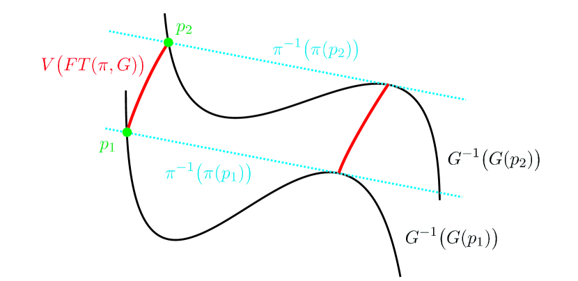
Figure 3. Representation of the set of zeros of the ideal $FT(\pi,G)=d\pi\big{(}\operatorname{Der}(-\log G)\big{)}$. Observe that it has two components in this representation.

In the following lemma, we consider the general case where $\mathcal{X}$ is not necessarily weighted homogeneous. For each $s\in\mathbb{C}$ close enough to the origin, we denote by $g_{s}$ the function $g_{s}(y)=G(y,s)$.

Lemma 2.6.

The zero locus $V\big{(}FT(\pi,G)\big{)}$ of $FT(\pi,G)$ in $(\mathbb{C}^{n+2},0)$ is the set-germ of points $(y,s)$ such that either:

1. $(y,s)=0$ and $f$ is not stable, or

2. $G(y,s)\neq 0$ and $y$ is a critical point of $g_{s}$.

Moreover, in the second case, $FT(\pi,G)$ is generated by $\frac{\partial G}{\partial y_{1}},\dots,\frac{\partial G}{\partial y_{n+1}}$ in a neighbourhood of $(y,s)$.

Proof.

By the curve selection lemma, $G$ has isolated critical value at the origin. We fix a representative in some open neighbourhood $U$ of the origin in $\mathbb{C}^{n+2}$ such that $f_{s}$ is stable at $y$, for all $(y,s)\in\mathcal{X}-\{0\}$ and $0$ is the only critical value of $G$.

Let $p=(y_{0},s_{0})\in U$. We first consider the case $G(p)=0$, so $p\in\mathcal{X}$.

If $f_{s_{0}}$ is stable at $y_{0}$ (in particular, if $p\neq 0$), then $p$ is not a critical point of $\pi\colon U\to\mathbb{C}$, by Lemma 2.3. Hence, $p\notin V\big{(}d\pi\big{(}\operatorname{Der}(-\log\mathcal{X})\big{)}\big{)}$. On the other hand, at $p$, $F$ is a trivial unfolding of the germ $(f_{s_{0}})_{y_{0}}$, as it is stable. Since we deal with corank one germs or $(n,n+1)$ are nice dimensions, the germ $(f_{s_{0}})_{y_{0}}$ is weighted homogeneous, up to $\mathscr{A}$-equivalence (see [22, Theorem 7.6]). In particular, $\mathcal{X}$ is weighted homogeneous in a neighbourhood of $p$, up to a coordinate change which preserves the parameter $s$. It follows from Equation 2 that

$$d\pi\big{(}\operatorname{Der}(-\log\mathcal{X})\big{)}=d\pi\big{(}\operatorname{Der}(-\log G)\big{)}+(s-s_{0})=FT(\pi,G)+(s-s_{0}),$$

in a neighbourhood of $p$. Hence, $p\notin V\big{(}FT(\pi,G)\big{)}$ because $p\in V(s-s_{0})$.

If $p=0$ and $f$ is unstable at that point, then $0$ is a critical point of $\pi\colon U\to\mathbb{C}$ (by Lemma 2.3) and, hence,

$$0\in V(d\pi\big{(}\operatorname{Der}(-\log\mathcal{X})\big{)}\subset V\big{(}FT(\pi,G)\big{)}.$$

Now we consider the case $G(p)\neq 0$. By assumption, $G$ is regular at $p$. Assume that $\frac{\partial G}{\partial y_{i}}(p)\neq 0$, for some $i=1,\dots,n+1$. We can suppose, for simplicity, that $i=1$. The map

$$\Phi(y,s)=\big{(}G(y,s),y_{2},\dots,y_{n+1},s\big{)}$$

is a biholomorphism in a neighbourhood of $p$ and

$$G\circ\Phi^{-1}(z,y_{2}\dots,y_{n+1},s)=z,$$

in a neighbourhood of $\Phi(p)$. The module $\operatorname{Der}\big{(}-\log(G\circ\Phi^{-1})\big{)}$ is generated at $\Phi(p)$ by the vector fields $\frac{\partial}{\partial y_{2}},\dots,\frac{\partial}{\partial y_{n+1}},\frac{\partial}{\partial s}$. Composing by the differential of $\Phi$ we reverse the coordinate change, so $\operatorname{Der}(-\log G)$ is generated at $p$ by

$$\hskip 56.9055pt\xi_{i} =\frac{\partial}{\partial y_{i}}+\frac{\partial G}{\partial y_{i}}\frac{\partial}{\partial y_{1}},\quad i=2,\dots,n+1,$$

$$\xi_{n+2} =\frac{\partial}{\partial s}+\frac{\partial G}{\partial s}\frac{\partial}{\partial y_{1}}.$$

We have $d\pi(\xi_{n+2})=1$, so $p\notin V\big{(}FT(\pi,G)\big{)}$.

The case $\frac{\partial G}{\partial s}(p)\neq 0$ has to be analysed separately. We proceed analogously and arrive to that $\operatorname{Der}(-\log G)$ is generated at $p$ by

$$\eta_{i}=\frac{\partial}{\partial y_{i}}+\frac{\partial G}{\partial y_{i}}\frac{\partial}{\partial s},\quad i=1,\dots,n+1.$$

In this case $d\pi(\eta_{i})=\frac{\partial G}{\partial y_{i}}$. Hence, $FT(\pi,G)$ is generated at $p$ by $\frac{\partial G}{\partial y_{1}},\dots,\frac{\partial G}{\partial y_{n+1}}$, and $p\in V\big{(}FT(\pi,G)\big{)}$ if and only if $y_{0}$ is a critical point of $g_{s_{0}}$. ∎

Corollary 2.7.

The number

$$\operatorname{dim}_{\mathbb{C}}\frac{\mathscr{O}_{n+2}}{FT(\pi,G)+(s)}$$

is always finite and is not zero if and only if $f$ is not stable.

Proof.

By shrinking the neighbourhood $U$ if necessary, we can assume that $0$ is the only critical value of $g_{0}$. Hence, by Lemma 2.6, we have that

$$V\big{(}FT(\pi,G)+(s)\big{)}\subset\{0\},$$

with equality if and only if $f$ is not stable. The results follows now from the analytic Nullstellensatz. ∎

Example 2.8.

In Example 2.5, we have

$$\operatorname{dim}_{\mathbb{C}}\frac{\mathscr{O}_{n+2}}{FT(\pi,G)+(s)}=7,$$

which coincides with $\mu_{I}(f)$.

In the next theorem, we consider $\mathscr{O}_{n+2}/FT(\pi,G)$ as an $\mathscr{O}_{1}$-module via the morphism $\pi^{*}\colon\mathscr{O}_{1}\to\mathscr{O}_{n+2}$. By Corollary 2.7, $\mathscr{O}_{n+2}/FT(\pi,G)$ is always finitely generated over $\mathscr{O}_{1}$.

Theorem 2.9.

The image Milnor number of $f$ equals the Samuel multiplicity of $\mathscr{O}_{n+2}/FT(\pi,G)$ with respect to the maximal ideal $(s)$, i.e.,

$$\mu_{I}(f)=e\left((s);\frac{\mathscr{O}_{n+2}}{FT(\pi,G)}\right).$$

Proof.

Take $s_{0}\neq 0$ close enough to the origin in $\mathbb{C}$. By the conservation of the multiplicity (see, for example, [22, Corollary E.5]),

$$e\left((s);\frac{\mathscr{O}_{n+2}}{FT(\pi,G)}\right) =\sum_{(y,s_{0})\in V(FT(\pi,G))}e\left((s-s_{0});\frac{\mathscr{O}_{n+2,(y,s_{0})}}{FT(\pi,G)}\right)$$

$$=\sum_{(y,s_{0})\in V(FT(\pi,G))}e\left((s-s_{0});\frac{\mathscr{O}_{n+2,(y,s_{0})}}{\left(\frac{\partial G}{\partial y_{1}},\dots,\frac{\partial G}{\partial y_{n+1}}\right)}\right)$$

$$=\sum_{y\notin X_{s_{0}}}\operatorname{dim}_{\mathbb{C}}\frac{\mathscr{O}_{n+1,y}}{\left(\frac{\partial g_{s_{0}}}{\partial y_{1}},\dots,\frac{\partial g_{s_{0}}}{\partial y_{n+1}}\right)}$$

$$=\sum_{y\notin X_{s_{0}}}\mu(g_{s_{0}};y)$$

$$=\mu_{I}(f).$$

The second equality follows from Lemma 2.6, the third one holds because

$$\frac{\mathscr{O}_{n+2,(y,s_{0})}}{\left(\frac{\partial G}{\partial y_{1}},\dots,\frac{\partial G}{\partial y_{n+1}}\right)}$$

is Cohen-Macaulay, and the last one is a consequence of a theorem due to Siersma, [25, Theorem 2.3]. ∎

Remark 2.10.

The multiplicity $e\left((s);\frac{\mathscr{O}_{n+2}}{FT(\pi,G)}\right)$ can be interpreted geometrically as a local intersection number

$$e\left((s);\frac{\mathscr{O}_{n+2}}{FT(\pi,G)}\right)=i\left(j,V\big{(}FT(\pi,G)\big{)}\right),$$

where $j\colon(\mathbb{C}^{n+1},0)\to(\mathbb{C}^{n+2},0)$ is the embedding $y\mapsto(y,0)$. We refer to Fulton’s book [7] for details about the connection between the algebraic multiplicity and the local intersection number.

An alternative explanation of this equality can be given as we know that the points of $V\big{(}FT(\pi,G)\big{)}$ are precisely the instability of $f_{0}$ and the critical points of $g_{s}$, where $g_{s}$ is the equation of $\operatorname{Im}(f_{s})$, that are not contained in the image of $f_{s}$, by Lemma 2.6. Moreover, we have already mentioned that a result of Siersma (see [25, Theorem 2.3]) says that the sum of the Milnor numbers of these critical points is equal to the image Milnor number of $f_{0}$. In other words,

$$\sum_{y\notin X_{s_{0}}}\mu(g_{s_{0}};y)=\mu_{I}(f),$$

which is equal to the intersection multiplicity $i\big{(}j,V\big{(}FT(\pi,G)\big{)}\big{)}$ and, in turn, equal to the Samuel multiplicity $e\big{(}(s);\frac{\mathscr{O}_{n+2}}{FT(\pi,G)}\big{)}$ (by Theorem 2.9 above). See Remarks 2.15 and 4 below.

Corollary 2.11.

In terms of Theorem 2.9,

$$\mu_{I}(f)\leq\operatorname{dim}_{\mathbb{C}}\frac{\mathscr{O}_{n+2}}{FT(\pi,G)+(s)},$$

with equality if and only if $\mathscr{O}_{n+2}/FT(\pi,G)$ is Cohen-Macaulay of dimension $1$.

The following definition is an adaptation of the definition of the logarithmic characteristic variety $LC(\mathcal{X})$ introduced by Saito in [24], where we consider the module $\operatorname{Der}(-\log G)$ instead of $\operatorname{Der}(-\log\mathcal{X})$.

Let $T^{*}\mathbb{C}^{n+2}$ be the cotangent bundle of $\mathbb{C}^{n+2}$. Given an open set $U\subset\mathbb{C}^{n+2}$, $T_{U}^{*}\mathbb{C}^{n+2}$ is the restriction of $T^{*}\mathbb{C}^{n+2}$ to $U$. An element of $T_{U}^{*}\mathbb{C}^{n+2}$ will be of the form $(y,s;\alpha)$, where $(y,s)\in U$ and $\alpha\colon\mathbb{C}^{n+2}\to\mathbb{C}$ is a linear form.

Given a holomorphic function $h\colon U\to\mathbb{C}$ (or a germ $h\colon(\mathbb{C}^{n+2},0)\to\mathbb{C}$), we denote by $Dh\colon U\to T^{*}\mathbb{C}^{n+2}$ (resp. $Dh\colon(\mathbb{C}^{n+2},0)\to T^{*}\mathbb{C}^{n+2}$) the differential, that is, the section of $T^{*}\mathbb{C}^{n+2}$ given by $Dh(y,s)=\big{(}y,s;dh_{(y,s)}\big{)}$.

Definition 2.12.

Assume that $\xi_{1},\dots,\xi_{r}$ generate $\operatorname{Der}(-\log G)$ on some open neighbourhood $U$ of the origin in $\mathbb{C}^{n+2}$. Then, the logarithmic characteristic variety of $G$ is defined as follows:

$$LC_{U}(G)=\left\{(y,s;\alpha)\in T_{U}^{*}\mathbb{C}^{n+2}:\ \alpha(\xi_{i}(y,s))=0,\ \forall i=1,\dots,r\right\}.$$

The variety $LC(G)$ is the germ of $LC_{U}(G)$ along $T_{0}^{*}\mathbb{C}^{n+2}$.

It is easy to see that

(3) $$D\pi^{-1}\big{(}LC(G)\big{)}=V\big{(}FT(\pi,G)\big{)}.$$

To give the equations of $LC(G)$, suppose that the module $\operatorname{Der}(-\log G)$ is generated by germs of vector fields $\xi_{1},\dots,\xi_{r}$ and that

$$\xi_{i}=\sum_{i=1}^{n+1}a_{j}^{i}\frac{\partial}{\partial y_{j}}+b_{i}\frac{\partial}{\partial s},$$

for some $a_{j}^{i},b_{i}\in\mathscr{O}_{n+2}$. Denote by $(y_{1},\dots,y_{n+1},s,p_{1},\dots,p_{n+1},q)$ the coordinates of $T^{*}\mathbb{C}^{n+2}$. Then $LC(G)$ has equations $\xi^{*}_{i}=0$, $i=1,\dots,r$, where

$$\xi_{i}^{*}=\sum_{i=1}^{n+1}a_{j}^{i}p_{j}+b_{i}q\in\mathscr{O}_{n+2}[p_{1},\dots,p_{n+1},q].$$

This shows that $LC(G)$ is independent of the choice of the neighbourhood $U$. It is not difficult to see that it is also independent of the choice of the generators. We remark that $LC(G)$ is considered with the possibly non-reduced structure given by the ideal generated by $\xi^{*}_{i}$, $i=1,\dots,r$.

We know that $LC(\mathcal{X})$ has dimension $n+2$, for $(\mathcal{X},0)$ is holonomic (see [1, Proposition 1.14]). We compute the dimension of $LC(G)$ in the next proposition.

Proposition 2.13.

The variety $LC(G)$ has dimension $n+3$. Furthermore, the variety $V\big{(}FT(\pi,G)\big{)}$ has dimension $1$ if, and only if, $f$ is not stable and is empty otherwise.

Proof.

By Corollary 2.7,

$$\operatorname{dim}_{\mathbb{C}}\frac{\mathscr{O}_{n+2}}{FT(\pi,G)+(s)}<\infty,$$

so $\operatorname{codim}V\big{(}FT(\pi,G)\big{)}\geq n+1$, and, by Equation 3, $\operatorname{codim}LC(G)\geq n+1$. Hence, $\operatorname{dim}V\big{(}FT(\pi,G)\big{)}\leq 1$ and $\operatorname{dim}LC(G)\leq n+3$.

On the other hand, $G$ has isolated critical value at the origin by the curve selection Lemma. We take a small enough open neighbourhood $U$ of the origin in $\mathbb{C}^{n+2}$ such that $0$ is the only critical value of $G$ on $U$. For each $(y,s)\in U-\mathcal{X}$, $G$ is regular at $(y,s)$. We use the argument given in the proof of Lemma 2.6 and deduce that $\operatorname{Der}(-\log G)$ is generated in a neighbourhood of $(y,s)$ by $n+1$ vector fields $\xi_{1},\dots,\xi_{n+1}$. It follows that $LC(G)$ is given in a neighbourhood of $(y,s)$ by $n+1$ equations $\xi^{*}_{i}=0$, $i=1,\dots,n+1$, so $\operatorname{codim}LC(G)\leq n+1$. Hence, $\operatorname{dim}LC(G)=n+3$ and $\operatorname{dim}V\big{(}FT(\pi,G)\big{)}=1$ whenever it is not empty. However, by Corollary 2.7, $FT(\pi,G)$ contains the constants if, and only if, $f$ is stable, and $V\big{(}FT(\pi,G)\big{)}$ would be empty. ∎

Now we prove a weak version of Mond’s conjecture 1.1 for the case $\mu_{I}(f)=0$. This is a generalization of [9, Theorem 3.9], which is stated for corank one germs.

Theorem 2.14.

We have that $\mu_{I}(f)=0$ if and only if $f$ is stable.

Proof.

Assume that $f$ is not stable. We know from Proposition 2.13 that $\operatorname{dim}LC(G)=n+3$ and $\operatorname{dim}V\big{(}FT(\pi,G)\big{)}=1$. In other words,

$$\operatorname{dim}\mathscr{O}_{n+2}/FT(\pi,G)=1=\operatorname{dim}\mathscr{O}_{1}$$

and, hence,

$$\mu_{I}(f)=e\left((s);\frac{\mathscr{O}_{n+2}}{FT(\pi,G)}\right)\geq 1,$$

(see, for instance, [19, Formula 14.2]). ∎

Remark 2.15.

There is an equivalent way of proving this result using the geometry of $V\big{(}FT(\pi,G)\big{)}$. On one hand, we know that

$$\mu_{I}(f)=i\left(j,V\big{(}FT(\pi,G)\big{)}\right),$$

as shown in Remark 2.10. On the other, this intersection number is positive, because $V\big{(}FT(\pi,G)\big{)}$ is curve (see Proposition 2.13), so the result follows. See Figure 4 for a general overview of this reasoning.

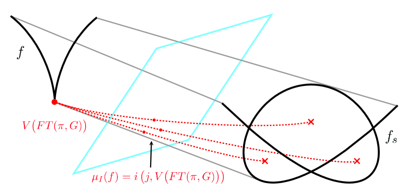
Figure 4. The curve $V\big{(}FT(\pi,G)\big{)}$ and the intersection number $i\left(j,V\big{(}FT(\pi,G)\big{)}\right)$.

Corollary 2.16.

Mond’s conjecture is true for germs of $\mathscr{A}_{e}$-codimension 1 (see 1.1).

Proof.

The general case follows from Theorem 2.14. If $f$ is quasi-homogeneus then its $\mathscr{A}_{e}$-codimension coincides with the dimension as vector space of the Jacobian module $M(g)$, see [6], hence

$$0<\mu_{I}(f)\leq\operatorname{dim}_{\mathbb{C}}M(g)=1,$$

by [6, Proof of Theorem 6.1]. ∎

Cooper, Mond and Wik Atique proved this result for corank one germs in [2, Theorem 7.2]. Actually, they proved that, in corank one, germs with $\mathscr{A}_{e}$-codimension 1 have image Milnor number equal to 1. This fact led Houston to prove that Mond’s conjecture holds for a class of germs called augmentations of corank one germs that have $\mathscr{A}_{e}$-codimension one (see [14, Corollary 6.8]). We can generalize the proof to germs of any corank using the same ideas. The concept of augmentation was first introduced in [11], and the reader can find its definition in, for example, [13, Definition 3.1].

Corollary 2.17.

Suppose that $A_{F,g}(f)$ is an augmentation with $g$ of a germ $f:(\mathbb{C}^{n},S)\rightarrow(\mathbb{C}^{n+1},0)$ of $\mathscr{A}_{e}$-codimension one. If $f$ or $g$ are quasi-homogeneous, $A_{F,g}(f)$ satisfies Mond’s conjecture and, more precisely,

$$\mathscr{A}_{e}\text{-}\operatorname{codim}\big{(}A_{F,g}(f)\big{)}=\mathscr{A}_{e}\text{-}\operatorname{codim}(f)\tau(g)\leq\mu_{I}(f)\mu(g)=\mu_{I}\big{(}A_{F,g}(f)\big{)},$$

where $\tau$ denotes the Tjurina number, with equality if $f$ and $g$ are quasi-homogeneous.

Proof.

The result is a consequence of Corollary 2.16 and [14, Theorem 6.7] (see also [13, Theorem 3.3], which controls the $\mathscr{A}_{e}$-codimension of augmentations). There is, however, a small consideration to be made: the equality

$$\mu(g)\mu_{I}(f)=\mu_{I}\big{(}A_{F,g}(f)\big{)}$$

is stated for corank one monogerms in [14, Corollary 6.4]. One can give the same proof for multigerms of any corank, using the well known fact that the image of a stable perturbation of any $f$ with our hypothesis has the homotopy type of a wedge of spheres (see, for example, [22, Proposition 8.3]). ∎

Theorem 2.18.

Let $f:(\mathbb{C}^{n},S)\to(\mathbb{C}^{n+1})$ be a germ such that $(n,n+1)$ are nice dimensions or it has corank one. Then,

$$\mu_{I}(f)=i\big{(}D\pi\circ j,LC(G)\big{)},$$

where $j(y)=(y,0)$, as in Remark 2.10.

Proof.

In fact, we have

$$i\big{(}D\pi\circ j,LC(G)\big{)}=e\left(\mathfrak{m}_{n+3,(0,\pi)};\mathscr{O}_{LC(G),D\pi(0)}\right),$$

where we consider $\mathscr{O}_{LC(G),D\pi(0)}$ as a module over $\mathscr{O}_{n+3,(0,\pi)}$ via the projection $T^{*}\mathbb{C}^{n+2}\to\mathbb{C}\times\mathbb{C}^{n+2}=\mathbb{C}^{n+3}$ given by $(y,s;\alpha)\mapsto(s;\alpha)$.

As in the proof of Theorem 2.9 we use the conservation of the multiplicity (see, for example, [22, Corollary E.5]). For $(s_{0};\pi)$ with $s_{0}\neq 0$,

$$e\left(\mathfrak{m}_{n+3,(0,d\pi)};\mathscr{O}_{LC(G),D\pi(0)}\right)=\sum_{D\pi(y,s_{0})\in LC(G)}e\left(\mathfrak{m}_{n+3,(s_{0},\pi)};\mathscr{O}_{LC(G),D\pi(y,s_{0})}\right).$$

Since $G$ is regular at each $(y,s_{0})$, $\operatorname{Der}(-\log G)$ is generated by $n+1$ vector fields at $(y,s_{0})$, therefore $LC(G)$ is given by $n+1$ equations at $D\pi(y,s_{0})$. So, $LC(G)$ is Cohen-Macaulay at $D\pi(y,s_{0})$ and, hence,

$$e\left(\mathfrak{m}_{n+3,(s_{0},\pi)};\mathscr{O}_{LC(G),D\pi(y,s_{0})}\right) =\operatorname{dim}_{\mathbb{C}}\frac{\mathscr{O}_{LC(G),D\pi(y,s_{0})}}{\mathfrak{m}_{n+3,(s_{0},\pi)}\mathscr{O}_{LC(G),D\pi(y,s_{0})}}$$

$$=\operatorname{dim}_{\mathbb{C}}\frac{\mathscr{O}_{V(FT(\pi,G)),(y,s_{0})}}{\mathfrak{m}_{1,s_{0}}\mathscr{O}_{V(FT(\pi,G)),(y,s_{0})}}$$

$$=\operatorname{dim}_{\mathbb{C}}\frac{\mathscr{O}_{n+2,(y,s_{0})}}{FT(\pi,G)+\mathfrak{m}_{1,s_{0}}}$$

$$=\mu(g_{s_{0}};y);$$

where the last equality is given by Lemma 2.6.

Using [25, Theorem 2.3] as in Theorem 2.9, this shows that

$$e\left(\mathfrak{m}_{n+3,(0,\pi)};\mathscr{O}_{LC(G),{D\pi}(0)}\right)=\mu_{I}(f),$$

and the result follows. ∎

Observe that, as we are using multiplicities in the proof of Theorem 2.18, the equality

$$\mu_{I}(f)=\operatorname{dim}_{\mathbb{C}}\frac{\mathscr{O}_{n+2}}{FT(\pi,G)+(s)},$$

holds if and only if $LC(G)$ is Cohen-Macaulay at $(0,\pi)$. This leads to the following result.

Theorem 2.19.

Mond’s conjecture is true for germs $f$ with one parameter stable unfoldings $F$ (OPSU) and such that $LC(G)$ is Cohen-Macaulay, for $G$ given by $F$ (see 1.1).

Proof.

As we were saying, we have conservation of the multiplicity, since $LC(G)$ is Cohen-Macaulay, so

(4) $$\mu_{I}(f)=\operatorname{dim}_{\mathbb{C}}\frac{\mathscr{O}_{n+1}}{FT(\pi,G)+(s)}.$$

Now, by [22, Theorem 8.7] (see the original version in [3]),

$$T^{1}\mathscr{A}_{e}(f)\cong\frac{\theta(i)}{ti(\theta_{n+1})+i^{*}\big{(}\operatorname{Der}(-\log\mathcal{X})\big{)}},$$

where $i$ is given by the commutative diagram

$$\leavevmode\hbox to160.7pt{\vbox to55.01pt{\text{[drawing]}}}, {(\mathbb{C}^{n}\times\mathbb{C},S\times\left\{0\right\})} {(\mathbb{C}^{n+1}\times\mathbb{C},0)} {(\mathbb{C}^{n},S)} {(\mathbb{C}^{n+1},0)} \scriptstyle{F} \scriptstyle{f} \scriptstyle{j} \scriptstyle{i} {(\mathbb{C}^{n}\times\mathbb{C},S\times\left\{0\right\})} {(\mathbb{C}^{n+1}\times\mathbb{C},0)} {(\mathbb{C}^{n},S)} {(\mathbb{C}^{n+1},0)} \scriptstyle{F} \scriptstyle{f} \scriptstyle{j} \scriptstyle{i}$$

and $i$ is transverse to $F$. However, we can do the identifications $\theta(i)/di(\theta_{Y})\cong\theta(\pi)/\mathfrak{m}_{1}\theta(\pi)$ and $\theta(\pi)\cong\mathscr{O}_{n+1}$, so

(5) $$T^{1}\mathscr{A}_{e}(f) \cong\frac{\theta(\pi)}{d\pi\big{(}\operatorname{Der}(-\log\mathcal{X})\big{)}+\mathfrak{m}_{1}\theta(\pi)}$$

$$\cong\frac{\mathscr{O}_{n+1}}{d\pi\big{(}\operatorname{Der}(-\log\mathcal{X})\big{)}+(s)}.$$

Recall that, by definition, $FT(G,\pi)=d\pi\big{(}\operatorname{Der}(-\log G)\big{)}$, and the decomposition

$$d\pi\big{(}\operatorname{Der}(-\log\mathcal{X})\big{)}=d\pi\big{(}\operatorname{Der}(-\log G)\big{)}+(s)$$

in the quasi-homogeneous case given in Equation 2. Hence, comparing Equations 4 and 5, the result follows. ∎

3. Bifurcation set

In this section we prove that the bifurcation set of an $\mathscr{A}$-finite germ $f:(\mathbb{C}^{n},S)\rightarrow(\mathbb{C}^{n+1},0)$ is a hypersurface that has pure dimension. This is, indeed, the only case where it is not known whether the bifurcation set is a hypersurface (without any additional hypotheses).

For germs $f:(\mathbb{C}^{n},S)\rightarrow(\mathbb{C}^{p},0)$ with $n\geq p$, this property is shown in [22, Theorem 8.8], whose proof relies on the fact that the discriminant is a free divisor in this case (see [16, Corollary 6.13], cf. [22, Proposition 8.9]). This is no longer true for $p>n$.For germs with $p\geq n+2$ the bifurcation set can have greater codimension, see [22, Example 9.5]. Finally, when $p=n+1$, it was only known that the bifurcation set is a hypersurface for germs of corank one (see [22, Proposition 9.15]). This, in turn, relied in the good structure of the multiple point spaces, which lose this good behaviour when we study germs with greater corank.

Consider a map germ $f:(\mathbb{C}^{n},S)\to(\mathbb{C}^{n+1},0)$ with $\mathscr{A}_{e}$-codimension $d>0$ and a miniversal unfolding (see Figure 5)

$$F:\big{(}\mathbb{C}^{n}\times\mathbb{C}^{d},S\times\{0\}\big{)} \to(\mathbb{C}^{n+1}\times\mathbb{C}^{d},0)$$

$$(x,\lambda) \mapsto\big{(}f_{\lambda}(x),\lambda\big{)}.$$

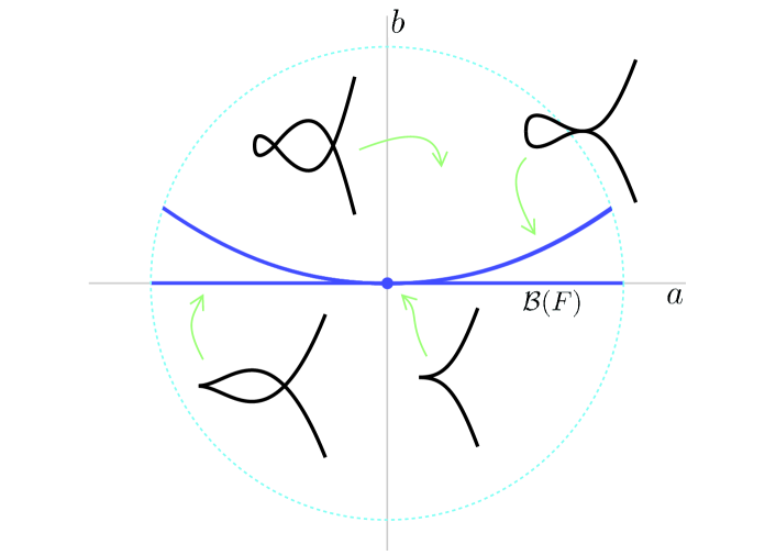
Figure 5. Representation of the parameter space of the miniversal unfolding $F(x,a,b)=(x^{2},x^{5}+ax^{3}+bx,a,b)$ of $f(x)=(x^{2},x^{5})$.

We want to use some ideas Goryunov used in [12] to reach a version for more dimensions of his [12, Corollary] given for germs from $\mathbb{C}^{2}$ to $\mathbb{C}^{3}$. Indeed, it is implicit in Goryunov’s work the result given here as Theorem 2.14 or, as it is proven in those dimensions, Mond’s conjecture (see [4, Theorem 4.2] and [21, Theorem 2.3]).

We can consider a generic line $\tilde{\ell}$ in $\mathbb{C}^{d}$ through the origin to compute the multiplicity of the bifurcation set $\mathscr{B}(F)$. Hence, when we shift the line $\tilde{\ell}$ to the new line $\ell$, the number $\nu$ of points in $\ell\cap\mathscr{B}(F)$ is the multiplicity of $\mathscr{B}(F)$ at the origin. Observe, however, that this multiplicity is positive if, and only if, $\mathscr{B}(F)$ is a hypersurface and, to prove that it is positive, we will use Theorem 2.14.

We can consider the pullback $F^{\ell}$ induced by $\ell$ and $F$, i.e., $F^{\ell}(x,t)\coloneqq\big{(}f_{\ell(t)}(x),t\big{)}$ where $\ell(t)$ parametrizes the line $\ell$. Notice that this is a deformation of the pullback $F^{\tilde{\ell}}$ induced by $\tilde{\ell}$ and $F$.

Theorem 3.1.

If $f$ has corank one or it is in the nice dimensions, the bifurcation set $\mathscr{B}(F)$ is a hypersurface.

Proof.

We are going to use stratified Morse theory with a function induced from the projection $\pi$ to the parameter $\lambda$ in the image of $F^{\ell}$:

$$\leavevmode\hbox to109.3pt{\vbox to38.96pt{\text{[drawing]}}}, {\phi:\operatorname{Im}F^{\ell}} {\ell} {\big{(}f_{\ell(t)}(x),t\big{)}} {\left|\ell(t)-q_{0}\right|} {\phi:\operatorname{Im}F^{\ell}} {\ell} {\big{(}f_{\ell(t)}(x),t\big{)}} {\left|\ell(t)-q_{0}\right|}$$

where $q_{0}$ is a generic point of $\ell$, which can be considered to lie in $\ell-\mathscr{B}(F)$. We also use the stratification given by the stable types (and the isolated unstable points) of $F^{\ell}$.

Observe that a critical point of $\pi$ induces a critical point of $\phi$. Furthermore, the points $p_{i}$ of the intersection $\ell\cap\mathscr{B}(F)$ are, precisely, the critical points of $\pi$ by Lemma 2.3 (or, to be more precise, a very easy adaptation of this result to $F^{\ell}$). By contradiction, if the intersection $\ell\cap\mathscr{B}(F)$ were empty, there would be no critical points, and, by Morse theory, the image of $F^{\ell}$ would be a deformation retract of the image of $f_{q_{0}}$. But this is absurd. Indeed, $F^{\ell}$ is a deformation of $F^{\tilde{\ell}}$, and $f_{q_{0}}$ is a stable perturbation of $f$ (so it has the homotopy type of a wedge of $\mu_{I}(f)$ spheres of dimension $n$). As $f$ has an instability, the number $\mu_{I}(f)$ is positive (by Theorem 2.14), but the image of $F^{\ell}$ has only non-trivial homology in dimension zero and, possibly, in dimension $n+1$. ∎

With these ideas, we can refine the result.

Theorem 3.2.

In the conditions of Theorem 3.1,

$$m\big{(}\mathscr{B}(F)\big{)}\leq\mu_{I}(f)+\mu_{I}\big{(}F^{\tilde{\ell}}\big{)}.$$

Proof.

Using the exact sequence of the pair,

$$0\to H_{n+1}\big{(}\operatorname{Im}F^{\ell}\big{)}\to H_{n+1}\big{(}\operatorname{Im}F^{\ell},\operatorname{Im}f_{q_{0}}\big{)}\to H_{n}(f_{q_{0}})\to 0,$$

we only need to confirm that each point $p_{i}$ (i.e., each critical point of $\pi$) contributes with at least one copy of $\mathbb{Z}$ to $H_{n+1}\big{(}\operatorname{Im}F^{\ell},\operatorname{Im}f_{q_{0}}\big{)}$. Indeed, if $\phi$ is not a stratified Morse function we can consider a Morsification, which has at least one critical point for each critical point of $\phi$ (hence $\pi$). As these images are analytic and $\phi$ is the module of a complex analytic function, the tangential Morse data is

$$(D^{m},\partial D^{m}),$$

where $m$ is the dimension of the stratum that contains the critical point. Furthermore, as we deal with hypersurfaces, a theorem of Lê (see [15], but also the more easy to access [10, pp. 187-188]) says that the normal Morse data is homotopic to

$$\left(\vee D^{n+1-m},\partial\vee D^{n+1-m}\right).$$

Hence, the Morse data is

$$(D^{m},\partial D^{m}) \times\left(\vee D^{n+1-m};\partial\vee D^{n+1-m}\right)$$

$$=\left(D^{m}\times\vee D^{n+1-m};\partial D^{m}\times\vee D^{n+1-m}\cup D^{m}\times\partial\vee D^{n+1-m}\right)$$

$$\simeq\left(\vee D^{n+1};C_{<n+1}\right),$$

where $C_{<n+1}$ is a $CW$-complex of dimension lower than $n+1$. The result follows from here, counting the new cells per critical point. ∎

Proposition 3.3.

In the conditions of Theorem 3.1, the bifurcation set is pure dimensional.

Proof.

By contradiction, assume that $\mathscr{B}(F)$, with reduced structure, has a component that is not a hypersurface. We can consider a point $\lambda$ that lies in that component but not in the other components. By the openness of versality (see [26, Theorem 3.7], cf. [22, Theorem 5.6]), $F$ is also a versal unfolding of $f_{\lambda}$ at each point. This is already a contradiction, as it is not a hypersurface. ∎

Remark 3.4.

It is important to notice that the bifurcation set considered with the reduced structure is not, in general, irreducible. Indeed, in most cases it will have more than one irreducible component (see, for example, [22, Example 5.8]).

References

[1]
J. W. Bruce and R. M. Roberts.
Critical points of functions on analytic varieties.
Topology. An International Journal of Mathematics,
27(1):57–90, 1988.
[2]
T. Cooper, D. Mond, and R. Wik Atique.
Vanishing topology of codimension 1 multi-germs over and
.
Compositio Mathematica, 131(2):121–160, 2002.
[3]
James Damon.
-equivalence and the equivalence of sections of
images and discriminants.
In Singularity theory and its applications, Part I
(Coventry, 1988/1989), volume 1462 of Lecture Notes in Math., pages
93–121. Springer, Berlin, 1991.
[4]
T. de Jong and D. van Straten.
Disentanglements.
In Singularity theory and its applications, Part I
(Coventry, 1988/1989), volume 1462 of Lecture Notes in Math., pages
199–211. Springer, Berlin, 1991.
[5]
Wolfram Decker, Gert-Martin Greuel, Gerhard Pfister, and Hans Schönemann.
Singular 4-2-1 — A computer algebra system for polynomial
computations.
http://www.singular.uni-kl.de, 2021.
[6]
J. Fernández de Bobadilla, J. J. Nuño Ballesteros, and G. Peñafort
Sanchis.
A Jacobian module for disentanglements and applications to Mond’s
conjecture.
Revista Matemática Complutense, 32(2):395–418, 2019.
[7]
William Fulton.
Intersection theory, volume 2 of Ergebnisse der Mathematik
und ihrer Grenzgebiete. 3. Folge. A Series of Modern Surveys in Mathematics
[Results in Mathematics and Related Areas. 3rd Series. A Series of Modern
Surveys in Mathematics].
Springer-Verlag, Berlin, second edition, 1998.
[8]
R. Giménez Conejero.
Singularities of germs and vanishing homology.
PhD thesis, Universitat de València, 2021.
[9]
R. Giménez Conejero and J. J. Nuño-Ballesteros.