The work of Hugo Duminil-Copin

Abstract

The past decade has seen tremendous progress in our understanding of the behaviour of many probabilistic models at or near their “critical point”. On the 5th of July 2022, Hugo Duminil-Copin was awarded the Fields medal for the crucial role he played in many of these developments. In this short review article, we will try to put his work into context and present a small selection of his results.

1 Introduction

Hugo Duminil-Copin was awarded the Fields medal in Helsinki during the opening ceremony of the 2022 virtual ICM. In this short note, I will try to put his work into context and to give the reader a glimpse of why the questions it addresses are not only very interesting from a purely mathematical perspective, but also contribute to further our understanding of nature at a fundamental level. I should start first of all with a disclaimer. Hugo Duminil-Copin is an astounding problem solver and, while his interest falls squarely into the general area of probability theory and in particular the type of probabilistic problems that arise when studying microscopic models for statistical mechanics, I will not be able to do justice to the breadth of his contributions. Furthermore, my own area of expertise is somewhat tangential to that of Duminil-Copin, so this note should be taken as the point of view of an interested outsider. In particular, any misrepresentations of his results and /or techniques will be entirely due to my own ignorance.

In its broadest form, classical statistical mechanics can be thought of as the study of the global behaviour of “large” systems (of “size” $N\gg 1$) that are comprised of many identical “small” subsystems interacting with each other. One typically indexes the subsystems by a discrete set $\Lambda_{N}$ with $\lim_{N\to\infty}|\Lambda_{N}|=\infty$ and one is interested in quantities that are stable as $N\to\infty$. In many cases of interest, one has $\Lambda_{N}\subset\Lambda$ for $\Lambda$ a discrete subset of Euclidean space (typically a regular lattice) and its elements are interpreted as a physical location of the corresponding subsystem; the interaction between subsystems may then depend on their locations. (In most models they actually depend only on their relative positions, a notion that generalises very well to locations taking values in more general symmetric spaces.)

Let us write $S$ for the state space of one single such subsystem, so that the state space for the full system is $\mathcal{S}_{N}\stackrel{{\scriptstyle\mbox{\tiny{def}}}}{{=}}S^{\Lambda_{N}}$. In equilibrium statistical mechanics, we furthermore assume that $S$ is equipped with a “reference” probability measure $\mu$ (think of $\mu$ as being normalised counting measure if $S$ is a finite set, normalised volume measure if it is a compact manifold, etc) and that our system is described by an energy function $H^{(N)}\colon\mathcal{S}_{N}\to\mathbf{R}$, which is typically comprised of a contribution for each subsystem, as well as additional interaction terms. In full generality, one would have something like [e:generalH] H^(N)(σ) = ∑_A ⊂S_N H_A(σ_A) , where $\sigma_{A}$ denotes the restriction of $\sigma\in S^{\Lambda_{N}}$ to $S^{A}$ and the function $H_{A}$ typically only depends on the “shape” of the subset $A$, so satisfies natural invariance properties under translations and possibly reflections and / or discrete rotations. In many classical models, the only non-vanishing terms in (LABEL:e:generalH) are those with $|A|\leq 2$.

Given such an energy function, we obtain a probability measure $\mu_{\beta,N}$ on $\mathcal{S}_{N}$ by setting [e:Gibbs] μ_β,N(dσ) = Z_β,N^-1 exp(- βH^(N)(σ)) ∏_u ∈Λ_Nμ(dσ_u) , where $Z_{\beta,N}$ is chosen in such a way that $\mu_{\beta,N}(\mathcal{S}_{N})=1$. Physically, the parameter $\beta>0$ appearing in this expression is the inverse of the temperature of the system. To a large extent, (equilibrium) statistical mechanics is the study of $\mu_{\beta,N}$ as $N\to\infty$ with a particular emphasis on the behaviour under $\mu_{\beta,N}$ of observables that take a “macroscopic” (of the order of the size of the domain $\Lambda_{N}$) or “mesoscopic” (tending to infinity as $N\to\infty$ but much smaller than $|\Lambda_{N}|$) number of components of $\sigma$ into account.

1.1 Bernoulli percolation

The simplest such example is that of $S=\{-1,1\}$, $H_{N}=0$, and $\mu(\{-1\})=\mu(\{1\})=\frac{1}{2}$. Regarding the index set $\Lambda_{N}$, we consider the case of the even elements of a large box in $\mathbf{Z}^{2}$, namely $\Lambda_{N}=\{u\in\{-N,\ldots,N\}^{2}\,:\,u_{1}+u_{2}\,\mathrm{even}\}$. (The reason why we make this strange choice rather than simply taking all elements of $\{-N,\ldots,N\}^{2}$ will soon become clear.)

One of the simplest kind of “global” observables for this system is given by the following kind of linear statistics. Given a smooth function $\phi\colon[-1,1]^{2}\to\mathbf{R}$, we define $I_{\phi}^{N}\colon\mathcal{S}_{N}\to\mathbf{R}$ by [e:localAverages] I_ϕ^N(σ) = N^-α ∑_u ∈Λ_N σ_u ϕ(u/N) . Note that this is exhaustive: for any fixed $N$, if we know $I_{\phi}^{N}(\sigma)$ for every smooth function $\phi$, then we can in principle recover the argument $\sigma$ itself. A version of the central limit theorem then immediately yields the following result:

Theorem 1.1.

Setting $\alpha=1$, the joint distribution of $I_{\phi}^{N}(\sigma)$ for any finite collection of test functions $\phi$ as above converges as $N\to\infty$ to the law of a collection of jointly centred Gaussian random variables $I_{\phi}$ such that EI_ϕ  I_ψ= 12∫_[-1,1]^2 ϕ(x)ψ(x) dx . (The factor $\frac{1}{2}$ appearing here comes from the fact that the local density of $\Lambda_{N}$ in $\mathbf{Z}^{2}$ is $\frac{1}{2}$.)

A much more interesting kind of global observables is given by the connectivity properties of $\sigma$, which were first studied by Broadbent and Hammersley [Percolation]. These are however much harder to analyse and, even though the model just described appears at first sight to be somewhat trivial, most of its results already lead us squarely into 21st century mathematics. In order to describe what we mean by “connectivity” in this context, instead of interpreting elements $u\in\Lambda_{N}$ as points in $\mathbf{Z}^{2}$, we interpret them as nearest-neighbour edges of a suitable sublattice of $\mathbf{Z}^{2}$ by associating to $u$ the unique edge $e_{u}$ of $\mathbf{Z}_{\mathrm{even}}\times\mathbf{Z}_{\mathrm{odd}}$ with midpoint $u$. We will also write $e_{u}^{*}$ for the edge of $\mathbf{Z}_{\mathrm{odd}}\times\mathbf{Z}_{\mathrm{even}}$ with midpoint $u$. In other words, we set e_u = {(u_↓, u_↑)if $u_{1}$ is even,(u_←, u_→)if $u_{1}$ is odd,  e_u^* = {(u_←, u_→)if $u_{1}$ is even,(u_↓, u_↑)if $u_{1}$ is odd. Here, given $u=(u_{1},u_{2})\in\mathbf{Z}^{2}$, we write $u_{\leftarrow}=(u_{1}-1,u_{2})$, etc. The endpoints of these edges do belong to the stated sublattices of $\mathbf{Z}^{2}$ since $u_{1}+u_{2}$ is even, so either both $u_{1}$ and $u_{2}$ are even or both are odd.

Given a configuration $\sigma\in\mathcal{S}_{N}$, we interpret edges $e_{u}$ with $\sigma_{u}=-1$ as “open” and draw them in black, while the remaining edges are considered “closed” and are drawn in light grey. This yields a picture like shown on the left in Figure 1. We can then ask for example what is the probability $p_{N}$ that it is possible to go from the left boundary of the light gray graph to the right boundary (the "boundary" here consists of the ends of the dangling edges) while only traversing black edges. It turns out that this probability does take non-trivial values even for large values for $N$. As a matter of fact, it is independent of $N$ as the following classical result (see for example [Grimmett, Lem. 11.21]) shows.

Figure 1: On the left, we draw a typical percolation configuration for $N=11$. On the right, the same configuration is drawn together with its dual configuration in light blue.

Theorem 1.2.

One has $p_{N}=\frac{1}{2}$ for every $N$.

Proof.

The trick is to observe that given a configuration $\sigma\in\mathcal{S}_{N}$, if we draw the dual configuration $\sigma^{*}\in\mathcal{S}_{N}$ defined by $\sigma^{*}_{u}=-\sigma_{u}$ by colouring (in blue, say) the edges $e^{*}_{u}$ with $\sigma^{*}_{u}=-1$, then we obtain a drawing with the property that blue edges never intersect black edges. As a consequence, it is possible to cross the square from left to right by traversing only black edges if and only if it is not possible to cross it from top to bottom by traversing only blue edges. (See Figure 1.) On the other hand, the law of the collection of blue edges is the same as that of the collection of black edges, only rotated by $90^{\circ}$, so that we must have $p_{N}=1-p_{N}$ as claimed. ∎

Remark 1.3.

If, instead of choosing edges to be open with probability $\frac{1}{2}$, we choose them to be open with some probability $p$, then we have $p_{N}\to 1$ for $p>\frac{1}{2}$ and $p_{N}\to 0$ for $p<\frac{1}{2}$. This is an example of phase transition: an abrupt change in the behaviour of some global observables as a parameter of the model is varied continuously. In this specific example, we were able to determine the critical value $p_{c}=\frac{1}{2}$ explicitly by exploiting an exact duality.

It is similarly possible to obtain a large collection of interesting global observables by taking a shape $\mathcal{U}\subset[-1,1]^{2}$ diffeomorphic to a square and considering the analogous event $A_{\mathcal{U}}^{(N)}\subset\mathcal{S}_{N}$ asking whether it is possible to connect the left and right edges of $N\mathcal{U}$ (without ever leaving $N\mathcal{U}$) by a path following only open edges of a given configuration $\sigma\in\mathcal{S}_{N}$. Again, the knowledge of these events is an exhaustive statistics for any given fixed value of $N$. It is furthermore known that for any finite number of such shapes $\{\mathcal{U}_{i}\}_{i\in I}$ (for $I$ some finite index set) the random variables $\{[A_{\mathcal{U}_{i}}^{(N)}]\}_{i\in I}$ converge in law to a non-degenerate limit $\{[A_{\mathcal{U}_{i}}]\}_{i\in I}$ as $N\to\infty$ [Stas]. (Here, we write $[A]$ for the indicator function of an event $A$.) An amazing fact is that this scaling limit is conformally invariant: if $\phi\colon D\to D^{\prime}$ is a conformal map between two smooth simply connected domains $D,D^{\prime}\subset\mathbf{C}$ such that $[-1,1]^{2}\subset D$ and such that $\mathcal{V}_{i}\stackrel{{\scriptstyle\mbox{\tiny{def}}}}{{=}}\phi(\mathcal{U}_{i})\subset[-1,1]^{2}$, then the joint law of the random variables $\{[A_{\mathcal{V}_{i}}]\}_{i\in I}$ is the same as that of $\{[A_{\mathcal{U}_{i}}]\}_{i\in I}$.

This conformal invariance turns out to be a crucial feature of the scaling limits of many equilibrium statistical mechanics models in two dimensions. It provides a link to conformal field theory which, at a purely mathematical level, can be thought of as the study of irreducible representations of the Virasoro algebra. In particular, it strongly suggests that the possible large-scale behaviours one can see for two-dimensional equilibrium models come in a one-parameter family of “universality classes” parametrised by the central charge of the corresponding conformal field theory. (In the case of percolation, it turns out that this central charge is given by $c=0$.)

1.2 The Ising model

The next-“simplest” model of statistical mechanics falling into the category of equilibrium models described above is the Ising model [Lenz, Ising]. (See also the review article [HugoICM] in these proceedings which contains a more detailed account of the various developments spawned by this model.) In this case, the index set is given by $\Lambda_{N}=\{-N,\ldots,N\}^{d}$ for some $d\geq 1$, the reference measure $\mu$ and local state space $S$ are as above, but this time one has $H_{A}=0$ unless $A=\{u,v\}$ with $u,v\in\mathbf{Z}^{d}$ such that $|u-v|=1$, in which case one sets $H_{A}(\sigma)=-\sigma_{u}\sigma_{v}$. This time, the model has a non-trivial dependence on the parameter $\beta$ appearing in (LABEL:e:Gibbs), which plays a role somewhat similar to the parameter $p$ that appeared in Remark 1.3.

At a very qualitative level, the situation is somewhat similar to what happened in the case for percolation: in every dimension $d\geq 2$ there exists a critical (dimension-dependent) value $\beta_{c}$ which delineates two different regimes. At “high temperature”, namely for $\beta<\beta_{c}$, the spontaneous magnetisation, namely the random quantity $N^{-d}\sum_{i\in\Lambda_{N}}\sigma_{i}$, converges to $0$ in probability as $N\to\infty$. For $\beta>\beta_{c}$ on the other hand, it converges in probability to a limiting random variable that can take exactly two possible values $\pm h_{\beta}\neq 0$ with equal probabilities. The actual value of $\beta_{c}$ is only known in dimension $2$ where it equals $\beta_{c}=\log\sqrt{1+\sqrt{2}}$ [Onsager]. (There is no phase transition at all in dimension $1$ and the spontaneous magnetisation always vanishes, so in some sense $\beta_{c}=+\infty$ there.)

It is again possible to ask the same questions as in the case of Bernoulli percolation. This time however even the analogue of Theorem 1.1, which was an essentially trivial consequence of the central limit theorem (or at least a version thereof), is already highly non-trivial. It was shown in a recent series of works [Ising2, Ising3] that if one chooses $\beta=\beta_{c}$ and $\alpha=15/8$ in the expression (LABEL:e:localAverages) in dimension $d=2$, then it converges in law to non-trivial limiting random variables, jointly for any fixed number of test functions. This time however the limiting distributions are not Gaussian (they actually exhibit an even faster decaying tail behaviour). Note that the exponent $\alpha$ is closely related to the behaviour of $\mathbf{E}_{c}\sigma_{u}\sigma_{v}$ (where $\mathbf{E}_{c}$ denotes the expectation under the Gibbs measure (LABEL:e:Gibbs) for the critical value of the inverse temperature $\beta$) since, assuming that $\mathbf{E}_{c}\sigma_{u}\sigma_{v}\approx|u-v|^{-\delta}$, one finds that E_c (I_ϕ^N(σ))^2 = N^-2α ∑_u,v ϕ(u/N)ϕ(v/N) E_c σ_u σ_v ≲N^-2α ∑_u,v |u-v|^-δ ≈N^2d - (δ∧d) -2α , so that one expects the relation $\alpha=d-(\delta\wedge d)/2$, which (correctly) leads to the prediction $\delta=\frac{1}{4}$. This and a number of other properties of the Ising model at criticality allow to associate it to the conformal field theory with central charge $c=\frac{1}{2}$.

The picture in higher dimensions is much less clear however. For $d\geq 5$, it was shown in [Triv1, Triv2, Triv3] that the correct scaling exponent to use in (LABEL:e:localAverages) at $\beta=\beta_{c}$ is $\alpha=1+\frac{d}{2}$ and that the limit is a Gaussian Free Field, namely the Gaussian random distribution with correlation function given by the Green’s function of the Laplacian (with Neuman boundary conditions on the square). In dimension $d=3$, virtually nothing is known rigorously about the critical Ising model, not even the value of its scaling exponents, although much progress has been made at a non-rigorous level with the development of the “conformal bootstrap” [Bootstrap1, Bootstrap2]. Regarding the case $d=4$, it was somewhat unclear until very recently whether the Ising model at criticality should be “trivial” (i.e. described by Gaussian distributions) or not. This was eventually settled by Aizenman and Duminil-Copin in the work [Phi44] where they show that any subsequential limit for expressions of the form (LABEL:e:localAverages) as $N\to\infty$ (and $\beta\to\beta_{c}$) must necessarily be Gaussian.

In fact, some of the results just mentioned are shown for the “lattice $\Phi^{4}$ model” which is the equilibrium model with $S=\mathbf{R}$, as well as H_{u}(σ) = V(σ_u) =defσ_u^4 - ασ_u^2 ,  H_{u,v}(σ) = 12 (σ_u - σ_v)^2 , again provided that $u$ and $v$ are nearest-neighbours, and with $c$ an additional parameter. While this appears to be very different from the Ising model at first sight, we can see that it is actually a generalisation of it: if the constant $\alpha$ is large, then the potential $V$ has two very deep wells with minima located at $\pm\sqrt{\alpha}$, so its effect is to impose that $\sigma_{u}\approx\pm\sqrt{\alpha}$ with high probability. The main contribution then comes from the cross-term of the square in the two-body term which is the same as for the Ising model. These kind of considerations lead one to expect that, since these models exhibit long-range correlations at the critical temperature (in the sense that the correlation $\mathbf{E}\sigma_{x}\sigma_{y}$ decays slowly in $|x-y|$ as already pointed out earlier) which should furthermore lead to some form of self-averaging, the Ising model and the $\Phi^{4}$ model exhibit the same behaviour at criticality.

1.3 A general picture

The general picture that should by now be emerging from our discussion can be summarised as follows:

1. Many of the simplest local equilibrium systems do exhibit a phase transition, namely there exists a critical value $\beta_{c}$ at which the qualitative large scale behaviour of the system changes abruptly. In general, a system may depend on additional parameters in which case one may see a more complicated phase diagram with several regions in parameter space where the global behaviour of the system displays qualitatively different behaviour. In any case, the “high temperature / small $\beta$ phase” is expected to behave in such a way that what happens in well separated regions of space is very close to independent.

2. In dimension $2$, many of these systems appear to exhibit a form of conformal invariance at criticality, even though no rotation symmetry is built a priori into their description. When this happens, the link to $2d$ conformal field theories (and the associated probabilistic objects like SLE [SLE], QLE [QLE], etc) provides a hugely powerful machinery to predict –and in a number of cases also rigorously prove –their behaviour.

3. The universe of local statistical mechanics models can be subdivided into broad classes of models that exhibit a shared large-scale behaviour at criticality. These are called “universality classes” and, in the $2d$ equilibrium case, they are expected to come in families parametrised by a real parameter, the central charge. (For certain values of the central charge, one expects to have several “subclasses”, but we will not discuss this kind of subtlety here.)

4. Although one still expects conformal invariance at criticality in higher dimensions, this is a much smaller symmetry there and therefore appears to provide somewhat less insight. One also expects the situation there to be more rigid than in two dimensions, with fewer universality classes. (Possibly only a discrete family.)

5. Models that have “obvious” variants in every dimension typically have a critical dimension above which their behaviour at criticality is “trivial” in the sense that it exhibits Gaussian behaviour. (Typically with correlation function given by the Green’s function of the Laplacian.) In the case of the Ising universality class, this critical dimension is $4$, while in the case of Bernoulli percolation it is $6$.

One important branch of modern probability theory aims to put this general picture onto rigorous mathematical footing. The remainder of this article is devoted to a short overview of some of Hugo Duminil-Copin’s many contributions to this vast programme. This represents of course a mere sliver of his work and completely ignores very substantial chunks of it. By presenting not just a long laundry list of results that he proved and conjectures that he settled but instead an overview of the strategy of proof for a few select results, I hope to be able to convey one of the features of Duminil-Copin’s body of work, namely that he has a knack for finding just the right way of looking at a problem that had hitherto been overlooked. In many cases, this only provides small cracks in the problem’s armour that still require tremendous technical skill to be wedged open, but in some cases it results in surprisingly simple but ingenious proofs. Either way, I am very much looking forward to learning more from Duminil-Copin’s insights for many years to come.

2 (Dis)continuity of phase transitions

One very natural question in this area is whether one can take the limit $N\to\infty$ in (LABEL:e:Gibbs). At this stage, we note that the definition of $H^{(N)}$ given in (LABEL:e:generalH) is not necessarily the most natural one since it restricts the sum over those clusters $A$ that are constrained to entirely lie in $S_{N}$. Another possibility that appears just as natural would be to restrict the sum over clusters that merely intersect $S_{N}$, but to specify some fixed “boundary condition” $\bar{\sigma}\in S^{\Lambda}$ that is used to compute the values of the $H_{A}$ with $A$ intersecting both $\Lambda_{N}$ and $\Lambda\setminus\Lambda_{N}$ in the sense that we interpret $\sigma_{A}$ in (LABEL:e:generalH) as $\sigma_{A,x}=\sigma_{x}$ for $x\in A\cap\Lambda_{N}$ and $\sigma_{A,x}=\bar{\sigma}_{x}$ otherwise.

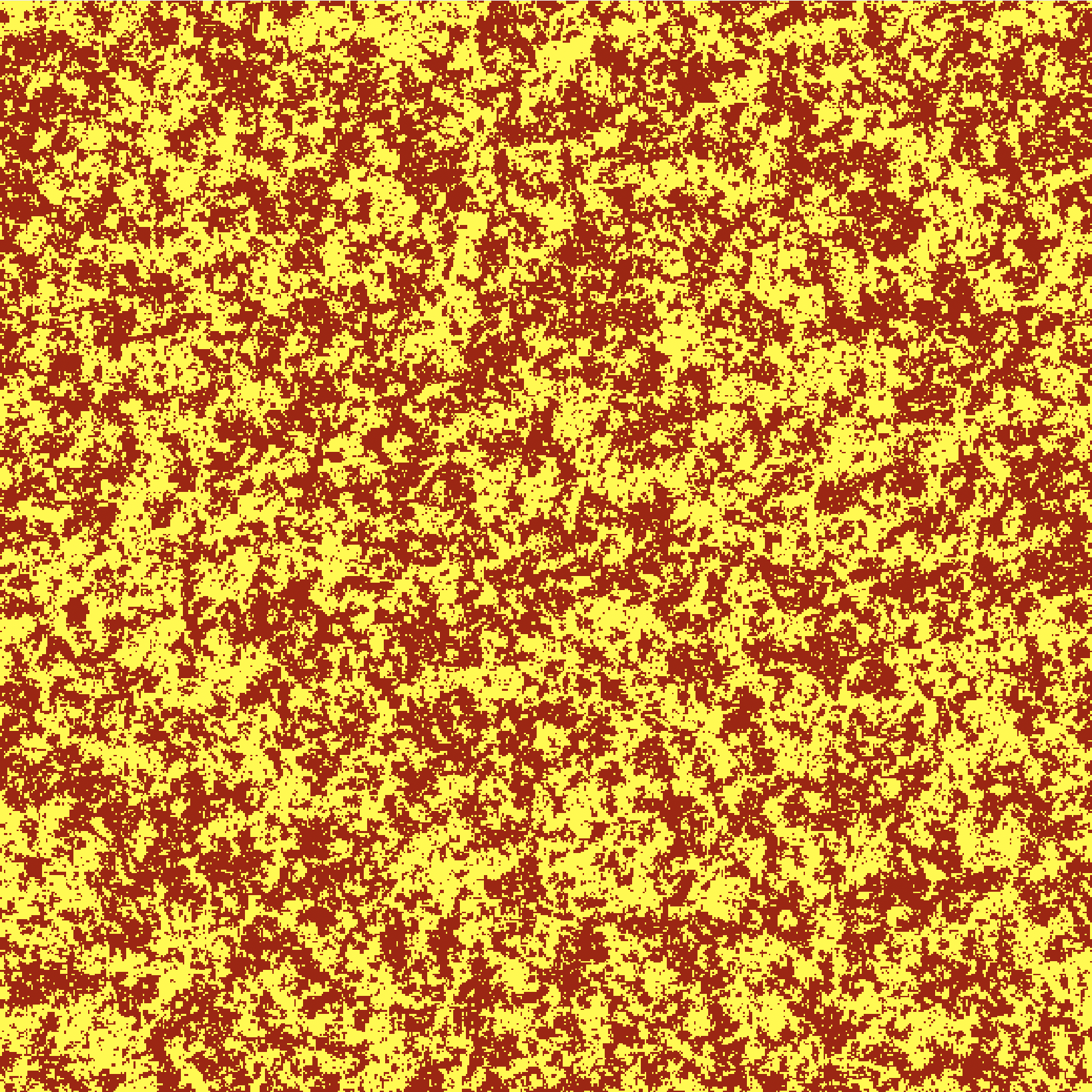
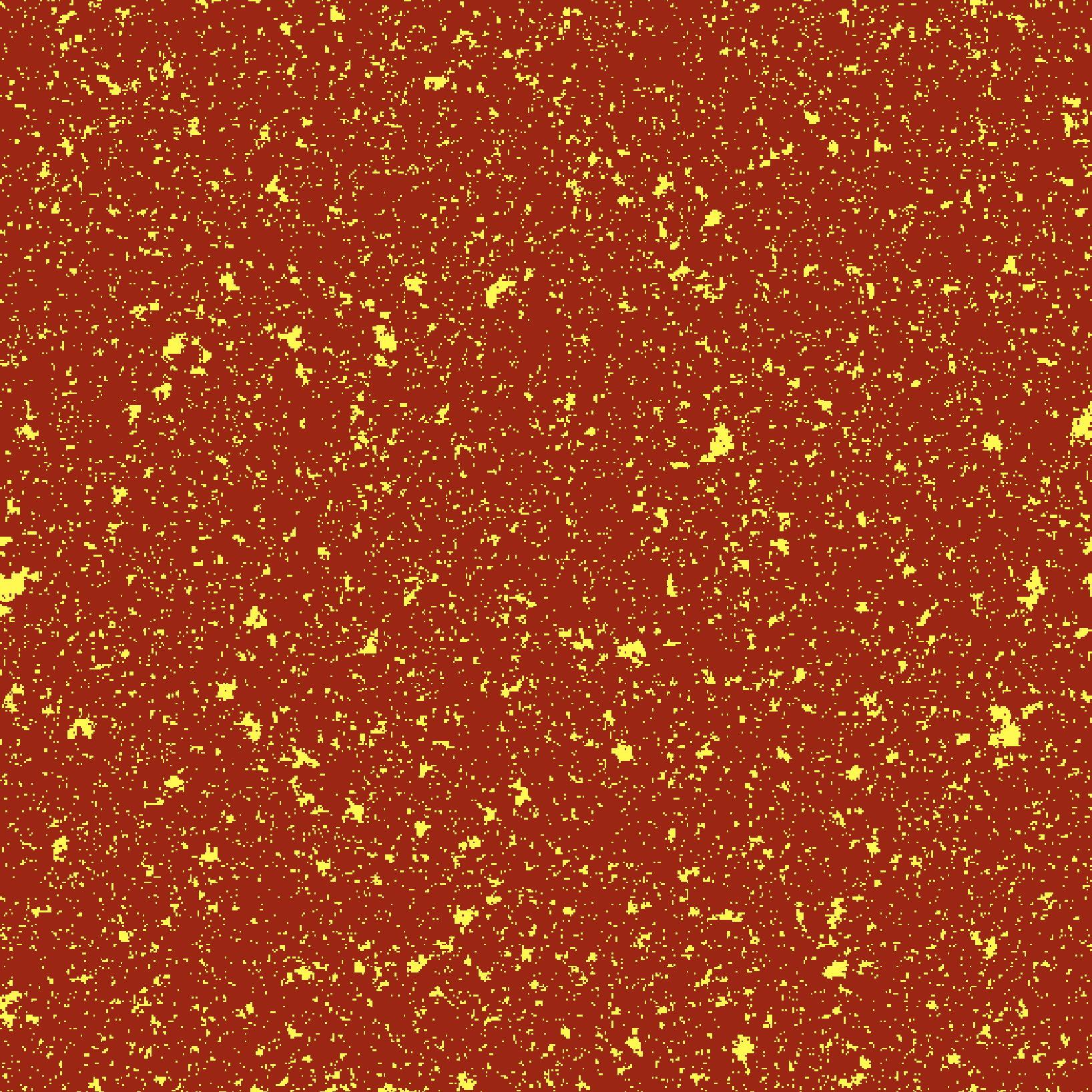
Figure 2: Typical Ising configurations for $\beta<\beta_{c}$ (left) and $\beta>\beta_{c}$ (right).

In many examples of interest (including the case of the Ising model, but not the case of percolation), the measure $\mu_{\beta}=\lim_{N\to\infty}\mu_{\beta,N}$ is well-defined (i.e. independent of the choice of boundary condition) for $\beta<\beta_{c}$ while one can obtain several distinct limits in the case $\beta>\beta_{c}$. Figure 2 shows typical samples drawn from $\mu_{\beta}$ for the Ising model with $\bar{\sigma}\equiv 1$. In the case $\beta>\beta_{c}$, the resulting sample clearly “remembers” the bias introduced by $\bar{\sigma}$ in the sense that a typical configuration consists of a “sea” of spins taking the dominant value $+1$ (brown) with small “islands” of spins taking the value $-1$ (yellow). Had we set $\bar{\sigma}\equiv-1$, we would have obtained a sample with the opposite behaviour, which illustrates the non-uniqueness of the infinite-volume measure $\mu_{\beta}$ in this case. In the case $\beta<\beta_{c}$ on the other hand, each one of the two possible spin values is about equally represented and the measure is symmetric under the substitution $1\leftrightarrow-1$, which illustrates the uniqueness of $\mu_{\beta}$. It is in fact a theorem in the case of the Ising model that for $\beta>\beta_{c}$ there exist exactly two translation invariant infinite volume measures $\mu_{\beta}^{\pm}$ corresponding to boundary conditions $\bar{\sigma}\equiv\pm 1$ and that every accumulation point of $\mu_{\beta,N}$ for any sufficiently homogeneous boundary condition as $N\to\infty$ is a convex combination of $\mu_{\beta}^{+}$ and $\mu_{\beta}^{-}$.

This raises the question of the uniqueness of $\mu_{\beta}$ at $\beta=\beta_{c}$. If it is, then we say that the phase transition is continuous, otherwise it is said to be discontinuous. The reason for this terminology is that continuity in this sense turns out to be equivalent to the continuity of the maps $\beta\mapsto\mu_{\beta}^{\pm}$ at $\beta=\beta_{c}$. It has been known for quite some time [ContTwo, ContHigh] that the phase transition for the Ising model is continuous in dimensions $d=1,2$ as well as $d\geq 4$. The reason why dimensions $1$ and $2$ are typically much better understood is that the Ising model is “solvable” in these dimensions in the sense that explicit expressions can be derived for the expectation of a large number of observables under $\mu_{\beta,N}$ (this solution is straightforward in $d=1$ [Ising] where no phase transition is present, but it was a major breakthrough when Onsager obtained his exact solution for $d=2$ [Onsager]). Dimension $d=4$ on the other hand is the “upper critical dimension” beyond which the model is expected to be “trivial” (i.e. described by Gaussian random variables in the scaling limit) which allows to use a number of powerful techniques, including for example the lace expansion [Lace, LaceIsing].

This leaves the case $d=3$ which is of course the physically most interesting one since the Ising model is a toy model of ferromagnetism and its dimensions represent the usual spatial dimensions. Heuristic considerations suggest that the phase transition is also continuous there, and this is consistent with physical experiments, assuming that the Ising model belongs to the same universality class as that of a genuine physical magnet. In the article [ContIsing], Duminil-Copin et al. gave the first rigorous proof that this is indeed the case. The proof relies on the introduction of the quantity M(β) = inf_B ⊂Z^3 1|B|2 ∑_x,y ∈B ∫σ_xσ_y μ^0_β(dσ) , where $\mu_{\beta}^{0}$ denotes the infinite volume limit obtained from using “free” conditions, as well as three main steps. First, they rely on results of [Infrared, Reflect] to argue that the Fourier transform of $x\mapsto\int\sigma_{0}\sigma_{x}\,\mu_{\beta}^{0}(d\sigma)$ belongs to $L^{1}$ at $\beta=\beta_{c}$, which implies that $M(\beta_{c})=0$. Then, and this is the main step, they show that having $M(\beta)=0$ implies that a certain percolation model with long-range correlations constructed from the Ising model admits no infinite clusters. Finally, they use a variant of the “switching lemma” [Switching] to show that the quantity $\int\sigma_{0}\sigma_{x}\,\mu_{\beta}^{+}(d\sigma)-\int\sigma_{0}\sigma_{x}\,\mu_{\beta}^{0}(d\sigma)$ is dominated by an explicit function times the probability of the origin belonging to an infinite cluster in the above mentioned model and therefore has to vanish at $\beta=\beta_{c}$. Once this is known, it is not too difficult to show that the spontaneous magnetisation of the Ising model at criticality must vanish (namely one has $\int\sigma_{0}\,\mu_{\beta_{c}}^{+}(d\sigma)=0$), which in turn yields the desired uniqueness statement.

To illustrate the fact that continuity of the phase transition, whatever the dimension, is a rather non-trivial property that isn’t necessarily expected in general, a good example is that of the Potts model [Potts]. This is defined similarly to the Ising model, but this time the local state space $S$ is given by $S=\{1,\ldots,q\}$ for some $q\geq 2$ endowed again with the normalised counting measure as its reference measure. As in the Ising model, one sets $H_{A}=0$ unless $A=\{u,v\}$ with $u,v\in\mathbf{Z}^{d}$ such that $|u-v|=1$, in which case one sets $H_{A}(\sigma)=\mathbf{1}_{\sigma_{u}=\sigma_{v}}$. For $q=2$ this is equivalent to the Ising model since their energy functionals only differ by a constant. Let us also remark that there is an essentially equivalent model called the random cluster model (or sometimes the FK model after Fortuin and Kasteleyn who introduced it in [FK]) in which one directly considers partitions of $\mathbf{Z}^{d}$ into connected “clusters” (which one should think of as the edge-connected components of the sets $\{u\,:\,\sigma_{u}=i\}$ for $i\in S$ and a given configuration $\sigma$ of the Potts model) and which makes sense also for non-integer values of $q\geq 1$. (In the case $q=1$ the FK model actually reduces to regular Bernoulli percolation.) See (LABEL:e:defFK) below for a more precise definition of this model.

It was conjectured by Baxter in the 70’s [Baxter1, Baxter2] that the Potts model on $\mathbf{Z}^{2}$ exhibits a continuous phase transition if and only if $q\leq 4$. The pair of articles [PottsDisc, PottsCont] by Duminil-Copin et al. provides proofs of both directions of this conjecture. For the sake of brevity we will not comment on the proofs in any detail, but we note that the proof of continuity of the phase transition for $q\leq 4$ is almost completely disjoint from that in the case of the $3d$ Ising model. A milestone is again to show that the model at criticality with boundary condition set to one fixed element of $S$ admits no infinite cluster. However both the proof of this fact (exploiting a form of discrete holomorphicity of certain cleverly chosen observables) and the proof of its equivalence with the uniqueness of the infinite-volume measure at criticality (actually they show equivalence of a list of $5$ quite distinct properties which are of independent interest for the study of the critical Potts model) are completely different.

Regarding the proof of discontinuity when $q>4$, the main tool is a close relation, first discovered by Temperley–Lieb [TL] in a restricted context and then by Baxter et al. [Baxter_1976] in more generality, between the FK model on $\mathbf{Z}^{2}$ and the so-called six-vertex model. Configurations of the latter can be visualised as jigsaws where one assigns to each vertex of $\mathbf{Z}^{2}$ (or a subset thereof) one of the six (oriented) tiles

[lightgray]1-1-11   [lightgray]-111-1   [lightgray]11-1-1   [lightgray]-1-111   [violet]1-11-1   [violet]-11-11

and one enforces the admissibility constraint that the tiles fit together seamlessly. One further postulates that the probability of seeing a given admissible configuration is proportional to $c^{\#p}$, where $\#p$ denotes the number of purple tiles in the configuration and $c$ is some fixed constant. The relation between the six-vertex model and the critical FK model holds for the specific choice $c=\sqrt{2+\sqrt{q}}$. The advantage gained from this relation is that the six-vertex model is “solvable” in a certain sense using the transfer matrix formalism. This doesn’t get one out of the woods since the transfer matrices $V_{N}$ involved are very large: they act on a vector space of dimension $2^{N}$, but are block diagonal with each block $V_{N}^{[n]}$ acting on a subspace of dimension $\binom{n}{N}$. Each of these blocks is irreducible with positive entries and therefore admits a Perron–Frobenius vector. The main technical result of [PottsDisc] is a very sharp asymptotic for the Perron–Frobenius eigenvalues of $V_{N}^{[N/2-r]}$ for fixed $r$ as $N\to\infty$. Interestingly, the authors are able to prove that the ratios between these values converge to finite (and explicit, at least as explicit convergent series) limits as $N\to\infty$ and that the values themselves diverge exponentially in $N$ with known exponent, but the common lower-order behaviour of that divergence is not known. This asymptotic is however sufficient to obtain good control over the partition function of the six vertex model and to exploit it to compute an explicit expression for the inverse correlation length of the critical Potts model with free boundary conditions when $q>4$. The finiteness of that expression finally allows to deduce the discontinuity of the phase transition.

To conclude this section, I would like to mention the beautiful article [Sharp] which, although not quite dealing with the question of continuity of the phase transition, does have a related flavour. The question there is that of the “sharpness” of the phase transition which in this particular case is couched as the question whether it is really true that the measure $\mu_{\beta}$ has exponentially decaying correlations (in the sense that the covariance between $f(\sigma_{0})$ and $f(\sigma_{x})$ decays exponentially fast as $|x|\to\infty$ for any “nice enough” function $f\colon S\to\mathbf{R}$) for every $\beta<\beta_{c}$ and not just for small enough values where a perturbation argument around $\beta=0$ (where $f(\sigma_{0})$ and $f(\sigma_{x})$ are independent under $\mu_{0}$ as soon as $x\neq 0$) may apply. One difficulty with this type of statements is that one will in general not know any closed-form expression for $\beta_{c}$: in the case of the FK model on the square lattice such an expression can be derived by a duality argument [MR2948685], but it is not known for more general situations. The main result of [Sharp] is that the phase transition of the FK model on any vertex-transitive infinite graph is sharp.

The main tool in their proof is a novel and far-reaching generalisation of the OSSS inequality [OSSS]. The context here is that of increasing random variables $f\colon\{0,1\}^{E}\to[0,1]$ (for a finite set $E$ and for the natural coordinate-wise partial order on $\{0,1\}^{E}$) where $\{0,1\}^{E}$ is furthermore equipped with a probability measure $\mathbf{P}$ that is itself monotonic in the sense that for every $F\subset E$ and every $e\in E\setminus F$, the conditional probabilities $\mathbf{P}(w_{e}=1\,|\,\mathcal{F}_{F})$ are increasing functions. (Here $\mathcal{F}_{F}$ denotes the $\sigma$-algebra generated by the evaluations $w\mapsto w_{e}$ for $e\in F$.) One then considers any algorithm that reveals one by one the values of an input $w\in\{0,1\}^{E}$ in such a way that the coordinate to be revealed next depends in a deterministic way on the information gleaned from the revealement up to that point. (In particular, the first coordinate to be revealed is always the same since no information has been obtained yet at that point.) The algorithm stops once the revealed values are sufficient to determine the value of $f(w)$, thus yielding a random set $\hat{E}\subset E$ of revealed values. The result of [Sharp] is then that one has the inequality [e:CorInequ] Var(f) ≤∑_e ∈E P(e ∈^E)  Cov(f,w_e) , which looks formally the same as the result of [OSSS], but the assumption there was that the measure $\mathbf{P}$ is simply the uniform measure. Since the latter is clearly monotonic (it is such that $\mathbf{P}(w_{e}=1\,|\,\mathcal{F}_{F})$ is constant), the results of [OSSS] follow as a special case.

Using this result, [Sharp] then obtain the following dichotomy which yields the desired sharpness statement.

Theorem 2.1.

Let $G$ be any transitive graph and let $\mathbf{P}_{\beta,n}$ be the FK measure on the ball $\Lambda_{n}$ of radius $n$ in $G$. Then, there exists $\beta_{c}\in\mathbf{R}$ such that, for every $\beta<\beta_{c}$ there exists $c_{\beta}>0$ such that $\mathbf{P}_{\beta,n}(0\leftrightarrow\partial\Lambda_{n})\lesssim e^{-c_{\beta}n}$, uniformly in $n$. For $\beta>\beta_{c}$ on the other hand, there exists $c>0$ such that $\mathbf{P}_{\beta,n}(0\leftrightarrow\partial\Lambda_{n})\geq c\min\{1,\beta-\beta_{c}\}$.

Once (LABEL:e:CorInequ) is known, the proof is surprisingly simple and relies on two ingredients. First, one can show that the measures $\mathbf{P}_{\beta,n}$ and the function $\mathbf{1}_{0\leftrightarrow\partial\Lambda_{n}}$ satisfy the assumptions of (LABEL:e:CorInequ). Setting $\theta_{n}(\beta)=\mathbf{P}_{\beta,n}(0\leftrightarrow\partial\Lambda_{n})$, a clever choice of search algorithm for the (potential) cluster connecting the origin $0$ to $\partial\Lambda_{n}$ then allows to show that one has the bound [e:ineq] θ_n’(β) ≳∑_e ∈E Cov_β(1_0 ↔∂Λ_n ,w_e) ≥n 8Σn(β)θ_n(β) (1-θ_n(β)) . where $\Sigma_{n}=\sum_{k=0}^{n-1}\theta_{n}$. The fact that the first inequality holds is known and can be checked in an elementary way. The second fact is that any sequence of functions $\beta\mapsto\theta_{n}(\beta)$ satisfying a differential inequality of the form (LABEL:e:ineq) necessarily satisfies a dichotomy of the type appearing in the statement of Theorem 2.1. Since we are not interested in the regime where $\theta_{n}$ is large, we can rewrite (LABEL:e:ineq) as $\theta_{n}^{\prime}\geq{cn\over\Sigma_{n}}\theta_{n}$. The fact that the $\theta_{n}$ then should satisfy such a dichotomy is quite clear: if $\beta$ is such that they converge to a non-vanishing limit $\theta$, then $\Sigma_{n}/n\sim\theta$ and one must have $\theta^{\prime}\geq c$. If on the other hand they converge to $0$ on a whole interval $[a,b]$, then that convergence must take place sufficiently fast so that $\Sigma_{n}/n\gg\theta_{n}$ (since otherwise the previous argument applies). Since $\Sigma_{n}/n\sim\theta_{n}$ for $\theta_{n}\sim n^{-\alpha}$ as soon as $\alpha<1$, it is then plausible that for any $c<b$ one has $\theta_{n}\ll n^{-1/2}$ (say), implying $\theta_{n}^{\prime}\gtrsim\sqrt{n}\theta_{n}$ and therefore $\theta_{n}\lesssim e^{-\sqrt{n}(c-\beta)}$ for $\beta<c$. This shows that $\Sigma_{n}$ is bounded for $\beta<c$, leading to $\theta_{n}^{\prime}\gtrsim n\theta_{n}$ and therefore an exponentially (in $n$) small bound as claimed.

3 Triviality of m1[]$\Phi^{4}_{4}$

It has been known since the groundbreaking work of Osterwalder and Schrader [OS, OS2] that, at least in some cases, the construction of a (bosonic) quantum field theory satisfying the Wightman axioms is equivalent to the construction of a probability measure on the space of distributions satisfying a number of natural properties. One of the pinnacles of that line of enquiry was the construction in the seventies of the $\Phi_{2}^{4}$ and $\Phi_{3}^{4}$ measures [Nelson1, Nelson2, Simon, MR0231601, MR0359612, MR0408581, MR0384003, MR0416337], which corresponds to the simplest case of an interacting theory in two or three space-time dimensions with one type of boson.

At a heuristic level, the $\Phi_{d}^{4}$ measure is the measure $\mu^{(d)}$ on the space of Schwartz distributions $\mathcal{S}^{\prime}(\mathbf{R}^{d})$ (or on the $d$-dimensional torus) given by μ^(d)(dΦ) = Z^-1 exp(- 12 ∫(|∇Φ(x)|^2 - C Φ^2(x) + Φ^4(x)) dx)  dΦ , where “$d\Phi$” denotes the infinite-dimensional Lebesgue measure on $\mathcal{S}^{\prime}(\mathbf{R}^{d})$. This expression is of course problematic at many levels: infinite-dimensional Lebesgue measure does not exist, distributions cannot be squared, etc. If it were only for the term $|\nabla\Phi|^{2}$, one could reasonably interpret this expression as the Gaussian measure $\mu_{0}$ with covariance operator given by the Green’s function of the Laplacian, which is a well-defined probability measure (modulo technicalities arising from the constant mode which can easily be fixed). The measure $\mu_{0}$ is called the Gaussian Free Field (GFF) since it corresponds to a quantum field theory in which particles are free, i.e. do not interact with each other at all.

This suggests that a more refined interpretation of the $\Phi^{4}_{d}$ measure could be given by [e:defNaive] μ^(d)(dΦ) = Z^-1 exp(- 12 ∫Φ^4(x) dx ) μ_0(dΦ) . This is still ill-defined since the GFF is supported on distributions rather than functions for any dimension $d\geq 2$. However, setting $\Phi_{\varepsilon}=\rho_{\varepsilon}\star\Phi$, the Wick power [e:Wick] :Φ^4: = lim_ε→0 (Φ_ε^4 - 3 Φ_ε^2 EΦ_ε