A new formulation of strong-field magnetohydrodynamics for neutron stars

Abstract

We present a formulation of magnetohydrodynamics which can be used to describe the evolution of strong magnetic fields in neutron star interiors. Our approach is based on viewing magnetohydrodynamics as a theory with a one-form global symmetry and developing an effective field theory for the hydrodynamic modes associated with this symmetry. In the regime where the local velocity and temperature variations can be neglected, we derive the most general constitutive relation consistent with symmetry constraints for the electric field in the presence of a strong magnetic field. This constitutive relation not only reproduces the phenomena of Ohmic decay, ambipolar diffusion, and Hall drift derived in a phenomenological model by Goldreich and Reisenegger, but also reveals new terms in the evolution of the magnetic field which cannot easily be seen from such microscopic models. This formulation gives predictions for novel diffusion behaviors of small perturbations around a constant background magnetic field, and for the two-point correlation functions among various components of the electric and magnetic fields.

Introduction.— Hydrodynamics provides a universal description of an interacting many-body system in the large distance and long time limit by capturing the effective dynamics of conserved quantities. For an electrically conducting fluid with a magnetic field, it is necessary to incorporate electromagnetism in describing the motion of the fluid, leading to magnetohydrodynamics (MHD). MHD plays an important role in many disciplines including plasma physics, astrophysics, and cosmology. In this paper, we provide a new formulation of MHD at strong magnetic fields for neutron stars, which exhibit some of the strongest (up to $10^{11}$ Tesla) and most dramatically variable magnetic fields in the universe (see Refs. Lattimer and Prakash (2004); Kaspi and Beloborodov (2017); Harding and Lai (2006)). We also discuss some immediate implications of the new theory for magnetic diffusion.

The dynamical variables of MHD for a neutral fluid include the local velocity $\mathbf{v}(x)$, local temperature $T(x)$, and magnetic field $\mathbf{B}(x)$. Here bold-face letters denote spatial vectors. The equations of motion consist of the conservation of the energy-momentum tensor $\partial_{\mu}T^{\mu\nu}=0$ , and two of the Maxwell equations,

$$\nabla\cdot{\bf B}=0,\quad\partial_{t}{\bf B}=-\nabla\times{\bf E}.$$ (1)

The components of $T^{\mu\nu}$ and ${\bf E}$ are expressed in terms of the hydrodynamical variables via constitutive relations. In the standard formulation of MHD, such relations are written on phenomenological grounds and become ambiguous in the presence of a strong magnetic field.

In applications to a neutron star, a frequently-used approximation to illustrate some of the main physical effects is to take $\mathbf{v}(x)=0$ and $T(x)={\rm const}$. In Goldreich and Reisenegger (1992), a phenomenological model for neutron stars was used to derive an expression for E in terms of B as well as fast-evolving microscopic variables such as the densities of electrons and protons. The results of Goldreich and Reisenegger (1992) have been used to formulate MHD equations in a variety of contexts, both in neutron star physics Gourgouliatos and Cumming (2014); Castillo et al. (2017); Bransgrove et al. (2018); Lattimer and Prakash (2004); Kaspi and Beloborodov (2017); Harding and Lai (2006); Thompson and Duncan (1993, 1995); Urpin and Shalybkov (1999); Cumming et al. (2004); Cho and Lazarian (2004); Reisenegger et al. (2005); Mereghetti et al. (2015); Passamonti et al. (2017); Pons and Viganò (2019) and in astrophysics more generally Brandenburg and Zweibel (1994); Brandenburg and Subramanian (2005); Balbus (2009). Despite these successes, the inadequate knowledge of particle interactions inside neutron stars makes it difficult to assess the accuracy of such formulations or to improve upon them systematically using phenomenological approaches.

In this paper, we provide a new formulation of strong-field MHD based on effective field theory, which makes it possible to derive the most general constitutive relations consistent with the symmetries of the system, regardless of the details of microscopic interactions (such as whether weak interactions are included or not). For illustration of the formalism, we will use the static neutron approximation, and neglect possible neutron superfluidity and proton superconductivity Glampedakis et al. (2010); Dommes and Gusakov (2021). Our theory is valid in the regime where all other physical quantities relax much faster than $\mathbf{B}$. Our main result is a constitutive relation for ${\bf E}$ in terms of ${\bf B}$ given in (7), which together with (1) gives a closed equation for the evolution of ${\bf B}$. In this paper, we outline the derivation of this result and its consequences, leaving a detailed exposition of the effective field theory to Grozdanov et al. .

Our formulation combines two significant recent developments. The first ingredient is a new formulation of hydrodynamics as the low energy effective field theory (EFT) of a general many-body system Crossley et al. (2017); Glorioso et al. (2017) (see Glorioso and Liu (2018) for a review and also Grozdanov and Polonyi (2015); Haehl et al. (2016); Jensen et al. (2018)). In addition to providing a systematic framework for treating hydrodynamical fluctuations, the new EFT approach also has a number of advantages at the level of equations of motion compared with the traditional approach. It provides a systematic derivation of the constitutive relations without the need of imposing any phenomenological constraints by hand, and introduces an alternative set of dynamical variables that are often more convenient than traditional ones. The second ingredient is the important observation of Grozdanov et al. (2017) that MHD can be formulated as an effective field theory for a system with a higher-form global symmetry Gaiotto et al. (2015). See Hernandez and Kovtun (2017); Grozdanov and Poovuttikul (2019); Glorioso and Son (2018); Armas and Jain (2020); Gralla and Iqbal (2019); Benenowski and Poovuttikul (2019); Landry (2021); Armas and Camilloni (2022) for various developments. This makes it possible to formulate MHD based on symmetries alone.

MHD for neutron stars.—The basic idea behind the formulation of MHD in Grozdanov et al. (2017) is that the MHD equations (1) can be written as the conservation equations for a two-form current $J^{\mu\nu}=-J^{\nu\mu}$:

$$\partial_{\mu}J^{\mu\nu}=0,\quad J^{0i}=B^{i},\quad J^{ij}=-\epsilon^{ijk}E^{k},$$ (2)

i.e., $J^{\mu\nu}=\tilde{F}^{\mu\nu}=\frac{1}{2}\epsilon^{\mu\nu\rho\sigma}F_{\rho\sigma}$. Accordingly, equations (1) can be interpreted as resulting from an underlying one-form symmetry. This realization is not simply a renaming of equations (1), but provides a powerful symmetry principle for formulating MHD. In particular, the choice of dynamical variables and the structure of the constitutive relation are dictated by this symmetry principle.

An effective action for a dissipative hydrodynamic system can be formulated in terms of the closed-time-path (CTP) or Schwinger-Keldysh formalism (for a review of these methods, see Glorioso and Liu (2018)). A key ingredient of the formulation of Crossley et al. (2017); Glorioso et al. (2017) is the fact that the dynamical hydrodynamic variables are the Stueckelberg fields associated with the global symmetries responsible for the conservation laws. For the one-form symmetry relevant for MHD, this is a vector field $A_{\mu}$, which is a collective effective field describing the long-distance and long-time behavior (not the microscopic electromagnetic potential for $\bf E$ and $\bf B$ fields of the system).

The hydrodynamic effective action $S_{\rm EFT}$ for MHD is then the most general action written in terms of the combination $G_{\mu\nu}\equiv b_{\mu\nu}+\partial_{\mu}A_{\nu}-\partial_{\nu}A_{\mu}$ that is invariant under various symmetries. Here, for later convenience, we have also turned on an external source $b_{\mu\nu}$ for the two-form current $J^{\mu\nu}$. The symmetries to be imposed can be separated into those universal for all hydrodynamic systems Crossley et al. (2017); Glorioso et al. (2017) and those specific to the system under study. A neutron star can be regarded as a neutral plasma consisting of electrons, protons, and neutrons. In this system, the energy is high enough that electrons can be treated as relativistic, but not high enough for the existence of positrons. Thus, the charge conjugation $\mathcal{C}$ is badly broken. Weak interactions also break parity $\mathcal{P}$. See Appendix A for the explicit form of the action. Here, we give the final form of the constitutive relations for $J^{\mu\nu}$ at the lowest dissipative order:

$$J^{0i} = a\,G_{0i}+m\,\delta_{ij}{\epsilon}_{kln}G_{0n}H_{jkl},$$ (3)

$$J^{ij} = -2\beta_{0}(d\,\delta_{ik}\delta_{jl}+\tilde{d}\,\epsilon_{ijm}{\epsilon}_{kln}G_{0m}G_{0n})\partial_{0}G_{kl}$$ (4)

$$- m\,\epsilon_{lij}\partial_{l}G_{0k}^{2}+2p\,\delta_{k[i}\epsilon_{j]ln}G_{0n}\partial_{0}G_{kl},$$ (5)

where $H_{\mu\nu\lambda}=\partial_{\mu}b_{\nu\lambda}+\partial_{\lambda}b_{\mu\nu}+\partial_{\nu}b_{\lambda\mu}$ and $[ij]\equiv{1\over 2}(ij-ji)$. All coefficients $a,d,\tilde{d},m,p$ should be understood as functions of $G_{0i}^{2}$, and they satisfy the constraints

$$a\geq 0,\quad d\geq 0,\quad d+2\tilde{d}\,G_{r0i}^{2}\geq 0.$$ (6)

We can write (3)–(4) in a more conventional form by solving for $G_{0i}$ in terms of $J^{0i}=B^{i}$. Then on setting $b_{\mu\nu}=0$ , (4) can be written as the constitutive relation for the electric field:

$${\bf E} =\eta\,{\bf j}+c_{a}\,({\bf j}\times{\bf B})\times{\bf B}+c_{H}\,{\bf j}\times{\bf B}$$ (7)

$$-c_{H}(\nabla\ln a({\bf B}^{2})\times{\bf B})\times{\bf B}-c_{\eta}\nabla\ln a({\bf B}^{2})\times{\bf B}+\nabla f,$$

where ${\bf j}\equiv\nabla\times{\bf B}$, and we have introduced a function $f$ of ${\bf B}^{2}$ such that $m=f^{\prime}$. The coefficients are

$$\eta=c_{\eta}+c_{a}\mathbf{B}^{2},~{}c_{\eta}=\frac{2\beta_{0}d}{a},~{}c_{a}=\frac{4\beta_{0}\tilde{d}}{a^{3}},~{}c_{H}=-\frac{2p}{a^{2}},$$ (8)

where $\beta_{0}=1/T$ is the constant inverse temperature. Now all coefficients should be understood as functions of $\mathbf{B}^{2}$. We will see below that $a(\mathbf{B}^{2})$ can be interpreted as a susceptibility in the linear response theory around a constant background magnetic field ${\bf B}$, and must therefore be non-negative. Note that $\nabla\ln a({\bf B}^{2})=\frac{a^{\prime}}{a}\nabla{\bf B}^{2}$, and, hence, is proportional to the gradient of the magnetic energy density. Coefficients $c_{\eta}$ and $\eta$ will be interpreted as magnetic “diffusivities.” From (6), we must have

$$\eta\geq 0,\quad c_{\eta}\geq 0.$$ (9)

Note that (7) can also be written in terms of the three independent coefficients $c_{\eta}$, $c_{a}$ and $c_{H}$ as

$${\bf E}=c_{\eta}\,{\bf j}_{B}+c_{a}\,({\bf B}\cdot{\bf j})\,{\bf B}+c_{H}\,{\bf j}_{B}\times{\bf B}+\nabla f,$$ (10)

$${\bf j}_{B}={\bf j}-\nabla\ln a({\bf B}^{2})\times{\bf B}.$$ (11)

The first line of (7) includes each of the explicitly ${\bf B}$-dependent terms derived in equation (13) of Goldreich and Reisenegger (1992), that lead to behaviors in the magnetic field evolution known as Ohmic decay, ambipolar diffusion, and Hall drift respectively. The terms in the second line of (7) are not explicitly present in Goldreich and Reisenegger (1992). Moreover, unlike in Goldreich and Reisenegger (1992), the coefficients $\eta$, $c_{a}$, and $c_{H}$ are all functions of ${\bf B}$ in (7). Note also that the value of $c_{a}$, which is negative in Goldreich and Reisenegger (1992), can in principle have either sign here. If negative, its absolute value is bounded by $|c_{a}|\mathbf{B}^{2}<c_{\eta}$ due to (9).

In comparing the two formulations, it is important to note that equation (13) of Goldreich and Reisenegger (1992) includes additional terms dependent on the density $n_{c}$ of the electrons or protons, and that the analogs of the coefficients $\eta$, $c_{a}$, and $c_{H}$ appearing there also depend on $n_{c}$. However, as discussed in Castillo et al. (2017), $n_{c}$ evolves on a much faster time scale than ${\bf B}$, and can be seen as fully determined by $\bf B$ on the time scales relevant for MHD. We therefore expect one source of the $\bf B$-dependence of the coefficients in our general constitutive relation (7) to be the $\bf B$-dependence of $n_{c}$. Similarly, it may be possible to see the terms in the second line of (7) by appropriately “integrating out” $n_{c}$ from the model of Goldreich and Reisenegger (1992); Castillo et al. (2017) .

Here we see the major advantages of our formulation. The constitutive relation of $\mathbf{E}$ in terms of $\mathbf{B}$ is rather complicated, and there appears to be no general principle to write it down directly. But in terms of the new dynamical variables $A_{\mu}$ (or equivalently $G_{0i}$), the fields $\mathbf{E}$ and $\mathbf{B}$ are given in a parametric form in (3)–(4), which can be written down systematically and straightforwardly based on symmetries and derivative expansions. We believe the parametric form (3)–(4) is likely also more convenient for nonlinear numerical simulations.

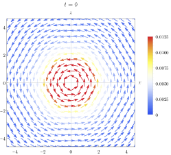
Figure 1: Evolution of the initial magnetic field configuration ${\bf B}(0,\mathbf{x})=\frac{\sqrt{\pi}}{(2\pi)^{2}}\frac{r}{w^{3}}e^{-\frac{r^{2}}{2w^{2}}}\left[I_{0}\left(\frac{r^{2}}{2w^{2}}\right)-I_{1}\left(\frac{r^{2}}{2w^{2}}\right)\right]{\hat{\phi}}$, where $r,\phi$ are the polar coordinates in the $x-z$ plane, and $I_{n}(r)$ is the modified Bessel function of the first kind. We take $w=1$ and $\sigma_{1}^{\perp}=1$. The left figure shows the initial condition. The middle figure shows the configuration at $t=2$ with $\chi_{\parallel}=\chi_{\perp}=1$, while the right figure shows the configuration at $t=2$ with $\chi_{\parallel}=1$ and $\chi_{\perp}=8$. The color bars indicate the magnitude of ${\bf B}$.

Magnetic diffusion with a strong background magnetic field.—To develop intuition for the physics encoded in (3)–(4) (or equivalently, (7)), we consider the behavior of small perturbations around a constant $\bf B$ along the $z$ direction with magnitude $B_{0}$. Such a constant magnetic field configuration can be conveniently thought of as being due to a constant background ‘chemical potential’ $b_{0z}=\mu$ with $B_{0}=a(B_{0}^{2})\mu$. For small perturbations around such a configuration, we can write

$$\!\!G_{\mu\nu}=\mu\delta_{0[\mu}\delta_{\nu]z}+f_{\mu\nu},\;\,f_{\mu\nu}=b_{\mu\nu}+\partial_{\mu}A_{\nu}-\partial_{\nu}A_{\mu},$$ (12)

where we have also introduced an infinitesimal external source $b_{\mu\nu}$ and we will work to linear order in both $b_{\mu\nu}$ and $f_{\mu\nu}$. Expanding (3)–(4) in small $f_{\mu\nu}$ we then find

$$J^{0z} =B_{0}+\chi_{\parallel}f_{0z}+2m\mu H_{xyz},\quad J^{0a}=\chi_{\perp}f_{0a},$$ (13)

$$J^{za} =-(\sigma_{1}^{\perp}\delta_{ab}+\sigma_{2}^{\perp}\epsilon_{ab})(H_{0zb}+\partial_{z}f_{0b})$$ (14)

$$+\left[\sigma_{1}^{\perp}\delta_{ab}+(\sigma_{2}^{\perp}-2m\mu)\epsilon_{ab}\right]\partial_{b}f_{0z},$$ (15)

$$J^{xy} =-\sigma^{\parallel}(H_{0xy}+K_{xy})-2m\mu\partial_{z}f_{0z},$$ (16)

where subscripts $a,b$ index $x,y$ directions, and

$$\chi_{\parallel}=a+\tilde{a}B_{0}^{2},\quad\chi_{\perp}=a,\quad\tilde{a}=2a^{\prime}(B_{0}^{2}),$$ (17)

$$\sigma_{1}^{\perp}=c_{\eta}\chi_{\perp}\quad\sigma_{2}^{\perp}={B_{0}\over 2}c_{H}\chi_{\perp},\quad\sigma^{\parallel}=\eta\chi_{\perp},$$ (18)

$$\qquad K_{xy}\equiv\partial_{x}f_{0y}-\partial_{y}f_{0x},$$ (19)

with all coefficients evaluated at ${\bf B}^{2}=B_{0}^{2}$. As discussed in Appendix A, systems with charge conjugation symmetry have $p=0$, and hence ${\sigma}_{2}^{\perp}=0$. We stress that $\tilde{a}$ arises from $\mathbf{B}$-dependence of the coefficient $a$, and hence cannot be seen naively from the formulation of Goldreich and Reisenegger (1992), where all coefficients appear to be $\mathbf{B}$-independent.

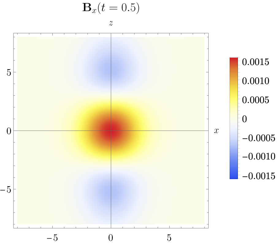
Figure 2: Different components of ${\bf B}$ at $t=0.5$, evolved from the initial configuration ${\bf B}(0,\mathbf{x})=\frac{1}{\pi\sigma^{2}}\,e^{-\frac{x^{2}+z^{2}}{\sigma^{2}}}\hat{y}$. All planes orthogonal to the $y$ direction are identical. The parameter values are $\sigma_{1}^{\perp}=4$, $\sigma^{\parallel}=2$, $\sigma_{2}^{\perp}=-1$, $\chi_{\perp}=1$, and $\chi_{\parallel}=8$.

The functions $\chi_{\perp}$ and $\chi_{\parallel}$ can be interpreted as magnetic susceptibilities, defined by the Kubo formulas

$$\chi_{\parallel}=\lim_{\mathbf{k}\to 0}\lim_{\omega\to 0}G^{R}(B_{z},B_{z}),\quad\chi_{\perp}=\lim_{\mathbf{k}\to 0}\lim_{\omega\to 0}G^{R}(B_{x},B_{x}),$$ (20)

where $G^{R}(B_{z},B_{z})$ denotes the retarded correlation functions of $B_{z}$ and $B_{z}$, and similarly for other components (see Appendix B for details). From thermodynamic stability we should have $\chi_{\perp}\geq 0,\chi_{\parallel}\geq 0$. In the linear response theory derived from Goldreich and Reisenegger (1992), we have $\chi_{{\parallel}}=\chi_{\perp}$ since $\tilde{a}=0$, but more generally, these susceptibilities should be different.

The ${\sigma}$’s can be interpreted as magnetic “viscosities”, defined by the Kubo formulas

$${\sigma}^{\parallel}=\lim_{\omega\to 0}\lim_{\mathbf{k}\to 0}{1\over i\omega}G^{R}(E_{z},E_{z}),$$ (21)

$${\sigma}^{\perp}_{1}=\lim_{\omega\to 0}\lim_{\mathbf{k}\to 0}{1\over i\omega}G^{R}(E_{x},E_{x}),$$ (22)

$${\sigma}^{\perp}_{2}=\lim_{\omega\to 0}\lim_{\mathbf{k}\to 0}{1\over i\omega}G^{R}(E_{x},E_{y}),$$ (23)

where ${\sigma}^{\perp}_{2}$ can be understood as a “Hall” magnetic viscosity. We stress the differences in the order of limits between (20) and (21)–(23). Comparing (9) and (18),

$$\sigma^{{\parallel}}\geq 0,\quad\sigma_{1}^{\perp}\geq 0,$$ (24)

but $\sigma_{2}^{\perp}$ can have either sign. Note that ${\sigma}^{\parallel}-{\sigma}^{\perp}_{1}\propto c_{a}$, and thus the effect of the ambipolar term at this order is to generate anisotropy in the magnetic viscosities.

The equations of motion following from (13)–(16) are a set of coupled diffusion equations, which give the following dispersion relations (see Appendix B for details):

$$\omega=-i{{\sigma}^{\perp}_{1}\over\chi_{\perp}}k_{z}^{2}-\frac{i}{2}\left({{\sigma}^{\parallel}\over\chi_{\perp}}+{{\sigma}^{\perp}_{1}\over\chi_{\parallel}}\right)k_{\perp}^{2}$$ (25)

$$\mp\frac{i}{2}\sqrt{\left({{\sigma}^{\parallel}\over\chi_{\perp}}-{{\sigma}^{\perp}_{1}\over\chi_{\parallel}}\right)^{2}k_{\perp}^{4}-4\left(\frac{{\sigma}^{\perp}_{2}}{\chi_{\perp}}\right)^{2}\left(k_{z}^{2}+\frac{\chi_{\perp}}{\chi_{\parallel}}k_{\perp}^{2}\right)k_{z}^{2}},$$

where $k_{\perp}^{2}=k_{x}^{2}+k_{y}^{2}$. The special case of (25) with $\chi_{{\parallel}}=\chi_{\perp}$ was derived from the formulation of Goldreich and Reisenegger (1992) in Viganò et al. (2019). Note also the special cases

$$k_{\perp}=0: \quad\omega=-{i\over\chi_{\perp}}({\sigma}_{1}^{\perp}\pm i{\sigma}_{2}^{\perp})k_{z}^{2},$$ (26)

$$k_{z}=0: \quad\omega=-i{{\sigma}^{\parallel}\over\chi_{\perp}}k_{\perp}^{2}\;\;\text{or}\;\;\omega=-i{{\sigma}^{\perp}_{1}\over\chi_{\parallel}}k_{\perp}^{2}.$$ (27)

The above dispersion relations lead to interesting patterns in the diffusion of magnetic field lines. First consider ${\sigma}_{2}^{\perp}=0$, in which case (25) becomes

$$\omega=-{i\over\chi_{\perp}}\left({\sigma}^{\perp}_{1}k_{z}^{2}+{\sigma}^{{\parallel}}k_{\perp}^{2}\right)\;\;\text{or}\;\;\omega=-i{\sigma}^{\perp}_{1}\left({k_{z}^{2}\over\chi_{\perp}}+{k_{\perp}^{2}\over\chi_{\parallel}}\right).$$ (28)

Both modes diffuse anisotropically between $z$ and some direction in the $x-y$ plane. When either ${\sigma}^{\perp}_{1}={\sigma}^{{\parallel}}$ (i.e., $c_{a}=0$) or $\chi_{\perp}=\chi_{\parallel}$, one of the modes becomes isotropic. See Fig. 1 for an example of the qualitatively different evolutions with $\chi_{\perp}=\chi_{{\parallel}}$ and $\chi_{\perp}\neq\chi_{{\parallel}}$ .

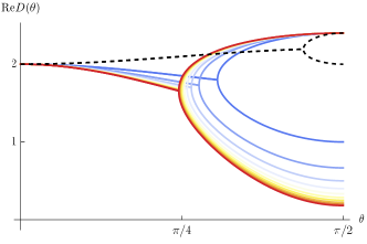
Figure 3: Real and imaginary parts of $D(\theta)=i\omega/k^{2}$ for the following choice of parameters: $\beta_{0}=\mu=p=a=d=1$ and $\tilde{d}=0.1$, where $k_{\perp}=k\sin\theta$ and $k_{z}=k\cos\theta$, for $\theta\in[0,\pi/2]$. The black dashed line represents $\tilde{a}=0$ (corresponding to the theory in Goldreich and Reisenegger (1992)) and the colored lines represent $\tilde{a}={1,2,\ldots,10}$, going from blue to red with other parameters fixed.

A simple example illustrating the consequences of the full dispersion relation (25) is given in Fig. 2, where the initial ${\bf B}$ points in the $y$ direction and is concentrated around the $y$ axis. The $B_{y}$ component diffuses anisotropically, and in addition $B_{x}$ and $B_{z}$ components are also generated and subsequently diffuse. Similar patterns were previously observed in nonlinear simulations of neutron stars in Viganò et al. (2019) and of magnetized filamentary clouds in Burge et al. (2016). We see here that these effects may be understood as simple consequences of the dispersion relations (25). Note that if we had set $\sigma^{\perp}_{2}=0$ for the initial condition in Fig. 2, we would still see anisotropic diffusion of $B_{y}$, but the $B_{x}$ and $B_{z}$ components would remain zero for all times.

Equation (25) has the form $\omega=-iD(\theta)k^{2}$, where $k^{2}=k_{z}^{2}+k_{\perp}^{2}$ and $\theta$ is the angle between the background $\bf B$ and $\mathbf{k}$. In general, for ${\sigma}_{2}^{\perp}\neq 0$, $D(\theta)$ is complex, with its real part being the “diffusion constant” and the imaginary part describing oscillatory propagation. Such propagating behavior was considered in Goldreich and Reisenegger (1992) as a mechanism for the transport of magnetic energy from the inner to the outer crust in neutron stars. $D(\theta)$ at $\theta=0$ and $\theta={\pi\over 2}$ can be read from (26)–(27), while for general $\theta$, it is plotted in Fig. 3. There is a critical value $\theta_{c}$ beyond which $\text{Im}D(\theta)$ for both modes vanishes, and the real parts become different. We also notice that as $\chi_{\parallel}-\chi_{\perp}$ is increased (with other parameters fixed), $\theta_{c}$ decreases.

The effective action formulation allows us to understand the precise way in which the sources $b_{\mu\nu}$ are coupled to the magnetohydrodynamic variables, and hence enables us to obtain the retarded two-point functions among components of $\mathbf{E}$ and $\mathbf{B}$. The full expressions for generic $\mathbf{k}$ are complicated, and are presented in Appendix B. As an example, consider the special case with nonzero $k_{z}$ only, where we find that the nonzero correlation functions among the ${\bf B}$ components are given by

$$G^{R}(B_{x},B_{x}) =\frac{k_{z}^{2}\chi_{\perp}(k_{z}^{2}\xi^{2}-i\sigma_{1}^{\perp}\chi_{\perp}\omega)}{k_{z}^{4}\xi^{2}-2ik_{z}^{2}\sigma_{1}^{\perp}\chi_{\perp}\omega-\chi_{\perp}^{2}\omega^{2}},$$ (29)

$$\qquad G^{R}(B_{x},B_{y}) =\frac{-ik_{z}^{2}\chi_{\perp}\sigma_{2}^{\perp}\chi_{\perp}\omega}{k_{z}^{4}\xi^{2}-2ik_{z}^{2}\sigma_{1}^{\perp}\chi_{\perp}\omega-\chi_{\perp}^{2}\omega^{2}},$$ (30)

where $\xi=\sqrt{{\sigma_{1}^{\perp}}^{2}+{\sigma_{2}^{\perp}}^{2}}$. The mixed nonzero correlation functions among ${\bf E}$ and ${\bf B}$ field components are

$$G^{R}(B_{x},E_{x}) =\frac{\omega}{k_{z}}G^{R}(B_{x},B_{y}),$$ (31)

$$G^{R}(B_{x},E_{y}) =-\frac{\omega}{k_{z}}G^{R}(B_{x},B_{x}),$$ (32)

and among the ${\bf E}$ field components are

$$G^{R}(E_{z},E_{z}) =-\frac{4k_{z}^{2}m^{2}\mu^{2}}{\chi_{{\parallel}}}+i\sigma^{\parallel}\omega,$$ (33)

$$G^{R}(E_{x},E_{x}) =\frac{\omega^{2}}{k_{z}^{2}}G^{R}(B_{x},B_{x}),$$ (34)

$$G^{R}(E_{x},E_{y}) =\frac{\omega^{2}}{k_{z}^{2}}G^{R}(B_{x},B_{y}).$$ (35)

(21)–(23) arise by taking $k_{z}\to 0$ in the above expressions, while the definition of $\chi_{\perp}$ in (20) can be seen by taking $\omega\to 0$ with $k_{z}$ finite. Note that while from (7), the coefficient $m$ plays no role in the equation of motion of the magnetic field at leading order in derivatives, it does appear at leading order in the correlation functions among electric field components, as in (33).

Discussion.—We have developed a new formulation for MHD applicable to neutron stars, in the presence of strong magnetic fields and in the regime where flow velocities and temperature variations can be neglected. This theory leads to the most general constitutive relation for the electric field in terms of the magnetic field for this setup, which in particular reproduces the phenomena of Ohmic decay, ampibolar diffusion, and Hall drift derived in previous formulations such as Goldreich and Reisenegger (1992). Moreover, the constitutive relation includes new terms which systematically take into account all possible contributions that could be obtained from integrating out microscopic degrees of freedom in previous formulations. As a simple application of our formulation, we examined the behavior of small perturbations on top of a strong constant magnetic field, and uncovered novel magnetic diffusion patterns. We also found the two-point correlation functions among electric and magnetic field components.

It will be of great interest to apply our formalism to more realistic problems concerning neutron stars and other astrophysical systems with strong magnetic fields, using full nonlinear evolution based on (7). In particular, it would be interesting to see if the new terms in the second line of (7) lead to qualitatively new phenomena which were not accessible with earlier simulations such as those in Gourgouliatos and Cumming (2014); Castillo et al. (2017); Bransgrove et al. (2018). The MHD formulation here can be generalized to include flow velocities, going beyond the static neutron approximation, as well as temperature variations. It would also be interesting to include the effects of superfluidity or superconductivity, extending the discussion of Glampedakis et al. (2010); Dommes and Gusakov (2021).

Acknowledgements.—We would like to thank Deepto Chakrabarty, Michael Landry, Nick Poovuttikul and in particular Andreas Reisenegger for very helpful discussions. S.G. was supported by the STFC Ernest Rutherford Fellowship ST/T00388X/1 and the research programme P1-0402 of Slovenian Research Agency (ARRS). This work is supported by the Office of High Energy Physics of U.S. Department of Energy under grant Contract Number DE-SC0012567 and DE-SC0020360 (MIT contract # 578218). S.L. acknowledges the support of the Natural Sciences and Engineering Research Council of Canada (NSERC).

Appendix A Appendix A: Details of the effective CTP action for MHD

In this Appendix, we outline the steps leading to (3)–(6). See Grozdanov et al. for technical details, other generalizations, and a more extensive discussion.

The hydrodynamical variables for MHD in the static neutron approximation are given by two vector fields $A_{1\mu},A_{2\mu}$, as on a closed time path all quantities come in two copies. The one-form symmetry implies that the action $S_{\rm EFT}$ can only depend on the dynamical variables $A_{s\mu}$ ($s$ labels the copies) through the combinations

$$G_{s\mu\nu}\equiv b_{s\mu\nu}+\partial_{\mu}A_{s\nu}-\partial_{\nu}A_{s\mu},\quad s=1,2,$$ (36)

where $b_{\mu\nu}$ denotes the external source for the two-form current $J^{\mu\nu}$. By definition, $G_{s\mu\nu}$ and thus $S_{\rm EFT}$ are invariant under the transformation $A_{s\mu}\rightarrow A_{s\mu}+\partial_{\mu}\alpha_{s}$, for arbitrary functions $\alpha_{s}$. We can use the freedom to set $A_{s0}=0$. $S_{\rm EFT}[G_{1\mu\nu},G_{2\mu\nu}]$ is then the most general action invariant under a number of symmetries.

To describe the symmetries to be imposed, it is convenient to introduce the Keldysh basis of symmetric (“$r$”) and antisymmetric (“$a$”) combinations of all fields: $\varphi_{r}\equiv(\varphi_{1}+\varphi_{2})/2$ and $\varphi_{a}\equiv\varphi_{1}-\varphi_{2}$. The symmetries that the MHD action $S_{\rm EFT}$ should satisfy include Crossley et al. (2017); Glorioso et al. (2017):

$$\text{Diagonal shift}:\quad A_{ri}(t,\mathbf{x})\rightarrow A_{ri}(t,\mathbf{x})+\lambda_{i}(\mathbf{x}),$$ (37)

and the following constraints from unitarity:

$$S_{\rm EFT}[G_{r\mu\nu},G_{a\mu\nu}=0] =0,$$ (38)

$$S^{*}_{\rm EFT}[G_{r\mu\nu},G_{a\mu\nu}] =-S_{\rm EFT}[G_{r\mu\nu},-G_{a\mu\nu}],$$ (39)

$$\text{Im}\,S_{\rm EFT} \geq 0.$$ (40)

We assume that the underlying microscopic system has an anti-unitary discrete symmetry ${\Theta}$ involving time-reversal $\mathcal{T}$. The macroscopic implications of ${\Theta}$ and the fact that the system is in local equilibrium are realized by a $\mathbb{Z}_{2}$ dynamical KMS symmetry

$$G_{a\mu\nu}(x) \to\Theta G_{a\mu\nu}(x)-i\beta_{0}\partial_{0}\Theta G_{r\mu\nu}(x),$$ (41)

$$G_{r\mu\nu}(x) \to\Theta G_{r\mu\nu}(x).$$

Here $\beta_{0}$ is the inverse temperature. Finally, we need to impose on $S_{\rm EFT}$ any other discrete symmetry respected by the underlying system. Depending on what discrete symmetries are present, we obtain different classes of actions, which are fully classified in Grozdanov et al. .

As discussed in the main text, in neutron stars, the charge conjugation symmetry $\mathcal{C}$ is badly broken, while parity $\mathcal{P}$ may be broken due to weak interactions. At the derivative order of the EFT that we work with, parity breaking does not yield any difference in either the dispersion relations or the two-point functions (see Grozdanov et al. for details). Below, we will first write down the theory with parity conservation and then comment on the parity violating case. The microscopic system respects time reversal $\mathcal{T}$. With $\mathcal{P}$ conserved, we can take ${\Theta}$ to be either $\mathcal{T}$ or $\mathcal{P}\mathcal{T}$, which give equivalent actions. The identification (2) determines how each discrete symmetry acts on $J^{\mu\nu}$, and since the source $b_{\mu\nu}$ should transform in the same way as $J^{\mu\nu}$, we conclude that

$$\mathcal{P}: \quad(G_{0i},G_{ij})\to(G_{0i},-G_{ij}),$$ (42)

$$\mathcal{T}: \quad(G_{0i},G_{ij})\to(-G_{0i},G_{ij}),$$ (43)

$$\mathcal{C}: \quad(G_{0i},G_{ij})\to(-G_{0i},-G_{ij}).$$ (44)

Our proposal of MHD for neutron stars is then given by the most general action invariant under (37)–(41) with $\Theta=\mathcal{T}$ and with invariance under $\mathcal{P}$. With $S_{\rm EFT}=\int d^{4}x\,\mathcal{L}_{\rm EFT}$, we write

$$\mathcal{L}_{\rm EFT}=\mathcal{L}_{0}+\mathcal{L}_{\mathcal{P},\mathcal{T}},$$ (45)

where $\mathcal{L}_{0}$ contains terms invariant under all the $\mathcal{C},\mathcal{P},\mathcal{T}$ symmetries, while $\mathcal{L}_{\mathcal{P},\mathcal{T}}$ includes those violating $\mathcal{C}$. To first derivative order, $\mathcal{L}_{0}$ has the form

$$\mathcal{L}_{0} =a\,G_{r0i}G_{a0i}+i(c\,\delta_{ij}+\tilde{c}\,G_{r0i}G_{r0j})\,G_{a0i}\tilde{G}_{a0j}+i(d\,\delta_{ik}\delta_{jl}+\tilde{d}\,\epsilon_{ijm}{\epsilon}_{kln}G_{r0m}G_{r0n})\,G_{aij}\tilde{G}_{akl},$$ (46)

where $\tilde{G}_{a\mu\nu}=G_{a\mu\nu}+i\beta_{0}\partial_{0}G_{r\mu\nu}$, and $\mathcal{L}_{\mathcal{P},\mathcal{T}}$ is written as

$$\mathcal{L}_{\mathcal{P},\mathcal{T}} ={\epsilon}_{ijk}G_{r0k}\left(h\partial_{0}G_{r0j}G_{a0i}+p\partial_{0}G_{rjl}G_{ail}\right)+\epsilon_{ijk}\left({f\over 6}H_{aijk}+f^{\prime}G_{r0k}H_{rlij}G_{a0l}\right),$$ (47)

where $H_{\mu\nu\lambda}=\partial_{\mu}b_{\nu\lambda}+\partial_{\lambda}b_{\mu\nu}+\partial_{\nu}b_{\lambda\mu}$. Various coefficients $a,c,\tilde{c},d,\tilde{d},h,p,f$ are functions of $g\equiv G_{r0i}^{2}$. Note that invariance under (37) implies that $G_{rij}$ must enter $S_{\rm EFT}$ through $\partial_{0}G_{rij}$ or $H_{rijk}$, and note that

$$\partial_{0}G_{rij}=H_{r0ij}+\partial_{i}G_{r0j}-\partial_{j}G_{r0i}.$$ (48)

We will see that the system is dominated by diffusion at leading order, which means that when doing derivative counting we should assign weight $2$ to $\partial_{0}$, weight $1$ to $\partial_{i}$, and weight $0$ to $G_{r0i}$. Under this assignment, $G_{rij},G_{a0i},G_{aij}$ have respective weights $-1,2,1$. The terms proportional to $c,\tilde{c},h$ then have weights $3$ and are higher order than the other terms which have weights $2$. We will suppress them below. When parity is broken, additional first derivative terms exist, but they all have higher weights.

Equations of motion following from $S_{\rm EFT}$ are

$$\partial_{\mu}J^{\mu\nu}_{r}=0,\quad\partial_{\mu}J^{\mu\nu}_{a}=0,$$ (49)

$$J^{\mu\nu}_{r}\equiv{\delta S_{\rm EFT}\over\delta b_{a\mu\nu}},\quad J^{\mu\nu}_{a}\equiv{\delta S_{\rm EFT}\over\delta b_{r\mu\nu}}.$$ (50)

With $b_{a\mu\nu}=0$, the second equation of (49) can be solved by setting $G_{a\mu\nu}=0$, in which case $J^{\mu\nu}_{a}$ are identically zero. With $G_{\mu\nu}\equiv G_{r\mu\nu}$ and $J^{\mu\nu}\equiv J_{r}^{\mu\nu}$, the equations of motion then reduce to (2) with $J^{\mu\nu}$ (to weight $1$) given by (3)–(4). Note that $m$ appearing in (3)–(4) is equal to $f^{\prime}$. The first lines of (3)–(4) come from $\mathcal{L}_{0}$ while the second lines come from $\mathcal{L}_{\mathcal{P},\mathcal{T}}$. Equations (3)–(4) along with (2) give our new formulation of MHD equations for neutron stars to first derivative order. Lastly, equation (40) requires that

$$c\geq 0,\quad c+\tilde{c}\,G_{r0i}^{2}\geq 0,\quad d\geq 0,\quad d+2\tilde{d}\,G_{r0i}^{2}\geq 0.$$ (51)

Appendix B Appendix B: Derivation of dispersion relations and linear response theory

Here we study the linear responses of the system (in the presence of a constant magnetic field) to an infinitesimal external source. From the responses of various components of electric and magnetic fields we can extract physical interpretations for various parameters introduced in (17)–(19).

Recall that

$$J^{\mu\nu}=\tilde{F}^{\mu\nu}=\frac{1}{2}\epsilon^{\mu\nu\rho\sigma}F_{\rho\sigma}$$ (52)

and let $a_{\mu}$ be the vector potential for $F_{\mu\nu}$. We then have

$${1\over 2}\int d^{4}x\,J^{\mu\nu}b_{\mu\nu}=\int d^{4}x\,j^{\mu}a_{\mu},$$ (53)

$$j^{\mu}=\frac{1}{2}\epsilon^{\mu\nu\rho\sigma}\partial_{\nu}b_{\rho\sigma}={1\over 6}\epsilon^{\mu\nu\rho\sigma}H_{\nu\rho\sigma}.$$ (54)

$j^{\mu}$ thus corresponds to an external current for $a_{\mu}$, and

$$j^{0}=H_{123},\qquad j^{i}=-{1\over 2}\epsilon^{ijk}H_{0jk}.$$ (55)

Given the expansions (13)–(16), the linearized equations of motion (2) can be written as can be written as

$$\tilde{K}=-{\chi_{\parallel}\over\chi_{\perp}}K-\frac{2m\mu}{\chi_{\perp}}\partial_{z}H_{xyz},$$ (56)

$$\chi_{\parallel}\partial_{0}f_{0z}+\sigma_{1}^{\perp}(\partial_{z}\tilde{K}-\partial_{a}^{2}f_{0z})+\sigma_{2}^{\perp}\partial_{z}K_{xy}=-\sigma_{1}^{\perp}\partial_{a}H_{0za}-\sigma_{2}^{\perp}\epsilon_{ab}\partial_{a}H_{0zb}-2m\mu\partial_{0}H_{xyz},$$ (57)

$$\chi_{\perp}\partial_{0}f_{0a}+\sigma^{{\parallel}}\epsilon_{ab}\partial_{b}K_{xy}-\sigma_{1}^{\perp}(\partial_{z}^{2}f_{0a}-\partial_{a}K)-\sigma_{2}^{\perp}\epsilon_{ab}(\partial_{z}^{2}f_{0b}-\partial_{b}K)=-\sigma^{{\parallel}}\epsilon_{ab}\partial_{b}H_{0xy}+\sigma_{1}^{\perp}\partial_{z}H_{0za}+\sigma_{2}^{\perp}\epsilon_{ab}\partial_{z}H_{0zb},$$ (58)

where we have introduced

$$K\equiv\partial_{z}f_{0z},\qquad\tilde{K}\equiv\partial_{a}f_{0a},$$ (59)

which can be further written as

$$(\partial_{0}+\mathcal{D})\left(\begin{matrix}K\cr K_{xy}\end{matrix}\right)=\left(\begin{matrix}s\cr s_{xy}\end{matrix}\right),\qquad\mathcal{D}=\left(\begin{matrix}D_{11}&D_{12}\cr D_{21}&D_{22}\end{matrix}\right),$$ (60)

where

$$D_{11} =-{\sigma}^{\perp}_{1}\left[{1\over\chi_{\perp}}\partial_{z}^{2}+{1\over\chi_{\parallel}}\partial_{a}^{2}\right]={\sigma}^{\perp}_{1}\left[{1\over\chi_{\perp}}k_{z}^{2}+{1\over\chi_{\parallel}}k_{a}^{2}\right],$$ (61)

$$D_{12} ={{\sigma}_{2}^{\perp}\over\chi_{\parallel}}\partial_{z}^{2}=-{{\sigma}_{2}^{\perp}\over\chi_{\parallel}}k_{z}^{2},$$ (62)

$$D_{21} =-{{\sigma}_{2}^{\perp}\chi_{\parallel}\over\chi_{\perp}}\left({\partial_{z}^{2}\over\chi_{\perp}}+{\partial_{a}^{2}\over\chi_{\parallel}}\right)={{\sigma}_{2}^{\perp}\chi_{\parallel}\over\chi_{\perp}}\left({k_{z}^{2}\over\chi_{\perp}}+{k_{a}^{2}\over\chi_{\parallel}}\right),$$ (63)

$$D_{22} =-{1\over\chi_{\perp}}\left[{\sigma}^{\perp}_{1}\partial_{z}^{2}+\sigma^{{\parallel}}\partial_{b}^{2}\right]={1\over\chi_{\perp}}\left[{\sigma}^{\perp}_{1}k_{z}^{2}+\sigma^{{\parallel}}k_{b}^{2}\right],$$ (64)

and

$$s =-{\sigma_{1}^{\perp}\over\chi_{\parallel}}\partial_{z}\partial_{a}H_{0za}-{\sigma_{2}^{\perp}\over\chi_{\parallel}}\epsilon_{ab}\partial_{a}\partial_{z}H_{0zb}-\frac{2m\mu}{\chi_{{\parallel}}}(\partial_{0}\partial_{z}H_{xyz}-\frac{\sigma_{1}^{\perp}}{\chi_{\perp}}\partial_{z}^{3}H_{xyz}),$$ (65)

$$s_{xy} ={\sigma^{{\parallel}}\over\chi_{\perp}}\partial_{a}^{2}H_{0xy}+{\sigma_{1}^{\perp}\over\chi_{\perp}}\epsilon_{ab}\partial_{a}\partial_{z}H_{0zb}-{\sigma_{2}^{\perp}\over\chi_{\perp}}\partial_{z}\partial_{a}H_{0za}+\frac{2m\mu\sigma_{2}^{\perp}}{\chi_{\perp}^{2}}\partial_{z}^{3}H_{xyz}.$$ (66)

In momentum space, we then have

$$\left(\begin{matrix}K\cr K_{xy}\end{matrix}\right) = {1\over-i\omega+\mathcal{D}}\left(\begin{matrix}s\cr s_{xy}\end{matrix}\right)={1\over\Lambda}\left(\begin{matrix}-i\omega+D_{22}&-D_{12}\cr-D_{21}&-i\omega+D_{11}\end{matrix}\right)\left(\begin{matrix}s\cr s_{xy}\end{matrix}\right),$$ (67)

where $\Lambda=\det(-i\omega+\mathcal{D})$. It will also be useful to introduce in some of the expressions below the quantity

$$\Gamma=\chi_{{\parallel}}\chi_{\perp}^{2}\Lambda.$$ (68)

Let us first set the external sources to zero, so that all $H_{\mu\nu\sigma}$ and hence $s$, $s_{xy}$ are zero. We must then have $\text{det}\Lambda=0$, which leads to the dispersion relations (25).

In general, the $s$, $s_{xy}$ are non-zero, and we can solve for $f_{0i}$ in terms of these sources by noting that

$$f_{0z} =-{i\over k_{z}}K,$$ (69)

$$f_{0a} ={i\over k_{\perp}^{2}}(k_{a}{\chi_{\parallel}\over\chi_{\perp}}K+\epsilon_{ab}k_{b}K_{xy})-\frac{2m\mu}{\chi_{\perp}k_{\perp}^{2}}k_{x}k_{z}H_{xyz},$$ (70)

which gives

$$f_{0z} =-{i\over k_{z}{\Lambda}}\left((-i\omega+D_{22})s-D_{12}s_{xy}\right),$$ (71)

$$f_{0a} ={i\over k_{\perp}^{2}{\Lambda}}\left[k_{a}{\chi_{\parallel}\over\chi_{\perp}}((-i\omega+D_{22})s-D_{12}s_{xy})+\epsilon_{ab}k_{b}(-D_{21}s+(-i\omega+D_{11})s_{xy})\right]-\frac{2m\mu}{\chi_{\perp}k_{\perp}^{2}}k_{x}k_{z}H_{xyz}.$$ (72)

These expressions can be substituted back into (13)–(16) to find expressions for $J^{\mu\nu}$ in terms of the external sources $b_{\mu\nu}$, which in turn can be used to find the retarded correlation functions

$$G^{R}(J^{\mu\nu},J^{\lambda\rho};t_{2}-t_{1},{\bf x}_{2}-{\bf x}_{1})\equiv i\theta(t_{2}-t_{1})\langle[J^{\mu\nu}(t_{2},{\bf x_{2}}),J^{\lambda\rho}(t_{1},{\bf x_{1}})]\rangle=\frac{\delta J^{\mu\nu}(t_{2})}{\delta b_{\lambda\rho}(t_{1})}\,.$$ (73)

(See for instance Crossley et al. (2017) for details on why the last two expressions above are equal.) From the invariance of the above expression under $\mathcal{P}\mathcal{T}$ symmetry, the retarded functions should satisfy

$$G^{R}(J^{\mu\nu},J^{\lambda\rho})=G^{R}(J^{\lambda\rho},J^{\mu\nu})_{\mu\rightarrow-\mu}.$$ (74)

From $J^{\mu\nu}$ being Hermitian, we have

$${G^{R}(J^{\mu\nu},J^{\lambda\rho};k^{\sigma})}^{\ast}=G^{R}(J^{\mu\nu},J^{\lambda\rho};-k^{\sigma})=\pm G^{R}(J^{\mu\nu},J^{\lambda\rho};\,-\omega,\mathbf{k}),$$ (75)

where in the last expression we have also used parity symmetry. Further constraints on the correlation functions are given by Ward identities

$$k_{\mu}G(J^{\mu\nu},J^{\lambda\rho};k^{\sigma})=0,$$ (76)

and, moreover, there is a rotational symmetry in the $x-y$ plane.

The expressions for the retarded correlation functions with general $k_{i}$, $\omega$, and $\mu$ are complicated, so let us first consider some special limits, which in particular will justify the interpretations of various coefficients given in (20) and (21)–(23).

B.1 Case 1: $\mu=0$

In this case, the system becomes rotationally symmetric and we have $\sigma_{1}^{\perp}=\sigma^{{\parallel}}=\sigma$, $\chi_{\perp}=\chi_{{\parallel}}=\chi$, and

$${\Gamma}=\chi({\sigma}k^{2}-i\chi\omega)^{2}.$$ (77)

The correlation functions are given by

$$G(B_{i},B_{j})=\frac{(k^{2}\delta_{ij}-k_{i}k_{j})\sigma\chi}{k^{2}\sigma-i\chi\omega},\qquad G(B_{i},E_{j})=\frac{-\epsilon_{ijm}k_{m}\sigma\chi\omega}{k^{2}\sigma-i\chi\omega},$$ (78)

$$G(E_{i},E_{j})=\frac{\sigma\omega(ik_{i}k_{j}\sigma+\delta_{ij}\chi\omega)}{k^{2}\sigma-i\chi\omega}=i{\sigma}\omega\delta_{ij}+i\sigma^{2}\omega\frac{k_{i}k_{j}-k^{2}\delta_{ij}}{k^{2}\sigma-i\chi\omega}.$$ (79)

Any correlation functions that are not written explicitly can be derived using the symmetries listed around (74)–(76) Note further that the expression for $G(B_{i},B_{j})$ can be determined from rotational symmetry and ${\nabla}\cdot{\bf B}=0$. Similarly with $G(B_{i},E_{j})$ and $G(E_{i},E_{j})$.

By rotational symmetry we can align momentum to be along the $z$ direction and the above expressions can be written more explicitly as

$$G^{R}(B_{z},B_{i})=0,\qquad G^{R}(B_{a},B_{b})={\sigma\chi k_{z}^{2}\delta_{ab}\over k^{2}_{z}\sigma-i\chi\omega},\qquad G^{R}(E_{z},E_{z})=i{\sigma}\omega,\qquad G^{R}(E_{z},E_{a})=0,$$ (80)

$$G^{R}(E_{a},E_{b})=i{\sigma}\omega\delta_{ab}-i\sigma^{2}\omega\frac{k^{2}_{z}\delta_{ab}}{k_{z}^{2}\sigma-i\chi\omega}=i{\sigma}\omega\delta_{ab}-i{{\sigma}\omega\over\chi}G^{R}(B_{a},B_{b}).$$ (81)

We can then interpret ${\sigma}$ as a magnetic “viscosity” as defined by the Kubo formula

$${\sigma}=\lim_{\omega\to 0}\lim_{k_{z}\to 0}{1\over i\omega}G^{R}(E_{z},E_{z})$$ (82)

and $\chi$ as the magnetic susceptibility defined by

$$\chi=\lim_{k_{z}\to 0}\lim_{\omega\to 0}G^{R}(B_{z},B_{z}).$$ (83)

We note that the order of limits are important in (82)–(83).

B.2 Case 2: $\mu\neq 0$ and momentum along the $z$ direction

In this case we have

$${\Gamma}=k_{z}^{4}\xi^{2}-2ik_{z}^{2}\sigma_{1}^{\perp}\chi_{\perp}\omega-\chi_{\perp}^{2}\omega^{2}=(k_{z}^{2}\sigma_{2}^{\perp})^{2}+(k_{z}^{2}\sigma_{1}^{\perp}-i\chi_{\perp}\omega)^{2},$$ (84)

where

$$\xi=\sqrt{{\sigma_{1}^{\perp}}^{2}+{\sigma_{2}^{\perp}}^{2}}.$$ (85)

The correlation functions of the magnetic fields are

$$G^{R}(B_{z},B_{a})=0,\qquad G^{R}(B_{x},B_{x})=\frac{k_{z}^{2}\chi_{\perp}(k_{z}^{2}\xi^{2}-i\sigma_{1}^{\perp}\chi_{\perp}\omega)}{k_{z}^{4}\xi^{2}-2ik_{z}^{2}\sigma_{1}^{\perp}\chi_{\perp}\omega-\chi_{\perp}^{2}\omega^{2}},$$ (86)

$$\qquad G^{R}(B_{x},B_{y})=\frac{-ik_{z}^{2}\chi_{\perp}\sigma_{2}^{\perp}\chi_{\perp}\omega}{k_{z}^{4}\xi^{2}-2ik_{z}^{2}\sigma_{1}^{\perp}\chi_{\perp}\omega-\chi_{\perp}^{2}\omega^{2}}.$$ (87)

The mixed correlation functions among electric and magnetic fields are

$$G^{R}(B_{z},E_{a})=G^{R}(B_{x},E_{z})=0,\qquad G^{R}(B_{x},E_{x})=\frac{\omega}{k_{z}}G^{R}(B_{x},B_{y}),\qquad G^{R}(B_{x},E_{y})=-\frac{\omega}{k_{z}}G^{R}(B_{x},B_{x}).$$ (88)

The correlation functions among electric field components are

$$G^{R}(E_{z},E_{z})=-\frac{4k_{z}^{2}m^{2}\mu^{2}}{\chi_{{\parallel}}}+i\sigma^{\parallel}\omega,\qquad G^{R}(E_{z},E_{a})=0,$$ (89)

$$G^{R}(E_{x},E_{x})=\frac{\omega^{2}}{k_{z}^{2}}G^{R}(B_{x},B_{x}),\qquad G^{R}(E_{x},E_{y})=\frac{\omega^{2}}{k_{z}^{2}}G^{R}(B_{x},B_{y}).$$ (90)

Now taking $k_{z}\to 0$ the only non-vanishing pieces are

$$G^{R}(E_{z},E_{z})=i\sigma^{\parallel}\omega,\qquad G^{R}(E_{x},E_{x})=i\sigma_{1}^{\perp}\omega,\qquad G^{R}(E_{x},E_{y})=i\sigma_{2}^{\perp}\omega.$$ (91)

This leads to (21)–(23), and we now interpret ${\sigma}^{{\parallel}},\sigma_{1}^{\perp}$ and $\sigma_{2}^{\perp}$ respectively as the longitudinal, transverse and Hall magnetic viscosities.

With $\omega\to 0$ (and $k_{z}$ finite) we have

$$G^{R}(B_{x},B_{x})=\chi_{\perp},\qquad G^{R}(E_{z},E_{z})=-\frac{4k_{z}^{2}m^{2}\mu^{2}}{\chi_{{\parallel}}}.$$ (92)

This gives the second equation in (20), and we thus should interpret $\chi_{\perp}$ as transverse magnetic susceptibility.

B.3 Case 3: $\mu\neq 0$ and momentum along transverse direction

For the spatial momentum along $k_{\perp}$ we have

$${\Gamma}=\chi_{\perp}(\sigma_{1}^{\perp}k_{\perp}^{2}-i\chi_{{\parallel}}\omega)(\sigma^{\parallel}k_{\perp}^{2}-i\chi_{\perp}\omega).$$ (93)

The correlation functions among magnetic field components are

$$G^{R}(B_{z},B_{z})=\frac{\chi_{{\parallel}}\sigma_{1}^{\perp}k_{\perp}^{2}}{k_{\perp}^{2}\sigma_{1}^{\perp}-i\chi_{{\parallel}}\omega},\qquad G^{R}(B_{x},B_{x})=\sigma^{\parallel}\chi_{\perp}\frac{k_{y}^{2}}{k_{\perp}^{2}\sigma^{\parallel}-i\chi_{\perp}\omega},$$ (94)

$$G^{R}(B_{z},B_{x})=0,\qquad G^{R}(B_{x},B_{y})=-\chi_{\perp}\sigma^{\parallel}\frac{k_{x}k_{y}}{k_{\perp}^{2}\sigma^{\parallel}-i\chi_{\perp}\omega}.$$ (95)

The mixed correlation functions among electric and magnetic fields are

$$G^{R}(B_{z},E_{x})=\frac{-2im\mu k_{x}\sigma_{1}^{\perp}k_{\perp}^{2}+\chi_{{\parallel}}\omega(-k_{y}\sigma_{1}^{\perp}-k_{x}\sigma_{2}^{\perp})}{\sigma_{1}^{\perp}k_{\perp}^{2}-i\chi_{{\parallel}}\omega},$$ (96)

$$G^{R}(B_{z},E_{z})=G^{R}(B_{x},E_{x})=G^{R}(B_{x},E_{y})=0,\qquad G^{R}(B_{x},E_{z})={\omega\over k_{y}}G^{R}(B_{x},B_{x}).$$ (97)

The correlation functions among electric field components are

$$G^{R}(E_{z},E_{z})=\frac{\sigma^{\parallel}\chi_{\perp}\omega^{2}}{\sigma^{\parallel}k_{\perp}^{2}-i\chi_{\perp}\omega}={\omega^{2}\over k_{y}^{2}}G^{R}(B_{x},B_{x}),\qquad G^{R}(E_{z},E_{x})=0,$$ (98)

$$\qquad G^{R}(E_{x},E_{x})=i\omega\frac{k_{x}^{2}({\sigma_{1}^{\perp}}^{2}+(2m\mu-\sigma_{2}^{\perp})^{2})-i\omega\sigma_{1}^{\perp}\chi_{{\parallel}}}{\sigma_{1}^{\perp}k_{\perp}^{2}-i\chi_{{\parallel}}\omega},$$ (99)

$$G^{R}(E_{x},E_{y})=i\omega\frac{2m\mu\sigma_{1}^{\perp}k_{\perp}^{2}+k_{x}k_{y}({\sigma_{1}^{\perp}}^{2}+(2m\mu-\sigma_{2}^{\perp})^{2})-i\omega\sigma_{2}^{\perp}\chi_{{\parallel}}}{\sigma_{1}^{\perp}k_{\perp}^{2}-i\omega\chi_{{\parallel}}}.$$ (100)

We can use rotational symmetry to take $k_{\perp}=k_{y}$. We then find that

$$G^{R}(B_{z},E_{x})=-\frac{\chi_{{\parallel}}\sigma_{1}^{\perp}\omega k_{y}}{\sigma_{1}^{\perp}k_{y}^{2}-i\chi_{{\parallel}}\omega},\qquad G^{R}(B_{z},E_{y})=k_{y}\frac{-2im\mu\sigma_{1}^{\perp}k_{y}^{2}-\chi_{{\parallel}}\sigma_{2}^{\perp}\omega}{\sigma_{1}^{\perp}k_{y}^{2}-i\chi_{{\parallel}}\omega},$$ (101)

$$G^{R}(E_{y},E_{y})=i\sigma_{1}^{\perp}\omega+\frac{k_{y}^{2}(2m\mu-\sigma_{2}^{\perp})^{2}}{\sigma_{1}^{\perp}k_{y}^{2}-i\chi_{{\parallel}}\omega},\qquad G^{R}(E_{x},E_{x})=\frac{\omega^{2}\sigma_{1}^{\perp}\chi_{{\parallel}}}{\sigma_{1}^{\perp}k_{y}^{2}-i\chi_{{\parallel}}\omega},$$ (102)

$$G^{R}(E_{x},E_{y})=i\sigma_{2}^{\perp}\omega+i\sigma_{1}^{\perp}k_{y}^{2}\omega\frac{2m\mu+\sigma_{2}^{\perp}}{\sigma_{1}^{\perp}k_{y}^{2}-i\omega\chi_{{\parallel}}}.$$ (103)

A curious thing is that even in the direction parallel to $k_{\perp}=k_{y}$, $G^{R}(E_{y},E_{y})$ still has a diffusion pole.

With $k_{\perp}\to 0$, we again find (91). For $\omega\to 0$, we have

$$G^{R}(B_{z},E_{x})=-2im\mu k_{x},\qquad G^{R}(B_{z},B_{z})=\chi_{\parallel},$$ (104)

which gives the first equation in (20), and implies that we should interpret $\chi_{\parallel}$ as the longitudinal magnetic susceptibility.

B.4 Case 4: $\mu\neq 0$ and general momentum

For the correlation functions among the magnetic field components in the case of general $k$ and $\omega$, it is useful to define the quantity

$$A=k_{z}^{2}{\xi}^{2}+\sigma_{1}^{\perp}\sigma^{{\parallel}}k_{\perp}^{2},$$ (105)

Note that we can write

$$\Gamma =\chi_{{\parallel}}k_{z}^{2}(A-i\sigma_{1}^{\perp}\chi_{\perp}\omega)+\chi_{\perp}k_{\perp}^{2}(A-i\sigma^{\parallel}\chi_{{\parallel}}\omega)-i\chi_{\perp}\sigma_{1}^{\perp}\omega(\chi_{{\parallel}}k_{z}^{2}+\chi_{\perp}k_{\perp}^{2})-\chi_{\perp}^{2}\chi_{{\parallel}}\omega^{2}$$

$$=(\chi_{{\parallel}}k_{z}^{2}+\chi_{\perp}k_{\perp}^{2})(A-i\sigma_{1}^{\perp}\chi_{\perp}\omega)-i\chi_{{\parallel}}\chi_{\perp}\omega(\sigma_{1}^{\perp}k_{z}^{2}+\sigma^{\parallel}k_{\perp}^{2})-\chi_{\perp}^{2}\chi_{{\parallel}}\omega^{2}.$$ (106)

We introduce the following combinations of the $B_{a}$ and $E_{a}$

$$B_{1}={B_{a}k_{a}\over k_{\perp}},\qquad B_{2}={\epsilon_{ab}B_{a}k_{b}\over k_{\perp}},\qquad E_{1}={E_{a}k_{a}\over k_{\perp}},\qquad E_{2}={\epsilon_{ab}E_{a}k_{b}\over k_{\perp}}.$$ (107)

The retarded correlation functions among magnetic field components are then given by

$$G^{R}(B^{z},B^{z}) =\frac{\chi_{{\parallel}}\chi_{\perp}}{\Gamma}k_{\perp}^{2}(A-i\sigma_{1}^{\perp}\chi_{\perp}\omega),$$ (108)

$$G^{R}(B^{z},B_{1}) =-\frac{\chi_{{\parallel}}\chi_{\perp}}{\Gamma}k_{z}k_{\perp}(A-i\sigma_{1}^{\perp}\chi_{\perp}\omega),$$ (109)

$$G^{R}(B^{z},B_{2}) =-i\frac{\chi_{{\parallel}}\chi_{\perp}^{2}\sigma_{2}^{\perp}}{\Gamma}k_{z}k_{\perp}\omega,$$ (110)

$$G^{R}(B_{1},B_{1}) =\frac{\chi_{\perp}\chi_{\parallel}}{\Gamma}k_{z}^{2}\left(A-i\sigma_{1}^{\perp}\chi_{\perp}\omega\right),$$ (111)

$$G^{R}(B_{1},B_{2}) =i\frac{\chi_{\perp}^{2}\chi_{{\parallel}}\sigma_{2}^{\perp}}{\Gamma}\omega k_{z}^{2},$$ (112)

$$G^{R}(B_{2},B_{2}) =\frac{\chi_{\perp}}{\Gamma}\left[\chi_{\perp}k_{\perp}^{2}(A-i\chi_{{\parallel}}\sigma^{{\parallel}}\omega)+\chi_{\parallel}k_{z}^{2}(A-i\chi_{\perp}\sigma_{1}^{\perp}\omega)\right].$$ (113)

Among the electric field components we have:

$$G^{R}(E^{z},E^{z})= \,i\omega\sigma^{\parallel}-\frac{4m^{2}\mu^{2}}{\chi_{{\parallel}}}k_{z}^{2}+\frac{4m^{2}\mu^{2}\chi_{\perp}}{\chi_{{\parallel}}}\frac{k_{z}^{2}k_{\perp}^{2}}{\Gamma}(A-i\sigma_{1}^{\perp}\chi_{\perp}\omega)$$ (114)

$$-i\frac{\omega k_{\perp}^{2}\sigma^{\parallel}}{\Gamma}\left[k_{z}^{2}(\sigma_{1}^{\perp}\sigma^{\parallel}\chi_{{\parallel}}+4m\mu\sigma_{2}^{\perp}\chi_{\perp})+\sigma^{\parallel}\chi_{\perp}(\sigma_{1}^{\perp}k_{\perp}^{2}-i\chi_{{\parallel}}\omega)\right],$$ (115)

$$G^{R}(E^{z},E_{1})= \,\frac{k_{\perp}k_{z}}{\Gamma}\biggr{[}k_{z}^{2}\left(i\omega(\xi^{2}\sigma^{\parallel}\chi_{{\parallel}}+8m^{2}\mu^{2}\sigma_{1}^{\perp}\chi_{\perp})-4m^{2}\mu^{2}A\right)$$

$$+\omega\chi_{\perp}\left(ik_{\perp}^{2}({\sigma_{1}^{\perp}}^{2}+(2m\mu-\sigma_{2}^{\perp})^{2})\sigma^{\parallel}+\omega\sigma^{\perp}_{1}\sigma^{\parallel}\chi_{\parallel}+2m\mu\omega\chi_{\perp}(2m\mu-\sigma_{2}^{\perp})\right)\biggr{]},$$ (116)

$$G^{R}(E^{z},E_{2})= \,\frac{k_{\perp}k_{z}\omega\chi_{\perp}}{\Gamma}\left[-(\sigma_{2}^{\perp}\sigma^{\parallel}\chi_{{\parallel}}+2m\mu\sigma_{1}^{\perp}\chi_{\perp})\,\omega-2im\mu A\right],$$ (117)

$$G^{R}(E_{1},E_{1})= \,\,i\omega\sigma_{1}^{\perp}-i\frac{k_{\perp}^{2}k_{z}^{2}\omega}{\Gamma}\left[-(\sigma_{2}^{\perp})^{2}\sigma^{{\parallel}}\chi_{{\parallel}}+\sigma_{1}^{\perp}\chi_{\perp}({\xi}^{2}-8m^{2}\mu^{2})\right]-\frac{4m^{2}\mu^{2}k_{\perp}^{2}k_{z}^{2}A}{\Gamma}$$

$$-\frac{\omega}{\Gamma}\left[ik_{z}^{4}\sigma_{1}^{\perp}{\xi}^{2}\chi_{\parallel}+k_{z}^{2}\omega\left({\sigma_{1}^{\perp}}^{2}-{\sigma_{2}^{\perp}}^{2}\right)\chi_{\parallel}\chi_{\perp}-ik_{\perp}^{2}\chi_{\perp}(2m\mu-\sigma_{2}^{\perp})^{2}\left(k_{\perp}^{2}\sigma^{\parallel}-i\omega\chi_{\perp}\right)\right],$$ (118)

$$G^{R}(E_{1},E_{2})= -i\omega\sigma^{\perp}_{2}-\frac{i\omega}{\Gamma}\Big{[}-k_{z}^{4}\sigma_{2}^{\perp}{\xi}^{2}\chi_{\parallel}+k_{\perp}^{2}\sigma_{1}^{\perp}\chi_{\perp}(2m\mu-\sigma_{2}^{\perp})\left(k_{\perp}^{2}\sigma^{\parallel}-i\omega\chi_{\perp}\right)$$

$$+k_{z}^{2}\left(2i\omega\sigma_{1}^{\perp}\sigma_{2}^{\perp}\chi_{\parallel}\chi_{\perp}+k_{\perp}^{2}\left(-\sigma_{1}^{\perp}\sigma_{2}^{\perp}\sigma^{{\parallel}}\chi_{\parallel}+(2m\mu-\sigma_{2}^{\perp}){\xi}^{2}\chi_{\perp}\right)\right)\Big{]},$$ (119)

$$G^{R}(E_{2},E_{2})= \,\,i\omega\sigma_{1}^{\perp}-\frac{i\omega}{\Gamma}\Big{[}k_{z}^{4}\sigma_{1}^{\perp}{\xi}^{2}\chi_{\parallel}+k_{\perp}^{2}{\sigma_{1}^{\perp}}^{2}\chi_{\perp}\left(k_{\perp}^{2}\sigma^{\parallel}-i\omega\chi_{\perp}\right)$$

$$+k_{z}^{2}\left(-i\omega\left({\sigma_{1}^{\perp}}^{2}-{\sigma_{2}^{\perp}}^{2}\right)\chi_{\parallel}\chi_{\perp}+k_{\perp}^{2}\sigma_{1}^{\perp}\left(\sigma_{1}^{\perp}\sigma^{\parallel}\chi_{\parallel}+{\xi}^{2}\chi_{\perp}\right)\right)\Big{]}.$$ (120)

The mixed retarded correlation functions between the electric and magnetic field components are

$$G^{R}(B^{z},E^{z})=\frac{k_{\perp}^{2}k_{z}\chi_{\perp}}{\Gamma}\left[-\omega\sigma_{2}^{\perp}\sigma^{\parallel}\chi_{\parallel}-2im\mu\left(A-i\sigma_{1}^{\perp}\chi_{\perp}\omega\right)\right],$$ (121)

$$G^{R}(B^{z},E_{1})=-\frac{ik_{\perp}\chi_{\perp}}{\Gamma}\left[ik_{\perp}^{2}\left(-(\sigma_{2}^{\perp}\sigma^{\parallel}\chi_{{\parallel}}+2m\mu\sigma_{1}^{\perp}\chi_{\perp})\,\omega-2m\mu ik_{z}^{2}\xi^{2}\right)+2m\mu k_{\perp}^{4}\sigma_{1}^{\perp}\sigma^{\parallel}-\omega^{2}\sigma_{2}^{\perp}\chi_{\parallel}\chi_{\perp}\right],$$ (122)

$$G^{R}(B^{z},E_{2})=\frac{k_{\perp}\omega\chi_{\parallel}\chi_{\perp}}{\Gamma}\left(i\omega\sigma_{1}^{\perp}\chi_{\perp}-k_{\perp}^{2}\sigma_{1}^{\perp}\sigma^{\parallel}-k_{z}^{2}\xi^{2}\right),$$ (123)

$$G^{R}(B_{1},E^{z})=\frac{k_{\perp}k_{z}^{2}\chi_{\perp}}{\Gamma}\left[2im\mu\left(k_{\perp}^{2}\sigma_{1}^{\perp}\sigma^{\parallel}+k_{z}^{2}\xi^{2}-i\sigma_{1}^{\perp}\chi_{\perp}\omega\right)+\sigma_{2}^{\perp}\sigma^{\parallel}\chi_{\parallel}\omega\right],$$ (124)

$$G^{R}(B_{1},E_{1})=\frac{ik_{z}\chi_{\perp}}{\Gamma}\left[ik_{\perp}^{2}\left(-(\sigma_{2}^{\perp}\sigma^{\parallel}\chi_{{\parallel}}+2m\mu\sigma_{1}^{\perp}\chi_{\perp})\omega-2m\mu ik_{z}^{2}\xi^{2}\right)+2m\mu k_{\perp}^{4}\sigma_{1}^{\perp}\sigma^{\parallel}-\omega^{2}\sigma_{2}^{\perp}\chi_{\parallel}\chi_{\perp}\right],$$ (125)

$$G^{R}(B_{1},E_{2})=\frac{k_{z}\omega\chi_{\parallel}\chi_{\perp}}{\Gamma}\left(k_{\perp}^{2}\sigma_{1}^{\perp}\sigma^{\parallel}+k_{z}^{2}\xi^{2}-i\omega\sigma_{1}^{\perp}\chi_{\perp}\right),$$ (126)

$$G^{R}(B_{2},E^{z})=\frac{k_{\perp}\omega\chi_{\perp}}{\Gamma}\left[\sigma^{\parallel}\chi_{\perp}\left(k_{\perp}^{2}\sigma_{1}^{\perp}-i\omega\chi_{\parallel}\right)+k_{z}^{2}\left(\sigma^{\perp}_{1}\sigma^{\parallel}\chi_{\parallel}+2m\mu\sigma_{2}^{\perp}\chi_{\perp}\right)\right],$$ (127)

$$G^{R}(B_{2},E_{1})=-\frac{k_{z}\omega\chi_{\perp}}{\Gamma}\left[k_{\perp}^{2}\chi_{\perp}\left(\xi^{2}-2m\mu\sigma_{2}^{\perp}\right)+k_{z}^{2}\xi^{2}\chi_{\parallel}-i\omega\sigma_{1}^{\perp}\chi_{\parallel}\chi_{\perp}\right],$$ (128)

$$G^{R}(B_{2},E_{2})=-\frac{ik_{z}\omega^{2}\sigma_{2}^{\perp}\chi_{\parallel}\chi_{\perp}^{2}}{\Gamma}.$$ (129)