A correlation between H$\alpha$ trough depth and inclination in quiescent X-ray transients: evidence for a low-mass black hole in GRO J0422+32

Abstract

We present a new method to derive binary inclinations in quiescent black hole (BH) X-ray transients (XRTs), based on the depth of the trough ($T$) from double-peaked H$\alpha$ emisison profiles arising in accretion discs. We find that the inclination angle ($i$) is linearly correlated with $T$ in phase-averaged spectra with sufficient orbital coverage ($\gtrsim$50 per cent) and spectral resolution, following $i({\rm deg})=93.5\times T+23.7$. The correlation is caused by a combination of line opacity and local broadening, where a leading (excess broadening) component scales with the deprojected velocity of the outer disc. Interestingly, such scaling allows to estimate the fundamental ratio $M_{1}/P_{\rm orb}$ by simply resolving the intrinsic width of the double-peak profile. We apply the $T-i$ correlation to derive binary inclinations for GRO J0422+32 and Swift J1357-0933, two BH XRTs where strong flickering activity has hindered determining their values through ellipsoidal fits to photometric light curves. Remarkably, the inclination derived for GRO J0422+32 ($i=55.6\pm 4.1^{\circ}$) implies a BH mass of $2.7^{+0.7}_{-0.5}$ M_⊙ thus placing it within the gap that separates BHs from neutron stars. This result proves that low-mass BHs exist in nature and strongly suggests that the so-called "mass gap" is mainly produced by low number statistics and possibly observational biases. On the other hand, we find that Swift J1357-0933 contains a $10.9^{+1.7}_{-1.6}$ M_⊙ BH, seen nearly edge on ($i=87.4^{+2.6}_{-5.6}$ deg). Such extreme inclination, however, should be treated with caution since it relies on extrapolating the $T-i$ correlation beyond $i\gtrsim 75^{\circ}$, where it has not yet been tested.

1 Introduction

Galactic black holes (BHs) compose a unique benchmark to investigate BH formation via stellar evolution. Many are found in X-ray transients (XRTs), a sub-class of X-ray binaries that show episodic X-ray outbursts, triggered by mass accretion (e.g. McClintock & Remillard 2006; Belloni et al. 2011). Weighing BHs in XRTs hinges on detecting the dim companion star at optical and/or near-infrared (NIR) wavelengths during quiescence, i.e. when accretion is significantly reduced and the X-ray luminosity is low. Dynamical information (orbital period $P_{\rm orb}$ and radial velocity semi-amplitude $K_{2}$) is extracted from the radial velocity curve of the companion, while modeling the ellipsoidal light curve (shaped by the tidally distorted surface) allows constraining the orbital inclination $i$. $P_{\rm orb}$ and $K_{2}$ are usually determined with exquisite precision but the measurement of $i$ is more prone to be affected by systematics. In particular, the presence of aperiodic variability from the accretion disc (i.e. flickering; Zurita et al. 2003; Cantrell et al. 2010) veils and distorts the ellipsoidal light curve, leading to biased inclination determinations. This can have a critical impact on BH mass calculations because of the cubic dependence of the mass function on $\sin i$ (e.g. Kreidberg et al. 2012). We refer the reader to Casares & Jonker (2014) for a review on BH mass measurements and the possible systematics involved.

There are currently 68 XRTs hosting potential BHs, but only 19 have been successfully confirmed through dynamical studies (see the online version of the BlackCAT catalogue; Corral-Santana et al. 2016). In an effort to expand the BH census further, new scaling relations and survey strategies based on the strong disc H$\alpha$ emission line have been proposed (Casares, 2015, 2016, 2018; Casares & Torres, 2018). Building upon these relations, indirect evidence for dynamical BHs has been reported in four additional XRTs whose faint quiescent counterparts ($r\gtrsim 22$) have so far hampered the detection of stellar absorption features. These are Swift J1357-0933 (Mata Sánchez et al., 2015; Casares, 2016), KY TrA (Zurita et al., 2015), Swift J1753.5-127 (Shaw et al., 2016) and MAXI J1659-112 (Torres et al., 2021).

Here in this paper we investigate a new scaling relation between the depth of the H$\alpha$ line trough ($T$) and binary inclination. Such scaling makes it possible to circumvent flickering biases, providing inclination measurements for XRTs with highly veiled or undetected companions. This is because flickering contaminates equally the entire double-peak profile thus cancelling out possible variations imparted on the depth of the line core (Hynes et al., 2002). In Sections 2 and 3 we introduce our H$\alpha$ fitting model and reference sample, respectively, while Section 4 presents the derived $T-i$ correlation. In Section 5 we compare our results on $T$ and $i$ obtained using XRTs with those from cataclysmic variables. The origin of the $T-i$ correlation is investigated in Section 6 using optically thick line profile simulations, while it is applied in Section 7 to two XRTs with poor existing constraints. In Section 8 we present the BH masses derived from the new inclination measurements and discuss their implications. Notably, we find that one XRT hosts a BH sitting in the mass gap with high confidence. Finally, we summarize our results in Section 9.

2 A signpost of binary inclination

It has long been recognized that the central depression in double-peaked accretion disc lines deepens with inclination (see for example Horne & Marsh 1986), but no attempt has been made yet to exploit this feature to derive binary inclinations. We propose to do so here by fitting a simple analytical model to H$\alpha$ profiles from a sample of quiescent XRTs with reliable inclinations. The observed profiles can be described by a symmetric model consisting of two Gaussians of equal height $h$ and standard deviation $\sigma$. The line flux is, thus, given by

$$f(x)=h~{}\left[e^{-\left(\frac{x-x_{0}-DP/2}{\sqrt{2}\sigma}\right)^{2}}+e^{-\left(\frac{x-x_{0}+DP/2}{\sqrt{2}\sigma}\right)^{2}}\right],$$ (1)

where $x$ is the velocity, $x_{0}$ the velocity displacement of the model centroid relative to the H$\alpha$ rest wavelength (6562.76 Å) and $DP$ the double peak separation. The flux at the central depression or trough ($f_{T}$) is set by $f(x=x_{0})$, i.e.

$$f_{T}=2~{}h~{}e^{-\left(\frac{DP}{2\sqrt{2}\sigma}\right)^{2}}.$$ (2)

The depth of the central depression is given by $h-f_{T}$ and, since the full-width at half-maximum of each Gaussian is $W=2\sqrt{2\ln 2}~{}\sigma$, we can express the dimensionless depth of the trough (i.e. normalized to the double peak height) as

$$T=\frac{h-f_{T}}{h}=1-2^{1-\left(\frac{DP}{W}\right)^{2}}$$ (3)

Eq. 3 provides a way to parametrize the depth of the central line depression by fitting a simple analytic model to the data. In the next two sections we will apply this relation to extract $T$ values from a sample of BH XRTs with secure inclinations, what we name the calibration sample. However, before proceeding, it is important to consider two potential sources of systematics that may affect the $T$ measurements, namely the impact of limited instrumental resolution and orbital coverage. These effects are thoroughly investigated in Appendix A and Appendix B while here we simply outline the main results. These are: (1) $T$ values can be reliably measured if the observed profiles are fitted with 2-Gaussian models (i.e. eq. 1) that have been previously degraded to the instrumental resolution. We find that the measurements thus obtained are not significantly biased if instrumental resolution ($\Delta V_{\rm res}$) remains better than $\approx 0.5\sqrt{(DP^{2}-W^{2})}$ or, in other words, the here called scaled-resolution parameter $\Delta\equiv\Delta V_{\rm res}/\sqrt{(DP^{2}-W^{2})}$ is $\lesssim 0.5$. (2) $T$ describes a double-humped modulation with orbital phase, reminiscent of ellipsoidal light curves. This is an ubiquitous feature of quiescent XRTs and is explained by the periodic motion of S-waves (tied to the hot-spot and the companion star) across the line profile. As a consequence, $T$ values obtained from spectral averages with limited phase coverage could, in principle, be biased. To mitigate this effect we will hereafter focus on $T$ measurements obtained from data with sufficiently large ($\gtrsim 50$ per cent) orbital coverage and, otherwise, warn about the impact of possible systematics.

3 The calibration sample

In an effort to provide a list of accurate inclinations we have selected six BH XRTs with inclination measurements based on ellipsoidal light curve modeling during passive state periods (whenever available) and corrected for accretion disc contamination, either through multi-band photometric fits or simultaneous/contemporaneous spectroscopy. We refer the reader to Appendix C for our assessment of other inclination values reported in literature that are not considered here. The list of selected targets with our favored inclinations is:

• A0620-00 (=V616 Mon; hereafter A0620): Cantrell et al. (2010) present ellipsoidal fits to $VIH$ light curves selected during passive state (i.e. with minimum flickering), corrected for disc contamination through simultaneous optical and NIR spectroscopy.They obtain $i=51.0\pm 0.9^{\circ}$. In a subsequent study, van Grunsven et al. (2017) perform fits to the same light curves but using different modeling and fitting strategy, resulting in $i=54.1\pm 1.1^{\circ}$. The difference between the two values likely reflects the impact of systematics associated with different modeling strategies. Since the measurements are not independent, we adopt the unweighted mean of the two values and a conservative uncertainty that encompasses them i.e. $i=52.6\pm 2.5^{\circ}$. For the line profile fit we use 78 spectra obtained with the Gran Telescopio Canarias (GTC) on the nights of 2012 Dec 5-6 and 2013 Jan 7 at 140  km s^-1 spectral resolution (González Hernández et al., in preparation). These spectra provide full coverage of the binary orbit. To check the consistency of trough depth measurements across different epochs and data sets we have also included H$\alpha$ observations reported in Marsh et al. (1994). These consist of medium resolution spectra (70  km s^-1) obtained with the William Herschel Telescope (WHT) on the nights of 1991 Dec 31 and 1992 Jan 1 and covering an entire binary orbit. Unfortunately, the original data are not available from the Issac Newton Group Archive and we had to digitize the averaged H$\alpha$ profile from fig 12 in Marsh et al. (1994). Likewise, we have digitized the average H$\alpha$ profile shown in fig. 2 of Neilsen et al. (2008) because the original data are not available from the National Optical Astronomy Observatory (NOAO) Service Archive. This spectrum results from observations obtained with the Clay Magellan telescope on the nights of 2006 April 14-16 at 130  km s^-1 resolution.

• GRS 1124-684 (= N Mus 91): We choose the inclination value ($i=43.2^{+2.1}_{-2.7}$ deg) reported in a detailed study by Wu et al. (2016). This is based on ellipsoidal fits of optical-NIR light curves, selected in passive state over 24 years and corrected for accretion disc contamination (as derived from simultaneous spectroscopy during the 2009 database). A total of 31 H$\alpha$ spectra from Casares et al. (1997) were employed for the Gaussian model fit. These spectra were collected with the New Technology Telescope (NTT) during 1993-1995 at 90  km s^-1 resolution and cover a complete orbital cycle. To check for possible changes in trough depth throughout different epochs we have also included 40 H$\alpha$ spectra obtained in 2009 with the Clay Magellan Telescope at 46  km s^-1 resolution (Wu et al., 2015), and 17 Very Large Telescope (VLT) spectra from 2013 at 43  km s^-1 resolution (González Hernández et al., 2017). Each of these data sets covers $\approx$70-75 per cent of the binary orbit.

• GS 2000+25 (=QZ Vul; hereafter GS2000): As for A0620 we quote the unweighted mean of the inclination values reported by Callanan et al. (1996b) and Ioannou et al. (2004). Although only pure ellipsoidal models were fit to multi-wavelength light curves, both works discuss the impact of disc light contamination in the results. In the case of Callanan et al. (1996b) they find this to be negligible after extrapolating the optical (spectroscopic) veiling to their $J-$ and $K$-band light curves and obtain $i=65\pm 9^{\circ}$. Regarding Ioannou et al. (2004), we adopt a uniform inclination distribution limited by their non-eclipse and no-disc models, i.e. $i=59-81^{\circ}$. We therefore take $i=67.5\pm 5.7^{\circ}$ as our best inclination for GS2000 where the error has been derived by randomizing the normal and flat inclination distributions from Callanan et al. (1996b) and Ioannou et al. (2004), respectively. The line profile fit was performed over an orbital average Keck spectrum from Filippenko et al. (1995), with 120  km s^-1 resolution and full phase coverage. Despite their lower quality, we also include 27 WHT spectra from Casares et al. (1995a) for an independent determination of the double peak trough. These have 196  km s^-1 resolution and cover the entire binary orbit.

• XTE J1118+480 (=KV UMa; hereafter J1118): Gelino et al. (2006) fit (non-simultaneous) $BVRJHK$ light curves while accounting for disc contamination and find $i=68\pm 2^{\circ}$. Khargharia et al. (2013), on the other hand, fit $H$-band light curves, with disc contamination estimated from contemporaneous NIR spectroscopy, and obtain $i=68-79^{\circ}$. More recently, Cherepashchuk et al. (2019) fit optical and simultaneous NIR light curves, allowing for accretion disc contribution, and find $i=74\pm 4^{\circ}$. We adopt the unweighted mean and standard deviation after randomizing these three independent measurements, assuming Gaussian distributions for Gelino et al. (2006) and Cherepashchuk et al. (2019), and a flat distribution for Khargharia et al. (2013). Our favoured inclination is, therefore, $i=71.8\pm 1.8^{\circ}$. A total of 162 GTC spectra of J1118 (González Hernández et al., 2012; González Hernández, Rebolo & Casares, 2014) were employed for the line profile fit. The spectra were obtained on the nights of 2011 Feb 7 & 8, 2011 Apr 25 and 2012 Jan 12 and they all possess an instrumental resolution of 120  km s^-1. Because each night covers a full orbital cycle these were treated as four independent epochs. We also include the average of 72 Keck spectra collected in 2004 at 50  km s^-1 resolution (González Hernández et al., 2006, 2008). The orbital coverage of the Keck epoch is also complete.

• XTE J1550-564 (=V381 Nor; hereafter J1550): Orosz et al. (2011) present a refined dynamical study with improved ellipsoidal fits to $JK_{\rm S}$ light curves, accounting for disc contamination, and find $i=74.7\pm 3.8^{\circ}$. We take this inclination as the best determination available for this system. For the H$\alpha$ fit we use the average of 16 Magellan spectra from Orosz et al. (2011) with 55  km s^-1 resolution. The spectra only provide a limited $\sim$30 per cent orbital coverage, centered at phases 0 and 0.7.

• MAXI J1305-704 (hereafter J1305): We adopt the result of Mata Sánchez et al. (2021) based on ellipsoidal fits to $gri$ light curves, including the contribution of an accretion disc. They report $i=72^{+5}_{-8}$ deg. We use the average of 16 VLT spectra with 140  km s^-1 resolution and complete phase coverage (Mata Sánchez et al., 2021) for the line profile analysis.

In order to extend our analysis to low inclinations we also consider 20 high-resolution (7  km s^-1) VLT spectra of the neutron star XRT Cen X-4, reported in Casares et al. (2007). These spectra were obtained around quadrature orbital phases $\sim$0.25 and $\sim$0.75. Three accurate inclination values are reported in literature for Cen X-4. Khargharia et al. (2010) find $i=35^{+4}_{-1}$ deg after fitting ellipsoidal models to an $H$-band light curve, with veiling correction derived through non-simultaneous NIR spectroscopy. Meanwhile, Hammerstein et al. (2018) obtain $i=34.9^{+4.9}_{-3.6}$ deg by modeling $JHK$ light curves, allowing for an accretion disc contribution. Finally, following a completely different approach, Shahbaz et al. (2014) report $i=32^{+8}_{-2}$ deg by modeling the absorption line profiles of the companion star using Roche tomography techniques. As in the case of the BH calibrators we take the unweighted average and error through randomizing the three independent values, i.e. $i=34.0\pm 2.6^{\circ}$.

4 A correlation between H$\alpha$ trough and inclination

We fit our symmetric 2-Gaussian model to the orbital averaged H$\alpha$  profiles of the seven calibration sources and apply eq. 3 to derive $T$, the depth of the line trough (see Fig. 1). As referred in Section 2, the models were always degraded to the instrumental resolution of each spectrum through convolution with a Gaussian with full-width at half-maximum $FWHM=\Delta V_{\rm res}$. Different fits were performed for each epoch independently. The spectra have the continuum level subtracted and their peak intensities normalized to unity. The fits have been performed in a window of $\pm$10000 km s^-1 centered on H$\alpha$ after masking the neighboring HeI line at $\lambda$6678. We adopt 1-$\sigma$ formal errors on the fitted parameter as derived through $\chi^{2}$ minimization.

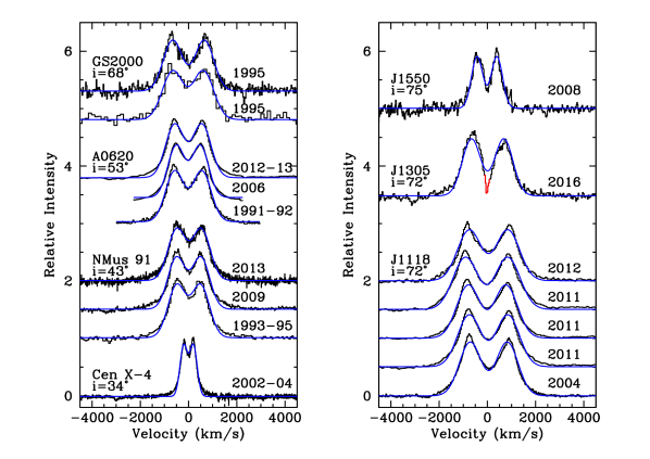
Figure 1: Orbital average H$\alpha$ spectra of our seven calibrators and their best 2-Gaussian model fits (blue). Different epochs/databases are shown for NMus 91, A0620, GS2000 and J1118. Binary inclinations are indicated for each source. In the case of the J1305 profile we mark in red the (masked) region contaminated by an interloper star (see Mata Sánchez et al. 2021).

In the case of the J1305 spectrum we followed Mata Sánchez et al. (2021) and mask part of the line core to remove the contamination produced by a well documented interloper star. In order to establish the optimal mask size we studied the impact of different widths on $T$ values, measured from a simulated profile with interloper contamination.This was constructed by adding a Gaussian absorption (with $FWHM=\Delta V_{\rm res}$ and centered at rest velocity) to the core of the J1118 H$\alpha$ line. The depth of the contaminating H$\alpha$ absorption is scaled to the interloper’s contribution as in Mata Sánchez et al. (2021). The choice of J1118 is motivated by the fact that both its spectral resolution and trough depth are nearly identical to those in J1305. By performing this test we find that the $T$ values obtained from the simulated profile are always larger than in the original J1118 spectrum, irrespectively of the size of the mask. The closest match is obtained for a mask width of 1.5$\times$$\Delta$$V_{\rm res}$, resulting in $T$ being overestimated by 0.012. We, therefore, decided to adopt a width mask of 1.5$\times$$\Delta$$V_{\rm res}$ in our fit to the J1305 profile and applied a small shift correction of -0.012 to the resulting $T$ value. We also increased the formal $T$ uncertainty by adding quadratically 0.012 in order to account for possible systematics introduced by the mask.

Regarding J1550, we note that the average spectrum is affected by limited phase coverage and thus, as shown in Appendix B, the $T$ measurement could be biased. However, the 16 individual spectra are evenly distributed around phases 0 and 0.7 (i.e. the minimum and maximum of the $T$ orbital modulation) and, therefore, we expect our $T$ determination not to differ much from its orbital average. Nonetheless, to account for possible systematics we have artificially increased the formal $T$ uncertainty (0.012) by adding quadratically 0.038 or 25 per cent of the amplitude expected from the orbital modulation.

The analysis of the Cen X-4 profile deserves further consideration. Cen X-4 is renowned for the presence of a very strong H$\alpha$ emission component, associated to the irradiated companion star (Torres et al., 2002; D’Avanzo et al., 2005, 2006). To minimize the impact of such component in the measurement of $T$ we produced a composite profile by merging two spectral halves with positive (red) and negative (blue) velocities. The blue part of the profile is obtained after co-adding VLT spectra taken at phases 0.1-0.4 (when the companion S-wave is located on the red peak) while the red profile is obtained from spectra within phases 0.6-0.9 (when it is placed on the blue peak). The 2-Gaussian model fit to the composite profile yields $T=0.147\pm 0.001$, but we realize this is an upper limit to the mean orbital value since our spectra sample phases close to the $T$ maxima (see Appendix B). A $T$ correction can be worked out by simulating a double sine-wave modulation of amplitude $\Delta T=\pm 0.15$ and maxima at phases 0.2 and 0.7. We find that the $T$ value obtained by sampling phases 0.1-0.4 and 0.6-0.9 results in an overestimate of the phase average by +0.06. On this ground, we correct our previous determination by -0.06 and adopt a conservative errorbar that encompasses it, i.e. $T=0.09\pm 0.06$.

Figure 2: Empirical correlation between the depth of the double peak trough ($T$) and binary inclination ($i$) for our seven calibrators. The open circle marks the position of Cen X-4.

The final list of $T$ values and inclinations for the seven calibration sources is given in Table 1 and plotted in Fig. 2. Note that Table 1 also provides the weighted mean of $T$ values (highlighted in bold face) for systems with multiple epochs. We regard these as the best possible determinations of trough depth since the effect of episodic variability is averaged out. A0620, N Mus 91 and J1118 contain the largest number of epochs (3-5), spanning over 1-2 decades, and henceforth we take their standard deviations as representative of the intrinsic variability in $T$ measurements of quiescent XRTs, i.e. $\Delta T\approx 0.02-0.03$. We also emphasize that the scaled-resolution parameter is $\Delta\lesssim 0.2$ in all cases thus implying that the $T$ values quoted in Table 1 are not affected by instrumental resolution (see Appendix A).

The points displayed in Fig. 2 draw a clear linear track. A least-squares linear fit with the newly scaled error bars yields

$$i(deg)=93.5(6.5)~{}T+23.7(2.5)$$ (4)

with a Pearson correlation coefficient $r=0.992$. In order to estimate the uncertainty in $i$ implied by this relation we have computed the difference with respect to the true observed inclinations for our seven calibrators. The distribution of differences is well fit by a normal function with $\sigma(i)=2^{\circ}$, which reflects the typical inclination uncertainty drawn by the correlation. Note here that we are not attempting to model a more physically motivated variation of $T$ with $\sin i$ because this follows a rather more complex (unknown) function than the simple linear correlation described by eq. 4. In any case, the calibration sample covers a wide range of inclinations between $i\sim 35-75^{\circ}$ and thus we believe our linear correlation is accurate at least within this interval.

5 Comparison with cataclysmic variables

For the sake of comparison, we have also obtained $T$ values for eight cataclysmic variables (CVs) from a database collected in Casares (2015). All the CVs are eclipsing and, therefore, possess very precise inclinations through light curve modeling of the white dwarf and/or hot-spot eclipses. The sample consists of three WZ Sge stars (WZ Sge itself, SDSS J103533.02+055158.3 - J1035 hereafter - and SDSS J143317.78+101123.3 - J1433 hereafter) which have large outburst amplitudes and decade-long recurrence times similar to XRTs. We also include five other more frequently outbursting dwarf novae: U Gem, HT Cas, OY Car, IP Peg and CTCV J1300-3052 (J1300 hereafter). For want of a better term, we refer to these five as dwarf novae as distinct from WZ Sge stars.

For the 2-Gaussian fit analysis we used orbital averages of the spectra reported in Table 2 of Casares (2015). It should be noted that the H$\alpha$ profile in J1035 is embedded in broad absorption wings, caused by superposition of the white dwarf spectrum. In this case, we removed the white dwarf contamination by subtracting a DA spectrum with $T_{\rm eff}=12000$ K and $\log g=8.0$, scaled to 85 per cent of the total flux (see Southworth et al. 2006) and degraded to the spectral resolution of J1035. Table 2 gives details of the CV spectra and fitting results, while Fig. 3 presents the data and model fits. A comparison of the measured CV trough depths with the $T-i$ correlation for XRTs is displayed in Fig. 4.

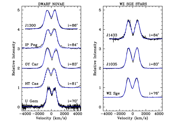
Figure 3: Symmetric 2-Gaussian fits to H$\alpha$ profiles of a sample of dwarf novae. The five (frequently outbursting) dwarf novae are shown in the left panel, while the right panel displays the three WZ Sge stars. Binary inclinations are indicated for each source.

Figure 4: Trough depth measured from a sample of CVs, compared to the $T-i$ correlation for XRTs (solid line). Open triangles mark the position of WZ Sge stars while asterisks those of the five dwarf novae.

Interestingly, we observe that trough depths in the five dwarf novae are systematically lower than predicted by the $T-i$ correlation By contrast, WZ Sge-type stars appear to fit well in the upper side of the correlation. Unfortunately, both the sample size and inclination range are too limited to draw any firm conclusion. Here we simply speculate with the possibility that non WZ Sge-type dwarf novae have too short outburst recurrence periods ($\sim$tens of days) for accretion discs to settle down in full quiescence. For example, the U Gem database was obtained 18 days after the end of a long outburst while the WZ Sge data $\sim$18 years past the previous 1978 outburst. For comparison, a 20 year monitoring campaign on the BH XRT V404 Cyg indicates that it takes $\approx$4 years for the accretion disc to shrink to a stable quiescence radius, as indicated by the evolution of the $FWHM$ and equivalent width of the H$\alpha$ line (Casares, 2015). Perhaps, frequently outbursting dwarf novae discs always display some level of activity in the form of outflow components (Matthews et al., 2015) that fill-in the line core and prevent unbiased determinations of the trough depth. In any case, more measurements from WZ Sge binaries over a wider range of (accurate) inclinations angles are required to probe whether their accretion discs do follow the $T-i$ correlation of XRTs.

6 Line profile modeling

In order to investigate the physical origin of the $T-i$ correlation in XRTs we have computed optically thick accretion disc line profiles for a range of inclinations. Following Orosz et al. (1994), we model the emission line profile of a flat axisymmetric Keplerian disc using the expression

$$F(u)\propto\int_{r_{1}}^{r_{z}}\frac{r^{3/2-\alpha}dr}{\left(1-u^{2}\,r\right)^{1/2}}\times\left[1+\left(2\,u\,\sin i\tan i\right)^{2}r\left(1-u^{2}\,r\right)\right]^{1/2},$$ (5)

where $r$ and $u$ are the dimensionless radius and radial velocity (i.e. normalized to the corresponding values at the outer edge of the disc), $r_{1}$ is the ratio of the inner to the outer disc radius and $r_{z}$=min (1, $u^{-2}$). Equation 5 assumes that the disc follows a power-law emissivity law of the form $f(r)=r^{-\alpha}$ (Smak, 1981), with previous works suggesting $\alpha\approx 1.5$ (Stover, 1981; Johnston et al., 1989; Horne & Saar, 1991). The inclination-dependent term of the equation accounts for the effect of shear broadening, which has been proposed to be the dominant local broadening contribution for $i\gtrsim 60^{\circ}$ (Horne & Marsh, 1986).

We start by simulating a synthetic profile for the canonical BH XRT A0620, where we adopt $i=53^{\circ}$ (Section 3). From our average GTC spectrum we estimate a peak velocity $DP/2=562$  km s^-1  and an extreme wing velocity set by the half-width-zero-intensity of the profile i.e. $HWZI=2500$  km s^-1. Assuming a Keplerian disc, with $DP/2$ and $HWZI$ corresponding to the outer and inner disc velocities respectively, we find $r_{1}=(562/2500)^{2}=0.05$. A synthetic A0620 profile was then computed from eq. 5 for $i=53^{\circ}$, $r_{1}=0.05$ and $DP/2=562$  km s^-1. The result was later convolved with a Gaussian of full-width at half-maximum $FWHM=140$  km s^-1 to simulate the instrumental resolution of the GTC spectrum. Fig. 5 shows the resolution-degraded profile (dotted line) compared to the GTC data. We immediately note that our synthetic model is much narrower than the data and needs to be broadened through additional convolution with a Gaussian of $FWHM$=361  km s^-1 (see Fig. 5). This quantity was derived through a $\chi^{2}$ minimization process on the residuals obtained after subtracting several broadened versions of the model from the observed profile. Stepping through the emissivity law exponent we also find that $\alpha=1.3$ provides a good description of the wings in the A0620 profile. The excess broadening that we find is not contemplated by eq. 5 and reflects some intrinsic (local) broadening that we dub $\Delta V_{\rm extra}$. We estimate a typical uncertainty of $\pm$15  km s^-1 in $\Delta V_{\rm extra}$ by varying $\alpha$ between 1-1.5 and $i$ in the range 50-55^∘.

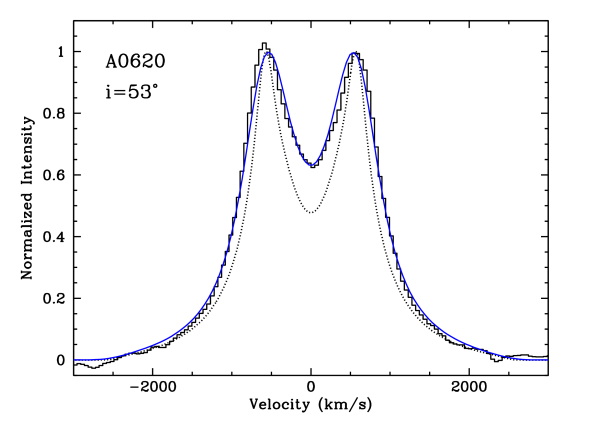
Figure 5: Orbital average GTC H$\alpha$ profile of A0620 (black histogram). The black dotted line represents an optically thick model computed from eq. 5 for $i=53^{\circ}$, $\alpha=1.3$, $r_{1}=0.05$ and $DP/2=562$  km s^-1, degraded to an instrumental resolution of 140  km s^-1. The blue continuous line depicts the same model but further broadened with a Gaussian of $FWHM$=361  km s^-1.

We subsequently produced a set of synthetic models with the very same parameters ($\alpha=1.3$, $r_{1}=0.05$, $\Delta V_{\rm extra}=361$  km s^-1) for a range of inclinations between 10^∘-90^∘ and extracted $T$ values by fitting the 2-Gaussian template introduced in Section 2. Note that we here assume that $\Delta V_{\rm extra}$ does not depend on binary inclination. For comparison, we also computed synthetic profiles with the same model but adopting $\Delta V_{\rm extra}=0$. Fig. 6 displays a selection of simulated profiles and template fits for the two broadening factors, while Fig. 7 (top panel) presents the $T-i$ evolution derived from the fits. The latter figure shows that the synthetic $T-i$ correlation provides a good description of the empirical data if, and only if, the appropriate excess line broadening is taken into account. As a matter of fact, neglecting or underestimating $\Delta V_{\rm extra}$ leads to $T$ values that are systematically larger than those predicted by the correlation. The figure also evinces an obvious limitation of the technique: the inability to measure low inclinations $i\lesssim 30^{\circ}$ due to the disappearance of the double peak (see e.g. the $i=20^{\circ}$ profile in the left panel of Fig. 6). This occurs when $W$ approaches $DP$ due to either a high intrinsic broadening $\Delta V_{\rm extra}$, poor spectral resolution or both, situation that translates into large values of the scaled-resolution parameter $\Delta$ (see Appendix A).

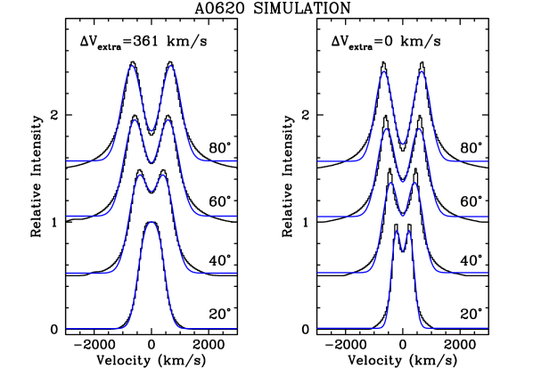
Figure 6: 2-Gaussian model fits (blue) to synthetic optically thick disc profiles of A0620 for a range of inclinations. All profiles have been convolved with a Gaussian of 140  km s^-1 to account for instrumental resolution. Left panel depicts models with added line broadening $\Delta V_{\rm extra}=361$  km s^-1 while the right panel those with no extra broadening.

Since $\Delta V_{\rm extra}$ may vary from system to system we decided to compute synthetic models for Cen X-4 and J1118 as well. These binaries were selected because present us with the narrowest and broadest H$\alpha$ profiles within our sample of calibrators. As for A0620, optically thick line models were computed for Cen X-4 ($i=34^{\circ}$, $\alpha=1.5$, $r_{1}=0.05$) and J1118 ($i=72^{\circ}$, $\alpha=1.3$, $r_{1}=0.12$). Optimal line broadenings were derived through comparison of the resolution-degraded synthetic models with the observed profiles. These were found to be $\Delta V_{\rm extra}=141\pm 14$  km s^-1 and $465\pm 40$  km s^-1 for Cen X-4 and the GTC J1118 spectra, respectively. Again, the uncertainties in $\Delta V_{\rm extra}$ were inferred by varying $\alpha$ in the range 1-1.5 and $i$ between the allowed limits (see Table 1). Synthetic $T-i$ correlations were subsequently produced by fitting the broadened model profiles, computed for a range of inclinations, with the 2-Gaussian template. The bottom panel in Fig. 7 presents the resulting synthetic $T-i$ correlations. The plot shows that, despite of the very different $\Delta V_{\rm extra}$ broadenings (141 and 465  km s^-1) the two new simulations still provide a good description of the data in the entire range.

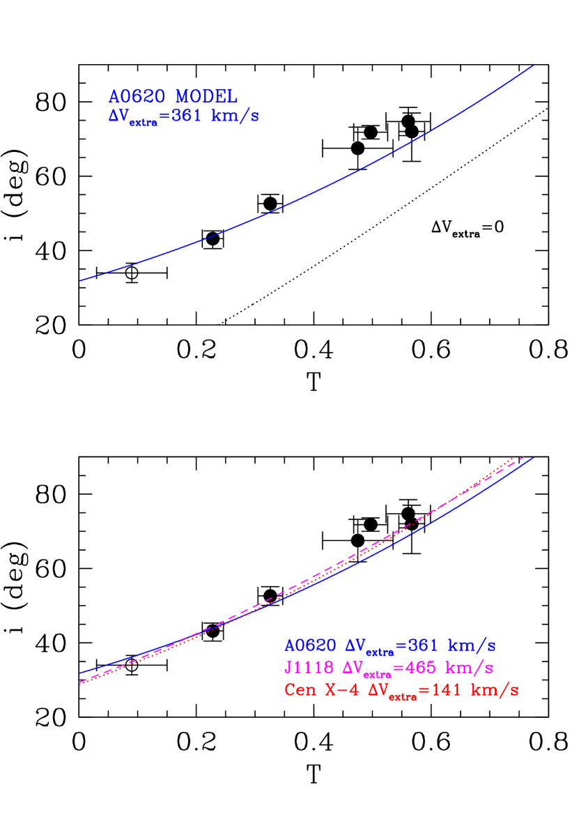
Figure 7: Top: synthetic $T-i$ correlation obtained from an optically thick line model for A0620 with extra broadening $\Delta V_{\rm extra}=361$  km s^-1(blue line). The black dotted line depicts the same model with $\Delta V_{\rm extra}=0$. For comparison we overplot the data points of the calibration sample, using the same symbols as in Fig. 2. Bottom: same for model profiles of Cen X-4 (red dotted line) and J1118 (magenta dashed line), with excess line broadening $\Delta V_{\rm extra}=141$ and 465  km s^-1 respectively.

In summary, we have seen that, notwithstanding obvious limitations at very low inclination angles, the presence of some excess broadening, in addition to line opacity, plays a fundamental role in shaping the line profiles and producing the tight $T-i$ correlation that we observe. Every system possesses a characteristic $\Delta V_{\rm extra}$ that, if not properly accounted for, would blur the correlation by providing overestimated $T$ values.

6.1 Excess broadening

So far we have made the first-order approximation that $\Delta V_{\rm extra}$ is isotropic, i.e. independent from binary inclination. Since our calibration database spans a wide range of inclination angles and outer disc velocities it presents us with the opportunity to further characterize $\Delta V_{\rm extra}$. We thus computed synthetic optically thick line models for the remaining four XRT calibrators at their corresponding inclinations and, as before, derived extra line broadenings for each case. In order to extend the sample to even larger disc velocities we also included an orbital-averaged GTC spectrum of Swift J1357-0933 (hereafter referred to as J1357) from Mata Sánchez et al. (2015), where we adopt $i=87^{\circ}$ (see Section 7). In all the cases we find good line fits for $\alpha=1-1.5$ and $r_{1}$ in the range 0.05-0.13. Table 3 lists the optimal excess broadenings obtained for these model profiles ($\Delta V_{\rm extra}$), together with their outer disc velocities that we assume close to Keplerian, i.e. $V_{\rm Kep}\approx DP/(2\sin i)$. For comparison, we also list the expected values for thermal and shear broadening, given by $\Delta V_{\rm th}\sim V_{\rm Kep}~{}(H/R)$ and $\Delta V_{\rm shear}\sim\Delta V_{\rm th}~{}\sin i~{}\tan i$ (Horne & Marsh, 1986), where $R$ and $H$ stand for the outer disc radius and elevation, respectively. Here we have adopted a typical thin disc aspect ratio $H/R\sim 0.05$. In the case of systems with several epochs we have computed $\Delta V_{\rm extra}$ for each epoch individually and find very stable values, with typical variations in the range $\sim 10-30$  km s^-1 and always smaller than the uncertainty associated with the choice of model parameters.

Table 3 shows that $\Delta V_{\rm extra}$ is much larger than shear broadening, except for J1357. The latter is likely a consequence of the $\Delta V_{\rm shear}$ expression breaking down at very extreme lines of sight $\tan i\gtrsim R/H$ (i.e. $i\gtrsim 87^{\circ}$). As a matter of fact, $\Delta V_{\rm extra}$ appears to correlate well with the outer disc velocity (see top panel in Fig. 8) but not binary inclination. In particular, four XRTs with a wide range of inclinations $i=43-72^{\circ}$ (N Mus 91, A0620, GS2000 and J1305) possess very similar $\Delta V_{\rm extra}$ and $V_{\rm Kep}$ values. Furthermore, J1550, despite its high inclination, has low $\Delta V_{\rm extra}$ and $V_{\rm Kep}$ values, comparable to those of the low-inclination binary Cen X-4. A least-squares linear fit to the distribution of $\Delta V_{\rm extra}$ and $V_{\rm Kep}$ values yields

$$\Delta V_{\rm extra}=0.65~{}V_{\rm Kep}-94.$$ (6)

Interestingly, eq. 6 offers an alternative route to obtain a rough estimate of the binary inclination by simply comparing the double peak separation with $V_{\rm Kep}$. For practical reasons, it is convenient to express line broadenings in terms of the $W$ values supplied by the 2-Gaussian template, which are listed in Table  1. A linear fit (see bottom panel in Fig. 8) gives

$$\Delta V_{\rm extra}=0.41~{}W$$ (7)

and, since $V_{\rm Kep}\approx DP/(2~{}\sin i)$, then $i\approx\arcsin[DP/(289+1.25~{}W)]$. Comparing the inclinations derived from this expression with those listed in Table  1 for the seven calibrators we find that the latter can be recovered with a typical uncertainty of $\approx$4 deg.

Figure 8: Top panel: Excess line broadening measured in eight XRTs versus deprojected outer disc velocities. The linear fit $\Delta V_{\rm extra}=0.65~{}V_{\rm Kep}-94$ is also shown. Bottom panel: same versus the intrinsic width of the 2-Gaussian template model. A linear fit $\Delta V_{\rm extra}=0.41~{}W$ is overplotted.

Furthermore, since $V_{\rm Kep}$ is set by the central object’s mass and outer disc radius (which in turn depends on the orbital period), $\Delta V_{\rm extra}$ is ultimately determined by fundamental binary parameters. Therefore, one can use $W$ to directly constrain the binary period and mass of the compact star. To do so we assume that the disc is truncated at the 3:1 resonance radius $R=3^{-2/3}\left(1+q\right)^{-1/3}a$ (Frank, King & Raine, 2002), where $a$ is the binary separation and $q=M_{2}/M_{1}$ the companion star to compact object mass ratio. On the other hand, the outer disc velocity is given by $V_{\rm Kep}=\beta\left(\frac{GM_{1}}{R}\right)^{1/2}$, where $\beta$ is a correction factor that accounts for the fact that the outer disc material is sub-Keplerian, due to tidal interaction with the companion star. After some algebra, where we bring in Kepler’s third Law and eqs. 6 and 7, we find

$$M_{1}^{\ast}=3.45\times 10^{-8}~{}P_{\rm orb}~{}[\left(0.63~{}W+145\right)/\beta]^{3}~{}~{}~{}~{}~{}M_{\odot},$$ (8)

where $P_{\rm orb}$ is the orbital period in days and $W$ is given in  km s^-1. This equation is rather powerful as it allows the measurement of compact object masses directly from the width of the line profile, provided that $P_{\rm orb}$ is known (or vice versa). And this can be exploited without any prior information on dynamical parameters, the binary mass ratio or inclination. It is worth mentioning that $\Delta V_{\rm extra}$ has been obtained for the H$\alpha$ line and, therefore, eqs. 6-8 should not be applied to other transitions since it has been shown that broadening varies between lines (e.g. van Spaandonk et al. 2010).

As an example, we have applied eq. 8 to our list of calibrators and compared the results with dynamical masses reported in literature. As we did for the inclination angle (see Section 3), we here adopt the unweighted mean of the masses reported by independent studies with credible inclination determinations. For comparison purposes, we have also included the three WZ Sge-type CVs from Section 5. The best match between $M_{1}^{\ast}$ and the dynamical mass $M_{1}$ is obtained for $\beta=0.84$, in good agreement with other studies that suggest outer disc velocities are sub-Keplerian by $\approx$20 per cent (e.g. Wade & Horne 1988; Casares 2016). The results are listed in Table 4 and displayed in Fig. 9. The distribution of differences indicates that eq. 8 allows recovering dynamical masses with a $\sim$20 per cent accuracy, which is sufficient to separate BHs from other compact stars such as neutron stars (NSs) and white dwarfs.

To summarize this section, we have shown that optically thick line models can reproduce the observed profiles in XRTs only if an extra source of line broadening (surpassing shear broadening) is included. The origin of this supersonic broadening is unclear, with Stark broadening (Marsh & Dhillon, 1997) or dynamo effects in a magnetically dominated disc (Armitage et al., 1996) as possible options. A full discussion of the nature of the excess broadening is beyond the scope of this paper, although we note that $\Delta V_{\rm extra}$ increases linearly with the outer disc velocity. It is the mere existence of such scaling, together with line opacity, that allows explaining the observed $T-i$ correlation. In other words, for a given binary, the ratio $M_{1}/P_{\rm orb}$ establishes the outer disc velocity $V_{\rm Kep}$ which in turn defines both $DP/\sin i$ and $W$, the essential ingredients of the correlation. As a corollary, the scaling between excess broadening and outer disc velocity permits deriving fundamental binary parameters by simply resolving the width of the double peak emission profile (eq. 8).

Figure 9: Dynamical masses ($M_{1}$) of the seven calibrators versus masses derived from line profile broadenings through eq. 8, with $\beta=0.84$ ($M_{1}^{\ast}$). We also display the three WZ Sge CVs from Sect. 5. Same symbols are used as in Figs. 2 and 4. The maximum NS and Chandrasekhar mass limits are indicated for comparison.

7 Application of the $T-i$ correlation

Having presented the $T-i$ correlation and its implications, we can now exploit eq. 4 and derive binary inclination angles for BHs with poor or disputed determinations. This is mainly the case of binaries where the companion’s light curve is heavily veiled/contaminated by strong flickering. As an example, we apply the technique to the XRTs J1357 and GRO J0422+32 (=V518 Per; hereafter J0422).

J1357 is characterized by huge flickering variability, with amplitudes up to 1.5 mag that totally conceal the companion’s ellipsoidal modulation (Shahbaz et al., 2013). Based on (i) the presence of optical dips, (ii) an extremely broad H$\alpha$ profile and (iii) a low outburst X-ray luminosity, Corral-Santana et al. (2013) proposed that the source is seen at very high (nearly edge-on) inclination $i\gtrsim 80^{\circ}$. Further support for an extreme binary geometry was provided by observations of deep absorption cores in the H$\alpha$ and HeI $\lambda$5876 emission lines (Mata Sánchez et al., 2015). This interpretation was however disputed by Armas Padilla et al. (2014) and Beri et al. (2019) through the lack of high-inclination spectral and timing X-ray features (see also Torres et al. 2015).

In the case of J0422, the optical light curves are severely distorted by large flickering variability, with amplitudes of up to 0.6 mag. As a result, attempts to model the barely detectable ellipsoidal modulation by different groups have resulted in a wide range of inclination angles $i=10-49^{\circ}$ (Casares et al., 1995b; Callanan et al., 1996a; Beekman et al., 1997; Webb et al., 2000; Gelino & Harrison, 2003; Reynolds et al., 2007).

In order to derive H$\alpha$ line trough depths we have produced orbital averages for the two binaries. We used 42 GTC spectra of J1357 at 800  km s^-1 resolution, reported in Mata Sánchez et al. (2015) and 18 unpublished GTC spectra of J0422, obtained in 2016 Jan 9 at 360  km s^-1 resolution, both covering a complete orbital cycle. A thorough analysis of the latter spectra will be presented elsewhere (González Hernández et al. in preparation). Fig. 10 displays the average GTC spectra and 2-Gaussian model fits for the two systems. We find $T=0.683\pm 0.006$ and $0.341\pm 0.007$ for J1357 and J0422 respectively. It should be stressed that, as before, the $T$ values have been obtained by fitting a 2-Gaussian model that has been degraded to the instrumental resolution of each database. In addition, because of the large scaled-resolution parameters ($\Delta=0.42$ and 0.69) we apply a small correction through eq. 10, which translates into +0.017 for J1357 and +0.046 for J0422. Finally, since the $T$ measurements are based on single epoch observations, we decide to adopt a typical uncertainty $\sigma(T)=0.025$ (i.e. a factor 4 larger than the formal error) so to account for the effect of possible intrinsic variability (see Sect. 4). The final fitting results are presented in Table 5. The trough depths measured imply $i=87.4^{+2.6}_{-5.6}$ deg and $55.6\pm 4.1^{\circ}$ for J1357 and J0422, respectively, where the uncertainties have been derived through a Monte Carlo simulation with $10^{5}$ realizations.

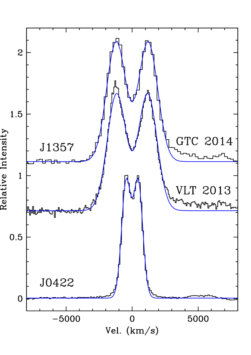
Figure 10: 2-Gaussian model fits to orbital averaged spectra of J0422 and two epochs of J1357: VLT 2013 and GTC 2014. The red wing of J1357 (velocities between 3000-8000  km s^-1) is contaminated by HeI $\lambda$6678 emission and has been masked from the fit.

We note that our new J0422 inclination is higher than previous estimates (with closest matches provided by Casares et al. 1995b and Gelino & Harrison 2003) although lower than the $63.7\pm 5.2^{\circ}$ value inferred by Kreidberg et al. (2012), after correcting for flickering systematics with a model based on the A0620 disc contamination. The inclination of J1357, on the other hand, agrees well with Corral-Santana et al. (2013) and Mata Sánchez et al. (2021), thus supporting a near edge-on geometry for this binary. We warn, however, that the J1357 inclination should be taken with some caution because it is based on extrapolating the $T-i$ correlation beyond the $i=35-75^{\circ}$ domain where it has been tested. Even if we were to believe the $T$ values of the WZ Sge stars, J1357 is placed at higher inclinations, where the $T-i$ correlation is likely to break down because of extreme lines of sight $\tan i\gtrsim R/H$, comparable to the disc aspect ratio.

As a test, we have also fitted the average of 24 medium resolution (229  km s^-1) VLT spectra of J1357 obtained in 2013 (Torres et al., 2015). The spectra cover 84 per cent of an orbital cycle. The 2-Gaussian fit yields $T=0.503\pm 0.025$ which translates into $i=70.6\pm 4.7^{\circ}$ (see Fig. 10). This is significantly different than the values obtained from the 2014 GTC spectra. Most of the discrepancy can be ascribed to the larger excess broadening of the VLT spectra, that we estimate to be 1020  km s^-1. Furthermore, we note that the VLT data were collected only 1.6 years after the end of the 2011 outburst, compared to 2.8 years for the GTC data. Based on the larger excess broadening and close outburst proximity we interpret that the 2013 VLT spectra were obtained when the accretion disc did not yet reach complete quiescence and, therefore, give more credit to the GTC result. The outlier behaviour of the J1357 VLT spectra is further supported by multi-epoch observations of XTE J1859+226, where both $T$ and excess broadening measurements obtained from data collected seven years apart show very consistent values, with deviations of only 0.04 and 12 km/s, respectively (Yanes-Rizo et al. 2022, submitted). In any case, a more conservative estimate of the inclination in J1357 is provided by the weighted average of $T$ values from the two independent epochs, which results in $T=0.612\pm 0.125$ and thus $i=81^{+9}_{-12}$ deg.

8 Discussion: Updated BH masses and implications

Armed now with the newly derived inclinations we can revise the BH masses in J0422 and J1357 using the observable

$$M_{1}=f(M)\times\frac{(1+q)^{2}}{\sin^{3}i}$$ (9)

where $f(M)={K_{2}^{3}P_{\rm orb}\over{2\pi G}}$ is the mass function of the compact star. In order to derive $M_{1}$ and its uncertainty we have run Monte Carlo simulations with 10⁵ realizations. We have adopted Gauss-normal distributions for $K_{2}$, $P_{\rm orb}$ and $q$, as reported in literature, together with our recent $i$ determinations (also normally distributed). The adopted values and associated references are listed in Table 6. Fig. 11 presents the probability density functions of the two BH masses, with the median values and uncertainties also given in Table 6.

Remarkably, we find $M_{1}=2.7^{+0.7}_{-0.5}$ M_⊙ (68 per cent) for J0422. The BH mass lies under 5 M_⊙ with 99.5 per cent confidence, robustly placing it within the so-called "mass gap" that separates NSs from BHs (Bailyn et al., 1998; Özel et al., 2010; Farr et al., 2011). Incidentally, the companion’s mass implied by this $M_{1}$ and a well constrained mass ratio (Table 6) is $M_{2}=q~{}M_{1}=0.33^{+0.28}_{-0.20}$ M_⊙, in excellent agreement with the observed M0-5 V spectral type classification (Orosz & Bailyn, 1995; Casares et al., 1995b; Harlaftis et al., 1999; Webb et al., 2000). On the other hand we obtain $M_{1}=10.9^{+1.7}_{-1.6}$ M_⊙ for J1357 ($M_{1}=11.6^{+2.5}_{-1.9}$ M_⊙ if we adopt a more conservative inclination $i=81^{+9}_{-12}$ deg), which establishes it as one of the most massive BH XRTs in the Galaxy, only comparable to GRS 1915+105 (Reid et al., 2014). It is interesting to note the good agreement between these BH masses and those inferred directly from the width of the 2-Gaussian model fit, coupled with $P_{\rm orb}$ (i.e. $M_{1}^{\ast}$ in Table 4).

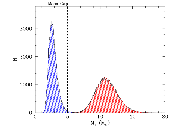
Figure 11: The BH mass probability distributions for J0422 (blue) and J1357 (red) derived from Monte Carlo simulations with 10⁵ trials. The vertical dashed lines mark the limits of the mass gap between NSs and BHs.

The evidence of a low-mass BH in J0422 has strong implications for BH formation theories. Several models have been put forward to explain the apparent dearth of BHs with masses between 2-5 M_⊙, including fast convection instabilities (Belczynski et al., 2012), neutrino-driven explosions (Ugliano et al., 2012) or red supergiant failed supernovae (Kochanek, 2014). Other core collapse simulations though, predict a continuous distribution of compact remnants (e.g. Fryer & Kalogera 2001) or the existence of a less populated region under $\approx$6 M_⊙ but without a real gap (Ertl et al., 2020). Recent observations of microlense events also favour a continuous distribution of remnant masses (Wyrzykowski & Mandel, 2020). A light BH in J0422 strongly disproves the existence of a mass discontinuity between NSs and BHs, lending support to formation scenarios through fallback in weak supernova explosions (Ertl et al., 2020; Woosley et al., 2020) and/or accretion-induced collapse of NSs (Vietri & Stella, 1999; Dermer & Atoyan, 2006; Gao et al., 2022). Further, it suggests that the apparent lack of 2-5 M_⊙ BHs is not necessarily driven by supernova physics but, instead, could be an artifact of low number statistics, selection biases and possible systematics associated with the measurement of inclination angles (see Kreidberg et al. 2012).

Other examples of low-mass BH candidates that may fall into the gap are MWC656 (Casares et al., 2014), 2M05215658+4359220 (Thompson et al., 2019) and V723 Mon (Jayasinghe et al., 2021), although none presents such a clear-cut case as J0422 (e.g. see BH imposter scenarios in van den Heuvel & Tauris 2020 and El-Badry et al. 2022). Note that, at variance with these other candidates, J0422 was discovered through an accretion-driven outburst and showed X-ray properties that are characteristic of dynamically confirmed BHs, namely (1) a hard power-law spectrum extending beyond 100 keV (Sunyaev et al., 1993), (2) a gamma-ray excess at 1-2 MeV (Roques et al., 1994; van Dijk et al., 1995) and (3) the presence of low frequency QPOs (Kouveliotou et al., 1993; Vikhlinin et al., 1995; van der Hooft et al., 1999).

Our result on J0422 also impacts the interpretation of gravitational wave (GW) mergers at the low-mass end. For example, GW190425 is believed to result from a binary NS coalescence but its total mass (3.4${}^{+0.3}_{-0.1}$ M_⊙) stands clearly above the mean in the distribution of Galactic binary NSs (Abbott et al., 2020a) and hence the possibility that one of the compact stars was a low-mass BH cannot be dismissed (Han et al., 2020; Foley et al., 2020). Similarly, the analysis of GW190814 implies the merger of a 22.2-24.3 M_⊙ BH with a 2.50-2.67 M_⊙ compact star of uncertain nature (Abbott et al., 2020b). GW200105 and GW200210, recently disclosed by the GWTC-3 catalogue, also reveal coalescence of BHs with companions of 1.91${}^{+0.33}_{-0.24}$ M_⊙ and 2.83${}^{+0.47}_{-0.42}$ M_⊙, that could be either massive NSs or light BHs (see Abbott et al. 2021 and references therein). In principle, the two scenarios could be distinguished from the imprint of the tidal deformability of the NS in the GW signal but unfortunately this will not be possible before third generation detectors become operative beyond $\sim$2044 (Chen et al., 2020). Meanwhile, the evidence of a BH in J0422 with a mass of $2.7^{+0.7}_{-0.5}$ M_⊙ strengthens the possibility that low-mass BHs might be present in some GW events.

9 Conclusions

We have shown that the depth of the trough ($T$) in double-peaked H$\alpha$ lines from XRT discs is linearly correlated with the inclination angle. This is a natural consequence of line opacity and local broadening, where a new broadening process (exceeding shear broadening) plays a leading role. The here called $T-i$ correlation opens a new avenue to derive binary inclinations (and therefore masses) in quiescent XRTs, in particular when ellipsoidal light curves are swamped or contaminated by strong flickering. Data with sufficient orbital coverage ($\gtrsim$50 per cent) and spectral resolution ($\Delta V_{\rm res}\lesssim 0.5\sqrt{DP^{2}-W^{2}}$) are nevertheless required to prevent $T$ values (and inclinations) from being affected by systematic biases.

We also find that the line excess broadening is proportional to the outer disc velocity. Such scaling allows inferring the ratio $M_{1}/P_{\rm orb}$ directly from the line broadening, without prior knowledge of other fundamental parameters (binary mass ratio, companion’s velocity or inclination). Therefore, if the orbital period is known, compact object masses can be estimated (to $\approx$20 per cent accuracy) by simply resolving the intrinsic width of the H$\alpha$ line (and viceversa).

We applied the $T-i$ correlation to J0422 and J1357, two BHs with poor inclination constraints due to heavy flickering contamination. We find $i=55.6\pm 4.1^{\circ}$ and $87.4^{+2.6}_{-5.6}$ deg which lead to $M_{1}=2.7^{+0.7}_{-0.5}$ M_⊙ and $10.9^{+1.7}_{-1.6}$ M_⊙ (68 per cent confidence), respectively. The BH in J0422 is robustly placed within the 2-5 M_⊙ mass gap that divides NSs from BHs, proving that low-mass BHs do exist in nature and can be formed through stellar evolution in X-ray binaries. This argues for the mass gap being produced by limited statistics and observational biases rather than the physics of core collapse supernovae. The result on J0422 also brings new support to the possibility that the light companions in the GW190814 and GW200210 mergers (perhaps also GW200105) were low-mass BHs. Finally, the $T-i$ correlation presented here opens the possibility to substantially expand the census of accurate BH masses and revisit the mass distribution of stellar BHs in the Galaxy. We are currently working on this project.

10 Data availability

All data used in this article is publicly available from the relevant observatory archives. The data will be shared on reasonable request to the corresponding author.

Table 1: Calibration binaries

Target	Date	Telescope	$\Delta V_{\rm res}$	Phase Coverage	$DP$	$W$	$\Delta^{\S}$	$T$	$i$	References
			(km/s)		(km/s)	(km/s)			(deg)	for $i$
Cen X-4	2002-04	VLT	7	33%	404.70$\pm$0.03	364.92$\pm$0.05	0.04	0.090$\pm$0.060 †	34.0$\pm$2.6	1-3
N Mus 91	Average	-	-	-	-	-	-	0.228$\pm$0.018	43.2${}^{+2.1}_{-2.7}$	4
Epoch 1	1993-95	NTT	90	100%	989.0$\pm$3.8	860.6$\pm$5.4	0.18	0.199$\pm$0.011
Epoch 2	2009	Magellan	46	75%	1009.4$\pm$2.1	855.2$\pm$3.0	0.09	0.238$\pm$0.006
Epoch 3	2013	VLT	43	70%	1015.7$\pm$3.2	869.8$\pm$4.5	0.08	0.223$\pm$0.009
A0620	Average	-	-	-	-	-	-	0.326$\pm$0.021	52.6$\pm$2.5	5-6
Epoch 1	1991-92	WHT	70	100%	1126.6$\pm$0.02	893.7$\pm$0.03	0.10	0.335$\pm$0.001
Epoch 2	2006	Magellan	130	100%	997.8$\pm$0.2	809.8$\pm$0.2	0.19	0.302$\pm$0.001
Epoch 3	2012-13	GTC	140	100%	1122.9$\pm$0.3	887.7$\pm$0.4	0.20	0.340$\pm$0.001
GS2000	Average	-	-	-	-	-	-	0.475$\pm$0.060	67.5$\pm$5.7	7-8
Epoch 1	22/07/1995	Keck	120	100%	1303.8$\pm$10.0	928.5$\pm$12.3	0.13	0.490$\pm$0.021
Epoch 2	25-27/07/1995	WHT	196	100%	1262.6$\pm$25.4	986.5$\pm$34.3	0.22	0.358$\pm$0.059
J1118	Average	-	-	-	-	-	-	0.497$\pm$0.029	71.8$\pm$1.8	9-11
Epoch 1	2004	Keck	50	100%	1535.9$\pm$1.8	1062.8$\pm$2.1	0.05	0.530$\pm$0.003
Epoch 2	07/02/2011	GTC	120	100%	1596.6$\pm$1.3	1130.2$\pm$1.6	0.11	0.498$\pm$0.002
Epoch 3	08/02/2011	GTC	120	100%	1557.7$\pm$1.0	1126.0$\pm$1.2	0.11	0.469$\pm$0.002
Epoch 4	25/04/2011	GTC	120	100%	1745.1$\pm$1.6	1206.8$\pm$1.9	0.11	0.531$\pm$0.002
Epoch 5	12/01/2012	GTC	120	100%	1596.0$\pm$3.2	1151.5$\pm$4.0	0.11	0.472$\pm$0.006
J1305	2013	VLT	140	100%	1339.2$\pm$4.7	893.9$\pm$5.9	0.14	0.567$\pm$0.022 ††	72.0${}^{+5.0}_{-8.0}$	12
J1550	2008	Magellan	55	30%	817.3$\pm$3.7	552.5$\pm$4.3	0.09	0.561$\pm$0.038 †††	74.7$\pm$3.8	13

References: (1) Khargharia et al. (2010), (2) Shahbaz et al. (2014), (3) Hammerstein et al. (2018), (4) Wu et al. (2016), (5) Cantrell et al. (2010), (6) van Grunsven et al. (2017), (7) Callanan et al. (1996b), (8) Ioannou et al. (2004), (9) Gelino et al. (2006), (10) Khargharia et al. (2013), (11) Cherepashchuk et al. (2019), (12) Mata Sánchez et al. (2021) and (13) Orosz et al. (2011)
^§ Scaled-resolution parameter, defined as $\Delta=\Delta V_{\rm res}/\sqrt{DP^{2}-W^{2}}$.
^† $T$ value and error corrected for orbital phasing.
^†† $T$ value corrected by -0.012 and formal error increased by +0.012 to account for masking the contamination of an interloper star in the line core.
^††† An overall error of 0.038 has been adopted to account for the possible effect of orbital variability.

Table 2: Cataclysmic variables

Target	CV type	$\Delta V_{\rm res}$	Phase Coverage	$DP$	$W$	$\Delta$	$T$	$i$	References
		(km/s)		(km/s)	(km/s)			(deg)	for spectra & $i$
U Gem	Dwarf novae	16	100%	908.7$\pm$1.0	726.0$\pm$1.3	0.03	0.325 $\pm$0.003	69.7$\pm$ 0.7	1,2
HT Cas	,,	120	60%	1089.4$\pm$2.9	922.3$\pm$4.0	0.21	0.230$\pm$0.007	81.0$\pm$1.0	3,4
OY Car	,,	46	100%	1296.6$\pm$0.3	942.2$\pm$0.4	0.05	0.462$\pm$0.001	83.3$\pm$0.2	5,6
IP Peg	,,	150	100%	1066.7$\pm$4.6	899.9$\pm$6.5	0.26	0.245$\pm$0.012	83.8$\pm$0.2	7,8
J1300	,,	45	100%	1164.6$\pm$0.7	900.7$\pm$0.9.	0.06	0.372$\pm$0.002	85.7$\pm$1.5	9
WZ Sge	WZ Sge	25	100%	1223.9$\pm$0.6	835.2$\pm$0.7	0.03	0.549$\pm$0.001	75.9$\pm$0.3	10,11
J1035	,,	69	100%	1254.8$\pm$1.5	809.6$\pm$1.7	0.07	0.622$\pm$0.003	83.1$\pm$0.2	6,12
J1433	,,	32	100%	1368.5$\pm$2.4	826.9$\pm$2.7	0.03	0.700$\pm$0.004	84.2$\pm$0.2	6,13

References: (1) Echevarría et al. (2007), (2) Zhang & Robinson (1987), (3) Casares (2015), (4) Horne, Wood & Stiening (1991), (5) Copperwheat et al. (2012) (6) Littlefair et al. (2008), (7) Harlaftis et al. (1994), (8) Copperwheat et al. (2010), (9) Savoury et al. (2012), (10) Skidmore et al. (2000), (11) Skidmore et al. (2002), (12) Southworth et al. (2006), (13) Tulloch et al. (2009)

Table 3: Sources of local line broadening in 8 XRTs

Target	$i$	$V_{\rm Kep}$	$\Delta V_{\rm extra}$	$\Delta V_{\rm th}$	$\Delta V_{\rm shear}$
	(deg)	(km/s)	(km/s)	(km/s)	(km/s)
Cen X-4	34	362	141$\pm$14	18	7
N Mus 91	43	725	338$\pm$47	36	23
A0620	53	703	361$\pm$15	35	37
GS2000	68	703	328$\pm$72	35	80
J1118	72	855	465$\pm$40	43	125
J1305	72	704	415$\pm$63	35	103
J1550	75	423	196$\pm$36	21	76
J1357	87	1211	740$\pm$90	61	1089

Table 4: Compact objects masses from line broadenings ($M_{1}^{\ast}$) compared to dynamical masses ($M_{1}$)

Target	$P_{\rm orb}$	$W$	$M_{1}^{\ast}$	$M_{1}$	References
	(d)	(km/s)	(M⊙)†	(M⊙)	for $M_{1}$
Cen X-4	0.6290522(4)	364.92$\pm$0.05	1.93$\pm$0.001	1.64$\pm$0.31	1-3
N Mus 91	0.43260249(9)	860.6$\pm$5.4	8.16$\pm$0.12	11.0${}^{+2.1}_{-1.4}$	4
A0620	0.32301405(1)	887.7$\pm$0.4	6.56$\pm$0.01	6.23$\pm$0.17	5-6
GS2000	0.3440915(9)	928.5$\pm$12.3	7.78$\pm$0.24	7.82$\pm$0.89	7-8
J1118	0.16993404(5)	1159.2$\pm$0.9	6.63$\pm$0.01	7.76$\pm$0.40	9-11
J1305	0.394(4)	893.9$\pm$5.9	8.14$\pm$0.12	8.9${}^{+1.6}_{-1.0}$	12
J1550	1.5420333(24)	552.5$\pm$4.3	10.75$\pm$0.17	9.10$\pm$0.61	13
WZ Sge	0.0566878460(3)	835.2$\pm$0.7	0.997$\pm$0.002	0.740$\pm$0.071	14
J1035	0.0570067(2)	760.0$\pm$1.2	0.805$\pm$0.003	0.94$\pm$0.01	15
J1433	0.054240679(2)	826.9$\pm$2.7	0.931$\pm$0.007	0.868$\pm$0.007	15

References: (1) Khargharia et al. (2010), (2) Shahbaz et al. (2014), (3) Hammerstein et al. (2018), (4) Wu et al. (2016), (5) Cantrell et al. (2010), (6) van Grunsven et al. (2017), (7) Callanan et al. (1996b), (8) Ioannou et al. (2004), (9) Gelino et al. (2006), (10) Khargharia et al. (2013), (11) Cherepashchuk et al. (2019), (12) Mata Sánchez et al. (2021), (13) Orosz et al. (2011), (14) Skidmore et al. (2002), (15) Littlefair et al. (2008)
^† $M_{1}^{\ast}$ is obtained from eq. 8, with $\beta=0.84$. Quoted errors are pure formal uncertainties.

Table 5: Profile fit parameters and inclinations in 2 BH XRTs

Target	$\Delta V_{\rm res}$	Phase Coverage	$DP$	$W$	$\Delta$	$T^{\dagger}$	$i$
	(km/s)		(km/s)	(km/s)			(deg)
J1357	800	100%	2418.5$\pm$4.6	1504.6$\pm$6.4	0.42	0.683$\pm$0.025	87.4${}^{+2.6}_{-5.6}$
J0422	360	100%	908.0$\pm$2.1	740.5$\pm$3.3	0.69	0.341$\pm$0.025	55.6$\pm$4.1

^† Because of the large $\Delta$ values the quoted $T$ have been corrected for instrument resolution degradation using eq. 10.

Table 6: Fundamental parameters and dynamical masses for 2 BH XRTs

Target	$P_{\rm orb}$	$K_{2}$	$q$	$i$	$M_{1}$	$M_{1}^{\ast}$	References
	(d)	(km/s)		(deg)	(M⊙)	(M⊙)†
J1357	0.106969(23)	967$\pm$49	0.039$\pm$0.004	87.4${}^{+2.6}_{-5.6}$	10.9${}^{+1.7}_{-1.6}$	8.1$\pm$1.6	1-3
J0422	0.2121600(2)	378$\pm$16	0.12$\pm$0.08	55.6$\pm$4.1	2.7${}^{+0.7}_{-0.5}$	2.8$\pm$0.6	1, 4-5

References: (1) this paper, (2) Mata Sánchez et al. (2015), (3) Casares (2016), (4) Webb et al. (2000) and (5) Harlaftis et al. (1999).
^† $M_{1}^{\ast}$ is obtained from eq. 8, with $\beta=0.84$. Quoted errors are 20 per cent.

Appendix A Impact of instrumental resolution in line trough measurements

We here investigate the impact of instrumental resolution in $T$ measurements. Line profiles observed at low resolution will appear blurred and, therefore, the depth of the central depression will be underestimated. Since $T$ is determined by the ratio $(DP/W)$ the accuracy in the final $T$ value is driven by how instrumental resolution ($\Delta V_{\rm res}$) compares with both, the double peak separation and intrinsic line broadening. After several tests we find that the quantity $\Delta=\Delta V_{\rm res}/\sqrt{DP^{2}-W^{2}}$ provides a good figure of merit to assess how accurately $T$ can be recovered for a given instrumental resolution. We name this quantity the scaled-resolution parameter.

To illustrate the effect of instrument resolution in the fitted quantities we have simulated three double-peaked profiles mimicking the cases of Cen X-4 ($DP_{0}$=405, $W_{0}$=365  km s^-1), A0620 ($DP_{0}$=1125, $W_{0}$=890  km s^-1) and J1118 ($DP_{0}$=1625, $W_{0}$=1160  km s^-1). We here use the subindex "0" to indicate the initial quantities, before degradation by instrument resolution. The three profiles encompass a sufficiently wide range of parameters so to represent most observed cases. We subsequently convolved these profiles with Gaussian functions of increasing width in the range 50-1150  km s^-1 to simulate instrument resolution $\Delta V_{\rm res}$ and performed 2-Gaussian model fits to the results. The profiles were sampled with a pixel size of $1/4\times\Delta V_{\rm res}$ and noise was added to represent a typical observation.

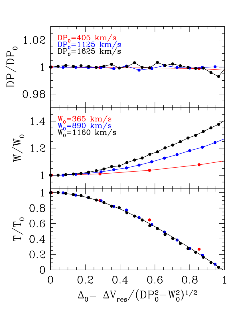
Figure 12: Impact of instrumental resolution on double-peaked profile parameters. The three panels show the evolution of $DP$, $W$ and $T$ versus the scaled-resolution parameter $\Delta_{0}$. $DP$, $W$ and $T$ are obtained by performing plain 2-Gaussian model fits to progressively degraded versions of synthetic double-peaked profiles that simulate the cases of Cen X-4 (red), A0620 (blue) and J1118 (black). The line profile parameters are plotted normalized to the initial (non-degraded) values $DP_{0}$, $W_{0}$ and $T_{0}$. The curved line in the bottom panel represents a cubic fit to the ensemble of points.

Fig. 12 depicts the evolution of the fitted parameters $DP$, $W$ and $T$ as a function of the scaled-resolution $\Delta_{0}$ for the three cases investigated. The parameters are shown normalized to their original non-degraded values. Interestingly, we observe that $DP$ is little affected by instrument resolution since it is measured to within $\sim$0.5 per cent of its initial value, even at poor resolutions (i.e. large $\Delta_{0}$ values). $W$, on the other hand, rises with $\Delta_{0}$ and, consequently, $T$ declines. In the limit when $\Delta V_{\rm res}=\sqrt{DP_{0}^{2}-W_{0}^{2}}$ (i.e. $\Delta_{0}=1$) the double peak trough vanishes since $T=0$. We find that the evolution of $T$ with instrumental resolution is well described by the cubic expression $T/T_{0}=1+(0.53\Delta_{0}-1.54)\Delta_{0}^{2}$.

Of course, when dealing with real data the intrinsic line parameters $DP_{0}$ and $W_{0}$ (and thus $\Delta_{0}$) are not known beforehand. In principle, these can be inferred by fitting 2-Gaussian models that are previously degraded to the resolution of the data (i.e. by convolution with a Gaussian of $FWHM=\Delta V_{\rm res}$) and this is the approach that we have followed throughout the paper. In order to test how close the inferred $DP$ and $W$ values are to the intrinsic quantities we have performed a simulation using real data. We have taken the average spectra of Cen X-4 plus the GTC spectra of A0620 and J1118 (see Section 3), and degraded them further through convolution with Gaussian functions of increasing widths. The effective resolution of the new degraded profiles will thus be the quadratic sum of the instrument resolution (i.e. 7, 140 and 120  km s^-1 for Cen X-4, A0620 and J1118, respectively) and the Gaussian convolution widths. We then performed 2-Gaussian model fits, degraded by their corresponding effective resolutions, to the new profiles. The results are plotted as a function of the scaled-resolution parameter in Fig. 13. Note that here we plot $\Delta=\Delta V_{\rm res}/\sqrt{DP^{2}-W^{2}}$ in the x-axis, where $DP$ and $W$ represent the inferred $DP_{0}$ and $W_{0}$ values, as derived from the fits. Since the initial instrumental resolution in the three binaries is sufficiently small we take the $DP$, $W$ and $T$ values measured from the original (non-degraded) profiles as the true unbiased quantities i.e. $DP_{0}$, $W_{0}$ and $T_{0}$.

The bottom panel of Fig. 13 shows that the $T$ values provided by the resolution-degraded model fits are still underestimated, but to a much lesser extent than before. In order to quantify the systematic shift in $T$ measurements we have fitted a quadratic function to the bottom panel of Fig. 13 and find

$$T-T_{0}=-0.097\Delta^{2}.$$ (10)

We observe that for $\Delta\leq 0.2$ (i.e. the case of our seven calibrators) the original $T$ values are accurately recovered to better than 0.005. As the scaled-resolution parameter increases, though, the measured $T$ values become more and more biased low. Still, for $\Delta<0.5$ the $T$ values are underestimated by less than the typical variability observed in multi-epoch observations (i.e. $\sigma(T)\simeq 0.025$) and, therefore, we conclude they are not significantly biased by instrumental resolution. Anyhow eq. 10 provides a way to correct for the systematic shift in $T$ measurements from resolution-degraded models that we believe is reliable up to $\Delta\approx 0.8$. For example, in the cases of J1357 and J0422, with $\Delta=0.42$ and 0.69, we estimate a correction of +0.017 and +0.046, respectively (Sect. 7).

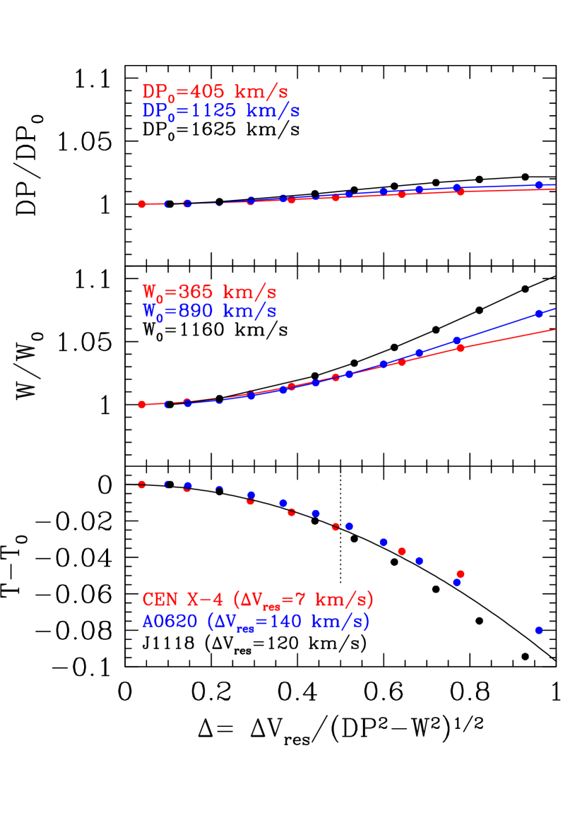
Figure 13: Deviation between the original line parameters ($DP_{0}$, $W_{0}$ and $T_{0}$) and those inferred by fitting resolution-degraded 2 Gaussian models. This simulation employs real Cen X-4, J1118 and A0620 spectra, progressively degraded with increasing resolutions. The curved solid line in the bottom panel represents a quadratic fit to the ensemble of points (eq. 10). The vertical dotted line marks a reference limit above which instrumental resolution starts to have a significant impact on $T$ values extracted from degraded models. In other words, for $\Delta>0.5$ the measured $T$ values are underestimated by more than the typical variability $\sigma(T)\approx 0.025$ observed in multi-epoch observations.

Appendix B Orbital dependence of line trough

The measurement of the line trough $T$ is best performed over orbital averages because (1) individual spectra rarely possess enough signal-to-noise for the fitting technique to be applicable and (2) orbital means average out possible asymmetries in individual spectra from, for example, hot-spots or disc eccentricities which could potentially bias the determination of $T$. We here explore the impact of limited phase coverage in $T$ measurements by fitting our 2-Gaussian model to a sample of systems with high quality phase-resolved individual spectra. These are the GTC spectra of J0422 (Section 7), A0620, J1118 and J1357, plus a VLT database on J1357 from Torres et al. (2015). The results are presented in Fig. 13.

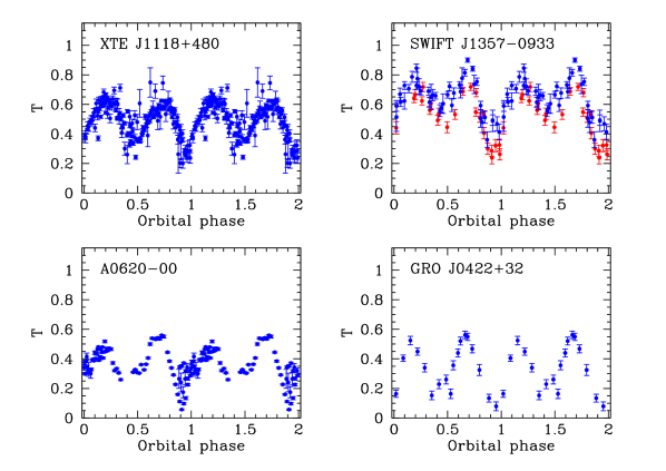
Figure 14: Orbital modulation of $T$ in a sample of BH XRTs. Red and blue points in the upper right panel represents two different data sets: 2013 VLT data from Torres et al. (2015) and 2014 GTC data from Mata Sánchez et al. (2015), respectively. The J1118 and A0620 data have been folded using ephemeris from González Hernández et al. (2014), while the J0422 data using those from Webb et al. (2000). In the case of J1357 we have used our new period determination $P_{\rm orb}=0.106969$ d and a tentative time of inferior conjunction of the companion star of HJD 2456396.6617, obtained by imposing that the deepest minimum is centered at phase 0.95.

All systems display a clear double-hump modulation of $T$ versus orbital phase, with maxima at phases 0.2 and 0.7 and minima at 0.45 and 0.95. The phasing suggests that the minima are caused by the crossing of S-waves (i.e. narrow emission-line components associated to the hot spot and the companion star) through the center of the line profile and this is confirmed by trailed spectrogram plots (see e.g. Marsh et al. 1994; Zurita et al. 2016). A sine fit with the period fixed to $0.5\times P_{\rm orb}$ yields a characteristic amplitude $\Delta T=\pm 0.15$. Given the double-sine shape of the modulation, $T$ values obtained from average spectra with $\gtrsim$ 50 per cent phase coverage must be close to the orbital mean and, therefore, not significantly biased.

On the other hand, we observe that the phase 0.95 minimum appears deeper than the minimum at phase 0.45. This can be explained by opacity effects since the hot-spot becomes obscured by the outer disc rim around phase 0.4 thus making the filling-in of the double peak trough less pronounced. As a matter of fact, the different minima can be exploited to determine the orbital period in systems where the companion star is totally veiled by the accretion disc. For example, we have performed a period analysis of the time evolution of $T$ in J1357. Fig. 14 presents the resulting Lomb-Scargle periodogram. The frequency of the highest peak corresponds to a period of 0.005348455$\pm$0.0000115 d, where the error is taken as the sigma of a Gaussian fit to the peak. Because of the double-humped shape of the $T$ curve we adopt twice this value as the true orbital period i.e. $P_{\rm orb}=0.106969\pm 0.000023$ d. This is consistent but much more precise than previous reports in Corral-Santana et al. (2013) and Mata Sánchez et al. (2015) because of the 14 months elapsed between the VLT and GTC observations. It should be noted that only the peak with the highest power produces a phase folded $T$ curve with unequal minima (see Fig. 13). This confirms that the next high peaks are caused by aliasing and can be discarded.

Figure 15: Lomb-Scargle periodogram of $T$ measurements from the 2013 VLT and 2014 GTC campaigns of J1357. The highest peak corresponds to our selected 0.106969 d period.

Appendix C Inclination reports disregarded from the calibration sample

In the particular case of A0620 we have dismissed the works of Shahbaz et al. (1994) ($i=31-54^{\circ}$) and Gelino et al. (2001a) ($i=41\pm 3^{\circ}$) because disc contamination is neglected (although the latter attempt to account for light curve asymmetries using a dark spot stellar model). Froning & Robinson (2001), on the other hand, do not provide a useful constrain to the disc contribution on their H-band light curves since the very wide range quoted ($i=38-75^{\circ}$) is virtually uninformative. Finally, we regard the result of Haswell et al. (1993) ($i=62-74^{\circ}$) as dubious as it relies on the identification of a tentative grazing eclipse that was never confirmed in subsequent higher quality light curves. We believe that a transient sharp asymmetry, associated for example to a running superhump wave (see an example in Zurita et al. 2002) provides a more plausible explanation to the data. Note that, despite Haswell’s data expand over several nights the authors applied a weighted process to produce their phased light curves because "the quality of the data varied significantly from night to night" (sic) so it seems possible that a sharp asymmetry on a high-quality night may stand up in the mean light curve.

Regarding N Mus 91, we have dismissed the work of Shahbaz et al. (1997) because the accretion disc contribution is neglected. Besides, the limited data quality results in a poorly constrained inclination value $i=39-64^{\circ}$. Likewise, we dismiss Orosz & Bailyn (1996) ($i=54-65^{\circ}$) and Gelino et al. (2001b) ($i=54\pm 2^{\circ}$) because the contamination by non-stellar sources is crudely modeled or neglected. These results are superseded by a later paper of the same group (Wu et al., 2016), that also incorporates a more extended photometric database from subsequent epochs. Wu et al. apply a careful filtering, selecting only light curves during passive state. In particular, a re-analisis of the light curves of Orosz & Bailyn (1996) and Gelino et al. (2001b) is performed, after correcting for accretion disc contamination and including a hot-spot contribution. They consistently find $i=43^{\circ}$ in all cases. In view of all this we decide to choose the result of Wu et al. (2016) as the best estimate available for the inclination in N Mus 91.

In the case of GS2000 we do not consider the work of Beekman et al. (1996) ($i=43-69^{\circ}$) because the accretion disc contribution is neglected when fitting ellipsoidal models to a limited quality H-band light curve.

As for J1118 we systematically ignore inclination measurements obtained when the system was in the decay phase. These are: McClintock et al. (2001) ($i\geq 55^{\circ}$), Wagner et al. (2001) ($i=81\pm 2^{\circ}$) and Zurita et al. (2002) ($i=71-82^{\circ}$).

Regarding J1550 we did not consider the work of Orosz et al. (2002) ($i=67-74^{\circ}$) because it is superseded by our selected paper Orosz et al. (2011) ($i=74.7\pm 3.8^{\circ}$). The latter work presents fits to new higher quality NIR light curves, together with a re-analysis of the older light curves from Orosz et al. (2002), including accretion disc contamination.

Finally, in the case of Cen X-4, we have dismissed Shahbaz et al. (1993) ($i=31-54^{\circ}$) because the accretion disc contribution is ignored. This work is superseded by Khargharia et al. (2010), one of our selected results, where the accretion disc contribution is estimated by means of NIR spectroscopy.

References

- Abbott et al. (2020a) Abbott B.P., 2020a, ApJ, 892, L3
- Abbott et al. (2020b) Abbott R., 2020b, ApJ, 896, L44
- Abbott et al. (2021) Abbott R., 2021, ApJ, in press, arXiv:2111.03606
- Armas Padilla et al. (2014) Armas Padilla M., Wijnands R., Altamirano D., Méndez M., Miller J.M., Degenaar N., 2014, MNRAS, 439, 3908
- Armitage et al. (1996) Armitage P.J., Livio M., Pringle J.E., 1996, ApJ, 457, 332
- Bailyn et al. (1998) Bailyn C.D., Jain R.K., Coppi P., Orosz J.A., 1998, ApJ, 499, 367
- Beekman et al. (1996) Beekman G., Shahbaz T., Naylor T., Charles P.A., 1996, MNRAS, 281, L1
- Beekman et al. (1997) Beekman G., Shahbaz T., Naylor T., Charles P.A., Wagner R.M., Martini P., 1997, MNRAS, 290, 303
- Belczynski et al. (2012) Belczynski K., Wiktorowicz G., Fryer C.L., Holz D.E., Kalogera V., 2012, ApJ, 757, 91
- Belloni et al. (2011) Belloni T.M., Motta S.E., Muñoz-Darias T., 2011, Bull. Astr. Soc. India, 39, 409
- Beri et al. (2019) Beri A., 2019, MNRAS, 485, 3064
- Callanan et al. (1996a) Callanan P.J., Garcia M.R., McClintock J.E., Zhao P., Remillard R.A., Haberl F., 1996a, ApJ, 461, 351
- Callanan et al. (1996b) Callanan P.J., Garcia M.R., Filippenko A.V., McLean I., Teplitz H., 1996b, ApJ, 470, L57
- Cantrell et al. (2010) Cantrell A.G. et al., 2010, ApJ, 710, 1127
- Casares (2015) Casares J., 2015, ApJ, 808, 80
- Casares (2016) Casares J., 2016, ApJ, 822, 99
- Casares (2018) Casares J., 2018, MNRAS, 473, 5195
- Casares et al. (1995a) Casares J., Charles P.A., Marsh T.R., 1995, MNRAS, 277, L45
- Casares et al. (1995b) Casares J., Martin A.C., Charles P.A., Martin E.L., Rebolo R., Harlaftis E.T., Castro-Tirado A. J., 1995b, MNRAS, 276, L35
- Casares et al. (1997) Casares J., Martín E.L., Charles P.A., Molaro P., Rebolo R., 1997, NewA, 1, 299
- Casares et al. (2007) Casares J., Bonifacio P., González Hernández J.I., Molaro P., Zoccali M., 2007, A&A, 470, 1033
- Casares & Jonker (2014) Casares J., Jonker P.G., 2014, Space Sci. Rev., 183, 223
- Casares et al. (2014) Casares J., Negueruela, I., Ribó, M., Ribas I., Paredes J.M., Herrero A., Simón-Díaz S., 2014, Nature, 505, 378
- Casares & Torres (2018) Casares J., Torres M.A.P., 2018, MNRAS, 481, 4372
- Chen et al. (2020) Chen A., Johnson-McDaniel N.K., Dietrich T., Dudi R., 2020, Phys. Rev. D, 101, 103008
- Cherepashchuk et al. (2019) Cherepashchuk A.M., Katysheva N.A., Khruzina T.S., 2019, MNRAS, 490, 32
- Copperwheat et al. (2010) Copperwheat C.M., Marsh T.R., Dhillon V.S., Littlefair S.P., Hickman R., Gänsicke, B.T., Southworth J., 2010, MNRAS, 402, 1824
- Copperwheat et al. (2012) Copperwheat C.M. et al., 2012, MNRAS, 421, 149
- Corral-Santana et al. (2013) Corral-Santana J.M., Casares J., Muñoz-Darias T., Rodríguez-Gil P., Shahbaz T., Torres M.A.P., Zurita C., Tyndall A.A., 2013, Science, 339, 1048
- Corral-Santana et al. (2016) Corral-Santana J.M., Casares J., Muñoz-Darias T., Bauer F.E., Martínez-Pais I.G., Russell D.M., 2016, A&A, 587, A61
- D’Avanzo et al. (2005) D’Avanzo P., Campana S., Casares J., Israel G.L., Covino S., Charles P.A., Stella L., 2005, A&A, 444, 905
- D’Avanzo et al. (2006) D’Avanzo P., Muñoz-Darias T., Casares J., Martínez-Pais I.G., Campana S., 2006, A&A, 460, 257
- Dermer & Atoyan (2006) Dermer C.D., Atoyan A., 2006, ApJ, 643, L13
- Echevarría et al. (2007) Echevarría J, de la Fuente E., Costero R., 2007, AJ, 104, 262
- El-Badry et al. (2022) El-Badry K., Seeburger R., Jayasinghe T., Rix H.-W., Almada S., Conroy C., Price-Whelan A.M., Burdge K., 2020, MNRAS, 512, 5620
- Ertl et al. (2020) Ertl T., Woosley S.E., Sukhbold T., Janka H.-T., 2020, ApJ, 890, 51
- Farr et al. (2011) Farr W.M., Niharika S., Cantrell A., Kreidberg. L., Bailyn C.D., Mandel I., Kalogera V., 2011, ApJ, 741, 103
- Filippenko et al. (1995) Filippenko A.V., Matheson T., Barth A.J., 1995, ApJ, 455, L139
- Foley et al. (2020) Foley R.J., Coulter D.A., Kilpatrick C.D., Piro A.L., Ramirez-Ruiz E., Schwab J., 2020, MNRAS, 494, 190
- Froning & Robinson (2001) Froning C.S., Robinson E.L., 2001, AJ, 121, 2212
- Frank, King & Raine (2002) Frank J., King A.R., Raine D.J., 2002, Accretion Power in Astrophysics, 3rd edn., Cambridge University Press
- Fryer & Kalogera (2001) Fryer C.L., Kalogera V., 2001, ApJ, 554, 548
- Gao et al. (2022) Gao S.-J., Li X.-D., Shao Y., 2022, MNRAS, 514, 1054
- Gelino et al. (2001a) Gelino D.M., Harrison T.E., Orosz J.A., 2001a, AJ, 122, 2668
- Gelino et al. (2001b) Gelino D.M., Harrison T.E., McNamara B.J., 2001b, AJ, 122, 971
- Gelino & Harrison (2003) Gelino D.M., Harrison T.E., 2003, ApJ, 599, 1254
- Gelino et al. (2006) Gelino D.M., Balman Ş., Kiziloğlu Ü., Yilmaz A., Kalemci E., Tomsick J.A., 2006, ApJ, 642, 438
- González Hernández et al. (2006) González Hernández J.I., Rebolo R., Israelian G., Harlaftis E.T., Filippenko A.V., Chornock R., 2006, ApJ, 644, L49
- González Hernández et al. (2008) González Hernández J.I., Rebolo R., Israelian G., Filippenko A.V., Chornock R., Tominaga N., Umeda H., Nomoto K., 2008, ApJ, 679, 732
- González Hernández et al. (2012) González Hernández J.I., Rebolo R., Casares J., 2012, ApJ, 744, L25
- González Hernández, Rebolo & Casares (2014) González Hernández J.I., Rebolo R., Casares J., 2014, MNRAS, 438, L21
- González Hernández et al. (2017) González Hernández J.I., Suárez-Andrés L., Rebolo R., Casares J., 2017, MNRAS, 465, L15
- Hammerstein et al. (2018) Hammerstein E.K., Cackett E.M., Reynolds M.T., Miller J.M., 2018, MNRAS, 478, 4317
- Han et al. (2020) Han M.-Z., Tang S.P., Hu Y.-M., Li Y.J., Jiang J.-L., Jin Z.-P., Fan Y.-Z., Wei D.-M., 2020, ApJ, 891, L5
- Harlaftis et al. (1999) Harlaftis E.T., Colier S., Horne K., Filippenko A.V., 1999, A&A, 341, 491
- Harlaftis et al. (1994) Harlaftis E.T., Marsh T.R., Dhillon V.S., Charles P.A., 1994, MNRAS, 267, 473
- Haswell et al. (1993) Haswell C.A., Robinson E.L., Horne K., Stiening R.F., Abbott T.M.C., 1993, ApJ, 411, 802
- Horne & Marsh (1986) Horne K., Marsh T.R., 1986, MNRAS, 218, 761
- Horne & Saar (1991) Horne K., Saar S.H.,1991, ApJ, 374, L55
- Horne, Wood & Stiening (1991) Horne K., Wood J.H., Stiening R.F.,1991, ApJ, 378, 271
- Hynes et al. (2002) Hynes R.I., Zurita C., Haswell C.A., Casares J., Charles P.A., Pavlenko E.P., Shugarov S.Yu., Lott D.A., 2002, MNRAS, 330, 1009
- Ioannou et al. (2004) Ioannou Z., Robinson E.L., Welsh W.F., Haswell C.A., 2004, AJ, 127, 481
- Jayasinghe et al. (2021) Jayasinghe T. et al. 2021, MNRAS, 504, 2577
- Johnston et al. (1989) Johnston H.M., Kulkarni S.R., Oke J.B., 1989, ApJ, 345, 492
- Khargharia et al. (2010) Khargharia J., Froning C.S., Robinson E.L., 2010, ApJ, 716, 1105
- Khargharia et al. (2013) Khargharia J., Froning C.S., Robinson E.L., Gelino D.M., 2013, AJ, 145, 21
- Kochanek (2014) Kochanek C.S., 2014, ApJ, 785, 28
- Kreidberg et al. (2012) Kreidberg L., Bailyn C.D., Farr W.M., Kalogera V., 2012, ApJ, 757, 36
- Kouveliotou et al. (1993) Kouveliotou C., Finger M.H., Fishman G.J., Meegan C.A., Wilson R.B., Paciesas W.S., Minamitani T., van Paradijs J., 1993, in AIP Conf. Proc. 280, Proc. Compton Gamma Ray Observatory, ed. M. Friedlan-der, N. Gehrels, & D. J. Macomb (New York : AIP), 319
- Littlefair et al. (2008) Littlefair S.P., Dhillon V.S., Marsh T.R., Gänsicke B.T., Southworth J., Baraffe I., Watson C.A., Copperwheat C., 2008, MNRAS, 388, 1582
- Marsh et al. (1994) Marsh T.R., Robinson E.L., Wood J.H., 1994, MNRAS, 266, 137
- Marsh & Dhillon (1997) Marsh T.R., Dhillon V.S., 1997, MNRAS, 292, 385
- Mata Sánchez et al. (2015) Mata Sánchez D., Muñoz-Darias T., Casares J., Corral-Santana J.M., Shahbaz T., 2015, MNRAS, 454, 2199
- Mata Sánchez et al. (2021) Mata Sánchez D., Rau, Álvarez Hernández A., van Grunsven T.F.J., Torres M.A.P., Jonker P.G., 2021, MNRAS, 506, 581
- Matthews et al. (2015) Matthews J.H., Knigge C., Long K.S., Sim S.A., Higginbottom N., 2015, MNRAS, 450, 3331
- McClintock et al. (2001) McClintock J.E., Garcia M.R., Caldwell N., Falco E.E., Garnavich P.M., Zhao P., 2001, ApJ, 551, L147
- McClintock & Remillard (2006) McClintock J.E., Remillard R.A., 2006, in Compact stellar X-ray sources, ed. W. Lewin & M. van der Klis, Cambridge Astrophysics Series No. 39, Cambridge University Press, p.157
- Miller-Jones et al. (2021) Miller-Jones J.C.A. et al., 2021, Science, 371, 1046
- Neilsen et al. (2008) Neilsen J., Steeghs D., Vrtilek V.D.., 2008, MNRAS, 384, 849
- Orosz et al. (1994) Orosz J.A., Bailyn C.D., Remillard R.A., McClintock J.E., Foltz C.B., 1994, ApJ, 436, 848
- Orosz & Bailyn (1995) Orosz J.A., Bailyn C.D., 1995, ApJ, 446, L59
- Orosz & Bailyn (1996) Orosz J.A., Bailyn C.D., McClintock J.E., Remillard R.A., 1996, ApJ, 468, 380
- Orosz et al. (2002) Orosz J.A. et al., 2002, ApJ, 568, 845
- Orosz et al. (2011) Orosz J.A., Steiner J.F., McClintock J.E., Torres M.A.P., Remillard R.A., Bailyn C.D., Miller J.M., 2011, ApJ, 730, 75
- Özel et al. (2010) Özel, F., Psaltis D., Narayan R., McClintock J.E., 2010, ApJ, 725, 1918
- Reid et al. (2014) Reid M.J., McClintock J.E., Steiner J.F., Steeghs D., Remillard R.A., Dhawan V., Narayan R., 2014, ApJ, 796, 2
- Reynolds et al. (2007) Reynolds M.T., Callanan P.J., Filippenko A.V., 2007, MNRAS, 374, 657
- Roques et al. (1994) Roques J.P. et al., 1994, ApJS, 92, 451
- Savoury et al. (2012) Savoury C.D.J., Littlefair S.P., Marsh T.R., Dhillon V.S., Parsons S.G., Copperwheat C.M., Steeghs D., 2012, MNRAS, 422, 469
- Shahbaz et al. (1993) Shahbaz T., Naylor T., Charles P.A., 1993, MNRAS, 265, 655
- Shahbaz et al. (1994) Shahbaz T., Naylor T., Charles P.A., 1994, MNRAS, 268, 765
- Shahbaz et al. (1997) Shahbaz T., Naylor T., Charles P.A., 1997, MNRAS, 285, 607
- Shahbaz et al. (2013) Shahbaz T., Russell D.M., Zurita C., Casares J., Corral-Santana J.M., Dhillon V.S., Marsh T.R., 2013, MNRAS, 434, 2696
- Shahbaz et al. (2014) Shahbaz T., Watson C.A., Dhillon V.S., 2004, MNRAS, 440, 504
- Shaw et al. (2016) Shaw A.W., Charles P.A., Casares J., Hernández Santisteban J.V., 2016, MNRAS, 463, 1314
- Skidmore et al. (2000) Skidmore W., Mason E., Howell S.B., Ciardi D.R., Littlefair S., Dhillon V.S., 2002, MNRAS, 318, 429
- Skidmore et al. (2002) Skidmore W., Wynn G.A., Leach R., Jameson R.F., 2002, MNRAS, 336, 12
- Smak (1981) Smak J., 1981, Acta Astron., 31, 395
- Southworth et al. (2006) Southworth J. et al., 2006, MNRAS, 373, 687
- Stover (1981) Stover R.J., 1981, ApJ, 248, 684
- Sunyaev et al. (1993) Sunyaev R.A., 1993, A&A, 280, L1
- Thompson et al. (2019) Thompson T.A. et al., 2019, Science, 366, 637
- Torres et al. (2002) Torres M.A.P., Casares J., Martínez-Pais I.G., Charles P.A., 2002, MNRAS, 334, 233
- Torres et al. (2015) Torres M.A.P., Jonker P.G., Miller-Jones J.C.A., Steeghs D., Repetto S., Wu J., 2015, MNRAS, 450, 4292
- Torres et al. (2021) Torres M.A.P., Jonker P.G., Casares J., Miller-Jones J.C.A., Steeghs D., 2021, MNRAS, 501, 2174
- Tulloch et al. (2009) Tulloch S.M., Rodríguez-Gil P., Dhillon V.S., 2009, MNRAS, 397, L82
- Ugliano et al. (2012) Ugliano M., Janka H.-T., Marek A., Arcones A., 2012, ApJ, 757, 69
- van den Heuvel & Tauris (2020) van den Heuvel E.P.J., Tauris T.M., 2020, Science, 368, 3282
- van der Hooft et al. (1999) van der Hooft F., 1999, ApJ, 513, 477
- van Dijk et al. (1995) van Dijk R., 1995, A&A, 296, L33
- van Grunsven et al. (2017) van Grunsven T.F.J., Jonker P.G., Verbunt F.W.M., Robinson E.L., 2017, MNRAS, 472, 1907
- van Spaandonk et al. (2010) van Spaandonk L., Steeghs D., Marsh T.R., Torres M.A.P., 2010, MNRAS, 401, 1857
- Vietri & Stella (1999) Vietri M., Stella L., 1999, ApJ, 527, L43
- Vikhlinin et al. (1995) Vikhlinin A. et al., 1995, ApJ, 441, 779
- Wade & Horne (1988) Wade R.A., Horne K., 1988, MNRAS, 324, 411
- Wagner et al. (2001) Wagner R.M., Foltz C.B., Shahbaz T., Casares J., Charles P.A., Starrfield S.G., Hewett P., 2001, ApJ, 556, 42
- Webb et al. (2000) Webb N.A., Naylor T., Ioannou Z., Charles P.A., Shahbaz T., 2000, MNRAS, 317, 528
- Woosley et al. (2020) Woosley S.E., Sukhbold T., Janka H.-T., 2020, ApJ, arXiv:2020.10492
- Wu et al. (2015) Wu J. et al., 2015, ApJ, 806, 92
- Wu et al. (2016) Wu J., Orosz, J.A., McClintock J.E., Hasan I., Bailyn C.D., Gou L., Chen Z., 2016, ApJ, 825, 46
- Wyrzykowski & Mandel (2020) Wyrzykowski L., Mandel I., 2020, A&A, 636, 20
- Zhang & Robinson (1987) Zhang E.-H., Robinson E.L., 1987, ApJ, 321, 813
- Zurita et al. (2002) Zurita C. et al., 2002, MNRAS, 333, 791
- Zurita et al. (2003) Zurita C., Casares J., Shahbaz T., 2003, ApJ, 582, 369
- Zurita et al. (2015) Zurita C., Corral-Santana J.M., Casares J., 2015, MNRAS, 454, 3351
- Zurita et al. (2016) Zurita C., González Hernández J.I., Escorza A., Casares J., 2016, MNRAS, 460, 4289