Breaking Feedback Loops in Recommender Systems with Causal Inference

Abstract

Recommender systems play a key role in shaping modern web ecosystems. These systems alternate between (1) making recommendations (2) collecting user responses to these recommendations, and (3) retraining the recommendation algorithm based on this feedback. During this process, the recommender influences the user behavioral data that is subsequently used to update the recommender itself, thus creating a feedback loop. Recent work has shown that feedback loops may compromise recommendation quality and homogenize user behavior, raising ethical and performance concerns around deploying recommender systems. To address these concerns, we propose the causal adjustment for feedback loops (cafl), an algorithm that uses causal inference to break feedback loops for any loss-minimizing recommendation algorithms. The key observation is that a recommender system does not suffer from feedback loops if it reasons about causal quantities, namely the intervention distributions of recommendations on user ratings. Moreover, we can calculate these intervention distributions from observational data by adjusting for the recommender system’s predictions of user preferences. Using simulated environments, we demonstrate that cafl improves recommendation quality when compared to prior correction methods.

1 Introduction

Recommender systems are deployed in dynamic environments. At each time step, a recommender system makes recommendations and collects user feedback. At the next time step, the recommendation algorithm is updated based on this feedback. The process alternates between these two steps, inducing a feedback loop: the recommendation algorithm influences what user behavior data it observes; this data in turn affects the recommendation algorithm, since the algorithm is trained on this data. Over time, the issue is exacerbated: the recommender system is trained on a growing set of data points that have been biased by recommendations.

Uncontrolled feedback loops create negative externalities that are shouldered by consumers and producers. For example, they compromise recommendation quality as they bias the behavioral data collected by the system. They also exacerbate homogenization effects (Chaney et al., 2018): if a user interacts with an item early on, the recommendation system is more likely to recommend similar items at the expense of dissimilar items that the user might prefer. A related issue is the “rich-get-richer” problem where items that are popular early on are undeservedly recommended over newer items since the recommender system has observed more data about them (Chakrabarti et al., 2006; Salganik et al., 2006).

A naive way to break feedback loops is to recommend random items. Such a system does not suffer from negative feedback effects because its recommendations no longer depend on past data, but it does not learn from user behavior and would unacceptably degrade recommendation quality. So how can we break feedback loops without making recommendations useless?

In this work, we study the causal mechanism underlying the recommendation process and propose the causal adjustment for feedback loops (cafl), an algorithm that can provably break feedback loops in recommender systems. Studying feedback loops with a causal lens leads to a key observation: recommendation algorithms do not suffer from feedback loops if they reason about causal quantities, namely the intervention distributions of recommendations on user ratings. The reason is that a do intervention on a causal graph, by definition, breaks the connection between the variable being intervened on (e.g., the recommendation) and its normal causes (e.g., user feedback) (Pearl, 2009).

The causal mechanism of recommendation also reveals that the intervention distributions of recommendations are identifiable from observational data. To calculate the intervention distributions, it is sufficient to adjust for the recommender system’s predictions, since feedback loops in recommender systems only occur through this quantity (see Fig. 1(b)). Following this observation, we show how to design an algorithm, cafl, that estimates intervention distributions in training any loss-minimizing recommendation algorithms. cafl enables recommender systems to break feedback loops without resorting to random recommendations. In particular, it can be applied to situations where common causal assumptions (e.g. positivity (Imbens and Rubin, 2015)) are violated. For example, cafl can be applied when a recommender system requires that all items can only be recommended at most once to each user, which violates the positivity conditions required by standard causal adjustment methods (e.g. backdoor adjustment or inverse propensity weighting).

Contributions.  The contributions of this work are three-fold. (1) We formalize the operation of recommender systems over time as a structural causal model over multiple time steps. (2) We introduce cafl: a causal adjustment algorithm that can provably break feedback loops for existing recommendation algorithms. cafl is easy to implement in existing recommender systems as it only requires changing the weights of their loss function. (3) Across multiple simulation environments, we show that cafl not only corrects the dataset bias caused by feedback loops, but also improves predictive performance, moreso than prior correction methods. cafl can also reduce homogenization when feedback loops induce recommendation homogenization.

Related work.  This work is motivated by a recent line of research that aims to understand the effect of feedback loops in recommender systems. Using simulations, Schmit and Riquelme (2018) and Krauth et al. (2020) have shown that ignoring feedback effects will negatively impact performance. As recommender systems observe more data, they are also prone to homogenization and bias amplification, which researchers often attribute to feedback effects (Chaney et al., 2018; Mansoury et al., 2020). Another related line of work studies the effects of feedback loops theoretically: under assumptions of preference drifts, they show that feedback loops can have undesirable effects on users (Jiang et al., 2019; Kalimeris et al., 2021). Sharma et al. (2015); Hosseinmardi et al. (2020) further illustrate the impacts of recommender systems and feedback loops using observational data from large internet platforms.

Feedback loops can induce a sampling bias in the collected user behavior dataset, so the feedback loop problem is a form of the missing-not-at-random (mnar) problem over multiple time steps (Marlin and Zemel, 2009). The mnar problem has been extensively studied in single-step recommender systems: the recommender system aims to infer missing ratings over a single timestep using a static dataset. One approach to this problem is to assume an exposure model between users and items and corrects the bias such an exposure model would induce (Sinha et al., 2016; Hernández-Lobato et al., 2014; Liang et al., 2016). Another approach is to use tools from causal inference to correct this bias under different assumptions (Schnabel et al., 2016; Bonner and Vasile, 2018; Wang et al., 2020). In contrast to these works that focus on single-step recommender systems, this work studies the setting over multiple time steps and proposes adjustments based on the special structure of feedback loops.

Correcting feedback effects in recommender system is comparatively less studied than the mnar problem. Earlier work augments algorithms with temporal information, but does not model feedback effects (Koren, 2009). More recently, Sun et al. (2019) combines inverse propensity weighting (IPW) with active learning to correct for feedback effects, assuming the same rating model as Liang et al. (2016). Pan et al. (2021) modify their IPW correction to account for sequential effects. However, their method requires the marginal probability of an item being observed at each time step. Estimating these probabilities requires access to observational user data over a long period of time; the algorithm is thus unable to correct for feedback effects at the initial period when estimation is performed. Further, estimating these marginal probabilities is a challenging task, which compromises the prediction accuracy of algorithms even at later time steps. In contrast to these works, the cafl algorithm only requires calculating the probabilities of an item being recommended conditioned on the history of observed data, which is available to the recommender system. As a result, cafl is data-efficient, simple, and does not require strong modeling assumptions.

Finally, the problem of feedback loops in training machine learning algorithms is not unique to recommender systems. Farquhar et al. (2021) focus on the problem of active learning where one collect one data point at each time step; they propose two unbiased weighting estimators for empirical risk minimization. Perdomo et al. (2020) present a general framework to study the impact of feedback loops in machine learning predictions. In contrast to these works, the cafl algorithm takes an explicitly causal view of the feedback loop. It leads to unbiased weighting estimators that are applicable to recommender systems with multiple data points acquired in a single time step. The explicit causal view also enables the use of other causal adjustment strategies for breaking feedback loops, e.g., backdoor adjustment.

(a)

(b)

Figure 1: (a) Feedback loops depict the process where the recommendations $\mathbf{\boldsymbol{A}}$ affect the ratings $\mathbf{\boldsymbol{R}}$. They in turn affect the recommendation $\mathbf{\boldsymbol{A}}$ because recommendation algorithms are trained on the collected ratings data. (b) The causal graph of recommender systems over multiple times steps with feedback loops unrolled.

2 Feedback loops in recommender systems

We describe feedback loops and their consequences in recommender systems. We focus on multi-step recommender systems; these systems are regularly retrained as they collect more data.

2.1 Multi-step recommender systems

A multi-step recommender system operates over $T$ time steps. At each time step, it makes recommendations to users, observes their feedback, and is then retrained on all the data observed so far.

A multi-step recommender system begins with a set of $U$ new users and $I$ new items. At time step $t=1$, it recommends $N$ items to a random set of users. Denote $\mathbf{\boldsymbol{A}}_{t}$ as the $U\times I$ recommendation matrix, where its $(u,i)$-entry $A_{t,ui}$ is a binary variable that indicates whether user $u$ was recommended item $i$ at time $t$. Then, at time $t=1$, we have $\mathbf{\boldsymbol{A}}_{1}\stackrel{{\scriptstyle iid}}{{\sim}}\mathrm{Multinomial}(n=N,p=\mathbf{p}_{0})$, where $\mathbf{p}_{0}$ is a matrix of the initial probabilities of recommendation each item to each user.

After making recommendations, the multi-step recommender then collects user ratings on the items consumed at this time step. We denote the data we collect at time $t$ as $\mathbf{\boldsymbol{R}}_{t}$, which is a $U\times I$ rating matrix; its $(u,i)$-entry $R_{t,ui}$ is user $u$’s rating of item $i$ if the item is consumed at time step $t$, and $R_{t,ui}=0$ otherwise.

Given the user ratings, the multi-step recommender then infers users’ preferences based on the collected data from this first time step, $\left\{\mathbf{\boldsymbol{A}}_{1},\mathbf{\boldsymbol{R}}_{1}\right\}$. Denote $\hat{\Theta}_{t}$ as the inferred user preference and item attribute parameters at time $t$, which are usually minimizers of some loss function. More formally, the inferred user preference $\hat{\Theta}_{t}$ can be seen as a maximum likelihood estimator under some parametric probability model $P_{\Theta}$ with parameter $\hat{\Theta}$,

$$\hat{\Theta}_{1} =\operatorname*{arg\,min}_{\Theta}\,\mathbb{E}_{\mathbf{\boldsymbol{A}}_{1}}\left[\mathbb{KL}\left(P\left(\mathbf{\boldsymbol{R}}_{1}\,|\,\mathbf{\boldsymbol{A}}_{1}\right)||P_{\Theta}\left(\mathbf{\boldsymbol{R}}_{1}\,|\,\mathbf{\boldsymbol{A}}_{1}\right)\right)\right]$$ (1)

$$=\operatorname*{arg\,max}_{\Theta}\mathbb{E}_{\mathbf{\boldsymbol{A}}_{1}}\left[\mathbb{E}_{P(\mathbf{\boldsymbol{R}}_{1}\,|\,\mathbf{\boldsymbol{A}}_{1})}\left[\log P_{\Theta}\left(\mathbf{\boldsymbol{R}}_{1}\,|\,\mathbf{\boldsymbol{A}}_{1}\right)\right]\right],$$ (2)

where $P\left(\mathbf{\boldsymbol{R}}_{1}\,|\,\mathbf{\boldsymbol{A}}_{1}\right)$ is the (population) conditional distribution of $\mathbf{\boldsymbol{R}}_{1}$ given $\mathbf{\boldsymbol{A}}_{1}$, from which the collected data $\left\{\mathbf{\boldsymbol{A}}_{1},\mathbf{\boldsymbol{R}}_{1}\right\}$ is drawn, and $P_{\Theta}\left(\mathbf{\boldsymbol{R}}_{1}\,|\,\mathbf{\boldsymbol{A}}_{1}\right)$ is a parametric model we posit. $\mathbb{KL}(\cdot||\cdot)$ denotes the Kullback–Leibler divergence between the two distributions.

Many existing recommendation algorithms fall into this setup. For example, assuming a probabilistic matrix factorization (prob-mf) model for ratings (Mnih and Salakhutdinov, 2008) is equivalent to fitting $\hat{\Theta}$ through a Gaussian linear factor model with maximum likelihood estimation, $P_{\Theta}\left(\mathbf{\boldsymbol{R}}_{1}\,|\,\mathbf{\boldsymbol{A}}_{1}\right)=\prod_{u=1}^{U}\prod_{i=1}^{I}\mathcal{N}\left(R_{1,ui}\,|\,\theta_{u}^{\top}\beta_{i}\cdot A_{1,ui},\sigma^{2}\right),$ where the $K\times 1$ user vectors $\theta_{u}$ and the $K\times 1$ item vectors $\beta_{i}$ constitute the parameters $\Theta=\left((\theta_{u})_{u=1}^{U},(\beta_{i})_{i=1}^{I}\right)$, and $\sigma^{2}$ is assumed known. Similarly, performing weighted matrix factorization (Hu et al., 2008) and nonnegative factorization (Gopalan et al., 2014, 2015) also correspond to fitting parametric probability models using maximum likelihood (Wang et al., 2020).

After fitting a parametric model of user preferences, the recommender system then recommends items based on the inferred user preferences; that is, $\mathbf{\boldsymbol{A}}_{2,u}{\sim}P_{u}(\mathbf{\boldsymbol{A}}_{2,u}\,|\,\hat{\Theta}_{1}),u=1,\ldots,U$, where $P_{u}(\mathbf{\boldsymbol{A}}_{2,u}=1\,|\,\hat{\Theta}_{1})$ describes the probability of each item being recommended to user $u$ based on the inferred parameters $\hat{\Theta}_{1}$. This distribution $P_{u}(\cdot\,|\,\hat{\Theta})$ captures how recommender systems make decisions based on user preferences; it is usually specified by recommender systems a priori and can target different goals. For example, a recommender system may set up $P_{u}(\cdot\,|\,\hat{\Theta})$ to maximize the potential rating of recommended items, or to increase user consumption, or to maximize the diversity of the recommendations without sacrificing users’ utility by more than 10%.

Going from time $t=1$ to time $t=2,\ldots,T$, a multi-step recommender system further updates its inferred preferences, unlike a one-step recommender system which does not update its inferred user preferences. At time $t$, it makes new recommendations $\mathbf{\boldsymbol{A}}_{t}$, collects new data $\left\{\mathbf{\boldsymbol{A}}_{t},\mathbf{\boldsymbol{R}}_{t}\right\}$, and updates its parameters $\hat{\Theta}_{t}$ by fitting the model to $P(\{\mathbf{\boldsymbol{R}}_{s}\}_{s=1}^{t}\,|\,\{\mathbf{\boldsymbol{A}}_{s}\}_{s=1}^{t})$ using all the data collected up to this point, $\left\{(\mathbf{\boldsymbol{A}}_{1},\mathbf{\boldsymbol{R}}_{1}),(\mathbf{\boldsymbol{A}}_{2},\mathbf{\boldsymbol{R}}_{2})\ldots,(\mathbf{\boldsymbol{A}}_{t},\mathbf{\boldsymbol{R}}_{t})\right\}.$

But how should a recommender system update its user preference parameters $\hat{\Theta}_{t}$ after the first time step? In particular, the data collected from different time steps are not independent. Future recommendations depend on past ratings because the recommender system tries to recommend items that users will like, which is inferred from past ratings. Handling this dependence over time is a core challenge in developing multi-step recommender systems since naively repeating the optimization problem in Equation 3 would be sub-optimal.

2.2 Feedback loops in recommender systems

To handle the dependence between data points collected at different time steps, we study their dependency structure. This dependency structure is often referred to as feedback loops in recommender systems, describing how $\left(\mathbf{\boldsymbol{A}}_{t},\mathbf{\boldsymbol{R}}_{t}\right)$—the data collected at time $t$—depends on the data collected at all previous time steps, $\left\{\left(\mathbf{\boldsymbol{A}}_{1},\mathbf{\boldsymbol{R}}_{1}\right),\ldots,\left(\mathbf{\boldsymbol{A}}_{t-1},\mathbf{\boldsymbol{R}}_{t-1}\right)\right\}$.

In more detail, feedback loops refer to the $\mathbf{\boldsymbol{A}}\rightarrow\mathbf{\boldsymbol{R}}\rightarrow\mathbf{\boldsymbol{A}}$ loop, going from the recommendation $\mathbf{\boldsymbol{A}}_{t}$, to the rating $\mathbf{\boldsymbol{R}}_{t}$, and finally back to the recommendation $\mathbf{\boldsymbol{A}}_{t+1}$ (Fig. 1(a)). The recommender system begins by making recommendations $\mathbf{\boldsymbol{A}}_{t}$, these recommendations increase the probability of the recommended items being rated, hence affecting the rating we observe $\mathbf{\boldsymbol{R}}_{t}$. The collected ratings $\mathbf{\boldsymbol{R}}_{t}$—together with all past collected ratings—in turn, affect the recommendation matrix $\mathbf{\boldsymbol{A}}_{t+1}$, because the recommender infers user preferences from this data and makes recommendations based on this inference.

To learn user preferences from this sequentially collected data, the most common approach is to aggregate the data from different time steps (Lee et al., 2016; Sedhain et al., 2015; Zheng et al., 2016; Wang et al., 2006; Rendle, 2012; Steck, 2019; Ning and Karypis, 2011). We fit the probability model for the first time step (i.e. Eq. 1) to all the data collected up to time $t$, and infer user preferences as follows:

$$\hat{\Theta}_{t}^{\mathrm{naive}} =\operatorname*{arg\,max}_{\Theta}\sum_{s=1}^{t}\mathbb{E}_{\mathbf{\boldsymbol{A}}_{s}}\left[\mathbb{E}_{P(\mathbf{\boldsymbol{R}}_{s}\,|\,\mathbf{\boldsymbol{A}}_{s})}\left[\log P_{\Theta}\left(\mathbf{\boldsymbol{R}}_{s}\,|\,\mathbf{\boldsymbol{A}}_{s}\right)\right]\right]$$ (3)

$$=\operatorname*{arg\,min}_{\Theta}\,\mathbb{E}\left[\mathbb{KL}\left(\prod_{s=1}^{t}P\left(\mathbf{\boldsymbol{R}}_{s}\,|\,\mathbf{\boldsymbol{A}}_{s}\right)||\prod_{s=1}^{t}P_{\Theta}\left(\mathbf{\boldsymbol{R}}_{s}\,|\,\mathbf{\boldsymbol{A}}_{s}\right)\right)\right].$$ (4)

This approach considers a product of the likelihood terms from each time step, implicitly assuming data $\{\mathbf{\boldsymbol{A}}_{t},\mathbf{\boldsymbol{R}}_{t}\}$ observed at different time steps are independently collected. However, they are in general not independent in multi-step recommender systems, that is,

$$P(\{\mathbf{\boldsymbol{R}}_{s}\}_{s=1}^{t}\,|\,\{\mathbf{\boldsymbol{A}}_{s}\}_{s=1}^{t})=\prod_{s=1}^{t}P(\mathbf{\boldsymbol{R}}_{s}\,|\,\mathbf{\boldsymbol{A}}_{s},\{\mathbf{\boldsymbol{R}}_{s^{\prime}},\mathbf{\boldsymbol{A}}_{s^{\prime}}\}_{s^{\prime}=1}^{s-1})\neq\prod_{s=1}^{t}P(\mathbf{\boldsymbol{R}}_{s}\,|\,\mathbf{\boldsymbol{A}}_{s})$$ (5)

since $P(\{\mathbf{\boldsymbol{A}}_{s},\mathbf{\boldsymbol{R}}_{s}\}_{s=1}^{t})\neq\prod_{s=1}^{t}P(\mathbf{\boldsymbol{R}}_{s},\mathbf{\boldsymbol{A}}_{s})$. The only exception is when all recommendations $\mathbf{\boldsymbol{A}}_{s}$’s are completely random, and thus they do not depend on past observations. By treating dependent data as if they were independent, $\hat{\Theta}_{t}^{\mathrm{naive}}$ is a biased estimator of user preferences.

Beyond biased estimation, feedback loops are also known to produce a “rich get richer” phenomenon, leading to homogenization in recommendations over time (Chaney et al., 2018). As an example, we contrast two toy movie recommender systems, one with feedback loops (making recommendations based on $\hat{\Theta}_{t}^{\mathrm{naive}}$ at time $t$) and one without feedback loops (making random recommendations at time $t$). We then consider their recommendations to two different users: user A likes both drama and horror movies, and user B likes both drama and sci-fi movies.

The recommender with feedback loops often experiences recommendation homogenization over time. For example, suppose it recommends drama movies to both users at $t=1$ by chance. Both users will rate it highly because the recommendation aligns with (part of) their preferences. The recommender then collects these ratings and infers that both users like drama movies. It thus continues to recommend drama movies at $t=2$, and again both users will rate it highly. Continuing with this process, the recommender with feedback loops will incorrectly infer that the two users have the same preferences, hence homogenizing user recommendations.

In contrast, the recommender without feedback loops does not homogenize recommendations. Again suppose it recommends a drama movie to both users at $t=1$ by chance; both users rate it highly; the recommender will then infer that both like drama movies, as with the recommender with feedback loops. At time $t=2$, however, the recommender will not solely recommend drama movies. Rather, it may recommend some other movies like a sci-fi movie. In this case, only user B may rate it highly. With this data from $t=2$, the recommender will correctly infer that the two users have different user preferences.

Given these concerns about biased and homogenized recommendations, multi-step recommender systems ought to avoid feedback loops (Chaney et al., 2018). One immediate way to avoid feedback loops is to adopt a random recommendation mechanism. Such recommendations are not affected by past ratings and thus are feedback-free. But the user experience will suffer with random recommendations. How can we then break the feedback loop without making random recommendations? In the next sections, we analyze the causal mechanism of feedback loops and show that a recommender system does not suffer from feedback loops if it reasons about causal quantities, namely the intervention distributions of recommendations $\mathbf{\boldsymbol{A}}_{s}$ on ratings $\mathbf{\boldsymbol{R}}_{s}$. This observation leads us to develop a causal adjustment algorithm that can provably break feedback loops without resorting to random recommendations.

3 Breaking Feedback Loops in Recommendation Systems with Causal Inference

We begin with a description of the causal mechanism of feedback loops in recommender systems. This causal perspective will lead to an adjustment algorithm that can provably break feedback loops.

3.1 The causal mechanism of feedback loops

To break feedback loops, we first study its causal mechanism by unrolling it over $t$ time steps.

Begin by writing down the causal graphical model (Pearl, 2009) of recommender systems in Fig. 1(b). At time $t=1$, the recommender system begins with some recommendations $\mathbf{\boldsymbol{A}}_{1}$. These recommendations causally affect the observed user ratings $\mathbf{\boldsymbol{R}}_{1}$ by increasing the probability of the recommended items being rated. Both the recommendations and the observed ratings also affect the inferred user preference parameters $\hat{\Theta}_{1}$ since the recommender optimizes $\hat{\Theta}_{1}$ based on $\left\{\mathbf{\boldsymbol{A}}_{1},\mathbf{\boldsymbol{R}}_{1}\right\}$. This inferred user preference $\hat{\Theta}_{1}$ then affects $\mathbf{\boldsymbol{A}}_{2}$, i.e. what items are recommended at $t=2$.

The causal structure of $\left\{\mathbf{\boldsymbol{A}}_{1},\mathbf{\boldsymbol{R}}_{1},\hat{\Theta}_{1},\mathbf{\boldsymbol{A}}_{2}\right\}$ then repeats itself at each time step $t$. In particular, the inferred user preferences $\hat{\Theta}_{t}$ generally depends on all past recommendations and ratings $\left\{\mathbf{\boldsymbol{A}}_{1:(t-1)},\mathbf{\boldsymbol{R}}_{1:(t-1)}\right\}$. Finally, the (unobserved) true user preferences $\Theta$ affects all ratings across all time steps, hence there is an arrow from $\Theta$ to all $\left(\mathbf{\boldsymbol{R}}_{t}\right)_{t=1}^{T}.$

The existence of feedback loops is evident in the causal graph (Fig. 1(b)), where past recommendations and ratings constantly inform future recommendations. The data $\left\{\mathbf{\boldsymbol{A}}_{t},\mathbf{\boldsymbol{R}}_{t}\right\}$ collected at different time steps are thus not independent, i.e. $P(\{\mathbf{\boldsymbol{R}}_{s}\}_{s=1}^{t}\,|\,\{\mathbf{\boldsymbol{A}}_{s}\}_{s=1}^{t})\neq\prod_{s=1}^{t}P(\mathbf{\boldsymbol{R}}_{s}\,|\,\mathbf{\boldsymbol{A}}_{s})$ as in Eq. 5; they causally depend on each other, preventing us from fitting a single model to the data from all time steps. Given the causal graph from Fig. 1(b), how can we break the feedback loop $\mathbf{\boldsymbol{A}}\rightarrow\mathbf{\boldsymbol{R}}\rightarrow\mathbf{\boldsymbol{A}}\rightarrow\mathbf{\boldsymbol{R}}\rightarrow\mathbf{\boldsymbol{A}}\rightarrow\cdots$ in updating recommendation algorithms and fitting $\hat{\Theta}_{t}$?

3.2 Breaking feedback loops in recommender systems using causal inference

To break the feedback loops in Fig. 1(b), we need to find a distribution $\tilde{P}$ about recommendations and ratings $\left\{\mathbf{\boldsymbol{A}}_{s},\mathbf{\boldsymbol{R}}_{s}\right\}_{s=1}^{t}$ such that it does achieve independence over time steps, i.e. $\tilde{P}(\{\mathbf{\boldsymbol{R}}_{s}\}_{s=1}^{t}\,|\,\{\mathbf{\boldsymbol{A}}_{s}\}_{s=1}^{t})=\prod_{s=1}^{t}\tilde{P}(\mathbf{\boldsymbol{R}}_{s}\,|\,\mathbf{\boldsymbol{A}}_{s})$. Such a distribution does not suffer from feedback loops or their resulting model-fitting bias in Eq. 3; it would allow us to learn user preference parameters $\hat{\Theta}_{t}$ from all past time steps.

Causal inference provides a solution to this challenge: the intervention distribution of recommendations on ratings $P(\mathbf{\boldsymbol{R}}_{s}\,|\,\mathrm{do}(\mathbf{\boldsymbol{A}}_{s}=\mathbf{\boldsymbol{a}}))$ achieves this independence and does not suffer from feedback loops (Pearl, 2009). In more detail, $P(\mathbf{\boldsymbol{R}}_{s}\,|\,\mathrm{do}(\mathbf{\boldsymbol{A}}_{s}=\mathbf{\boldsymbol{a}}))$ denotes the distribution of $\mathbf{\boldsymbol{R}}_{s}$ under the intervention of setting $\mathbf{\boldsymbol{A}}_{s}$ to be equal to the value $a$. It does not suffer from feedback loops because, by definition, a do intervention $\mathrm{do}(\mathbf{\boldsymbol{A}}_{s}=\mathbf{\boldsymbol{a}})$ breaks the connection between the variables being intervened on $\mathbf{\boldsymbol{A}}_{s}$ and its parents $\hat{\Theta}_{s-1}$ in the causal graph (Fig. 1(b)), thus breaking the $\mathbf{\boldsymbol{A}}_{s}\rightarrow\mathbf{\boldsymbol{R}}_{s}\rightarrow\mathbf{\boldsymbol{A}}_{s+1}$ feedback loop. The following lemma formalizes this argument.

Lemma 1.

Assuming the causal graph in Fig. 1(b), we have

$$P(\{\mathbf{\boldsymbol{R}}_{s}\}_{s=1}^{t}\,|\,\mathrm{do}(\{\mathbf{\boldsymbol{A}}_{s}\}_{s=1}^{t}=\{\mathbf{\boldsymbol{a}}_{s}\}_{s=1}^{t})=\prod_{s=1}^{t}P(\mathbf{\boldsymbol{R}}_{s}\,|\,\mathrm{do}(\mathbf{\boldsymbol{A}}_{s}=\mathbf{\boldsymbol{a}}_{s})),\\ \forall\mathbf{\boldsymbol{a}}_{s}\in\{0,1\}^{U\times I},t\in\{2,\ldots,T\}.$$ (6)

Lemma 1 is an immediate consequence of the do calculus (Pearl, 2009).

Moreover, the intervention distribution is the distribution with the highest fidelity to the observational data while staying immune from feedback loops. More precisely, among all distributions $\tilde{P}$ that satisfy independence across time steps (Eq. 6), the intervention distribution $\prod_{s=1}^{t}P(\mathbf{\boldsymbol{R}}_{s}\,|\,\mathrm{do}(\mathbf{\boldsymbol{A}}_{s}=\mathbf{\boldsymbol{a}}))$ is the distribution that is closest to $\tilde{P}\left(\{\mathbf{\boldsymbol{R}}_{s}\}_{s=1}^{t}\,|\,\{\mathbf{\boldsymbol{A}}_{s}\}_{s=1}^{t}\right)$ in Kullback-Leibler (kl) divergence:

Lemma 2.

Assuming the causal graph in Fig. 1(b), we have, for all $\mathbf{\boldsymbol{a}}_{s}\in\{0,1\}^{U\times I}$ and $t\in\{2,\ldots,T\}$,

$$\prod_{s=1}^{t}P(\mathbf{\boldsymbol{R}}_{s}\,|\,\mathrm{do}(\mathbf{\boldsymbol{A}}_{s}=\mathbf{\boldsymbol{a}}_{s}))$$

$$=\operatorname*{arg\,min}_{\tilde{P}\in\mathcal{Q}}\mathbb{KL}\left(P(\{\mathbf{\boldsymbol{R}}_{s}\}_{s=1}^{t}\,|\,\{\mathbf{\boldsymbol{A}}_{s}\}_{s=1}^{t}=\{\mathbf{\boldsymbol{a}}_{s}\}_{s=1}^{t})\Big{|}\Big{|}\tilde{P}(\{\mathbf{\boldsymbol{R}}_{s}\}_{s=1}^{t}\,|\,\{\mathbf{\boldsymbol{A}}_{s}\}_{s=1}^{t}=\{\mathbf{\boldsymbol{a}}_{s}\}_{s=1}^{t})\right),$$ (7)

where $\mathcal{Q}=\left\{\tilde{P}:\tilde{P}(\{\mathbf{\boldsymbol{R}}_{s}\}_{s=1}^{t}\,|\,\{\mathbf{\boldsymbol{A}}_{s}\}_{s=1}^{t}=\{\mathbf{\boldsymbol{a}}_{s}\}_{s=1}^{t})=\prod_{s=1}^{t}\tilde{P}(\mathbf{\boldsymbol{R}}_{s}\,|\,\mathbf{\boldsymbol{A}}_{s}=\mathbf{\boldsymbol{a}}_{s})\right\}$ is the set of all distributions that satisfies the independence relationship in Eq. 6.

Lemma 2 is an immediate consequence of Theorem 1 in Wang et al. (2019).

Taken together, Lemmas 1 and 2 imply that, to avoid feedback loops in recommender system, one should fit the parametric model $P_{\Theta}$ to the intervention distributions $P(\mathbf{\boldsymbol{R}}_{s}\,|\,\mathrm{do}(\mathbf{\boldsymbol{A}}_{s}=\mathbf{\boldsymbol{a}}_{s}))$ instead of the observational distributions $P(\mathbf{\boldsymbol{R}}_{s}\,|\,\mathbf{\boldsymbol{A}}_{s}=\mathbf{\boldsymbol{a}}_{s})$ in Eq. 3,

$$\hat{\Theta}_{t}^{\mathrm{causal}} =\operatorname*{arg\,min}_{\Theta}\,\mathbb{E}_{\{\mathbf{\boldsymbol{A}}_{s}\}_{s=1}^{t}}\left[\mathbb{KL}\left(\prod_{s=1}^{t}P\left(\mathbf{\boldsymbol{R}}_{s}\,|\,\mathrm{do}(\mathbf{\boldsymbol{A}}_{s}=\mathbf{\boldsymbol{A}}_{s})\right)||\prod_{s=1}^{t}P_{\Theta}\left(\mathbf{\boldsymbol{R}}_{s}\,|\,\mathbf{\boldsymbol{A}}_{s}\right)\right)\right]$$ (8)

$$=\operatorname*{arg\,max}_{\Theta}\qquad L^{\mathrm{causal}},$$ (9)

$$\quad\text{where }\qquad L^{\mathrm{causal}}\triangleq\sum_{s=1}^{t}\mathbb{E}_{\mathbf{\boldsymbol{A}}_{s}}\left[\mathbb{E}_{P(\mathbf{\boldsymbol{R}}_{s}\,|\,\mathrm{do}(\mathbf{\boldsymbol{A}}_{s}=\mathbf{\boldsymbol{A}}_{s}))}\left[\log P_{\Theta}\left(\mathbf{\boldsymbol{R}}_{s}\,|\,\mathbf{\boldsymbol{A}}_{s}\right)\right]\right].$$ (10)

We term Eq. 10 as the feedback-free causal objective. How can we solve the optimization problem in Eq. 10 then? How can we estimate the intervention distributions $P(\mathbf{\boldsymbol{R}}_{s}\,|\,\mathrm{do}(\mathbf{\boldsymbol{A}}_{s}=\mathbf{\boldsymbol{A}}_{s}))$ using the observational data $\left\{\left(\mathbf{\boldsymbol{A}}_{1},\mathbf{\boldsymbol{R}}_{1}\right),\ldots,\left(\mathbf{\boldsymbol{A}}_{t},\mathbf{\boldsymbol{R}}_{t}\right)\right\}$? We discuss these questions in the next section.

3.3 Inferring user preferences from intervention distributions

To estimate the intervention distributions $P(\mathbf{\boldsymbol{R}}_{s}\,|\,\mathrm{do}(\mathbf{\boldsymbol{A}}_{s}=\mathbf{\boldsymbol{A}}_{s})$ in recommender systems, we first write them as a functional of the observational data distribution $P(\{\mathbf{\boldsymbol{A}}_{s},\mathbf{\boldsymbol{R}}_{s},\hat{\Theta}_{s}\}_{s=1}^{t})$. This procedure is also known as causal identification (Pearl, 2009). These results will lead to unbiased estimates of the optimization objectives in Eq. 10, enabling us to infer the parameters $\hat{\Theta}_{t}^{\mathrm{causal}}$ from observational data and perform recommendation with the inferred parameters.

To identify the intervention distributions $P(\mathbf{\boldsymbol{R}}_{s}\,|\,\mathrm{do}(\mathbf{\boldsymbol{A}}_{s}=\mathbf{\boldsymbol{A}}_{s})$, we return to the causal graph (Fig. 1(b)) of multi-step recommender systems. The causal graph implies that $P(\mathbf{\boldsymbol{R}}_{s}\,|\,\mathrm{do}(\mathbf{\boldsymbol{A}}_{s}=\mathbf{\boldsymbol{A}}_{s})$ is identifiable from the observational data. Moreover, it is sufficient to adjust for the inferred user preferences $\hat{\Theta}_{s-1}$ to calculate the intervention distribution $P(\mathbf{\boldsymbol{R}}_{s}\,|\,\mathrm{do}(\mathbf{\boldsymbol{A}}_{s}=\mathbf{\boldsymbol{A}}_{s})$, since the feedback loop $\mathbf{\boldsymbol{A}}\rightarrow\mathbf{\boldsymbol{R}}\rightarrow\mathbf{\boldsymbol{A}}$ occurs only through $\hat{\Theta}_{s-1}$ in the causal graph (Fig. 1(b)). We first state the key assumption this argument relies on, namely the positivity condition, and then state this argument formally.

Assumption 1 (Positivity, a.k.a. overlap (Imbens and Rubin, 2015)).

The random variables $\mathbf{\boldsymbol{A}}_{s}$ satisfies the positivity condition if, for all values of $s,\mathbf{\boldsymbol{a}}_{s}$ and $\hat{\Theta}_{s-1}$, we have

$$P(\mathbf{\boldsymbol{A}}_{s}=\mathbf{\boldsymbol{a}}_{s}\,|\,\hat{\Theta}_{s-1})>0.$$ (11)

Loosely, the positivity condition requires that it must be possible to recommend any subset of items to any subset of users at any time steps. Under positivity, we can identify the intervention distributions as follows.

Lemma 3.

Assuming the causal graph in Fig. 1(b). Then under Assumption 1, we have

$$P(\mathbf{\boldsymbol{R}}_{s}\,|\,\mathrm{do}(\mathbf{\boldsymbol{A}}_{s} =\mathbf{\boldsymbol{a}}_{s}))=\int P(\mathbf{\boldsymbol{R}}_{s}\,|\,\mathbf{\boldsymbol{A}}_{s}=\mathbf{\boldsymbol{a}}_{s},\hat{\Theta}_{s-1})P(\hat{\Theta}_{s-1})\mathop{}\!\mathrm{d}\hat{\Theta}_{s-1}.$$ (12)

Lemma 3 is an immediate consequence of the backdoor adjustment formula for identifying intervention distributions (Pearl, 2009). Plugging Eq. 12 into Eq. 10, Lemma 3 implies that, when positivity holds, one can estimate $\hat{\Theta}_{t}^{\mathrm{causal}}$ by solving

$$\hat{\Theta}_{t}^{\mathrm{causal}} =\operatorname*{arg\,max}_{\Theta}\sum_{s=1}^{t}\int\int\int P(\mathbf{\boldsymbol{A}}_{s})P(\mathbf{\boldsymbol{R}}_{s}\,|\,\mathbf{\boldsymbol{A}}_{s},\hat{\Theta}_{s-1})P(\hat{\Theta}_{s-1})\log P_{\Theta}(\mathbf{\boldsymbol{R}}_{s}\,|\,\mathbf{\boldsymbol{A}}_{s})\mathop{}\!\mathrm{d}\hat{\Theta}_{s-1}\mathop{}\!\mathrm{d}\mathbf{\boldsymbol{A}}_{s}\mathop{}\!\mathrm{d}\mathbf{\boldsymbol{R}}_{s}$$ (13)

$$=\operatorname*{arg\,max}_{\Theta}\sum_{s=1}^{t}\mathbb{E}_{P(\mathbf{\boldsymbol{A}}_{s},\mathbf{\boldsymbol{R}}_{s},\hat{\Theta}_{s-1})}\left[\frac{P(\mathbf{\boldsymbol{A}}_{s})}{P(\mathbf{\boldsymbol{A}}_{s}\,|\,\hat{\Theta}_{s-1})}\log P_{\Theta}(\mathbf{\boldsymbol{R}}_{s}\,|\,\mathbf{\boldsymbol{A}}_{s})\right],$$ (14)

where Eq. 14 is due to the chain rule $P(\mathbf{\boldsymbol{A}}_{s},\mathbf{\boldsymbol{R}}_{s},\hat{\Theta}_{s-1})=P(\mathbf{\boldsymbol{R}}_{s}\,|\,\mathbf{\boldsymbol{A}}_{s},\hat{\Theta}_{s-1})\cdot P(\mathbf{\boldsymbol{A}}_{s}\,|\,\hat{\Theta}_{s-1})\cdot P(\hat{\Theta}_{s-1})$.

The expectation in the optimization objective for $\hat{\Theta}_{t}^{\mathrm{causal}}$ (Eq. 14) can be unbiasedly estimated from observational data. Specifically, Eq. 14 implies that, under positivity, we can solve for $\hat{\Theta}_{t}^{\mathrm{causal}}$ via weighted maximum likelihood estimation,

$$\hat{\Theta}_{t}^{\mathrm{causal}}=\operatorname*{arg\,max}_{\Theta}\qquad \hat{L}_{\mathrm{IPW}}^{\mathrm{causal}}(\Theta),$$

where $$\hat{L}_{\mathrm{IPW}}^{\mathrm{causal}}(\Theta)\triangleq\sum_{s=1}^{t}\sum_{\mathbf{\boldsymbol{a}}_{s}\in\mathcal{A}}\frac{\mathbb{1}\{\mathbf{\boldsymbol{A}}_{s}=\mathbf{\boldsymbol{a}}_{s}\}}{P(\mathbf{\boldsymbol{A}}_{s}=\mathbf{\boldsymbol{a}}_{s}\,|\,\hat{\Theta}_{s-1})}\cdot\log P_{\Theta}(\mathbf{\boldsymbol{R}}_{s}\,|\,\mathbf{\boldsymbol{A}}_{s}=\mathbf{\boldsymbol{a}}_{s}).$$ (15)

The set $\mathcal{A}=\{0,1\}^{U\cdot I}$ denotes the set of all possible values that $\mathbf{\boldsymbol{A}}_{s}$ can take. The next proposition justifies this estimator.

Proposition 1 (Unbiased estimation of the causal objective (Eq. 10) under positivity assumptions).

If positivity (Assumption 1) holds, then $\hat{L}_{\mathrm{IPW}}^{\mathrm{causal}}(\Theta)$ is an unbiased estimator of the causal objective in Eq. 10,

$$\mathbb{E}\left[\hat{L}_{\mathrm{IPW}}^{\mathrm{causal}}(\Theta)\right]=L^{\mathrm{causal}}(\Theta).$$ (16)

Proposition 1 is an immediate consequence of Eqs. 14 and 15. It implies that $\hat{L}_{\mathrm{IPW}}^{\mathrm{causal}}(\Theta)$ provides a causal adjustment to the maximum likelihood objective that does not suffer from feedback loops. It takes the form of the standard inverse probability weighting (ipw) estimator in causal inference (Imbens and Rubin, 2015), where $\hat{L}_{\mathrm{IPW}}^{\mathrm{causal}}$ is a weighted sum of the one-step optimization objective for recommendations (Eq. 1) with weights being the inverse of the probabilities $P(\mathbf{\boldsymbol{A}}_{s}\,|\,\hat{\Theta}_{s-1})$.

The weighting estimator $\hat{L}_{\mathrm{IPW}}^{\mathrm{causal}}(\Theta)$ is different from the other ipw estimators targeting mnar issues in one-step recommender systems (e.g. Schnabel et al. (2016); Marlin and Zemel (2009)): the weights in $\hat{L}_{\mathrm{IPW}}^{\mathrm{causal}}$ are inverses of the probabilities given the inferred user preferences at the previous time step $\hat{\Theta}_{s-1}$; in contrast, the weights in other ipw estimators are often inverses of the probabilities given user covariates like their demographics or characteristics. This difference is due to the particular causal structure of feedback loops in multi-step recommender systems (Fig. 1(b)); this structure is not present in one-step recommender systems.

Taking Eqs. 14 and 15 together, we can infer user preferences $\hat{\Theta}_{t}$ by fitting matrix factorization models $P_{\Theta}$ to intervention distributions, when the positivity condition holds. For example, we can extend the prob-mf in Section 2 from one-step recommender systems to multi-step recommender systems with feedback loops: we infer user preferences at each time step by solving

$$\hat{\Theta}_{t,\mathrm{PROB-MF}}^{\mathrm{causal}}$$

$$=\operatorname*{arg\,max}_{\Theta}\sum_{s=1}^{t}\sum_{u=1}^{U}\sum_{i=1}^{I}\sum_{a_{s,ui}\in\{0,1\}}\frac{\mathbb{1}\{A_{s,ui}=a_{s,ui}\}}{P(A_{s,ui}=a_{s,ui}\,|\,\hat{\Theta}_{s-1})}\cdot\log\mathcal{N}(R_{s,ui}\,|\,\theta_{u}^{\top}\beta_{i}\cdot A_{s,ui},\sigma^{2})$$

$$=\operatorname*{arg\,max}_{\Theta}\sum_{s=1}^{t}\sum_{u=1}^{U}\sum_{i=1}^{I}\frac{\mathbb{1}\{A_{s,ui}=1\}}{P(A_{s,ui}=1\,|\,\hat{\Theta}_{s-1})}\cdot\log\mathcal{N}(R_{s,ui}\,|\,\theta_{u}^{\top}\beta_{i},\sigma^{2}),$$

where $\Theta=((\theta_{u})_{u=1}^{U},(\beta_{i})_{i=1}^{I})$, and the second equation is due to $R_{s,ui}=0$ if and only if $A_{s,ui}=0.$

3.4 Estimating user preferences under violations of positivity

The ipw estimator $\hat{L}_{\mathrm{IPW}}^{\mathrm{causal}}$ in the previous section provides an unbiased estimator of the maximum likelihood objective for fitting intervention distribution. However, the validity of $\hat{L}_{\mathrm{IPW}}^{\mathrm{causal}}$ relies on a core causal assumption, namely the positivity condition (Assumption 1) in Lemma 3. It requires that, for all $\mathbf{\boldsymbol{a}},s,\hat{\Theta}_{s-1}$, we have $P(\mathbf{\boldsymbol{A}}_{s}=\mathbf{\boldsymbol{a}}_{s}\,|\,\hat{\Theta}_{s-1})>0$. In other words, it must be possible to recommend any subset of items to any subset of users at any time steps, no matter what the inferred user preferences are.

This positivity condition is often violated in multi-step recommender systems. For example, multi-step recommender systems often require that an item cannot be recommended to the same user twice. In such cases, an item cannot possibly be recommended to a user at a later time step if it has already been recommended, constituting a violation of the positivity condition. In such cases, the ipw estimator does not apply since the probability of some recommendation configurations $P(\mathbf{\boldsymbol{A}}_{s}=\mathbf{\boldsymbol{a}}_{s}\,|\,\hat{\Theta}_{s-1})$ is zero, and thus the inverse probability weight is infinite.

In this section, we extend the ipw estimator $\hat{L}_{\mathrm{IPW}}^{\mathrm{causal}}$ to settings where positivity is violated. We construct an unbiased estimator of causal objective (Eq. 10) for these settings. The key idea is to leverage additional invariance structures of the intervention distributions $P(R_{s,ui}\,|\,\mathrm{do}(A_{s,ui}))$ over time to overcome the challenge of positivity violation. Specifically, we assume that $P(R_{s,ui}\,|\,\mathrm{do}(A_{s,ui}))$ is stationary over time, and all user-item pairs have a non-zero probability of recommendation at a non-empty subset of time steps. Then, for $(u,i)$ pairs with probability zero of recommendation at time $t$, we could form an unbiased estimator for time $t$ using other time steps with non-zero recommendation probabilities.

Theorem 2 (Unbiased estimation of the causal objective (Eq. 10) under positivity violations).

Suppose the following assumptions hold:

1. There is no interference between users or items at a single time step, i.e. recommending an item to a user does not affect the ratings of other users or items at the same time step, $P(\mathbf{\boldsymbol{R}}_{s}\,|\,\mathrm{do}(\mathbf{\boldsymbol{A}}_{s}=\mathbf{\boldsymbol{a}}_{s}))=\prod_{u=1}^{U}\prod_{i=1}^{I}P(R_{s,ui}\,|\,\mathrm{do}(A_{s,ui}=a_{s,ui}))$. Moreover, the parametric model $P_{\Theta}$ satisfies a similar factorization. $P_{\Theta}(\mathbf{\boldsymbol{R}}_{s}\,|\,\mathbf{\boldsymbol{A}}_{s}=\mathbf{\boldsymbol{a}}_{s})=\prod_{u=1}^{U}\prod_{i=1}^{I}P_{\Theta}(R_{s,ui}\,|\,A_{s,ui}=a_{s,ui})$.

2. The intervention distributions of recommendations on ratings are stationary over time, $P(R_{s,ui}\,|\,\mathrm{do}(A_{s,ui}=a_{s,ui}))=P(R_{s^{\prime},ui}\,|\,\mathrm{do}(A_{s,ui}=a_{s^{\prime},ui}))$ for any $s,s^{\prime}$.

3. For each user-item pair, there exists some time step when there is nonzero probability for this pair to be recommended: for each $(u,i)$, there exists some $s\in\{1,\ldots,t\}$ such that $P(A_{s,ui}\,|\,\hat{\Theta}_{s-1})>0$.

Then any $\hat{L}_{\mathrm{CAFL}}^{\mathrm{causal}}(\Theta\,;\,\mathbf{\boldsymbol{c}})$ is an unbiased estimator of the causal objective (Eq. 10): for any $\mathbf{\boldsymbol{c}}=(c_{1},\ldots,c_{t})$ with $\sum_{s=1}^{t}c_{s}=t$, we have

$$\mathbb{E}\left[\hat{L}_{\mathrm{CAFL}}^{\mathrm{causal}}(\Theta\,;\,\mathbf{\boldsymbol{c}})\right]=L^{\mathrm{causal}}(\Theta),$$ (17)

where

$$\hat{L}_{\mathrm{CAFL}}^{\mathrm{causal}}(\Theta\,;\,\mathbf{\boldsymbol{c}})$$

$$\triangleq\sum_{s=1}^{t}c_{s}\left[\sum_{\begin{subarray}{c}u,i:\\ P(A_{s,ui}=\\ a_{s,ui}\,|\,\hat{\Theta}_{s-1})=0\end{subarray}}\sum_{a_{s,ui}\in\{0,1\}}\hat{L}_{s,u,i}^{\mathrm{unobs}}(\Theta\,;\,a_{s,ui})+\sum_{\begin{subarray}{c}u,i:\\ P(A_{s,ui}=\\ a_{s,ui}\,|\,\hat{\Theta}_{s-1})>0\end{subarray}}\sum_{a_{s,ui}\in\{0,1\}}\hat{L}_{s,u,i}^{\mathrm{obs}}(\Theta\,;\,a_{s,ui})\right],$$ (18)

with

$$\hat{L}_{s,u,i}^{\mathrm{unobs}}(\Theta\,;\,a_{s,ui}) \triangleq\frac{\sum_{r:P(A_{r,ui}=a_{s,ui}\,|\,\hat{\Theta}_{r-1})>0}\mathbb{1}\left\{A_{r,ui}=a_{s,ui}\right\}\cdot\log P_{\Theta}\left(R_{r,ui}\,|\,A_{r,ui}=a_{s,ui}\right)}{\sum_{r:P(A_{r,ui}=a_{s,ui}\,|\,\hat{\Theta}_{r-1})>0}\mathbb{1}\left\{A_{r,ui}=a_{s,ui}\right\}},$$

$$\hat{L}_{s,u,i}^{\mathrm{obs}}(\Theta\,;\,a_{s,ui}) \triangleq\frac{\mathbb{1}\left\{A_{s,ui}=a_{s,ui}\right\}\cdot\log P_{\Theta}\left(R_{s,ui}\,|\,A_{s,ui}=a_{s,ui}\right)}{P\left(A_{s,ui}=a_{s,ui}\,|\,\hat{\Theta}_{s-1}\right)}.$$

The proof of Theorem 2 is in Section A.1. Loosely, $\hat{L}_{\mathrm{CAFL}}^{\mathrm{causal}}(\Theta\,;\,\mathbf{\boldsymbol{c}})$ treats the entries where positivity holds in $\hat{L}_{s,u,i}^{\mathrm{obs}}$ and the other entries where positivity is violated in $\hat{L}_{s,u,i}^{\mathrm{unobs}}$. The term $\hat{L}_{s,u,i}^{\mathrm{obs}}$ is the standard ipw estimator as in Proposition 1. The term $\hat{L}_{s,u,i}^{\mathrm{unobs}}$ leverages the stationary assumption on intervention distributions to form an unbiased estimate for entries with positivity violations, namely the empirical average of the likelihood term at other time steps.

Theorem 2 suggests that, to avoid feedback loops in recommender systems, we should make recommendations at each time step by solving for

$$\hat{\Theta}_{t}^{\mathrm{causal}}=\operatorname*{arg\,max}\qquad\hat{L}_{\mathrm{CAFL}}^{\mathrm{causal}}(\Theta\,;\,\mathbf{\boldsymbol{c}})$$ (19)

at each time step $t$.

In the special case where the recommender systems do not allow the same item to be recommended twice, we can instantiate Theorem 2 in the following corollary.

Corollary 1.

When (1) only one user-item pair is recommended at each time step, and no item can be recommended twice to the same user, (2) all assumptions of Theorem 2 hold, we have

$$\hat{L}_{\mathrm{CAFL}}^{\mathrm{causal}}(\Theta\,;\,\mathbf{\boldsymbol{c}})$$

$$=\sum_{u,i}\sum_{s=1}^{t}c_{s}\left[\sum_{r<s}\mathbb{1}\left\{A_{r,ui}=1\right\}\log P_{\Theta}\left(R_{r,ui}\,|\,A_{r,ui}\right)+\frac{\mathbb{1}\left\{A_{s,ui}=1\right\}\log P_{\Theta}\left(R_{s,ui}\,|\,A_{s,ui}\right)}{P\left(A_{s,ui}\,|\,\hat{\Theta}_{s-1}\right)}\right]$$

$$\qquad+\mathrm{constant}$$ (20)

Corollary 1 is an immediate consequence of Theorem 2. The first term in Corollary 1 considers the terms where $A_{s,ui}=1$, and the constant term absorbs the $A_{s,ui}=0$ terms because $R_{s,ui}=0$ if and only if $A_{s,ui}=0$.

Choosing the constants $\mathbf{\boldsymbol{c}}$.  A final challenge is to choose the constants $\mathbf{\boldsymbol{c}}$ in the unbiased estimators (Theorems 2 and 1), since any constant $\mathbf{\boldsymbol{c}}$ with $\sum_{s=1}^{t}c_{s}=t$ will lead to an unbiased estimator of Eq. 10. A common choice is to choose $\mathbf{\boldsymbol{c}}$ such that the expectation of the weights in front of each term $\log P_{\Theta}(R_{s,ui}\,|\,A_{s,ui})$ is the same, since all $(R_{s,ui},A_{s,ui})$ pairs shall be similarly informative for $\Theta$.

In the special case of Corollary 1, one can obtain the $\mathbf{\boldsymbol{c}}$ vector by calculating thet expected weights in front of each term. In more detail, the expected weight of the $s$-th term $\log P_{\Theta}(R_{s,ui}\,|\,A_{s,ui})$ is $\sum_{s^{\prime}=s+1}^{t}c_{s^{\prime}}+c_{s}\cdot(UI-s+1)/UI$. The reason is that the $s$th term does not contribute to $\hat{L}_{\mathrm{CAFL}}^{\mathrm{causal}}(\Theta\,;\,\mathbf{\boldsymbol{c}})$ in the first $s^{\prime}=1,\ldots,s-1$ time steps, i.e. before the first occurrence where $A_{s,ui}=1$. It then contributes with weight $c_{s}/P(A_{s,ui}\,|\,\hat{\Theta}_{s-1})$ at the $s$th time step, where $P(A_{s,ui}\,|\,\hat{\Theta}_{s-1})$ has an expectation of $(UI-s+1)/UI$ since $UI-s+1$ items out of the total $UI$ items remains to have nonzero probability of being recommended. Finally, it contributes weight $c_{s}^{\prime}$ for all future time steps $s^{\prime}=s+1,\ldots,t$ due to the first term of Corollary 1. This calculation leads to $c_{s}=(UI(UI-t))/((UI-s)(UI-s+1))$, which repeats the calculation in Appendix B.4. of Farquhar et al. (2021).

Intuitive understanding of the weighting estimator.  Given the weighting estimator in Theorem 2, we next develop some intuitive understanding of the weights in the special case of Corollary 1. Focusing on the choice of $c_{s}=(UI(UI-t))/((UI-s)(UI-s+1))$ above, the weight $W_{ui}$ of each log-likelihood term $\log P_{\Theta}\left(R_{s,ui}\,|\,A_{s,ui}=1\right)$ is

$$W_{ui}=\underbrace{\frac{UI}{UI-s}}_{\text{Normalization}}\left(\underbrace{t-s}_{\text{Fix 1}}+\underbrace{\frac{UI-t}{UI-s+1}}_{\text{Fix 2}}\underbrace{P\left(A_{s,ui}=a\,|\,\hat{\Theta}_{t-1}\right)^{-1}}_{\text{IPW Weight}}\right),$$ (21)

where $s$ is the time at which that user-item pair $(u,i)$ was observed and $t$ is the current time step. To understand these weights intuitively, we first notice that, in Eq. 21, the ipw weight ensures that likely $(u,i)$-pairs will be down-weighted while unlikely pairs will be up-weighted. This weighting scheme mimics a uniformly sampled distribution over the set of remaining items, as with standard ipw weighting. It ensures $\mathbb{E}\left[W_{ui}P\left(A_{t,ui}\,|\,\hat{\Theta}_{t-1}\right)\right]$ is constant across all unobserved $(u,i)$-pairs at time $t$.

Beyond the ipw weighting, $W_{ui}$ also exerts several fixes. Fix 1 upweights the observed $(u,i)$-pair since it has not had a chance at being recommended for $t-s$ time steps, this mimics a uniformly sampled distribution over the set of all items. In combination with the ipw weight, Fix 1 ensures $\mathbb{E}\left[W_{ui}P\left(A_{t,ui}\,|\,\hat{\Theta}_{t-1}\right)\right]$ is constant across all $(u,i)$-pairs both observed and unobserved. Next, Fix 2 accounts for the fact that if a $(u,i)$-pair is recommended earlier on, it likely had a smaller chance of being recommended at that time step than if it were recommended at a later time step. Hence, ipw weights will tend to be larger for $(u,i)$-pairs recommended early, which implies their ipw weight should be downweighted as time progresses. By rewriting Fix 2 as $\frac{1}{UI-s+1}\left(\frac{1}{UI-t}\right)^{-1}$, we observe that it is equal to the ipw weight of a random recommender at time step $t$ multiplied by the inverse of the IPW weight of a random recommender at time step $s-1$. In this sense, we are effectively canceling out the effect of the sample space’s size on the ipw weight at time $s-1$ and replacing it with the effect of the sample space’s size at time $t$.

Applicability of cafl to general probability models and time-varying user preferences.  Zooming out from the special case of Corollary 1, we note that the cafl algorithm can be applied to any common parametric probability model originally developed as a one-step recommender system. The reason is that most recommendation models satisfy the constraints (especially the first assumption on $P_{\Theta}(\cdot)$) in Theorem 2. While we mainly illustrated the adjustment with prob-mf in Section 3.3, cafl can be applied to general matrix factorization models, including weighted matrix factorization (Hu et al., 2008), Poisson matrix factorization (Gopalan et al., 2014), variational autoencoders (Liang et al., 2018).

The cafl algorithm can also be extended to accommodate time-varying user preferences. We simply replace the time-invariant parametric model $P_{\Theta}$ with a time-varying one $P^{t}_{\Theta}$, indicating the user behavior patterns at time $t$. To infer $P^{t}_{\Theta}$, we can extend the parametric model to take in time as a parameter, e.g. $P^{t}_{\Theta}(\mathbf{\boldsymbol{R}}_{t}\,|\,\mathbf{\boldsymbol{A}}_{t};t)$. For example, one can extend prob-mf to its time-varying counterpart with $R_{s,ui}\sim\mathcal{N}((g(t,\theta_{u})^{\top}\beta_{i}\cdot A_{s,ui},\sigma^{2})$ for some parametric function $g$ (e.g., a neural network). Such a time-varying parametric model, together with cafl, will enable us to handle time-varying user preferences in the presence of feedback loops.

Connections between cafl and existing ipw estimators.  We conclude the section by discussing the connections between cafl and other similar-looking ipw estimators. We begin with the connection between cafl and existing ipw weigting estimators in one-step recommender systems (Schnabel et al., 2016; Marlin and Zemel, 2009). The $\hat{L}_{\mathrm{cafl}}(\Theta)$ objective differs from these standard ipw estimators in one-step recommender systems, because these latter estimators often rely on adjusting for the probability of recommendation given external user characteristics or covariates. They are different from cafl, which adjusts for the probability given inferred user preferences from the previous time step. This adjustment of cafl, in particular its sufficiency for breaking feedback loops, is unique to the multi-step recommender systems we consider here. Moreover, existing estimators always assume positivity (Assumption 1); they cannot provide unbiased estimation in multi-step recommendation settings where some variables may not be freely manipulated at certain time steps.

Finally, in the special case of Corollary 1, the $\hat{L}_{\mathrm{cafl}}(\Theta)$ objective coincides with the $R_{\mathrm{LURE}}$ estimator of Farquhar et al. (2021). However, the $\hat{L}_{\mathrm{cafl}}(\Theta)$ in Theorem 2 can be applied to general statistical estimation and causal inference settings when feedback loops are present. For example, it extends to settings where multiple data points are acquired at each time step and/or where data points acquired need not be distinct across time steps. The derivations of the two estimators are also complementary to each other: $R_{\mathrm{LURE}}$ is constructed by finding weights that do not depend on the time at which data points are collected. In contrast, Corollary 1 is derived from an explicitly causal perspective and finding the optimal distribution that does not suffer from feedback loops.

4 Empirical Studies

In this section, we evaluate the proposed cafl algorithm using two environments from the RecLab simulation framework (Krauth et al., 2020). We show that cafl mitigates negative feedback effects:

1. cafl corrects the dataset bias caused by feedback loops and improves the predictive performance and recommendation quality of our model.

2. cafl reduces homogenization when feedback loops induce homogenization.

3. In settings where feedback loops do not cause homogenization, we show that the behavior of cafl tracks random sampling, suggesting that cafl breaks feedback loops.

Furthermore, we compare cafl in the experiment proposed by Pan et al. (2021) in Section 6.3 of their paper. We show that cafl significantly outperforms both the correction method proposed by Pan et al. (2021), Poisson factorization (Gopalan et al., 2015), a popularity-based correction, and uncorrected matrix factorization.

4.1 Evaluation of feedback effects in recommender systems

In this section we detail the experimental setup in Sections 4.2 and 4.3. We outline the experimental setup comparing cafl to prior work in Section 4.4.

Metrics of feedback effects.  We begin by defining the metric we use for measuring feedback effects.

Definition 1.

Let $\widetilde{\mathbf{\boldsymbol{A}}}_{t}$ be the recommendation matrix from a random recommender and let $\widetilde{\mathbf{\boldsymbol{R}}}_{t}$ be the corresponding rating matrix. Furthermore, let $\widehat{\mathbf{\boldsymbol{A}}}_{t}\sim P(\widetilde{\Theta}_{t-1})$ be the recommendation matrix where $\widetilde{\Theta}_{t-1}$ are the parameters derived by observing the “shadow” randomly sampled dataset $\{(\widetilde{\mathbf{\boldsymbol{A}}}_{1},\widetilde{\mathbf{\boldsymbol{R}}}_{1}),(\widetilde{\mathbf{\boldsymbol{A}}}_{2},\widetilde{\mathbf{\boldsymbol{R}}}_{2}),\ldots,(\widetilde{\mathbf{\boldsymbol{A}}}_{t-1},\widetilde{\mathbf{\boldsymbol{R}}}_{t-1})\}$. Then the effect of feedback at time $t$ with respect to some metric $\mathcal{M}$ is defined as:

$$\mathcal{M}\left(\mathbf{\boldsymbol{R}}_{t}\right)-\mathcal{M}\left(\widehat{\mathbf{\boldsymbol{R}}}_{t}\right).$$

This definition states that the effect of feedback is the difference in performance between a model that observes the ratings of the items it recommends, and a model that observes the ratings of items drawn at random. This definition allows us to differentiate between true feedback effects and phenomena caused by confounding factors, such as the inductive bias of matrix factorization models.

While $\widehat{\mathbf{\boldsymbol{R}}}_{t}$ is not usually observable and must be approximated, it can easily be computed in simulated environments. Therefore, we report $\mathcal{M}\left(\widehat{\mathbf{\boldsymbol{R}}}_{t}\right)$ in all the experiments to quantify feedback effects.

Simulation environments.  The two simulated environments we consider are beta-rank-v1 and ml100k-v1. Beta-rank-v1 is an implementation of the environment developed by Chaney et al. (2018), it is of significance since it was used to demonstrate that recommender systems under feedback loops homogenize user interactions. Ml100k-v1 represents each user and item as a 100-dimensional latent vector. These latent vectors were generated by fitting a matrix factorization model to the MovieLens 100K dataset (Harper and Konstan, 2015). Ml100k-v1 allows us to evaluate the algorithms in a simulation initialized with a real-world dataset.

Across all experiments, we use matrix factorization trained using alternating least squares as the parametric model $P_{\Theta}$ (Bell and Koren, 2007). We implement cafl in this setting by running weighted least squares, where the weight for each observed rating $R_{t,ui}$ is as defined in Equation 1. We repeat each experiment $10$ times and report results averaged across all runs.

Competing methods.  We compare cafl with two other algorithms: (1) matrix factorization re-trained on the newly collected data at each time step; (2) matrix factorization trained on uniformly sampled unrecommended items at each time step. The first algorithm is the usual multi-step recommendation algorithm that suffers from feedback loops; it is a baseline algorithm on which cafl performs causal adjustment and improves upon. The second uniform sampling approach does not suffer from feedback loops because it observes randomly sampled data (although makes non-random recommendations). If the performance of an algorithm tracks uniform sampling, then it suggests that it does not suffer from feedback loops.

4.2 cafl improves recommendation quality

In this section, we evaluate how cafl impacts the model’s accuracy over time. To evaluate the algorithm in an unbiased manner, we create a test set by randomly sampling user-item pairs. User-item pairs in the test set can not be recommended during the run.

Evaluation metrics for recommendation quality.  We evaluate each algorithm using root mean squared error (RMSE), which measures predictive accuracy, and normalized discounted cumulative gain (NDCG), which measures ranking accuracy and places a heavier emphasis on higher rankings. We report RMSE and NDCG with respect to the held-out test set.

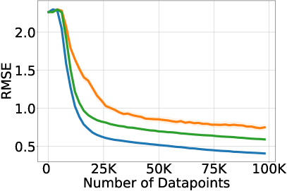
Figure 2: The mean RMSE of the models in the beta-rank-v1 (left) and ml-100k-v1 (right) environments averaged across $10$ runs. Shaded areas indicate $95\%$ confidence intervals. RMSE was evaluated with respect to a randomly sampled test set of size 100,000. Both cafl and Feedback observe their own recommendations, while Uniform observes randomly chosen user-item pairs. Lower RMSE is better.

Results.  As shown in Figs. 2 and 3, cafl increases the model’s predictive (RMSE) and ranking (NDCG) accuracy, when compared to the uncorrected version (Feedback).We note that the model that observes uniformly chosen datapoints (Uniform) still outperforms cafl in most cases. This is expected since the cafl correction is attempting to use the observed feedback data to approximate the empirical risk that Uniform observes. Uniform effectively observes more datapoints than cafl at any given timestep.

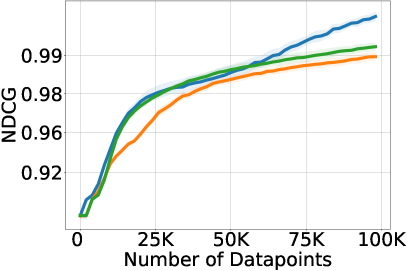
Figure 3: Left: The mean NDCG of the models averaged across all users and across $10$ runs in the beta-rank-v1 (left) and ml-100k-v1 (right) environments. Shaded areas indicate $95\%$ confidence intervals. NDCG was evaluated with respect to a randomly sampled test set of size 100,000. Both cafl and Feedback observe their own recommendations, while Uniform observes randomly chosen user-item pairs. We use a logit scale for the Y-axis for readability. Higher NDCG is better.

4.3 cafl, feedback loops, and homogenization

Recommendation systems and their feedback loops have been shown to homogenize the set of items that users will observe beyond what is necessary to achieve optimal utility (Chaney et al., 2018). This is troublesome since it implies algorithmic minutia may have an undeservedly large impact on the popularity of different items.

Here we evaluate the homogenization effect of uniform sampling, cafl, and the vanilla recommender with feedback loops. We show that cafl reduces homogenization when feedback loops induce homogenization. In settings where feedback loops do not induce homogenization (i.e. when feedback loops induce the same or less homogenization than uniform sampling), we show that the behavior of cafl tracks random sampling, suggesting that cafl breaks feedback loops in those settings too.

Evaluation metrics for homogenization.  We define homogenization as the mean similarity between every pair of users’ recommended items, for which we use the Jaccard coefficient as the measure of similarity between two different users $u_{1}$ and $u_{2}$:

$$S(u_{1},u_{2})=\frac{\sum_{i}\mathbf{\boldsymbol{A}}_{t,u_{1}i}\wedge\mathbf{\boldsymbol{A}}_{t,u_{2}i}}{\sum_{i}\mathbf{\boldsymbol{A}}_{t,u_{1}i}\vee\mathbf{\boldsymbol{A}}_{t,u_{2}i}}.$$

Results.  When feedback loops increase homogenization, cafl successfully mitigates homogenization. The right plot of Figure 4 shows the Jaccard index over time for the ml-100k-v1 environment. In this setting, feedback effects cause the uncorrected recommender system to further homogenize the user experience when compared to a recommender system that observes uniformly sampled data. cafl is able to reduce homogenization in this setting. We note that this outcome is not self-evident. In particular, the cafl correction only leads to a more accurate empirical risk estimate and does not explicitly consider homogenization.

Turning to the beta-rank-v1 homogenization results, we observe that cafl is unable to reduce homogenization when it is not caused by feedback effects. As shown in the left plot of Figure 4, cafl increased homogenization in this setting when compared to the uncorrected feedback recommender. Surprisingly, the uniform recommender also leads to higher homogenization. This suggests that homogenization is not always caused by feedback effects, since we would otherwise expect the feedback recommender to have the highest homogenization if that were the case. In fact, these results suggest that feedback can sometimes reduce homogenization.

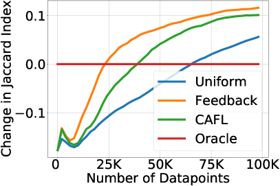
Figure 4: The mean Jaccard coefficient between the set of recommended items of each user-item pair at each timestep minus the Jaccard coefficient of an oracle recommender system on the beta-rank-v1 (left) and ml100k-v1 (right) environments. Both cafl and Feedback observe their own recommendations, while Uniform observes randomly chosen user-item pairs. Lower change in Jaccard index is better.

4.4 Comparison with Prior Work

We replicated the experimental setup of Pan et al. (2021) to compare cafl with prior correction methods. We evaluate cafl on a variation of the simulated environment first proposed by Chaney et al. (2018). In this setup if user $u$ interacts with item $i$ at time $t$ we have

$$R_{t,ui} \sim\mathrm{Beta}^{\prime}\left(\theta_{u}^{\top}\beta_{i}\right)$$

where $\mathrm{Beta}^{\prime}(\mu)$ is a reparametrized beta distribution with variance $\sigma^{2}=0.01$ that is equivalent to $Beta(a,b)$ where $a=\left(\frac{1-\mu}{\sigma^{2}}-\frac{1}{\mu}\right)\mu$ and $b=a\left(\frac{1}{\mu}-1\right)$. The latent user and item vectors have distribution

$$\theta_{u}\sim\mathrm{Dirichlet}(\mu_{\theta}), \quad\mu_{\theta}\sim\mathrm{Dirichlet}(\mathbf{20})$$

$$\beta_{i}\sim\mathrm{Dirichlet}(\mu_{\beta}), \quad\mu_{\beta}\sim\mathrm{Dirichlet}(\mathbf{100}).$$

We consider $U=3000$ users and $I=1000$ items. We sample one item for each user over $30$ timesteps, where items are selected uniformly at random when $t=1$ and for $t>1$ we have

$$P\left(A_{t,ui}=1\right)\propto\begin{cases}0&\text{ if user $u$ already interacted with item $i$}\\ 10&\text{ if }\mathrm{rank}_{t}(u,i)<=100\\ 1&\text{ otherwise},\end{cases}$$

where the ranking function $\mathrm{rank}_{t}(u,i)$ orders items from largest to smallest based on a score function intended to mimic the recommendation process:

$$\mathrm{score}_{t}(u,i)\propto\sum_{s=1}^{t-1}\sum_{j=1}^{I}A_{s,uj}R_{s,uj}\exp{(S_{ij})},$$

where $S_{ij}$ is an item-item similarity matrix with distribution

$$S_{ij}\sim\mathrm{Beta}^{\prime}\left(\beta_{i}^{\top}\beta_{j}\right).$$

We use the first $20$ sampled items for each user as the training set and do not consider the last $10$ for consistency with Pan et al. (2021). Finally, we sample an additional $20$ unobserved ratings uniformly at random for each user to create the test set.

We then train a generalized matrix factorization model (He et al., 2017) using Adam with identical hyperparameter settings to Pan et al. (2021) but with each observation in the training loss weighted according to cafl. We then evaluate the recommender’s predictions on the test set, repeating the entire simulation procedure $10$ times.

Correction	MSE	MAE
Naive	$2.001\pm 0.066$	$1.087\pm 0.021$
Pop	$1.990\pm 0.035$	$1.080\pm 0.010$
PF (Gopalan et al., 2015)	$1.945\pm 0.038$	$1.065\pm 0.010$
Pan (Pan et al., 2021)	$1.896\pm 0.042$	$1.042\pm 0.011$
cafl (This paper)	$\mathbf{1.818\pm 0.019}$	$\mathbf{1.015\pm 0.005}$

Table 1: Predictive performance (MSE and MAE) of generalized matrix factorization on a benchmark derived from a modification of the simulation proposed by Chaney et al. (2018) when trained with: no correction (Naive), a correction that scales inversely with item popularity (Pop), Poisson Factorization (PF), the correction by Pan et al. (2021) (Pan), and the correction algorithm proposed in this work (cafl).

Table 1 shows the performance of cafl averaged across all $10$ runs compared to the correction methods evaluated by Pan et al. (2021). cafl outperforms all prior methods both in terms of MSE and MAE. We observe that the improvement in MSE/MAE when comparing cafl to Pan is larger than the improvement in MSE/MAE when comparing Pan to Poisson Factorization. Furthermore, we note that the MSE gap between the simple popularity-based re-weighting scheme and Pan is equal to the MSE gap between cafl and Pan, indicating that the cafl algorithm proposed in this work leads to significant performance improvements.

5 Discussion

Feedback loops are endemic in multi-step recommender systems. Recommendations affect user behavior; which in turn affect future recommendations through the retraining process. Feedback loops in recommender systems bias the inference of user preferences, compromise recommendation quality, and can homogenize recommendations. To this end, we propose cafl, a causal adjustment algorithm that can provably break feedback loops. Across empirical studies, we find that cafl improves recommendation quality and mitigates negative feedback effects. It also significantly improves predictive performance when compared to prior correction methods.

Furthermore, our results on homogenization show the importance of isolating feedback effects when evaluating models in dynamic setting. Our results indicate that the model’s inductive bias and the number of datapoints, can sometimes have a stronger effect on homogenization than feedback loops. The picture of how and when homogenization occurs in recommender systems still remains incomplete. Future work that meticulously evaluates recommender systems in dynamic settings will likely shed light on this phenomenon.

Appendix

Appendix A Proofs

A.1 Proof of Theorem 2

Proof.

We decompose the causal objective into terms where positivity holds and those where positivity is violated:

$$L^{\mathrm{causal}}(\Theta)$$ (22)

$$=\frac{1}{t}\sum_{s=1}^{t}\sum_{u=1}^{U}\sum_{i=1}^{I}\mathbb{E}_{\mathbf{\boldsymbol{A}}_{s}}\left[\mathbb{E}_{P(R_{s,ui}\,|\,\mathrm{do}(A_{s,ui}=A_{s,ui}))}\left[\log P_{\Theta}\left(R_{s,ui}\,|\,A_{s,ui}\right)\right]\right]$$ (23)

$$=\sum_{s=1}^{t}c_{t}\left[\sum_{u=1}^{U}\sum_{i=1}^{I}\mathbb{E}_{\mathbf{\boldsymbol{A}}_{s}}\left[\mathbb{E}_{P(R_{s,ui}\,|\,\mathrm{do}(A_{s,ui}=A_{s,ui}))}\left[\log P_{\Theta}\left(R_{s,ui}\,|\,A_{s,ui}\right)\right]\right]\right]$$ (24)

$$=\sum_{s=1}^{t}c_{t}\left[\sum_{u=1}^{U}\sum_{i=1}^{I}\sum_{a_{s,ui}\in\{0,1\}}\mathbb{E}_{P(R_{s,ui}\,|\,\mathrm{do}(A_{s,ui}=a_{s,ui}))}\left[\mathbb{1}\{A_{s,ui}=a_{s,ui}\}\cdot\log P_{\Theta}\left(R_{s,ui}\,|\,A_{s,ui}\right)\right]\right]$$ (25)

$$=\sum_{s=1}^{t}c_{t}\left[\sum_{\begin{subarray}{c}u,i:\\ P(A_{s,ui}=\\ a_{s,ui}\,|\,\hat{\Theta}_{s-1})>0\end{subarray}}\sum_{a_{s,ui}\in\{0,1\}}\mathbb{E}_{P(R_{s,ui}\,|\,\mathrm{do}(A_{s,ui}=a_{s,ui}))}\left[\mathbb{1}\{A_{s,ui}=a_{s,ui}\}\cdot\log P_{\Theta}\left(R_{s,ui}\,|\,A_{s,ui}\right)\right]\right]$$

$$\quad+\sum_{s=1}^{t}c_{t}\left[\sum_{\begin{subarray}{c}u,i:\\ P(A_{s,ui}=\\ a_{s,ui}\,|\,\hat{\Theta}_{s-1})=0\end{subarray}}\sum_{a_{s,ui}\in\{0,1\}}\mathbb{E}_{P(R_{s,ui}\,|\,\mathrm{do}(A_{s,ui}=a_{s,ui}))}\left[\mathbb{1}\{A_{s,ui}=a_{s,ui}\}\cdot\log P_{\Theta}\left(R_{s,ui}\,|\,A_{s,ui}\right)\right]\right].$$ (26)

The first equation is due to Eq. 10; the second equation is due to the stationary assumption of intervention distributions (i.e. the second assumption of Theorem 2); the third equation is an unbiased estimator of the expectation over $\mathbf{\boldsymbol{A}}_{s}$; the fourth equation separates the loss into two terms, one where positivity holds and the other where positivity fails. $\hat{L}_{s,u,i}^{\mathrm{obs}}(\Theta\,;\,a_{s,ui})$ in the theorem is an unbiased estimator of the second term, following the same inverse probability argument as in Propositions 1 and 14. $\hat{L}_{s,u,i}^{\mathrm{unobs}}(\Theta\,;\,a_{s,ui})$ is an unbiased estimator of the first term due to the stationary assumption of intervention distributions, together with the inverse probability argument as in Propositions 1 and 14. ∎

References

- Bell and Koren [2007] Robert M Bell and Yehuda Koren. Scalable collaborative filtering with jointly derived neighborhood interpolation weights. In Seventh IEEE international conference on data mining (ICDM 2007), pages 43–52. IEEE, 2007.
- Bonner and Vasile [2018] Stephen Bonner and Flavian Vasile. Causal embeddings for recommendation. In Proceedings of the 12th ACM Conference on Recommender Systems, pages 104–112. ACM, 2018.
- Chakrabarti et al. [2006] Soumen Chakrabarti, Alan Frieze, and Juan Vera. The influence of search engines on preferential attachment. Internet Mathematics, 3(3):361–381, 2006.
- Chaney et al. [2018] Allison JB Chaney, Brandon M Stewart, and Barbara E Engelhardt. How algorithmic confounding in recommendation systems increases homogeneity and decreases utility. In Proceedings of the 12th ACM Conference on Recommender Systems, pages 224–232, 2018.
- Farquhar et al. [2021] Sebastian Farquhar, Yarin Gal, and Tom Rainforth. On statistical bias in active learning: How and when to fix it. arXiv preprint arXiv:2101.11665, 2021.
- Gopalan et al. [2015] Prem Gopalan, Jake M Hofman, and David M Blei. Scalable recommendation with hierarchical poisson factorization. In UAI, pages 326–335, 2015.
- Gopalan et al. [2014] Prem K Gopalan, Laurent Charlin, and David Blei. Content-based recommendations with poisson factorization. In Z. Ghahramani, M. Welling, C. Cortes, N.D. Lawrence, and K.Q. Weinberger, editors, Advances in Neural Information Processing Systems 27, pages 3176–3184. Curran Associates, Inc., 2014.
- Harper and Konstan [2015] F Maxwell Harper and Joseph A Konstan. The movielens datasets: History and context. ACM Transactions on Interactive Intelligent Systems (TIIS), 5(4):1–19, 2015.
- He et al. [2017] Xiangnan He, Lizi Liao, Hanwang Zhang, Liqiang Nie, Xia Hu, and Tat-Seng Chua. Neural collaborative filtering. In Proceedings of the 26th International Conference on World Wide Web, pages 173–182, 2017.
- Hernández-Lobato et al. [2014] José Miguel Hernández-Lobato, Neil Houlsby, and Zoubin Ghahramani. Probabilistic matrix factorization with non-random missing data. In International Conference on Machine Learning, pages 1512–1520. PMLR, 2014.
- Hosseinmardi et al. [2020] Homa Hosseinmardi, Amir Ghasemian, Aaron Clauset, David M Rothschild, Markus Mobius, and Duncan J Watts. Evaluating the scale, growth, and origins of right-wing echo chambers on youtube. arXiv preprint arXiv:2011.12843, 2020.
- Hu et al. [2008] Yifan Hu, Yehuda Koren, and Chris Volinsky. Collaborative filtering for implicit feedback datasets. In Data Mining, 2008. ICDM’08. Eighth IEEE International Conference on, pages 263–272. IEEE, 2008.
- Imbens and Rubin [2015] Guido W Imbens and Donald B Rubin. Causal inference in statistics, social, and biomedical sciences. Cambridge University Press, 2015.
- Jiang et al. [2019] Ray Jiang, Silvia Chiappa, Tor Lattimore, András György, and Pushmeet Kohli. Degenerate feedback loops in recommender systems. In Proceedings of the 2019 AAAI/ACM Conference on AI, Ethics, and Society, pages 383–390, 2019.
- Kalimeris et al. [2021] Dimitris Kalimeris, Smriti Bhagat, Shankar Kalyanaraman, and Udi Weinsberg. Preference amplification in recommender systems. In Proceedings of the 27th ACM SIGKDD Conference on Knowledge Discovery & Data Mining, pages 805–815, 2021.
- Koren [2009] Yehuda Koren. Collaborative filtering with temporal dynamics. In Proceedings of the 15th ACM SIGKDD International Conference on Knowledge Discovery and Data Mining, pages 447–456, 2009.
- Krauth et al. [2020] Karl Krauth, Sarah Dean, Alex Zhao, Wenshuo Guo, Mihaela Curmei, Benjamin Recht, and Michael I Jordan. Do offline metrics predict online performance in recommender systems? arXiv preprint arXiv:2011.07931, 2020.
- Lee et al. [2016] Joonseok Lee, Seungyeon Kim, Guy Lebanon, Yoram Singer, and Samy Bengio. LLORMA: Local low-rank matrix approximation. The Journal of Machine Learning Research (JMLR), 17(1):442–465, 2016.
- Liang et al. [2016] Dawen Liang, Laurent Charlin, James McInerney, and David M Blei. Modeling user exposure in recommendation. In Proceedings of the 25th International Conference on World Wide Web, pages 951–961. International World Wide Web Conferences Steering Committee, 2016.
- Liang et al. [2018] Dawen Liang, Rahul G Krishnan, Matthew D Hoffman, and Tony Jebara. Variational autoencoders for collaborative filtering. In Proceedings of the 2018 World Wide Web conference, pages 689–698, 2018.
- Mansoury et al. [2020] Masoud Mansoury, Himan Abdollahpouri, Mykola Pechenizkiy, Bamshad Mobasher, and Robin Burke. Feedback loop and bias amplification in recommender systems. In Proceedings of the 29th ACM International Conference on Information & Knowledge Management, pages 2145–2148, 2020.
- Marlin and Zemel [2009] Benjamin M Marlin and Richard S Zemel. Collaborative prediction and ranking with non-random missing data. In Proceedings of the third ACM conference on Recommender systems, pages 5–12. ACM, 2009.
- Mnih and Salakhutdinov [2008] Andriy Mnih and Ruslan R Salakhutdinov. Probabilistic matrix factorization. In Advances in Neural Information Processing Systems, pages 1257–1264, 2008.
- Ning and Karypis [2011] Xia Ning and George Karypis. Slim: Sparse linear methods for top-n recommender systems. In 2011 IEEE 11th International Conference on Data Mining, pages 497–506. IEEE, 2011.
- Pan et al. [2021] Weishen Pan, Sen Cui, Hongyi Wen, Kun Chen, Changshui Zhang, and Fei Wang. Correcting the user feedback-loop bias for recommendation systems. arXiv preprint arXiv:2109.06037, 2021.
- Pearl [2009] Judea Pearl. Causality. Cambridge University Press, 2009.
- Perdomo et al. [2020] Juan Perdomo, Tijana Zrnic, Celestine Mendler-Dünner, and Moritz Hardt. Performative prediction. In International Conference on Machine Learning, pages 7599–7609. PMLR, 2020.
- Rendle [2012] Steffen Rendle. Factorization machines with libFM. ACM Transactions on Intelligent Systems and Technology, 3(3):57:1–57:22, May 2012. ISSN 2157-6904.
- Salganik et al. [2006] Matthew J Salganik, Peter Sheridan Dodds, and Duncan J Watts. Experimental study of inequality and unpredictability in an artificial cultural market. Science, 311(5762):854–856, 2006.
- Schmit and Riquelme [2018] Sven Schmit and Carlos Riquelme. Human interaction with recommendation systems. In International Conference on Artificial Intelligence and Statistics, pages 862–870. PMLR, 2018.
- Schnabel et al. [2016] Tobias Schnabel, Adith Swaminathan, Ashudeep Singh, Navin Chandak, and Thorsten Joachims. Recommendations as treatments: Debiasing learning and evaluation. In International Conference on Machine Learning, pages 1670–1679. PMLR, 2016.
- Sedhain et al. [2015] Suvash Sedhain, Aditya Krishna Menon, Scott Sanner, and Lexing Xie. Autorec: Autoencoders meet collaborative filtering. In The World Wide Web Conference, pages 111–112, 2015.
- Sharma et al. [2015] Amit Sharma, Jake M Hofman, and Duncan J Watts. Estimating the causal impact of recommendation systems from observational data. In Proceedings of the Sixteenth ACM Conference on Economics and Computation, pages 453–470. ACM, 2015.
- Sinha et al. [2016] Ayan Sinha, David F Gleich, and Karthik Ramani. Deconvolving feedback loops in recommender systems. Advances in Neural Information Processing Systems, 29:3243–3251, 2016.
- Steck [2019] Harald Steck. Embarrassingly shallow autoencoders for sparse data. In The World Wide Web Conference, pages 3251–3257, 2019.
- Sun et al. [2019] Wenlong Sun, Sami Khenissi, Olfa Nasraoui, and Patrick Shafto. Debiasing the human-recommender system feedback loop in collaborative filtering. In Companion Proceedings of The 2019 World Wide Web Conference, pages 645–651, 2019.
- Wang et al. [2006] Jun Wang, Arjen P De Vries, and Marcel JT Reinders. Unifying user-based and item-based collaborative filtering approaches by similarity fusion. In International ACM SIGIR Conference on Research and Development in Information Retrieval, pages 501–508, 2006.
- Wang et al. [2019] Yixin Wang, Dhanya Sridhar, and David M Blei. Equal opportunity and affirmative action via counterfactual predictions. arXiv preprint arXiv:1905.10870, 2019.
- Wang et al. [2020] Yixin Wang, Dawen Liang, Laurent Charlin, and David M Blei. Causal inference for recommender systems. In Fourteenth ACM Conference on Recommender Systems, pages 426–431, 2020.
- Zheng et al. [2016] Yin Zheng, Bangsheng Tang, Wenkui Ding, and Hanning Zhou. A neural autoregressive approach to collaborative filtering. arXiv preprint arXiv:1605.09477, 2016.