Galaxy number-count dipole and superhorizon fluctuations

Abstract

In view of the growing tension between the dipole anisotropy of number counts of cosmologically distant sources and of the cosmic microwave background (CMB), we investigate the number count dipole induced by primordial perturbations with wavelength comparable to or exceeding the Hubble radius today. First, we find that neither adiabatic nor isocurvature superhorizon modes can generate an intrinsic number count dipole. However a superhorizon isocurvature mode does induce a relative velocity between the CMB and the (dark) matter rest frames and thereby affects the CMB dipole. We revisit the possibility that it has an intrinsic component due to such a mode, thus enabling consistency with the galaxy number count dipole if the latter is actually kinematic in origin. Although this scenario is not particularly natural, there are possible links with other anomalies and it predicts a concommitant galaxy number count quadrupole which may be measurable in future surveys. We also investigate the number count dipole induced by modes smaller than the Hubble radius, finding that subject to CMB constraints this is too small to reconcile the dipole tension.

I Introduction

Despite great advances in cosmology, we have yet to confirm whether the cosmic rest frame (CRF) of galaxies and dark matter in which they are isotropically distributed on the sky, actually coincides with that of the Cosmic Microwave Background (CMB). Ellis & Baldwin [1] were the first to note that this is a powerful consistency test of the Friedman-Lemaître-Robertson-Walker (FLRW) models, in which the two CRFs must coincide. If the observed CMB dipole anisotropy is indeed kinematic due to our local peculiar motion with respect to the CRF [2], then there must be a corresponding kinematic dipole imprinted in the galaxy number counts on the sky.

It is only recently that large enough galaxy samples have become available to perform this test [3, 4, 5, 6, 7, 8]. Interestingly, there is growing evidence that the two CRFs do not coincide [9, 10, 11, 12, 13, 14, 15, 16, 17, 18, 19, 20] thus challenging the fundamental basis of the standard $\Lambda$CDM cosmology. In fact distant radio galaxies and quasars exhibit a dipole 2–3 times higher than expected from the kinematic interpretation of CMB dipole, with the highest reported tension now exceeding $5\sigma$ [20, 21].

The dipole test [1] is sometimes referred to as a test of the Cosmological Principle [20, 22]. However we must first rule out that the dipole mismatch is not due to any large-scale inhomogeneity compatible with a perturbed FLRW model before abandoning this foundational assumption of the standard cosmology, upon which the inference that the universe is dominated today by a Cosmological constant $\Lambda$ rests [23]. After all, apart from its dipole, the CMB has only small anisotropies of ${\cal O}(10^{-5})$ [24, 25], and peculiar velocities are of ${\cal O}(10^{-3}c)$ i.e. well within the validity of cosmological perturbation theory. In fact it is quite possible that (dark) matter has a relative velocity with respect to the CMB, which is often a signature of isocurvature fluctuations [26, 27, 28, 29, 30]. Moreover, the dipole tension appears only if we assume that there are no intrinsic (non-kinematic) components to either dipole. This is a strong assumption which requires scrutiny. While the kinematic interpretation of the CMB dipole is consistent with other tests [31, 32, 33], these do not exclude the possibility of an intrinsic dipole [34, 35, 36]. This motivates our investigation of whether the dipole tension can be explained by inhomogeneities larger than the present horizon.

Turner [29, 28] (see also Ref. [37]) suggested that a superhorizon isocurvature fluctuation can provide an intrinsic dipole modulation to the CMB and called it a “tilted universe” to express that it would look as if galaxies have a global motion with respect to the CMB rest frame. The effects of superhorizon fluctuations on the CMB have subsequently been studied in detail [38, 39, 40, 41, 42] and it is established that only isocurvature modes induce a CMB dipole at leading order. In this work, we also study the effect on the galaxy number count dipole using the formalism developed in Refs. [43, 44, 45, 46]. Related work may be found in Refs. [47, 48, 49].

It is important to explore such new physics also in view of other reported anomalies and tensions within $\Lambda$CDM (see e.g. Refs. [50, 51, 52] for recent reviews). For example, the effects of a local void on the CMB dipole have been discussed  [53, 54, 55]. The presence of superhorizon modes is an interesting possibility in itself as they may be pre-inflationary remnants and for the mode to not have been diluted away, inflation must have lasted for just long enough to create our present Hubble patch. This scenario fits well within open inflation models wherein our observable universe results from bubble nucleation in false vacuum [57, 58, 59, 60, 61]. Furthermore, isocurvature fluctuations typically arise in the presence of light scalar fields during inflation [62, 63, 64]. This applies, for instance, to axions [65, 66, 67, 68] (see, e.g., Refs. [69, 70] for recent reviews of axion cosmology), or more generically to curvatons [71, 72, 73]. A variation of the mean value of the axion field across the observable universe is then interpreted as a discrete superhorizon mode [40].

This paper is organised as follows. In § II we provide a derivation of the effect of superhorizon modes on galaxy number counts, complementary to that in Ref. [43]. In § III we study the number count fluctuations in the presence of adiabatic and cold dark matter (CDM) isocurvature modes, and also their effects on CMB temperature fluctuations. In § IV we apply such considerations to the current dipole tension. In § V we consider the effect on the number count dipole of modes which are sub-horizon today but were superhorizon at the time of decoupling. We conclude and discuss further directions in § VI. Details of our calculations are provided in the Appendices. We work throughout in reduced Planck units ($8\pi G=c=1$) unless otherwise stated.

II Galaxy number count: review and complementary derivation

We start by computing the general relativistic galaxy number count fluctuations following the covariant formulation of Ellis [74] and Kasai & Sasaki [43]. In Appendix B we compare our formulation with other recent works [45, 46, 22] and show that they are exactly equivalent. An improvement we make is in not dropping any monopole or dipole terms at the Observer’s position.

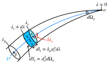
Figure 1: A source at $s$ emits photons which reach us at $o$ along null geodesics $k^{\mu}$ parameterised by the affine parameter $\lambda$. Due to the source velocity $u^{\mu}_{s}$, the photon has a spatial displacement $dl_{s}$ following an infinitesimal change in the affine parameter $d\lambda$. The observed infinitesimal volume is $dV_{s}=dl_{s}dS_{s}$ and the cross-section $dS_{s}$ of the photon bundle defines the Observer’s area distance $d_{o}$. A fixed affine parameter $\lambda_{s}$ hypersurface is related to a fixed redshift $z$ hypersurface by shifting the affine parameter of the source by $\delta\lambda_{s}$. There may also be another source $g$ beyond $s$. The total number count $N$ per solid angle at $o$ is the integral along the whole photon bundle. (After Figure 8 in Ellis [74].)

Consider sources of number density $\hat{n}_{s}$, with given 4-velocity $\hat{u}_{s}^{\mu}$ at a given point $s$ in a perturbed flat FLRW universe with metric $\hat{g}_{\mu\nu}$. For the moment, we assume that $\hat{n}_{s}$ is a function of time only. The sources emit photons with 4-momentum $\hat{k}^{\mu}$, which travel along null geodesics parametrised by an affine parameter $\hat{\lambda}$ and reach our location at a point $o$ from a direction $\hat{n}$. We are moving with 4-velocity $\hat{u}_{o}^{\mu}$ so the number of sources we see at point $o$ within the distance $d\hat{l}_{s}$, travelled by a photon after an infinitesimal change in the affine parameter $d\hat{\lambda}$, is [74]

$$dN(\hat{\lambda},\hat{n})=\hat{n}_{s}\,d\hat{l}_{s}d\hat{S}_{s}\,,$$ (1)

where $d\hat{S}_{s}$ is the cross-sectional area of the photon bundle at $s$. The cross-sectional area $d\hat{S}_{s}$ observed at $o$ is independent of the Observer’s velocity $\hat{u}_{o}^{\mu}$ if the latter is $\ll c$ [74]. The spatial displacement of the photon after $d\hat{\lambda}$ is $d\hat{l}_{s}=(-\hat{k}_{\mu}\hat{u}_{s}^{\mu})d\hat{\lambda}$, where $\hat{\omega}=-\hat{k}_{\mu}\hat{u}_{s}^{\mu}$ is the energy of the photon. Then the change of the cross-sectional area along the null geodesics is [74]

$$\frac{d}{d\hat{\lambda}}(d\hat{S}_{s})=d\hat{S}_{s}\hat{\nabla}_{\mu}\hat{k}^{\mu}\,.$$ (2)

The cross-sectional area is used to define the Observer’s area distance $\hat{d}_{o}$ by $d\hat{S}_{s}={\hat{d}}_{o}^{2}d\Omega_{o}$ where $d\Omega_{o}$ is the solid angle of the photon bundle at the Observer’s position. Before showing the equations for $\hat{k}^{\mu}$ and $\hat{d}_{o}$, it is more convenient to to work with conformally rescaled variables given by

$$\hat{g}_{\mu\nu}=a^{2}g_{\mu\nu}\quad ,\quad d\hat{\lambda}=-a^{2}d\lambda\quad,\quad\hat{k}^{\mu}=-a^{-2}k^{\mu}$$ (3)

$$\hat{u}^{\mu}=a^{-1}u^{\mu}\quad,\quad\hat{d}_{o} =a\,d_{o}\quad{,}\quad\hat{n}_{s}=a^{-3}n_{s}\quad{\rm and}\quad\hat{\omega}=a^{-1}\omega=a^{-1}k_{\mu}u_{s}^{\mu}\,.$$ (4)

In these variables, we have:

$$dN(\lambda,\hat{n})=n_{s}\omega d_{o}^{2}d\lambda d\Omega_{o}\,,$$ (5)

with all the arguments above evaluated at a point parameterised by $(\lambda,\hat{n})$. The equations necesssary to solve the system are the null geodesics equation, the Raychaudhuri equation for null geodesics, and the change of cross sectional area, respectively [43]

$$\frac{dk^{\alpha}}{d\lambda} =-\Gamma^{\alpha}_{\mu\nu}k^{\mu}k^{\nu}\,,$$ (6)

$$\frac{dd_{o}}{d\lambda} =\frac{1}{2}\theta d_{o}\,,$$ (7)

$$\frac{d\theta}{d\lambda} =-R_{\mu\nu}k^{\mu}k^{\nu}-\frac{1}{2}\theta^{2}-\sigma^{\mu\nu}\sigma_{\mu\nu}\,,$$ (8)

where $\theta\equiv\nabla_{\mu}k^{\mu}$ and $\sigma_{\mu\nu}$ are respectively the expansion scalar and the shear of the congruence of null geodesics [75]. Note that due to the conformal invariance of null geodesics, the equations for the original variables would look exactly the same as Eqs. (6)-(8) but all with “hatted” quantities. Also we use the subscripts $s$ and $o$ to respectively denote evaluation at the Source and Observer positions, except for $d_{o}$ which denotes the area distance to the Source measured by the Observer. This means that for $\lambda$, the affine parameter of the past directed null geodesics, we have $\lambda_{o}=0$. Alternatively, $\lambda=0$ means that the Observer is on top of the Source.

II.1 Number count fluctuations due to cosmological perturbations

We proceed to derive the galaxy number count fluctuations under the effects of cosmological perturbations. We present the main formulae here and provide the details in Appendix A. We perturb the variables as follows. First, following Kasai & Sasaki [43], we denote all perturbed variables with a tilde, e.g., $\tilde{g}_{\mu\nu}$ is the perturbed metric and $g_{\mu\nu}$ is the background one. For simplicity, we neglect any vector or tensor perturbation. We work in a perturbed flat FLRW metric in conformal coordinates $(\eta,x^{i})$ and in the shear free gauge, viz.

$$\tilde{g}_{\mu\nu}=\eta_{\mu\nu}+\delta g_{\mu\nu},\quad{\rm where}\quad\delta g_{\mu\nu}=-2\Psi\delta^{0}_{(\mu}\delta^{0}_{\nu)}+2\Phi\delta_{ij}\delta^{i}_{(\mu}\delta^{j}_{\nu)}\,.$$ (9)

The 4-velocities of the Source and the Observer read respectively:

$$\tilde{u}_{s/o}^{\mu}=(1-\Psi_{s/o})\delta^{\mu}_{0}+v_{s/o}^{i}\delta^{\mu}_{i}\,.$$ (10)

Similarly, we have:

$$\tilde{k}^{\mu}=k^{\mu}+\delta k^{\mu}\quad ,\quad\tilde{\omega}=1+\delta\omega\,,$$ (11)

$$\tilde{d}_{o}=d_{o}(1+\delta_{r})\quad,\quad\tilde{n}_{s}=n_{s} (1+\delta_{n})\quad{\rm and}\quad\tilde{\eta}=\eta+\delta\eta\,.$$ (12)

The form of $\delta k^{\mu}$, $\delta_{r}$, $\delta\omega$ and $\delta\eta$ in terms of $\Phi$, $\Psi$ and $v_{s/o}^{i}$ are given by the solutions to Eqs. (6)-(8). Note that without loss of generality we have normalised the constant energy of the photon to unity, i.e. $\omega=1$, since the null geodesics do not depend on the photon energy and we are only interested in relative changes in number counts. We present the solutions below and refer the reader to Appendix A for more details.

Before proceeding further, it is important to note that up to this point we worked in terms of the affine parameter $\lambda$. However, observations are made at a fixed redshift $z=\hat{\omega}_{s}/\hat{\omega}_{o}=(a_{o}\omega_{s})/(a_{s}\omega_{o})$ and not at a fixed $\lambda$. This means that we base our observations on a measured $\tilde{z}$ and then associate a “background” redshift $z=a_{o}/a_{s}$ to it. We take this into account by introducing a shift $\delta\lambda_{s}$ to the affine parameter $\lambda_{s}$ of the Source due to cosmological perturbations, which is defined by

$$1+\tilde{z}(\lambda_{s}+\delta\lambda_{s})\equiv 1+z(\lambda_{s})\,.$$ (13)

With the perturbation expansions (11) & (13) we find that the total number of sources up to redshift $z$ per unit solid angle is given by

$$\frac{d\tilde{N}(z,\hat{n})}{d\Omega_{o}} =\int_{0}^{\lambda_{s}+\delta\lambda_{s}}d\lambda\,\tilde{n}_{s}\tilde{\omega}_{s}\tilde{d}_{o}^{2}$$

$$=\int_{0}^{\lambda_{s}}d\lambda\,n_{s}d_{o}^{2}+n_{s}d_{o}^{2}(\lambda_{s})\delta\lambda_{s}+\int_{0}^{\lambda_{s}}d\lambda\,n_{s}d_{o}^{2}\left(\delta_{n}+2\delta_{r}+\delta\omega_{s}\right)\,.$$ (14)

Note that in Eq. (II.1), $\lambda_{s}$ is as in the background relation $z(\lambda_{s})$. We use this notation henceforth.

While Eq. (II.1) is what current observations measure, we expect that redshift tomography would be possible in future surveys. In anticipation, we compute the number count fluctuations of galaxies per redshift bin, and per solid angle viz.

$$\Delta_{n}(z_{s},\hat{n})\equiv\left(\frac{dN(z_{s},\hat{n})}{dz_{s}d\Omega_{o}}\right)^{-1}\left({\frac{d\tilde{N}(z_{s},\hat{n})}{dz_{s}d\Omega_{o}}-\frac{dN(z_{s},\hat{n})}{dz_{s}d\Omega_{o}}}\right)\,.$$ (15)

Eq. (15) is also the quantity considered in Refs. [45, 46]. A straightforward expansion of the derivative of Eq. (II.1) with respect to $\lambda_{s}$ yields

$$\Delta_{n}(z_{s},\hat{n})=2\frac{d\ln d_{o}}{d\lambda_{s}}\delta\lambda_{s}+\frac{d\delta\lambda_{s}}{d\lambda_{s}}+\delta_{n,s}+2\delta_{r,s}+\delta\omega_{s}\,,$$ (16)

where, for the moment, we consider $n_{s}$ to be constant.

We present below the solutions to Eqs (6)-(8) at the background level and at first-order in perturbation theory. The details are presented in Appendix A. First, we find at the background level, and along the line of sight, that

$$k^{\mu}=(-1,n^{i})\quad,\quad{\eta=\eta_{o}-\lambda}\quad{\rm and}\quad d_{o}(\lambda)=r(\lambda)=\lambda\,,$$ (17)

where $n^{i}$ is the direction of observation of the photon in the comoving radial direction $r$ from the Observer. Then, the first-order solutions read

$$\delta\omega_{s} =\Psi_{o}-\Psi_{s}+n_{i}v_{s}^{i}-n_{i}v_{o}^{i}-\int_{0}^{\lambda_{s}}d\lambda_{1}\frac{\partial}{\partial\eta}(\Psi-\Phi)\,,$$ (18)

$$\delta\eta_{s} =\lambda_{s}(n_{i}v^{i}_{o}-\Psi_{o})+2\int_{0}^{\lambda_{s}}d\lambda_{1}\Psi+\int_{0}^{\lambda_{s}}d\lambda_{1}\int_{0}^{\lambda_{1}}d\lambda_{2}\frac{\partial}{\partial\eta}(\Psi-\Phi)\,,$$ (19)

$$\delta\lambda_{s} =\delta\eta_{s}-\frac{\delta\omega_{s}}{{\cal H}_{s}}\,,$$ (20)

$$\delta_{r,s} =\Phi_{o}+\int_{0}^{\lambda_{s}}\frac{d\lambda_{1}}{r^{2}(\lambda_{1})}\int_{0}^{\lambda_{1}}d\lambda_{2}\,r^{2}(\lambda_{2})$$

$$\hskip 56.9055pt\times\left\{\frac{\partial^{2}}{\partial\eta^{2}}\Phi-2\frac{\partial}{\partial\eta}\frac{\partial}{\partial r}\Phi-\frac{1}{2}\Delta(\Psi-\Phi)+\frac{1}{2}\frac{\partial^{2}}{\partial r^{2}}(\Psi+\Phi)\right\}\,,$$ (21)

where $\Delta\equiv\partial_{i}\partial^{i}$ is the spatial Laplacian. We have set the conditions at the Observer’s position to be $\delta\omega_{o}=\delta\eta_{o}=\delta_{r,o}=0$. Any constant $\delta\eta_{o}$ and $\delta_{r,o}$ can be respectively reabsorbed by a constant shift in the time coordinate and in the affine parameter. The condition $\delta\omega_{o}=0$ means that there is no change in the observed photon energy if we are on top of the Source. Eq. (II.1), together with Eqs. (18)-(II.1) complete our derivation of the number count fluctuations.

II.2 Corrections due to flux threshold and evolution of sources

So far we have derived the galaxy number count in a perturbed flat FLRW universe assuming that the galaxy comoving number density is constant, and that galaxies have a monochromatic spectrum. However, in actual surveys we usually count the number of galaxies above some flux threshold $F_{*}$:

$$\hat{\cal N}_{s}(z,F>F_{*})=\int_{L_{s}(z,F)}^{\infty}\,dL\,\hat{n}_{s}(z,\ln L)\,,$$ (22)

where $L_{s}$ is the source luminosity given by

$$L_{s}=4\pi F\hat{d}_{o}^{2}(1+z)^{4}=4\pi F\tilde{d}_{o}^{2}a^{2}(\tilde{\eta})(1+\tilde{z})^{4}\,.$$ (23)

To find the effect of cosmological perturbations, we define $d{\cal N}$ as $dN$ in Eq. (II.1) and replace $n_{s}$ by ${\cal N}_{s}$. Proceeding as before we obtain

$$\frac{d{\cal N}(z,\hat{n})}{d\Omega_{o}} =\int_{0}^{\lambda_{s}+\delta\lambda_{s}}d\lambda\,\tilde{\cal N}_{s}(\tilde{\eta},\tilde{L})\tilde{\omega}\tilde{d}_{o}^{2}$$

$$=\int_{0}^{\lambda_{s}}d\lambda\,{\cal N}_{s}(\eta,L)r^{2}+{\cal N}_{s}(\eta,L)r^{2}(\lambda_{s})\delta\lambda_{s}$$

$$\hskip 28.45274pt+\int_{0}^{\lambda_{s}}d\lambda\,{\cal N}_{s}r^{2}\left(\delta_{n}+2\delta_{r}+\delta\omega+\frac{\partial\ln{\cal N}_{s}}{\partial\eta}\delta\eta+\frac{\partial\ln{\cal N}_{s}}{\partial\ln L}\delta\ln L\right)\,,$$ (24)

where we treated $\eta$ and $\ln L$ as separate variables. From Eq. (23) we have that $\delta\ln L=2\delta_{r}+2{\cal H}\delta\eta_{s}-4{\cal H}\delta\lambda_{s}$. Taking the derivative of Eq. (II.2) with respect to the redshift along the null geodesics, we arrive at

$$\Delta_{{\cal N}}(z_{s},\hat{n})= \left(\frac{\partial\ln{\cal N}_{s}}{\partial\ln(1+z_{s})}-2\frac{\partial\ln{\cal N}_{s}}{\partial\ln L}\right){\cal H}_{s}\left(\delta\lambda_{s}-\delta\eta_{s}\right)$$

$$+2\frac{\partial\ln{\cal N}_{s}}{\partial\ln L}\left(\frac{d\ln r}{d\lambda_{s}}\delta\lambda_{s}+\delta_{r}\right)+2\frac{d\ln r}{d\lambda_{s}}\delta\lambda_{s}+\frac{d\delta\lambda_{s}}{d\lambda_{s}}+\delta_{n}+2\delta_{r,s}+\delta\omega_{s}\,.$$ (25)

To compare with observations we define, as in previous work, the magnitude distribution index and ‘evolution bias’, respectively:

$$x\equiv-\frac{\partial\ln{\cal N}_{s}}{\partial\ln L}\quad{\rm and}\quad f_{\rm evo}\equiv-\frac{\partial\ln{\cal N}_{s}}{\partial\ln(1+z_{s})}\,.$$ (26)

For practical purposes, it is more convenient to work with the number density fluctuations in the comoving matter slicing $\delta_{n{\rm c}}$, which are related to the number density fluctuations in the shear free slicing $\delta_{n}$ as [76, 22]:

$$\delta_{n}=\delta_{n{\rm c}}+\frac{\partial\ln\hat{\cal N}_{s}}{\partial\eta}v_{s}=b(z)\delta_{m{\rm c}}+(3-f_{\rm evo}){\cal H}_{s}v_{s}\,,$$ (27)

where we used that $v_{s}^{i}=\partial^{i}v_{s}$. In Eq. (27) we have introduced the linear bias factor $b(z)$, making the usual assumption that the comoving galaxy number count fluctuations $\delta_{n{\rm c}}$ are proportional to the fluctuations $\delta_{m{\rm c}}$ in the CDM. The advantage of working with the former rather than the latter is that $\delta_{n{\rm c}}$ vanishes for superhorizon adiabatic fluctuations, making it convenient to set initial conditions in the early universe. With Eqs. (26) and (27), we rewrite Eq. (II.2) as

$$\Delta_{{\cal N}}(z_{s},\hat{n})= \Delta^{\delta}_{n}-2x(z)\Delta^{x}_{n}-f_{\rm evo}(z)\Delta^{\rm evo}_{n}\,,$$ (28)

where we defined

$$\Delta^{\delta}_{n}=b(z)\delta_{mc}+2\frac{\delta\lambda_{s}}{\lambda_{s}}+2\delta_{r,s}+\frac{d\delta\lambda_{s}}{d\lambda_{s}}+3{\cal H}_{s}v_{s}+\delta\omega_{s}\,,$$ (29)

$$\Delta_{n}^{x}=\delta\omega_{s}+\frac{\delta\lambda_{s}}{\lambda_{s}}+\delta_{r,s}\,,$$ (30)

$$\Delta_{n}^{\rm evo}={\cal H}_{s}v_{s}-\delta\omega_{s}\,.$$ (31)

The purpose of the separation in Eq. (28) is that in the next section we compute the three terms $\Delta^{\delta}_{n}$, $\Delta_{n}^{x}$ and $\Delta_{n}^{\rm evo}$, independently of $b(z)$, $x(z)$ and $f_{\rm evo}(z)$, which are harder to determine directly.

II.3 Kinematic dipole

First we consider the dipole due to our local motion. The kinematic dipole due to the velocity $v_{o}$ in $\Delta_{\cal N}$ is given by

$$d^{\rm kin}_{n}=\left(2+\frac{{\cal H}^{\prime}_{s}}{{\cal H}_{s}^{2}}+\frac{2-5s}{r_{s}{\cal H}_{s}}-f_{\rm evo}\right)\beta\,,$$ (32)

where $\beta\equiv n_{i}v^{i}_{o}$. The dipole in total number count ${\cal N}$ is then

$$d^{\rm kin}_{\cal N} =\frac{1}{\int_{0}^{\lambda_{s}}{\cal N}_{s}(\lambda,L)r^{2}d\lambda}\int_{0}^{\lambda_{s}}D^{\rm kin}_{n}{\cal N}_{s}(\lambda,L)r^{2}d\lambda$$ (33)

$$=\frac{1}{\int_{0}^{\lambda_{s}}{\cal N}_{s}(\lambda,L)r^{2}d\lambda}\int_{0}^{\lambda_{s}}\left(2+\frac{{\cal H}^{\prime}}{{\cal H}^{2}}+\frac{2(1-x)}{r{\cal H}}+\frac{\partial\ln{\cal N}_{s}}{\partial\ln(1+z)}\right)\beta{\cal N}_{s}(\lambda,L)r^{2}d\lambda\,.$$ (34)

As explained in Appendix B of Ref. [22], we can perform the integral above by looking for total derivatives, for instance we can use that

$$\frac{\partial\ln{\cal N}_{s}}{\partial\ln(1+z)} =\frac{d\ln{\cal N}_{s}}{d\ln(1+z)}-\frac{\partial\ln{\cal N}_{s}}{\partial\ln L}\frac{\partial\ln L}{\partial\ln(1+z)}=\frac{1}{{\cal H}}\frac{d\ln{\cal N}}{d\lambda}+x\left({1+\alpha}+\frac{2}{r{\cal H}}\right)\,,$$ (35)

where we have made the usual assumption that the sources have a power-law spectrum: $L(\nu)\propto\nu^{-\alpha}$. After integration, we obtain

$$d^{\rm kin}_{\cal N} =\frac{1}{\int_{0}^{\lambda_{s}}{\cal N}_{s}(\lambda,L)r^{2}d\lambda}\int_{0}^{\lambda_{s}}\left(2+x(1+\alpha)+\frac{1}{{\cal H}}\frac{d}{d\lambda}\ln\left(\frac{r^{2}{\cal N}_{s}}{{\cal H}}\right)\right)\beta{\cal N}_{s}(\lambda,L)r^{2}d\lambda$$ (36)

$$\qquad\qquad=\left(2+x(1+\alpha)\right)\beta+\frac{1}{\int_{0}^{\lambda_{s}}{\cal N}_{s}(\lambda,L)r^{2}d\lambda}\frac{r_{s}^{2}{\cal N}_{s}}{{\cal H}_{s}}\beta\,.$$ (37)

If we focus on the second term of Eq. (37) and rewrite it in terms of redshift, we find

$$\frac{1}{\int_{0}^{\lambda_{s}}{\cal N}_{s}(\lambda,L)r^{2}d\lambda}\frac{r_{s}^{2}{\cal N}_{s}}{{\cal H}_{s}}\beta\simeq\frac{\beta}{2}\frac{{\cal N}_{s}(z_{s},L(z_{s}))}{\int^{\eta_{0}}_{\eta_{s}}{\cal N}_{s}(\eta,L(\eta))\left(1-{\eta}/{\eta_{0}}\right)^{2}d(\eta/\eta_{0})}\frac{\left(1-(1+z_{s})^{-1/2}\right)^{2}}{(1+z_{s})^{1/2}}\,,$$ (38)

where we have approximated ${\eta}/\eta_{0}\simeq(1+z)^{-1/2}$, neglecting the effect of $\Lambda$ for analytical simplicity. Hence if ${\cal N}_{s}(z,L(z))\propto(1+z)^{\gamma}$ with $\gamma<1/2$, this term (38) quickly becomes negligible.

We check if this is indeed the case using the actual redshift distribution of the CatWISE quasars [20] shown in Fig. 2 and using the formulae for a matter+$\Lambda$ universe given in Appendix C.1. We find that the second term in Eq. (37) is $<10^{-3}\beta$, hence we recover the standard result [1]:

$$d^{\rm kin}_{\cal N} =\left(2+x(1+\alpha)\right)\beta\,.$$ (39)

For the CatWISE catalogue of quasars [20], $\langle x\rangle\simeq 1.7$ and $\langle\alpha\rangle\simeq 1.26$. So if the number count dipole and the CMB dipole are both solely due to our local motion, the amplitude of the number count dipole should be about 4 times that of the CMB. However, $d^{\rm kin}_{\cal N}$ is actually found to be a factor of over 2 larger than the expected value [20]. In the second step of Eq. (37) we assumed that $x$ and $\alpha$ are uncorrelated. In general this might not be the case as pointed out by Dalang & Bonvin [77]. However this has been directly demonstrated to be inconsequential for the CatWISE quasars [21] hence we do not consider this possibility further. In the next sections, we investigate whether superhorizon perturbations can indeed be the source of the above mismatch between the expected and found dipole.

Figure 2: Normalised PDF of the CatWISE quasar sample in redshift from Ref.[20]; the comoving number ${\cal N}_{s}(z)$ is proportional to this PDF times $(1+z)^{-3}$. The PDF is fitted with two log-normal distributions as $P(z)=\left(0.3/\sqrt{2\pi\,\Delta_{1}^{2}}\right)\exp\left(\log^{2}[z/0.3]/2\Delta_{1}^{2}\right)+\left(0.83/\sqrt{2\pi\,\Delta_{2}^{2}}\right)\exp\left(-\log^{2}[z]/2\Delta_{2}^{2}\right)$, with $\Delta_{1}=0.37$ and $\Delta_{2}=0.42$. Since the tail of the distribution falls off exponentially, the term (38) quickly becomes negligible.

III The effect of superhorizon perturbations today

We proceed to study the effect of superhorizon modes on the number count fluctuations above some flux limit (28). We also review the effect on the CMB temperature fluctuations as the constraints from CMB observations play a crucial role. However, before going into the details of the calculations, it is helpful to briefly review the possible initial conditions in the early universe and the evolution of superhorizon fluctuations until the present day. For analytical tractablility, we consider the expansion history of the universe in terms of known analytical solutions, i.e. we separately treat a radiation + matter universe and a matter + $\Lambda$ universe. The former is important for the CMB fluctuations and the latter for the number count fluctuations. In this section, we neglect baryons for simplicity and use the best-fit Planck values [78] for various parameters: $z_{\rm eq}\simeq 3400$, $z_{\rm dec}\simeq 1090$, ${\cal H}_{\rm eq}=k_{\rm eq}\simeq 0.0104\,{\rm Mpc}^{-1}$, ${\cal H}_{\rm dec}=k_{\rm dec}\simeq 4.8\times 10^{-3}\,{\rm Mpc}^{-1}$, $H_{0}\simeq 67.4\,{\rm km/s/Mpc}\simeq 2.2\times 10^{-4}\,{\rm Mpc}^{-1}$, $\Omega_{{\rm m},0}\simeq 0.315$ and $\Omega_{\Lambda,0}\simeq 0.685$. Also, from now on, we split our velocity (or the Sun’s velocity $v_{\odot}^{i}$) into a peculiar term and the superhorizon contribution:

$$n_{i}v^{i}_{\odot}=n_{i}v^{i}_{o}+n_{i}v^{i}_{m}\,.$$ (40)

In Eq. (40) $n^{i}v_{o}^{i}$ is the peculiar velocity that affects the kinematic dipole in the CMB and the number count as in § II.3 and $v_{m}^{i}$ is the velocity induced due to the gradient of the superhorizon mode. The velocity $v_{o}^{i}$ should be understood as our velocity with respect to the CRF.

III.1 Adiabatic vs isocurvature initial conditions

In the standard cosmological model, initial conditions are set in the very early universe on scales much larger than the particle horizon. In broad terms, there are two possibilities. The first is the so-called adiabatic initial conditions where there are only curvature fluctuations on slices of homogeneous total energy density. The second one is isocurvature initial conditions where, by definition, curvature fluctuations are initially vanishing and there are only relative number density fluctuations. Since we are interested on scales that are still superhorizon today, we neglect baryons for simplicity so that we can treat the early universe as being filled with just radiation and CDM. (Allowing for baryons will introduce changes of ${\cal O}(10)\%$ which is unimportant for our purposes.) In that case, there is only one type of isocurvature perturbation $S$ defined by

$$S\equiv\delta_{\rm m}-\frac{3}{4}\delta_{\rm r}\,,$$ (41)

where $\delta_{\rm m}$ and $\delta_{\rm r}$ respectively are the density contrast of matter and radiation, related to the energy densities by: $\delta_{\rm m}=\delta\rho_{\rm m}/\rho_{\rm m}$ and $\delta_{\rm r}=\delta\rho_{\rm r}/\rho_{\rm r}$. In the shear-free gauge, the 00-component of Einstein’s equations for superhorizon modes yields (see Appendix  C, Eq. (133))

$$2\Phi=\frac{\rho_{\rm m}\delta_{\rm m}+\rho_{\rm r}\delta_{\rm r}}{\rho_{\rm r}+\rho_{\rm m}}\,.$$ (42)

Adiabatic initial conditions are characterised by $S_{i}=0$ and therefore $\delta_{{\rm m},i}=\frac{3}{4}\delta_{{\rm r},i}$, where the subscript “$i$” refers to evaluation at the initial time. In the very early universe when $\rho_{\rm r}\gg\rho_{\rm m}$ Eq. (42) implies $\delta_{{\rm r},i}=2\Phi_{i}$ or, equivalently, $\delta_{{\rm rc},i}=\delta_{{\rm r},i}-4{\cal H}v_{\rm r}=0$ and, similarly, $\delta_{{\rm mc},i}=0$. On the other hand, isocurvature initial conditions are characterised by $\Phi_{i}=0$. Eq. (42) yields: $\rho_{{\rm m},i}\delta_{{\rm m},i}+\rho_{{\rm r},i}\delta_{{\rm r},i}=0$, thus in the very early universe we have $\delta_{{\rm m},i}=S_{i}$.

Concerning the galaxy number count fluctuations, we have to evolve the initial fluctuations down to the redshifts of the surveys which extend to $z\sim 1-2$. This means that we can take the expansion solution for the radiation+matter universe well past the epoch of radiation-matter equality, i.e. $a/a_{\rm eq}\gg 1$. In this limit, and for superhorizon fluctuations, we find (see Appendix II.1):

$$\Phi(a\gg a_{\rm eq}) \simeq\frac{9}{10}\Phi_{i}+\frac{1}{5}S_{i}\quad,\quad\delta_{{\rm mc}}(a\gg a_{\rm eq})\simeq 4\frac{a_{\rm eq}}{a}S_{i}\quad,\quad\delta_{{\rm rc}}(a\gg a_{\rm eq})\simeq-\frac{4}{3}S_{i}\,,$$ (43)

$$v_{\rm m}(a\gg a_{\rm eq}) \simeq\left(\frac{3}{5}\Phi_{i}+\frac{2}{15}S_{i}\right)\frac{\sqrt{2}}{{\cal H}_{\rm eq}}\sqrt{\frac{a}{a_{\rm eq}}}\quad{\rm and}\quad v_{\rm r}(a\gg a_{\rm eq})\simeq\left(\frac{3}{5}\Phi_{i}+\frac{4}{5}S_{i}\right)\frac{\sqrt{2}}{{\cal H}_{\rm eq}}\sqrt{\frac{a}{a_{\rm eq}}}\,.$$ (44)

Eq. (43) illustrates that initial isocurvature fluctuations have been converted to adiabatic fluctuations. We show the evolution of $\Phi$, $\delta_{\rm mc}$ and $\delta_{\rm rc}$ in Fig. 3. Now, despite the difference in the relative velocities of matter and radiation, to evaluate the galaxy number count fluctuations we consider an initial curvature fluctuation in the matter domination (MD) era given by

$$\Phi_{\rm MD}\equiv\frac{9}{10}\Phi_{i}+\frac{1}{5}S_{i}\,,$$ (45)

From Eqs. (43) and (45), it also follows that

$$v_{\rm m} \simeq\Phi_{\rm MD}\frac{2\sqrt{2}}{3{\cal H}_{\rm eq}}\sqrt{\frac{a}{a_{\rm eq}}}\,.$$ (46)

Eqs. (45) and (46) show that for all practical purposes the fluctuations in matter are adiabatic. We take these equations as initial conditions for the matter+$\Lambda$ universe.

At this point, it is important to note the following. The transfer from isocurvature to curvature perturbations has not been fully completed by today so there remains some density fluctuations of CDM from the initial isocurvature perturbation, as can be seen in the top panel of Fig. 3. However, at redshifts $z\lesssim 2$, the density contrast is suppressed by a factor of $a_{0}/a_{\rm eq}=(1+z_{\rm eq})\sim 10^{3}$. Therefore, we can neglect such traces of initial isocurvature in the galaxy number counts as these cannot possibly account for the observed galaxy number count dipole.

On the other hand, we should consider the effect of modes which were superhorizon at the time of decoupling but are subhorizon today, i.e. for modes with $10^{-4}\,{\rm Mpc}^{-1}<q<5\times 10^{-3}\,{\rm Mpc}^{-1}$ which we call ‘slightly subhorizon’. However, while the amplitude of superhorizon modes today is a priori poorly constrained, the amplitude of slightly subhorizon modes is bounded by CMB data to be $\Phi_{i}<10^{-4}$ and $S_{i}<10^{-5}$ [79]. Thus, despite the fact that such subhorizon modes can potentially affect the number count dipole, as their density contrast today has grown with respect to superhorizon modes (see the bottom panel of Fig. 3), their contribution is not sufficient to explain the number count dipole anomaly. We present more details in § V and show that the dipole contribution from a discrete adibatic, slightly subhorizon mode can at most be of ${\cal O}(10^{-3})$.

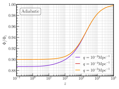
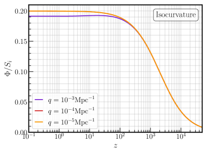
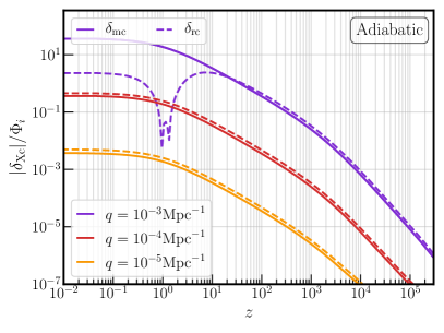
Figure 3: Transfer functions for $\Phi$, $\delta_{\rm mc}$ and $\delta_{\rm rc}$ as a function of redshift. The top row shows $\Phi(z)$ for adiabatic (left panel) and isocurvature (right panel) initial conditions — for $q=10^{-3}\,{\rm Mpc}^{-1}$ (purple), $q=10^{-4}\,{\rm Mpc}^{-1}$ (red) and $q=10^{-5}\,{\rm Mpc}^{-1}$ (orange). Note that for superhorizon modes in the isocurvature case, $\Phi=1/5S_{i}$ already at redshifts $z\lesssim 100$. For slightly subhorizon modes the curvature perturbation has decayed a little for both initial adiabatic and isocuravture perurbations. The bottom row shows the evolution of $\delta_{\rm mc}$ (solid lines) and $\delta_{\rm rc}$ (dashed lines) for adiabatic (left panel) and isocurvature (right panel) initial conditions. For superhorizon modes, the density contrast $\delta_{\rm mc}$ of CDM is suppressed at low redshift and the initial isocurvature is transferred to radiation. For slightly subhorizon modes, the density contrast in CDM grows when the mode enters the horizon. For $q=10^{-3}\,{\rm Mpc}^{-1}$, the density contrast $\delta_{\rm mc}$ is $\sim 10$ times the initial curvature $\Phi_{i}$ or isocurvature $S_{i}$ perturbation. For $q>10^{-4}\,{\rm Mpc}^{-1}$, the amplitude of the initial curvature and isocurvature perturbations are constrained by the CMB data to be $\Phi_{i}<10^{-4}$ and $S_{i}<10^{-5}$ [79].

III.2 Effect on the number count fluctuations

We proceed to study the effect of such a discrete adiabatic superhorizon mode on the galaxy number count fluctuations. If it is still superhorizon today, we can expand the curvature perturbation in powers of $\vec{q}\cdot\vec{r}$ as

$$\Phi_{\rm MD}(\vec{q}\cdot\vec{x})=\sum_{\ell=1}^{\infty}\frac{1}{\ell!}\Phi_{{\rm MD},\ell}(qr\cos\theta)^{\ell}\,,$$ (47)

where $\Phi_{{\rm MD},\ell}=9\Phi_{i,\ell}/10+S_{i,\ell}/5$, $q$ is the comoving wavenumber of the superhorizon mode and $r$ is the comoving distance to the Source and $\theta$ is the angle between the direction of $\vec{q}$ and $\vec{r}$. We then expand the number count fluctuations (28) similarly as

$$\Delta^{X}_{n}=\sum_{\ell=1}^{\infty}\frac{1}{\ell!}D^{X}_{\ell}(\cos\theta)^{\ell}\,,$$ (48)

where $X=\{\delta,x,{\rm evo}\}$. We will compute $D^{X}_{\ell}$ up to $\ell=3$. Then, we consider that

$$\Phi(a)=\Phi_{\rm MD}(\vec{q}\cdot\vec{x}){\cal T}_{\Phi}(a)\quad{\rm and}\quad v_{\rm m}(a)=\Phi_{\rm MD}(\vec{q}\cdot\vec{x}){\cal T}_{v}(a)\,,$$ (49)

where ${\cal T}_{\Phi}(a)$ and ${\cal T}_{v}(a)$ are respectively the transfer functions for $\Phi$ and $v_{\rm m}$ given by (see Eqs. (144) and (145))

$${\cal T}_{\Phi}(a) =\frac{5\Omega_{\rm m,0}}{2}\frac{{\cal H}/{\cal H}_{0}}{a^{2}}\int_{0}^{a}\frac{da_{1}}{({\cal H}(a_{1})/{\cal H}_{0})^{3}}\,,$$ (50)

$${\cal T}_{v}(a) =\frac{5\Omega_{\rm m,0}}{2}\frac{1}{a^{2}{\cal H}_{0}}\int_{0}^{a}da_{1}\frac{a-a_{1}}{a_{1}}\frac{1}{({\cal H}(a_{1})/{\cal H}_{0})^{3}}\,.$$ (51)

In a dust-dominated flat universe i.e. for $\Omega_{\rm m,0}=1$, we have

$${\cal T}^{\rm dust}_{\Phi}(a)=1\quad{\rm and}\quad{\cal T}^{\rm dust}_{v}(a)={\eta}/{3}\,.$$ (52)

Let us focus first on the effect of a superhorizon mode dipole, i.e. the $\ell=1$ component of Eq. (47), on the dipole of Eq. (48) $\Delta_{\cal N}$. Note that because of the presence of a Laplacian in $\delta_{r}$ (28), we also have a contribution to $\ell=1$ in Eq. (48) from the $\ell=3$ mode in Eq. (47). This however is of order $(qr)^{3}$, the form of which we present later. For simplicity, we start with the dust-dominated universe with the transfer functions given by Eq. (52). In this case

$$\delta\omega_{s}=\frac{2}{3}q\lambda_{s}\mu\quad ,\quad\delta\eta_{s}=q\lambda_{s}\mu\left(\frac{1}{3}\eta_{0}-\lambda_{s}\right)\quad,\quad\delta_{\rm mc}=0\,,$$

$$\delta\lambda_{s}=-\frac{2}{3}q\lambda_{s}\mu\quad ,\quad\delta_{r}=0\quad{\rm and}\quad{\cal H}_{s}v_{s}=\frac{1}{3}q\lambda_{s}\mu\,,$$ (53)

where we defined $\mu\equiv\cos\theta$ and used $r=\lambda=\eta_{0}-\eta$. Inserting Eq. (III.2) into Eq. (28) it is straightforward to check that $D^{\delta}_{1}=D^{x}_{1}=D^{{\rm evo}}_{1}={\cal O}((qr)^{3})$. This means that, in a dust-dominated universe, there is no dipole in the galaxy number count fluctuations from a dipole in an adiabatic superhorizon mode.

This result also holds for the matter+$\Lambda$ universe but to demonstrate this requires more work. First, it is more convenient to use the expressions for $\delta\eta$ (115) and $\delta_{r}$ (B) in Appendix B. Then, we insert the $\ell=1$ term of Eq. (47) into Eq. (18), Eq. (115) and Eq. (B). Using the formulae (149) and (150) we can do some of the integrals to arrive at:

$$\delta\omega_{s} =-q\mu\lambda_{s}{\cal T}_{\Phi}(a)+\frac{2}{3\Omega_{{\rm m},0}}q\mu\lambda_{s}\,,$$ (54)

$$\delta\eta_{s} =q\mu\lambda_{s}{\cal T}_{v}(1)-2q\mu\int_{0}^{\lambda_{s}}d\lambda_{1}(\lambda_{s}-\lambda_{1})q\mu{\cal T}_{\Phi}(a)\,,$$ (55)

$$\delta_{r} =q\mu\lambda_{s}{\cal T}_{\Phi}(a)+\frac{q\mu}{{\cal H}_{0}}\left[\frac{1}{a^{2}}\int_{0}^{a}da_{1}\frac{a^{2}-a_{1}^{2}}{a_{1}^{2}({\cal H}(a_{1})/{\cal H}_{0})^{3}}\right]^{a=a_{s}}_{a=1}+\frac{2}{\lambda_{s}}\int_{0}^{\lambda_{s}}d\lambda_{1}(\lambda_{s}-\lambda_{1})q\mu{\cal T}_{\Phi}(a)\,.$$ (56)

Plugging in Eqs. (54)-(56) into Eq. (28) and using the integrals (151) and (152), we find

$$D^{\delta}_{1}=D^{x}_{1}=D^{{\rm evo}}_{1}={\cal O}((qr)^{3})\,.$$ (57)

Hence there is no leading order dipole contribution to the galaxy number count fluctuations from an adiabatic superhorizon mode dipole, even in a general matter+$\Lambda$ universe.

This is similar to the case of the CMB, where no adiabatic superhorizon mode affects the CMB dipole at leading order [29]. Since the dipole in the galaxy number counts and in the CMB arise at the same order, it is thus not possible for an adiabatic superhorizon mode to explain the dipole tension. We now explore the possibility of an isocurvature superhorizon mode which can affect the CMB dipole, but not the number count dipole.

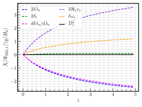
Figure 4: Different contributions to the number count dipole $D^{\delta}_{1}$ (48). Dashed lines show the different terms in $\Delta^{\delta}_{n}$ (29), which are respectively $\delta\lambda_{s}$ (blue), $\delta_{r}$ (green), $d\delta\lambda_{s}/d\lambda_{s}$ (magenta), ${\cal H}_{s}v_{s}$ (purple) and $\delta\omega_{s}$ (orange), while their sum is shown as the solid black line. Note there is an exact cancellation and $D^{\delta}_{1}=0$ at leading order for adiabatic initial conditions. Similar cancellations occur for the other contributions to the dipole, i.e. $D^{x}_{1}=0$ and $D^{\rm evo}_{1}=0$.

The contribution from higher $\ell$ terms to the dipole, quadrupole and octupole have to be computed numerically for a general matter+$\Lambda$ universe and are shown in Figs. 5. Here we present the analytical results for a matter-dominated universe. First, the contribution to $\ell=1$ is given by

$$D^{\delta}_{1}=\frac{1}{6}(q\lambda_{s})^{3}\Phi_{{\rm MD},3}\quad,\quad D^{x}_{1}=\frac{1}{12}(q\lambda_{s})^{3}\Phi_{{\rm MD},3}\quad{\rm and}\quad D^{\rm evo}_{1}=0\,.$$ (58)

Then, the contribution to the quadrupole reads

$$D^{\delta}_{2} =-(q\lambda_{s})^{2}\Phi_{{\rm MD},2}\left(\frac{1}{6}-\frac{8}{3\lambda_{s}{\cal H}_{0}}+\frac{4}{\lambda_{s}^{2}{\cal H}_{0}^{2}}\right)\,,$$ (59)

$$D^{x}_{2} =-(q\lambda_{s})^{2}\Phi_{{\rm MD},2}\left(\frac{1}{6}-\frac{5}{3\lambda_{s}{\cal H}_{0}}+\frac{4}{3\lambda_{s}^{2}{\cal H}_{0}^{2}}\right)\,,$$ (60)

$$D^{\rm evo}_{2} =2(q\lambda_{s})^{2}\Phi_{{\rm MD},2}\left(\frac{1}{6}-\frac{2}{3\lambda_{s}{\cal H}_{0}}\right)\,.$$ (61)

For the octupole we obtain

$$D^{\delta}_{3} =-(q\lambda_{s})^{3}\Phi_{{\rm MD},3}\left(1-\frac{7}{\lambda_{s}{\cal H}_{0}}+\frac{8}{\lambda_{s}^{2}{\cal H}_{0}^{2}}\right)\,,$$ (62)

$$D^{x}_{3} =-(q\lambda_{s})^{3}\Phi_{{\rm MD},3}\left(\frac{1}{2}-\frac{3}{\lambda_{s}{\cal H}_{0}}+\frac{2}{\lambda^{2}{\cal H}_{0}^{2}}\right)\,,$$ (63)

$$D^{\rm evo}_{3} =(q\lambda_{s})^{3}\Phi_{{\rm MD},3}\left(\frac{2}{3}-\frac{2}{\lambda_{s}{\cal H}_{0}}\right)\,.$$ (64)

Thus, a superhorizon mode predicts a quadrupole in the total number count:

$$Q_{\cal N} =\frac{1}{2}\frac{1}{\int_{0}^{\lambda_{s}}{\cal N}_{s}(\lambda,L)r^{2}d\lambda}\int_{0}^{\lambda_{s}}\left(D^{\delta}_{2}-2xD^{x}_{2}-f_{\rm evo}D^{\rm evo}_{2}\right){\cal N}_{s}(\lambda,L)r^{2}d\lambda\sim-\frac{2}{3}\Phi_{{\rm MD},2}\left(\frac{q}{H_{0}}\right)^{2}\,,$$ (65)

where we assumed that most of the contribution comes from $z<1$ because the quadrupole approaches a constant for $z=0$, and we used that

$$-f_{\rm evo}(z\ll 1)\simeq x(1+\alpha)+\frac{2(x-1)}{{\lambda{\cal H}}}+1-\frac{3}{2}\Omega_{\rm m,0}+\frac{1}{{\cal H}}\frac{d}{d\lambda}\ln\left(\frac{r^{2}{\cal N}_{s}}{{\cal H}}\right)\,.$$ (66)

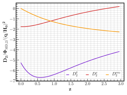
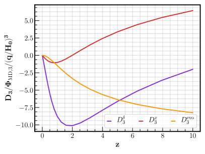
Figure 5: Evolution of the galaxy number count quadrupole (left) and octupole (right) with redshift $z$ in the matter+$\Lambda$ universe. Purple, red and orange lines show respectively the quadrupole and octupole contributions to $\Delta_{n}^{\delta}$ (29), $\Delta_{n}^{x}$ (30) and $\Delta_{n}^{x}$ (31). The fact that the quadrupole does not vanish at $z=0$ implies an anisotropy in the Hubble parameter, see § IV.

If we expand Eq. (28) in spherical harmonics instead of an expansion in powers of $(qr_{s})$, viz.

$$\Delta^{X}_{n}=\sum_{\ell=1}^{\infty}\frac{1}{\ell!}D^{X}_{\ell}(\cos\theta)^{\ell}=\sum_{\ell=1}^{\infty}a^{X}_{\ell 0}Y_{\ell 0}(\theta,\varphi)\,,$$ (67)

we have the following translation

$$a^{X}_{10}=2\sqrt{\frac{\pi}{3}}D^{X}_{1}+\frac{1}{5}\sqrt{\frac{\pi}{3}}D^{X}_{3}\quad,\quad a^{X}_{20}=\frac{2}{3}\sqrt{\frac{\pi}{5}}D^{X}_{2}\quad{\rm and}\quad a^{X}_{30}=\frac{2}{15}\sqrt{\frac{\pi}{7}}D^{X}_{3}\,.$$ (68)

$a^{X}_{10}$, $a^{X}_{20}$ and $a^{X}_{30}$ respectively are the so-called dipole, quadrupole and octupole. For the reader’s convenience we give two values of $\lambda_{s}$: $\lambda_{s}(z=2)\simeq 5300\,{\rm Mpc}$ and $\lambda_{s}(z=1)\simeq 3400\,{\rm Mpc}$.

III.3 Effect on the CMB temperature fluctuations

Now we review the effects on CMB temperature fluctuations, which in our notation reads [76]

$$\Delta^{\rm CMB}_{T}(z_{\rm dec},\hat{n})= \frac{1}{4}\delta_{\rm rc}+{\cal H}_{\rm dec}v_{\rm dec}-\delta\omega_{\rm dec}\,.$$ (69)

Note that when computing $\delta\omega_{\rm dec}$ using (18) evaluated at decoupling, we have to replace $v_{\rm m}(a_{0})$ by $v_{o}$ as it is our velocity induced by the superhorizon mode. This is not important for adiabatic modes as $v_{\rm r}=v_{\rm m}$ but it is important for isocuvature modes as there is a net relative velocity. Also since the transfer of isocurvature into curvature has not been completed at the time of decoupling, we consider both of their contributions. First, we expand for $\vec{q}\cdot\vec{r}\ll 1$ the initial curvature and isocurvature fluctuations as follows

$$\Phi_{i}(\vec{q}\cdot\vec{r})=\sum_{\ell=1}^{\infty}\frac{1}{\ell!}\Phi_{i,\ell}(qr\cos\theta)^{\ell}\quad{\rm and}\quad S_{i}(\vec{q}\cdot\vec{r})=\sum_{\ell=1}^{\infty}\frac{1}{\ell!}S_{i,\ell}(qr\cos\theta)^{\ell}\,.$$ (70)

Note that the wavenumber $q$ of the discrete modes for $\Phi$ and $S$ need not be the same; however, we chose them to be equal for simplicity. Next we take into account the corresponding transfer functions for curvature and isocurvature initial conditions by writing

$$\Phi =\Phi_{i}(\vec{q}\cdot\vec{x}){\cal T}^{\rm ad}_{\Phi}(a)+S_{i}(\vec{q}\cdot\vec{x}){\cal T}^{\rm iso}_{\Phi}(a)\,,$$ (71)

$$v_{\rm r} =\Phi_{i}(\vec{q}\cdot\vec{x}){\cal T}^{\rm ad}_{v_{\rm r}}(a)+S_{i}(\vec{q}\cdot\vec{x}){\cal T}^{\rm iso}_{v_{\rm r}}(a)\,,$$ (72)

$$\delta_{\rm rc} =S_{i}(\vec{q}\cdot\vec{x}){\cal T}^{\rm iso}_{\delta_{\rm rc}}(a)\,,$$ (73)

where the transfer functions ${\cal T}^{\rm ad/iso}_{Y}$ with $Y=\{\Phi,v_{\rm r},\delta_{\rm rc}\}$ are Eqs. (138)-(143) in Appendix II.1. Then, we do the same expansion as before but for the CMB temperature fluctuations:

$$\Delta^{\rm CMB}_{T}=\sum_{\ell=1}^{\infty}\frac{1}{\ell!}D^{\rm CMB}_{\ell}(\cos\theta)^{\ell}=\sum_{\ell=1}^{\infty}a^{\rm CMB}_{\ell 0}Y_{\ell 0}(\theta,\varphi)\,.$$ (74)

Using the expression for $\delta\omega$ (18), and evaluating at the time of decoupling, we find

$$D^{\rm CMB}_{1} \simeq-0.18(qr_{\rm dec})S_{i,1}\,,$$ (75)

$$D^{\rm CMB}_{2} \simeq-(qr_{\rm dec})^{2}\left(0.32\Phi_{i,2}+0.24S_{i,2}\right)\,,$$ (76)

$$D^{\rm CMB}_{3} \simeq-(qr_{\rm dec})^{3}\left(0.33\Phi_{i,3}+0.24S_{i,3}\right)\,.$$ (77)

We see that only the initial isocurvature may affect the CMB dipole. The integrals were done analytically. The coefficients of the adiabatic components in Eqs. (76) and (77) are in agreement with Ref. [41]. However, the coefficients of the isocurvature components are about half of those calculated in Ref. [42], the likely reason for the discrepancy being that these authors assume the MD era to begin only at CMB decoupling. Hence the curvature perturbation has only reached $\Phi\sim 0.13S_{i}$, compared to $\Phi=S_{i}/5$ for the usual longer period of matter-domination. We believe that this suppression because of an incomplete transfer from isocurvature to curvature accounts for the missing factor of $\sim 2$. For the reader’s convenience we give here the value for the comoving distance to decoupling: $r_{\rm dec}=\lambda_{\rm dec}=\eta_{0}-\eta_{\rm dec}\simeq 14100\,{\rm Mpc}$.

IV Superhorizon modes and the dipole tension

Now we can discuss the viability of superhorizon perturbations to alleviate the dipole tension. (The effects of slightly subhorizon modes are discussed in § V.) Let us first review measurements of the CMB and quasar number count dipoles. The former has been measured by Planck [24] to be

$$D^{\rm CMB}_{1}=(1.23357\pm 0.00036)\times 10^{-3}\,.$$ (78)

If it is entirely kinematic in origin, then we have a precise measurement of the velocity of the Solar system barycentre with respect to the CRF:

$$n_{i}v^{i}_{o}=369.82\pm 0.11~{}{\rm km/s}$$ (79)

Planck has also looked for the aberration and modulation effects due to the Observer’s velocity [31], obtaining

$$n_{i}v^{i}_{o}=384\pm 78\,{\rm(stat)}\pm 115\,{\rm(syst)}\,{\rm km/s},$$ (80)

which is consistent with the kinematic interpretation (79) but has a large uncertainty. Hence the relative velocity with the CRF can in principle be larger if there is also a significant intrinsic contribution to the CMB dipole. However even when such an intrinsic dipole is allowed to be non-zero, the peculiar velocity of the Solar system inferred from Planck data is $n_{i}v^{i}_{o}=300^{+111}_{-93}\,{\rm km/s}$ [35, 36]. Analysis of the dipolar spectra of the bipolar spherical harmonics of Planck data also finds consistency with the purely kinematic interpretation (79) at high significance [33].

On the other hand the quasar number count dipole is [20]

$$d_{\cal N}=(15.54\pm 1.7)\times 10^{-3}\,,$$ (81)

where the error estimate is from Ref. [77]. Since we have shown (§ III) that superhorizon modes do not induce a significant dipole in the number count, let us consider the possibility that Eq. (81) is the real kinematic dipole, due to our motion with respect to the CRF of

$$n_{i}v^{i}_{o}=(2.66\pm 0.29)\times 10^{-3}\Rightarrow 797\pm 87\,{\rm km/s}\,,$$ (82)

This is discrepant at $4.9\sigma$ with the velocity extracted from the CMB if its dipole is purely kinematic in origin. Note however that the velocity (82) is discrepant with the value (80) obtained by Planck observations of aberration and modulation at only $3\sigma$.

Figure 6: Illustration of the effects of an early CDM isocurvature mode today, in the shear-free gauge for easier comparison with the calculations in § III. We denote by $v^{i}_{\rm LG}$, $v^{i}_{\rm DM}$ and $v^{i}_{\rm CMB}$, respectively, the velocities of the Local Group, the dark matter rest frame and the CMB rest frame. From the galaxy number count dipole our velocity $v^{i}_{\odot}$ with respect to the dark matter rest frame is $n_{i}v^{i}_{\odot}\simeq 800\,{\rm km/s}$. However, the CMB rest frame moves away from the matter rest frame with $n_{i}v^{i}_{\rm rel}\simeq 800\,{\rm km/s}$, for the parameters in Eq. (84). This, together with the large density fluctuations in the photon field, leads to a CMB dipole consistent with observations. Note that the isocurvature mode needs to be aligned with the CMB dipole.

However, if Observer’s velocity is as large as Eq. (82), the CMB dipole must have a large (negative) intrinsic contribution in order to be consistent with Eq. (78). As discussed earlier in § III, a superhorizon isocurvature mode can contribute to the dipole [38, 56, 41]. Including the effects of such a mode (75) we have

$$d^{\rm CMB}=d^{\rm CMB}_{\rm kin}+D^{\rm CMB}_{1}=n_{i}v^{i}_{o}-0.18(qr_{\rm dec})S_{i,1}=1.23357\times 10^{-3}\,,$$ (83)

if we assume that the superhorizon mode is aligned with the CMB kinematic dipole, for which there is no obvious rationale. Note also that we consider a single isocurvature mode, which may be thought of as a sharp peak in the power spectrum of isocurvature fluctuations; if the spectrum were flat, we would be constrained by the effect of isocurvature on other CMB multipoles [79]. With these important assumptions, we use the mean $v_{o}$ from Eq. (82) to conclude that a superhorizon isocurvature mode with amplitude

$$(qr_{\rm dec})S_{i,1}\simeq 7.9\times 10^{-3}-0.015\left(1-\frac{n_{i}v^{i}_{o}}{797~{}{\rm km/s}}\right)\,,$$ (84)

would yield a CMB dipole compatible with observations. The values above are possible if, e.g., $q\sim 0.1/r_{\rm dec}\simeq 7\times 10^{-6}\,{\rm Mpc}^{-1}$ and $S_{i,1}\sim 0.1$. Note that while such an early isocurvature superhorizon mode may allow for a large peculiar velocity to be compatible with the CMB dipole, it does not explain why our Solar system moves at $797\,{\rm km/s}$ with respect to the CRF, nor why the isocurvature mode is aligned with the kinematic dipole. The necessary alignment would have to be accidental, however such a large local velocity with respect to the CRF may be realisable in models where scale-dependent non-Gaussianity is sufficiently enhanced at small comoving scales, but suppressed at larger scales so as to be unconstrained by CMB observations.

We now proceed to investigate the compatibility of this scenario with the CMB quadrupole and study possible connections to future observations.

IV.1 CMB quadrupole

Superhorizon modes can be constrained by measuring the CMB quadrupole [41]. Let us consider for simplicity only an early isocurvature mode, so that $\Phi_{i}=0$. Then we have from the intrinsic dipole (84) that the induced CMB quadrupole (76) is

$$D^{\rm CMB}_{2} \simeq-0.24(qr_{\rm dec})^{2}S_{i,2}\simeq-1.5\times 10^{-5}\frac{S_{i,2}}{S_{i,1}^{2}}\,.$$ (85)

Thus, assuming that $S_{i,2}\sim S_{i,1}^{2}$, as occurs for instance in curvaton models [42], we have

$$a_{20}\simeq-8\times 10^{-6}\,.$$ (86)

It is interesting that the Planck measurement [24, 78] of the quadrupole reads

$${\cal D}_{\ell=2}\simeq 2.3_{-0.9}^{+3.1}\times 10^{2}\,\mu{\rm K}^{2}\,,$$ (87)

where we followed their notation for ${\cal D}_{\ell}$ [50, 24]. This means that $a_{20}<1.3\times 10^{-5}$at $3\sigma$. For comparison the power-law $\Lambda$CDM model best fit [78] gives ${\cal D}_{\ell=2}=1016~{}\mu{\rm K}^{2}$, i.e. the observed quadrupole is much smaller than the standard model expectation. Hence not only does Eq. (86) provide a contribution within $3\sigma$ of the observed value, due to the minus sign it can potentially reconcile the larger best-fit expectation with observations. However to make a quantitative prediction, we need a concrete model for the isocurvature mode which we leave for future work.

IV.2 Anisotropy of the Hubble parameter

We briefly discuss how the superhorizon mode would also affect the luminosity distance. which in our notation (§ II) is:

$$d_{L}=\hat{d}_{o}(1+z)^{2}\,.$$ (88)

We find that the fluctuations in the luminosity distance read

$$\frac{\delta d_{L}}{d_{L}}=\Delta_{n}^{x}\,,$$ (89)

where $\Delta_{n}^{x}$ is given in Eq. (30) (see also Refs. [80, 81]). Thus we conclude from Eq. (57) that the dipole in the luminosity distance is unaffected by the superhorizon mode at leading order in $q\lambda_{s}$. However, the next-order effect would be more important for the quadrupole. Eq. (59) shows that for low redshift, that is $\lambda_{s}{\cal H}_{0}\ll 1)$, the quadrupole is approximately given by

$$D_{2}^{d_{L}}\simeq-\frac{4}{15}\left(\frac{q}{{\cal H}_{0}}\right)^{2}S_{i,2}\sim-6\times 10^{-6}\frac{S_{i,2}}{S_{i,1}^{2}}\,.$$ (90)

This constant anisotropy at $z\ll 1$ in the Hubble parameter from the quadrupole was first noted in Ref. [43]. Although small, it may be detectable in forthcoming large surveys.

V Slightly subhorizon modes and the dipole tension

In the previous section we have considered the effect of superhorizon modes on the galaxy number count fluctuations and found that, in general, no adiabatic superhorizon mode can source a number count dipole at leading order in $q\lambda$. Now we study the effects of slightly subhorizon modes, by which we mean modes which were superhorizon at the time of CMB decoupling but have wavelength much smaller than the path travelled by the photons from the Source. We thus consider wavenumbers in the range $5\times 10^{-3}\,{\rm Mpc}^{-1}>q>7\times 10^{-5}\,{\rm Mpc}^{-1}$, so that $q\eta_{\rm dec}\ll 1$ but $q\eta_{0}>q\lambda_{s}\gg 1$. Modes with larger wavenumbers, i.e. $q>5\times 10^{-3}$, contribute to the so-called clustering dipole, which has been estimated to be of ${\cal O}(10^{-4})$ for the quasar sample considered in Ref. [20].

Let us first clarify our approach. In contrast to § IV, we assume as is standard that the CMB dipole is kinematic and take $n_{i}v^{i}_{\odot}\simeq 369\,{\rm km/s}$ (79). In the general case, one should also consider the possible contribution from superhorizon modes as in § IV. Then, to be consistent with the results of Ref. [20, 21], the number count dipole must have an additional intrinsic contribution, viz.

$$d_{\cal N}=d^{\rm kin}_{\cal N}+d^{\rm int}_{\cal N}\,.$$ (91)

Using Eqs. (39), (79) and (81), we find that the intrinsic contribution should be approximately

$$d^{\rm int}_{\cal N}\simeq 9\times 10^{-3}\,.$$ (92)

For subhorizon modes $qr>1$, so we can expand directly in terms of spherical harmonics $Y_{l0}$ and spherical Bessel functions $j_{l}$:

$$\Phi=\sum_{l=0}^{\infty}\Phi_{l}(2l+1)j_{l}(qr)Y_{l0}(\theta)\,,$$ (93)

and similarly for isocurvature, density and velocity perturbations. Since we assumed that the subhorizon mode is aligned with the number count dipole, we only have the $Y_{l0}(\theta)$ contributions. The time dependence of $\Phi_{l}$ is given by the transfer functions of a radiation+matter-dominated universe. Since we are dealing with subhorizon modes, we numerically solve the Einstein equations given in Appendix C.2 and set the initial conditions deep inside the radiation-dominated universe. For purely adiabatic modes we can use the analytical solutions given in Eqs. (52) and (148). We do not include the effect of the cosmological constant $\Lambda$ which is only relevant at $z\lesssim 0.8$. In general the effect of $\Lambda$ is to suppress structure growth so the estimates below should be understood as a conservative upper bound. Also, we do not consider the effects of baryons so the final results are uncertain to $\sim 10\%$, however this does not change our conclusions.

Figure 7: Dipole contributions to the galaxy number count (28) in terms of wavenumber at redshift $z=2$, normalised to the initial amplitude $\Phi_{1}$. We see that the larger the wavenumber the more subhorizon a mode is, hence the larger the contribution to the dipole, reaching ${\cal O}(10)$ for $q\sim 10^{-3}\,{\rm Mpc}^{-1}$. The oscillations present for $q\gtrsim 10^{-3}\,{\rm Mpc}^{-1}$ are due to the Taylor expansion (93) in terms of Bessel functions.

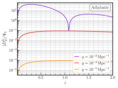
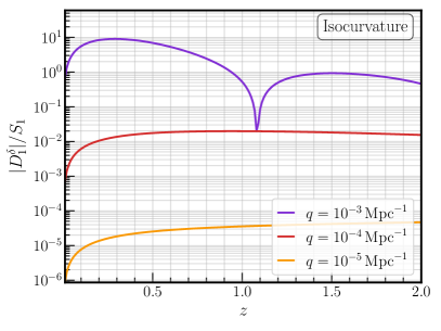
Figure 8: Contribution $D_{1}^{\delta}$(29) to the number count dipole (28) versus redshift for modes with $q=\{10^{-3}$ (purple), $10^{-4}$ (red), $10^{-5}$ (orange)$\}~{}{\rm Mpc}^{-1}$, for adiabatic (left) and isocurvature (right) initial conditions.

With the numerical solutions to the radiation+matter-dominated universe and the expansion in terms of Bessel functions (93), we compute the dipole of the number count using Eq. (28). Fig. 7 shows the dependence of the different contributions to the dipole in (28) with wavenumber $q$ for a pure adiabatic mode. We see that the larger the wavenumber, the more density fluctuations have grown and the larger the dipole. However, the larger the wavenumber, the tighter too are the CMB constraints from Planck [79]. Roughly we have that $\Phi_{i}<5.2\times 10^{-5}$ for $q\sim 10^{-3}\,{\rm Mpc}^{-1}$, where $\Phi_{i}$ is the amplitude of the primordial curvature perturbation. Isocurvature perturbations can have an amplitude of at most $10\%$ of the curvature perturbation, hence $S_{i}<10^{-5}$ for $q\sim 10^{-3}\,{\rm Mpc}^{-1}$.

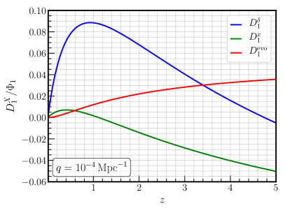
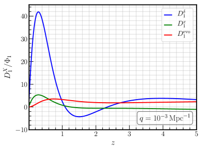
Figure 9: Contributions to the number count dipole (28) versus redshift for $q=10^{-4}{\rm Mpc}^{-1}$ (left panel) and $q=10^{-3}{\rm Mpc}^{-1}$ (right panel), both for adiabatic initial conditions. For $q=10^{-4}{\rm Mpc}^{-1}$ the largest contribution peaks at $z\sim 1$ with amplitude $D_{1}^{\delta}\sim 0.09\,\Phi_{1}$. For $q=10^{-3}{\rm Mpc}^{-1}$ the largest contribution peaks at $z\sim 0.5$ with amplitude $D_{1}^{\delta}\sim 42\,\Phi_{1}$.

In Fig. 8 we show the redshift dependence of the contribution $D_{1}^{\delta}$ (29) to the number count dipole (28) for wavenumbers $q=\{10^{-3},10^{-4},10^{-5}\}\,{\rm Mpc}^{-1}$ and for both adiabatic and isocurvature initial conditions. We see that the contribution of initial isocurvature to the number count is suppressed by nearly an order of magnitude with respect to the adiabatic case. Hence for simplicity, we proceed with slightly subhorizon adiabatic modes, which are also not as constrained by Planck [79] as isocurvature fluctuations. The contributions to the number count dipole for $q=10^{-4}{\rm Mpc}^{-1}$ and $q=10^{-3}{\rm Mpc}^{-1}$ for this case are shown in Fig. 9. For $q=10^{-4}{\rm Mpc}^{-1}$ we see that at redshifts of $z\sim 1$ the largest contribution comes from $D_{1}^{\delta}$ with an amplitude of the order of $0.09\,\Phi_{1}$. However, taking into account the above-mentioned CMB constraints [79], the dipole from $q=10^{-4}{\rm Mpc}^{-1}$ is $D_{1}^{\delta}\sim{\cal O}(10^{-5})$. For $q=10^{-3}{\rm Mpc}^{-1}$ we see that $D_{1}^{\delta}$ peaks at $z\sim 0.5$ with an amplitude $D_{1}^{\delta}\sim 42\,\Phi_{1}$. The dipole allowed by CMB constraints is then $D_{1}^{\delta}\sim{\cal O}(10^{-3})$. Note, however, that the intrinsic dipole in the total number count is given by

$$d^{\rm int}_{\cal N} =\frac{1}{\int_{0}^{\lambda_{s}}{\cal N}_{s}(\lambda,L)r^{2}d\lambda}\int_{0}^{\lambda_{s}}\left(b\,D_{1}^{\delta}-2xD_{1}^{x}-f_{\rm evo}D_{1}^{\rm evo}\right){\cal N}_{s}(\lambda,L)r^{2}d\lambda\,.$$ (94)

Although an accurate calculation requires knowledge of the evolution of the sources in redshift which is uncertain, we can obtain a rough estimate as follows. First, since for $q\sim 10^{-3}{\rm Mpc}^{-1}$, $D_{1}^{\delta}$ is by far the dominant contribution at $z<1$ and the quasar numbers also peak at $z\sim 1$, we may evaluate the integrals at this redshift. Then, taking $b=1$, this gives $d^{\rm int}_{\cal N}\sim D_{1}^{\delta}$. This implies that a discrete adiabatic mode with $q\sim 10^{-3}{\rm Mpc}^{-1}$ can yield at most $d^{\rm int}_{\cal N}\sim{\cal O}(10^{-3})$. Hence this cannot solve the dipole tension but it suggests that a collection of modes with $q\sim 10^{-3}{\rm Mpc}^{-1}$, say corresponding to a ‘bump’ in the primordial spectrum (as seen in reconstructions, e.g. Figure 2 of Ref. [82]), could add up to a sizeable contribution to the number count dipole. The above order of magnitude estimate illustrates that while slightly subhorizon modes cannot explain the number count dipole, they do deserve further study which we leave for future work.

VI Discussion & conclusions

	Adiabatic discrete mode	Isocurvature discrete mode
Superhorizon ($q<{\cal H}_{0}$)	No CMB dipole∗ [41] No NC dipole∗ Cannot solve dipole tension	Intrinsic CMB dipole [41] No NC dipole∗ Might resolve dipole tension∗∗
Slightly subhorizon (${\cal H}_{0}\lesssim q\lesssim{\cal H}_{\rm dec}$)	Amplitude $\lesssim 8\times 10^{-5}$ (CMB [79]) ${\cal O}(10^{-3})$ maximum NC dipole Cannot solve dipole tension	Amplitude $\lesssim 10\%$ of adiabatic [79] ${\cal O}(10^{-4})$ maximum NC dipole Cannot solve dipole tension
Subhorizon ($q\gtrsim{\cal H}_{\rm dec}$)	Amplitude $\sim 5\times 10^{-5}$ [79] Cannot solve dipole tension [20]	Amplitude $\lesssim 10\%$ of adiabatic [79] Cannot solve dipole tension

The recently reported mismatch between the CMB dipole [24] and the predicted quasar number count dipole [20, 21] suggests that the rest frames of the CMB and dark matter are different. We have investigated if this tension can be due to the effects of primordial fluctuations with wavelength exceeding or similar to the current Hubble radius. Our main results are summarised in Table LABEL:tab:table1.

We find that, as for the CMB dipole [41], an initial adiabatic superhorizon mode does not affect the number count dipole at leading order in $qr<1$, where $q$ is the wavenumber of the superhorizon mode and $r$ the comoving distance travelled by the photons. Next, we considered initial CDM isocurvature perturbations, which may originate in axion or curvaton models. However, since isocurvature perturbations are converted into adiabatic ones in the matter-dominated era [27], we find that there is practically no induced dipole in the number count of sources which are mainly at redshifts $z\lesssim 2$. Therefore initial CDM superhorizon isocurvature perturbations do not affect the number count dipole either. However, these can induce an intrinsic CMB dipole [29, 38, 42].

We thus argued that an isocurvature superhorizon mode with an amplitude of $\sim 0.1$ and a wavelength of $\sim 10$ times the current horizon can reconcile the quasar number count [20, 21] and the CMB dipoles [24] by allowing for a large peculiar velocity of the Solar system of about 800 km/s with respect to the CRF. The isocurvature superhorizon mode provides a negative intrinsic contribution to the CMB dipole, cancelling about half of the kinematic dipole due to our large peculiar velocity. The required amplitude is compatible with measurements of the CMB quadrupole.

While an early isocurvature superhorizon mode allows for a large peculiar velocity to be compatible with the CMB dipole, it does not explain why the intrinsic dipole should be aligned with the CMB dipole, nor why our Solar system should move at $\sim 800$ km/s with respect to the CRF. Nearby superclusters can account for up to $\sim 300\,{\rm km/s}$ of that peculiar velocity (see e.g. [83] and references therein). The remaining $\sim 500\,{\rm km/s}$ might be due to even bigger structures beyond our Local Group or due to large non-Gaussianities on small scales. We note, however, that the presence of such large inhomogeneities beyond $200/h\,{\rm Mpc}^{-1}$ is not expected in $\Lambda$CDM and may be in conflict with CMB lensing observations. Such potential ways to falsify the superhorizon scenario and the investigation of the impact of large non-Gaussianities on small scales on the local velocity dispersion are beyond the scope of this paper. But we plan to explore them in subsequent works.

As an alternative, we explored in § V the effect of slightly subhorizon modes, i.e., subhorizon today but superhorizon at decoupling, now assuming that the CMB dipole is kinematic but that there may be an intrinsic contribution to the number count dipole. First, we find that the effect of initial adiabatic fluctuations on the dipole is larger than the early isocurvature case. Second, we find that since both CDM density fluctuations and velocities of subhorizon modes grow with time, the dipole due to such fluctuations is larger at larger wavenumbers and smaller redshifts. For instance, the dipole for $q\sim 10^{-3}\,{\rm Mpc}^{-1}$ peaks at $z\sim 0.5$ with an amplitude of $\sim 40$ times the amplitude of primordial fluctuations. However, CMB measurements constrain the amplitude of the primordial fluctuations to be $\Phi_{i}<5\times 10^{-5}$. Thus, discrete slightly subhorizon adiabatic modes with $q\sim 10^{-3}\,{\rm Mpc}^{-1}$ can at most generate a dipole in the number count of ${\cal O}(10^{-3})$, which is insufficient to explain the large number count dipole [20, 21]. Nevertheless, there is the possibility that a collection of modes with $q\sim 10^{-3}\,{\rm Mpc}^{-1}$ may generate a sizeable dipole. A characteristic signal of such slightly subhorizon modes is a redshift dependent dipole with a peak at $z\sim 0.5$. We leave a detailed study of this possibility for future works.

We have neglected the effects of baryons and neutrinos, however this does not significantly affect our results. Furthermore, in the late universe baryons fall into the dark matter gravitational potential wells and therefore follow the CDM distribution. Therefore we do not expect that baryons or initial baryon isocurvature would change our conclusions concerning the galaxy number count. An interesting possibility worth studying is the effect of initial velocity isocurvature perturbations (or any process that can induce relative velocities), although it is not clear how such perturbations can be generated in the early universe. Moreover for simplicity we focused on a single discrete CDM isocurvature mode. Hence our analysis should apply to isocurvature perturbations with a sharp peak in their primordial spectrum, but further work is required for a broad featureless spectrum. Also we have not presented any concrete model that can generate such isocurvature modes. The simplest assumption is that these are remnants of the pre-inflationary universe [56, 58, 59, 60, 61]. It would be interesting also to consider the above scenario in axion isocurvature models.

The superhorizon isocurvature scenario proposed in this work to resolve the dipole tension will be tested by future experiments. First, proposed future CMB experiments [89] and new techniques [90, 91] will test the kinematic hypothesis more precisely. For instance, a (non)-detection of a CMB intrinsic component of ${\cal O}(10^{-3})$ could (rule out) hint towards an isocurvature superhorizon mode; for recent work in this direction see [35, 36]. Also, an intrinsic CMB dipole component implies a frequency dependence of the CMB quadrupole [92]. Second, information on the redshift dependence of the number count dipole as well as possibly the number count quadrupole will come from the Legacy Survey of Space & Time (LSST) by the Rubin Observatory [93], as well the Square Kilometre Array (SKA) [94]. The isocurvature superhorizon mode scenario implies a constant (purely kinematic) dipole in the galaxy number count, and a quadrupole which is redshift dependent but approaches a constant today. The quadrupole in the total number count due to the superhorizon mode is predicted to be of ${\cal O}(10^{-6})$. Such a quadrupole (90) would also appear in the Hubble parameter [43] although this would be hard to detect.

The nature of the dipole may also be probed by other observations, such as the cosmic infrared background [95, 96], CMB spectral distortions [97], the stochastic gravitational wave background [98, 99, 100] and the 21-cm line [101]. It would also be interesting to perform a general joint analysis of CMB and the number counts dipole, without making any kinematic assumption.

We conclude by noting that the inference of a Cosmological Constant $\Lambda$ from late-universe observations assumes that galaxies are isotropically distributed in the reference frame in which the CMB is isotropic. Since this is apparently not the case with $>5\sigma$ significance [20, 21], even if the dipole tension is resolved in a FLRW framework with superhorizon fluctuations as we have discussed, it poses a serious challenge to the standard $\Lambda$CDM cosmology.

Appendix A Perturbative expansion in the number count

In this Appendix we provide the details necessary to follow the calculations in § II.

A.1 Photon’s geodesics

After expansion of Eq. (6), the perturbed photon’s geodesic is given by

$$\frac{d\delta k^{\mu}}{d\bar{\lambda}}=-\delta\Gamma_{\alpha\beta}^{\mu}k^{\alpha}k^{\beta}\,,$$ (95)

where

$$\delta\Gamma_{\mu\nu}^{\alpha}=2\delta^{\alpha}_{0}\delta^{0}_{(\mu}\partial_{\nu)}\Psi+2\delta^{i}_{(\mu}\partial_{\nu)}\Phi\delta^{\alpha}_{i}+\eta^{\alpha\lambda}\partial_{\lambda}\Psi\delta^{0}_{(\mu}\delta^{0}_{\nu)}-\eta^{\alpha\lambda}\partial_{\lambda}\Phi\delta^{i}_{(\mu}\delta^{j}_{\nu)}\delta_{ij}\,.$$ (96)

Contracting with the null vectors, we arrive at

$$\frac{d\delta k^{0}}{d\lambda}=2\frac{d\Psi}{d\lambda}+\frac{\partial}{\partial\eta}(\Psi-\Phi)\,,$$ (97)

and

$$\frac{d\delta k^{i}}{d\lambda}=-2n^{i}\frac{d\Phi}{d\lambda}-\partial^{i}(\Psi-\Phi)\,.$$ (98)

A.2 Observer’s area distance

Here we solve the equations for the Observer’s area distance $\tilde{d}_{0}$ using (7) and (8). First, we have that in the background

$$\theta=\partial_{i}n^{i}=\frac{2}{r(\lambda)}\quad{\rm and}\quad r(\lambda)=\lambda.$$ (99)

since $n^{i}$ is a vector in the radial direction $r$ from us. The latter equality holds in a flat FLRW model [43]. Then, at first-order we consider the variables $\tilde{d}_{o}=r(1+\delta_{r})$ and $\tilde{\theta}=2/r(1+\delta_{\theta})$, with which Eqs. (7) and (8) become

$$\frac{d}{d\lambda}\delta_{r} =\frac{1}{r(\lambda)}\delta_{\theta}\,,$$ (100)

$$\frac{d}{d\lambda}\left(r(\lambda)\delta_{\theta}\right) =-\frac{r^{2}(\lambda)}{2}\tilde{R}_{\mu\nu}k^{\mu}k^{\nu}\,.$$ (101)

We have also used that since $\tilde{\sigma}_{\mu\nu}\tilde{\sigma}^{\mu\nu}=\tilde{\nabla}_{\mu}\tilde{k}^{\nu}\tilde{\nabla}_{\nu}\tilde{k}^{\mu}-\tilde{\theta}^{2}/2$, at the background level we have $\sigma_{\mu\nu}\sigma^{\mu\nu}=0$. This implies that $\sigma_{\mu\nu}$ starts at first-order in perturbation theory and that $\sigma_{\mu\nu}\sigma^{\mu\nu}$ is a second-order quantity. After integration of Eqs. (100) and (101) we find

$$\delta_{r}(\lambda_{s})=\delta_{r}(0)-\frac{1}{2}\int_{0}^{\lambda_{s}}\frac{d\lambda_{1}}{r^{2}(\lambda_{1})}\int_{0}^{\lambda_{1}}d\lambda_{2}\,r^{2}(\lambda_{2})\tilde{R}_{\mu\nu}k^{\mu}k^{\nu}\,.$$ (102)

Expanding the Ricci tensor at linear order in perturbation theory, we obtain

$$\tilde{R}_{\mu\nu}k^{\mu}k^{\nu}=\partial_{\alpha}\partial^{\alpha}\left(\Psi-\Phi\right)-2\frac{d}{d\lambda}\frac{\partial\Psi}{\partial\eta}+2\frac{d}{d\lambda}n^{i}\partial_{i}\Phi-\frac{d^{2}}{d\lambda^{2}}\left(\Psi+3\Phi\right)\,,$$ (103)

where we used that at leading order $dn^{i}/d\lambda=0$. In the above equation, we used that in cartesian coordinates $\tilde{\Gamma}_{\mu\nu}^{\alpha}$ is a first-order quantity and therefore at leading order

$$\tilde{R}_{\mu\nu}=\partial_{\alpha}\tilde{\Gamma}_{\mu\nu}^{\alpha}-\partial_{\mu}\partial_{\nu}\ln\sqrt{-\tilde{g}}$$ (104)

Then we also used that

$$\partial_{\mu}\partial_{\nu}\ln\sqrt{-\tilde{g}}=\tilde{\nabla}_{\mu}\tilde{\nabla}_{\nu}\ln\sqrt{-\tilde{g}}+\tilde{\Gamma}_{\mu\nu}^{\alpha}\tilde{\nabla}_{\alpha}\ln\sqrt{-\tilde{g}}$$ (105)

so that at leading order

$$\tilde{k}^{\mu}\tilde{k}^{\nu}\tilde{\nabla}_{\mu}\tilde{\nabla}_{\nu}\ln\sqrt{-\tilde{g}}=\tilde{k}^{\mu}\tilde{\nabla}_{\mu}(\tilde{k}^{\nu}\tilde{\nabla}_{\nu}\ln\sqrt{-\tilde{g}})-\tilde{k}^{\mu}\tilde{\nabla}_{\mu}\tilde{k}^{\nu}\tilde{\nabla}_{\nu}\ln\sqrt{-\tilde{g}}=\frac{d^{2}}{d\lambda^{2}}\ln\sqrt{-\tilde{g}}\,,$$ (106)

where we used the geodesic equation $\tilde{k}^{\mu}\tilde{\nabla}_{\mu}\tilde{k}^{\nu}=0$. After some simplification, we can write Eq. (103) as

$$\tilde{R}_{\mu\nu}k^{\mu}k^{\nu}=-\frac{1}{r^{2}}\Delta_{\Omega}(\Psi-\Phi)+\frac{d^{2}}{d\lambda_{2}^{2}}\Phi-\frac{2}{r}\partial_{r}(\Psi-\Phi)\,.$$ (107)

A.3 Redshift

Here we provide details on the calculation of $\delta\lambda_{s}$ to derive the $N-z$ relation. We start with the energy of the photon at a given $\bar{\lambda}$ and $\hat{n}$, which is given by

$$\hat{\omega}=(-\hat{k}_{\mu}\hat{u}^{\mu})=a^{-1}(\tilde{\eta})(\tilde{k}_{\mu}\tilde{u}^{\mu})=a^{-1}(\eta)(1+\Psi+n_{i}v^{i}-\delta k^{0}-{\cal H}\delta\eta)\,.$$ (108)

However, we observe at a fixed redshift, not at a fixed affine parameter. So let us consider $\lambda=\lambda_{s}+\delta\lambda_{s}$ where $\lambda_{s}=\eta_{o}-\eta_{s}$. Then

$$1+\tilde{z}(\lambda_{s}+\delta\lambda_{s})=1+z(\lambda_{s})=\frac{a(\eta(0))}{a(\eta(\lambda_{s}))}\,.$$ (109)

Expanding, we find that

$$1+\tilde{z}(\lambda_{s})=1+z(\lambda_{s}-\delta\lambda_{s})=1+z(\lambda_{s})-\frac{\partial z}{\partial\lambda_{s}}\delta\lambda_{s}\,.$$ (110)

Solving for $\delta\lambda_{s}$, we obtain

$$\delta\lambda_{s}=\frac{1}{{\cal H}(\lambda_{s})}\big{[}{\cal H}\delta\eta-\delta\omega\big{]}_{0}^{\lambda_{s}}\,,$$ (111)

where we integrated Eq. (97) once and then twice, which yields

$$\delta k^{0}(\lambda_{s})=\delta k^{0}(0)+2\left(\Psi(\lambda_{s})-\Psi(0)\right)+\int_{0}^{\lambda_{s}}d\lambda\frac{\partial}{\partial\eta}(\Psi-\Phi)\,.$$ (112)

and

$$\delta\eta=\int_{0}^{\lambda_{s}}d\lambda\,\delta k^{0}(\lambda,\hat{n})\,.$$ (113)

We set the conditions at the Observer position by requiring that $\delta\omega(\lambda\to 0)\to 0$ and $\delta_{r}(\lambda\to 0)$, i.e. we do not see any change if we are on top of the Source. By doing so, we have:

$$\delta k^{0}(0)=\Psi(0)+n_{i}v^{i}_{o}\quad{\rm and}\quad\delta_{r}(0)=\Phi(0)\,.$$ (114)

With these two last equalities, our calculation provides the galaxy number count including dipole and monopole contributions at the Observer.

Appendix B Comparison with other works

In this Appendix we show that our formula (28) is equivalent to that of Refs. [45, 46]. First, we rewrite Eqs. (19) and (II.1) after doing integration by parts as

$$\delta\eta =\lambda n_{i}v^{i}_{o}+\int_{0}^{\lambda}d\lambda_{1}\left(\Psi+\Phi-\Psi_{o}\right)+\int_{0}^{\lambda}d\lambda_{1}(r(\lambda)-r(\lambda_{1}))n^{i}\partial_{i}(\Psi-\Phi)\,,$$ (115)

and

$$\delta_{r}(\lambda)=\Phi_{o}+\Phi -\frac{2}{r(\lambda)}\int_{0}^{\lambda}d\lambda_{1}\Phi-\frac{1}{2r(\lambda)}\int_{0}^{\lambda}d\lambda_{1}\frac{r(\lambda)-r(\lambda_{1})}{r(\lambda_{1})}\Delta_{\Omega}(\Psi-\Phi)$$

$$-\frac{1}{r(\lambda)}\int_{0}^{\lambda}d\lambda_{1}(r(\lambda)-r(\lambda_{1}))n^{i}\partial_{i}(\Psi-\Phi)\,,$$ (116)

where $\Delta_{\Omega}$ is the Laplacian in the 2-sphere, namely

$$\Delta_{\Omega}=\frac{1}{\sin\theta}\partial_{\theta}(\sin\theta\partial_{\theta})+\frac{1}{\sin^{2}\theta}\partial_{\varphi}^{2}\,.$$ (117)

Now, plugging Eqs. (18), (20), (115) and (B) into Eq. (28), and after some lengthy algebra, we arrive at

$$\Delta_{{\cal N}}(z_{s},\hat{n})= \left(2+\frac{{\cal H}^{\prime}_{s}}{{\cal H}_{s}^{2}}+\frac{2-5s}{r_{s}{\cal H}_{s}}-f_{\rm evo}\right)n_{i}v^{i}_{o}$$

$$+b(z)\delta_{n,{\rm c}}+(3-f_{\rm evo}){\cal H}_{s}v_{s}+\Psi_{s}+n_{i}v^{i}_{s}+\frac{1}{{\cal H}_{s}}\left(\frac{d\Psi_{s}}{d\lambda_{s}}-\frac{d}{d\lambda_{s}}(n_{i}v^{i}_{s})+\Psi_{s}^{\prime}-\Phi_{s}^{\prime}\right)$$

$$+\left(5s+\frac{2-5s}{r_{s}{\cal H}_{s}}+\frac{{\cal H}^{\prime}_{s}}{{\cal H}_{s}^{2}}-f_{\rm evo}\right)\left(\Psi_{s}-n_{i}v_{s}^{i}+\int_{0}^{\lambda_{s}}d\lambda\frac{\partial}{\partial\eta}(\Psi-\Phi)\right)$$

$$+\left(2-5s\right)\Phi_{s}-\frac{2-5s}{2r_{s}}\int_{0}^{\lambda_{s}}d\lambda\frac{r_{s}-r}{r}\Delta_{\Omega}(\Psi-\Phi)+\frac{2-5s}{r_{s}}\int_{0}^{\lambda_{s}}d\lambda(\Psi-\Phi)\,,$$ (118)

where we dropped the monopole terms, and have defined

$$s(z)\equiv-\frac{2}{5}\frac{\partial\ln{\cal N}_{s}}{\partial\ln L}\quad{\rm and}\quad f_{\rm evo}\equiv-\frac{\partial\ln{\cal N}_{s}}{\partial\ln(1+z_{s})}\,.$$ (119)

Eq. (B) coincides exactly with that given by Challinor & Lewis [46] and Bonvin & Durrer [45] (see also Ref. [22]). A useful text for such calculations is the one by Durrer [76].

Appendix C Einstein equations

In this Appendix, we write for completeness the Einstein equations used in the main text. We take the metric to be given by

$$d\hat{s}^{2}=a^{2}(\eta)\left(-(1+2\Psi)d\eta^{2}+(1+2\Phi)\delta_{ij}dx^{i}dx^{j}\right)\,.$$ (120)

We consider an energy-momentum tensor that includes radiation $\rm r$, pressureless matter $\rm m$ and a cosmological constant $\Lambda$ with

$$T^{X}_{\mu\nu}=(\rho_{X}+P_{X})\hat{u}_{X\mu}\hat{u}_{X\nu}+P_{X}g_{\mu\nu}\,,$$ (121)

where $X=\{{\rm r},{\rm m},\Lambda\}$. We then have that $w_{X}\equiv P_{X}/\rho_{X}$ is given by $w_{\rm r}=1/3$, $w_{\rm m}=0$, $w_{\Lambda}=-1$.

C.1 Background

At the background level we have the FL equations which read

$$3M_{\rm pl}^{2}{\cal H}^{2}=a^{2}\sum_{X}\rho_{X}\,,$$ (122)

$$2M_{\rm pl}^{2}({\cal H}^{2}-2{\cal H}^{\prime})=a^{2}\sum_{X}\rho_{X}(1+w_{X})\,,$$ (123)

where a prime denotes derivative w.r.t. conformal time, i.e. ${\cal H}^{\prime}=\partial H/\partial\eta$. Energy conservation, i.e. $\rho_{X}^{\prime}+3{\cal H}(1+w_{X})\rho_{X}=0$, then yields $\rho_{\rm m}\propto a^{-3}$ and $\rho_{\rm r}\propto a^{-4}$. For convenience, we define the energy density ratios as

$$\Omega_{X}\equiv\frac{a^{2}\rho_{X}}{3M_{\rm pl}^{2}{\cal H}^{2}}\,.$$ (124)

There are analytical solutions available when $\Lambda=0$ and $\rho_{r}=0$ which are presented below. We set $a_{0}=1$ in what follows.

Radiation+matter universe:

The solution to the background equations is:

$$\frac{a(\eta)}{a_{\rm eq}}=2\left(\frac{\eta}{\eta_{*}}\right)+\left(\frac{\eta}{\eta_{*}}\right)^{2}$$ (125)

where $(\sqrt{2}-1)\eta_{*}=\eta_{\rm eq}$ and the subscript “eq” refers to the epoch of radiation-matter equality.

Matter+$\Lambda$ universe:

First, the Hubble parameter is given by

$${\cal H}={\cal H}_{0}\,a\sqrt{\Omega_{\Lambda,0}+\Omega_{{\rm m},0}a^{-3}}\,.$$ (126)

The conformal time can be written in terms of Hypergeometric functions $F[a,b,c,x]$ as

$$\eta=\int_{0}^{a}\frac{da_{1}}{a_{1}}\frac{1}{{\cal H}(a_{1})}=\frac{2\sqrt{a}}{{\cal H}_{0}\sqrt{\Omega_{{\rm m},0}}}\,F\left[\tfrac{1}{6},\tfrac{1}{2},\tfrac{7}{6},-\frac{a^{3}\Omega_{\Lambda,0}}{\Omega_{{\rm m},0}}\right]\,,$$ (127)

In this case, we have an implicit equation for $a(\eta)$.

C.2 Perturbations

To study superhorizon perturbations it is convenient to define the isocurvature perturbation and the relative velocity:

$$S\equiv\frac{\delta\rho_{\rm m}}{\rho_{\rm m}}-\frac{3}{4}\frac{\delta\rho_{\rm r}}{\rho_{\rm r}}\quad{\rm and}\quad v_{\rm rel}\equiv v_{\rm m}-v_{\rm r}\,.$$ (128)

With these variables, the linear equations for cosmological perturbations, in Fourier modes, reads:

$$\Phi^{\prime\prime}+3{\cal H}(1+c_{s}^{2})\Phi^{\prime}+({\cal H}^{2}(1+3c_{s}^{2})+2{\cal H}^{\prime})\Phi+c_{s}^{2}k^{2}\Phi=\frac{a^{2}}{2}\rho_{\rm m}c_{s}^{2}S\,,$$ (129)

and

$$S^{\prime\prime} +3{\cal H}c_{s}^{2}S^{\prime}-\frac{3}{2a^{2}\rho_{\rm r}}c_{s}^{2}{k^{4}\Phi}+\frac{3\rho_{\rm m}}{4\rho_{\rm r}}c_{s}^{2}k^{2}S=0\,,$$ (130)

where we also defined

$$c_{s}^{2}\equiv\frac{4}{9}\frac{\rho_{\rm r}}{\rho_{\rm m}+4\rho_{\rm r}/3}\,.$$ (131)

Once a solution for $\Phi$ and $S$ is found, the relative velocity is given by $v_{\rm rel}=S^{\prime}/k^{2}$. However, for superhorizon modes, it is more convenient to solve the differential equation for $v_{\rm rel}$ which reads

$$v^{\prime}_{\rm rel} +3c_{s}^{2}{\cal H}v_{\rm rel}+\frac{3}{2a^{2}\rho_{r}}c_{s}^{2}{\Delta\Phi}+\frac{3\rho_{m}}{4\rho_{r}}c_{s}^{2}S=0\,.$$ (132)

It is also useful to present the 00-component of Einstein’s equations, which is given by

$$6{\cal H}\Phi^{\prime}+6{\cal H}^{2}\Phi-2\Delta\Phi=a^{2}(\delta\rho_{\rm m}+\delta\rho_{\rm r})\,.$$ (133)

With the solutions to $\Phi$, $S$ and $v_{\rm rel}$, we can follow the evolution of the fluctuations in the matter and radiation energy densities and velocities. With the definitions (see § C.2) of $\delta_{{\rm m}c}$, $\delta_{{\rm r}c}$, $v_{{\rm m}}$ and $v_{{\rm r}}$, we have that they obey

$$\delta_{{\rm m}c}^{\prime}+\Delta v_{\rm m}-2a^{2}\rho_{\rm r}v_{\rm rel}=0\,,$$ (134)

$$\delta_{{\rm r}c}^{\prime}-{\cal H}\delta_{{\rm r}c}+\frac{4}{3}\Delta v_{\rm r}+2a^{2}\rho_{\rm m}v_{\rm rel}=0\,,$$ (135)

$$v_{\rm m}^{\prime}+{\cal H}v_{\rm m}-\Phi=0\,,$$ (136)

$$v_{\rm r}^{\prime}+{\cal H}v_{\rm r}+\frac{1}{4}\delta_{{\rm r}c}-\Phi=0\,.$$ (137)

We present the analytical solutions below.

Radiation+matter universe:

Here we only focus on superhorizon modes, namely $k\ll{\cal H}$, and so we neglect any $k$ dependence in the equations for perturbations. We may set $\Lambda=0$ as it is negligible at high redshifts. We take as initial conditions $\Phi(a\ll a_{\rm eq})=\Phi_{i}$ and $S(a\ll a_{\rm eq})=S_{i}$ and define $\xi\equiv a/a_{\rm eq}$. Then, the solutions for $k\to 0$ of (129), (130) and (132) are given by

$$S(\xi)= S_{i}\,,$$ (138)

$$\Phi(\xi)= \Phi_{i}\left(\frac{8}{5\xi^{3}}\left(\sqrt{1+\xi}-1\right)-\frac{4}{5\xi^{2}}+\frac{1}{5\xi}+\frac{9}{10}\right)$$

$$+S_{i}\left(\frac{16}{5\xi^{3}}\left(1-\sqrt{1+\xi}\right)+\frac{8}{5\xi^{2}}-\frac{2}{5\xi}+\frac{1}{5}\right)\,,$$ (139)

$$v_{\rm rel}(\xi) =S_{i}\frac{2\sqrt{2}}{3\xi{\cal H}_{\rm eq}}\left(\xi\left(3-\sqrt{1+\xi}\right)+4\left(1-\sqrt{1+\xi}\right)\right)\,.$$ (140)

Integrating (136) and (134) we arrive at

$$v_{\rm m}(\xi)= \sqrt{2}\frac{\Phi_{i}}{5{\cal H}_{\rm eq}}\left(3\sqrt{\xi+1}-\frac{4}{\xi}\frac{\xi-1+\sqrt{1+\xi}}{1+\sqrt{1+\xi}}\right)$$

$$+2\sqrt{2}\frac{S_{i}}{15{\cal H}_{\rm eq}}\left(\sqrt{1+\xi}-\frac{4}{\xi}\frac{2\xi+3-3\sqrt{1+\xi}}{1+\sqrt{1+\xi}}\right)\,,$$ (141)

$$\delta_{\rm mc}(\xi)= S_{i}+S_{i}\frac{\left(8-\sqrt{1+\xi}+4\xi-\xi^{2}\right)}{\xi^{2}}\,.$$ (142)

Lastly, we have:

$$v_{\rm r}(\xi)=v_{\rm m}(\xi)-v_{\rm rel}(\xi)\quad{\rm and}\quad\delta_{\rm rc}(\xi)=\frac{4}{3}\left(\delta_{\rm mc}(\xi)-S_{i}\right)\,.$$ (143)

Matter+$\Lambda$ universe:

Here we are interested in low enough redshift such that radiation does not play any important role. Then, the solution to Eq. (129) is [41]

$$\Phi(a)=A\frac{{\cal H}/{\cal H}_{0}}{a^{2}}\int_{0}^{a}\frac{da_{1}}{({\cal H}(a_{1})/{\cal H}_{0})^{3}}\quad{\rm with}\quad A=\frac{5}{2}\Omega_{{\rm m},0}\Phi_{\rm MD}\,,$$ (144)

so that the initial conditions are given by $\Phi(a\ll 1)=\Phi_{\rm MD}$. With the solution for $\Phi$ and the first integral of (136) we find

$$v(a)=\frac{1}{a}\int_{0}^{a}da_{1}\frac{\Phi(a_{1})}{{\cal H}(a_{1})}=\frac{A}{a^{2}{\cal H}_{0}}\int_{0}^{a}da_{1}\frac{a-a_{1}}{a_{1}}\frac{1}{({\cal H}(a_{1})/{\cal H}_{0})^{3}}\,.$$ (145)

where in the second step we used integration by parts as in Appendix D. Both integrals may be written in terms of hypergeometric functions as

$$\Phi(a)=\Phi_{q,\rm MD}F\left[\tfrac{1}{3},1,\tfrac{11}{6},-a^{3}\frac{\Omega_{\Lambda,0}}{\Omega_{{\rm m},0}}\right]\,.$$ (146)

and

$$v(a)=\frac{\Phi_{q,\rm MD}}{3{\cal H}}\left(5-3F\left[\tfrac{1}{3},1,\tfrac{11}{6},-a^{3}\frac{\Omega_{\Lambda,0}}{\Omega_{{\rm m},0}}\right]\right)\,.$$ (147)

The density fluctuations of CDM start at leading order in $q^{2}$ and are found from (135) to be given by

$$\delta_{{\rm m}c}=q^{2}\int_{0}^{a}\frac{da}{a{\cal H}}v_{\rm m}(a)\,.$$ (148)

Some useful relations are for the calculations of the dipole are:

$$\int_{0}^{\lambda}d\lambda_{1}\,\lambda_{1}\Phi^{\prime}(a_{1})=-\lambda\Phi(a)+\int_{0}^{\lambda}d\lambda_{1}\Phi(a_{1})\,,$$ (149)

$$\int_{0}^{\lambda}d\lambda_{1}\Phi(a)=-\frac{1}{2a^{2}{\cal H}_{0}}\int_{0}^{a}da_{1}\frac{a^{2}-a_{1}^{2}}{a_{1}^{2}}\frac{1}{({\cal H}(a_{1})/{\cal H}_{0})^{3}}+\frac{1}{2{\cal H}_{0}}\int_{0}^{1}da_{1}\frac{1-a_{1}^{2}}{a_{1}^{2}}\frac{1}{({\cal H}(a_{1})/{\cal H}_{0})^{3}}\,,$$ (150)

$$\int_{0}^{a}\frac{da_{1}}{a_{1}^{2}({\cal H}(a_{1})/{\cal H}_{0})^{3}}=\frac{2{\cal H}_{0}}{3\Omega_{{\rm m},0}}\left(\frac{1}{{\cal H}}+\eta\right)\,,$$ (151)

$$\int_{0}^{a}\frac{da_{1}}{a_{1}({\cal H}(a_{1})/{\cal H}_{0})^{3}}=\frac{2a{\cal H}_{0}}{3\Omega_{{\rm m},0}{\cal H}(a)}\,.$$ (152)

Appendix D Useful formulas

We convert some double definite integrals that appear in our calculations in the main text into single definite integrals by using

$$\frac{d}{d\lambda_{1}}\left(\int_{0}^{\lambda_{1}}d\lambda_{2}({\lambda_{1}-\lambda_{2}})Q(\lambda_{2})\right)=\int_{0}^{\lambda_{1}}d\lambda_{2}\,Q(\lambda_{2})\,,$$ (153)

$$\frac{d}{d\lambda_{1}}\left(\frac{1}{\lambda_{1}}\int_{0}^{\lambda_{1}}d\lambda_{2}\frac{\lambda_{1}-\lambda_{2}}{\lambda_{2}}Q(\lambda_{2})\right)=\frac{1}{\lambda_{1}^{2}}\int_{0}^{\lambda_{1}}d\lambda_{2}\,Q(\lambda_{2})\,,$$ (154)

$$\frac{d}{d\lambda_{1}}\left(\frac{1}{\lambda_{1}}\int_{0}^{\lambda_{1}}d\lambda_{2}(\lambda_{1}-\lambda_{2})Q(\lambda_{2})\right)=\frac{1}{\lambda_{1}^{2}}\int_{0}^{\lambda_{1}}d\lambda_{2}\lambda_{2}\,Q(\lambda_{2})\,,$$ (155)

$$\frac{d}{d\lambda_{1}}\left(\frac{1}{\lambda_{1}}\int_{0}^{\lambda_{1}}d\lambda_{2}(\lambda_{1}-\lambda_{2})\lambda_{2}Q(\lambda_{2})\right)=\frac{1}{\lambda_{1}^{2}}\int_{0}^{\lambda_{1}}d\lambda_{2}\lambda_{2}^{2}\,Q(\lambda_{2})\,,$$ (156)

where $Q$ may be any variable. For example, we have that after some integration by parts,

$$\int_{0}^{\lambda}\frac{d\lambda_{1}}{\lambda_{1}^{2}}\int_{0}^{\lambda_{1}}d{\lambda_{2}}\,\lambda_{2}^{2}\frac{d^{2}}{d\lambda_{2}^{2}}\Phi(\lambda_{2})=\Phi(\lambda)-\frac{2}{\lambda}\int_{0}^{\lambda_{s}}{d\lambda_{1}}\Phi(\lambda_{1})\,.$$ (157)

References

- Ellis and Baldwin [1984] G. F. R. Ellis and J. E. Baldwin, On the expected anisotropy of radio source counts, Monthly Notices of the Royal Astronomical Society 206, 377 (1984).
- Sciama [1967] D. W. Sciama, Peculiar Velocity of the Sun and the Cosmic Microwave Background, Phys. Rev. Lett. 18, 1065 (1967).
- Condon et al. [1998] J. J. Condon, W. D. Cotton, E. W. Greisen, Q. F. Yin, R. A. Perley, G. B. Taylor, and J. J. Broderick, The NRAO VLA Sky survey, Astron. J. 115, 1693 (1998).
- Mauch et al. [2003] T. Mauch, T. Murphy, H. J. Buttery, J. Curran, R. W. Hunstead, B. Piestrzynski, J. G. Robertson, and E. M. Sadler, SUMSS: A wide-field radio imaging survey of the southern sky. 2. The Source catalogue, Mon. Not. Roy. Astron. Soc. 342, 1117 (2003), arXiv:astro-ph/0303188 .
- Intema et al. [2017] H. T. Intema, P. Jagannathan, K. P. Mooley, and D. A. Frail, The GMRT 150 MHz All-sky Radio Survey: First Alternative Data Release TGSS ADR1, Astron. Astrophys. 598, A78 (2017), arXiv:1603.04368 [astro-ph.CO] .
- Eisenhardt et al. [2020] P. R. M. Eisenhardt et al., The CatWISE Preliminary Catalog: Motions from WISE and NEOWISE Data, Astrophys. J. Suppl. 247, 69 (2020), arXiv:1908.08902 [astro-ph.IM] .
- Lacy et al. [2020] M. Lacy et al., The Karl G. Jansky Very Large Array Sky Survey (VLASS). Science case and survey design, Publ. Astron. Soc. Pac. 132, 035001 (2020), arXiv:1907.01981 [astro-ph.IM] .
- McConnell et al. [2020] D. McConnell et al., The Rapid ASKAP Continuum Survey I: Design and first results, Publ. Astron. Soc. Austral. 37, e048 (2020), arXiv:2012.00747 [astro-ph.IM] .
- Blake and Wall [2002] C. Blake and J. Wall, Detection of the velocity dipole in the radio galaxies of the nrao vla sky survey, Nature 416, 150 (2002), arXiv:astro-ph/0203385 .
- Singal [2011] A. K. Singal, Large peculiar motion of the solar system from the dipole anisotropy in sky brightness due to distant radio sources, Astrophys. J. Lett. 742, L23 (2011), arXiv:1110.6260 [astro-ph.CO] .
- Gibelyou and Huterer [2012] C. Gibelyou and D. Huterer, Dipoles in the Sky, Mon. Not. Roy. Astron. Soc. 427, 1994 (2012), arXiv:1205.6476 [astro-ph.CO] .
- Rubart and Schwarz [2013] M. Rubart and D. J. Schwarz, Cosmic radio dipole from NVSS and WENSS, Astron. Astrophys. 555, A117 (2013), arXiv:1301.5559 [astro-ph.CO] .
- Tiwari et al. [2014] P. Tiwari, R. Kothari, A. Naskar, S. Nadkarni-Ghosh, and P. Jain, Dipole anisotropy in sky brightness and source count distribution in radio NVSS data, Astropart. Phys. 61, 1 (2014), arXiv:1307.1947 [astro-ph.CO] .
- Tiwari and Jain [2015] P. Tiwari and P. Jain, Dipole Anisotropy in Integrated Linearly Polarized Flux Density in NVSS Data, Mon. Not. Roy. Astron. Soc. 447, 2658 (2015), arXiv:1308.3970 [astro-ph.CO] .
- Tiwari and Nusser [2016] P. Tiwari and A. Nusser, Revisiting the NVSS number count dipole, JCAP 03, 062, arXiv:1509.02532 [astro-ph.CO] .
- Colin et al. [2017] J. Colin, R. Mohayaee, M. Rameez, and S. Sarkar, High redshift radio galaxies and divergence from the CMB dipole, Mon. Not. Roy. Astron. Soc. 471, 1045 (2017), arXiv:1703.09376 [astro-ph.CO] .
- Bengaly et al. [2018] C. A. P. Bengaly, R. Maartens, and M. G. Santos, Probing the Cosmological Principle in the counts of radio galaxies at different frequencies, JCAP 04, 031, arXiv:1710.08804 [astro-ph.CO] .
- Singal [2019] A. K. Singal, Large disparity in cosmic reference frames determined from the sky distributions of radio sources and the microwave background radiation, Phys. Rev. D 100, 063501 (2019), arXiv:1904.11362 [physics.gen-ph] .
- Siewert et al. [2021] T. M. Siewert, M. Schmidt-Rubart, and D. J. Schwarz, Cosmic radio dipole: Estimators and frequency dependence, Astron. Astrophys. 653, A9 (2021), arXiv:2010.08366 [astro-ph.CO] .
- Secrest et al. [2021] N. J. Secrest, S. von Hausegger, M. Rameez, R. Mohayaee, S. Sarkar, and J. Colin, A Test of the Cosmological Principle with Quasars, Astrophys. J. Lett. 908, L51 (2021), arXiv:2009.14826 [astro-ph.CO] .
- Secrest et al. [2022] N. Secrest, S. von Hausegger, M. Rameez, R. Mohayaee, and S. Sarkar, A Challenge to the Standard Cosmological Model, (2022), arXiv:2206.05624 [astro-ph.CO] .
- Nadolny et al. [2021] T. Nadolny, R. Durrer, M. Kunz, and H. Padmanabhan, A new way to test the Cosmological Principle: measuring our peculiar velocity and the large-scale anisotropy independently, JCAP 11, 009, arXiv:2106.05284 [astro-ph.CO] .
- Sarkar [2008] S. Sarkar, Is the evidence for dark energy secure?, Gen. Rel. Grav. 40, 269 (2008), arXiv:0710.5307 [astro-ph] .
- Aghanim et al. [2020a] N. Aghanim et al. (Planck), Planck 2018 results. I. Overview and the cosmological legacy of Planck, Astron. Astrophys. 641, A1 (2020a), arXiv:1807.06205 [astro-ph.CO] .
- Akrami et al. [2020a] Y. Akrami et al. (Planck), Planck 2018 results. VII. Isotropy and Statistics of the CMB, Astron. Astrophys. 641, A7 (2020a), arXiv:1906.02552 [astro-ph.CO] .
- Kodama and Sasaki [1986] H. Kodama and M. Sasaki, Evolution of Isocurvature Perturbations. 1. Photon - Baryon Universe, Int. J. Mod. Phys. A 1, 265 (1986).
- Kodama and Sasaki [1987] H. Kodama and M. Sasaki, Evolution of Isocurvature Perturbations. 2. Radiation Dust Universe, Int. J. Mod. Phys. A 2, 491 (1987).
- Turner [1992] M. S. Turner, The Tilted universe, Gen. Rel. Grav. 24, 1 (1992).
- Turner [1991] M. S. Turner, A Tilted Universe (and Other Remnants of the Preinflationary Universe), Phys. Rev. D 44, 3737 (1991).
- Ma et al. [2011] Y.-Z. Ma, C. Gordon, and H. A. Feldman, The peculiar velocity field: constraining the tilt of the Universe, Phys. Rev. D 83, 103002 (2011), arXiv:1010.4276 [astro-ph.CO] .
- Aghanim et al. [2014] N. Aghanim et al. (Planck), Planck 2013 results. XXVII. Doppler boosting of the CMB: Eppur si muove, Astron. Astrophys. 571, A27 (2014), arXiv:1303.5087 [astro-ph.CO] .
- Akrami et al. [2020b] Y. Akrami et al. (Planck), Planck intermediate results. LVI. Detection of the CMB dipole through modulation of the thermal Sunyaev-Zeldovich effect: Eppur si muove II, Astron. Astrophys. 644, A100 (2020b), arXiv:2003.12646 [astro-ph.CO] .
- Saha et al. [2021] S. Saha, S. Shaikh, S. Mukherjee, T. Souradeep, and B. D. Wandelt, Bayesian estimation of our local motion from the Planck-2018 CMB temperature map, JCAP 10, 072, arXiv:2106.07666 [astro-ph.CO] .
- Roldan et al. [2016] O. Roldan, A. Notari, and M. Quartin, Interpreting the CMB aberration and Doppler measurements: boost or intrinsic dipole?, JCAP 06, 026, arXiv:1603.02664 [astro-ph.CO] .
- Ferreira and Quartin [2021a] P. d. S. Ferreira and M. Quartin, First Constraints on the Intrinsic CMB Dipole and Our Velocity with Doppler and Aberration, Phys. Rev. Lett. 127, 101301 (2021a), arXiv:2011.08385 [astro-ph.CO] .
- Ferreira and Quartin [2021b] P. d. S. Ferreira and M. Quartin, Disentangling Doppler modulation, aberration and the temperature dipole in the CMB, Phys. Rev. D 104, 063503 (2021b), arXiv:2107.10846 [astro-ph.CO] .
- Gunn [1988] J. E. Gunn, Deviations from Pure Hubble Flow: A Review, Astron. Soc. Pacific Conf. Ser. 4, 344 (1988).
- Langlois and Piran [1996] D. Langlois and T. Piran, Dipole anisotropy from an entropy gradient, Phys. Rev. D 53, 2908 (1996), arXiv:astro-ph/9507094 .
- Zibin and Scott [2008] J. P. Zibin and D. Scott, Gauging the cosmic microwave background, Phys. Rev. D 78, 123529 (2008), arXiv:0808.2047 [astro-ph] .
- Erickcek et al. [2008a] A. L. Erickcek, M. Kamionkowski, and S. M. Carroll, A Hemispherical Power Asymmetry from Inflation, Phys. Rev. D 78, 123520 (2008a), arXiv:0806.0377 [astro-ph] .
- Erickcek et al. [2008b] A. L. Erickcek, S. M. Carroll, and M. Kamionkowski, Superhorizon Perturbations and the Cosmic Microwave Background, Phys. Rev. D 78, 083012 (2008b), arXiv:0808.1570 [astro-ph] .
- Erickcek et al. [2009] A. L. Erickcek, C. M. Hirata, and M. Kamionkowski, A Scale-Dependent Power Asymmetry from Isocurvature Perturbations, Phys. Rev. D 80, 083507 (2009), arXiv:0907.0705 [astro-ph.CO] .
- Kasai and Sasaki [1987] M. Kasai and M. Sasaki, The Number Count Redshift Relation in a Perturbed Friedmann Universe, Mod. Phys. Lett. A 2, 727 (1987).
- Yoo et al. [2009] J. Yoo, A. L. Fitzpatrick, and M. Zaldarriaga, A New Perspective on Galaxy Clustering as a Cosmological Probe: General Relativistic Effects, Phys. Rev. D 80, 083514 (2009), arXiv:0907.0707 [astro-ph.CO] .
- Bonvin and Durrer [2011] C. Bonvin and R. Durrer, What galaxy surveys really measure, Phys. Rev. D 84, 063505 (2011), arXiv:1105.5280 [astro-ph.CO] .
- Challinor and Lewis [2011] A. Challinor and A. Lewis, The linear power spectrum of observed source number counts, Phys. Rev. D 84, 043516 (2011), arXiv:1105.5292 [astro-ph.CO] .
- Ghosh [2014] S. Ghosh, Generating Intrinsic Dipole Anisotropy in the Large Scale Structures, Phys. Rev. D 89, 063518 (2014), arXiv:1309.6547 [astro-ph.CO] .
- Das et al. [2021] K. K. Das, K. Sankharva, and P. Jain, Explaining excess dipole in NVSS data using superhorizon perturbation, JCAP 07, 035, arXiv:2101.11016 [astro-ph.CO] .
- Tiwari et al. [2022] P. Tiwari, R. Kothari, and P. Jain, Superhorizon Perturbations: A Possible Explanation of the Hubble–Lemaître Tension and the Large-scale Anisotropy of the Universe, Astrophys. J. Lett. 924, L36 (2022), arXiv:2111.02685 [astro-ph.CO] .
- Schwarz et al. [2016] D. J. Schwarz, C. J. Copi, D. Huterer, and G. D. Starkman, CMB Anomalies after Planck, Class. Quant. Grav. 33, 184001 (2016), arXiv:1510.07929 [astro-ph.CO] .
- Perivolaropoulos and Skara [2021] L. Perivolaropoulos and F. Skara, Challenges for CDM: An update, (2021), arXiv:2105.05208 [astro-ph.CO] .
- Abdalla et al. [2022] E. Abdalla et al., Cosmology Intertwined: A Review of the Particle Physics, Astrophysics, and Cosmology Associated with the Cosmological Tensions and Anomalies, in 2022 Snowmass Summer Study (2022) arXiv:2203.06142 [astro-ph.CO] .
- Paczynski, Bohdan and Piran, Tsvi [1990] Paczynski, Bohdan and Piran, Tsvi, A Dipole Moment of the Microwave Background as a Cosmological Effect, Astrophys. J. 364, 341 (1990).
- Alnes and Amarzguioui [2007] H. Alnes and M. Amarzguioui, The supernova Hubble diagram for off-center observers in a spherically symmetric inhomogeneous Universe, Phys. Rev. D 75, 023506 (2007), arXiv:astro-ph/0610331 .
- Rubart et al. [2014] M. Rubart, D. Bacon, and D. J. Schwarz, Impact of local structure on the cosmic radio dipole, Astron. Astrophys. 565, A111 (2014), arXiv:1402.0376 [astro-ph.CO] .
- Langlois [1996] D. Langlois, Cosmic microwave background dipole induced by double inflation, Phys. Rev. D 54, 2447 (1996), arXiv:gr-qc/9606066 .
- Gott [1982] J. R. Gott, Creation of Open Universes from de Sitter Space, Nature 295, 304 (1982).
- Langlois [1997] D. Langlois, Cosmological CMBR dipole in open universes?, Phys. Rev. D 55, 7389 (1997).
- Garcia-Bellido et al. [1998] J. Garcia-Bellido, J. Garriga, and X. Montes, Quasiopen inflation, Phys. Rev. D 57, 4669 (1998), arXiv:hep-ph/9711214 .
- Linde [1999] A. D. Linde, A Toy model for open inflation, Phys. Rev. D 59, 023503 (1999), arXiv:hep-ph/9807493 .
- Linde et al. [1999] A. D. Linde, M. Sasaki, and T. Tanaka, CMB in open inflation, Phys. Rev. D 59, 123522 (1999), arXiv:astro-ph/9901135 .
- Axenides et al. [1983] M. Axenides, R. H. Brandenberger, and M. S. Turner, Development of Axion Perturbations in an Axion Dominated Universe, Phys. Lett. B 126, 178 (1983).
- Linde [1985] A. D. Linde, Generation of Isothermal Density Perturbations in the Inflationary Universe, Phys. Lett. B 158, 375 (1985).
- Seckel and Turner [1985] D. Seckel and M. S. Turner, Isothermal Density Perturbations in an Axion Dominated Inflationary Universe, Phys. Rev. D 32, 3178 (1985).
- Preskill et al. [1983] J. Preskill, M. B. Wise, and F. Wilczek, Cosmology of the Invisible Axion, Phys. Lett. B 120, 127 (1983).
- Abbott and Sikivie [1983] L. F. Abbott and P. Sikivie, A Cosmological Bound on the Invisible Axion, Phys. Lett. B 120, 133 (1983).
- Dine and Fischler [1983] M. Dine and W. Fischler, The Not So Harmless Axion, Phys. Lett. B 120, 137 (1983).
- Svrcek and Witten [2006] P. Svrcek and E. Witten, Axions In String Theory, JHEP 06, 051, arXiv:hep-th/0605206 .
- Marsh [2016] D. J. E. Marsh, Axion Cosmology, Phys. Rept. 643, 1 (2016), arXiv:1510.07633 [astro-ph.CO] .
- Irastorza and Redondo [2018] I. G. Irastorza and J. Redondo, New experimental approaches in the search for axion-like particles, Prog. Part. Nucl. Phys. 102, 89 (2018), arXiv:1801.08127 [hep-ph] .
- Lyth and Wands [2002] D. H. Lyth and D. Wands, Generating the curvature perturbation without an inflaton, Phys. Lett. B 524, 5 (2002), arXiv:hep-ph/0110002 .
- Enqvist and Sloth [2002] K. Enqvist and M. S. Sloth, Adiabatic CMB perturbations in pre - big bang string cosmology, Nucl. Phys. B 626, 395 (2002), arXiv:hep-ph/0109214 .
- Moroi and Takahashi [2002] T. Moroi and T. Takahashi, Cosmic density perturbations from late decaying scalar condensations, Phys. Rev. D 66, 063501 (2002), arXiv:hep-ph/0206026 .
- Ellis [1971] G. F. R. Ellis, Relativistic cosmology, Proc. Int. Sch. Phys. Fermi 47, 104 (1971).
- Poisson [2009] E. Poisson, A Relativist’s Toolkit: The Mathematics of Black-Hole Mechanics (Cambridge University Press, 2009).
- Durrer [2020] R. Durrer, The Cosmic Microwave Background (Cambridge University Press, 2020).
- Dalang and Bonvin [2022] C. Dalang and C. Bonvin, On the kinematic cosmic dipole tension, Mon. Not. Roy. Astron. Soc. 512, 3895 (2022), arXiv:2111.03616 [astro-ph.CO] .
- Aghanim et al. [2020b] N. Aghanim et al. (Planck), Planck 2018 results. VI. Cosmological parameters, Astron. Astrophys. 641, A6 (2020b), [Erratum: Astron.Astrophys. 652, C4 (2021)], arXiv:1807.06209 [astro-ph.CO] .
- Akrami et al. [2020c] Y. Akrami et al. (Planck), Planck 2018 results. X. Constraints on inflation, Astron. Astrophys. 641, A10 (2020c), arXiv:1807.06211 [astro-ph.CO] .
- Bonvin et al. [2006a] C. Bonvin, R. Durrer, and M. A. Gasparini, Fluctuations of the luminosity distance, Phys. Rev. D 73, 023523 (2006a), [Erratum: Phys.Rev.D 85, 029901 (2012)], arXiv:astro-ph/0511183 .
- Bonvin et al. [2006b] C. Bonvin, R. Durrer, and M. Kunz, The dipole of the luminosity distance: a direct measure of H(z), Phys. Rev. Lett. 96, 191302 (2006b), arXiv:astro-ph/0603240 .
- Hunt and Sarkar [2015] P. Hunt and S. Sarkar, Search for features in the spectrum of primordial perturbations using Planck and other datasets, JCAP 12, 052, arXiv:1510.03338 [astro-ph.CO] .
- Colin et al. [2011] J. Colin, R. Mohayaee, S. Sarkar, and A. Shafieloo, Probing the anisotropic local universe and beyond with SNe Ia data, Mon. Not. Roy. Astron. Soc. 414, 264 (2011), arXiv:1011.6292 [astro-ph.CO] .
- Dai et al. [2011] D.-C. Dai, W. H. Kinney, and D. Stojkovic, Measuring the cosmological bulk flow using the peculiar velocities of supernovae, JCAP 04, 015, arXiv:1102.0800 [astro-ph.CO] .
- Feindt et al. [2013] U. Feindt et al., Measuring cosmic bulk flows with Type Ia Supernovae from the Nearby Supernova Factory, Astron. Astrophys. 560, A90 (2013), arXiv:1310.4184 [astro-ph.CO] .
- Appleby et al. [2015] S. Appleby, A. Shafieloo, and A. Johnson, Probing bulk flow with nearby SNe Ia data, Astrophys. J. 801, 76 (2015), arXiv:1410.5562 [astro-ph.CO] .
- Stahl et al. [2021] B. E. Stahl, T. de Jaeger, S. S. Boruah, W. Zheng, A. V. Filippenko, and M. J. Hudson, Peculiar-velocity cosmology with Types Ia and II supernovae, Mon. Not. Roy. Astron. Soc. 505, 2349 (2021), arXiv:2105.05185 [astro-ph.CO] .
- Kashlinsky et al. [2009] A. Kashlinsky, F. Atrio-Barandela, D. Kocevski, and H. Ebeling, A measurement of large-scale peculiar velocities of clusters of galaxies: results and cosmological implications, Astrophys. J. Lett. 686, L49 (2009), arXiv:0809.3734 [astro-ph] .
- Burigana et al. [2018] C. Burigana et al. (CORE), Exploring cosmic origins with CORE: effects of observer peculiar motion, JCAP 04, 021, arXiv:1704.05764 [astro-ph.CO] .
- Meerburg et al. [2017] P. D. Meerburg, J. Meyers, and A. van Engelen, Reconstructing the Primary CMB Dipole, Phys. Rev. D 96, 083519 (2017), arXiv:1704.00718 [astro-ph.CO] .
- Yasini and Pierpaoli [2020] S. Yasini and E. Pierpaoli, Footprints of Doppler and aberration effects in cosmic microwave background experiments: statistical and cosmological implications, Mon. Not. Roy. Astron. Soc. 493, 1708 (2020), arXiv:1910.04315 [astro-ph.CO] .
- Kamionkowski and Knox [2003] M. Kamionkowski and L. Knox, Aspects of the cosmic microwave background dipole, Phys. Rev. D 67, 063001 (2003), arXiv:astro-ph/0210165 .
- Abell et al. [2009] P. A. Abell et al. (LSST Science, LSST Project), LSST Science Book, Version 2.0, (2009), arXiv:0912.0201 [astro-ph.IM] .
- Bengaly et al. [2019] C. A. P. Bengaly, T. M. Siewert, D. J. Schwarz, and R. Maartens, Testing the standard model of cosmology with the SKA: the cosmic radio dipole, Mon. Not. Roy. Astron. Soc. 486, 1350 (2019), arXiv:1810.04960 [astro-ph.CO] .
- Fixsen and Kashlinsky [2011] D. J. Fixsen and A. Kashlinsky, Probing the Universe’s Tilt with the Cosmic Infrared Background Dipole, Astrophys. J. 734, 61 (2011), arXiv:1104.0901 [astro-ph.CO] .
- Kashlinsky and Atrio-Barandela [2022] A. Kashlinsky and F. Atrio-Barandela, Probing the rest-frame of the Universe with the near-IR cosmic infrared background, Mon. Not. Roy. Astron. Soc. 515, L11 (2022), arXiv:2206.00724 [astro-ph.CO] .
- Chluba [2016] J. Chluba, Which spectral distortions does CDM actually predict?, Mon. Not. Roy. Astron. Soc. 460, 227 (2016), arXiv:1603.02496 [astro-ph.CO] .
- Kashyap et al. [2022] G. Kashyap, N. K. Singh, K. S. Phukon, S. Caudill, and P. Jain, Dipole Anisotropy in Gravitational Wave Source Distribution, (2022), arXiv:2204.07472 [astro-ph.CO] .
- Galloni et al. [2022] G. Galloni, N. Bartolo, S. Matarrese, M. Migliaccio, A. Ricciardone, and N. Vittorio, Test of the Statistical Isotropy of the Universe using Gravitational Waves, (2022), arXiv:2202.12858 [astro-ph.CO] .
- Dall’Armi et al. [2022] L. V. Dall’Armi, A. Ricciardone, and D. Bertacca, The Dipole of the Astrophysical Gravitational-Wave Background, (2022), arXiv:2206.02747 [astro-ph.CO] .
- Slosar [2017] A. Slosar, Dipole of the Epoch of Reionization 21-cm signal, Phys. Rev. Lett. 118, 151301 (2017), arXiv:1609.08572 [astro-ph.CO] .