High-Dimensional Private Empirical Risk Minimization
by Greedy Coordinate Descent

Abstract

In this paper, we study differentially private empirical risk minimization (DP-ERM). It has been shown that the worst-case utility of DP-ERM reduces polynomially as the dimension increases. This is a major obstacle to privately learning large machine learning models. In high dimension, it is common for some model’s parameters to carry more information than others. To exploit this, we propose a differentially private greedy coordinate descent (DP-GCD) algorithm. At each iteration, DP-GCD privately performs a coordinate-wise gradient step along the gradients’ (approximately) greatest entry. We show theoretically that DP-GCD can achieve a logarithmic dependence on the dimension for a wide range of problems by naturally exploiting their structural properties (such as quasi-sparse solutions). We illustrate this behavior numerically, both on synthetic and real datasets.

1 Introduction

Machine Learning (ML) crucially relies on data, which can be sensitive or confidential. Unfortunately, trained models are prone to leaking information about specific training points [42]. A standard approach for training models while provably controlling the amount of leakage is to solve an empirical risk minimization (ERM) problem under differential privacy (DP) constraints [10]. In this work, we consider the generic problem formulation:

$$w^{*}\in\operatorname*{arg\,min}_{w\in\mathbb{R}^{p}}\Big{\{}f(w)=\frac{1}{n}\sum_{i=1}^{n}\ell(w;d_{i})\Big{\}}\enspace,$$ (1)

where $D=(d_{1},\dots,d_{n})$ is a dataset of $n$ samples drawn from a universe $\mathcal{X}$, and $\ell(\cdot,d):\mathbb{R}^{p}\rightarrow\mathbb{R}$ is a loss function which is convex and smooth for all $d\in D$.

The DP constraint in DP-ERM induces a trade-off between the precision of the solution (utility) and privacy. [7] proved lower bounds on utility under a fixed DP budget. These lower bounds scale polynomially with the dimension $p$. Since machine learning models are often high-dimensional (e.g., $n\approx p$ or even $n\ll p$), this is a massive drawback for the use of DP-ERM.

To go beyond this negative result, one has to leverage the fact that high-dimensional problems often exhibit some structure. In particular, some parameters are typically more significant than others: it is notably (but not only) the case when models are sparse, which is often desired in high dimension [47]. Private learning algorithms could thus be designed to exploit this by focusing on the most significant parameters of the problem. Several works have tried to exploit such high-dimensional problems’ structure to reduce the dependence on the dimension, e.g., from polynomial to logarithmic. [44, 5, 2] proposed a DP Frank-Wolfe algorithm (DP-FW) that exploits the solution’s sparsity. However, their algorithm only works on $\ell_{1}$-constrained DP-ERM, restricting its range of application. For sparse linear regression, [29] proposed to first identify some support and then solve the DP-ERM problem on the restricted support. Unfortunately, their approach requires implicit knowledge of the solution’s sparsity. Finally, [26, 57] used public data to estimate lower-dimensional subspaces, where the gradient can be computed at a reduced privacy cost. A key limitation is that such public data set, from the same domain as the private data, is typically not available in many learning scenarios involving sensitive data.

In this work, we propose a private algorithm that does not have these pitfalls: the differentially private greedy coordinate descent algorithm (DP-GCD). At each iteration, DP-GCD privately determines the gradient’s greatest coordinate, and performs a gradient step in its direction. It focuses on the most useful parameters, avoiding wasting privacy budget on updating non-significant ones. Our algorithm works on any smooth, unconstrained DP-ERM problem. We also propose a proximal version to tackle non-smooth regularizers. Crucially, DP-GCD is adaptive to the sparsity of the solution, and is able to ignore small (but non-zero) parameters, improving utility even on non-sparse problems.

Formally, we show that DP-GCD reduces the dependence on the dimension from $\sqrt{p}$ or $p$ to $\log(p)$ for a wide range of unconstrained problems. This is the first algorithm to obtain such gains without relying on $\ell_{1}$ or $\ell_{0}$ constraints. In fact, DP-GCD’s utility naturally depends on $\ell_{1}$-norm quantities (i.e., distance from initialization to optimal or strong-convexity parameter) and spans two different regimes. When these $\ell_{1}$-norm quantities are $O(1)$ as assumed in DP-FW, DP-GCD attains $O(\log(p)/n^{2/3}\epsilon^{2/3})$ and $O(\log(p)/n^{2}\epsilon^{2})$ utility on convex and strongly-convex problems respectively, outperforming existing DP-FW algorithms without solving a constrained problem. In the second regime, when the $\ell_{2}$-norm counterpart of the above quantities are $O(1)$ as assumed for DP-SGD and its variants, we show that DP-GCD adapts to the problem’s underlying structure. Specifically, it is able to interpolate between logarithmic and polynomial dependence on the dimension. In addition to these general utility results, we prove that for strongly convex problems with quasi-sparse solutions (including but not limited to sparse problems), DP-GCD converges to a good approximate solution in few iterations. This improves utility in the $\ell_{2}$-norm setting, replacing the polynomial dependence on the ambient space’s dimension by the quasi-sparsity level of the solution. We evaluate both our algorithms numerically on real and synthetic datasets, validating our theoretical observations.

Our contributions can be summarized as follows:

1. We propose differentially private greedy coordinate descent (DP-GCD), a method that performs updates along the (approximately) greatest entry of the gradient. We formally establish its privacy guarantees, and derive high probability utility upper bounds.

2. We prove that DP-GCD exploits structural properties of the problem (e.g., quasi-sparse solutions) to improve utility. Importantly, DP-GCD does not require prior knowledge of this structure to exploit it.

3. We empirically validate our theoretical results on a variety of synthetic and real datasets, showing that DP-GCD outperforms existing private algorithms on high-dimensional problems with quasi-sparse solutions.

The rest of the paper is organized as follows. First, we discuss related work in more details in Section 2, and present the relevant mathematical background in Section 3. Section 4 then introduces DP-GCD, and formally analyzes its privacy and utility. We validate our theoretical results numerically in Section 5. Finally, we conclude and discuss the limitations of our results in Section 6.

2 Related Work

DP-ML in Euclidean geometry

Most of the work on differentially private empirical risk minimization (DP-ERM) and differentially private stochastic convex optimization (DP-SCO) consider problem quantities (e.g., bounds on the domain and regularity assumptions) expressed in $\ell_{2}$ norm. In this Euclidean setting, [7] analyzed the theoretical properties of DP-SGD for DP-ERM, and derived matching utility lower bounds. Faster algorithms based on SVRG [24, 56] were designed by [51]. [55] studied a variant of DP-SGD with output perturbation, that is efficient when only few passes on the data are possible. For DP-SCO, [4] used algorithmic stability arguments [21, 3, following work from] to show that in some regimes, the population risk is the same as in non-private SCO. [17, 53] then developed efficient (linear-time) algorithm to solve this problem. In all of the above work, the utility upper bounds scale polynomially in $p$, which is not suitable in high dimension. In contrast, our approach provably achieves logarithmic dependence on the dimension for some problems.

DP-ML in high dimension

Several approaches have been explored to reduce the dependence on the dimension. One option is to consider $\ell_{1}$-constrained problems. For DP-ERM, [44, 45] used a differentially private Frank-Wolfe algorithm (DP-FW) [19, 23] to achieve utility that scales logarithmically with the dimension. [2, 5] proposed stochastic DP-FW algorithms, extending the above results to DP-SCO. For more general domains (e.g., polytopes), [28] randomly project the data on a smaller-dimensional space, and lift the result back onto the original space. The dependence in the dimension is encoded by the Gaussian width of the domain, again leading to $O(\log p)$ error for the $\ell_{1}$ ball or the simplex. [51] derived a faster mirror descent algorithm for DP-ERM whose utility also depends on the Gaussian width of the domain. Our approach matches the $O(\log p)$ dependence of the above methods when key quantities are bounded in $\ell_{1}$ norm, but can also achieve such gains for more general problems, e.g., when the problem has a quasi-sparse solution. [29] previously leveraged the solution sparsity for the specific problem of sparse linear regression: they first identify some support, and then solve DP-ERM on this restricted support. Similarly, [52, 22] proposed hard thresholding-based algorithms for DP-ERM and DP-SCO under sparsity ($\ell_{0}$ norm) constraints. Both approaches achieve an error of $O(\log p)$ but rely either on prior knowledge on the solution’s sparsity, or on the tuning of an additional hyperparameter. In contrast, our approach automatically adapts to the sparsity and works also when solutions are only quasi-sparse. Finally, [26, 57] estimate lower-dimensional gradient subspaces using public data. This reduces noise addition, but in practice, public data is only rarely available.

Coordinate descent

CD algorithms have a long history in optimization [54, 41, see]. Most approaches have focused on randomized or cyclic choices of coordinates [48, 35], with proximal and parallel variants [39, 18, 20], sometimes applied to the dual problem [40]. In this work, our focus is on greedy coordinate descent methods, which update the coordinate with greatest gradient entry [30, 49, 12]. [36] showed improved convergence rates for smooth, strongly-convex functions, by measuring strong convexity in the $\ell_{1}$-norm. Our work builds upon these results to design and analyze the first private greedy CD approach. Although techniques such as fast nearest-neighbor schemes have been proposed to compute the (approximate) greedy update more efficiently [12, 36, 27], greedy CD methods are often slower (in wall-clock time) than their randomized or cyclic counterparts [32]. However, in the private setting we consider, the main focus is not on computing time but on achieving the best privacy-utility trade-off. This gives a distinct advantage to greedy CD, as it provides a way to perform the (approximately) most useful coordinate update under a given privacy budget instead of wasting budget on updating random (potentially useless) coordinates. The analysis of proximal extensions of greedy CD for composite problems with non-smooth parts is known to be challenging even in the non-private setting. [27] proved convergence rates only for $\ell_{1}$- and box-regularized problems, using a modified greedy CD algorithm. In this work, we propose and empirically evaluate a proximal extension of our DP-GCD algorithm with formal privacy guarantees, but leave its utility analysis for future work; see the discussion in Section 6.

Private coordinate descent

Differentially Private Coordinate Descent (DP-CD) was recently studied by [31], who analyzed its utility and derived corresponding lower bounds. They showed that DP-CD can exploit coordinate-wise regularity assumptions to use larger step-sizes, outperforming DP-SGD when gradient coordinates are imbalanced. Our DP-GCD also shares this property. [11] proposed a dual coordinate descent algorithm for generalized linear models. Private CD has also been used by [8] in a decentralized setting. All these works use random selection, which fails to exploit key problem’s properties such as quasi-sparsity, and thus suffer a polynomial dependence on the dimension $p$. In contrast, our private greedy selection rule focuses on the most useful coordinates, thereby reducing the dependence on $p$ to only logarithmic in such settings.

3 Preliminaries

In this section, we introduce important technical notions that will be used throughout the paper.

Norms

We start by defining two conjugate norms that will allow to keep track of coordinate-wise quantities. Let $M=\operatorname{diag}(M_{1},\dots,M_{p})$ with $M_{1},\dots,M_{p}>0$, and

$$\lVert w\rVert_{M,1}=\sum_{j=1}^{p}M_{j}^{\frac{1}{2}}|w_{j}|\enspace,\enspace\enspace\enspace\enspace\lVert w\rVert_{M^{-1},\infty}=\max_{j\in[p]}M_{j}^{-\frac{1}{2}}|w_{j}|\enspace.$$

When $M$ is the identity matrix $I$, $\lVert\cdot\rVert_{M,1}$ is the standard $\ell_{1}$-norm and $\lVert\cdot\rVert_{M^{-1},\infty}$ is the $\ell_{\infty}$-norm. We also define the Euclidean dot product $\langle u,v\rangle=\sum_{j=1}^{p}u_{i}v_{i}$ and corresponding norms $\lVert\cdot\rVert_{M,2}=\langle\cdot,M\cdot\rangle^{\frac{1}{2}}$ and $\lVert\cdot\rVert_{M^{-1},2}=\langle\cdot,M^{-1}\cdot\rangle^{\frac{1}{2}}$. Similarly, we recover the standard $\ell_{2}$-norm when $M=I$.

Regularity assumptions

We recall classical regularity assumptions along with ones specific to the coordinate-wise setting. We denote by $\nabla f$ the gradient of a differentiable function $f$, and by $\nabla_{j}f$ its $j$-th coordinate. We denote by $e_{j}$ the $j$-th vector of $\mathbb{R}^{p}$’s standard basis.

(Strong)-convexity. For $q\in\{1,2\}$, a differentiable function $f:\mathbb{R}^{p}\rightarrow\mathbb{R}$ is $\mu_{M,q}$-strongly-convex w.r.t. the norm $\smash{\lVert\cdot\rVert_{M,q}}$ if for all $v,w\in\mathbb{R}^{p}$, $f(w)\geq f(v)+\langle\nabla f(v),w-v\rangle+\frac{\mu_{M,q}}{2}\lVert w-v\rVert_{M,q}^{2}$. The case $M_{1,q}=\cdots=M_{p,q}=1$ recovers standard $\mu_{I,q}$-strong convexity w.r.t. the $\ell_{q}$-norm. When $\mu_{M,q}=0$, the function is just said to be convex.

Component Lipschitzness. A function $f:\mathbb{R}^{p}\rightarrow\mathbb{R}$ is $L$-component-Lipschitz for $L=(L_{1},\dots,L_{p})$ with $L_{1},\dots,L_{p}>0$ if for $w\in\mathbb{R}^{p}$, $t\in\mathbb{R}$ and $j\in[p]$, $|f(w+te_{j})-f(w)|\leq L_{j}|t|$. For $q\in\{1,2\}$, $f$ is $\Lambda_{q}$-Lipschitz w.r.t. $\lVert\cdot\rVert_{q}$ if for $v,w\in\mathbb{R}^{p}$, $|f(v)-f(w)|\leq\Lambda_{q}\lVert v-w\rVert_{q}$.

Component smoothness. A differentiable function $f:\mathbb{R}^{p}\rightarrow\mathbb{R}$ is $M$-component-smooth for $M_{1},\dots,M_{p}>0$ if for $v,w\in\mathbb{R}^{p}$, $f(w)\leq f(v)+\langle\nabla f(v),w-v\rangle+\frac{1}{2}\lVert w-v\rVert_{M,2}^{2}$. When $M_{1}=\dots=M_{p}=\beta$, $f$ is said to be $\beta$-smooth.

Component-wise regularity assumptions are not restrictive: for $q\in\{1,2\}$, $\Lambda_{q}$-Lipschitzness w.r.t. $\lVert\cdot\rVert_{q}$ implies $(\Lambda_{q},\dots,\Lambda_{q})$-component-Lipschitzness and $\beta$-smoothness implies $(\beta,\dots,\beta)$-component-smoothness. Yet, the actual component-wise constants of a function can be much lower than what can be deduced from their global counterparts. In the following of this paper, we will use $M_{\min}=\min_{j\in[p]}M_{j}$, $M_{\max}=\max_{j\in[p]}M_{j}$, and their Lipschitz counterparts $L_{\min}$ and $L_{\max}$.

Algorithm 1 DP-GCD: Differentially Private Greedy Coordinate Descent

1:Input: initial $w^{0}\in\mathbb{R}^{p}$, iteration count $T>0,\forall j\in[p],$ noise scales $\lambda_{j},\lambda_{j}^{\prime}$, step sizes $\gamma_{j}>0$.

2:for $t=0$ to $T-1$ do

3:     $\displaystyle j_{t}=\operatorname*{arg\,max}_{j^{\prime}\in[p]}\tfrac{|\nabla_{j^{\prime}}f(w^{t})+\chi_{j^{\prime}}^{t}|}{\sqrt{M_{j^{\prime}}}}$, with $\chi_{j^{\prime}}^{t}\sim\operatorname{Lap}(\lambda^{\prime}_{j^{\prime}})$. $\triangleright$ Choose $j_{t}$ using report-noisy-max.

4:     $\displaystyle w^{t+1}=w^{t}-\gamma_{j_{t}}(\nabla_{j_{t}}f(w^{t})+\eta_{j_{t}}^{t})e_{j_{t}}$, with $\eta_{j_{t}}^{t}\sim\operatorname{Lap}(\lambda_{j_{t}})$. $\triangleright$ Update the chosen coordinate.

5:return $w^{T}$.

Differential privacy (DP)

Let $\mathcal{D}$ be a set of datasets and $\mathcal{F}$ a set of possible outcomes. Two datasets $D,D^{\prime}\in\mathcal{D}$ are said neighboring (denoted by $D\sim D^{\prime}$) if they differ on at most one element.

Definition 3.1 (Differential Privacy, [13]).

A randomized algorithm $\mathcal{A}:\mathcal{D}\rightarrow\mathcal{F}$ is $(\epsilon,\delta)$-differentially private if, for all neighboring datasets $D,D^{\prime}\in\mathcal{D}$ and all $S\subseteq\mathcal{F}$ in the range of $\mathcal{A}$:

$$\textnormal{Pr}\left[\mathcal{A}(D)\in S\right]\leq e^{\epsilon}\cdot\textnormal{Pr}\left[\mathcal{A}(D^{\prime})\in S\right]+\delta\enspace.$$

In this paper, we consider the classic central model of DP, where a trusted curator has access to the raw dataset and releases a model trained on this dataset.

A common principle for releasing a private estimate of a function $h:\mathcal{D}\rightarrow\mathbb{R}^{p}$ is to perturb it with noise. To ensure privacy, the noise is scaled with the sensitivity $\Delta_{q}(h)=\sup_{D\sim D^{\prime}}\lVert h(D)-h(D^{\prime})\rVert_{q}$ of $h$, with $q=1$ for Laplace, and $q=2$ for Gaussian mechanism. In coordinate descent methods, we release coordinate-wise gradients. The $j$-th coordinate of a loss function’s gradient $\nabla_{j}\ell:\mathbb{R}^{p}\rightarrow\mathbb{R}$ has sensitivity $\Delta_{1}(\nabla_{j}f)=\Delta_{2}(\nabla_{j}f)$ ($\nabla_{j}f$ is a scalar). For $L$-component-Lipschitz losses, these sensitivities are upper bounded by $2L_{j}$ [31].

In our algorithm, we will also need to compute the index of the gradient’s maximal entry privately. To this end, we use the report-noisy-argmax mechanism [15]. This mechanism perturbs each entry of a vector with Laplace noise, calibrated to its coordinate-wise sensitivities, and releases the index of a maximal entry of this noisy vector. Revealing only this index allows to greatly reduce the noise, in comparison to releasing the full gradient. This will be the cornerstone of our greedy algorithm.

4 Private Greedy CD

In this section, we present our main contribution: the differentially private greedy coordinate descent algorithm (DP-GCD). As described in Section 4.1, DP-GCD updates only one coordinate per iteration, which is selected greedily as the (approximately) largest entry of the gradient so as to maximize the improvement in utility at each iteration. We establish privacy (Section 4.2) and utility (Section 4.3) guarantees for DP-GCD. We further show in Section 4.4 that DP-GCD enjoys improved utility for high-dimensional problems with a quasi-sparse solution (i.e., with a fraction of the parameters dominating the others). We then provide a proximal extension of DP-GCD to non-smooth problems (Section 4.5) and conclude with a discussion of DP-GCD’s computational complexity in Section 4.6.

4.1 The Algorithm

At each iteration, DP-GCD (Algorithm 1) updates the parameter with the greatest gradient value (rescaled by the inverse square root of the coordinate-wise smoothness constant). This corresponds to the Gauss-Southwell-Lipschitz rule [36]. To guarantee privacy, this selection is done using the report-noisy-max mechanism [15] with noise scales $\lambda_{j}^{\prime}$ along $j$-th entry ($j\in[p]$). DP-GCD then performs a gradient step with step size $\gamma_{j}>0$ along this direction. The gradient is privatized using the Laplace mechanism [15] with scale $\lambda_{j}$.

Remark 4.1 (Sparsity of iterates).

When initialized at $w^{0}=0$, DP-GCD generates sparse iterates. Since it chooses its updates greedily, this gives a screening ability to the algorithm [16]. We discuss the implications of this property in Section 4.4, where we show that DP-GCD’s utility is improved when the problem’s solution is (quasi-)sparse.

4.2 Privacy Guarantees

The privacy guarantees of DP-GCD depends on the noise scales $\lambda_{j}$ and $\lambda_{j}^{\prime}$. In Theorem 4.2, we describe how to set these values so as to ensure that DP-GCD is $(\epsilon,\delta)$-differentially private.

Theorem 4.2.

Let $\epsilon,\delta\in(0,1]$. Algorithm 1 with $\lambda_{j}=\lambda_{j}^{\prime}=\frac{8L_{j}}{n\epsilon}\sqrt{T\log(1/\delta)}$ is $(\epsilon,\delta)$-DP.

Sketch of Proof.

(Detailed proof in Appendix A) Let $\epsilon^{\prime}=\epsilon/\sqrt{16T\log(1/\delta)}$. At an iteration $t$, data is accessed twice. First, to compute the index $j_{t}$ of the coordinate to update. It is obtained as the index of the largest noisy entry of $f$’s gradient, with noise $\operatorname{Lap}(\lambda_{j}^{\prime})$. By the report-noisy-argmax mechanism, $j_{t}$ is $\epsilon^{\prime}$-DP. Second, to compute the gradient’s $j_{t}$’s entry, which is released with noise $\operatorname{Lap}(\lambda_{j})$.The Laplace mechanism ensures that this computation is also $\epsilon^{\prime}$-DP. Algorithm 1 is thus the $2T$-fold composition of $\epsilon^{\prime}$-DP mechanisms, and the result follows from DP’s advanced composition theorem [15]. ∎

Remark 4.3.

The assumption $\epsilon\in(0,1]$ is only used to give a closed-form expression for the noise scales $\lambda,\lambda$’s. In practice, we tune them numerically to obtain the desired value of $\epsilon>0$ by the advanced composition theorem (see eq. 2 in Appendix A), removing the assumption $\epsilon\leq 1$.

Computing the greedy update requires injecting Laplace noise that scales with the coordinate-wise Lipschitz constants $L_{1},\dots,L_{p}$ of the loss. These constants are typically smaller than their global counterpart. This allows DP-GCD to inject less noise on smaller-scaled coordinates.

4.3 Utility Guarantees

We now prove utility upper bounds for DP-GCD. We show that in favorable settings (see discussion below), DP-GCD decreases the dependence on the dimension from polynomial to logarithmic. Theorem 4.4 gives asymptotic utility upper bounds, where $\widetilde{O}$ ignores non-significant logarithmic terms. Complete non-asymptotic results can be found in Appendix B.

Theorem 4.4.

Let $\epsilon,\delta\in(0,1]$. Assume $\ell(\cdot;d)$ is a convex and $L$-component-Lipschitz loss function for all $d\in\mathcal{X}$, and $f$ is $M$-component-smooth. Define $\mathcal{W}^{*}$ the set of minimizers of $f$, and $f^{*}$ the minimum of $f$. Let $w_{priv}\in\mathbb{R}^{p}$ be the output of Algorithm 1 with step sizes $\gamma_{j}={1}/{M_{j}}$, and noise scales $\lambda_{1},\dots,\lambda_{p}$, $\lambda^{\prime}_{1},\dots,\lambda^{\prime}_{p}$ set as in Theorem 4.2 (with $T$ chosen below) to ensure $(\epsilon,\delta)$-DP. Then, the following holds for any $\zeta\in(0,1]$:

1. When $f$ is convex, we define the quantity $R_{M,1}=\max_{\scriptstyle w\in\mathbb{R}^{p}~{}}\!\!\max_{\scriptstyle w^{*}\in\mathcal{W}^{*}}\!\left\{\lVert w-w^{*}\rVert_{M,1}\!\mid\!f(w)\leq f(w^{0})\right\}$. Assume the initial optimality gap is $f(w^{0})-f^{*}\geq 16L_{\max}\sqrt{T\log(1/\delta)\log(2Tp/\zeta)}/M_{\min}n\epsilon$, and set $T=O(n^{2/3}\epsilon^{2/3}R_{M,1}^{2/3}M_{\min}^{1/3}/L_{\max}^{2/3}\log(1/\delta)^{1/3})$. Then with probability at least $1-\zeta$,

   $$f(w_{priv})-f^{*}=\widetilde{O}\bigg{(}\frac{R_{M,1}^{4/3}L_{\max}^{2/3}\log(1/\delta)\log(p/\zeta)}{n^{2/3}\epsilon^{2/3}M_{\min}^{1/3}}\bigg{)}\enspace.$$

2. When $f$ is $\mu_{M,1}$-strongly convex w.r.t. $\smash{\lVert\cdot\rVert_{M,1}}$, set $T=O\left(\frac{1}{\mu_{M,1}}\log(\frac{M_{\min}\mu_{M,1}n\epsilon(f(w^{0})-f(w^{*}))}{L_{\max}\log(1/\delta)\log(2p/\zeta)})\right)$. Then with probability at least $1-\zeta$,

   $$f(w_{priv})-f^{*}=\widetilde{O}\bigg{(}\frac{L_{\max}^{2}\log(1/\delta)\log({2p}/{\mu_{M}\zeta})}{M_{\min}\mu_{M,1}^{2}n^{2}\epsilon^{2}}\bigg{)}\enspace.$$

Sketch of Proof.

(Detailed proof in Appendix B). We start by proving a noisy “descent lemma”. Since $f$ is smooth, we have $f(w^{t+1})\leq f(w^{t})-\frac{1}{2M_{j}}\nabla_{j}f(w^{t})^{2}+\frac{1}{2M_{j}}(\eta_{j}^{t})^{2}$. The greedy selection of $j$ gives that $-\tfrac{1}{M_{j}}(\nabla_{j}f(w^{t})+\chi_{j})^{2}\leq-\lVert\nabla f(w^{t})+\chi\rVert_{M^{-1},\infty}^{2}$. We then use the inequality $(a+b)^{2}\leq 2a^{2}+2b^{2}$ for $a,b\in\mathbb{R}$, and convexity arguments to prove the lemma. When $f$ is convex, we have

$$f(w^{t+1})-f(w^{*})\leq f(w^{t})-f(w^{*})-\frac{(f(w^{t})-f(w^{*}))^{2}}{8\lVert w^{t}-w^{*}\rVert_{M,1}^{2}}+\frac{|\eta_{j}^{t}|^{2}}{2M_{j}}+\frac{|\chi^{t}_{j}|^{2}}{2M_{j}}+\frac{|\chi^{t}_{j^{*}}|^{2}}{4M_{j^{*}}}\enspace.$$

There, we observe that, at each iteration, either (i) $w^{t}$ is far enough from the optimum, and the value of the objective decreases with high probability, either (ii) $w^{t}$ is close to the optimum, then all future iterates remain in a ball whose radius depends on the scale of the noise. We prove this key property rigorously in Section B.3.2.

When $f$ is $\mu_{M,1}$-strongly-convex w.r.t. $\lVert\cdot\rVert_{M,1}$, we obtain

$$f(w^{t+1})-f(w^{*}) \leq\Big{(}1-\frac{\mu_{M,1}}{4}\Big{)}(f(w^{t})-f(w^{*}))+\frac{|\eta_{j}^{t}|^{2}}{2M_{j}}+\frac{|\chi^{t}_{j}|^{2}}{2M_{j}}+\frac{|\chi^{t}_{j^{*}}|^{2}}{4M_{j^{*}}}\enspace,$$

and the result follows by induction. In both settings, we use Chernoff bounds to obtain a high-probability result. ∎

Remark 4.5.

The lower bound on $f(w^{0})-f^{*}$ in Theorem 4.4 is a standard assumption in the analysis of inexact coordinate descent methods: it ensures that sufficient decrease is possible despite the noise. A similar assumption is made by [46], see Theorem 5.1 therein.

Discussion of the utility bounds

One of the key properties of DP-GCD is that its utility is dictated by $\ell_{1}$-norm quantities ($R_{M,1}$ and $\mu_{M,1}$). Remarkably, this arises without enforcing any $\ell_{1}$ constraint in the problem, which is in stark contrast with private Frank-Wolfe algorithms (DP-FW) that require such constraints [44, 2, 5]. To better grasp the implications of this, we discuss our results in two regimes considered in previous work (see Section 2): (i) when these $\ell_{1}$-norm quantities are bounded (similarly to DP-FW algorithms), and (ii) when their $\ell_{2}$-norm counterparts are bounded (similarly to DP-SGD-style algorithms).

Bounded in $\ell_{1}$-norm. When $R_{M,1}$ and $\mu_{M,1}$ are $O(1)$, as assumed in prior work on DP-FW [44, 2, 5], DP-GCD’s dependence on the dimension is logarithmic. For convex objectives, its utility is $O(\log(p)/n^{2/3}\epsilon^{2/3})$, matching that of DP-FW and known lower bounds [44]. For strongly-convex problems, DP-GCD is the first algorithm to achieve a $O(\log(p)/n^{2}\epsilon^{2})$ utility. Indeed, the only competing result in this setting, due to [2], obtains a worse utility of $O(\log(p)^{4/3}/n^{4/3}\epsilon^{4/3})$ by using an impractical reduction of DP-FW to the convex case. DP-GCD outperforms this prior result without suffering the extra complexity due to the reduction.

Bounded in $\ell_{2}$-norm. Consider $R_{M,2}$ and $\mu_{M,2}$, the $\ell_{2}$-norm counterparts of $R_{M,1}$ and $\mu_{M,1}$. Assume that $R_{M,2}$ and $\mu_{M,2}$ are both $O(1)$, as considered in DP-SGD and its variants [7, 51]. We compare these quantities using the following inequalities [43, 36, see]:

$$R_{M,2}^{2}\leq R_{M,1}^{2}\leq pR_{M,2}^{2}\enspace,\enspace\enspace\enspace\enspace\tfrac{1}{p}\mu_{M,2}\leq\mu_{M,1}\leq\mu_{M,2}\enspace.$$

In the best case of these inequalities, the $O(\log p)$ utility bounds of the bounded $\ell_{1}$ norm regime are preserved in the bounded $\ell_{2}$ scenario. In the worst case, the utility of DP-GCD becomes $\widetilde{O}(p^{2/3}/n^{2/3}\epsilon^{2/3})$ and $\widetilde{O}(p^{2}/n^{2}\epsilon^{2})$ for convex and strongly-convex objectives respectively. These worst-case results match DP-FW’s utility in the convex setting (see e.g., asi2021Private), but they do not match DP-SGD’s utility. However, this sheds light on an interesting phenomenon: DP-GCD interpolates between $\ell_{1}$- and $\ell_{2}$-norm regimes. Indeed, it lies somewhere between the two extreme cases we just described, depending on how the $\ell_{1}$- and $\ell_{2}$-norm constants compare. Most interestingly, it does so without a priori knowledge of the problem or explicit constraint on the domain. Whether there exists an algorithm that yields optimal utility in all regimes is an interesting open question.

Coordinate-wise regularity

Due to its use of coordinate-wise step sizes, DP-GCD can adapt to coordinate-wise imbalance of the objective in the same way as its randomized counterpart, DP-CD, where coordinates are chosen uniformly at random [31]. This adaptivity notably appears in Theorem 4.4 through the measurement of $R_{M,1}$ and $\mu_{M,1}$ relatively to the scaled norm $\lVert\cdot\rVert_{M,1}$ (as defined in Section 3). We refer to [31] for detailed discussion of these quantities and the associated gains compared to full gradient methods like DP-SGD.

4.4 Better Utility on Quasi-Sparse Problems

In addition to the general utility results presented above, we now exhibit a specific setting where DP-GCD performs especially well, namely strongly-convex problems whose solutions are dominated by a few parameters. We call such vectors quasi-sparse.

Definition 4.6 ($(\alpha,\tau)$-quasi-sparsity).

A vector $w\in\mathbb{R}^{p}$ is $(\alpha,\tau)$-quasi-sparse if it has at most $\tau$ entries superior to $\alpha$ (in modulus). When $\alpha=0$, the vector is called $\tau$-sparse.

Note that any vector in $\mathbb{R}^{p}$ is $(0,p)$-quasi-sparse, and for any $\tau$ there exists $\alpha>0$ such that the vector is $(\alpha,\tau)$-quasi-sparse. In fact, $\alpha$ and $\tau$ are linked, and $\tau(\alpha)$ can be seen as a function of $\alpha$. Of course, quasi-sparsity will only yield meaningful improvements when $\alpha$ and $\tau$ are small simultaneously.

We now state the main result of this section, which shows that DP-GCD (initialized with $w^{0}=0$) converges to a good approximate solution in few iterations for problems with quasi-sparse solutions.

Theorem 4.7 (Proof in Section B.4.3).

Consider $f$ satisfying the hypotheses of Theorem 4.4, with Algorithm 1 initialized at $w^{0}=0$. We denote its output $w^{T}$, and assume that its iterates remain $s$-sparse for some $s\leq p$. Assume that $f$ is $\mu_{M,2}$-strongly-convex w.r.t. $\lVert\cdot\rVert_{M,2}$, and that the (unique) solution of problem (1) is $(\alpha,\tau)$-quasi-sparse for some $\alpha,\tau\geq 0$. Let $0\leq T\leq p-\tau$ and $\zeta\in[0,1]$. Then with probability at least $1-\zeta$:

$$f(w^{T})-f^{*} \leq\prod_{t=1}^{T}\Big{(}1-\frac{\mu_{M,2}}{4(\tau+\min(t,s))}\Big{)}(f(w^{0})-f^{*})+\widetilde{O}\Big{(}(T+\tau)(p-\tau)\alpha^{2}+\frac{L_{\max}^{2}T(T+\tau)}{M_{\min}\mu_{M,2}n^{2}\epsilon^{2}}\Big{)}\enspace.$$

Setting $T=\frac{s+\tau}{\mu_{M,2}}\log((f(w^{0})-f^{*})M_{\min}\mu_{M,2}n^{2}\epsilon^{2}/L^{2})$, and assuming $\alpha^{2}=O\left(L_{\max}^{2}(s+\tau)/M_{\min}\mu_{M,2}^{2}pn^{2}\epsilon^{2}\right)$, we obtain that with probability at least $1-\zeta$,

$$f(w^{T})-f^{*}=\widetilde{O}\left(\frac{L_{\max}^{2}}{M_{\min}}\frac{(s+\tau)^{2}\log(2p/\zeta)}{\mu_{M,2}n^{2}\epsilon^{2}}\right)\enspace.$$

Here, strong convexity is measured in $\ell_{2}$ norm but the dependence on the dimension is reduced from $p$, the ambient space dimension, to $(s+\tau)^{2}$, the effective dimension of the space where the optimization actually takes place. For high-dimensional sparse problems, the latter is typically much smaller and yields a large improvement in utility. Note that it is not necessary for the solution to be perfectly sparse: it suffices that most of its mass is concentrated in a fraction of the coordinates. Notably, when $\alpha^{2}=O(L_{\max}^{2}T/M_{\min}\mu_{M,2}pn^{2}\epsilon^{2})$, the lack of sparsity is smaller than the noise, and does not affect the rate. It generalizes the results by [16] for non-private and sparse settings, that we recover when $\alpha=0$ and $\epsilon\rightarrow+\infty$.

In practice, the assumption over the iterates’ sparsity is often met with $s\ll p$. In the non-private setting, greedy coordinate descent is known to focus on coordinates that are non-zero in the solution [32]: this keeps iterates’ sparsity close to the one of the solution. Furthermore, due to privacy constraints, DP-GCD will often run for $T\ll p$ iterations. This is especially true in high-dimensional problems, where the amount of noise required to guarantee privacy does not allow many iterations (cf. experiments in Section 5).

4.5 Proximal DP-GCD

In Section 4.4, we proved that DP-GCD’s utility is improved when problem’s solution is (quasi-)sparse. This motivates us to consider problems with sparsity-inducing regularization, such as the $\ell_{1}$ norm of $w$ [47]. To tackle such non-smooth terms, we propose a proximal version of DP-GCD (for which the same privacy guarantees hold), building upon the multiple greedy rules that have been proposed for the nonsmooth setting [49, 36, see e.g., ]. We describe this extension in Appendix C, and study it numerically in Section 5.

4.6 Computational Cost

Each iteration of DP-GCD requires computing a full gradient, but only uses one of its coordinates. In non-private optimization, one would generally be better off performing the full update to avoid wasting computation. This is not the case when gradients are private. Indeed, using the full gradient requires privatizing $p$ coordinates, even when only a few of them may be needed. Conversely, the report noisy max mechanism [15] allows to select these entries without paying the full privacy cost of dimension. Hence, the greedy updates of DP-GCD reduce the noise needed at the cost of more computation.

In practice, the higher computational cost of each iteration may not always translate in a significantly larger cost overall: as shown by our theoretical results, DP-GCD is able to exploit the quasi-sparsity of the solution to progress fast and only a handful of iterations may be needed to reach a good private solution. In contrast, most updates of classic private optimization algorithms (like DP-SGD) may not be worth doing, and lead to unnecessary injection of noise. We illustrate this phenomenon numerically in Section 5.

5 Experiments

In this section, we evaluate the practical performance of DP-GCD on linear models using the logistic and squared loss with $\ell_{1}$ and $\ell_{2}$ regularization. We compare DP-GCD to two competitors: differentially private stochastic gradient descent (DP-SGD) with batch size $1$ [7, 1], and differentially private randomized coordinate descent (DP-CD) [31]. The code is available online and in the supplementary.

Datasets

The first two datasets, coined log1 and log2, are synthetic. We generate a design matrix $X\in\mathbb{R}^{1,000\times 100}$ with unit-variance, normally-distributed columns. Labels are computed as $y=Xw^{(true)}+\varepsilon$, where $\varepsilon$ is normally-distributed noise and $w^{(true)}$ is drawn from a log-normal distribution of parameters $\mu=0$ and $\sigma=1$ or $2$ respectively. This makes $w^{(true)}$ quasi-sparse. The square dataset is generated similarly, with $X\in\mathbb{R}^{1,000\times 1,000}$ and $w^{(true)}$ having only $10$ non-zero values. The california dataset can be downloaded from scikit-learn [38] while mtp, madelon and dorothea are available in the OpenML repository [50]; see summary in Table 1. We discuss the levels of (quasi)-sparsity of each problem’s solution in Appendix D.

Algorithmic setup

(Privacy.) For each algorithm, the tightest noise scales are computed numerically to guarantee a suitable privacy level of $(1,1/n^{2})$-DP, where $n$ is the number of records in the dataset. For DP-CD and DP-SGD, we privatize the gradients with the Gaussian mechanism [15], and account for privacy tightly using Rényi differential privacy (RDP) [33]. For DP-SGD, we use RDP amplification for the subsampled Gaussian mechanism [34].

(Hyperparameters.) For DP-SGD, we use constant step sizes and standard gradient clipping [1]. For DP-GCD and DP-CD, we set the step sizes to $\eta_{j}=\tfrac{\gamma}{M_{j}}$, and adapt the coordinate-wise clipping thresholds from one hyperparameter, as proposed by [31]. For each algorithm, we thus tune two hyperparameters: one step-size and one clipping threshold; see also Appendix D.

(Plots.) In all experiments, we plot the relative error to the non-private optimal objective value for the best set of hyperparameters (averaged over $5$ runs), as a function of the number of passes on the data. Each pass corresponds to $p$ iterations of DP-CD, $n$ iterations of DP-SGD and $1$ iteration of DP-GCD. This guarantees the same amount of computation for each algorithm, for each x-axis tick.

Table 1: Number of records and features in each dataset.

	log1, log2	square	mtp	dorothea	california	madelon
Records	$1,000$	$1,000$	$4,450$	$800$	$20,640$	$2,600$
Features	$100$	$1,000$	$202$	$88,119$	$8$	$501$

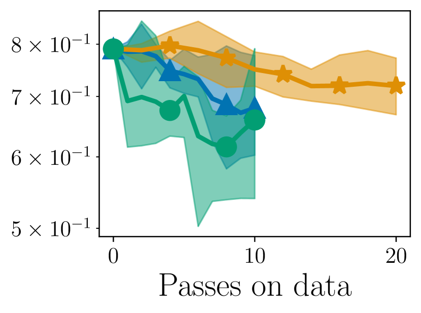
(a) log1
Logistic + L2 ($\lambda=1\text{e-}3$)

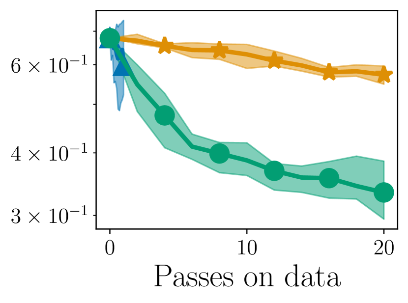
(b) log2
Logistic + L2 ($\lambda=1\text{e-}3$)

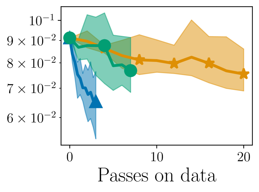
(c) mtp
LS + L2 ($\lambda=5\text{e-}8$)

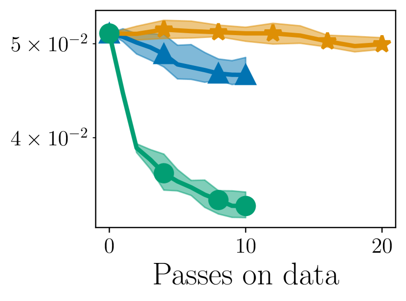
(d) madelon
Logistic + L2 ($\lambda=1$)

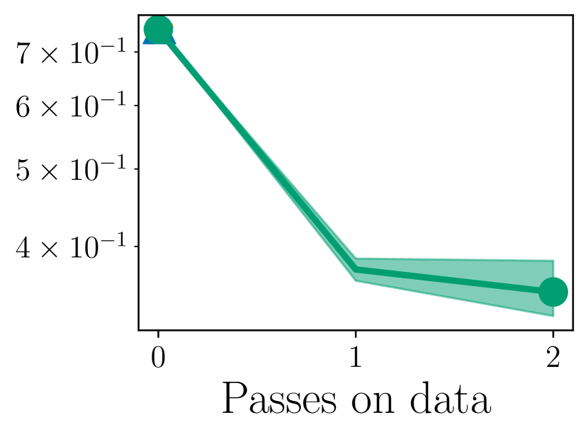
(e) square
LASSO ($\lambda=30$)

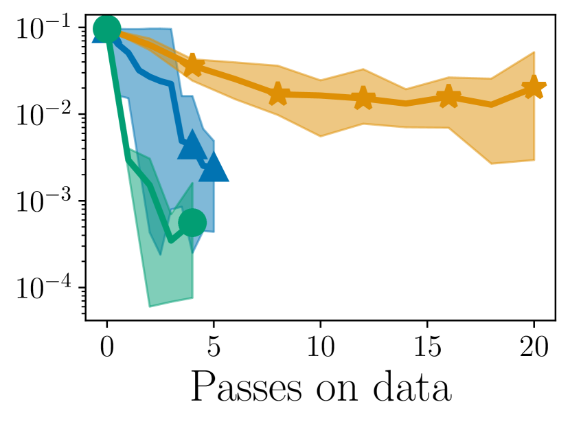
(f) california
LASSO ($\lambda=0.1$)

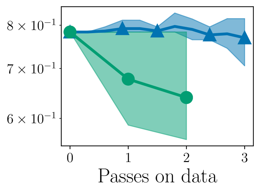
(g) dorothea
Logistic + L1 ($\lambda=0.01$)

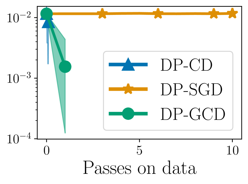
(h) madelon
Logistic + L1 ($\lambda=0.05$)

Figure 1: Relative error (min/mean/max over 5 runs) to non-private optimal for DP-GCD (our approach) versus DP-CD and DP-SGD. On the x-axis, $1$ tick represents a full access to the data: $p$ iterations of DP-CD, $n$ iterations of DP-SGD and $1$ iteration of DP-GCD. Number of iterations, clipping thresholds and step sizes are tuned simultaneously for each algorithm.

DP-GCD exploits problem structure

In the higher-dimensional datasets square and dorothea, where $p\geq n$, DP-GCD is the only algorithm that manages to do multiple iterations and to decrease the objective value (see Figures 1(e) and 1(g)). In both problems, solutions are sparse due to the $\ell_{1}$ regularization. This shows that DP-GCD’s greedy selection of updates can exploit this property to find relevant non-zero coefficients (see Table 3 in Appendix D), even when this selection is noisy. The lower-dimensional datasets log1, log2 and madelon (where $p<n$) are still too high dimensional (relatively to $n$) for DP-SGD and DP-CD to make significant progress. In contrast, DP-GCD exploits the fact that solutions are quasi-sparse to find good approximate solutions quickly (see Figures 1(a), 1(b), 1(d), 1(e), 1(g) and 1(h)). On the low-dimensional dataset california, DP-GCD is roughly on par with DP-SGD and DP-CD (see Figure 1(f)). This is due to the additional noise term introduced by the greedy selection rule: in such setting, the lower number of iterations does not compensate for this as much as in higher-dimensional problems. A similar phenomenon arise in mtp (Figure 1(c)), whose solution is not imbalanced enough for DP-GCD to be superior to its competitors.

Computational complexity

As discussed in Section 4.6, one iteration of DP-GCD requires a full pass on the data. This is as costly as $p$ iterations of DP-CD or $n$ iterations of DP-SGD. Nonetheless, on many problems, DP-GCD requires just as many passes on the data as DP-CD and DP-SGD (Figures 1(a), 1(c), 1(d), 1(e) and 1(f)). When more computation is required, it also provides significantly better solutions than DP-CD and DP-SGD (Figure 1(b)). This is in line with our theoretical results from Section 4.4.

6 Conclusion and Discussion

We proposed DP-GCD, a greedy coordinate descent algorithm for DP-ERM. In favorable settings, DP-GCD achieves utility guarantees of $O(\log(p)/n^{2/3}\epsilon^{2/3})$ and $O(\log(p)/n^{2}\epsilon^{2})$ for convex and strongly-convex objectives. It is the first algorithm to achieve such rates without solving an $\ell_{1}$-constrained problem. Instead, we show that DP-GCD depends on $\ell_{1}$-norm quantities and automatically adapts to the structure of the problem. Specifically, DP-GCD interpolates between logarithmic and polynomial dependence on the dimension, depending on the problem. Thus, DP-GCD constitutes a step towards the design of an algorithm that adjusts to the appropriate $\ell_{p}$ structure of a problem [5, 2, see].

We also showed that DP-GCD adapts to the quasi-sparsity of the problem, without requiring a priori knowledge about it. In such problems, it converges to a good approximate solution in few iterations. This improves utility, and reduces the polynomial dependence on the dimension to a polynomial dependence on the (much smaller) quasi-sparsity level of the solution.

We also proposed and evaluated a proximal variant of DP-GCD, allowing non-smooth, sparsity-inducing regularization. While it is not covered by our utility guarantees, we note that the only existing analysis of such variants in the non-private setting is the one of [27] for $\ell_{1}$ and box constraints. Their proof relies on an alternation between good (that provably progress) and bad steps (that do not increase the objective), which does not transfer to the private setting. Extending such results to DP-ERM is an exciting direction for future work.

Appendix A Proof of Privacy

Theorem 4.2.

Let $\epsilon,\delta\in(0,1]$. Algorithm 1 with $\lambda_{j}=\lambda_{j}^{\prime}=\frac{8L_{j}}{n\epsilon}\sqrt{T\log(1/\delta)}$ is $(\epsilon,\delta)$-DP.

Proof.

In each iteration of Algorithm 1, the data is accessed twice: once to choose the coordinate and once to compute the private gradient. In total, data is thus queried $2T$ times.

Let $\lambda_{j}=\lambda_{j}^{\prime}=\frac{2L_{j}}{n\epsilon^{\prime}}$. For $j\in[p]$, the gradient’s $j$-th entry has sensitivity $2L_{j}$. Thus, by the report noisy max mechanism [15], the greedy choice of $j$ is $\epsilon^{\prime}$-DP. By the Laplace mechanism [15], computing the corresponding gradient coordinate is also $\epsilon^{\prime}$-DP.

The advanced composition theorem for differential privacy thus ensures that the $2T$-fold composition of these mechanisms is $(\epsilon,\delta)$-DP for $\delta>0$ and

$$\epsilon=\sqrt{4T\log(1/\delta)}\epsilon^{\prime}+2T\epsilon^{\prime}(\exp(\epsilon^{\prime})-1)\enspace,$$ (2)

where we recall that $\epsilon^{\prime}=\frac{2L_{j}}{n\lambda_{j}}=\frac{2L_{j}}{n\lambda_{j}^{\prime}}$ for all $j\in[p]$. When $\epsilon\leq 1$, we can give a simpler expression [15, see Corollary 3.21 of]: with $\epsilon^{\prime}={\epsilon}/{4\sqrt{T\log(1/\delta)}}$, Algorithm 1 is $(\epsilon,\delta)$-DP for $\lambda_{j}=\lambda_{j}^{\prime}=8L_{j}\sqrt{T\log(1/\delta)}/{n\epsilon}$. ∎

Appendix B Proof of Utility

In this section, we prove Theorem 4.4 and Theorem 4.7, giving utility upper bounds for DP-GCD. We obtain these high-probability results through a careful examination of the properties of DP-GCD’s iterates, and obtain high-probability results by using concentration inequalities (see Section B.1).

In Section B.2, we prove a general descent lemma, which implies that iterates of DP-GCD converge (with high probability) to a neighborhood of the optimum. This property is proven rigorously in Section B.3.2, and we give the utility results for general convex functions in Section B.3.3. Under the additional assumption that the objective is strongly convex, we prove better utility bounds in Section B.4. These bounds follow from a key lemma (see Section B.4.1), which implies linear convergence to a neighborhood of the optimum. We then use this result in two settings, obtaining two different rates: first in a general setting (in Section B.4.2), then under the additional assumption that the problem’s solution is quasi-sparse (in Section B.4.3).

B.1 Concentration Lemma

To prove high-probability utility results, we first bound (in Lemma B.1) the probability for a sum of squared Laplacian variables to exceed a given threshold.

Lemma B.1.

Let $K>0$ and $\lambda_{1},\dots,\lambda_{K}>0$. Define $X_{k}\sim\operatorname{Lap}(\lambda_{k})$ and $\lambda_{\max}=\max_{k\in[K]}\lambda_{k}$. For any $\beta>0$, it holds that

$$\textnormal{Pr}\left[\sum_{k=1}^{K}X_{k}^{2}\geq\beta\right]\leq 2^{K}\exp\left(-\frac{\sqrt{\beta}}{2\lambda_{\max}}\right)\enspace.$$ (3)

Proof.

We first remark that $(\sum_{k=1}^{K}|X_{k}|)^{2}=\sum_{k=1}^{K}\sum_{k^{\prime}=1}^{K}|X_{k}||X_{k^{\prime}}|\geq\sum_{k=1}^{K}X_{k}^{2}$. Therefore

$$\textnormal{Pr}\left[\sum_{k=1}^{K}X_{k}^{2}\geq a^{2}\right] \leq\textnormal{Pr}\left[\Big{(}\sum_{k=1}^{K}|X_{k}|\Big{)}^{2}\geq a^{2}\right]=\textnormal{Pr}\left[\Big{(}\sum_{k=1}^{K}|X_{k}|\Big{)}\geq a\right]\enspace.$$ (4)

Chernoff’s inequality now gives, for any $\gamma>0$,

$$\textnormal{Pr}\left[\sum_{k=1}^{K}|X_{k}|\geq a\right] \leq\exp(-\gamma a)\mathbb{E}\left[\exp(\gamma\sum_{k=1}^{K}|X_{k}|)\right]\enspace.$$ (5)

By the properties of the exponential and the $X_{k}$’s independence, we can rewrite the inequality as

$$\textnormal{Pr}\left[\sum_{k=1}^{K}|X_{k}|\geq a\right]\leq\exp(-\gamma a)\mathbb{E}\left[\prod_{k=1}^{K}\exp\Big{(}\gamma|X_{k}|\Big{)}\right]=\exp(-\gamma a)\prod_{k=1}^{K}\mathbb{E}\left[\exp\Big{(}\gamma|X_{k}|\Big{)}\right]\enspace.$$ (6)

We can now compute the expectation of $\exp(\gamma|X_{k}|)$ for $k\in[K]$,

$$\mathbb{E}\left[\exp\Big{(}\gamma|X_{k}|\Big{)}\right] =\frac{1}{2\lambda_{k}}\int_{-\infty}^{+\infty}\!\exp(\gamma|x|)\exp(-\frac{|x|}{\lambda_{k}})dx=\frac{1}{\lambda_{k}}\int_{0}^{+\infty}\!\exp\Big{(}(\gamma-\frac{1}{\lambda_{k}})x\Big{)}dx\enspace.$$ (7)

We choose $\gamma=1/2\lambda_{\max}$, such that $\gamma\leq 1/2\lambda_{k}$ for all $k\in[K]$ and obtain

$$\mathbb{E}\left[\exp\Big{(}\gamma|X_{k}|\Big{)}\right] =\frac{1}{\lambda_{k}}\frac{1}{\frac{1}{\lambda_{k}}-\gamma}=\frac{1}{1-\gamma\lambda_{k}}\leq 2\enspace.$$ (8)

Plugging everything together, we have proved that

$$\textnormal{Pr}\left[\sum_{k=1}^{K}X_{k}^{2}\geq a^{2}\right]\leq\textnormal{Pr}\left[\sum_{k=1}^{K}|X_{k}|\geq a\right]\leq 2^{K}\exp(-\frac{a}{2\lambda_{\max}})\enspace,$$ (9)

and taking $a=\sqrt{\beta}$ gives the result. ∎

B.2 Descent Lemma

We now prove a noisy descent lemma for DP-GCD (Lemma B.2). This lemma bounds the suboptimality $f(w^{t+1})-f(w^{*})$ at time $t+1$ as a function of the suboptimality $f(w^{t})-f(w^{*})$ at time $t$, of the gradient’s largest entry and of the noise. At this point, we remark that when the gradient is large enough, it is very probable that $\frac{1}{8}\lVert\nabla f(w^{t})\rVert_{M^{-1},\infty}^{2}\geq\frac{1}{2M_{j}}|\eta_{j}^{t}|^{2}+\frac{1}{2M_{j}}|\chi_{j}^{t}|^{2}+\frac{1}{4M_{j^{*}}}|\chi_{j^{*}}^{t}|^{2}$: this implies that the value of the objective function decreases with high probability, even under the presence of noise. This observation will be crucial for proving utility for general convex functions.

Lemma B.2.

Let $t\geq 0$ and $w^{t},w^{t+1}\in\mathbb{R}^{p}$ two consecutive iterates of Algorithm 1, with $\gamma_{j}=1/M_{j}$ and $\lambda_{j},\lambda_{j}^{\prime}$ chosen as in Theorem 4.2 to ensure $\epsilon,\delta$-DP. We denote by $j\in[p]$ the coordinate chosen at this step $t$, and by $j^{*}=\operatorname*{arg\,max}_{j\in[p]}|\nabla_{j}f(w^{t})|/\sqrt{M_{j}}$ the coordinate that would have been chosen without noise. The following inequality holds

$$f(w^{t+1})-f(w^{*}) \leq f(w^{t})-f(w^{*})-\frac{1}{8}\lVert\nabla f(w^{t})\rVert_{M^{-1},\infty}^{2}+\frac{1}{2M_{j}}|\eta_{j}^{t}|^{2}+\frac{1}{2M_{j}}|\chi_{j}^{t}|^{2}+\frac{1}{4M_{j^{*}}}|\chi_{j^{*}}^{t}|^{2}\enspace.$$ (10)

Proof.

The smoothness of $f$ gives a first inequality

$$f(w^{t+1}) \leq f(w^{t})+\langle\nabla f(w^{t}),w^{t+1}-w^{t}\rangle+\frac{1}{2}\lVert w^{t+1}-w^{t}\rVert_{M}^{2}$$ (11)

$$=f(w^{t})-\frac{1}{M_{j}}\nabla_{j}f(w^{t})(\nabla_{j}f(w^{t})+\eta_{j}^{t})+\frac{1}{2M_{j}}(\nabla_{j}f(w^{t})+\eta_{j}^{t})^{2}$$ (12)

$$=f(w^{t})-\frac{1}{M_{j}}\nabla_{j}f(w^{t})^{2}-\frac{1}{M_{j}}\nabla_{j}f(w^{t})\eta_{j}^{t}+\frac{1}{2M_{j}}(\nabla_{j}f(w^{t}))^{2}$$

$$\quad+\frac{1}{M_{j}}\nabla_{j}f(w^{t})\eta_{j}^{t}+\frac{1}{2M_{j}}(\eta_{j}^{t})^{2}$$ (13)

$$=f(w^{t})-\frac{1}{2M_{j}}\nabla_{j}f(w^{t})^{2}+\frac{1}{2M_{j}}(\eta_{j}^{t})^{2}\enspace.$$ (14)

We will make the noisy gradient appear, so as to use the noisy greedy rule. To do so, we remark that the classical inequality $(a+b)^{2}\leq 2a^{2}+2b^{2}$ for any $a,b\in\mathbb{R}$ implies that $-a^{2}\leq-\frac{1}{2}(a+b)^{2}+b^{2}$. Applied with $a=\nabla_{j}f(w^{t})/\sqrt{M_{j}}$ and $b=\chi_{j}^{t}/\sqrt{M_{j}}$, this results in

$$-\frac{1}{2M_{j}}\nabla_{j}f(w^{t})^{2} \leq-\frac{1}{4M_{j}}(\nabla_{j}f(w^{t})+\chi_{j}^{t})^{2}+\frac{1}{2M_{j}}(\chi_{j}^{t})^{2}\enspace.$$ (15)

And, by the noisy greedy rule, $\frac{1}{\sqrt{M_{j^{*}}}}|\nabla_{j^{*}}f(w^{t})+\chi_{j^{*}}^{t}|\leq\frac{1}{\sqrt{M_{j}}}|\nabla_{j}f(w^{t})+\chi_{j}^{t}|$. We replace in (15) and use the inequality $-a^{2}\leq-\frac{1}{2}(a+b)^{2}+b^{2}$ with $a=(\nabla_{j^{*}}f(w^{t})+\chi_{j^{*}})/\sqrt{M_{j^{*}}}$ and $b=-\chi_{j^{*}}/\sqrt{M_{j^{*}}}$ to obtain

$$-\frac{1}{2M_{j}}\nabla_{j}f(w^{t})^{2} \leq-\frac{1}{4M_{j^{*}}}(\nabla_{j^{*}}f(w^{t})+\chi_{j^{*}}^{t})^{2}+\frac{1}{2M_{j}}(\chi_{j}^{t})^{2}$$ (16)

$$\leq-\frac{1}{8M_{j^{*}}}(\nabla_{j^{*}}f(w^{t}))^{2}+\frac{1}{4M_{j^{*}}}(\chi_{j^{*}}^{t})^{2}+\frac{1}{2M_{j}}(\chi_{j}^{t})^{2}\enspace.$$ (17)

The result follows from (14) and $\frac{1}{M_{j^{*}}}(\nabla_{j^{*}}f(w^{t}))^{2}=\lVert\nabla f(w^{t})\rVert_{M^{-1},\infty}^{2}$. ∎

B.3 Utility for General Convex Functions

In this section, we derive an upper bound on the utility of DP-GCD for convex objective functions. First, we use convexity of $f$ to upper bound the decrease described in Lemma B.2. This gives Lemma B.3 in Section B.3.1, where the suboptimality gap $f(w^{t+1})-f(w^{*})$ at time $t+1$ is upper bound by a function of the suboptimality gap $f(w^{t})-f(w^{*})$ at time $t$ and the noise injected in step $t$. The novelty of our analysis lies in Lemma B.4, where examine the decrease of the objective. Specifically, we show that either (i) $f(w^{t})$ is far from its minimum, and the suboptimality gap decreases with high probability, either (ii) $f(w^{t})$ is close to its minimum, then all future iterates of DP-GCD will remain in a ball whose radius is determined by the variance of the noise. This observation is essential for proving the utility results stated in Section 4.3.

B.3.1 Descent Lemma for Convex Functions

Lemma B.3.

Under the hypotheses of Lemma B.2, for a convex objective function $f$, we have

$$f(w^{t+1})-f(w^{*}) \leq f(w^{t})-f(w^{*})-\frac{(f(w^{t})-f(w^{*}))^{2}}{8\lVert w^{t}-w^{*}\rVert_{M,1}^{2}}$$

$$\quad+\frac{1}{2M_{j}}|\eta_{j}^{t}|^{2}+\frac{1}{2M_{j}}|\chi_{j}^{t}|^{2}+\frac{1}{4M_{j^{*}}}|\chi_{j^{*}}^{t}|^{2}\enspace.$$ (18)

Proof.

Since $f$ is convex, it holds that

$$f(w^{*}) \geq f(w^{t})+\langle\nabla f(w^{t}),w^{*}-w^{t}\rangle\enspace.$$ (19)

After reorganizing the terms, we can upper bound them using Hölder’s inequality

$$f(w^{t})-f(w^{*}) \leq\langle\nabla f(w^{t}),w^{t}-w^{*}\rangle$$ (20)

$$\leq\lVert\nabla f(w^{t})\rVert_{M^{-1},\infty}\lVert w^{t}-w^{*}\rVert_{M,1}\enspace,$$ (21)

where the second inequality holds since $\lVert\cdot\rVert_{M,1}$ and $\lVert\cdot\rVert_{M^{-1},\infty}$ are conjugate norms. We now divide (21) by $\lVert w^{t}-w^{*}\rVert_{M,1}$, square it and reorganize to get $-\lVert\nabla f(w^{t})\rVert_{M^{-1},\infty}^{2}\leq-\frac{(f(w^{t})-f(w^{*}))^{2}}{\lVert w^{t}-w^{*}\rVert_{M,1}^{2}}$. Replacing in Lemma B.2 gives the result. ∎

B.3.2 Key Lemma on the Behavior of DP-GCD’s Iterates

Now that we have an inequality in the form of Lemma B.3, we prove that iterates of DP-GCD converge to a vicinity of the optimum. In the general lemma below, think of $\xi_{t}$ as $f(w^{t})-f(w^{*})$ and of $\beta$ as the variance of the term. This result will be combined with Lemma B.1 to obtain high-probability bounds.

Lemma B.4.

Let $\{c_{t}\}_{t\geq 0}$ and $\{\xi_{t}\}_{t\geq 0}$ be two sequences of positive values that satisfy, for all $t\geq 0$,

$$\xi_{t+1}\leq\xi_{t}-\frac{\xi_{t}^{2}}{c_{t}}+\beta,$$ (22)

such that if $\xi_{t}\leq\xi_{0}$ then $c_{t}\leq c_{0}$. Assume that $\beta\leq c_{0}$ and $\xi_{0}\geq 2\sqrt{\beta c_{0}}$. Then:

1. For all $t>0$, $c_{t}\leq c_{0}$, and there exists $t^{*}>0$ such that $\xi_{t+1}\leq\xi_{t}$ if $t<t^{*}$ and $\xi_{t}\leq 2\sqrt{\beta c_{0}}$ if $t\geq t^{*}$.

2. For all $t\geq 1$, $\xi_{t}\leq\frac{c_{0}}{t}+2\sqrt{\beta c_{0}}$.

Proof.

1. Assume that for $t\geq 0$, $\sqrt{\beta c_{0}}\leq\xi_{t}\leq\xi_{0}$. Then,

$$\xi_{t+1}\leq\xi_{t}-\frac{\xi_{t}^{2}}{c_{t}}+\beta\leq\xi_{t}-\frac{\sqrt{\beta c_{0}}^{2}}{c_{0}}+\beta=\xi_{t}\enspace,$$ (23)

where the second inequality comes from $\xi_{t}\geq\sqrt{\beta c_{0}}$ and $\xi_{t}\leq\xi_{0}$ (which implies $c_{t}\leq c_{0}$). We now define the following value $t^{*}$, which defines the point of rupture between two regimes for $\xi_{t}$:

$$t^{*}=\min\left\{t\geq 0\,\middle|\,\xi_{t}\leq\sqrt{\beta c_{0}}\right\}\enspace.$$ (24)

Let $t<t^{*}$, assume that $\xi_{t}\leq\xi_{0}$, then (23) holds, that is $\xi_{t+1}\leq\xi_{t}\leq\xi_{0}$. By induction, it follows that for all $t<t^{*}$, $\xi_{t+1}\leq\xi_{t}\leq\xi_{0}$ and $c_{t}\leq c_{0}$.

Remark now that $\xi_{t^{*}}\leq\sqrt{\beta c_{0}}$, we prove by induction that $\xi_{t}$ stays under $2\sqrt{\beta c_{0}}$ for $t\geq t^{*}$. Assume that for $t\geq t^{*}$, $\xi_{t}\leq 2\sqrt{\beta c_{0}}$. Then, there are two possibilities. If $\xi_{t}\leq\sqrt{\beta c_{0}}$, then

$$\xi_{t+1}\leq\xi_{t}-\frac{\xi_{t}^{2}}{c_{t}}+\beta\leq\sqrt{\beta c_{0}}+\beta\leq 2\sqrt{\beta c_{0}}\enspace,$$ (25)

and $\xi_{t+1}\leq 2\sqrt{\beta c_{0}}$. Otherwise, $\sqrt{\beta c_{0}}\leq\xi_{t}\leq 2\sqrt{\beta c_{0}}\leq\xi_{0}$ and (23) holds, which gives $\xi_{t+1}\leq\xi_{t}\leq 2\sqrt{\beta c_{0}}$. We proved that for $t\geq t^{*}$, $\xi_{t}\leq 2\sqrt{\beta c_{0}}$, which concludes the proof of the first part of the lemma.

2. We start by proving this statement for $0<t<t^{*}-1$. Define $\omega=\frac{2u}{c_{0}}$ and $u=\sqrt{\beta c_{0}}$. The assumption on $\xi_{t}$ implies, by the first part of the lemma, $\xi_{t+1}\leq\xi_{t}-\frac{\xi_{t}^{2}}{c_{t}}+\beta\leq\xi_{t}-\frac{\xi_{t}^{2}}{c_{0}}+\beta$, which can be rewritten

$$\xi_{t+1}-u\leq(1-\omega)(\xi_{t}-u)-\frac{(\xi_{t}-u)^{2}}{c_{0}}\enspace,$$ (26)

since $(1-\omega)(\xi_{t}-u)-\frac{(\xi_{t}-u)^{2}}{c_{0}}=\xi_{t}-\omega\xi_{t}-u+\omega u-\frac{\xi_{t}^{2}}{c_{0}}-\frac{2\xi_{t}u}{c_{0}}-\frac{u^{2}}{c_{0}}=\xi_{t}-\frac{\xi_{t}^{2}}{c_{0}}-u+\omega u-\frac{u^{2}}{c_{0}}$, and $\omega u-\frac{u^{2}}{c_{0}}=\frac{u^{2}}{c_{0}}=\beta$. Since $t<t^{*}-1$, $\xi_{t+1}-u>0$ and $\xi_{t}-u>0$, we can thus divide  (26) by $(\xi_{t+1}-u)(\xi_{t}-u)$ to obtain

$$\frac{1}{\xi_{t}-u}\leq\frac{1-\omega}{\xi_{t+1}-u}-\frac{\xi_{t}-u}{(\xi_{t+1}-u)c_{0}}\leq\frac{1-\omega}{\xi_{t+1}-u}-\frac{1}{c_{0}}\leq\frac{1}{\xi_{t+1}-u}-\frac{1}{c_{0}}\enspace,$$ (27)

where the second inequality comes from $\xi_{t+1}-u\leq\xi_{t}-u$ from the first part of the lemma. By applying this inequality recursively and taking the inverse of the result, we obtain the desired resuld $\xi_{t}\leq\frac{c_{0}}{t}+\sqrt{\beta c_{0}}\leq\frac{c_{0}}{t}+2\sqrt{\beta c_{0}}$ for all $0<t<t^{*}$.

For $t\geq t^{*}$, we have already proved that $\xi_{t}\leq 2\sqrt{\beta c_{0}}\leq\frac{c_{0}}{t}+2\sqrt{\beta c_{0}}$, which concludes our proof. ∎

B.3.3 Convex Utility Result

Theorem 4.4.

(Convex Case) Let $\epsilon,\delta\in(0,1]$. Assume $\ell(\cdot;d)$ is a convex and $L$-component-Lipschitz loss function for all $d\in\mathcal{X}$, and $f$ is $M$-component-smooth. Define $\mathcal{W}^{*}$ the set of minimizers of $f$, and $f^{*}$ the minimum of $f$. Let $w_{priv}\in\mathbb{R}^{p}$ be the output of Algorithm 1 with step sizes $\gamma_{j}={1}/{M_{j}}$, and noise scales $\lambda_{1},\dots,\lambda_{p},\lambda_{1}^{\prime},\dots,\lambda_{p}^{\prime}$ set as in Theorem 4.2 (with $T$ chosen below) to ensure $(\epsilon,\delta)$-DP. Then, the following holds for $\zeta\in(0,1]$:

$$f(w_{priv})-f(w^{*})\leq\frac{8R_{M}^{2}}{T}+\sqrt{32R_{M}^{2}\beta}\enspace,$$ (28)

where $\beta=\frac{2\lambda_{\max}^{2}}{M_{\min}}\log(\frac{8Tp}{\zeta})^{2}$, and $\displaystyle R_{M}=\max_{w\in\mathbb{R}^{p}}\min_{w^{*}\in\mathcal{W}^{*}}\left\{\lVert w-w^{*}\rVert_{M,1}\mid f(w)\leq f(w^{0})\right\}$. If we set $T=\Big{(}\frac{n^{2}\epsilon^{2}R_{M}^{2}M_{\min}}{2^{7}L_{\max}^{2}\log(1/\delta)}\Big{)}^{{1}/{3}}$, then with probability at least $1-\zeta$,

$$f(w^{T})-f(w^{0})=\widetilde{O}\Big{(}\frac{R_{M}^{4/3}L_{\max}^{2/3}\log(p/\zeta)}{M_{\min}^{1/3}n^{2/3}\epsilon^{2/3}}\Big{)}\enspace.$$ (29)

Proof.

Let $\xi_{t}=f(w^{t})-f(w^{*})$. We upper bound the following probability by the union bound, and the fact that for $t\geq 0$, the events $E_{j}^{t}:$ “coordinate $j$ is updated at step $t$” for $j\in[p]$ partition the probability space:

$$\textnormal{Pr}\left[\exists t,\xi_{t+1}\geq\xi_{t}-\frac{\xi_{t}^{2}}{8\lVert w^{t}-w^{*}\rVert_{M,1}^{2}}+\beta\right]\leq\sum_{t=0}^{T-1}\textnormal{Pr}\left[\xi_{t+1}\geq\xi_{t}-\frac{\xi_{t}^{2}}{8\lVert w^{t}-w^{*}\rVert_{M,1}^{2}}+\beta\right]$$ (30)

$$=\sum_{t=0}^{T-1}\sum_{j=1}^{p}\textnormal{Pr}\left[\xi_{t+1}\geq\xi_{t}-\frac{\xi_{t}^{2}}{8\lVert w^{t}-w^{*}\rVert_{M,1}^{2}}+\beta~{}\land~{}E_{j}^{t}\right]\enspace.$$ (31)

Lemma B.3 gives $\xi_{t+1}\leq\xi_{t}-\frac{\xi_{t}^{2}}{8\lVert w^{t}-w^{*}\rVert_{M,1}^{2}}+\frac{1}{2M_{j}}|\eta_{j}^{t}|^{2}+\frac{1}{2M_{j}}|\chi_{j}^{t}|^{2}+\frac{1}{4M_{j^{*}}}|\chi_{j^{*}}^{t}|^{2}$. We thus have the following upper bound:

$$\textnormal{Pr}\left[\exists t,\xi_{t+1}\geq\xi_{t}-\tfrac{1}{8\lVert w^{t}-w^{*}\rVert_{M,1}^{2}}\xi_{t}^{2}+\beta\right]\leq\sum_{t=0}^{T-1}\sum_{j=1}^{p}\textnormal{Pr}\left[\tfrac{|\eta_{j}^{t}|^{2}}{2M_{j}}+\tfrac{|\chi_{j}^{t}|^{2}}{2M_{j}}+\tfrac{|\chi_{j^{*}}^{t}|^{2}}{4M_{j^{*}}}\geq\beta\right]$$ (32)

$$\leq\sum_{t=0}^{T-1}\sum_{j=1}^{p}\textnormal{Pr}\left[|\eta_{j}^{t}|^{2}+|\chi_{j}^{t}|^{2}+|\chi_{j^{*}}^{t}|^{2}\geq 2M_{\min}\beta\right]\enspace.$$ (33)

By Lemma B.1 with $X_{1}=\eta_{j}^{t}\sim\operatorname{Lap}(\lambda_{j})$, $X_{2}=\chi_{j}^{t}\sim\operatorname{Lap}(\lambda_{j}^{\prime})$ and $X_{3}=\chi_{j^{*}}^{t}\sim\operatorname{Lap}(\lambda_{j^{*}}^{\prime})$, it holds that

$$\textnormal{Pr}\left[|\eta_{j}^{t}|^{2}+|\chi_{j}^{t}|^{2}+|\chi_{j^{*}}^{t}|^{2}\geq 2M_{\min}\beta\right] \leq 8\exp\left(-\frac{\sqrt{2M_{\min}\beta}}{2\lambda_{\max}}\right)=\frac{\zeta}{Tp}\enspace,$$ (34)

where the last equality comes from $\beta=\frac{2\lambda_{\max}^{2}}{M_{\min}}\log(\frac{8Tp}{\zeta})^{2}$. We have proved that

$$\textnormal{Pr}\left[\exists t,\xi_{t+1}\geq\xi_{t}-\frac{\xi_{t}^{2}}{8\lVert w^{t}-w^{*}\rVert_{M,1}^{2}}+\beta\right] \leq\sum_{t=0}^{T-1}\sum_{j=1}^{p}\frac{\zeta}{Tp}=\zeta\enspace.$$ (35)

We now use our Lemma B.4, with $\xi_{t}=f(w^{t})-f(w^{*})$; $c_{0}=8R_{M}^{2}$ and $c_{t}=8\lVert w^{t}-w^{*}\rVert_{M,1}^{2}$ for $t>0$; and $\beta=\frac{2\lambda_{\max}^{2}}{M_{\min}}\log(\frac{8Tp}{\zeta})^{2}$. These values satisfies the assumptions of Lemma B.4 since, by the definition of $R_{M}$, it holds that $c_{t}\leq c_{0}$ whenever $\xi_{t}\leq\xi_{0}$ (i.e., $f(w^{t})-f(w^{*})\leq f(w^{0})-f(w^{*})$). Additionally, $f(w^{0})-f(w^{*})\geq\sqrt{32R_{M}^{2}\beta}$, therefore $f(w^{0})-f(w^{*})\geq 2\sqrt{\beta c_{0}}$, and $\beta\leq c_{0}$.

We obtain the result, with probability at least $1-\zeta$:

$$f(w^{t})-f(w^{0}) \leq\frac{c_{0}}{t}+2\sqrt{\beta c_{0}}=\frac{8R_{M}^{2}}{t}+\frac{64R_{M}L_{\max}\log(8Tp/\zeta)\sqrt{T\log(1/\delta)}}{\sqrt{M_{\min}}n\epsilon}\enspace.$$ (36)

For $T=\frac{R_{M}^{2/3}M_{\min}^{1/3}n^{2/3}\epsilon^{2/3}}{4L_{\max}^{2/3}\log(1/\delta)^{1/3}}$, we obtain that, with probability at least $1-\zeta$,

$$f(w^{t})-f(w^{0}) \leq\frac{64R_{M}^{4/3}L_{\max}^{2/3}\log(1/\delta)^{1/3}}{M_{\min}^{1/3}n^{2/3}\epsilon^{2/3}}\log\Big{(}\frac{pR_{M}^{2/3}M_{\min}^{1/3}n^{2/3}\epsilon^{2/3}}{4\zeta L_{\max}^{2/3}\log(1/\delta)^{1/3}}\Big{)}\enspace,$$ (37)

which is the result of the theorem. ∎

B.4 Utility for Strongly-Convex Functions

B.4.1 A Key Inequality for Strongly-Convex Functions

We now prove a link between $f$’s largest gradient entry and the suboptimality gap, under the assumption that there exists a unique minimizer $w^{*}$ of $f$ that is $(\alpha,\tau)$-quasi-sparse. Note that this assumption is not restrictive in general as any vector in $\mathbb{R}^{p}$ is $(0,p)$-quasi-sparse, and for any $\tau$ there exists $\alpha>0$ such that the vector is $(\alpha,\tau)$-quasi-sparse. We will denote by $\mathcal{W}_{\tau,\alpha}\subseteq\mathbb{R}^{p}$ the set of $(\alpha,\tau)$-quasi-sparse vectors of $\mathbb{R}^{p}$:

$$\mathcal{W}_{\tau,\alpha}=\left\{w\in\mathbb{R}^{p}\mid|\{j\in[p]\mid|w_{j}|\geq\alpha\}|\leq\tau\right\}\enspace.$$ (38)

When $\alpha=0$, we simply write $\mathcal{W}_{\tau}=\mathcal{W}_{\tau,0}$, that is the set of $\tau$-sparse vectors. We also define the associated thresholding operator $\pi_{\alpha}$, that puts to $0$ the coordinates that are smaller than $\alpha$, “projecting” vectors from $\mathcal{W}_{\tau,\alpha}$ to $\mathcal{W}_{\tau}$, i.e., for $w\in\mathbb{R}^{p}$,

$$\pi_{\alpha}(w)=\begin{cases}0&\text{if }|w_{j}|\leq\alpha\enspace,\\ w_{j}&\text{otherwise}\enspace.\end{cases}$$ (39)

Importantly, restricting a function to $\tau$-sparse vectors changes its strong-convexity parameter. Let $\tau\geq 0$ and $q\in\{1,2\}$, we say a function is $\mu_{M,q}^{(\tau)}$-strongly-convex when restricted to $\tau$-sparse vectors if for all $\tau$-sparse vectors $v,w\in\mathcal{W}_{\tau}$,

$$f(w) \geq f(v)+\langle\nabla f(v),w-v\rangle+\frac{\mu_{M,q}^{(\tau)}}{2}\lVert w-v\rVert_{M,q}^{2}\enspace.$$ (40)

Remark that when $\tau\geq p$, we recover the usual strong-convexity parameters. The parameters w.r.t. $\ell_{1}$- and $\ell_{2}$-norms can be compared using the following inequality [16], for all $\tau\geq 0$,

$$\frac{1}{\tau}\mu_{M,2}^{(\tau)} \leq\mu_{M,1}^{(\tau)}\leq\mu_{M,2}^{(\tau)}\enspace.$$ (41)

We are ready to prove Lemma B.5.

Lemma B.5.

Let $f:\mathbb{R}^{p}\rightarrow\mathbb{R}$ be a function that is $M$-component-smooth, and $\mu_{M,1}^{(\tau)}$-strongly-convex w.r.t. $\lVert\cdot\rVert_{M,1}$ when restricted to $\tau$-sparse vectors, for $\tau\geq 0$. Assume that the unique minimizer $w^{*}$ of $f$ is $(\tau,\alpha)$-quasi-sparse, for $\alpha,\tau\geq 0$. Let $w^{t}\in\mathbb{R}^{p}$ be a $t$-sparse vector for some $t\geq 0$. Then we have

$$-\frac{1}{2}\lVert\nabla f(w^{t})\rVert_{M^{-1},\infty} \leq-\mu_{M,1}^{(t+\tau)}(f(w^{t})-f(w^{*}))+\frac{1}{2}M_{\max}\mu_{M,1}^{(t+\tau)}(p-\tau)\alpha^{2}\enspace.$$ (42)

Proof.

Let $w^{t}\in\mathbb{R}^{p}$ be a $t$-sparse vector. Remark that $w^{*}$ is $(\alpha,\tau)$-quasi-sparse, meaning that $\pi_{\alpha}(w^{*})$ is $\tau$-sparse. The union of $w^{t}$ and $\pi_{\alpha}(w^{*})$’s supports ($\mathop{\rm supp}(w^{t})$ and $\mathop{\rm supp}(\pi_{\alpha}(w^{*}))$) thus satisfies $|\mathop{\rm supp}(w)\cup\mathop{\rm supp}(\pi_{\alpha}(w^{*}))|\leq t+\tau$. As the function $f$ is $\mu_{M,1}^{(t+\tau)}$-strongly-convex with respect to $\lVert\cdot\rVert_{M,1}$ and $t+\tau$ sparse vector,

$$f(\pi_{\alpha}(w))\geq f(w^{t})+\langle\nabla f(w^{t}),\pi_{\alpha}(w)-w^{t}\rangle+\frac{\mu_{M,1}^{(t+\tau)}}{2}\lVert\pi_{\alpha}(w)-w^{t}\rVert_{M,1}^{2}\enspace.$$ (43)

Since $\pi_{\alpha}:\mathcal{W}_{\tau,\alpha}\rightarrow\mathcal{W}_{\tau,0}$ is surjective, minimizing this equation for $w\in\mathcal{W}_{\tau,\alpha}$ on both sides gives

$$\inf_{w\in\mathcal{W}_{\tau}}f(w) \geq f(w^{t})-\sup_{w\in\mathcal{W}_{\tau,\alpha}}\left\{\langle-\nabla f(w^{t}),w^{t}-\pi_{\alpha}(w)\rangle-\frac{\mu_{M,1}^{(t+\tau)}}{2}\lVert\pi_{\alpha}(w)-w^{t}\rVert_{M,1}^{2}\right\}$$ (44)

$$\geq f(w^{t})-\sup_{w\in\mathbb{R}^{p}}\left\{\langle-\nabla f(w^{t}),w^{t}-w\rangle-\frac{\mu_{M,1}^{(t+\tau)}}{2}\lVert w-w^{t}\rVert_{M,1}^{2}\right\}\enspace.$$ (45)

The second term corresponds to the conjugate of the function $\frac{1}{2}\lVert\cdot\rVert_{M,1}^{2}$, that is $\frac{1}{2}\lVert\cdot\rVert_{M^{-1},\infty}^{2}$ [9]. This gives

$$\inf_{w\in\mathcal{W}_{\tau}}f(w) \geq f(w^{t})-\left(\frac{\mu_{M,1}^{(t+\tau)}}{2}\lVert\cdot\rVert_{1}^{2}\right)^{*}(-\nabla f(w^{\prime}))$$ (46)

$$=f(w^{t})-\frac{1}{2\mu_{M,1}^{(t+\tau)}}\lVert\nabla f(w^{\prime})\rVert_{M^{-1},\infty}^{2}\enspace.$$ (47)

Finally, $w^{*}$ is the minimizer of $f$ (which is convex), thus $\nabla f(w^{*})=0$. The smoothness of $f$ gives, for any $w\in\mathbb{R}^{p}$, $f(w)\leq f(w^{*})+\frac{1}{2}\lVert w-w^{*}\rVert_{M,2}^{2}$. Hence

$$\inf_{w\in\mathcal{W}_{\tau}}f(w)\leq f(w^{*})+\inf_{w\in\mathcal{W}_{\tau}}\frac{1}{2}\lVert w-w^{*}\rVert_{M,2}^{2}.\leq f(w^{*})+\frac{1}{2}\lVert\pi_{\alpha}(w^{*})-w^{*}\rVert_{M,2}^{2}\enspace,$$ (48)

where the second inequality comes from $\pi_{\alpha}(w^{*})\in\mathcal{W}_{\tau}$, since $w^{*}\in\mathcal{W}_{\tau,\alpha}$. It remains to observe that $\lVert\pi_{\alpha}(w^{*})-w^{*}\rVert_{M,2}^{2}\leq M_{\max}(p-\tau)\alpha^{2}$ to get the result. ∎

Corollary B.6.

For $\tau$-sparse vectors, we have $\alpha=0$ and thus $(p-\tau)\alpha=0$. Lemma B.5 can thus be simplified as

$$-\frac{1}{2}\lVert\nabla f(w^{t})\rVert_{M^{-1},\infty}^{2} \leq-\mu_{M,1}^{(t+\tau)}(f(w^{t})-f(w^{*}))\enspace.$$ (49)

When vectors are not sparse ($\tau=p$), we recover the inequality $-\frac{1}{2}\lVert\nabla f(w^{t})\rVert_{M^{-1},\infty}^{2}\leq-\mu_{M,1}(f(w^{t})-f(w^{*}))$.

B.4.2 General Strongly-Convex Utility Result

Theorem 4.4.

(Strongly-Convex Case) Let $\epsilon,\delta\in(0,1]$. Assume $\ell(\cdot;d)$ is a $\mu_{M,1}$-strongly-convex w.r.t. $\lVert\cdot\rVert_{M,1}$ and $L$-component-Lipschitz loss function for all $d\in\mathcal{X}$, and $f$ is $M$-component-smooth. Let $\mathcal{W}^{*}$ be the set of minimizers of $f$, and $f^{*}$ the minimum of $f$. Let $w_{priv}\in\mathbb{R}^{p}$ be the output of Algorithm 1 with step sizes $\gamma_{j}={1}/{M_{j}}$, and noise scales $\lambda_{1},\dots,\lambda_{p},\lambda_{1}^{\prime},\dots,\lambda_{p}^{\prime}$ set as in Theorem 4.2 (with $T$ chosen below) to ensure $(\epsilon,\delta)$-DP. Then, the following holds for $\zeta\in(0,1]$:

$$f(w^{T})-f(w^{*})\leq(1-\frac{\mu_{M,1}}{2})^{T}(f(w^{0})-f(w^{*}))+\frac{64TL_{\max}^{2}\log(1/\delta)}{M_{\min}\mu_{M,1}n^{2}\epsilon^{2}}\log(\frac{2Tp}{\zeta})\enspace.$$ (50)

If we set $T=\frac{2}{\mu_{M,1}}\log(\frac{M_{\min}\mu_{M,1}n^{2}\epsilon^{2}(f(w^{0})-f(w^{*})}{32L_{\max}^{2}\log(1/\delta)})$, then with probability at least $1-\zeta$,

$$f(w^{T})-f(w^{*}) =\widetilde{O}\Big{(}\frac{L_{\max}^{2}\log(p/\zeta)}{M_{\min}\mu_{M,1}^{2}n^{2}\epsilon^{2}}\Big{)}\enspace.$$ (51)

Proof.

When $f$ is $\mu_{M,1}$-strongly-convex w.r.t. the norm $\lVert\cdot\rVert_{M,1}$, Corollary B.6 with $\tau=p$ and $\alpha=0$ (which holds for any vector) yields

$$-\frac{1}{2}\lVert\nabla f(w^{t})\rVert_{M^{-1},\infty}^{2} \leq-\mu_{M,1}(f(w^{t})-f(w^{*}))\enspace.$$ (52)

We replace this in Lemma B.2 to obtain

$$f(w^{t+1})-f(w^{*}) \leq(1-\frac{\mu_{M,1}}{4})(f(w^{t})-f(w^{*}))+\frac{1}{2M_{j}}|\eta_{j}^{t}|^{2}+\frac{1}{2M_{j}}|\chi_{j}^{t}|^{2}+\frac{1}{4M_{j^{*}}}|\chi_{j^{*}}^{t}|^{2}\enspace.$$ (53)

Analogously to the proof of 4.4, we define $\xi_{t}=f(w^{t})-f(w^{*})$ for all $0\leq t\leq T$, and show that $\textnormal{Pr}\left[\exists t,\xi_{t+1}\geq(1-\frac{\mu_{M,1}}{4})\xi_{t}+\beta\right]\leq\zeta/Tp$, with $\beta=\frac{2\lambda_{\max}^{2}}{M_{\min}}\log(\frac{8Tp}{\zeta})^{2}$. This yields that, with probability at least $1-\zeta$,

$$f(w^{T})-f(w^{*}) \leq(1-\frac{\mu_{M,1}}{4})^{T}(f(w^{0})-f(w^{*}))+\sum_{t=0}^{T-1}(1-\frac{\mu_{M,1}}{4})^{T-t}\beta$$ (54)

$$\leq(1-\frac{\mu_{M,1}}{4})^{T}(f(w^{0})-f(w^{*}))+\frac{4}{\mu_{M,1}}\frac{32TL_{\max}^{2}\log(1/\delta)}{M_{\min}n^{2}\epsilon^{2}}\log\Big{(}\frac{8Tp}{\zeta}\Big{)}^{2}\enspace,$$ (55)

With $T=\frac{4}{\mu_{M,1}}\log\Big{(}\frac{\mu_{M,1}M_{\min}n^{2}\epsilon^{2}(f(w^{0})-f(w^{*}))}{128L_{\max}^{2}\log(1/\delta)\log(8p/\zeta)}\Big{)}$ we have, with probability at least $1-\zeta$,

$$f(w^{T})-f(w^{*}) \leq\frac{128L_{\max}^{2}\log(1/\delta)\log(8p/\zeta)^{2}}{\mu_{M,1}M_{\min}n^{2}\epsilon^{2}}$$

$$\quad+\frac{512L_{\max}^{2}\log(1/\delta)\log(8Tp/\zeta)^{2}}{\mu_{M,1}^{2}M_{\min}n^{2}\epsilon^{2}}\log\Big{(}\frac{\mu_{M,1}M_{\min}n^{2}\epsilon^{2}(f(w^{0})-f(w^{*}))}{128L_{\max}^{2}\log(1/\delta)\log(8p/\zeta)^{2}}\Big{)}\enspace,$$ (56)

which is the desired result. ∎

B.4.3 Better Utility for Quasi-Sparse Solutions

Theorem 4.7.

Consider $f$ satisfying the hypotheses of Theorem 4.4, with Algorithm 1 initialized at $w^{0}=0$. We denote its output $w^{T}$, and assume that its iterates remain $s$-sparse for some $s\leq p$. Assume that, for all $\tau^{\prime}\geq 0$, $f$ is $\mu_{M,1}^{(\tau^{\prime})}$-strongly-convex w.r.t. $\lVert\cdot\rVert_{M,1}$ for $\tau^{\prime}$-sparse vectors and $\mu_{M,2}$-strongly-convex w.r.t. $\lVert\cdot\rVert_{M,2}$, and that the (unique) solution of problem (1) is $(\alpha,\tau)$-quasi-sparse for some $\alpha,\tau\geq 0$. Let $T\geq 0$, $\zeta\in[0,1]$, and $\beta=\frac{2\lambda_{\max}^{2}}{M_{\min}}\log(TP/\zeta)^{2}$. Then for all $t\leq T$ we have that, with probability at least $1-\zeta$:

$$f(w^{T}) -f(w^{*})\leq\Big{(}1-\frac{\mu_{M,1}^{(\min(s,T)+\tau)}}{4}\Big{)}^{T}(f(w^{0})-f(w^{*}))+\frac{4(\min(s,T)+\tau)\beta}{\mu_{M,2}}+\frac{\min(s,T)+\tau}{8}(p-\tau)\alpha^{2}$$ (57)

$$\leq\Big{(}1-\frac{\mu_{M,2}}{4(\min(s,T)+\tau)}\Big{)}^{T}(f(w^{0})-f(w^{*}))+\frac{4(\min(s,T)+\tau)\beta}{\mu_{M,2}}+\frac{\min(s,T)+\tau}{8}(p-\tau)\alpha^{2}\enspace.$$ (58)

Setting $T=\frac{s+\tau}{\mu_{M,2}}\log((f(w^{0})-f^{*})M_{\min}\mu_{M,2}n^{2}\epsilon^{2}/L^{2})$, and assuming $\alpha^{2}=O\left(L_{\max}^{2}(s+\tau)/M_{\min}\mu_{M,2}^{2}pn^{2}\epsilon^{2}\right)$, we obtain that with probability at least $1-\zeta$,

$$f(w^{T})-f^{*}=\widetilde{O}\left(\frac{L_{\max}^{2}}{M_{\min}}\frac{(s+\tau)^{2}\log(2p/\zeta)}{\mu_{M,2}n^{2}\epsilon^{2}}\right)\enspace.$$ (59)

Proof.

First, we remark that at each iteration, we change only one coordinate. Therefore, after $t$ iterations, the iterate $w^{t}$ is at most $t$-sparse. Since all iterates are also $s$-sparse, it is $\min(s,t)$-sparse. Additionally, we assumed that $w^{*}$ is $(\tau,\alpha)$-almost-sparse. Therefore, Lemma B.5 yields

$$-\frac{1}{2}\lVert\nabla f(w^{t})\rVert_{M^{-1},\infty} \leq-\mu_{M,1}^{(\min(s,t)+\tau)}(f(w^{t})-f(w^{*}))+\frac{\mu_{M,1}^{(\min(s,t)+\tau)}}{2}(p-\tau)\alpha^{2}\enspace,$$ (60)

and Lemma B.2 becomes

$$f(w^{t+1})-f(w^{*}) \leq(1-\frac{\mu_{M,1}^{(\min(s,t)+\tau)}}{4})(f(w^{t})-f(w^{*}))+\frac{\mu_{M,1}^{(\min(s,t)+\tau)}}{8}(p-\tau)\alpha^{2}$$

$$\quad+\frac{1}{2M_{j}}|\eta_{j}^{t}|^{2}+\frac{1}{2M_{j}}|\chi_{j}^{t}|^{2}+\frac{1}{4M_{j^{*}}}|\chi_{j^{*}}^{t}|^{2}\enspace.$$ (61)

Then by Chernoff’s equality, we obtain (similarly to the proof of Theorem 4.4 for the convex case) that with probability at least $1-\zeta$, for $T\geq 0$,

$$f(w^{T})-f(w^{*}) \leq\prod_{t=0}^{T}\Big{(}1-\frac{\mu_{M,1}^{(\min(s,t)+\tau)}}{4}\Big{)}(f(w^{0})-f(w^{*}))$$

$$\quad+\sum_{t=0}^{T-1}\prod_{k=T-t}^{T}\Big{(}1-\frac{\mu_{M,1}^{(\min(s,k)+\tau)}}{4}\Big{)}\Big{(}\beta+\frac{\mu_{M,1}^{(\min(s,t)+\tau)}}{8}(p-\tau)\alpha^{2}\Big{)}\enspace.$$ (62)

Since for $k\in[T]$, $\mu_{M,1}^{\min(s,k)+\tau}\geq\mu_{M,1}^{\min(s,T)+\tau}$, we can further upper bound $\mu_{M,1}^{(\min(s,t)+\tau)}\leq\mu_{M,1}^{(\tau)}$, and $1-\frac{\mu_{M,1}^{(\min(s,t)+\tau)}}{4}\leq 1-\frac{\mu_{M,1}^{(\min(s,T)+\tau)}}{4}$ and

$$\sum_{t=0}^{T-1}\prod_{k=T-t}^{T}\Big{(}1-\frac{\mu_{M,1}^{(\min(s,k)+\tau)}}{4}\Big{)}\leq\sum_{t=0}^{T-1}\Big{(}1-\frac{\mu_{M,1}^{(\min(s,T)+\tau)}}{4}\Big{)}^{t}\leq\frac{4}{\mu_{M,1}^{(\min(s,T)+\tau)}}\enspace,$$ (63)

which allows to simplify the above expression to

$$f(w^{T}) -f(w^{*})\leq\Big{(}1-\frac{\mu_{M,1}^{(\min(s,T)+\tau)}}{4}\Big{)}^{T}(f(w^{0})-f(w^{*}))+\frac{4}{\mu_{M,1}^{(\min(s,T)+\tau)}}\Big{(}\beta+\frac{\mu_{M,1}^{(\tau)}}{8}(p-\tau)\alpha^{2}\Big{)}$$ (64)

$$\leq\Big{(}1-\frac{\mu_{M,2}}{4(\min(s,T)+\tau)}\Big{)}^{T}(f(w^{0})-f(w^{*}))+\frac{4(\min(s,T)+\tau)}{\mu_{M,2}}\Big{(}\beta+\frac{\mu_{M,2}}{8}(p-\tau)\alpha^{2}\Big{)}$$ (65)

$$\leq\Big{(}1-\frac{\mu_{M,2}}{4(\min(s,T)+\tau)}\Big{)}^{T}(f(w^{0})-f(w^{*}))+\frac{4(\min(s,T)+\tau)\beta}{\mu_{M,2}}+\frac{\min(s,T)+\tau}{8}(p-\tau)\alpha^{2}\enspace,$$ (66)

where the second inequality follows from $\mu_{M,1}^{(\min(s,T)+\tau)}\geq\frac{\mu_{M,2}^{(\min(s,T)+\tau)}}{\min(s,T)+\tau}\geq\frac{\mu_{M,2}}{\min(s,T)+\tau}$ and $\mu_{M,1}^{(\tau)}\leq\mu_{M,2}$. We have proven inequalities (57) and (58) of the theorem.

When $\alpha^{2}=O\left(L_{\max}^{2}(s+\tau)/M_{\min}\mu_{M,2}^{2}pn^{2}\epsilon^{2}\right)$, the two additive terms of (66) are $O((s+\tau)\beta/\mu_{M,2})$. Since $\min(s,T)+\tau\leq s+\tau$, we choose $T=\frac{s+\tau}{\mu_{M,2}}\log((f(w^{0})-f^{*})M_{\min}\mu_{M,2}n^{2}\epsilon^{2}/L^{2})$ to balance all the terms and obtain the result. ∎

Appendix C Greedy Coordinate Descent for Composite Problems

Consider the problem of privately approximating

$$w^{*}\in\operatorname*{arg\,min}_{w\in\mathbb{R}^{p}}\frac{1}{n}\sum_{i=1}^{n}\ell(w;d_{i})+\psi(w),$$ (67)

where $D=(d_{1},\dots,d_{n})$ is a dataset of $n$ samples drawn from a universe $\mathcal{X}$, $\ell:\mathbb{R}^{p}\times\mathcal{X}\rightarrow\mathbb{R}$ is a loss function which is convex and smooth in $w$, and $\psi:\mathbb{R}^{p}\rightarrow\mathbb{R}$ is a convex regularizer which is separable (i.e., $\psi(w)=\sum_{j=1}^{p}\psi_{j}(w_{j})$) and typically nonsmooth (e.g., $\ell_{1}$-norm).

Algorithm 2 DP-GCD (Proximal Version): Private Proximal Greedy CD

1:Input: initial $w^{0}\in\mathbb{R}^{p}$, iteration count $T>0,\forall j\in[p],$ noise scales $\lambda_{j},\lambda_{j}^{\prime}$, step sizes $\gamma_{j}>0$.

2:for $t=0$ to $T-1$ do

3:     Select $j_{t}$ by the noisy GS-s, GS-r or GS-q rule.

4:     $\displaystyle w^{t+1}=w^{t}+(\operatorname{prox}{\gamma_{j}\psi_{j}}(w^{t}-\gamma_{j}(\nabla_{j}f(w^{t})+\eta_{j_{t}}^{t}))-w_{j}^{t})e_{j}$, $\eta_{j_{t}}^{t}\sim\operatorname{Lap}(\lambda_{j_{t}})$.

5:return $w^{T}$.

We propose a proximal greedy algorithm to solve (67), see Algorithm 2. The proximal operator is the following [37, we refer to]:

$$\operatorname{prox}_{\gamma\psi}(v)=\operatorname*{arg\,min}_{x\in\mathbb{R}^{p}}\{\frac{1}{2}\lVert v-x\rVert_{2}^{2}+\gamma\psi(x)\}\enspace.$$ (68)

The same privacy guarantees as for the smooth DP-GCD algorithm hold since, privacy-wise, the proximal step is a post-processing step. We also adapt the greedy selection rule to incorporate the non-smooth term. We can use one of the following three rules

$$j_{t} =\operatorname*{arg\,max}_{j\in[p]}\min_{\xi_{j}\in\partial\psi_{j}(w_{j})}\frac{1}{\sqrt{M_{j}}}|\nabla_{j}f(w^{t})+\eta_{j}^{t}+\xi_{j}|\enspace,$$ (GS-s)

$$j_{t} =\operatorname*{arg\,max}_{j\in[p]}\sqrt{M_{j}}|\operatorname{prox}_{\frac{1}{M_{j}}\psi_{j}}(w_{j}^{t}-\frac{1}{M_{j}}(\nabla_{j}f(w^{t})+\eta_{j}^{t})-w_{j}^{t}|\enspace,$$ (GS-r)

$$j_{t} =\operatorname*{arg\,max}_{j\in[p]}\min_{\alpha\in\mathbb{R}}\nabla_{j}f(w^{t})\alpha+\frac{M_{j}}{2}\alpha^{2}+\psi_{j}(w_{j}^{t}+\alpha)-\psi_{j}(w_{j}^{t})\enspace.$$ (GS-q)

These rules are commonly considered in the non-private GCD literature [49, 41, 27, see e.g., ], except for the noise $\eta_{j}^{t}$ and the rescaling in the GS-s and GS-r rules.

Appendix D Experimental Details

In this section, we provide more information about the experiments, such as details on implementation, datasets and the hyperparameter grid we use for each algorithm. We then give the full results on our L1-regularized, non-smooth, problems, with the three greedy rules (as opposed to Section 5 where we only plotted results for the GS-r rule). Finally, we provide runtime plots.

Code and setup

The algorithms are implemented in C++ for efficiency, together with a Python wrapper for simple use. It is provided as supplementary. Experiments are run on a computer with a Intel (R) Xeon(R) Silver 4114 CPU @ 2.20GHz and 64GB of RAM, and took about 10 hours in total to run (this includes all hyperparameter tuning).

Datasets

The datasets we use are described in Table 1. In Figure 2, we plot the histograms of the absolute value of each problem solution’s parameters. The purple line indicates the value of $\alpha$ that ensures that the parameters of the solution are $(\alpha,5)$-quasi-sparse. Note the logarithmic scale on the $y$-axis. On the log1, log2, madelon, square, california and dorothea datasets, the solutions are very imbalanced. In these problems, a very limited number of parameters stand out, and DP-GCD is able to exploit this property. This illustrates the results from Section 4.4, since DP-GCD can exploit this structure even in quasi-sparse problems, where $\alpha$ is non zero. Conversely, the mtp solution is more balanced: the structural properties of this dataset are not strong enough for DP-GCD to outperform its competitors.

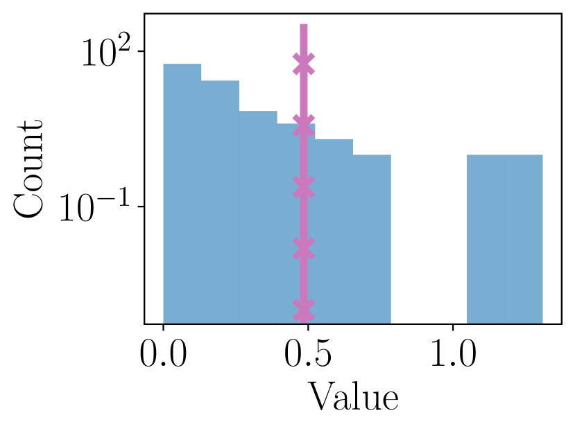
(a) log1
Logistic + L2
($\lambda=1\text{e-}3$)

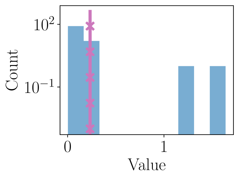
(b) log2
Logistic + L2
($\lambda=1\text{e-}3$)

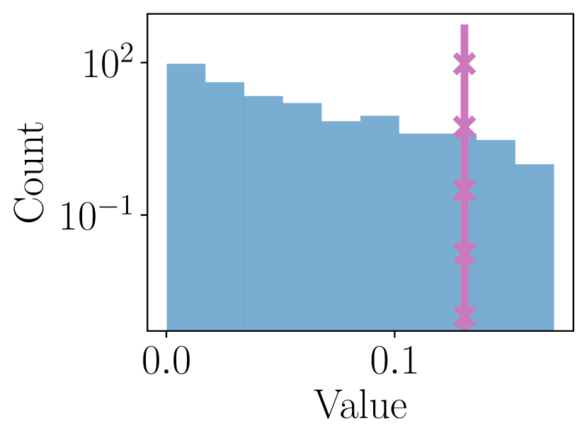
(c) mtp
Least Squares + L2
($\lambda=5\text{e-}8$)

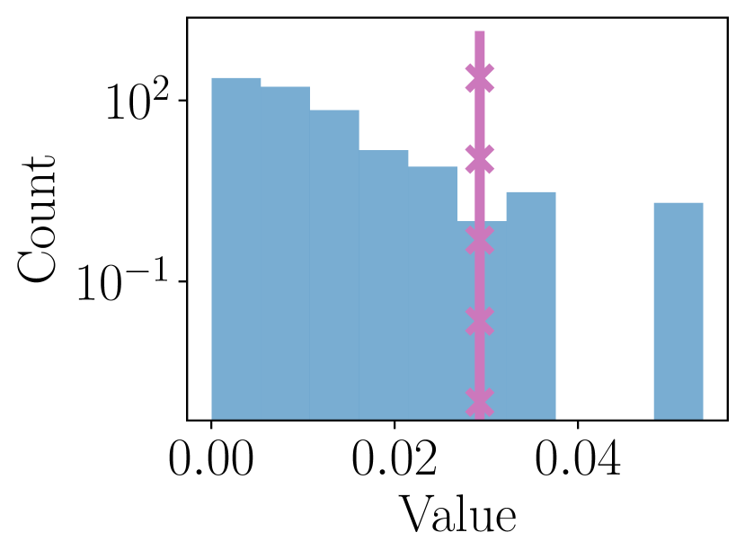
(d) madelon
Logistic + L2
($\lambda=1$)

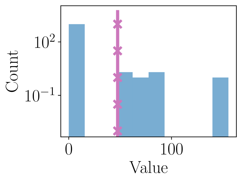
(e) square
LASSO
($\lambda=30$)

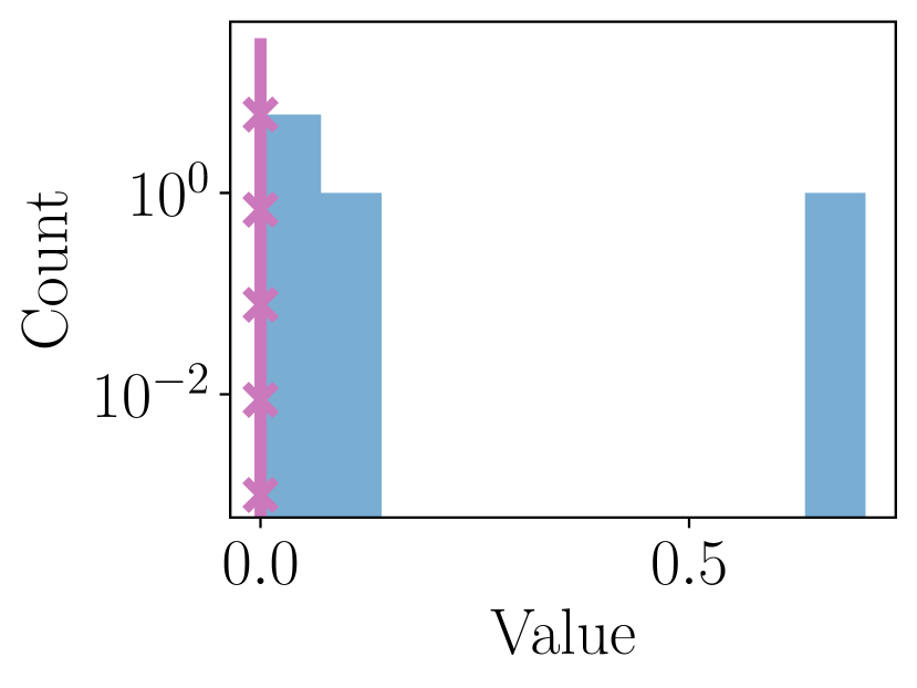
(f) california
LASSO
($\lambda=0.1$)

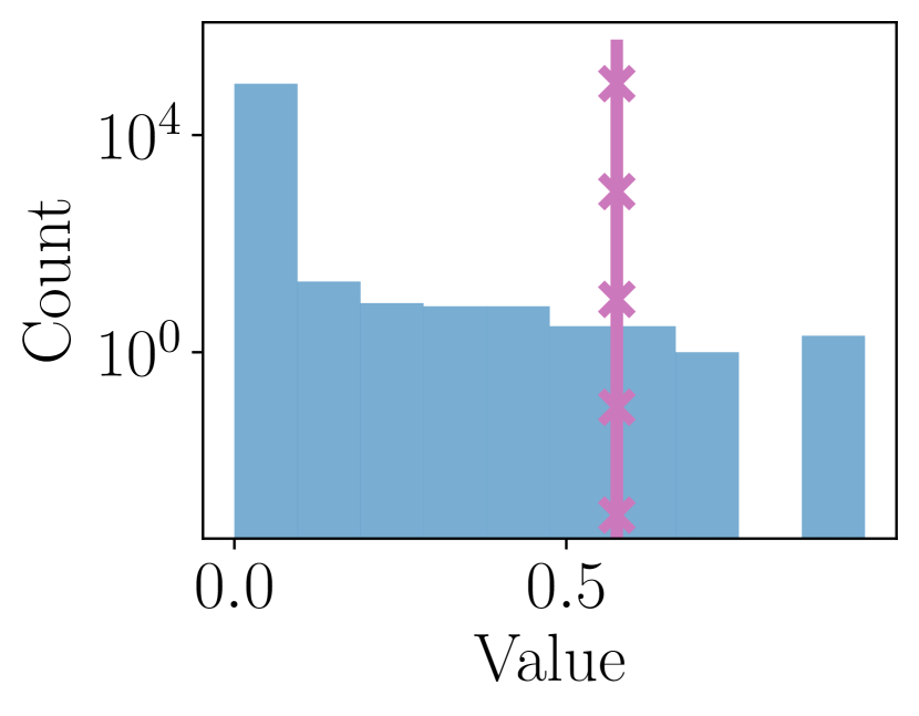
(g) dorothea
Logistic + L1
($\lambda=0.01$)

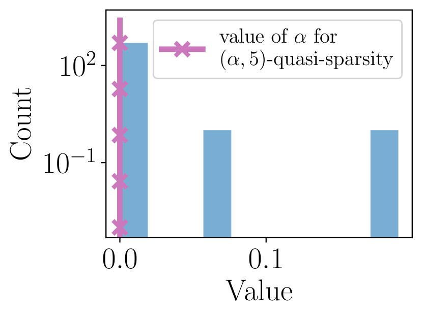
(h) madelon
Logistic + L1
($\lambda=0.05$)

Figure 2: Histograms of the absolute value of each problem solution’s parameters. Purple line indicates the $\alpha$ for which the plotted vector is $(\alpha,5)$-quasi-sparse. Y-axis is logarithmic.

Hyperparameters

On all datasets, we use the same hyperparameter grid. For each algorithm, we choose between roughly the same number of hyperparameters. The number of passes on data represents $p$ iterations of DP-CD, $n$ iterations of DP-SGD, and $1$ iteration of DP-GCD. The complete grid is described in Table 2, and the chosen hyperparameters for each problem and algorithm are given in Table 4.

Table 2: Hyperparameter grid used in our experiments.

Algorithm	Parameter	Values
	Passes on data	[0.001, 0.01, 0.1, 1, 2, 3, 5, 10, 20]
DP-CD	Step sizes	np.logspace(-2, 1, 10)
	Clipping threshold	np.logspace(-4, 6, 50)
	Passes on data	[0.001, 0.01, 0.1, 1, 2, 3, 5, 10, 20]
DP-SGD	Step sizes	np.logspace(-6, 0, 10)
	Clipping threshold	np.logspace(-4, 6, 50)
	Passes on data	[1, 2, 4, 7, 10, 15, 20]
DP-GCD	Step sizes	np.logspace(-2, 1, 10)
	Clipping threshold	np.logspace(-4, 6, 50)

Recovery of the support

In Table 3, we report the number of coordinates that are correctly/incorrectly identified as non-zero on $\ell_{1}$ regularized problems. Contrary to DP-SGD and DP-CD, DP-GCD never incorrectly identifies a coordinate as non-zero. Additionally, the suboptimality gap is lower for DP-GCD: its updates thus lead to better solutions.

Table 3: Coordinates correctly/incorrectly identified as non-zeros by each algorithm, and relative suboptimality gap $(f(w^{priv})-f^{*})/f^{*}$ (averaged over 5 runs).

	square	california	dorothea	madelon
$\|w^{*}\|_{0}$	7	3	72	3
DP-CD	0 / 0 (0.75)	3 / 2 (0.0024)	1 / 1 (0.77)	0 / 0 (0.0085)
DP-SGD	0 / 3 (0.75)	3 / 5 (0.020)	0 / 0 (0.78)	0 / 0 (0.012)
DP-GCD	2 / 0 (0.35)	2 / 0 (0.00056)	1 / 0 (0.64)	1 / 0 (0.0015)

Additional experiments on proximal DP-GCD

In Figure 3, we show the results of the proximal DP-GCD algorithm, after tuning the hyperparameters with the grid described above for each of the GS-s, GS-r and GS-q rules.

The three rules seem to behave qualitatively the same on square, dorothea and madelon, our three high-dimensional non-smooth problems. There, most coordinates are chosen about one time. Thus, as described by [27], all the steps are “good” steps (along their terminology): and on such good steps, the three rules coincide. On the lower-dimensional dataset california, coordinates can be chosen more than one time, and “bad” steps are likely to happen. On these steps, the three rules differ.

Runtime

Finally, we report the runtime of DP-GCD, in comparison with DP-CD and DP-SGD in Figure 4, that is the counterpart of Figure 1, except with runtime on the $x$-axis. These results confirm the fact that DP-GCD can be efficient, although its iterations are expensive to compute. Indeed, in imbalanced problems, the small number of iterations of DP-GCD enables it to run faster than DP-SGD, and in roughly the same time as DP-CD, while improving utility.

Table 4: Selected hyperparameters for every dataset and algorithm.

plots/best_params_treated.csv

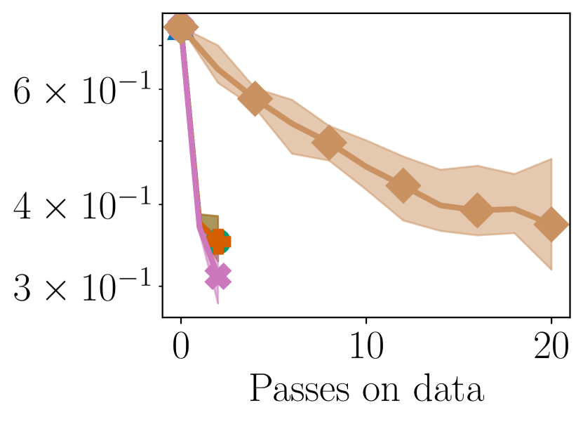
(a) sparse
LASSO
($\lambda=30$)

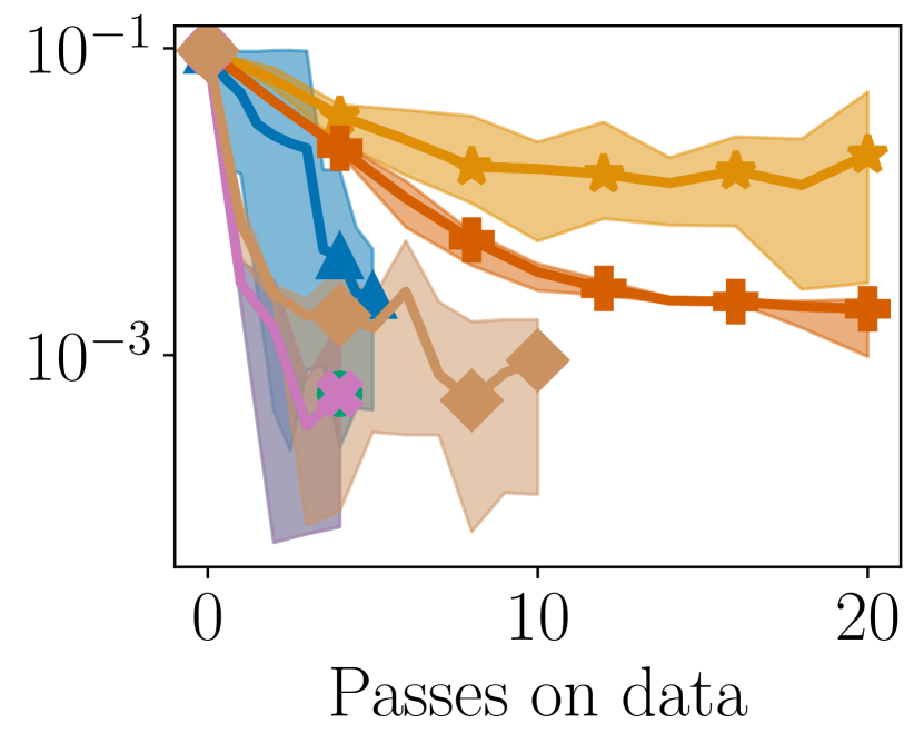
(b) california
LASSO
($\lambda=0.1$)

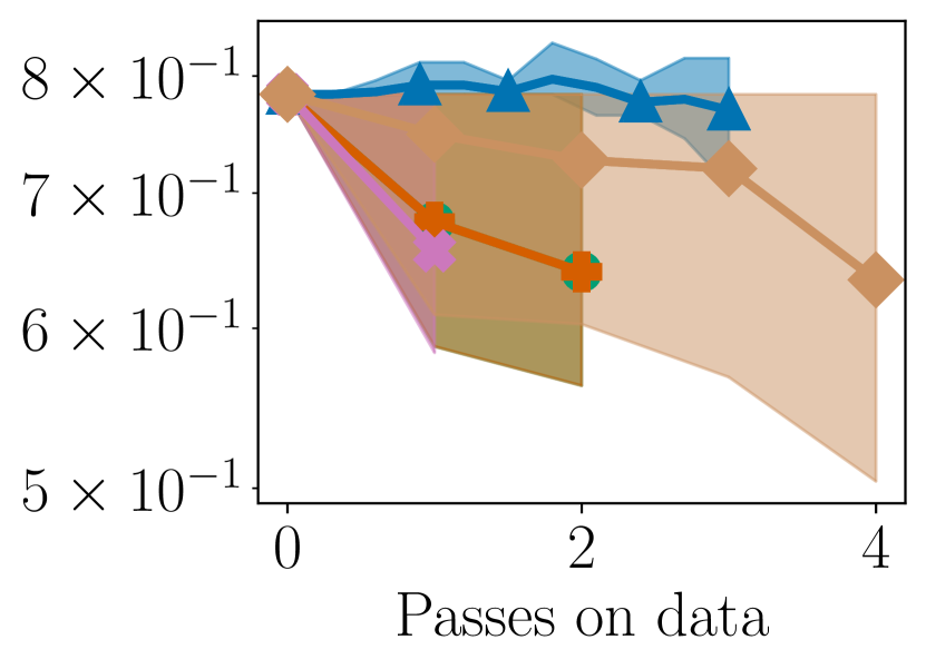
(c) dorothea
Logistic + L1
($\lambda=0.01$)

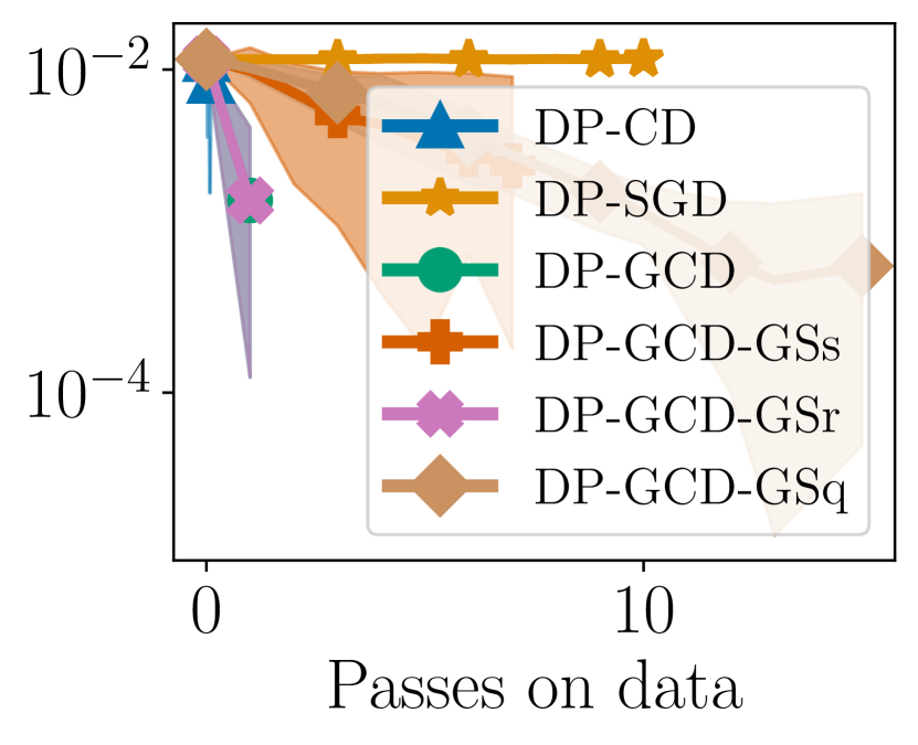
(d) madelon
Logistic + L1
($\lambda=0.05$)

Figure 3: Relative error to non-private optimal for DP-CD, proximal DP-GCD (with GS-r, GS-s and GS-q rules) and DP-SGD on different problems. On the x-axis, $1$ tick represents a full access to the data: $p$ iterations of DP-CD, $n$ iterations of DP-SGD and $1$ iteration of DP-GCD. Number of iterations, clipping thresholds and step sizes are tuned simultaneously for each algorithm. We report min/mean/max values over 5 runs.

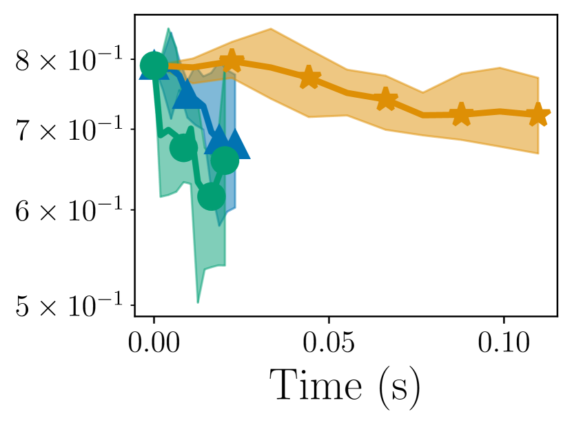
(a) log1
Logistic + L2
($\lambda=1\text{e-}3$)

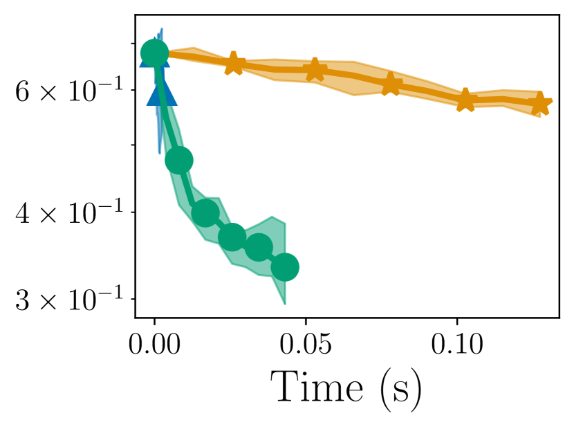
(b) log2
Logistic + L2
($\lambda=1\text{e-}3$)

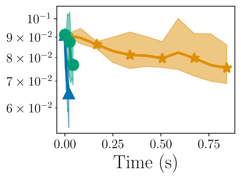
(c) mtp
Least Squares + L2
($\lambda=5\text{e-}8$)

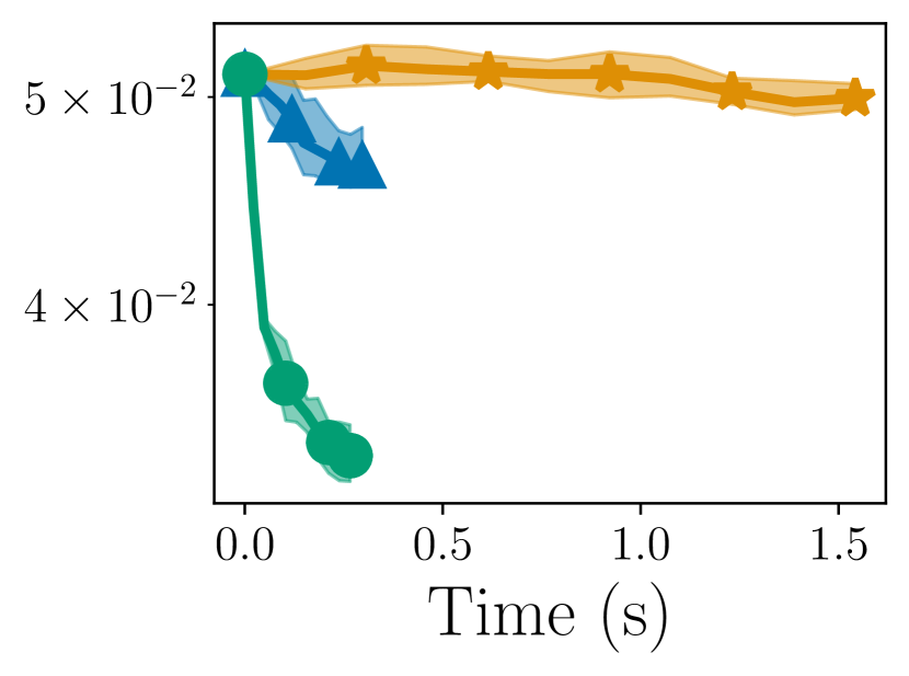
(d) madelon
Logistic + L2
($\lambda=1$)

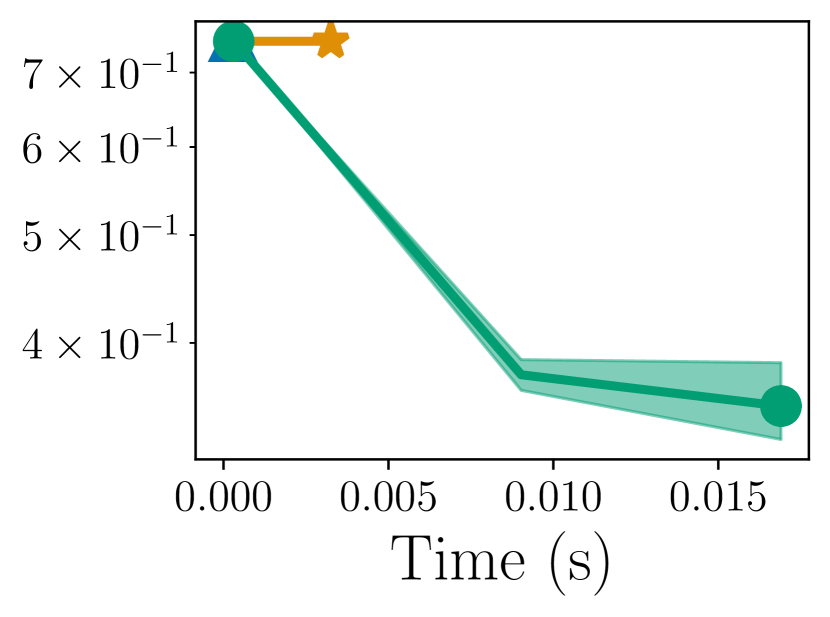
(e) sparse
LASSO
($\lambda=30$)

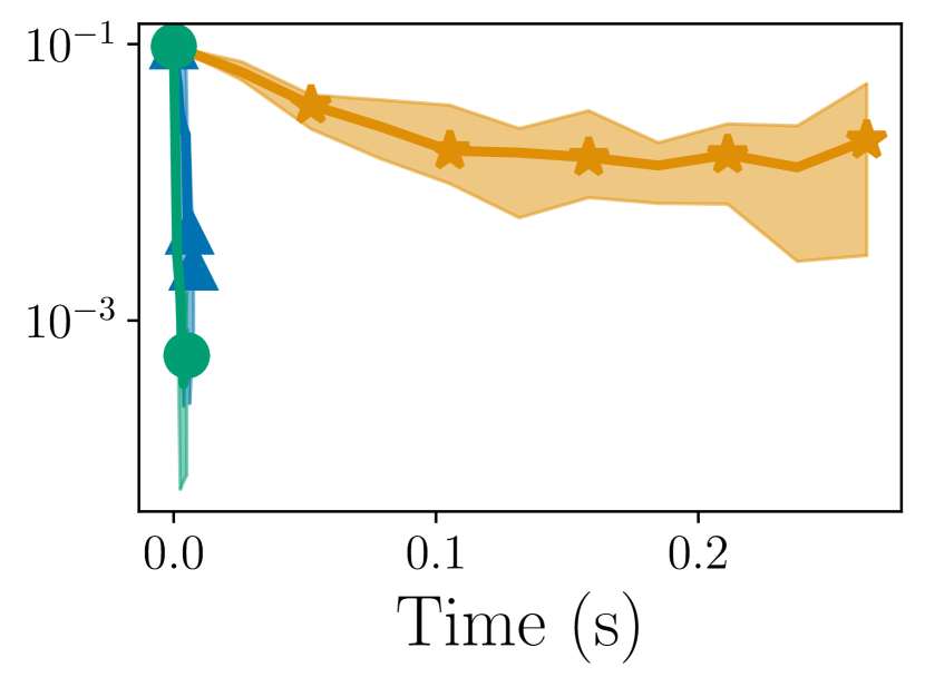
(f) california
LASSO
($\lambda=0.1$)

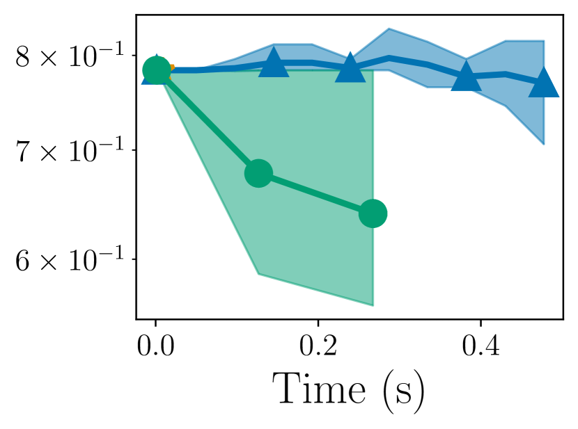
(g) dorothea
Logistic + L1
($\lambda=0.01$)

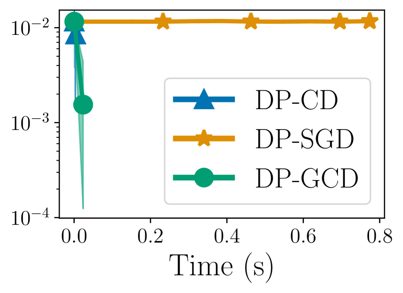
(h) madelon
Logistic + L1
($\lambda=0.05$)

Figure 4: Relative error to non-private optimal for DP-CD, DP-GCD and DP-SGD on different problems, as a function of running time. Number of iterations, clipping thresholds and step sizes are tuned simultaneously for each algorithm. We report min/mean/max values over 5 runs.

References

• [1] Martin Abadi, Andy Chu, Ian Goodfellow, H. McMahan, Ilya Mironov, Kunal Talwar and Li Zhang “Deep Learning with Differential Privacy” In Proceedings of the 2016 ACM SIGSAC Conference on Computer and Communications Security, CCS ’16 New York, NY, USA: Association for Computing Machinery, 2016, pp. 308–318 DOI: 10.1145/2976749.2978318
• [2] Hilal Asi, Vitaly Feldman, Tomer Koren and Kunal Talwar “Private Stochastic Convex Optimization: Optimal Rates in $\ell_{1}$ Geometry” In International Conference on Machine Learning PMLR, 2021 arXiv: http://arxiv.org/abs/2103.01516
• [3] Raef Bassily, Vitaly Feldman, Cristóbal Guzmán and Kunal Talwar “Stability of Stochastic Gradient Descent on Nonsmooth Convex Losses” In Advances in Neural Information Processing Systems 33 Curran Associates, Inc., 2020, pp. 4381–4391 URL: https://proceedings.neurips.cc/paper/2020/hash/2e2c4bf7ceaa4712a72dd5ee136dc9a8-Abstract.html
• [4] Raef Bassily, Vitaly Feldman, Kunal Talwar and Abhradeep Guha Thakurta “Private Stochastic Convex Optimization with Optimal Rates” In Advances in Neural Information Processing Systems 32 Curran Associates, Inc., 2019 URL: https://proceedings.neurips.cc/paper/2019/hash/3bd8fdb090f1f5eb66a00c84dbc5ad51-Abstract.html
• [5] Raef Bassily, Cristobal Guzman and Anupama Nandi “Non-Euclidean Differentially Private Stochastic Convex Optimization” In Proceedings of Thirty Fourth Conference on Learning Theory PMLR, 2021, pp. 474–499 URL: https://proceedings.mlr.press/v134/bassily21a.html
• [6] Raef Bassily, Kobbi Nissim, Adam Smith, Thomas Steinke, Uri Stemmer and Jonathan Ullman “Algorithmic Stability for Adaptive Data Analysis” In Proceedings of the Forty-Eighth Annual ACM Symposium on Theory of Computing, STOC ’16 New York, NY, USA: Association for Computing Machinery, 2016, pp. 1046–1059 DOI: 10.1145/2897518.2897566
• [7] Raef Bassily, Adam Smith and Abhradeep Thakurta “Differentially Private Empirical Risk Minimization: Efficient Algorithms and Tight Error Bounds” In arXiv:1405.7085 [cs, stat], 2014 arXiv: http://arxiv.org/abs/1405.7085
• [8] Aurélien Bellet, Rachid Guerraoui, Mahsa Taziki and Marc Tommasi “Personalized and Private Peer-to-Peer Machine Learning” In International Conference on Artificial Intelligence and Statistics PMLR, 2018, pp. 473–481 URL: http://proceedings.mlr.press/v84/bellet18a.html
• [9] Stephen P. Boyd and Lieven Vandenberghe “Convex Optimization” Cambridge, UK ; New York: Cambridge University Press, 2004
• [10] Kamalika Chaudhuri, Claire Monteleoni and Anand D. Sarwate “Differentially Private Empirical Risk Minimization” In Journal of Machine Learning Research 12.29, 2011, pp. 1069–1109 URL: http://jmlr.org/papers/v12/chaudhuri11a.html
• [11] Georgios Damaskinos, Celestine Mendler-Dünner, Rachid Guerraoui, Nikolaos Papandreou and Thomas Parnell “Differentially Private Stochastic Coordinate Descent” In Proceedings of the AAAI Conference on Artificial Intelligence 35, 2021, pp. 7176–7184 URL: https://ojs.aaai.org/index.php/AAAI/article/view/16882
• [12] Inderjit Dhillon, Pradeep Ravikumar and Ambuj Tewari “Nearest Neighbor Based Greedy Coordinate Descent” In Advances in Neural Information Processing Systems 24 Curran Associates, Inc., 2011 URL: https://papers.nips.cc/paper/2011/hash/160c88652d47d0be60bfbfed25111412-Abstract.html
• [13] Cynthia Dwork “Differential Privacy” In Automata, Languages and Programming, Lecture Notes in Computer Science Berlin, Heidelberg: Springer, 2006, pp. 1–12 DOI: 10.1007/11787006˙1
• [14] Cynthia Dwork, Vitaly Feldman, Moritz Hardt, Toniann Pitassi, Omer Reingold and Aaron Leon Roth “Preserving Statistical Validity in Adaptive Data Analysis” In Proceedings of the Forty-Seventh Annual ACM Symposium on Theory of Computing, STOC ’15 New York, NY, USA: Association for Computing Machinery, 2015, pp. 117–126 DOI: 10.1145/2746539.2746580
• [15] Cynthia Dwork and Aaron Roth “The Algorithmic Foundations of Differential Privacy” In Foundations and Trends® in Theoretical Computer Science 9.3-4, 2013, pp. 211–407 DOI: 10.1561/0400000042
• [16] Huang Fang, Zhenan Fan, Yifan Sun and Michael Friedlander “Greed Meets Sparsity: Understanding and Improving Greedy Coordinate Descent for Sparse Optimization” In Proceedings of the Twenty Third International Conference on Artificial Intelligence and Statistics PMLR, 2020, pp. 434–444 URL: https://proceedings.mlr.press/v108/fang20a.html
• [17] Vitaly Feldman, Tomer Koren and Kunal Talwar “Private Stochastic Convex Optimization: Optimal Rates in Linear Time” In Proceedings of the 52nd Annual ACM SIGACT Symposium on Theory of Computing New York, NY, USA: Association for Computing Machinery, 2020, pp. 439–449 URL: https://doi.org/10.1145/3357713.3384335
• [18] Olivier Fercoq and Peter Richtárik “Accelerated, Parallel and Proximal Coordinate Descent” In arXiv:1312.5799 [cs, math, stat], 2014 arXiv: http://arxiv.org/abs/1312.5799
• [19] Marguerite Frank and Philip Wolfe “An Algorithm for Quadratic Programming” In Naval Research Logistics Quarterly 3.1-2, 1956, pp. 95–110 DOI: 10.1002/nav.3800030109
• [20] Filip Hanzely, Konstantin Mishchenko and Peter Richtarik “SEGA: Variance Reduction via Gradient Sketching” In Proceedings of the 32nd International Conference on Neural Information Processing Systems, NIPS’18 Red Hook, NY, USA: Curran Associates Inc., 2018, pp. 2086–2097
• [21] Moritz Hardt, Ben Recht and Yoram Singer “Train Faster, Generalize Better: Stability of Stochastic Gradient Descent” In Proceedings of The 33rd International Conference on Machine Learning PMLR, 2016, pp. 1225–1234 URL: https://proceedings.mlr.press/v48/hardt16.html
• [22] Lijie Hu, Shuo Ni, Hanshen Xiao and Di Wang “High Dimensional Differentially Private Stochastic Optimization with Heavy-tailed Data” In Proceedings of the 41st ACM SIGMOD-SIGACT-SIGAI Symposium on Principles of Database Systems, PODS ’22 New York, NY, USA: Association for Computing Machinery, 2022, pp. 227–236 DOI: 10.1145/3517804.3524144
• [23] Martin Jaggi “Revisiting Frank-Wolfe: Projection-Free Sparse Convex Optimization” In International Conference on Machine Learning PMLR, 2013, pp. 427–435 URL: http://proceedings.mlr.press/v28/jaggi13.html
• [24] Rie Johnson and Tong Zhang “Accelerating Stochastic Gradient Descent Using Predictive Variance Reduction” In Advances in Neural Information Processing Systems 26 Curran Associates, Inc., 2013 URL: https://proceedings.neurips.cc/paper/2013/file/ac1dd209cbcc5e5d1c6e28598e8cbbe8-Paper.pdf
• [25] Christopher Jung, Katrina Ligett, Seth Neel, Aaron Roth, Saeed Sharifi-Malvajerdi and Moshe Shenfeld “A New Analysis of Differential Privacy&#x2019;s Generalization Guarantees (Invited Paper)” In Proceedings of the 53rd Annual ACM SIGACT Symposium on Theory of Computing New York, NY, USA: Association for Computing Machinery, 2021, pp. 9 URL: https://doi.org/10.1145/3406325.3465358
• [26] Peter Kairouz, Monica Ribero Diaz, Keith Rush and Abhradeep Thakurta “(Nearly) Dimension Independent Private ERM with AdaGrad Rates via Publicly Estimated Subspaces” In Proceedings of Thirty Fourth Conference on Learning Theory PMLR, 2021, pp. 2717–2746 URL: https://proceedings.mlr.press/v134/kairouz21a.html
• [27] Sai Praneeth Karimireddy, Anastasia Koloskova, Sebastian U. Stich and Martin Jaggi “Efficient Greedy Coordinate Descent for Composite Problems” In The 22nd International Conference on Artificial Intelligence and Statistics PMLR, 2019, pp. 2887–2896 URL: http://proceedings.mlr.press/v89/karimireddy19a.html
• [28] Shiva Prasad Kasiviswanathan and Hongxia Jin “Efficient Private Empirical Risk Minimization for High-dimensional Learning”, 2016, pp. 10
• [29] Daniel Kifer, Adam Smith and Abhradeep Thakurta “Private Convex Empirical Risk Minimization and High-dimensional Regression”, 2012, pp. 40
• [30] Zhi-Quan Luo and Paul Tseng “On the Convergence of the Coordinate Descent Method for Convex Differentiable Minimization” In Journal of Optimization Theory and Applications 72.1, 1992, pp. 7–35 DOI: 10.1007/BF00939948
• [31] Paul Mangold, Aurélien Bellet, Joseph Salmon and Marc Tommasi “Differentially Private Coordinate Descent for Composite Empirical Risk Minimization” In International Conference on Machine Learning PMLR, 2022 arXiv: http://arxiv.org/abs/2110.11688
• [32] M. Massias, A. Gramfort and J. Salmon “From safe screening rules to working sets for faster Lasso-type solvers” In NIPS-OPT, 2017
• [33] Ilya Mironov “Renyi Differential Privacy” In 2017 IEEE 30th Computer Security Foundations Symposium (CSF), 2017, pp. 263–275 DOI: 10.1109/CSF.2017.11
• [34] Ilya Mironov, Kunal Talwar and Li Zhang “Rényi Differential Privacy of the Sampled Gaussian Mechanism” In arXiv:1908.10530 [cs, stat], 2019 arXiv: http://arxiv.org/abs/1908.10530
• [35] Yu. Nesterov “Efficiency of Coordinate Descent Methods on Huge-Scale Optimization Problems” In SIAM Journal on Optimization 22.2, 2012, pp. 341–362 DOI: 10.1137/100802001
• [36] Julie Nutini, Mark Schmidt, Issam Laradji, Michael Friedlander and Hoyt Koepke “Coordinate Descent Converges Faster with the Gauss-Southwell Rule Than Random Selection” In International Conference on Machine Learning PMLR, 2015, pp. 1632–1641 URL: http://proceedings.mlr.press/v37/nutini15.html
• [37] Neal Parikh and Stephen Boyd “Proximal Algorithms” In Foundations and Trends in Optimization 1.3, 2014, pp. 127–239 DOI: 10.1561/2400000003
• [38] Fabian Pedregosa, Gael Varoquaux, Alexandre Gramfort, Vincent Michel, Bertrand Thirion, Olivier Grisel, Mathieu Blondel, Peter Prettenhofer, Ron Weiss, Vincent Dubourg, Jake Vanderplas, Alexandre Passos and David Cournapeau “Scikit-Learn: Machine Learning in Python” In MACHINE LEARNING IN PYTHON, 2011, pp. 6
• [39] Peter Richtárik and Martin Takáč “Iteration Complexity of Randomized Block-Coordinate Descent Methods for Minimizing a Composite Function” In Mathematical Programming 144.1-2, 2014, pp. 1–38 DOI: 10.1007/s10107-012-0614-z
• [40] Shai Shalev-Shwartz and Tong Zhang “Stochastic Dual Coordinate Ascent Methods for Regularized Loss” In The Journal of Machine Learning Research 14.1, 2013, pp. 567–599 URL: https://dl.acm.org/doi/10.5555/2567709.2502598
• [41] Hao-Jun Michael Shi, Shenyinying Tu, Yangyang Xu and Wotao Yin “A Primer on Coordinate Descent Algorithms” In arXiv:1610.00040 [math, stat], 2017 arXiv: http://arxiv.org/abs/1610.00040
• [42] Reza Shokri, Marco Stronati, Congzheng Song and Vitaly Shmatikov “Membership Inference Attacks Against Machine Learning Models” In 2017 IEEE Symposium on Security and Privacy (SP), 2017, pp. 3–18 DOI: 10.1109/SP.2017.41
• [43] Sebastian U. Stich, Anant Raj and Martin Jaggi “Approximate Steepest Coordinate Descent” In Proceedings of the 34th International Conference on Machine Learning PMLR, 2017, pp. 3251–3259 URL: https://proceedings.mlr.press/v70/stich17a.html
• [44] Kunal Talwar, Abhradeep Guha Thakurta and Li Zhang “Nearly Optimal Private LASSO” In Advances in Neural Information Processing Systems 28, 2015 URL: https://proceedings.neurips.cc/paper/2015/hash/52d080a3e172c33fd6886a37e7288491-Abstract.html
• [45] Kunal Talwar, Abhradeep Thakurta and Li Zhang “Private Empirical Risk Minimization Beyond the Worst Case: The Effect of the Constraint Set Geometry” arXiv: 1411.5417 In arXiv:1411.5417 [cs, stat], 2016 URL: http://arxiv.org/abs/1411.5417
• [46] Rachael Tappenden, Peter Richtárik and Jacek Gondzio “Inexact Coordinate Descent: Complexity and Preconditioning” In Journal of Optimization Theory and Applications 170.1, 2016, pp. 144–176 DOI: 10.1007/s10957-016-0867-4
• [47] Robert Tibshirani “Regression Shrinkage and Selection Via the Lasso” In Journal of the Royal Statistical Society: Series B (Methodological) 58.1, 1996, pp. 267–288 DOI: 10.1111/j.2517-6161.1996.tb02080.x
• [48] Paul Tseng “Convergence of a Block Coordinate Descent Method for Nondifferentiable Minimization” In Journal of Optimization Theory and Applications 109.3, 2001, pp. 475–494 DOI: 10.1023/A:1017501703105
• [49] Paul Tseng and Sangwoon Yun “A Coordinate Gradient Descent Method for Nonsmooth Separable Minimization” In Mathematical Programming 117.1, 2009, pp. 387–423 DOI: 10.1007/s10107-007-0170-0
• [50] Joaquin Vanschoren, Jan N. rijnvan Rijn, Bernd Bischl and Luis Torgo “OpenML: Networked Science in Machine Learning” In ACM SIGKDD Explorations Newsletter 15.2, 2014, pp. 49–60 DOI: 10.1145/2641190.2641198
• [51] Di Wang, Minwei Ye and Jinhui Xu “Differentially Private Empirical Risk Minimization Revisited: Faster and More General” In Advances in Neural Information Processing Systems 30 Curran Associates, Inc., 2017 URL: https://proceedings.neurips.cc/paper/2017/file/f337d999d9ad116a7b4f3d409fcc6480-Paper.pdf
• [52] Lingxiao Wang and Quanquan Gu “Differentially private iterative gradient hard thresholding for sparse learning” In Proceedings of the 28th International Joint Conference on Artificial Intelligence, IJCAI’19 Macao, China: AAAI Press, 2019, pp. 3740–3747
• [53] Puyu Wang, Yunwen Lei, Yiming Ying and Hai Zhang “Differentially Private SGD with Non-Smooth Losses” In Applied and Computational Harmonic Analysis 56, 2022, pp. 306–336 DOI: 10.1016/j.acha.2021.09.001
• [54] Stephen J. Wright “Coordinate Descent Algorithms” In Mathematical Programming 151.1, 2015, pp. 3–34 DOI: 10.1007/s10107-015-0892-3
• [55] Xi Wu, Fengan Li, Arun Kumar, Kamalika Chaudhuri, Somesh Jha and Jeffrey Naughton “Bolt-on Differential Privacy for Scalable Stochastic Gradient Descent-based Analytics” In Proceedings of the 2017 ACM International Conference on Management of Data, SIGMOD ’17 New York, NY, USA: Association for Computing Machinery, 2017, pp. 1307–1322 DOI: 10.1145/3035918.3064047
• [56] Lin Xiao and Tong Zhang “A Proximal Stochastic Gradient Method with Progressive Variance Reduction” In SIAM Journal on Optimization 24.4 Society for Industrial and Applied Mathematics, 2014, pp. 2057–2075 DOI: 10.1137/140961791
• [57] Yingxue Zhou, Zhiwei Steven Wu and Arindam Banerjee “Bypassing the Ambiant Dimension: Private SGD with Gradient Subspace Identification”, 2021, pp. 28