Orthogonal decomposition of anisotropic constitutive models for the phase field approach to fracture

Abstract

We propose a decomposition of constitutive relations into crack-driving and persistent portions, specifically designed for materials with anisotropic/orthotropic behavior in the phase field approach to fracture to account for the tension-compression asymmetry. This decomposition follows a variational framework, satisfying the orthogonality condition for anisotropic materials. This implies that the present model can be applied to arbitrary anisotropic elastic behavior in a three-dimensional setting. On this basis, we generalize two existing models for tension-compression asymmetry in isotropic materials, namely the ‘volumetric-deviatoric’ model [5] and the ‘no-tension’ model [22], towards materials with anisotropic nature. Two benchmark problems, single notched tensile shear tests, are used to study the performance of the present model. The results can retain the anisotropic constitutive behavior and the tension-compression asymmetry in the crack response, and are qualitatively in accordance with the expected behavior for orthotropic materials. Furthermore, to study the direction of maximum energy dissipation, we modify the surface integral based energy release computation, $G_{\theta}$, to account only for the crack-driving energy. The computed energies with our proposed modifications predict the fracture propagation direction correctly compared with the standard $G_{\theta}$ method.

1 Introduction

The phase field method has steadily gained popularity for over a decade because of its convenience in simulating complex fracture processes, including crack nucleation, propagation, branching and merging [13]. The model was originally conceived as the variational formulation of brittle fracture by Francfort and Marigo [21], and its regularization by Bourdin et al [12]. The formulation solves crack problems by minimizing an energy functional that consists of the elastic energy and the crack surface energy. This significantly reduces the implementation complexities as the crack evolution is a natural outcome of the solution. Therefore, there is no need for a crack tracking algorithm or additional criteria for crack branching and merging. The method has found its extension in subjects such as composite failure [6, 1, 58], ductility [2, 4, 28, 36, 60], dynamic fracture [14, 10, 41, 57], hydraulic fracture [11, 54, 55, 26, 61], and environment assisted failure [35, 48] to name a few.
When mechanics of natural materials is concerned, especially geomaterials, they often exhibit anisotropic behaviors [16, 3, 44]. Anisotropic material response manifests itself in terms of deformation [42, 27] and/or preferential fracture propagation [53, 31]. In modeling anisotropy within the phase field framework, anisotropic fracture toughness has been mostly achieved through manipulation of the fracture surface energy term where one applies structural tensors [30, 50, 9, 29, 7, 23] or assign direction dependent fracture toughness [15, 43, 20, 46, 23, 51] to encourage fracture propagation in certain directions. While many studies are available for anisotropic fracture toughness, only a few have studied anisotropic constitutive model in phase field approaches [40, 52, 33].
Another material response to consider is tension-compression asymmetry in failure, i.e., a crack is less likely to propagate under compressive loadings. Consequently, there has to be a unilateral constraint in material degradation. Otherwise, unphysical crack propagation is predicted under compressive loading. How to account for this unilateral constraint is one of the main challenges in phase field modeling. Note that such a model is sometimes referred to in the literature as an ‘anisotropic’ phase field model [4], however, in this work we use the term of ‘tension-compression asymmetry’ for this effect (see also [39]), and preserve ‘anisotropy’ to only address a material whose constitutive behavior is, unlike isotropic materials, directionally dependent.
With the need of tension-compression asymmetry in material degradation, several existing approaches consist of additively partitioning the sound elastic energy density $\varPsi$ into two portions, a crack-driving portion $\varPsi^{\text{t}}$ and a persistent portion $\varPsi^{\text{c}}$ [5, 38, 22, 49, 56, 18]. If we are able to partition the strain energy density based on the additive decomposition of the strain tensor, that is,

$$\bm{\varepsilon}=\bm{\varepsilon}^{\text{t}}+\bm{\varepsilon}^{\text{c}},\quad\varPsi(\bm{\varepsilon})=\varPsi^{\text{t}}(\bm{\varepsilon}^{\text{t}})+\varPsi^{\text{c}}(\bm{\varepsilon}^{\text{c}}),$$

$$\varPsi^{\text{t}}(\bm{\varepsilon}^{\text{t}})=\frac{1}{2}\mathbb{C}\bm{\varepsilon}^{\text{t}}\cdot\bm{\varepsilon}^{\text{t}},\quad\varPsi^{\text{c}}(\bm{\varepsilon}^{\text{t}})=\frac{1}{2}\mathbb{C}\bm{\varepsilon}^{\text{c}}\cdot\bm{\varepsilon}^{\text{c}},$$

the constitutive behaviors are characterized by the same elasticity tensor $\mathbb{C}$ where a dot $\cdot$ denotes the inner products between the two vectors or tensors of the same order. Then, there exists a local variational principle from which several existing models can be derived:

$$\bm{\varepsilon}^{\text{t}}=\underset{\bm{e}^{\text{t}}\in\mathcal{S}^{\text{t}}}{\mathrm{argmin}}\,\mathbb{C}\bigl{(}\bm{\varepsilon}-\bm{e}^{\text{t}}\bigr{)}\cdot\bigl{(}\bm{\varepsilon}-\bm{e}^{\text{t}}\bigr{)},$$ (1)

where the strain that contributes to damage ($\bm{\varepsilon}^{\text{t}}$) is defined as the orthogonal projection of the strain tensor $\bm{\varepsilon}$ onto the convex space $\mathcal{S}^{\text{t}}$ with respect to the energy norm defined by $\mathbb{C}$. Therefore, the modeling of tension-compression asymmetry in fracture response is reduced to the identification of such convex cone $\mathcal{S}^{\text{t}}$ to represent $\bm{\varepsilon}^{\text{t}}$ [22]. Also, $\bm{\varepsilon}^{\text{c}}$ is in a polar cone $\mathcal{S}^{\text{c}}=\Big{\{}\bm{e}^{\text{c}}\Big{|}\bm{e}^{\text{c}}\cdot\bm{e}^{\text{t}}\leq 0,~{}\forall\bm{e}^{\text{t}}\in\mathcal{S}^{\text{t}}\Big{\}}$. This way, we keep the variational structure of the crack problem by following the energy minimization. This is important because otherwise, one needs to introduce ad hoc criteria for the phase field problem. For more detailed analysis, we refer the readers to [34] and [22].
A challenges in anisotropic materials is to satisfy this variational structure. From convex analysis, $\bm{\varepsilon}^{\text{t}}$ can be equivalently characterized by

$$-\mathbb{C}(\bm{\varepsilon}-\bm{\varepsilon}^{\text{t}})\cdot\bigl{(}\bm{e}^{\text{t}}-\bm{\varepsilon}^{\text{t}}\bigr{)}\geq 0,\quad\forall\bm{e}^{\text{t}}\in\mathcal{S}^{\text{t}}.$$

Testing this with $\bm{e}^{\text{t}}=2\bm{\varepsilon}^{\text{t}}$ and $\bm{e}^{\text{t}}=\frac{1}{2}\bm{\varepsilon}^{\text{t}}$ yields the following orthogonality condition [32]:

$$\mathbb{C}\bm{\varepsilon}^{\text{t}}\cdot\bm{\varepsilon}^{\text{c}}=\mathbb{C}\bm{\varepsilon}^{\text{c}}\cdot\bm{\varepsilon}^{\text{t}}=0,$$ (2)

which is the necessary and sufficient condition for the strain energy density to be decomposed based on the partition of the strain tensor. However, for anisotropic linear elastic materials the principal directions of the stress and strain no longer coincide, i.e., the orthogonality condition is not generally satisfied:

$$\mathbb{C}\bm{\varepsilon}^{\text{t}}\cdot\bm{\varepsilon}^{\text{c}}\neq 0\text{~{}or~{}}\mathbb{C}\bm{\varepsilon}^{\text{c}}\cdot\bm{\varepsilon}^{\text{t}}\neq 0.$$

Therefore, further treatments are required in strain decomposition that keep the orthogonality condition for anisotropic materials.
Recently, He and Shao [25] proposed an elastic energy preserving transformation so that an orthogonal decomposition of the strain tensor can be achieved in the transformed space. Therein, a rigorously orthogonal spectral decomposition of the strain tensor is performed. Thus, with the orthogonality condition being satisfied in the new space, the strain energy density of an anisotropic material is respectively partitioned into a crack-driving portion and a persistent portion. Moreover, to decompose the strain tensor in a two-dimensional setting, a set of closed-form coordinate-free expressions are provided. Nguyen et al. [40] directly employed these expressions of strain decomposition into the phase field formulation, and compared the results with volumetric-deviatoric and spectral-decomposition for isotropic materials. Van Dijk et al. [52] proposed a generalization of volumetric-deviatoric and spectral-decomposition to account for anisotropy of materials. Therein, the strain energy density is described as an isotropic tensor function of a type of tensorial square roots of the strain energy density.
In this work, we present generalized formulations of two existing models for tension-compression asymmetry, a model by Amor et al. [5] (henceforth referred to as volumetric-deviatoric) and a model by Freddi and Royer [22] (henceforth referred to as no-tension), to account for materials with anisotropic constitutive behavior in a three-dimensional setting. We borrow the basic concepts from [25] and perform the energy preserving transformation so that the orthogonality condition is preserved for a decomposition of an arbitrary anisotropic constitutive model. Then, we present the implementation details of volumetric-deviatoric and no-tension accounting for the anisotropy in Section 2. In addition, we provide a set of numerical examples to illustrate the capabilities of the present method in Section 3. The results provide a step forward when developing phase field fracture theories for brittle materials with an anisotropic nature and highlight the importance of a proper decomposition of the strain energy density.

2 Problem statement

This section introduces the theory and implementation details to account for the tension-compression asymmetry in the crack response of anisotropic materials. In 2.1 we recapitulate the basic ingredients of a phase field formulation. Then, in 2.2 we perform an elastic energy preserving transformation so that an orthogonal decomposition of the strain tensor, and its consequent partitioning of the strain energy density, can be realized in the transformed space. Thereafter, in 2.3 we pick the two existing models for the tension-compression asymmetry, volumetric-deviatoric and no-tension, and adapt them for anisotropic materials. Finally, in 2.4 we provide various types of the elasticity tensors that can be adapted into the model. Readers interested in directly using the model can jump to (19), (20), (21), (22) for anisotropic volumetric-deviatoric and (26), (27), (29), (31) for anisotropic no-tension.

2.1 Phase field formulation

The phase field formulation for brittle fracture is essentially based on minimization of the following functional

$$\Pi_{\ell}(\bm{u},d):=\int_{\Omega}\varPsi\bigl{[}\bm{\varepsilon}(\bm{u}),d\bigr{]}\,\mathrm{d}\Omega-\int_{\partial\Omega_{t}}\bm{t}_{N}\cdot\bm{u}\,\mathrm{d}A-\int_{\Omega}\bm{b}\cdot\bm{u}\,\mathrm{d}\Omega+\int_{\Omega}G_{c}\gamma(d,\nabla d)~{}\mathrm{d}\Omega,$$ (3)

where $d:\Omega\rightarrow[0,1]$ represents the phase field, characterizing the material at its pristine state with $d=0$ and at the fully damaged state with $d=1$. Also, $\bm{t}_{N}:\partial\Omega_{t}\rightarrow\mathbb{R}^{n}$ is the prescribed traction boundary condition, and $\bm{b}:\Omega\rightarrow\mathbb{R}^{n}$ is the body force. The strain energy density takes the following form

$$\varPsi\bigl{[}\bm{\varepsilon},d\bigr{]}=g(d)\varPsi^{\text{t}}(\bm{\varepsilon}^{\text{t}})+\varPsi^{\text{c}}(\bm{\varepsilon}^{\text{c}}),$$ (4)

where $g(d)=(1-d)^{2}$ is a degradation function. Furthermore, $G_{c}>0$ is the critical crack energy release rate, and $\gamma(d,\nabla d)$ is the crack surface density per unit volume,

$$\gamma(d,\nabla d)=\frac{1}{4c_{w}}\left(\frac{w(d)}{\ell}+\ell|\nabla d|^{2}\right),$$

where $\ell>0$ is the regularization length scale parameter which controls the width of the transition region of the smoothed crack. Crack geometric function $w(d)$ and normalization constant $c_{w}=\int_{0}^{1}\sqrt{w(d)}\,\mathrm{d}d$ are model dependent. Specifically, for brittle fracture, classical examples are $w(d)=d^{2}$ and $c_{w}=1/2$ for the AT₂ model; and $w(d)=d$ and $c_{w}=2/3$ for the AT₁ model [45].
In the sequel we derive the first and second variations of $\Pi_{\ell}$ as in (3), which will be needed for the discretized formulation.

First variation of $\Pi_{\ell}$

Taking the first variation yields:

$$\delta\Pi[(\bm{u},d);(\bar{\bm{u}},\bar{d})] :=\int_{\Omega}\bm{\sigma}\bigl{[}\bm{\varepsilon}(\bm{u}),d\bigr{]}\cdot\bm{\varepsilon}(\bar{\bm{u}})\,\mathrm{d}\Omega-\int_{\partial\Omega_{t}}\bm{t}_{N}\cdot\bar{\bm{u}}\,\mathrm{d}A-\int_{\Omega}\bm{b}\cdot\bar{\bm{u}}\,\mathrm{d}\Omega$$ (5)

$$+\int_{\Omega}g^{\prime}(d)\varPsi^{\text{t}}(\bm{\varepsilon})\bar{d}~{}\mathrm{d}\Omega+\frac{G_{c}}{4c_{w}}\int_{\Omega}\Bigl{(}\frac{w^{\prime}(d)\bar{d}}{\ell}+2\ell\nabla d\cdot\nabla\bar{d}\Bigr{)}~{}\mathrm{d}\Omega,$$

where

$$\bm{\sigma}:=\frac{\partial\varPsi}{\partial\bm{\varepsilon}}=g(d)\bm{\sigma}^{\text{t}}+\bm{\sigma}^{\text{c}},\quad\bm{\sigma}^{\text{t}}=\frac{\partial\varPsi^{\text{t}}}{\partial\bm{\varepsilon}},\quad\bm{\sigma}^{\text{c}}=\frac{\partial\varPsi^{\text{c}}}{\partial\bm{\varepsilon}}.$$ (6)

Second variation of $\Pi_{\ell}$

We take another variation from (3):

$$\delta^{2}\Pi[(\bm{u},d);(\bar{\bm{u}},\bar{d});(\delta\bm{u},\delta d)] :=\int_{\Omega}\bm{\varepsilon}(\delta\bm{u})\cdot\mathbb{C}\bigl{[}\bm{\varepsilon}(\bm{u}),d\bigr{]}\cdot\bm{\varepsilon}(\bar{\bm{u}})\,\mathrm{d}\Omega+\int_{\Omega}\bm{\varepsilon}(\delta\bm{u})\cdot\bm{\sigma}^{\text{t}}\bigl{[}\bm{\varepsilon}(\bm{u})\bigr{]}g^{\prime}(d)\bar{d}\,\mathrm{d}\Omega$$ (7)

$$+\int_{\Omega}\delta dg^{\prime}(d)\bm{\sigma}^{\text{t}}\bigl{[}\bm{\varepsilon}(\bm{u})\bigr{]}\cdot\bm{\varepsilon}(\bar{\bm{u}})\,\mathrm{d}\Omega+\int_{\Omega}\delta dg^{\prime\prime}(d)\varPsi^{\text{t}}(\bm{\varepsilon})\bar{d}\,\mathrm{d}\Omega$$

$$+\frac{g_{c}}{4c_{w}}\int_{\Omega}\Biggl{(}\frac{\delta dw^{\prime\prime}(d)\bar{d}}{\ell}+2\ell\nabla(\delta d)\cdot\nabla\bar{d}\Biggr{)}\,\mathrm{d}\Omega,$$

where

$$\mathbb{C}:=\frac{\partial^{2}\varPsi}{\partial\bm{\varepsilon}^{2}}=g(d)\mathbb{C}^{\text{t}}+\mathbb{C}^{\text{c}},\quad\mathbb{C}^{\text{t}}=\frac{\partial^{2}\varPsi^{\text{t}}}{\partial\bm{\varepsilon}^{2}},\quad\mathbb{C}^{\text{c}}=\frac{\partial^{2}\varPsi^{\text{c}}}{\partial\bm{\varepsilon}^{2}}.$$ (8)

The components of (4), (6), (8) are particularly obtained in the sequel.

2.2 Transformation for anisotropic $\mathbb{C}$

Let $\mathcal{S}$ and $\mathcal{S}^{*}$ be the set of all second-order strain and stress tensors, respectively. To enforce the orthogonality condition (2) for an arbitrary anisotropic $\mathbb{C}$, following He and Shao [25], we define the transformed strain and stress spaces as

$$\tilde{\mathcal{S}}=\Big{\{}\tilde{\bm{\varepsilon}}\Big{|}\tilde{\bm{\varepsilon}}=\mathbb{C}^{1/2}\bm{\varepsilon},~{}\bm{\varepsilon}\in\mathcal{S}\Big{\}},$$ (9a)

$${\tilde{\mathcal{S}}}^{*}=\Big{\{}\tilde{\bm{\sigma}}\Big{|}\tilde{\bm{\sigma}}=\mathbb{S}^{1/2}\bm{\sigma},~{}\bm{\sigma}\in\mathcal{S}^{*}\Big{\}},$$ (9b)

so that

$$\varPsi(\bm{\varepsilon})=\frac{1}{2}\tilde{\bm{\varepsilon}}\cdot\tilde{\bm{\varepsilon}}=\frac{1}{2}\tilde{\bm{\sigma}}\cdot\tilde{\bm{\sigma}}.$$ (10)

Note that $\mathbb{C}^{1/2}$ in (9a) is the square root of $\mathbb{C}$, and $\mathbb{S}^{1/2}$ in (9b) is the square root of the compliance tensor $\mathbb{S}=\mathbb{C}^{-1}$, see Remark (1) for how to compute $\mathbb{C}^{1/2}$. Now let $\tilde{\mathcal{S}}$ and ${\tilde{\mathcal{S}}}^{*}$ be split into two convex subsets such that

$$\tilde{\mathcal{S}}={\tilde{\mathcal{S}}}^{t}\cup{\tilde{\mathcal{S}}}^{c},$$ (11a)

$${\tilde{\mathcal{S}}}^{*}={\tilde{\mathcal{S}}}^{*t}\cup{\tilde{\mathcal{S}}}^{*c}.$$ (11b)

(11a) means that any element $\tilde{\bm{\varepsilon}}\in\tilde{\mathcal{S}}$ is decomposed into a crack-driving portion $\tilde{\bm{\varepsilon}}^{t}$ and a persistent portion $\tilde{\bm{\varepsilon}}^{c}$ such that

$$\tilde{\bm{\varepsilon}}=\tilde{\bm{\varepsilon}}^{\text{t}}+\tilde{\bm{\varepsilon}}^{\text{c}},\quad\tilde{\bm{\varepsilon}}^{\text{t}}\cdot\tilde{\bm{\varepsilon}}^{\text{c}}=0.$$ (12)

Similarly for the stress, one writes

$$\tilde{\bm{\sigma}}=\tilde{\bm{\sigma}}^{\text{t}}+\tilde{\bm{\sigma}}^{\text{c}},\quad\tilde{\bm{\sigma}}^{\text{t}}\cdot\tilde{\bm{\sigma}}^{\text{c}}=0.$$

Thus, with reference to (10) the strain energy in the transformed spaces $\tilde{\mathcal{S}}$ or ${\tilde{\mathcal{S}}}^{*}$ can be decomposed as:

$$\varPsi(\tilde{\bm{\varepsilon}})=\frac{1}{2}\tilde{\bm{\varepsilon}}^{\text{t}}\cdot\tilde{\bm{\varepsilon}}^{\text{t}}+\frac{1}{2}\tilde{\bm{\varepsilon}}^{\text{c}}\cdot\tilde{\bm{\varepsilon}}^{\text{c}},\quad\varPsi(\tilde{\bm{\sigma}})=\frac{1}{2}\tilde{\bm{\sigma}}^{\text{t}}\cdot\tilde{\bm{\sigma}}^{\text{t}}+\frac{1}{2}\tilde{\bm{\sigma}}^{\text{c}}\cdot\tilde{\bm{\sigma}}^{\text{c}}.$$ (13)

With $\tilde{\bm{\varepsilon}}^{\text{t}}$ and $\tilde{\bm{\varepsilon}}^{\text{c}}$ obtained, one can determine the inverse transformations:

$${\bm{\varepsilon}}^{t}=\mathbb{C}^{-1/2}\tilde{\bm{\varepsilon}}^{t},\quad{\bm{\varepsilon}}^{c}=\mathbb{C}^{-1/2}\tilde{\bm{\varepsilon}}^{c}.$$ (14)

And similarly for the stress:

$$\bm{\sigma}^{\text{t}}=\mathbb{S}^{-1/2}\tilde{\bm{\sigma}}^{\text{t}},\quad\bm{\sigma}^{\text{c}}=\mathbb{S}^{-1/2}\tilde{\bm{\sigma}}^{\text{c}}.$$

One can observe that orthogonality also holds for the quantities transformed back to the physical stress and strain spaces. Henceforth, the convex subsets are summarized as follows:

$$\mathcal{S}^{\text{t}}=\Big{\{}\bm{\varepsilon}^{\text{t}}\Big{|}\bm{\varepsilon}^{\text{t}}=\mathbb{C}^{-1/2}\tilde{\bm{\varepsilon}}^{\text{t}},~{}\tilde{\bm{\varepsilon}}^{\text{t}}\in{\tilde{\mathcal{S}}}^{t}\Big{\}},\quad\mathcal{S}^{\text{c}}=\Big{\{}\bm{\varepsilon}^{\text{c}}\Big{|}\bm{\varepsilon}^{\text{c}}=\mathbb{C}^{-1/2}\tilde{\bm{\varepsilon}}^{\text{c}},~{}\tilde{\bm{\varepsilon}}^{\text{c}}\in{\tilde{\mathcal{S}}}^{c}\Big{\}},$$ (15a)

$$\mathcal{S}^{*t}=\Big{\{}\bm{\sigma}^{\text{t}}\Big{|}\bm{\sigma}^{\text{t}}=\mathbb{S}^{-1/2}\tilde{\bm{\sigma}}^{\text{t}},~{}\tilde{\bm{\sigma}}^{\text{t}}\in{\tilde{\mathcal{S}}}^{*t}\Big{\}},\quad\mathcal{S}^{*c}=\Big{\{}\bm{\sigma}^{\text{c}}\Big{|}\bm{\sigma}^{\text{c}}=\mathbb{S}^{-1/2}\tilde{\bm{\sigma}}^{\text{c}},~{}\tilde{\bm{\sigma}}^{\text{c}}\in{\tilde{\mathcal{S}}}^{*c}\Big{\}}.$$ (15b)

Remark 1.

We derive the square root of $\mathbb{C}$ as follows. As $\mathbb{C}$ has major symmetry and is positive-definitive, one can write its spectral decomposition as below:

$$\mathbb{C}=\underset{i}{\sum}\Lambda_{i}~{}\textbf{\textomega}_{i}\otimes\textbf{\textomega}_{i},$$

where $\Lambda_{i}>0$ are the eigenvalues of $\mathbb{C}$ and _i are the second-order orthonormal eigentensors associated to $\Lambda_{i}$, such that $\textbf{\textomega}_{i}\cdot\textbf{\textomega}_{j}=\delta_{ij}$. Then, we can compute the square root of $\mathbb{C}$ by:

$$\mathbb{C}^{1/2}=\underset{i}{\sum}\Lambda_{i}^{1/2}\textbf{\textomega}_{i}\otimes\textbf{\textomega}_{i}.$$ (16)

The same procedure can be followed for the compliance tensor $\mathbb{S}$.

Summary of 2.2

We aimed at satisfying the orthogonality condition (2) for anisotropic $\mathbb{C}$. We illustrated that for any $\bm{\varepsilon}\in\mathcal{S}$, there exist $\bm{\varepsilon}^{\text{t}}\in\mathcal{S}^{t}$ and $\bm{\varepsilon}^{\text{c}}\in\mathcal{S}^{c}$ such that the orthogonality condition holds. This was achieved through an energy preserving transformation ($\varPsi(\bm{\varepsilon})=\varPsi(\tilde{\bm{\varepsilon}})$) to a new space $\tilde{\bm{\varepsilon}}\in\tilde{\mathcal{S}}$ where $\varPsi(\tilde{\bm{\varepsilon}})=\varPsi(\tilde{\bm{\varepsilon}}^{\text{t}})+\varPsi(\tilde{\bm{\varepsilon}}^{\text{c}})$. The remaining step is to make a choice for $\tilde{\mathcal{S}}^{\text{t}}$ and $\tilde{\mathcal{S}}^{\text{c}}$ and derive the decomposition of the constitutive model, that is, $\varPsi(\bm{\varepsilon})=\varPsi(\bm{\varepsilon}^{\text{t}})+\varPsi(\bm{\varepsilon}^{\text{c}})$.

2.3 Choice of tension-compression asymmetry

Several existing models for tension-compression asymmetry can be derived in accordance with the variational principle in (1). Here, we list a few choices:

• The original model proposed by Bourdin et al. [12] adopts a symmetric response of the cracked solid, i.e., it assumes that both tension and compression loads contribute equally to cracking. If $\tilde{\mathcal{S}}^{\text{t}}$ is taken as the set of all symmetric second-order tensors, this model is retrieved.

• The volumetric-deviatoric by Amor et al. [5] assumes that both volumetric expansion and deviatoric deformation contribute to crack propagation but not volumetric compression. $\tilde{\mathcal{S}}^{\text{t}}$ represents all symmetric second-order tensors with a non-negative trace ($\operatorname{tr}{\tilde{\bm{\varepsilon}}}\geq 0$), i.e. volumetric expansion.

• The no-tension by Freddi and Royer-Carfagni [22] is a model for masonry-like materials that accounts for the Poisson effect. This model is retrieved when $\tilde{\mathcal{S}}^{\text{t}}$ is chosen to be the set of all positive semi-definite symmetric tensors. The stress attained at a fully damaged material point is negative semi-definite, which corresponds to the fact that the material does not support tension.

Remark 2.

Not all existing approaches that account for the tension-compression asymmetry satisfy the variational principle. For instance, the well known spectral-decomposition model by Miehe et al. [37] adopts the elastic energy density split as below, but does not fit into the variational formalism:

$$\varPsi(\bm{\varepsilon}) =\varPsi^{\text{t}}(\bm{\varepsilon})+\varPsi^{\text{c}}(\bm{\varepsilon}),$$

$$\varPsi^{t}(\bm{\varepsilon}) =\frac{1}{2}\lambda\langle\operatorname{tr}{\bm{\varepsilon}}\rangle_{+}+\mu\bm{\varepsilon}^{t}\cdot\bm{\varepsilon}^{t},\quad\varPsi^{c}(\bm{\varepsilon})=\frac{1}{2}\lambda\langle\operatorname{tr}{\bm{\varepsilon}}\rangle_{-}+\mu\bm{\varepsilon}^{c}\cdot\bm{\varepsilon}^{c},$$

where the Macaulay bracket is defined as $\langle\cdot\rangle_{\pm}:=(\cdot\pm\lvert\cdot\rvert)/2$, and $\bm{\varepsilon}^{t}$, $\bm{\varepsilon}^{c}$ are obtained by projecting $\bm{\varepsilon}$ onto the space of all symmetric positive/negative semi-definite tensors with respect to the Frobenius norm. Here, contrary to our recent assumption, the constitutive relations cannot be partitioned based on merely $\bm{\varepsilon}^{\text{t}}$ or $\bm{\varepsilon}^{\text{c}}$. Consequently, one can not adopt the spectral-decomposition model in the variational formalism.

In the following, we provide implementation details of our model based on two choices: (a) volumetric-deviatoric and (b) no-tension. This means $\tilde{\mathcal{S}}$ can be split into two portions accordingly.

2.3.1 Volumetric-deviatoric

We split the transformed strain into volumetric and deviatoric parts,

$${\tilde{\mathcal{S}}}^{\text{t}}=\Big{\{}\tilde{\bm{\varepsilon}}\in\tilde{\mathcal{S}}\Big{|}\operatorname{tr}({\tilde{\bm{\varepsilon}}})\geq 0\Big{\}},$$ (17a)

$${\tilde{\mathcal{S}}}^{\text{c}}=\Big{\{}\tilde{\bm{\varepsilon}}\in\tilde{\mathcal{S}}\Big{|}\tilde{\bm{\varepsilon}}=a\mathbf{1},~{}a\leq 0\Big{\}},$$ (17b)

where $\mathbf{1}$ is the second-order identity tensor. Thus, the strain in the transformed space is decomposed as follows:

$$\tilde{\bm{\varepsilon}}^{t}=\frac{1}{3}\langle\operatorname{tr}{\tilde{\bm{\varepsilon}}}\rangle_{+}\mathbf{1}+\operatorname{dev}\tilde{\bm{\varepsilon}},$$ (18a)

$$\tilde{\bm{\varepsilon}}^{c}=\frac{1}{3}\langle\operatorname{tr}{\tilde{\bm{\varepsilon}}}\rangle_{-}\mathbf{1},$$ (18b)

where $\operatorname{dev}\tilde{\bm{\varepsilon}}=\tilde{\bm{\varepsilon}}-\frac{1}{3}(\operatorname{tr}{\tilde{\bm{\varepsilon}}})\textbf{1}.$ Note that this partitioning satisfies (12).

Decomposition of constitutive model

The derivatives of $\tilde{\bm{\varepsilon}}^{t}$ and $\tilde{\bm{\varepsilon}}^{c}$ with respect to $\tilde{\bm{\varepsilon}}$ define two projection tensors as:

$$\mathbb{D}^{\text{t}}:=\frac{\partial\tilde{\bm{\varepsilon}}^{\text{t}}}{\partial\tilde{\bm{\varepsilon}}}=\frac{1}{3}H\bigl{[}\operatorname{tr}{(\mathbb{C}^{1/2}\bm{\varepsilon})}\bigr{]}\mathbf{1}\otimes\mathbf{1}+\Bigl{(}\mathds{1}-\frac{1}{3}\mathbf{1}\otimes\mathbf{1}\Bigr{)},$$ (19a)

$$\mathbb{D}^{\text{c}}:=\frac{\partial\tilde{\bm{\varepsilon}}^{\text{c}}}{\partial\tilde{\bm{\varepsilon}}}=\frac{1}{3}H\bigl{[}-\operatorname{tr}{(\mathbb{C}^{1/2}\bm{\varepsilon})}\bigr{]}\mathbf{1}\otimes\mathbf{1},$$ (19b)

where $\mathds{1}$ is the fourth-order identity tensor, and $H$ is the Heaviside function such that $H(a)=1$ if $a\geq 0$, and $H(a)=0$ otherwise. Then, by applying the chain rule, we obtain:

$$\frac{\partial\bm{\varepsilon}^{\text{t}}}{\partial\bm{\varepsilon}}=\mathbb{C}^{-1/2}\mathbb{D}^{\text{t}}\mathbb{C}^{1/2},\quad\frac{\partial\bm{\varepsilon}^{\text{c}}}{\partial\bm{\varepsilon}}=\mathbb{C}^{-1/2}\mathbb{D}^{\text{c}}\mathbb{C}^{1/2}.$$

Therefore, the decomposition of ${\bm{\varepsilon}}$ into ${\bm{\varepsilon}}^{t}~{}\text{and}~{}{\bm{\varepsilon}}^{c}$ reads:

$$\bm{\varepsilon}^{t} =\Bigl{(}\mathbb{C}^{-1/2}\mathbb{D}^{\text{t}}\mathbb{C}^{1/2}\Bigr{)}\bm{\varepsilon},$$ (20a)

$$\bm{\varepsilon}^{c} =\Bigl{(}\mathbb{C}^{-1/2}\mathbb{D}^{\text{c}}\mathbb{C}^{1/2}\Bigr{)}\bm{\varepsilon}.$$ (20b)

Moreover, we derive the stress decomposition as:

$$\bm{\sigma}^{\text{t}}:=\frac{\partial\varPsi^{\text{t}}}{\partial\bm{\varepsilon}}=\mathbb{C}\bm{\varepsilon}^{\text{t}}=\mathbb{C}^{\text{t}}\bm{\varepsilon},\quad\bm{\sigma}^{\text{c}}:=\frac{\partial\varPsi^{\text{c}}}{\partial\bm{\varepsilon}}=\mathbb{C}\bm{\varepsilon}^{\text{c}}=\mathbb{C}^{\text{c}}\bm{\varepsilon}.$$ (21)

On this basis, we can also split $\mathbb{C}=\frac{\partial^{2}\varPsi}{\partial\bm{\varepsilon}^{2}}$ into two portions

$$\mathbb{C}=\mathbb{C}^{\text{t}}+\mathbb{C}^{\text{c}},$$

where $\mathbb{C}^{t}$ and $\mathbb{C}^{\text{c}}$ are respectively,

$$\mathbb{C}^{t}:=\frac{\partial^{2}\varPsi^{\text{t}}}{\partial\bm{\varepsilon}^{2}}=\bigl{(}\frac{\partial\bm{\varepsilon}^{\text{t}}}{\partial{\bm{\varepsilon}}}\bigr{)}^{\text{T}}\mathbb{C}\frac{\partial\bm{\varepsilon}^{\text{t}}}{\partial{\bm{\varepsilon}}},$$ (22a)

$$\mathbb{C}^{c}:=\frac{\partial^{2}\varPsi^{\text{c}}}{\partial\bm{\varepsilon}^{2}}=\bigl{(}\frac{\partial\bm{\varepsilon}^{\text{c}}}{\partial{\bm{\varepsilon}}}\bigr{)}^{\text{T}}\mathbb{C}\frac{\partial\bm{\varepsilon}^{\text{c}}}{\partial{\bm{\varepsilon}}}.$$ (22b)

2.3.2 No-tension

Taking into account that $\tilde{\bm{\varepsilon}}^{\text{t}}\cdot\tilde{\bm{\varepsilon}}^{\text{c}}=0$, we obtain the following relation for stress-strain in their transformed spaces:

$$\tilde{\bm{\sigma}} :=\frac{\partial\varPsi(\tilde{\bm{\varepsilon}})}{\partial\tilde{\bm{\varepsilon}}}=\frac{\partial}{\partial\tilde{\bm{\varepsilon}}}\Bigl{(}\frac{1}{2}\tilde{\bm{\varepsilon}}^{\text{t}}\cdot\tilde{\bm{\varepsilon}}^{\text{t}}+\frac{1}{2}\tilde{\bm{\varepsilon}}^{\text{c}}\cdot\tilde{\bm{\varepsilon}}^{\text{c}}\Bigr{)}=\mathds{1}\tilde{\bm{\varepsilon}}.$$ (23)

Thus, the stiffness tensor in the transformed spaces is the fourth-order identity tensor, that is, $\tilde{\mathbb{C}}=\frac{\partial\tilde{\bm{\sigma}}}{\partial\tilde{\bm{\varepsilon}}}=\mathds{1}$. On this basis, we can simplify and follow no-tension as for the isotropic materials [22]. Henceforth, let $(\tilde{\varepsilon}_{1},\tilde{\varepsilon}_{2},\tilde{\varepsilon}_{3})$ be a spectral decomposition of $\tilde{\bm{\varepsilon}}$ such that $\tilde{\varepsilon}_{1}\geq\tilde{\varepsilon}_{2}\geq\tilde{\varepsilon}_{3}$,

$$\tilde{\bm{\varepsilon}}=\overset{3}{\underset{i=1}{\sum}}\tilde{\varepsilon}_{i}\bm{n}_{(i)}\otimes\bm{n}_{(i)}:=\tilde{\varepsilon}_{i}\bm{M}_{i},$$ (24)

where $\bm{n}_{(i)}$ represents an eigenvector and parentheses around an index indicate that the usual summation convention is suspended. The strain is decomposed so that $\tilde{\bm{\varepsilon}}^{\text{t}}$ is a positive definite tensor and is coaxial with $\tilde{\bm{\varepsilon}}$,

$$\tilde{\bm{\varepsilon}}^{t}=\overset{3}{\underset{i=1}{\sum}}a_{i}\bm{n}_{(i)}\otimes\bm{n}_{(i)}:=a_{i}\bm{M}_{i},\quad\tilde{\bm{\varepsilon}}^{c}=\overset{3}{\underset{i=1}{\sum}}b_{i}\bm{n}_{(i)}\otimes\bm{n}_{(i)}:=b_{i}\bm{M}_{i},$$ (25)

where $a_{i}=\langle\tilde{\varepsilon}_{i}\rangle_{+}$, and $b_{i}=\tilde{\varepsilon}_{i}-a_{i}$.

Decomposition of constitutive model

A necessary part is to obtain the derivatives of $\tilde{\bm{\varepsilon}}^{\text{t}}$ and $\tilde{\bm{\varepsilon}}^{\text{c}}$ with respect to $\tilde{\bm{\varepsilon}}$.

$$\mathbb{D}^{t}:=\frac{\partial\tilde{\bm{\varepsilon}}^{t}}{\partial{\tilde{\bm{\varepsilon}}}} =\overset{3}{\underset{i=1}{\sum}}\frac{\partial a_{i}}{\partial\tilde{\varepsilon}_{i}}\bm{n}_{(i)}\otimes\bm{n}_{(i)}\otimes\bm{n}_{(i)}\otimes\bm{n}_{(i)}$$ (26)

$$+\frac{1}{2}\underset{i\neq j}{\sum}\frac{a_{j}-a_{i}}{\tilde{\varepsilon}_{j}-\tilde{\varepsilon}_{i}}\Biggl{(}\bm{n}_{(i)}\otimes\bm{n}_{(j)}\otimes\bm{n}_{(i)}\otimes\bm{n}_{(j)}+\bm{n}_{(i)}\otimes\bm{n}_{(j)}\otimes\bm{n}_{(j)}\otimes\bm{n}_{(i)}\Biggr{)},$$

$$\mathbb{D}^{c}:=\frac{\partial\tilde{\bm{\varepsilon}}^{c}}{\partial{\tilde{\bm{\varepsilon}}}} =\overset{3}{\underset{i=1}{\sum}}\frac{\partial b_{i}}{\partial\tilde{\varepsilon}_{i}}\bm{n}_{(i)}\otimes\bm{n}_{(i)}\otimes\bm{n}_{(i)}\otimes\bm{n}_{(i)}$$

$$+\frac{1}{2}\underset{i\neq j}{\sum}\frac{b_{j}-b_{i}}{\tilde{\varepsilon}_{j}-\tilde{\varepsilon}_{i}}\Biggl{(}\bm{n}_{(i)}\otimes\bm{n}_{(j)}\otimes\bm{n}_{(i)}\otimes\bm{n}_{(j)}+\bm{n}_{(i)}\otimes\bm{n}_{(j)}\otimes\bm{n}_{(j)}\otimes\bm{n}_{(i)}\Biggr{)}.$$

For sake of brevity, readers are referred to A for a closed-form expression of projection tensors in two-dimensional and three-dimensional settings.
Similar to volumetric-deviatoric, the decomposition of $\bm{\varepsilon}$ can be realized as

$$\bm{\varepsilon}^{t}=\Bigl{(}\mathbb{C}^{-1/2}\mathbb{D}^{\text{t}}\mathbb{C}^{1/2}\Bigr{)}\bm{\varepsilon},\quad\bm{\varepsilon}^{c}=\Bigl{(}\mathbb{C}^{-1/2}\mathbb{D}^{\text{c}}\mathbb{C}^{1/2}\Bigr{)}\bm{\varepsilon},$$ (27)

with $\mathbb{D}^{\text{t}},\mathbb{D}^{\text{c}}$ as in (26).
In addition, we write the stress decomposition as

$$\sigma^{\text{t}}_{mn}:=\frac{\partial\varPsi^{\text{t}}}{\partial\varepsilon_{mn}}=\frac{\partial\varPsi^{\text{t}}}{\partial\tilde{\varepsilon}_{ij}^{\text{t}}}\frac{\partial\tilde{\varepsilon}_{ij}^{\text{t}}}{\partial\tilde{\varepsilon}_{kl}}\frac{\partial\tilde{\varepsilon}_{kl}}{\partial\varepsilon_{mn}}=\tilde{\varepsilon}_{ij}^{\text{t}}D^{\text{t}}_{ijkl}\mathbb{C}^{1/2}_{klmn}=\tilde{\varepsilon}^{\text{t}}_{kl}C^{1/2}_{klmn}=C^{1/2}_{mnkl}C^{1/2}_{klpq}{\varepsilon}^{\text{t}}_{pq},$$ (28)

$$\sigma^{\text{c}}_{mn}:=\frac{\partial\varPsi^{\text{c}}}{\partial\varepsilon_{mn}}=\frac{\partial\varPsi^{\text{c}}}{\partial\tilde{\varepsilon}_{ij}^{\text{c}}}\frac{\partial\tilde{\varepsilon}_{ij}^{\text{c}}}{\partial\tilde{\varepsilon}_{kl}}\frac{\partial\tilde{\varepsilon}_{kl}}{\partial\varepsilon_{mn}}=\tilde{\varepsilon}_{ij}^{\text{c}}D^{\text{c}}_{ijkl}\mathbb{C}^{1/2}_{klmn}=\tilde{\varepsilon}^{\text{c}}_{kl}C^{1/2}_{klmn}=C^{1/2}_{mnkl}C^{1/2}_{klpq}{\varepsilon}^{\text{c}}_{pq},$$

or in tensorial form:

$$\bm{\sigma}^{\text{t}}:=\frac{\partial\varPsi^{\text{t}}}{\partial\bm{\varepsilon}}=\mathbb{C}\bm{\varepsilon}^{\text{t}},\quad\bm{\sigma}^{\text{c}}:=\frac{\partial\varPsi^{\text{c}}}{\partial\bm{\varepsilon}}=\mathbb{C}\bm{\varepsilon}^{\text{c}}.$$ (29)

To split $\mathbb{C}=\frac{\partial^{2}\varPsi}{\partial\bm{\varepsilon}^{2}}$ into two portions, we take the derivatives of (28) as:

$$\frac{\partial^{2}\varPsi^{\text{t}}}{\partial\varepsilon_{pq}\partial\varepsilon_{mn}}=\frac{\partial}{\partial\varepsilon_{pq}}\bigl{(}\tilde{\varepsilon}^{\text{t}}_{ij}D^{\text{t}}_{ijkl}\bigr{)}C^{1/2}_{klmn}=C^{1/2}_{mnkl}\frac{\partial}{\partial\tilde{\varepsilon}_{rs}}\bigl{(}\tilde{\varepsilon}^{\text{t}}_{ij}D^{\text{t}}_{ijkl}\bigr{)}\frac{\partial\tilde{\varepsilon}_{rs}}{\partial\varepsilon_{pq}}=C^{1/2}_{mnkl}\frac{\partial\tilde{\varepsilon}^{\text{t}}_{kl}}{\partial\tilde{\varepsilon}_{rs}}\frac{\partial\tilde{\varepsilon}_{rs}}{\partial\varepsilon_{pq}}=C^{1/2}_{mnkl}D^{\text{t}}_{klrs}C^{1/2}_{rspq},$$ (30)

$$\frac{\partial^{2}\varPsi^{\text{c}}}{\partial\varepsilon_{pq}\partial\varepsilon_{mn}}=\frac{\partial}{\partial\varepsilon_{pq}}\bigl{(}\tilde{\varepsilon}^{\text{c}}_{ij}D^{\text{c}}_{ijkl}\bigr{)}C^{1/2}_{klmn}=C^{1/2}_{mnkl}\frac{\partial}{\partial\tilde{\varepsilon}_{rs}}\bigl{(}\tilde{\varepsilon}^{\text{c}}_{ij}D^{\text{c}}_{ijkl}\bigr{)}\frac{\partial\tilde{\varepsilon}_{rs}}{\partial\varepsilon_{pq}}=C^{1/2}_{mnkl}\frac{\partial\tilde{\varepsilon}^{\text{c}}_{kl}}{\partial\tilde{\varepsilon}_{rs}}\frac{\partial\tilde{\varepsilon}_{rs}}{\partial\varepsilon_{pq}}=C^{1/2}_{mnkl}D^{\text{c}}_{klrs}C^{1/2}_{rspq},$$

or in tensorial form:

$$\mathbb{C}^{\text{t}}=\mathbb{C}^{1/2}\mathbb{D}^{\text{t}}\mathbb{C}^{1/2},\quad\mathbb{C}^{\text{c}}=\mathbb{C}^{1/2}\mathbb{D}^{\text{c}}\mathbb{C}^{1/2}.$$ (31)

Remark 3.

Note that in (28), $\tilde{\varepsilon}^{\text{t}}_{ij}D^{\text{t}}_{ijkl}=\tilde{\varepsilon}^{\text{t}}_{kl}$ and $\tilde{\varepsilon}^{\text{c}}_{ij}D^{\text{c}}_{ijkl}=\tilde{\varepsilon}^{\text{c}}_{kl}$. This is achieved because of $\frac{\partial a_{i}}{\partial\tilde{\varepsilon}_{i}}=H(\tilde{\varepsilon_{i}})$ and $\frac{\partial b_{i}}{\partial\tilde{\varepsilon}_{i}}=H(-\tilde{\varepsilon_{i}})$ in simplifying (26). Also note in (30) to avoid running into some higher-order tensors, rather than employing the product rule, we first compute the aforementioned contractions and thereafter we proceed with taking their derivatives, that is,

$$\frac{\partial}{\partial\tilde{\varepsilon}_{rs}}\bigl{(}\tilde{\varepsilon}^{\text{t}}_{ij}D^{\text{t}}_{ijkl}\bigr{)}=\frac{\partial\tilde{\varepsilon}^{\text{t}}_{kl}}{\partial\tilde{\varepsilon}_{rs}},\quad\frac{\partial}{\partial\tilde{\varepsilon}_{rs}}\bigl{(}\tilde{\varepsilon}^{\text{c}}_{ij}D^{\text{t}}_{ijkl}\bigr{)}=\frac{\partial\tilde{\varepsilon}^{\text{c}}_{kl}}{\partial\tilde{\varepsilon}_{rs}}.$$

2.4 Type of anisotropy / material symmetry

The presented method is general enough to apply for an arbitrary type of anisotropic elasticity tensors. Here we present three types of anisotropy, (a) cubic symmetry, (b) orthotropy and (c) full anisotropy, in Kelvin-matrix notation ($\undertilde{\bm{C}}$). Note that the components of $\undertilde{\bm{C}}$ are obtained assuming the orthonormal basis vectors are orientated along the material principal axes. Otherwise, a rotation of $\undertilde{\bm{C}}$ is required, see Remark 4.

Cubic symmetry

$$\undertilde{\bm{C}}=\begin{bmatrix}\mathbb{C}_{1111}&\mathbb{C}_{1122}&\mathbb{C}_{1133}&0&0&0\\ &\mathbb{C}_{1111}&\mathbb{C}_{2233}&0&0&0\\ &&\mathbb{C}_{1111}&0&0&0\\ &&&{2}\mathbb{C}_{2323}&0&0\\ &&&&{2}\mathbb{C}_{1313}&0\\ &&&&&{2}\mathbb{C}_{1212}\end{bmatrix}$$

Orthotropy

$$\undertilde{\bm{C}}=\begin{bmatrix}\mathbb{C}_{1111}&\mathbb{C}_{1122}&\mathbb{C}_{1133}&0&0&0\\ &\mathbb{C}_{2222}&\mathbb{C}_{2233}&0&0&0\\ &&\mathbb{C}_{3333}&0&0&0\\ &&&{2}\mathbb{C}_{2323}&0&0\\ &&&&{2}\mathbb{C}_{1313}&0\\ &&&&&{2}\mathbb{C}_{1212}\end{bmatrix}$$

Full anisotropy

$$\undertilde{\bm{C}}=\begin{bmatrix}\mathbb{C}_{1111}&\mathbb{C}_{1122}&\mathbb{C}_{1133}&\sqrt{2}\mathbb{C}_{1123}&\sqrt{2}\mathbb{C}_{1113}&\sqrt{2}\mathbb{C}_{1112}\\ &\mathbb{C}_{2222}&\mathbb{C}_{2233}&\sqrt{2}\mathbb{C}_{2223}&\sqrt{2}\mathbb{C}_{2213}&\sqrt{2}\mathbb{C}_{2212}\\ &&\mathbb{C}_{3333}&\sqrt{2}\mathbb{C}_{3323}&\sqrt{2}\mathbb{C}_{3313}&\sqrt{2}\mathbb{C}_{3312}\\ &&&{2}\mathbb{C}_{2323}&2\mathbb{C}_{2313}&2\mathbb{C}_{2312}\\ &&&&{2}\mathbb{C}_{1313}&2\mathbb{C}_{1312}\\ &&&&&{2}\mathbb{C}_{1212}\end{bmatrix}$$

Remark 4.

We summarize how to transform $\undertilde{\bm{C}}$ to a coordinate system that does not coincide with the material principal axes. Below, $\undertilde{\mathbf{C}}^{\prime}$ is obtained via a transformation to a new basis ($x^{\prime},y^{\prime},z^{\prime}$):

$$\undertilde{\mathbf{C}}^{\prime}=\mathbf{P}\undertilde{\mathbf{C}}\mathbf{P}^{\text{T}},$$ (32)

where $\mathbf{P}$ denotes the transformation matrix. In a special case, when the rotation is around the $z$-axis by an angle $\alpha$, $\mathbf{P}$ reduces to:

$$\mathbf{P}=\begin{bmatrix}c^{2}&s^{2}&0&0&0&\sqrt{2}cs\\ s^{2}&c^{2}&0&0&0&-\sqrt{2}cs\\ 0&0&1&0&0&0\\ 0&0&0&c&-s&0\\ 0&0&0&s&c&0\\ -\sqrt{2}cs&\sqrt{2}cs&0&0&0&c^{2}-s^{2}\\ \end{bmatrix},$$

where $c=\cos{\alpha}$, and $s=\sin{\alpha}$.

3 Numerical examples

In order to verify our model, here we present two sets of numerical examples, a single edge notched tensile test and a shear test. The geometry and boundary conditions for both examples are shown in Figure 1(a) and 1(b), respectively.
We consider a square plate ($0.001\,\text{m}\times 0.001\,\text{m}$) with an initial horizontal crack placed at the middle height from the left outer surface to the center of the specimen. The specimen was discretized by an unstructured mesh with approximately 41K and 64K standard triangular elements, respectively, for the tensile and shear tests. For each discretization, the mesh size of $h=4\times 10^{-6}$ m was used for the critical region of the expected crack path. The length scale parameter was chosen as $\ell=8\times 10^{-6}$ m which is small enough with respect to the specimen dimensions. Plane strain condition was assumed. Finally, the AT₂ model was used in all simulations.
The boundary conditions are as follows. The displacement along any direction on the bottom edge ($y=-L/2$) was fixed to zero. Also, the displacement at the top edge ($y=L/2$) was prescribed along the $y$-direction for the tensile test and the $x$-direction for the shear test, where the other direction was taken to be zero for both loading setup. The computation was performed with a monotonic displacement controlled loading with a constant displacement increment $\Delta\bm{u}=2\times 10^{-7}$ m until $\bar{\bm{u}}=2\times 10^{-6}$ m. Thereafter, the increment was adjusted to $\Delta\bm{u}=1\times 10^{-8}$ m until the last step at $\bar{\bm{u}}=2\times 10^{-5}$ m. Also, the parameters used for an orthotropic material are listed in Table 1. Note that in both examples the critical surface energy $G_{c}$ was taken to be independent of the material orientation.

Material Properties	Value	Unit
$\nu_{23},\nu_{13},\nu_{12}$	0.17, 0.3, 0.52	-
$E_{1},E_{2},E_{3}$	210, 70, 210	GPa
$G_{23},G_{13},G_{12}$	46.63, 80.77, 46.63	GPa
$G_{c}$	2700	N/m

Table 1: Orthotropic material properties used in this study, which were taken from van Dijk et al [52].

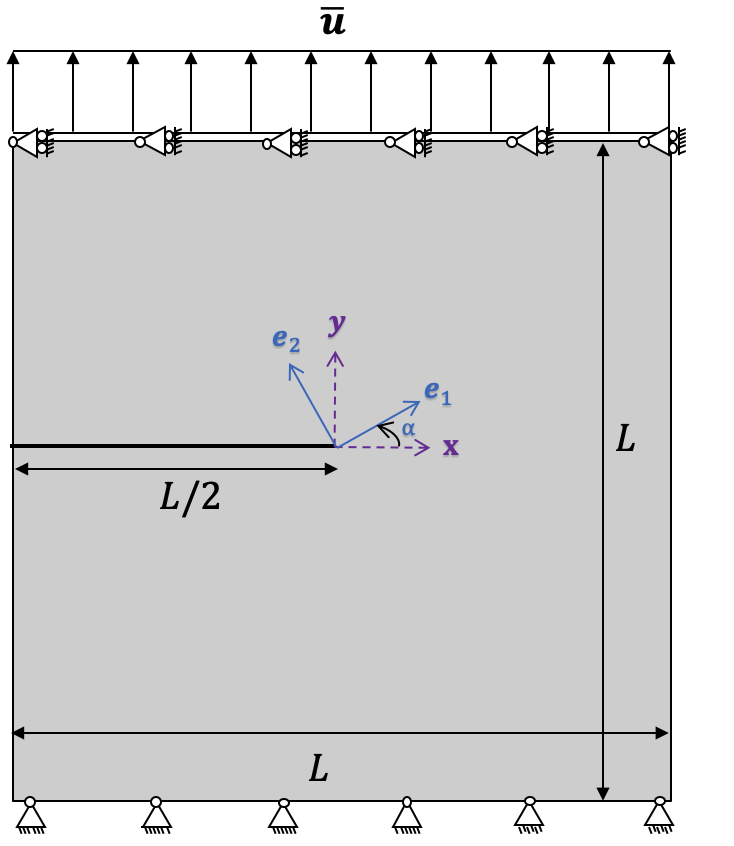
(a) tensile test

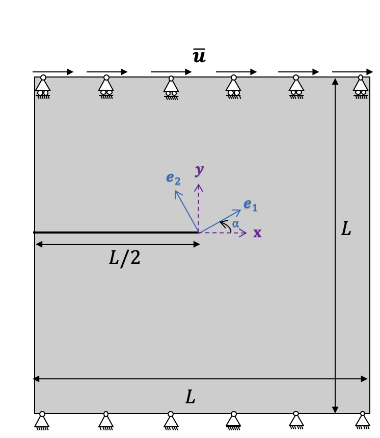
(b) shear test

Figure 1: Schematic of two cracked square plate under a displacement (a) tensile and (b) shear loading. An incremental displacement loading is applied on the top edges. The material principal axes ($\bm{e}_{1},\bm{e}_{2}$) have an angle of $\alpha$ with the original coordinate system ($\bm{x},\bm{y}$).

3.1 Tensile test

A pre-notched square plate loaded in tension was computed. For orthotropic volumetric-deviatoric and no-tension, the fracture response at the last step $\bar{\bm{u}}=2\times 10^{-5}$ m is shown in Figure 2 with four material orientation angles $\alpha=0$, $\pm\pi/4$, and $\pi/2$. It was observed that both models generate similar crack paths. When the material principal axes coincide with the symmetric axes ($\alpha=0$ or $\alpha=\pi/2$), the crack moves straightforward. In other cases ($\alpha=\pm\pi/4$), the crack slightly deviates from the straight path impacted by the orthotropic deformation.

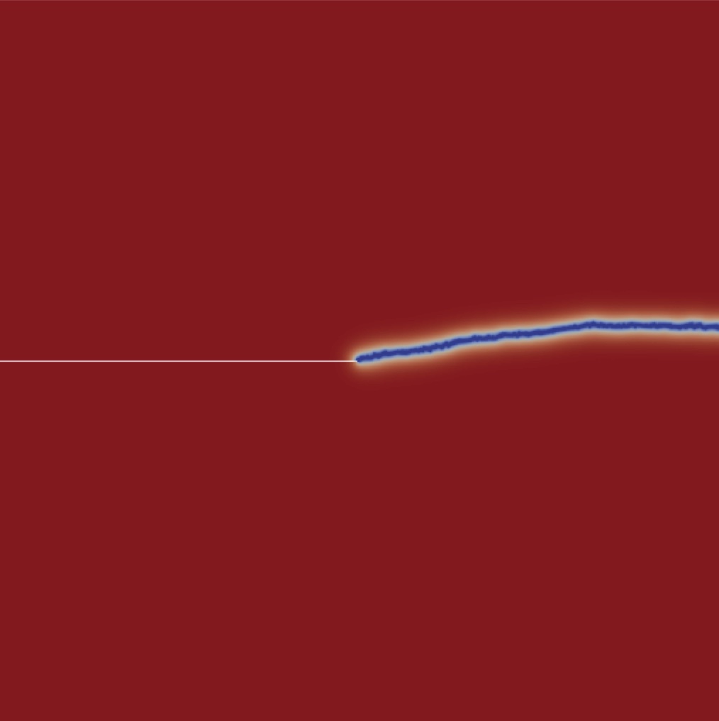
(a) volumetric-deviatoric, $\alpha=-\pi/4$

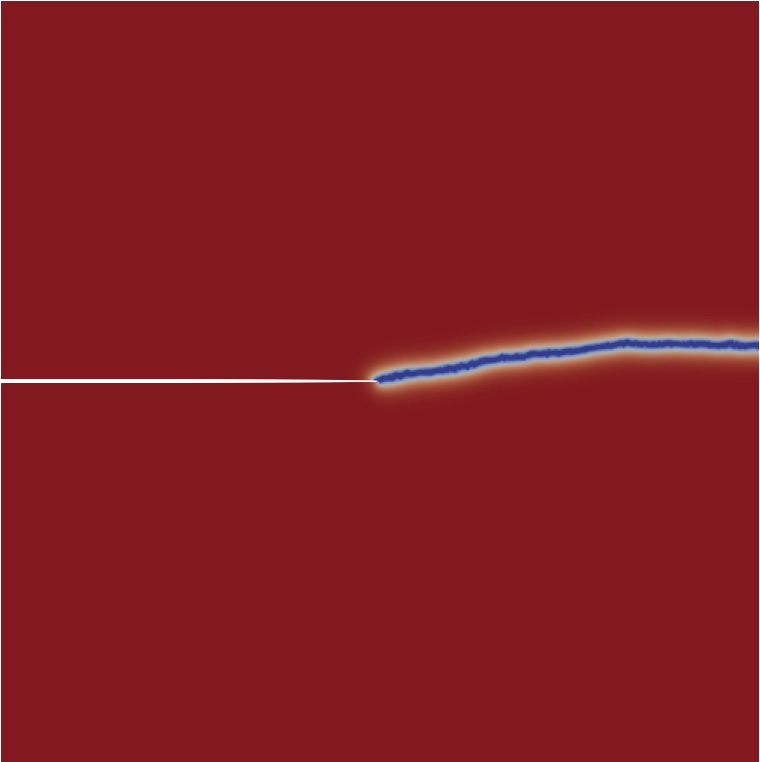
(b) no-tension, $\alpha=-\pi/4$

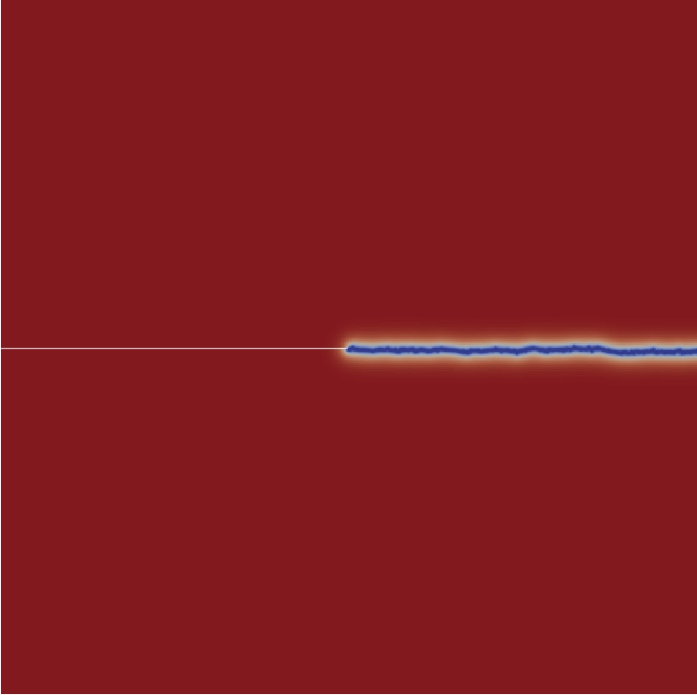
(c) volumetric-deviatoric, $\alpha=0$

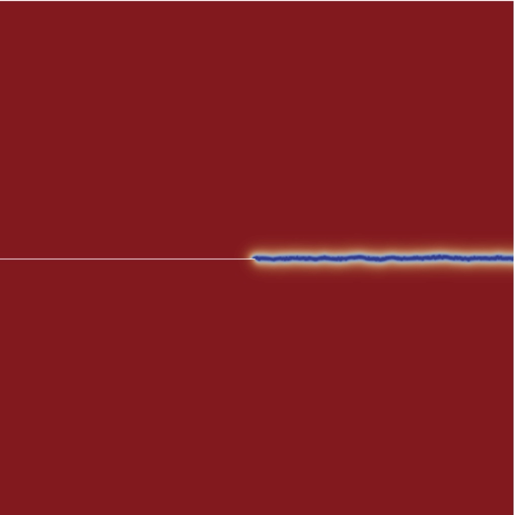
(d) no-tension, $\alpha=0$

(e) volumetric-deviatoric, $\alpha=\pi/4$

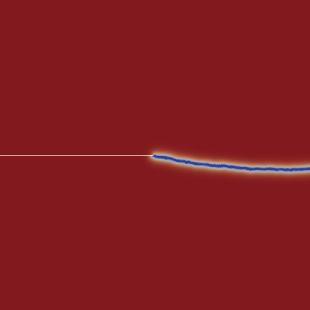
(f) no-tension, $\alpha=\pi/4$

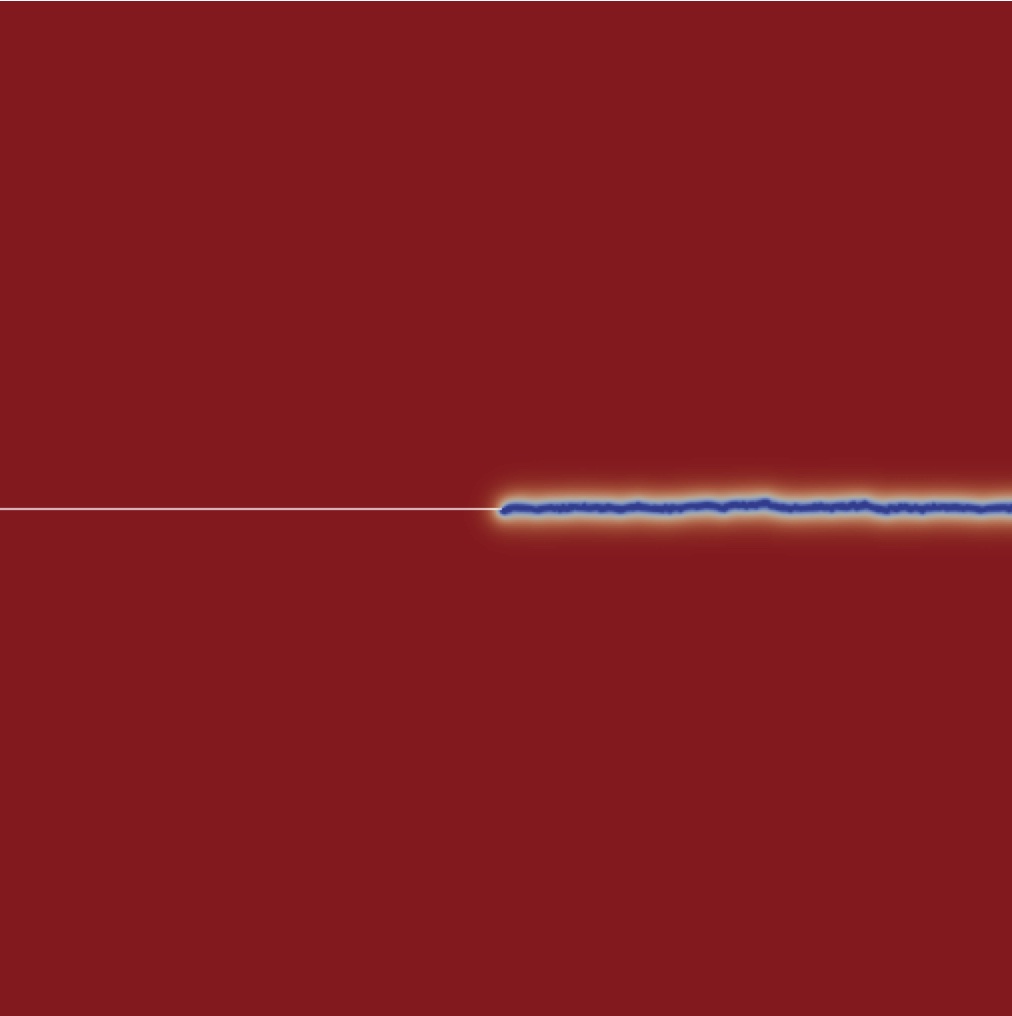
(g) volumetric-deviatoric, $\alpha=\pi/2$

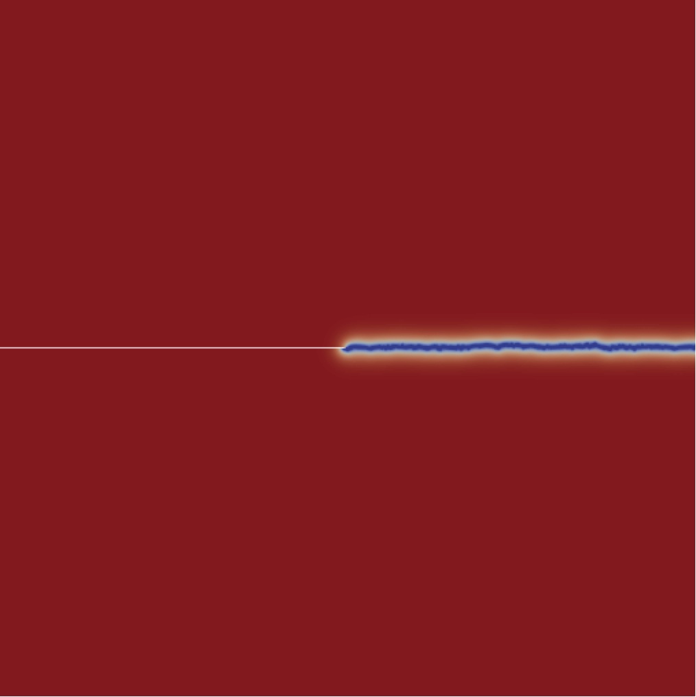
(h) no-tension, $\alpha=\pi/2$

Figure 2: Cracked square plate under tension. Phase field contours of orthotropic volumetric-deviatoric and no-tension at the last step with with $\bar{\bm{u}}=2\times 10^{-5}$ m. The same parameters were used for both models. Under tensile loading, we observe a similar crack response for both models. With four material orientation angles tested for both models, the crack propagates along the horizontal axis for $\alpha=0$ and $\alpha=\pi/2$. For $\alpha=\pm\pi/4$, the crack deviates slightly for both models as a consequence of orthotropy.

Figure 3 depicts the magnitude of the strain tensor at the stage of the crack initiation for orthotropic volumetric-deviatoric with four material orientation angles. With $\alpha=0$ or $\alpha=\pi/2$, the deformation is symmetry around the $x$-axis whereas a non-symmetric behavior can be seen for $\alpha=\pm\pi/4$ where the material principal axes deviate from the symmetric axes.

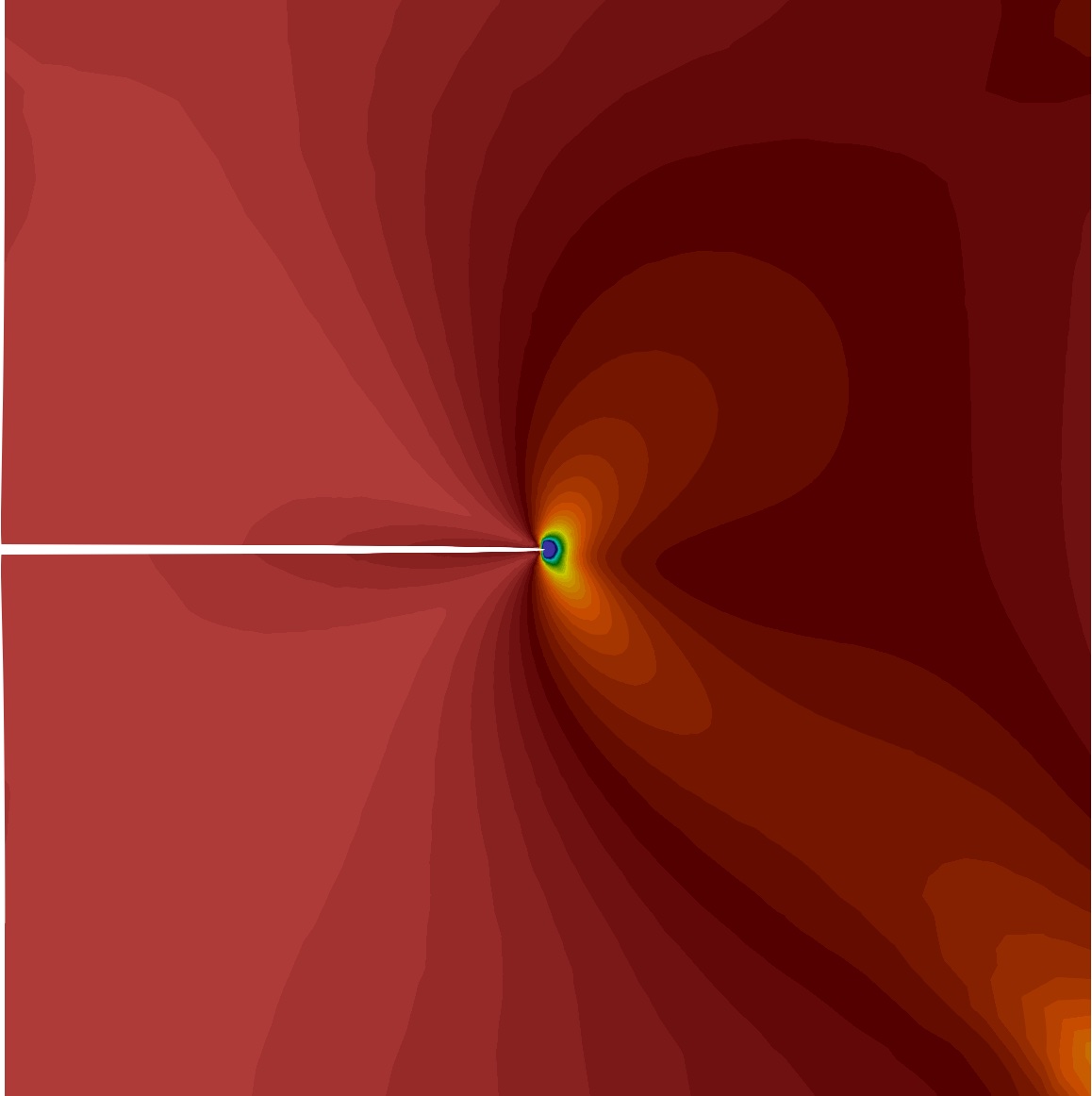
(a) $\alpha=-\pi/4$, $\bm{u}\approx 0.37\bar{\bm{u}}$

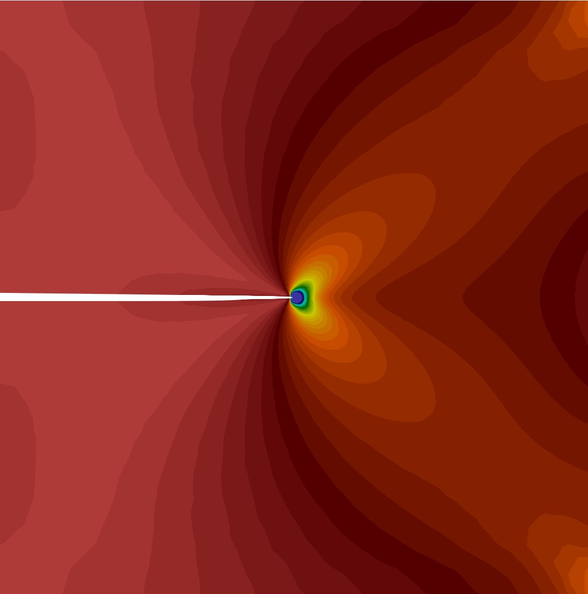
(b) $\alpha=0$, $\bm{u}\approx 0.47\bar{\bm{u}}$

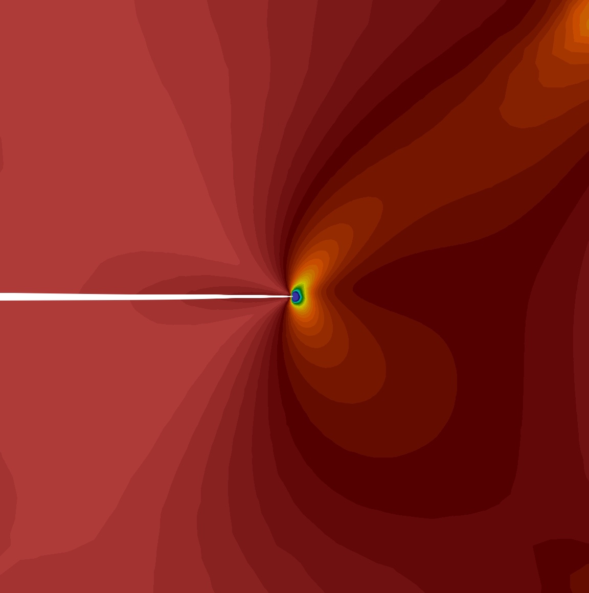
(c) $\alpha=\pi/4$, $\bm{u}\approx 0.36\bar{\bm{u}}$

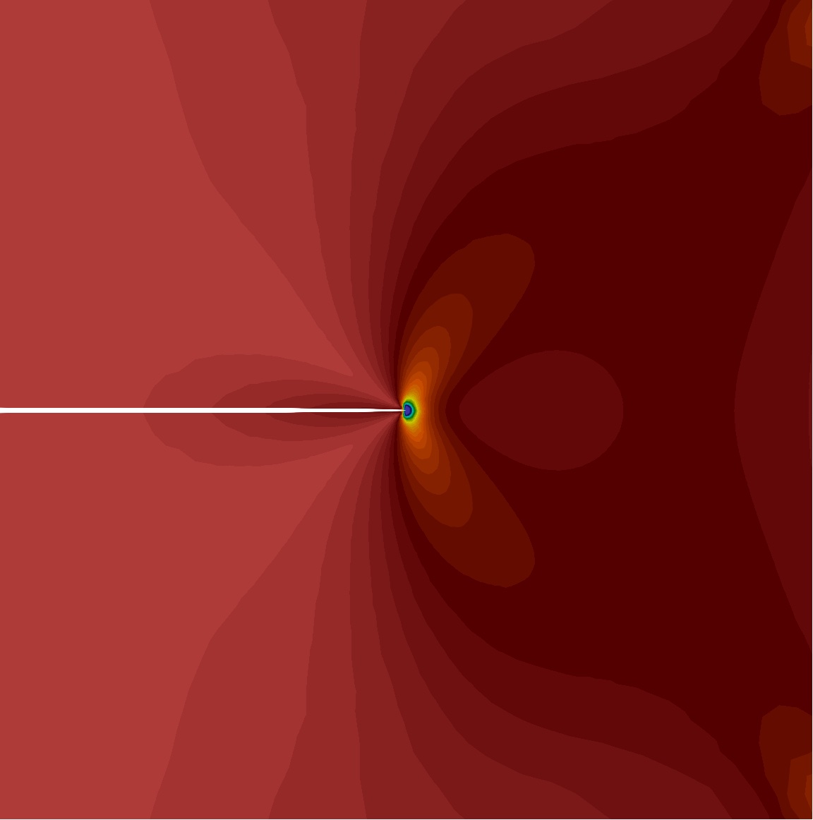
(d) $\alpha=\pi/2$, $\bm{u}\approx 0.30\bar{\bm{u}}$

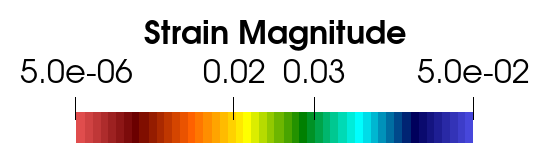
Figure 3: The magnitude of the strain tensor at the initiation of the crack for orthotropic volumetric-deviatoric with four material orientation angles. A symmetric behavior is observed for $\alpha=0$ and $\alpha=\pi/2$, while the magnitude is higher for $\alpha=0$ as the material has more stiffness along the horizontal axis. For $\alpha=\pm\pi/4$, asymmetry is observed where the magnitude is higher along the material principal axis with more stiffness.

Figure 4 shows the energy release rate computation using the $G_{\theta}$ method with our proposed modifications (see B) for both models with four material orientation angles. Crack propagation should follow the direction of the maximum energy dissipation [24, 17]. And it is observed that for all cases the maximum energy release rate directions are approximately along the crack paths. Moreover, both split models have the identical crack propagation paths under the tensile loading because the strain energies are all tensile and crack-driving. Also observed is the crack propagates at the same loading with $\alpha=\pm\pi/4$, but earlier with $\alpha=\pi/2$ than $\alpha=0$. This is because different stiffness in the principal loading direction require different displacement loads to build up the necessary strain energy for propagating the crack.

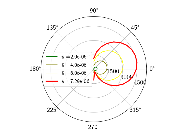
(a) volumetric-deviatoric, $\alpha=-\pi/4$

(b) no-tension, $\alpha=-\pi/4$

(c) volumetric-deviatoric, $\alpha=0$

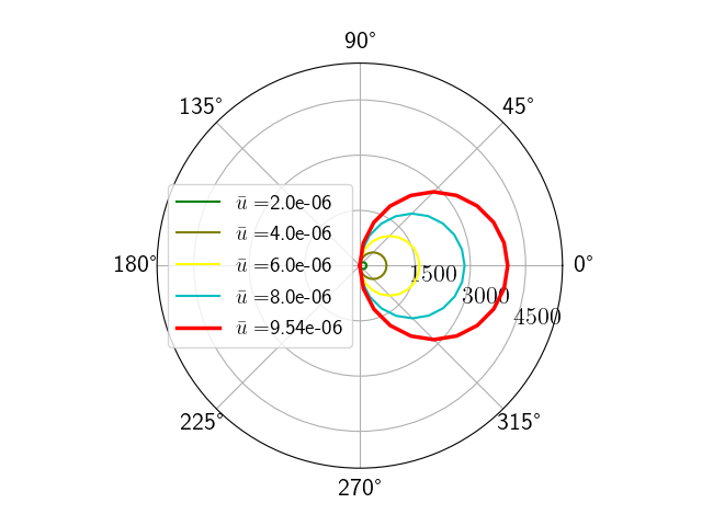
(d) no-tension, $\alpha=0$

(e) volumetric-deviatoric, $\alpha=\pi/4$

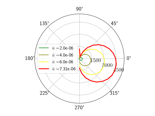
(f) no-tension, $\alpha=\pi/4$

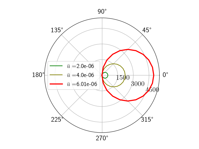
(g) volumetric-deviatoric, $\alpha=\pi/2$

(h) no-tension, $\alpha=\pi/2$

Figure 4: Under tensile loading for orthotropic volumetric-deviatoric and no-tension, we computed the energy release rate using the $G_{\theta}$ method with our proposed modifications. Several curves are plotted for a set of $\bar{\bm{u}}$ where the red ones correspond with the stage of crack initiation. The peak of each curve approximately aligns with the direction of crack propagation, see Figure 2. For $\alpha=0$ and $\alpha=\pi/2$, the peaks are along the horizontal line, whereas for $\alpha=\pm\pi/4$ the peaks deviate slightly from the $x$-axis. In both models, crack initiation occurs almost at the same loading for $\alpha=\pm\pi/4$ but in the opposite vertical directions, while the crack starts to propagate earlier for $\alpha=\pi/2$ compared to $\alpha=0$. This is expected due to the effect of orthotropy as the material is stiffer along the $y$-direction for $\alpha=\pi/2$.

3.2 Shear test

Figure 5 depicts the crack paths for orthotropic volumetric-deviatoric and no-tension under shear loading with four material orientation angles ($\alpha=-\pi/4$, 0, $\pi/4$, and $\pi/2$). In contrary to the tensile test, herein a significant difference in crack response is observed between the two models for all cases.

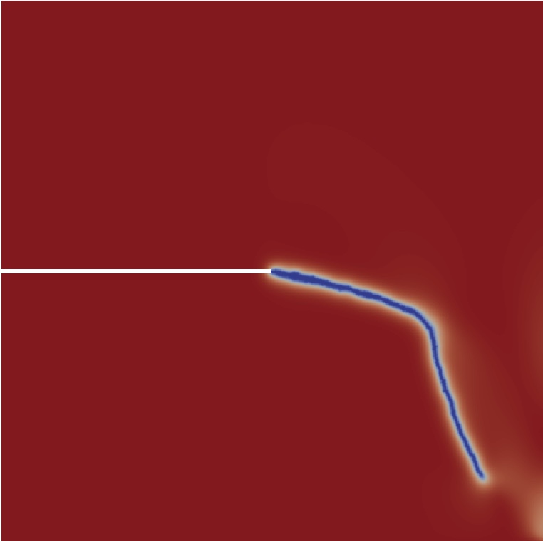
(a) volumetric-deviatoric, $\alpha=-\pi/4$

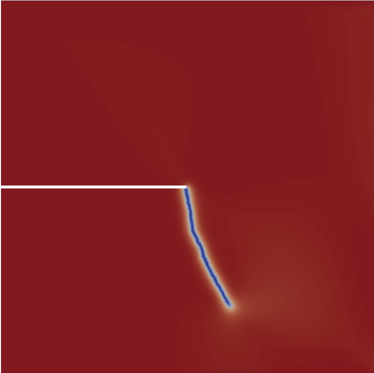
(b) no-tension, $\alpha=-\pi/4$

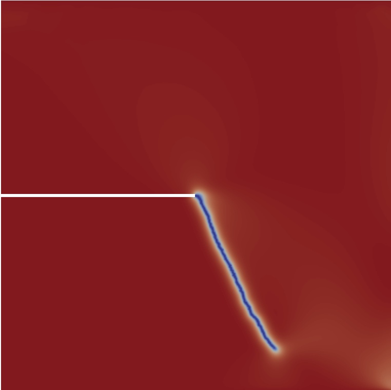
(c) volumetric-deviatoric, $\alpha=0$

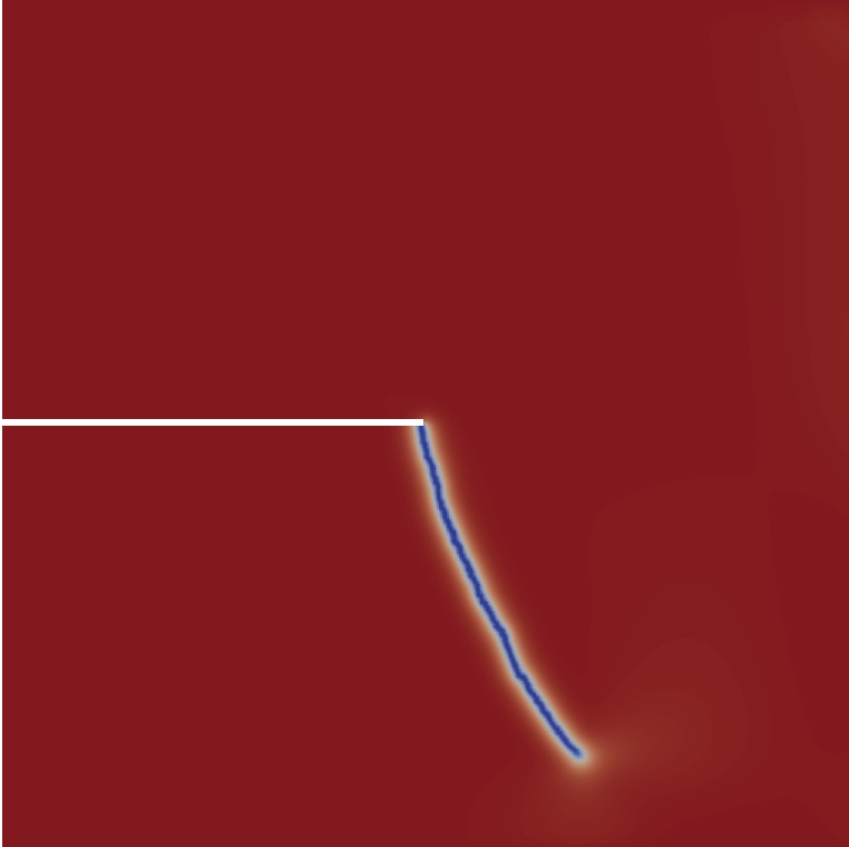
(d) no-tension, $\alpha=0$

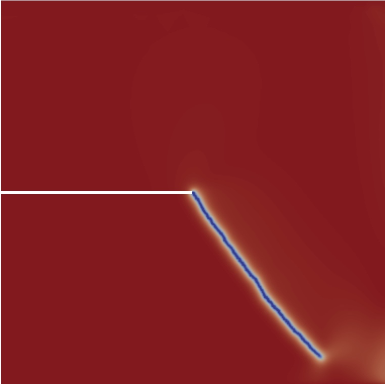
(e) volumetric-deviatoric, $\alpha=\pi/4$

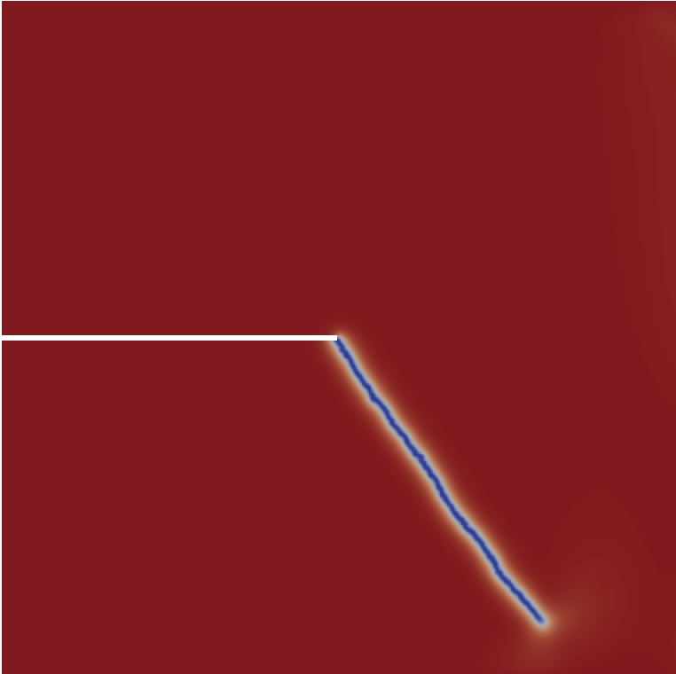
(f) no-tension, $\alpha=\pi/4$

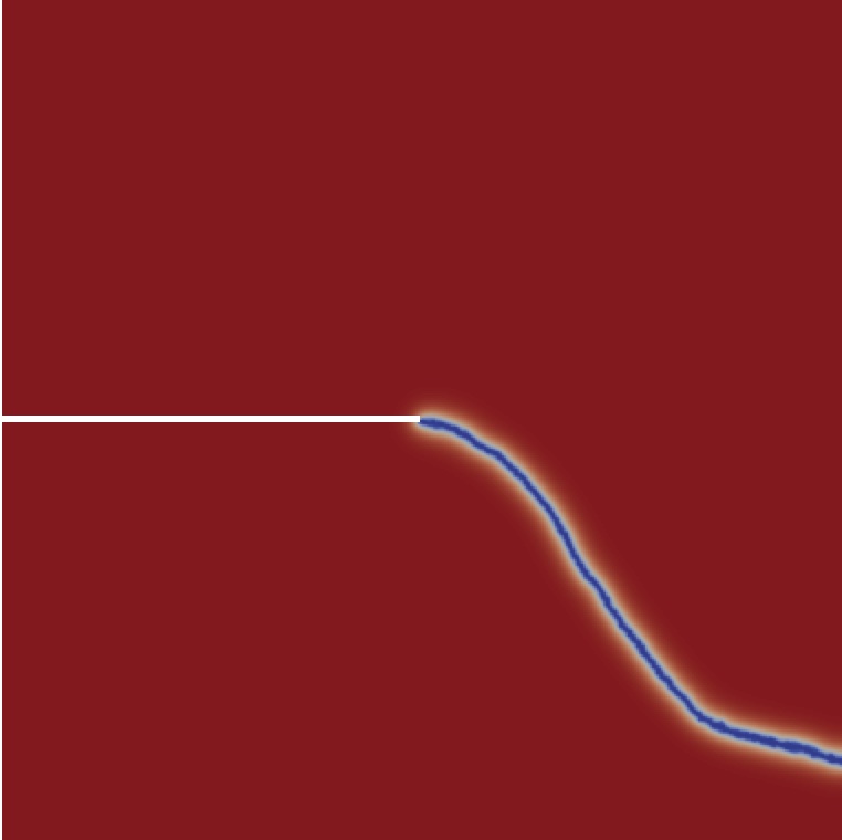
(g) volumetric-deviatoric, $\alpha=\pi/2$

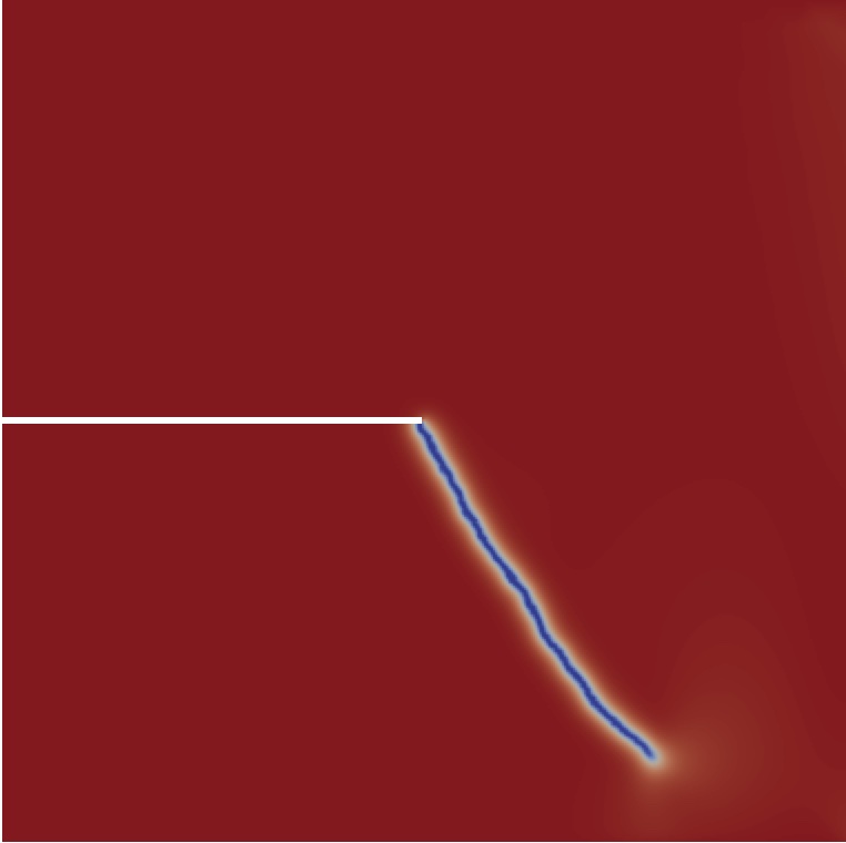
(h) no-tension, $\alpha=\pi/2$

Figure 5: Cracked square plate under shear. Phase field contours of orthotropic volumetric-deviatoric and no-tension at the last step with $\bar{\bm{u}}=2\times 10^{-5}$ m. The same parameters were used for both models. Here, we observe that the crack paths are different depending on the model and the material orientation. For $\alpha=0$ and $\alpha=\pi/4$, however, both models generate relatively similar crack responses. With $\alpha=\pi/4$ there exist straight cracks that grow towards the lower right corner, almost along the material principal axis with lower stiffness. Also, with $\alpha=\pi/4$ the crack propagates earlier than other cases because of the effect of orthotropy. In this case, the material has the least stiffness along the preferred direction of crack growth under shear loading.

Figure 6 plots the maximum energy release rate for both models with four material orientation angles. In most cases, the peaks are approximately along the crack propagation paths. Note, however, that the maximum energy release rate computed is higher than the critical value which may require further investigation.

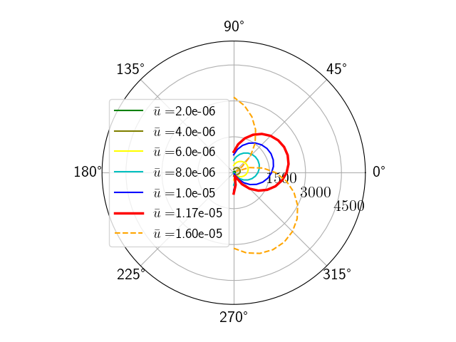
(a) volumetric-deviatoric, $\alpha=-\pi/4$

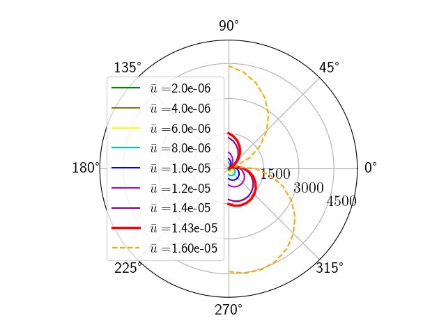
(b) no-tension, $\alpha=-\pi/4$

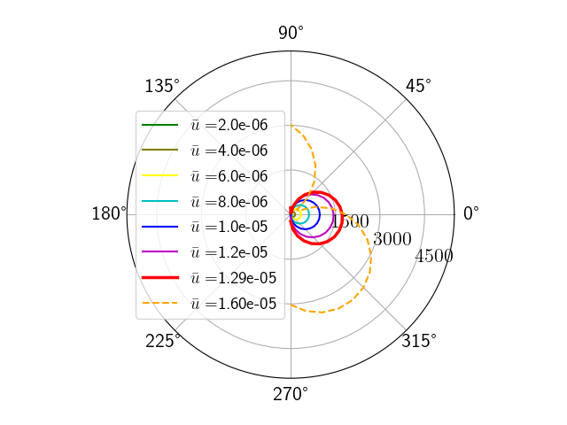
(c) volumetric-deviatoric, $\alpha=0$

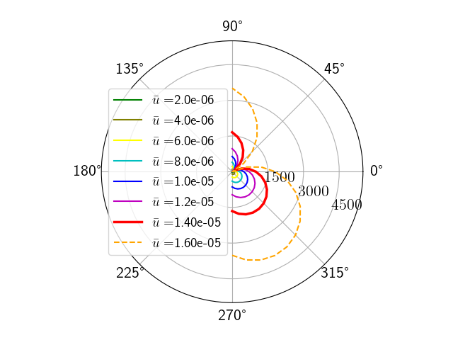
(d) no-tension, $\alpha=0$

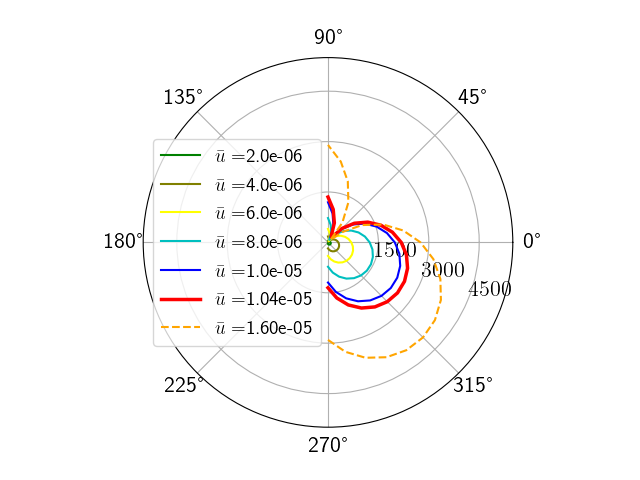
(e) volumetric-deviatoric, $\alpha=\pi/4$

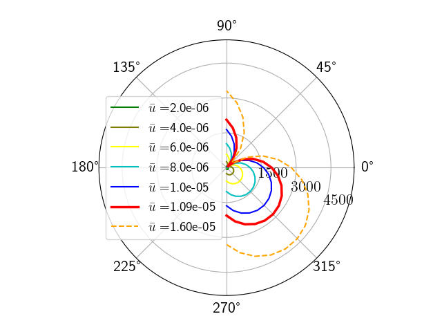
(f) no-tension, $\alpha=\pi/4$

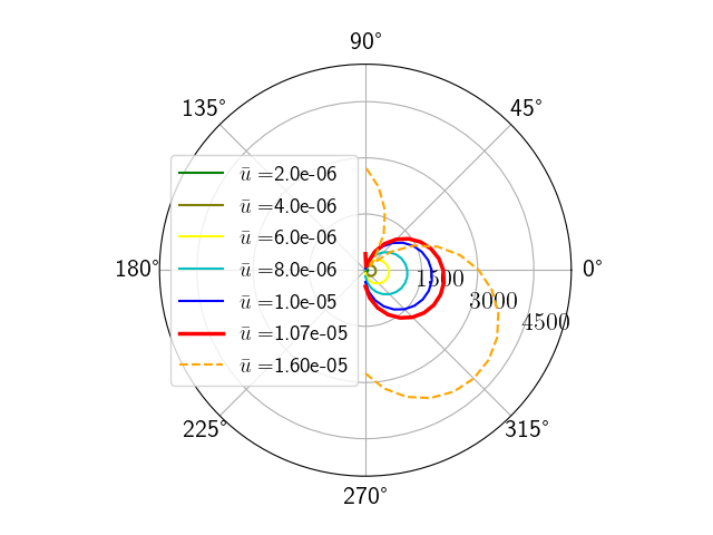
(g) volumetric-deviatoric, $\alpha=\pi/2$

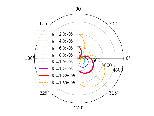
(h) no-tension, $\alpha=\pi/2$

Figure 6: Under shear loading for orthotropic volumetric-deviatoric and no-tension, we computed the energy release rate using the $G_{\theta}$ method with our proposed modifications. Several curves are plotted for a set of $\bar{\bm{u}}$ where the red curves correspond with the onset of crack propagation, and the orange ones refer to a fixed step thereafter for all samples, $\bar{\bm{u}}=1.6\times 10^{-5}$ m, where the crack is propagating towards the bottom-right corner. Like the tensile example, for most cases, the maximum energy release rate of each case approximately aligns with the direction of crack propagation (Figure 5). An exception is the case of $\alpha=-\pi/4$ for volumetric-deviatoric where the peak of the red curve deviates from the direction of crack propagation, whereas the orange curve fits better. Also observed is that crack initiation occurs earlier in no-tension for all cases.

Figures 7 show the load-deflection curves for the tensile examples (a–b) and the shear examples (c–d). All tensile examples result in a global stiffness loss, as the crack propagates through the sample. For the shear examples, only in one case (volumetric-deviatoric with $\alpha=\pi/2$), the crack reaches to the edge. In other cases, as soon as the crack propagates, the load drops. However this drop is not high and is recovered shortly in some cases.)

(a) volumetric-deviatoric, tension

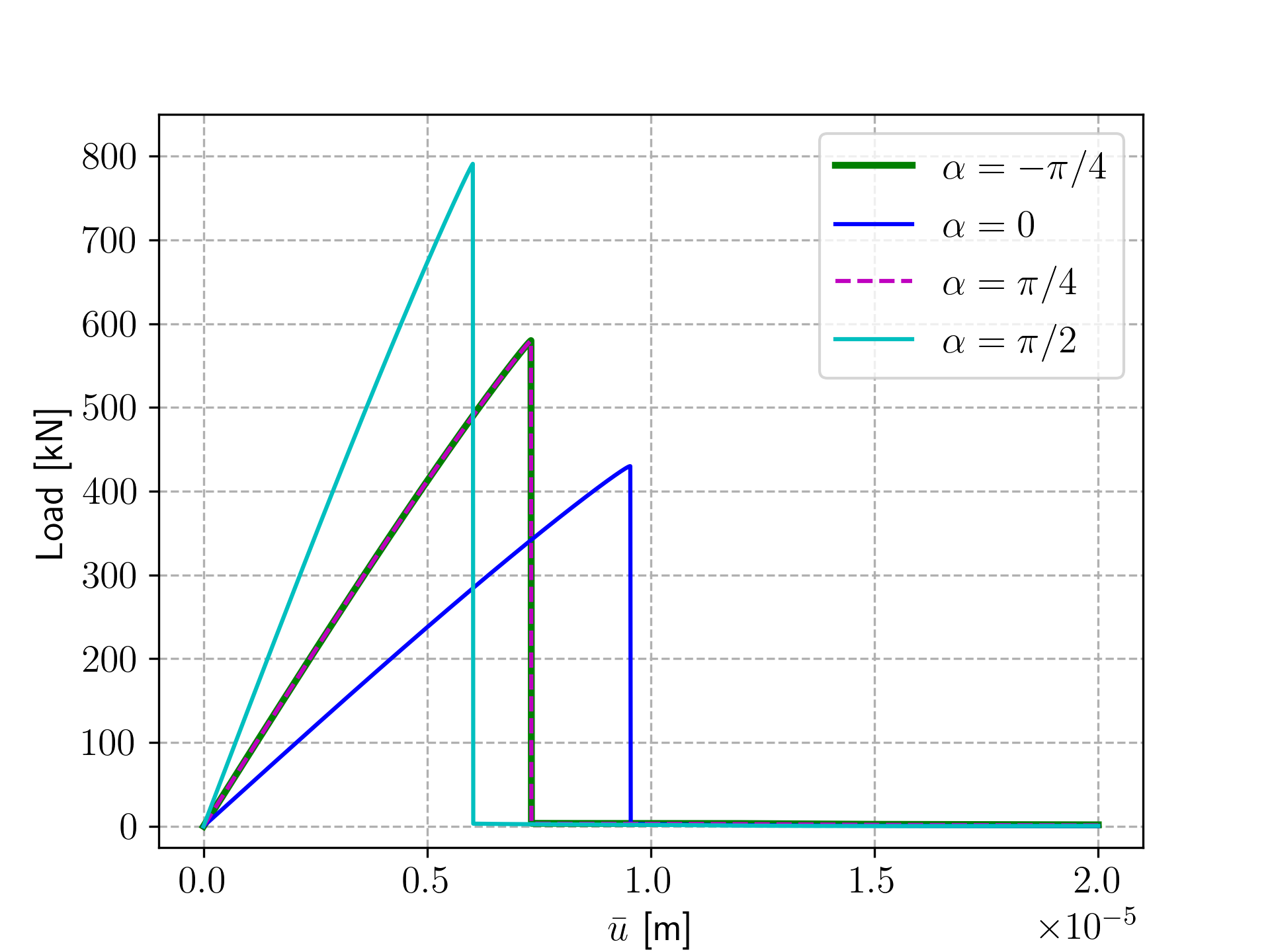
(b) no-tension, tension

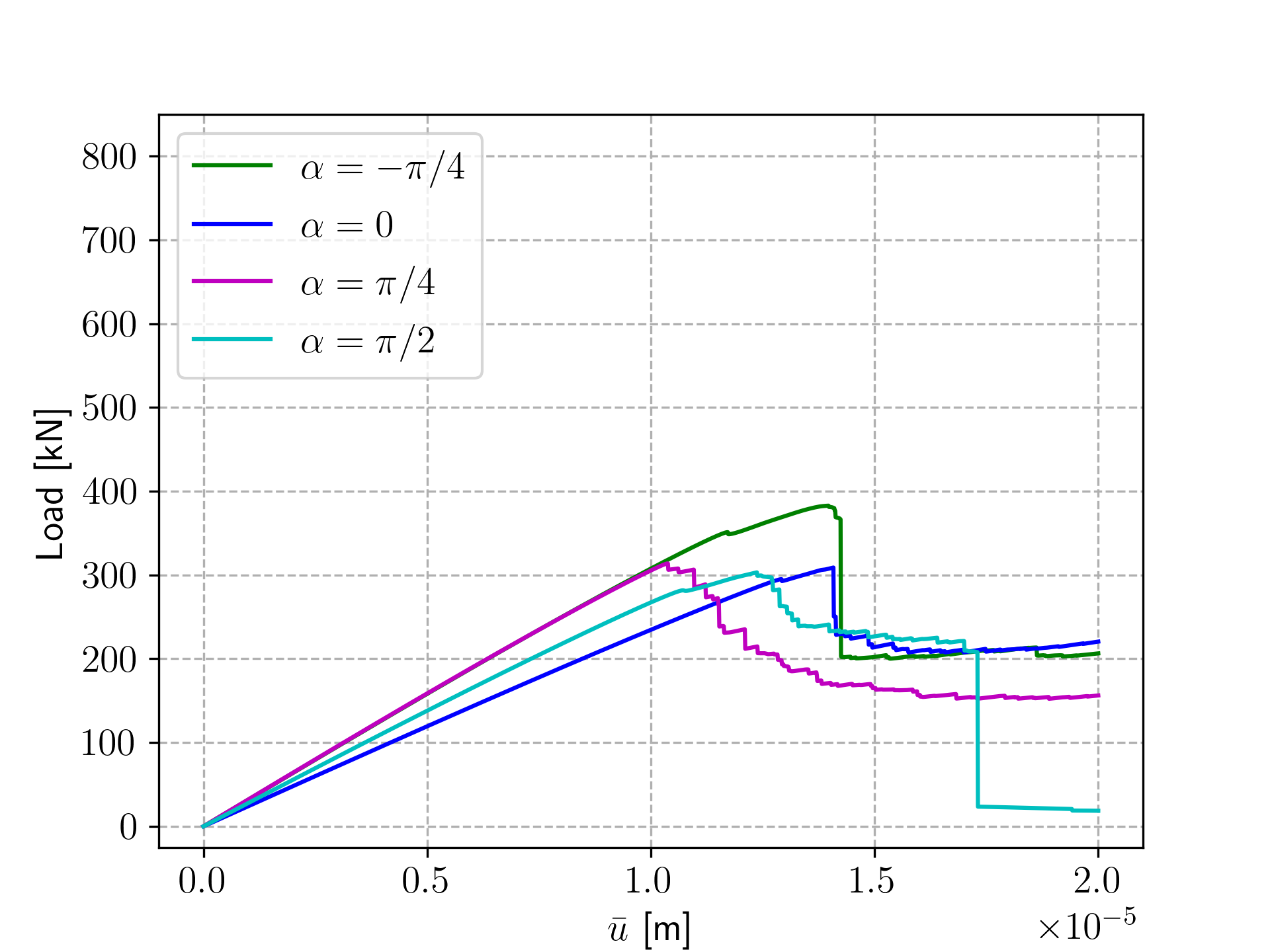
(c) volumetric-deviatoric, shear

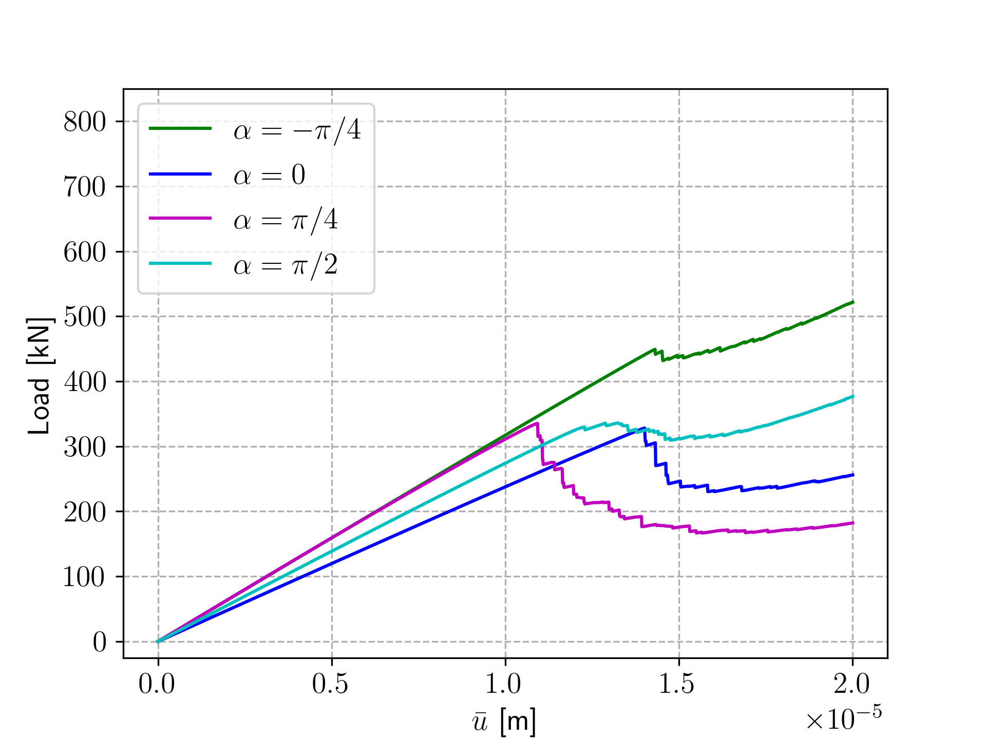
(d) no-tension, shear

Figure 7: Load deflection curves for both models under (a)–(b) tensile and (c)–(d) shear loading. For (a)–(b) a sudden loss of the stiffness indicates that the crack grows in an unstable manner. These load-displacment results show that the crack propagates at the same loading for $\alpha=\pm\pi/4$. For $\alpha=\pi/2$ the crack propagates earlier compared to $\alpha=0$ because the crack propagation direction aligns with the weaker material direction. For (c), the global stiffness is “lost” for the case of $\alpha=\pi/2$ in which the crack reaches to the edge. Also observed for all cases in (c)–(d) is that there is a drop in the load at the onset of crack propagation.

4 Conclusion

In this paper, we have proposed a method to account for orthotropy/anisotropy of materials when modeling tension-compression asymmetry in their crack response. Two decomposition models, volumetric-deviatoric and no-tension, were extended to capture arbitrary types of anisotropy in the constitutive behavior in a three-dimensional setting. A major characteristic of the formulation is that it keeps the variational formalism in partitioning the constitutive model, honoring the orthogonality condition.
The two models presented in this work were evaluated and compared numerically in a square plate with a pre-notched crack loaded in tension and shear. Under the tensile loading, the result indicates that both models have approximately similar responses. Testing different material orientation angles, the effect of orthotropy on the material response is clearly observed. To better interpret the results, we investigated the energy release rate using the $G_{\theta}$ method with our proposed modifications. And a significant difference in the resulting crack paths iss observed between the two models under shear loading. However, at this point it is difficult to judge which model provides a more reliable outcome.
The results presented herein highlight the importance of how to decompose the constitutive model of materials with anisotropic nature in the phase field approach to brittle fracture. As opposed to imposing anisotropic behaviors to the surface energy (fracture toughness), adapting the strain energy leads to ‘weak’ anisotropy [29]. However, some materials evidently exhibit anisotropic elastic deformation and this effect should not be ignored. Future studies should include ‘strong’ anisotropy by adding the directionality to the surface energy, and comparisons against experiments to determine whether both strong and weak anisotropy or how much of each is required.

Appendix A Projection tensors in two/three dimensions

For the two-dimensional case, the following closed-form expressions are adapted.

$$\mathbb{D}^{\text{t}}:=\frac{\partial\tilde{\bm{\varepsilon}}^{\text{t}}}{\partial\tilde{\bm{\varepsilon}}}=\begin{cases}\dfrac{a_{1}-a_{2}}{\tilde{\varepsilon}_{1}-\tilde{\varepsilon}_{2}}\Bigl{[}\mathds{1}_{S}-\bm{M}_{1}\otimes\bm{M}_{1}-\bm{M}_{2}\otimes\bm{M}_{2}\Bigr{]}\\ +H(\tilde{\varepsilon}_{1})\bm{M}_{1}\otimes\bm{M}_{1}+H(\tilde{\varepsilon}_{2})\bm{M}_{2}\otimes\bm{M}_{2},&\text{if}~{}\tilde{\varepsilon}_{1}\neq\tilde{\varepsilon}_{2}\\ H(\tilde{\varepsilon}_{1})\mathds{1}_{S},&\text{if}~{}\tilde{\varepsilon}_{1}=\tilde{\varepsilon}_{2}\end{cases}$$ (33a)

$$\mathbb{D}^{\text{c}}:=\frac{\partial\tilde{\bm{\varepsilon}}^{\text{c}}}{\partial\tilde{\bm{\varepsilon}}}=\begin{cases}\dfrac{b_{1}-b_{2}}{\tilde{\varepsilon}_{1}-\tilde{\varepsilon}_{2}}\Bigl{[}\mathds{1}_{S}-\bm{M}_{1}\otimes\bm{M}_{1}-\bm{M}_{2}\otimes\bm{M}_{2}\Bigr{]}\\ +H(-\tilde{\varepsilon}_{1})\bm{M}_{1}\otimes\bm{M}_{1}+H(-\tilde{\varepsilon}_{2})\bm{M}_{2}\otimes\bm{M}_{2},&\text{if}~{}\tilde{\varepsilon}_{1}\neq\tilde{\varepsilon}_{2}\\ H(-\tilde{\varepsilon}_{1})\mathds{1}_{S},&\text{if}~{}\tilde{\varepsilon}_{1}=\tilde{\varepsilon}_{2}\end{cases}$$ (33b)

where $\mathds{1}_{S}$ is the fourth-order tensor defined by:

$$(\mathds{1}_{S})_{ijkl}=\frac{1}{2}\bigl{(}\delta_{ik}\delta_{jl}+\delta_{il}\delta_{jk}\bigr{)}.$$

To derive the projection tensors ($\mathbb{D}^{\text{t}}$ and $\mathbb{D}^{\text{c}}$) with a three-dimensional basis in Kelvin-matrix notation, we proceed as follows. With (26), let the original coordinate system coincide with the material principal axes $\bm{n}_{i}$s. Thus, the only non-zero components of $\mathbb{D}^{t}$ and $\mathbb{D}^{c}$ on the basis $\bm{n}_{i}$ are given by:

$$D^{\text{t}}_{iiii}=H(\tilde{\varepsilon}_{i}),\quad D^{\text{c}}_{iiii}=H(-\tilde{\varepsilon}_{i}),$$ (34)

$$D^{\text{t}}_{ijij}=\begin{cases}\frac{1}{2}H(\tilde{\varepsilon}_{i})&\tilde{\varepsilon}_{i}=\tilde{\varepsilon}_{j},\quad i\neq j,\\ \frac{1}{2}\bigl{\{}H(\tilde{\varepsilon}_{j})\tilde{\varepsilon}_{j}-H(\tilde{\varepsilon}_{i})\tilde{\varepsilon}_{i}\bigr{\}}/(\tilde{\varepsilon}_{j}-\tilde{\varepsilon}_{i})&\tilde{\varepsilon}_{i}\neq\tilde{\varepsilon}_{j},\quad i\neq j,\end{cases}$$

$$D^{\text{c}}_{ijij}=\begin{cases}\frac{1}{2}H(-\tilde{\varepsilon}_{i})&\tilde{\varepsilon}_{i}=\tilde{\varepsilon}_{j},\quad i\neq j,\\ \frac{1}{2}\bigl{\{}H(-\tilde{\varepsilon}_{j})\tilde{\varepsilon}_{j}-H(-\tilde{\varepsilon}_{i})\tilde{\varepsilon}_{i}\bigr{\}}/(\tilde{\varepsilon}_{j}-\tilde{\varepsilon}_{i})&\tilde{\varepsilon}_{i}\neq\tilde{\varepsilon}_{j},\quad i\neq j.\end{cases}$$

The following projection tensors are then obtained for different cases (in Kelvin-matrix notation):

Case I

$\tilde{\bm{\varepsilon}}^{\text{t}}=(\tilde{\varepsilon}_{1},\tilde{\varepsilon}_{2},\tilde{\varepsilon}_{3})$ and $\tilde{\bm{\varepsilon}}^{\text{c}}=(0,0,0)$:

$$\undertilde{\bm{D}}^{\text{t}}=\begin{bmatrix}1&0&0&0&0&0\\ &1&0&0&0&0\\ &&1&0&0&0\\ &&&1&0&0\\ &&&&1&0\\ &&&&&1\end{bmatrix},\quad\undertilde{\bm{D}}^{\text{c}}=\begin{bmatrix}0&0&0&0&0&0\\ &0&0&0&0&0\\ &&0&0&0&0\\ &&&0&0&0\\ &&&&0&0\\ &&&&&0\end{bmatrix}.$$

Case II

$\tilde{\bm{\varepsilon}}^{\text{t}}=(\tilde{\varepsilon}_{1},\tilde{\varepsilon}_{2},0)$ and $\tilde{\bm{\varepsilon}}^{\text{c}}=(0,0,\tilde{\varepsilon}_{3})$:

$$\undertilde{\bm{D}}^{\text{t}}=\begin{bmatrix}1&0&0&0&0&0\\ &1&0&0&0&0\\ &&0&0&0&0\\ &&&1&0&0\\ &&&&\tilde{\varepsilon}_{1}/(\tilde{\varepsilon}_{1}-\tilde{\varepsilon}_{3})&0\\ &&&&&\tilde{\varepsilon}_{2}/(\tilde{\varepsilon}_{2}-\tilde{\varepsilon}_{3})\end{bmatrix},\quad\undertilde{\bm{D}}^{\text{c}}=\begin{bmatrix}0&0&0&0&0&0\\ &0&0&0&0&0\\ &&1&0&0&0\\ &&&0&0&0\\ &&&&-\tilde{\varepsilon}_{3}/(\tilde{\varepsilon}_{1}-\tilde{\varepsilon}_{3})&0\\ &&&&&-\tilde{\varepsilon}_{3}/(\tilde{\varepsilon}_{2}-\tilde{\varepsilon}_{3})\end{bmatrix}.$$

Case III

$\tilde{\bm{\varepsilon}}^{\text{t}}=(\tilde{\varepsilon}_{1},0,0)$ and $\tilde{\bm{\varepsilon}}^{\text{c}}=(0,\tilde{\varepsilon}_{2},\tilde{\varepsilon}_{3})$:

$$\undertilde{\bm{D}}^{\text{t}}=\begin{bmatrix}1&0&0&0&0&0\\ &0&0&0&0&0\\ &&0&0&0&0\\ &&&\tilde{\varepsilon}_{1}/(\tilde{\varepsilon}_{1}-\tilde{\varepsilon}_{2})&0&0\\ &&&&\tilde{\varepsilon}_{1}/(\tilde{\varepsilon}_{1}-\tilde{\varepsilon}_{3})&0\\ &&&&&0\end{bmatrix},\quad\undertilde{\bm{D}}^{\text{c}}=\begin{bmatrix}0&0&0&0&0&0\\ &1&0&0&0&0\\ &&1&0&0&0\\ &&&-\tilde{\varepsilon}_{2}/(\tilde{\varepsilon}_{1}-\tilde{\varepsilon}_{2})&0&0\\ &&&&-\tilde{\varepsilon}_{3}/(\tilde{\varepsilon}_{1}-\tilde{\varepsilon}_{3})&0\\ &&&&&1\end{bmatrix}.$$

Case IV

$\tilde{\bm{\varepsilon}}^{\text{t}}=(0,0,0)$ and $\tilde{\bm{\varepsilon}}^{\text{c}}=(\tilde{\varepsilon}_{1},\tilde{\varepsilon}_{2},\tilde{\varepsilon}_{3})$:

$$\undertilde{\bm{D}}^{\text{t}}=\begin{bmatrix}0&0&0&0&0&0\\ &0&0&0&0&0\\ &&0&0&0&0\\ &&&0&0&0\\ &&&&0&0\\ &&&&&0\end{bmatrix},\quad\undertilde{\bm{D}}^{\text{c}}=\begin{bmatrix}1&0&0&0&0&0\\ &1&0&0&0&0\\ &&1&0&0&0\\ &&&1&0&0\\ &&&&1&0\\ &&&&&1\end{bmatrix}.$$

The projection tensors in Kelvin-matrix notation, $\undertilde{\bm{D}}^{\text{t}}$ and $\undertilde{\bm{D}}^{\text{c}}$ can also be derived for an arbitrary orthonormal basis with a transformation as follows

$$\undertilde{\bm{D}}^{\prime\text{t}}=\bm{P}\undertilde{\bm{D}}^{\text{t}}\bm{P}^{T},\quad\undertilde{\bm{D}}^{\prime\text{c}}=\bm{P}\undertilde{\bm{D}}^{\text{c}}\bm{P}^{T},$$ (35)

where $\undertilde{\bm{D}}^{\prime\text{t}}$ and $\undertilde{\bm{D}}^{\prime\text{c}}$ are represented in the new basis.

Appendix B Energy release rate computation: $G_{\theta}$ method

The $G_{\theta}$ method is based on the estimation of the second derivatives of the energy potential with respect to crack length using the technique of virtual domain perturbation $\bm{\theta}$ [19]. Numerically it uses an integral over a surface, which is more accurate than the contour integral used in the J-integral [47]. Denoting the tangential vector to the crack tip as $\bm{t}$, we can use the virtual domain perturbation:

$$\bm{\theta}=f(r)\bm{t},$$ (36)

where

$$f(r)=\begin{cases}1&\;\text{for }r<r_{i}\\ \dfrac{r-r_{o}}{r_{i}-r_{o}}&\;\text{for }r_{i}<r<r_{o}\\ 0&\;\text{for }r_{o}<r\end{cases}$$ (37)

and $r$ is the distance from the crack tip, and $r_{i}$ and $r_{o}$ are set as $r_{i}=4\ell$ and $r_{o}=2.5r_{i}$ in this study (Figure 8). With $\bm{\theta}$, the energy release rate is computed as

$$G_{\theta}=\int_{\Omega}\bm{\sigma}:(\nabla\mathbf{u}\nabla\bm{\theta})-\frac{1}{2}(\bm{\sigma}:\nabla\mathbf{u})\nabla\cdot\bm{\theta}\,\mathrm{d}x.$$ (38)

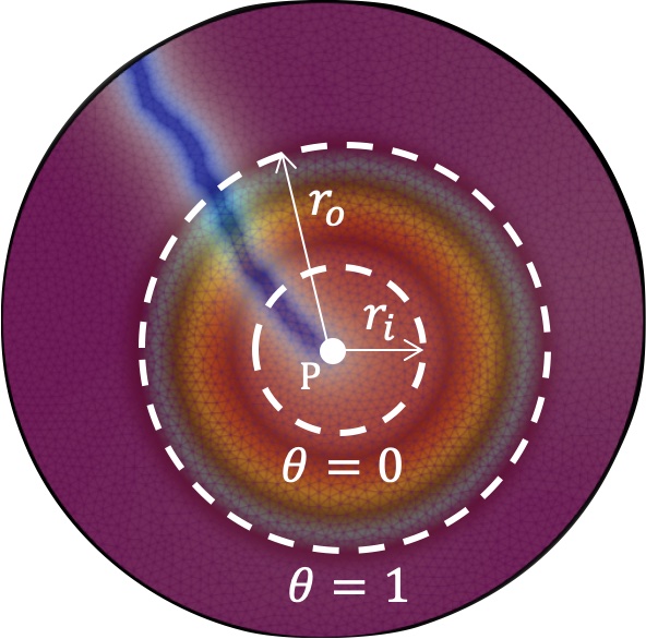
Figure 8: Phase field and $\theta$ profile for volumetric-deviatoric, $\alpha=0$ at $t_{f}$ under shear loading. We use virtual perturbation of $\theta$ to compute energy release rate using $G_{\theta}$. The $\theta$ value is 1 inside of $B_{r_{i}}(P)$, 0 outside, and a linear interpolation in between. We set $r_{i}=4\ell$ and $r_{o}=2.5r_{i}$.

However, the energy release rates computed by (38) do not seem to predict the fracture propagation direction properly (Figure 9 (a)). For this reason, considering the tension-compression asymmetry, we decompose $\mathbf{u}^{t}$ as

$$\nabla\mathbf{u}=\nabla\mathbf{u}^{t}+\nabla\mathbf{u}^{c}.$$

Then we define the tensile part of the energy release rate as

$$G_{\theta}^{t}=\int_{\Omega}\bm{\sigma}^{t}:(\nabla\mathbf{u}^{t}\nabla\bm{\theta})-\frac{1}{2}(\bm{\sigma}^{t}:\nabla\mathbf{u}^{t})\nabla\cdot\bm{\theta}\,\mathrm{d}x.$$ (39)

While $\bm{\sigma}^{t}$ can be straightforwardly obtained from $\mathbb{C}\bm{\varepsilon}^{t}$, the tensile part of the displacement $\mathbf{u}^{t}$ is not defined in any of the strain energy split models. Here, we assume that the compressive part of the displacement $\nabla\mathbf{u}^{c}$ is symmetric i.e., $(\nabla\mathbf{u}^{c})=(\nabla\mathbf{u}^{c})^{\mathrm{T}}$. Then we have

$$\bm{\varepsilon}^{c}=\nabla\mathbf{u}^{c}.$$

and

$$\nabla\mathbf{u}^{t}=\nabla\mathbf{u}-\bm{\varepsilon}^{c}.$$ (40)

Figure 9 illustrates the effects of the modified computation using the tensile part of the displacement, $G_{\theta}^{t}$ . Without the modifications (Figure 9 (a)), the maximum energy release rates point to an incorrect propagation direction (straight fracture propagation) prior to the propagation. With our proposed modifications (Figure 9 (b)), the direction predicted by the energy release rates coincide with the actual propagation direction.

(a) $G_{\theta}$

(b) $G_{\theta}^{t}$

Figure 9: Comparison (a) energy release rate $G_{\theta}$ with (b) tensile part of energy release rate for no-tension, $\alpha=0$ under shear loading. In terms of directionality, tensile part of energy release rate accurately depicts the fracture propagation direction before and after fracture starts to propagate.

References

- Alessi et al., [2018] Alessi, R., Marigo, J.-J., Maurini, C., and Vidoli, S. (2018). Coupling damage and plasticity for a phase-field regularisation of brittle, cohesive and ductile fracture: One–dimensional examples. International Journal of Mechanical Sciences, 149:559–576.
- Alessi et al., [2014] Alessi, R., Marigo, J.-J., and Vidoli, S. (2014). Gradient damage models coupled with plasticity and nucleation of cohesive cracks. Archive for Rational Mechanics and Analysis, 214(2):575–615.
- Amadei, [1996] Amadei, B. (1996). Importance of anisotropy when estimating and measuring in situ stresses in rock. International Journal of Rock Mechanics and Mining Sciences & Geomechanics Abstracts, 33(3):293–325.
- Ambati et al., [2015] Ambati, M., Gerasimov, T., and De Lorenzis, L. (2015). Phase-field modeling of ductile fracture. Computational Mechanics, 55(5):1017–1040.
- Amor et al., [2009] Amor, H., Marigo, J.-J., and Maurini, C. (2009). Regularized formulation of the variational brittle fracture with unilateral contact: Numerical experiments. Journal of the Mechanics and Physics of Solids, 57(8):1209–1229.
- Baldelli et al., [2014] Baldelli, A. L., Babadjian, J.-F., Bourdin, B., Henao, D., and Maurini, C. (2014). A variational model for fracture and debonding of thin films under in-plane loadings. Journal of the Mechanics and Physics of Solids, 70:320–348.
- Bilgen and Weinberg, [2021] Bilgen, C. and Weinberg, K. (2021). A phase-field approach to pneumatic fracture with anisotropic crack resistance. International Journal of Fracture, 232(2):135–151.
- Bilke et al., [2019] Bilke, L., Flemisch, B., Kalbacher, T., Kolditz, O., Helmig, R., and Nagel, T. (2019). Development of open-source porous media simulators: Principles and experiences. Transport in Porous Media, 130(1):337–361.
- Bleyer and Alessi, [2018] Bleyer, J. and Alessi, R. (2018). Phase-field modeling of anisotropic brittle fracture including several damage mechanisms. Computer Methods in Applied Mechanics and Engineering, 336:213–236.
- Borden et al., [2012] Borden, M., Verhoosel, C., Scott, M., Hughes, T., and Landis, C. (2012). A phase-field description of dynamic brittle fracture. Computer Methods in Applied Mechanics and Engineering, 217-220:77–95.
- Bourdin et al., [2012] Bourdin, B., Chukwudozie, C., and Yoshioka, K. (2012). A variational approach to the numerical simulation of hydraulic fracturing. In SPE ATCE 2012.
- Bourdin et al., [2000] Bourdin, B., Francfort, G., and Marigo, J.-J. (2000). Numerical experiments in revisited brittle fracture. J. Mech. and Phys. of Solids, 48(4):797–826.
- Bourdin and Francfort, [2019] Bourdin, B. and Francfort, G. A. (2019). Past and present of variational fracture. SIAM News, 52(9).
- Bourdin et al., [2011] Bourdin, B., Larsen, C., and Richardson, C. (2011). A time-discrete model for dynamic fracture based on crack regularization. International Journal of Fracture, 168(2):133–143.
- Bryant and Sun, [2018] Bryant, E. C. and Sun, W. (2018). A mixed-mode phase field fracture model in anisotropic rocks with consistent kinematics. Computer Methods in Applied Mechanics and Engineering, 342:561–584.
- Carcione, [1995] Carcione, J. M. (1995). Constitutive model and wave equations for linear, viscoelastic, anisotropic media. Geophysics, 60(2):537–548.
- Chambolle et al., [2009] Chambolle, A., Francfort, G. A., and Marigo, J.-J. (2009). When and how do cracks propagate? Journal of the Mechanics and Physics of Solids, 57(9):1614–1622.
- De Lorenzis and Maurini, [2021] De Lorenzis, L. and Maurini, C. (2021). Nucleation under multi-axial loading in variational phase-field models of brittle fracture. International Journal of Fracture, pages 1–21.
- Dubois et al., [1998] Dubois, F., Chazal, C., and Petit, C. (1998). A finite element analysis of creep-crack growth in viscoelastic media. Mechanics Time-Dependent Materials, 2(3):269–286.
- Fei and Choo, [2021] Fei, F. and Choo, J. (2021). Double-phase-field formulation for mixed-mode fracture in rocks. Computer Methods in Applied Mechanics and Engineering, 376:113655.
- Francfort and Marigo, [1998] Francfort, G. A. and Marigo, J.-J. (1998). Revisiting brittle fracture as an energy minimization problem. Journal of the Mechanics and Physics of Solids, 46(8):1319–1342.
- Freddi and Royer-Carfagni, [2010] Freddi, F. and Royer-Carfagni, G. (2010). Regularized variational theories of fracture: A unified approach. Journal of the Mechanics and Physics of Solids, 58(8):1154–1174.
- Gerasimov and De Lorenzis, [2022] Gerasimov, T. and De Lorenzis, L. (2022). Second-order phase-field formulations for anisotropic brittle fracture. Computer Methods in Applied Mechanics and Engineering, 389:114403.
- Hakim and Karma, [2009] Hakim, V. and Karma, A. (2009). Laws of crack motion and phase-field models of fracture. Journal of the Mechanics and Physics of Solids, 57(2):342–368.
- He and Shao, [2019] He, Q.-C. and Shao, Q. (2019). Closed-Form Coordinate-Free Decompositions of the Two-Dimensional Strain and Stress for Modeling Tension–Compression Dissymmetry. Journal of Applied Mechanics, 86(3).
- Heider and Markert, [2017] Heider, Y. and Markert, B. (2017). A phase-field modeling approach of hydraulic fracture in saturated porous media. Mechanics Research Communications, 80:38–46.
- Heng et al., [2015] Heng, S., Guo, Y., Yang, C., Daemen, J. J., and Li, Z. (2015). Experimental and theoretical study of the anisotropic properties of shale. International Journal of Rock Mechanics and Mining Sciences, 74:58–68.
- Kuhn et al., [2016] Kuhn, C., Noll, T., and Müller, R. (2016). On phase field modeling of ductile fracture. GAMM Mitteilungen, 39(1):35–54.
- Li and Maurini, [2019] Li, B. and Maurini, C. (2019). Crack kinking in a variational phase-field model of brittle fracture with strongly anisotropic surface energy. Journal of the Mechanics and Physics of Solids, 125:502–522.
- Li et al., [2015] Li, B., Peco, C., Millán, D., Arias, I., and Arroyo, M. (2015). Phase-field modeling and simulation of fracture in brittle materials with strongly anisotropic surface energy. International Journal for Numerical Methods in Engineering, 102(3-4):711–727.
- Li et al., [2021] Li, C., Yang, D., Xie, H., Ren, L., and Wang, J. (2021). Research on the anisotropic fracture behavior and the corresponding fracture surface roughness of shale. Engineering Fracture Mechanics, 255:107963.
- Li et al., [2016] Li, T., Marigo, J.-J., Guilbaud, D., and Potapov, S. (2016). Gradient damage modeling of brittle fracture in an explicit dynamics context. International Journal for Numerical Methods in Engineering, 108(11):1381–1405.
- Luo et al., [2022] Luo, Z., Chen, L., Wang, N., and Li, B. (2022). A phase-field fracture model for brittle anisotropic materials. Computational Mechanics, pages 1–13.
- Marigo et al., [2016] Marigo, J.-J., Maurini, C., and Pham, K. (2016). An overview of the modelling of fracture by gradient damage models. Meccanica, 51(12):3107–3128.
- Martínez-Pañeda et al., [2018] Martínez-Pañeda, E., Golahmar, A., and Niordson, C. F. (2018). A phase field formulation for hydrogen assisted cracking. Computer Methods in Applied Mechanics and Engineering, 342:742–761.
- Miehe et al., [2016] Miehe, C., Aldakheel, F., and Raina, A. (2016). Phase field modeling of ductile fracture at finite strains: A variational gradient-extended plasticity-damage theory. International Journal of Plasticity, 84:1–32.
- [37] Miehe, C., Hofacker, M., and Welschinger, F. (2010a). A phase field model for rate-independent crack propagation: Robust algorithmic implementation based on operator splits. Computer Methods in Applied Mechanics and Engineering, 199(45):2765–2778.
- [38] Miehe, C., Welschinger, F., and Hofacker, M. (2010b). Thermodynamically consistent phase-field models of fracture: variational principles and multi-field FE implementations. International Journal for Numerical Methods in Engineering, 83(February):1273–1311.
- Moerman et al., [2016] Moerman, K. M., Simms, C. K., and Nagel, T. (2016). Control of tension–compression asymmetry in Ogden hyperelasticity with application to soft tissue modelling. Journal of the Mechanical Behavior of Biomedical Materials, 56:218–228.
- Nguyen et al., [2020] Nguyen, T.-T., Yvonnet, J., Waldmann, D., and He, Q.-C. (2020). Implementation of a new strain split to model unilateral contact within the phase field method. International Journal for Numerical Methods in Engineering, 121(21):4717–4733.
- Nguyen and Wu, [2018] Nguyen, V. P. and Wu, J.-Y. (2018). Modeling dynamic fracture of solids with a phase-field regularized cohesive zone model. Computer Methods in Applied Mechanics and Engineering, 340:1000–1022.
- Nixon et al., [2010] Nixon, M. E., Cazacu, O., and Lebensohn, R. A. (2010). Anisotropic response of high-purity -titanium: Experimental characterization and constitutive modeling. International Journal of Plasticity, 26(4):516–532.
- Noii et al., [2020] Noii, N., Aldakheel, F., Wick, T., and Wriggers, P. (2020). An adaptive global–local approach for phase-field modeling of anisotropic brittle fracture. Computer Methods in Applied Mechanics and Engineering, 361:112744.
- Parisio and Laloui, [2018] Parisio, F. and Laloui, L. (2018). On the formulation of anisotropic–polyaxial failure criteria: a comparative study. Rock Mechanics and Rock Engineering, 51(2):479–489.
- Pham et al., [2011] Pham, K., Amor, H., Marigo, J.-J., and Maurini, C. (2011). Gradient damage models and their use to approximate brittle fracture. International Journal of Damage Mechanics, 20(4):618–652.
- Rezaei et al., [2022] Rezaei, S., Harandi, A., Brepols, T., and Reese, S. (2022). An anisotropic cohesive fracture model: advantages and limitations of length-scale insensitive phase-field damage models. Engineering Fracture Mechanics, page 108177.
- Rice and Rosengren, [1968] Rice, J. R. and Rosengren, G. (1968). Plane strain deformation near a crack tip in a power-law hardening material. Journal of the Mechanics and Physics of Solids, 16(1):1–12.
- Schuler et al., [2020] Schuler, L., Ilgen, A. G., and Newell, P. (2020). Chemo-mechanical phase-field modeling of dissolution-assisted fracture. Computer Methods in Applied Mechanics and Engineering, 362:112838.
- Steinke and Kaliske, [2019] Steinke, C. and Kaliske, M. (2019). A phase-field crack model based on directional stress decomposition. Computational Mechanics, 63(5):1019–1046.
- Teichtmeister et al., [2017] Teichtmeister, S., Kienle, D., Aldakheel, F., and Keip, M.-A. (2017). Phase field modeling of fracture in anisotropic brittle solids. International Journal of Non-Linear Mechanics, 97:1–21.
- Ulloa et al., [2022] Ulloa, J., Wambacq, J., Alessi, R., Samaniego, E., Degrande, G., and François, S. (2022). A micromechanics-based variational phase-field model for fracture in geomaterials with brittle-tensile and compressive-ductile behavior. Journal of the Mechanics and Physics of Solids, 159:104684.
- van Dijk et al., [2020] van Dijk, N., Espadas-Escalante, J., and Isaksson, P. (2020). Strain energy density decompositions in phase-field fracture theories for orthotropy and anisotropy. International Journal of Solids and Structures, 196-197:140–153.
- Wang et al., [2019] Wang, Y., Tan, W., Liu, D., Hou, Z., and Li, C. (2019). On anisotropic fracture evolution and energy mechanism during marble failure under uniaxial deformation. Rock Mechanics and Rock Engineering, 52(10):3567–3583.
- Wheeler et al., [2014] Wheeler, M., Wick, T., and Wollner, W. (2014). An augmented-Lagrangian method for the phase-field approach for pressurized fractures. Computer Methods in Applied Mechanics and Engineering, 271:69–85.
- Wilson and Landis, [2016] Wilson, Z. and Landis, C. (2016). Phase-field modeling of hydraulic fracture. Journal of the Mechanics and Physics of Solids, 96:264–290.
- Wu and Nguyen, [2018] Wu, J.-Y. and Nguyen, V. P. (2018). A length scale insensitive phase-field damage model for brittle fracture. Journal of the Mechanics and Physics of Solids, 119:20–42.
- Yin and Kaliske, [2020] Yin, B. and Kaliske, M. (2020). A ductile phase-field model based on degrading the fracture toughness: Theory and implementation at small strain. Computer Methods in Applied Mechanics and Engineering, 366:113068.
- Yoshioka et al., [2021] Yoshioka, K., Mollaali, M., and Kolditz, O. (2021). Variational phase-field fracture modeling with interfaces. Computer Methods in Applied Mechanics and Engineering, 384:113951.
- Yoshioka et al., [2019] Yoshioka, K., Parisio, F., Naumov, D., Lu, R., Kolditz, O., and Nagel, T. (2019). Comparative verification of discrete and smeared numerical approaches for the simulation of hydraulic fracturing. GEM - International Journal on Geomathematics, 10(1).
- You et al., [2021] You, T., Waisman, H., and Zhu, Q.-Z. (2021). Brittle-ductile failure transition in geomaterials modeled by a modified phase-field method with a varying damage-driving energy coefficient. International Journal of Plasticity, 136:102836.
- Zhou et al., [2018] Zhou, S., Zhuang, X., and Rabczuk, T. (2018). A phase-field modeling approach of fracture propagation in poroelastic media. Engineering Geology, 240:189–203.