Quantum particle in a spherical well confined by a cone

Abstract

We consider the quantum problem of a particle in either a spherical box or a finite spherical well confined by a circular cone with an apex angle $2\theta_{0}$ emanating from the center of the sphere, with $0<\theta_{0}<\pi$. This non-central potential can be solved by an extension of techniques used in spherically-symmetric problems. The angular parts of the eigenstates depend on azimuthal angle $\varphi$ and polar angle $\theta$ as $P_{\lambda}^{m}(\cos\theta){\rm e}^{im\varphi}$ where $P_{\lambda}^{m}$ is the associated Legendre function of integer order $m$ and (usually noninteger) degree $\lambda$. There is an infinite discrete set of values $\lambda=\lambda_{i}^{m}$ ($i=0,1,3,\dots$) that depend on $m$ and $\theta_{0}$. Each $\lambda_{i}^{m}$ has an infinite sequence of eigenenergies $E_{n}(\lambda_{i}^{m})$, with corresponding radial parts of eigenfunctions. In a spherical box the discrete energy spectrum is determined by the zeros of the spherical Bessel functions. For several $\theta_{0}$ we demonstrate the validity of Weyl’s continuous estimate ${\cal N}_{W}$ for the exact number of states $\cal N$ up to energy $E$, and evaluate the fluctuations of $\cal N$ around ${\cal N}_{W}$. We examine the behavior of bound states in a well of finite depth $U_{0}$, and find the critical value $U_{c}(\theta_{0})$ when all bound states disappear. The radial part of the zero energy eigenstate outside the well is $1/r^{\lambda+1}$, which is not square-integrable for $\lambda\leq 1/2$. ($0<\lambda\leq 1/2$ can appear for $\theta_{0}>\theta_{c}\approx 0.726\pi$ and has no parallel in spherically-symmetric potentials.) Bound states have spatial extent $\xi$ which diverges as a (possibly $\lambda$-dependent) power law as $U_{0}$ approaches the value where the eigenenergy of that state vanishes.

1 Introduction

Closed form solutions of the non-relativistic Schrödinger equation for a single particle are useful for intuitive understanding of quantum mechanics [1]. Unfortunately, exact solutions are not very common. Even in one dimension (1D) the list of “simple,” analytically solvable, potentials is rather short: it includes the trivial cases of “particle in a box” or finite-depth square well potential, harmonic oscillator, and a list of moderate length of additional potentials [2, 3, 4], or potentials that can be reduced to such simple potentials by appropriate transformations (see, e.g., [5] and references therein). In higher dimensions, “exactly solvable” problems are usually reduced to a sequence of 1D problems, such as separation of the $d$-dimensional “particle in a rectangular box” problem into $d$ 1D problems in Cartesian coordinates, or similar separation of a $d$-dimensional harmonic oscillator into 1D oscillators. (In exceptional cases not amenable to variable separation, alternative methods based on supersymmetry or shape invariance exist [6, 7].) For central potentials, such as Coulomb interaction, or “spherical box” or finite spherical well, the simplification is achieved by separating the radial equation from the angular part, while the angular part in $d\geq 3$ can also be separated into several differential equations corresponding to various angles such as the polar angle $\theta$ and the azimuthal angle $\varphi$ in three dimensions (3D) [5].

In this work we consider a particle either confined in a 3D spherical box or placed in a finite depth spherical well. In both cases the allowed space is also confined by a rigid cone of apex angle $2\theta_{0}$ with the apex located at the center of the sphere. The resulting potential is not spherically-symmetric, i.e. non-central, but it can be solved using a slight extension of central potential methods which would be used in the absence of the confining cone. The angle $\theta_{0}$ is a dimensionless parameter that can qualitatively modify the solutions of Schrödinger equation and introduce some features the are absent in the central potential cases.

Besides the pedagogical value of this particular quantum problem as well as applicability to small quantum systems with similar geometry, it is also related to several classical problems: (a) When $i\partial/\partial t$ in the Schrödinger equation is replaced by $\partial/\partial t$, it resembles a diffusion equation, with quantum potential $V({\bf r})$ proportional to particle production or absorption rate at position ${\bf r}$, while a combination of other constants is proportional to a diffusion constant; it is one of the simpler forms of the Fokker-Planck equation [8]. (b) For long ideal polymers the partition function $Z$ satisfies an equation resembling the Schrödinger equation [9] with time replaced by imaginary $iN$, where $N$ is the number of monomers, and the quantum potential $V$ replaced by the potential of the polymer problem divided by $k_{B}T$ (cf., Ref. [10]). (Sequence of the instantaneous monomer positions ${\bf r}(i)$, where $i$ is the monomer number, can also be viewed as a time sequence ${\bf r}(t)$ of a diffusing particle, thus mapping the polymer problem onto a diffusion problem.) In the polymer problem the usual dependence of the quantum state with energy $E$ on time $\sim{\rm e}^{iEt/\hbar}$ is replaced by the polymer length dependence $\sim{\rm e}^{-EN}$, and therefore it is dominated by the ground state. The presence or absence of bound states in the quantum problem corresponds to the presence or absence of adsorption in the polymer problem [10, 11].

The 3D problems that are not spherically symmetric are usually not exactly solvable. However, a particular class of non-central potentials that has the form [12, 13]

$$V(r,\theta,\varphi)=U(r)+\frac{f(\theta)}{r^{2}}+\frac{g(\varphi)}{r^{2}\sin^{2}\theta}$$ (1)

can be separated in a form resembling central potentials. In classical physics, such a Hamiltonian has three constants of motion [14], while in Schrödinger equation the parts dependent of $\theta$ and $\varphi$ have the form that is naturally present when the equation is written in spherical coordinates, and the resulting equation separates into an azimuthal ($\varphi$-dependent) part that has a possibly non-integer eigenvalue $m$, which appears in the eigenvalue equation for the polar ($\theta$-dependent) part with possibly non-integer eigenvalue $\lambda$. Of course, separation of the Schrödinger equation into three one dimensional equations does not by itself make it exactly solvable, but for a certain collection of potentials it is possible to express the solutions via known functions and even provide algebraic expressions for the eigenvalues [12, 13]. For central potentials the angular parts have integer eigenvalues $m$ and $\lambda=\ell$, and the angular functions are spherical harmonics $Y_{\ell m}(\theta,\varphi)$.

In this work we consider a potential without azimuthal dependence ($g(\varphi)=0$), thus leaving that part of eigenfunction in the standard form (${\rm e}^{im\varphi}$ with integer $m$) familiar from central potentials [1]. The polar part of the potential represents the confinement of a particle inside an infinite circular cone

$$f(\theta)=\begin{cases}0,&\theta<\theta_{0},\\ \infty,&\text{otherwise}.\end{cases}$$ (2)

Such a potential does not introduce additional energy scales, but forces the polar part of the eigenfunction to vanish for $\theta=\theta_{0}$. For the particular case of $\theta_{0}=\pi/2$ it represents a repulsive plane. By itself, the infinite conical surface is length scale-free and represents an interesting case for many physical problems described by a Laplacian in the presence of a conical boundary, such as as problems of heat conduction or diffusion near cones [15], or polymers attached to conical probes [16, 17, 18, 19], or Casimir forces experienced by conical conductors [20], or diffraction of electromagnetic [21, 22, 23, 24] and acoustic [25] waves by conical surfaces.

If the apex of the confining cone is placed in the center of a spherical box or a finite spherical well of radius $a$, then the angle $\theta_{0}$ controls the length scale $a\theta_{0}$ and therefore strongly influences the eigenstates of the system. However, a change in $\theta_{0}$ does not modify the angular part of the Schrödinger equation, but only imposes boundary conditions on that part of the wavefunction.

In Sec. 2 we demonstrate the variable separation in Schrödinger equation for a particle in a spherical box, and show the $\theta_{0}$-dependence of the angular constants and the energy eigenvalues. We also study the structure of eigenvalue bunches that are created, and the behavior of the eigenvalues for $\theta_{0}$ near $\pi$ or 0. In Sec. 3 we verify the validity of a continuous function that estimates the number of states up to a certain energy $E$, and study the deviations of the exact results from the continuous estimates. Similar techniques are used in Sec. 4 to study a particle in a finite spherical well. Special attention is paid to the presence or absence of bound states. In Sec. 5 we examine the properties of zero-energy eigenstates that appear for special values of the well depth and show that for large $\theta_{0}$ some eigenstates are not normalizable. We show that, when the decreasing well depth approaches the condition where eigenenergy of a particular state vanishes, the spatial extent of the eigenfunction diverges with an exponent that may depend on $\theta_{0}$. In Sec. 6 we compare some our results with analogous properties of spherically-symmetric potentials, and also discuss the application of our results to polymer adsorption.

2 Infinite potential well

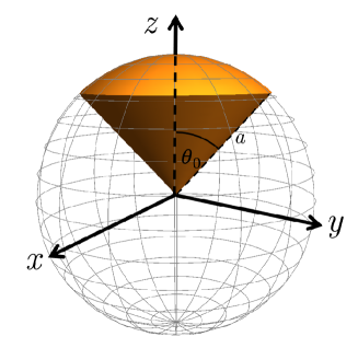
Figure 1: Spherical box (infinite potential well) of radius $a$ bounded by a cone with apex angle $2\theta_{0}$ (orange volume), with the symmetry axis along the Cartesian $z$ axis.

As a simplest example of a central potential confined by a conical surface, we consider a quantum particle of mass $m$ in a 3D spherical box (infinite potential well) of radius $a$ bounded by a cone with apex angle $2\theta_{0}$, such that the complete potential can be written as

$$V\left(\text{{r}}\right)=\begin{cases}0,&r<a,\,\theta<\theta_{0},\\ \infty,&\text{otherwise},\end{cases}$$ (3)

where the radius $r$ and polar angle $\theta$ are the spherical coordinates. An example of such confining space is represented in Fig. 1. It is convenient to work with dimensionless variables, where distances are measured in the units of sphere radius $a$, while the energies are measured in the units of $\hbar^{2}/2ma^{2}$. The time-independent Schrödinger equation [1] in these dimensionless variables is

$$\left(-\nabla^{2}+V\right)\psi=E\psi,$$ (4)

where $E$ is the energy eigenvalue and $\psi$ is the eigenfunction. In the absence of a confining cone, a spherical box is a textbook example [1] of a confined particle. In the presence of a cone, we follow a similar path of solving the equation by separation of variables, which in spherical coordinates leads to

$$-\frac{1}{r^{2}}\left[\frac{\partial}{\partial r}\left(r^{2}\frac{\partial}{\partial r}\right)+\frac{1}{\sin\theta}\frac{\partial}{\partial\theta}\left(\sin\theta\frac{\partial}{\partial\theta}\right)+\frac{1}{\sin^{2}\theta}\frac{\partial^{2}}{\partial\varphi^{2}}\right]\psi\\ +V\psi=E\psi.$$ (5)

As in the case of a central potential the solution can be separated into a product of radial, polar and azimuthal functions $\psi(r,\theta,\varphi)=R(r)\Theta(\theta)\Phi(\varphi)$. Since, the potential in Eq. (2) is independent of $\varphi$, the azimuthal part of the eigenstate satisfies the same equation as in the case of central potentials

$$-\frac{d^{2}\Phi}{d\varphi^{2}}=m^{2}\Phi,$$ (6)

which is satisfied by the functions $\Phi_{m}(\varphi)={\rm e}^{im\varphi}$ with $m=0,\pm 1,\pm 2,\dots$. These are eigenstates of the $z$ component of the angular momentum since the potential is invariant under rotations around $z$ axis.

The equation for the polar function $\Theta(\theta)$ coincides with the usual equation used for a central potential, since the restricting cone in Eq. (2) only influences the boundary conditions ($\Theta(\theta_{0})=0$) but does not otherwise affect the differential equation. The function $\Theta(\theta)$ obeys the general Legendre equation, in the variable $x=\cos\theta$, which in terms of polar angle $\theta$ has the form

$$\left[\frac{1}{\sin\theta}\frac{d}{d\theta}\left(\sin\theta\frac{d}{d\theta}\right)-\frac{m^{2}}{\sin^{2}\theta}\right]\Theta=-\lambda\left(\lambda+1\right)\Theta,$$ (7)

where the eigenvalue $-\lambda(\lambda+1)$ is expressed in terms of the constant $\lambda$ called the degree of the equation. In the absence of a confining cone, the degree of this equation has integer values $\lambda=\ell$, with $\ell\geq|m|$, and the eigenfunctions are given by the associated Legendre polynomials of $\cos\theta$ of order $m$ and degree $\ell$, $\Theta(\theta)=P^{m}_{\ell}(\cos\theta)$, and as a result the entire angular part of the eigenfunction is a spherical harmonic $Y_{\ell}^{m}\propto P^{m}_{\ell}(\cos\theta){\rm e}^{im\varphi}$ [1]. While the order $m$ explicitly appears in Eq. (7), it only influences the shape of the eigenfunction, but does not affect the integer degrees $\ell$, and the angular part as well as the energy of the entire eigenstate remains $(2\ell+1)$-fold degenerate. This is not the case in the presence of a confining cone: The associated Legendre polynomial solutions of Eq. (7) are replaced by the associated Legendre functions $P^{m}_{\lambda}(\cos\theta)$. For each integer $m$ this equation has an infinite set of (usually non-integer) degrees $\lambda^{m}_{i}$ $(i=0,1,2,\dots)$, such that the polar function vanishes on the boundary ($P^{m}_{\lambda^{m}_{i}}(\cos\theta_{0})=0$).

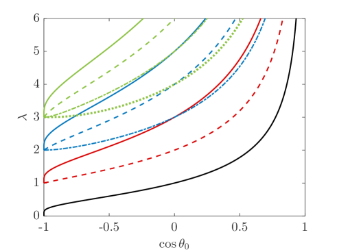
Figure 2: Dependence of polar eigenvalues (degrees) $\lambda_{i}^{m}$ for various azimuthal eigenvalues $m$s of a particle in a spherical box, confined by a cone of apex angle $2\theta_{0}$, on $w=\cos\theta_{0}$. Four lowest line bundles are shown (from bottom to top) $i=0$ (black), $i=1$ (red), $i=2$ (blue) and $i=3$ (green). The leftmost point of each bundle corresponds to the integer degree $\lambda_{i}^{m}=i=\ell$. For $w>-1$ each bundle splits into $i=\ell$ separate lines for $m=0,1,\dots,i=\ell$ with (top to bottom in each bundle) $m=0$ depicted as solid lines, $m=1$ – dashed lines, $m=2$ – dot-dashed lines, and $m=3$ – dotted line. When the cone becomes a plane ($w=0$) then the lowest line $\lambda_{0}^{0}$ corresponds to integer degree and order $(1,0)$, the second lowest line is $\lambda_{1}^{1}$ at $w=0$ geometry corresponds to $(2,1)$, while the third lowest point (intersection of $\lambda_{1}^{0}$ and $\lambda_{2}^{2}$ lines) corresponds to $(3,0)$ and $(3,2)$. The order $m$ remains constant along each of the lines, while the degree $\lambda$ changes.

As the angle of the cone changes, and the value of $w=\cos\theta_{0}$ varies between -1 and 1, the geometry of confinement changes between almost unconfined well with an excluded “needle” along the negative $z$ axis for $w=-1$, to an excluded cone along the negative $z$ axis ($-1<w<0$), to confinement by a plane, i.e., particle confined in the $z>0$ hemisphere ($w=0$), and to a particle confined inside a cone along the positive $z$ axis ($0<w<1$). If $w$ is changed continuously, the degree $\lambda^{m}_{i}$ also changes continuously as depicted in Fig. 2. For $w=-1$ we essentially have an unconstrained particle in a spherical box and $\lambda^{m}_{i}=i$ for $i=0,1,2,\dots$ independently of the values of $m$, as long as $i\geq|m|$. These are the $\ell$ values of the spherical harmonics, and each $\lambda^{m}_{i=\ell}=\ell$ is degenerate $2\ell+1$ times. This degeneracy is lifted once $w$ becomes larger than $-1$, except for two-fold degeneracy for $m\neq 0$ for $+m$ and $-m$ pairs, since $m$ appears only as $m^{2}$ in Eqs. (6) and (7). All $\lambda$s monotonically increase with $w$ eventually diverging in the $w\to 1$ limit. Thus every value of $\lambda_{i}(w=-1)$ splits into $i+1$ branches $\lambda^{m}_{i}$ corresponding to different $|m|$s. (We will refer to each such group of lines as a bundle.)

The divergence of the $\lambda_{i}^{0}$ lines in $w\to 1$ limit in Fig. 2 can be inferred from the properties of the zeros (roots) $\theta_{\lambda}^{(j)}$ ($j=1,2,\dots$) of $m=0$ Legendre functions $P_{\lambda}(\cos\theta)$ in the open interval $(0,\pi)$ of $\theta$s, i.e. the solutions of $P_{\lambda}(\cos\theta_{\lambda}^{(j)})=0$. (For $\ell<\lambda\leq\ell+1$ there are $\ell+1$ such roots.) In fact, all the curves in Fig. 2 have been constructed by choosing fixed $\lambda$ and fixed $m$ an finding all the roots, when every root belongs to a different curve in the figure, and then tracing the curves by gradually varying $\lambda$. For integer $\lambda$s only a discrete set of $\theta_{\lambda}^{(j)}$ can be accommodated, but for general $\lambda$s the roots can have any value. This statement can also be inverted to say that any value of $\theta_{0}$ can be a root corresponding to an infinite sequence of $\lambda_{i}^{0}$s or any vertical line in Fig. 2 intersects infinity of $\lambda_{i}^{0}$ curves. Several tight bounds on the roots are known – see, e.g., Ref. [26] and references therein. They can be used to produce large-$\lambda$ approximation $\lambda_{i}^{0}\approx\pi a_{i}/\theta_{0}$, with $i+1/2<a_{i}<i+1$, where the bounds on $a_{i}$ are derived from the bounds on the position of $(i+1)$th root. (Strictly speaking, the bounds on the roots in [26] have been derived for integer $\lambda$s, but for small $\theta_{0}$ and large $\lambda$ they can be used for noninteger $\lambda$s.) Since for small $\theta_{0}$, we can approximate $\theta_{0}\approx\sqrt{2(1-w)}$, and the functional dependence of the branches becomes $\lambda_{i}^{0}\approx\pi a_{i}/\sqrt{2(1-w)}$, thus explaining the divergences seen in Fig. 2. The bounds on the coefficients $a_{i}$ also ensure that the different branches $\lambda_{i}^{0}$ do not intersect. (Non-intersection of $\lambda_{i}^{0}$ lines is also ensured by the fact, that an intersection would create a multiple root of $P_{\lambda}$ thus contradicting the known fact that all their roots are simple.)

From the definition of associated Legendre functions $P_{\lambda}^{m}$ via derivatives of regular ($m=0$) Legendre functions $P_{\lambda}$, or from standard recurrence relations between the functions [27], one finds that

$$P_{\lambda}^{m+1}=-\sqrt{1-x^{2}}\frac{dP_{\lambda}^{m}}{dx}+\frac{mx}{\sqrt{1-x^{2}}}P_{\lambda}^{m}\ .$$ (8)

At two consecutive zeros (simple roots) of $P_{\lambda}^{m}$ the second terms on the right hand side of Eq. (8) vanish, while the first terms (the derivatives) have opposite signs, and therefore $P_{\lambda}^{m+1}$ will have opposite signs at those points. Thus, the zeros of $P_{\lambda}^{m+1}$ lie in between the zeros of $P_{\lambda}^{m}$. Consequently, the branch of $\lambda_{i}^{m}$ in Fig. 2 will be locked between branches $\lambda_{i}^{m-1}$ and $\lambda_{i-1}^{m-1}$, if they both exist, and will not intersect with them. Thus $m=1$ branches will be between $m=0$ branches, and $m=2$ branches will be between $m=1$ branches, etc. (However, $m=2$ branch can intersect $m=0$ branch, as can be seen in the intersection of $\lambda_{3}^{2}$ and $\lambda_{2}^{0}$ lines in Fig. 2.) Nevertheless, it means that lines $\lambda_{i}^{m}$ with any $m$ diverge as $1/\sqrt{1-w}$ for $w\to 1$, i.e. have the same divergence as $m=0$ branches. At every integer level $\lambda=\ell$, the horizontal line in Fig. 2 will cut $\ell-m$ branches with that particular $m$, since this is the number of zeros of $P_{\ell}^{m}$ in the open interval $(-1,1)$ of $w$. (This excludes extra zero at $w=-1$). For a noninteger $\lambda$ between some $\ell$ and $\ell+1$, the number of such intersections is $\ell-m+1$.

The eigenfunctions must vanish on the cone boundaries, even in the limit where the excluding cone becomes needle-like along the negative $z$ axis and, eventually, just a line for $w\to-1$. For $m\neq 0$ the polar eigenfunction of an unrestricted sphere $P_{\ell}^{m}$ vanishes at $\theta=\pi$ and therefore $P_{\lambda}^{m}$ naturally approaches $P_{\ell}^{m}$ as $\theta_{0}$ approaches $\pi$. Consequently, all $m\neq 0$ curves in Fig. 2 approach $w=-1$ points linearly. This is not the case for $m=0$, where $P_{\ell}^{0}$ does not vanish at $\theta=\pi$, and differs from $P^{0}_{\lambda}(\cos\theta_{0})=0$ for $w=\cos\theta_{0}=-1+\epsilon$, with $0<\epsilon\ll 1$. As $w$ approaches $-1$ the restricted and unrestricted solutions become almost identical everywhere except for a very narrow region around the negative $z$ axis, that remains present although its volume vanishes. This behavior is reflected in the fact that the $\lambda_{i=\ell}$ approaches its limiting value $\ell$ almost vertically: From the asymptotic forms of $P_{\lambda}^{0}$ near the singularity [28] one finds that for $w$ close to $-1$ the eigenvalue $\lambda^{0}_{i=\ell}\approx\ell-1/\ln(1+w)$.

To gain some intuition into the behavior of the curves in Fig. 2 we examine the relations between the eigenstates of unconfined particles in a spherical box ($w=-1$) and particles confined in a hemisphere ($w=0$). We note, that $\lambda$s are integers and with significant degeneracy for $w=-1$, but also for $w=0$ the $\lambda$s are integers, and there is some degeneracy due to intersections of different branches. In the former case the polar eigenvalues $\ell=0,1,\dots$, are degenerate $2\ell+1$ times, since for each $\ell$ we have $m=0,\pm 1,\dots,\pm\ell$. Spherical harmonics $Y_{\ell}^{m}$ can also be used to build the eigenstates of a hemisphere. We note that equality $P_{\ell}^{m}(\cos\theta_{0}=0)=0$ is valid when $\ell$ and $m$ have opposite parity. Thus almost half of the eigenfunctions of an unrestricted sphere vanish on the plane $\theta_{0}=\pi/2$ (or $z=0$) and can be used as a set of angular functions for hemisphere. Thus we have eigenfunctions and eigenvalues with $(\ell,m)=(1,0),\ (2,\pm 1),\ (3,0),\ (3,\pm 2),\dots$ The seeming reduction in the number of the eigenstates reflects the decrease in the volume of the system. We can now observe how the lowest branch that begins with $\lambda^{0}_{0}(w=-1)=0$, which corresponds to $(\ell,m)=(0,0)$ state of the complete sphere, increases with increasing $w$ and reaches $\lambda^{0}_{0}(w=0)=1$, which corresponds to $(\ell,m)=(1,0)$ eigenstate of the hemisphere. Similarly, the $m=1$ branch of $\lambda^{1}_{1}(w=-1)=1$ which corresponds to $(\ell,m)=(1,1)$ of a complete sphere increases and reaches value $\lambda^{1}_{1}(w=0)=2$, which corresponds to $(\ell,m)=(2,1)$ eigenstate of the hemisphere. The $m=0$ branch that also begins at $\lambda^{0}_{1}(w=-1)=1$, which corresponds to $(\ell,m)=(1,0)$ of a complete sphere reaches value $\lambda^{0}_{1}(w=0)=3$, which corresponds to $(\ell,m)=(3,0)$ eigenstate of the hemisphere. At $w=0$ the latter branch intersects $m=2$ branch that started at $\lambda^{2}_{2}(w=-1)=2$ and reached $\lambda^{2}_{2}(w=0)=3$, which corresponds to $(\ell,m)=(3,2)$ eigenstate of the hemisphere, and therefore completes the eigenstate mentioned before with $m=0$. Thus, increase in $w$ causes “reordering” of the eigenstates. There are additional intersections of different branches, corresponding to a variety of cone angles $\theta_{0}$. Those, however, are accidental degeneracies of unrelated states.

The line intersections in Fig. 2 described in the previous paragraph are in line with the theorem [29] that two associated Legendre functions $P_{\ell}^{m}(w)$ and $P_{\ell}^{m^{\prime}}(w)$ with integer degrees and orders and $|m|\neq|m^{\prime}|$ have no common zeros with exception of the case when $\ell$ and $m$ have opposite parity, as well as $\ell$ and $m^{\prime}$ have opposite parity, in which case they have common zeros at $w=0$. This exactly describes the intersections at $w=0$ in Fig. 2. At the same time, it means that there can be no other intersections at integer $\lambda$s. Indeed, the accidental intersection of $\lambda_{3}^{3}$ and $\lambda_{2}^{0}$ lines in Fig. 2 appears at non-integer $\lambda$ slightly larger than 3.

The radial part $R(r)$ of the eigenfunctions of Eq. (5) is a solution of the equation

$$\frac{1}{r^{2}}\frac{d}{dr}\left(r^{2}\frac{dR}{dr}\right)+\frac{\lambda(\lambda+1)}{r^{2}}R=\left[E-U(r)\right]R,$$ (9)

where the radial component $U(r)$ of the potential $V({\bf r})$ vanishes inside the well, and only manifests by the boundary condition $R(r=1)=0$. This is correct both in the absence and the presence of the confining cone. We note that the equation only depends on the polar eigenvalue $\lambda$ but not on $m$, although the actual value of $\lambda$ may depend on $m$. This equation is solved by the spherical Bessel functions $j_{\lambda}(\sqrt{E}r)$, so that the complete eigenfunctions are $\psi\left(r,\theta,\varphi\right)\propto j_{\lambda}\left(\sqrt{E}r\right)P_{\lambda}^{m}\left(\cos\theta\right)e^{im\varphi}$. By imposing the boundary condition $j_{\lambda}(\sqrt{E})=0$, we find the energy spectrum of the system

$$E_{n}(\lambda)=\alpha_{n}^{2}(\lambda),$$ (10)

where $\alpha_{n}(\lambda)$ is the $n$th zero of $j_{\lambda}(x)$. Figure 3 shows part of the energy spectrum as function of $\cos\theta_{0}$ for different values of $n$, $\lambda$ and $|m|$. Since the eigenenergies directly depend only on $\lambda$, the Fig. 3 slightly resembles Fig. 2. In particular degeneracies (accidental or not) seen in Fig. 2 are “reproduced” in the energy lines. To facilitate comparison of these two figures, we employed the same coloring and line-type scheme for the graphs: the energy line types and colors are identical to lines types and colors used to described $\lambda$s for which those energies were calculated. However, since every specific value of $\lambda$ produces an infinite series of roots $\alpha_{n}(\lambda)$, with $n=1,2\dots$, every single line in Fig. 2 produces many lines in Fig. 3. They are distinguished in Fig. 3 by line thickness where $n=1$ corresponds to the thickest lines, and the thickness decreases with increasing $n$. Besides the energy degeneracies originating in the degeneracies of $\lambda$s, there are additional accidental degeneracies when roots of different order belonging to different $\lambda$s coincide. Due to simple relation between the energies and $\lambda$s in Eq. (10) the properties of $\lambda$s in $w\to-1$ and $w\to 1$ limits are partially (qualitatively) mimicked in the energy spectrum.

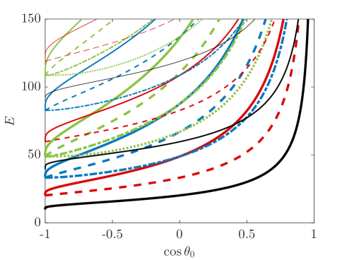
Figure 3: The energy $E$ spectrum as function of $w=\cos\theta_{0}$. For each $\lambda$ shown in Fig. 2 there is an infinite sequence of roots $n=1,2,\dots$ shown with different line thicknesses, the very thick (lowest) line ($n=1$), intermediate thickness (higher) line ($n=2$), thin (highest) line ($n=3$), while the line styles and colors are the same is in Fig. 2. Since the roots of Bessel functions depend only on the values of $\lambda$ every bundle of $\lambda$s in Fig. 2 creates multiple similar bundles of energy lines in this figure. Degeneracies of $\lambda$ lines in Fig. 2 translate into energy degeneracies in this figure. Additional accidental energy degeneracies are created by intersection energy lines belonging to different $n$s.

Since for large $\lambda$ the first root $\alpha_{1}(\lambda)\sim\lambda$ [30], the ground state energy will (due to Eq. (10)) diverge in the $w\to 1$ limit as $(\lambda_{0}^{0})^{2}\sim 1/\theta_{0}^{2}\sim 1/(1-w)$. The same conclusion can be reached from Heisenberg’s uncertainty principle, since for small $\theta_{0}$ the confining dimension in the sphere of radius $a$ constrained by the cone is $a\theta_{0}$ leading to uncertainty in momentum of order $\hbar/a\theta_{0}$, which corresponds in our dimensionless units to energy $E\sim 1/\theta_{0}^{2}$.

3 Weyl relations in a confined infinite well

As can be seen in Fig. 3 the eigenenergies corresponding to a particular branch increase with increasing confinement, and the number of eigenstates ${\cal N}(E)$ with energies below a certain value $E$ decreases. The exact ${\cal N}(E)$ in a box of an arbitrary shape is a step-wise function, which jumps upwards by an integer amount whenever an eigenenergy is encountered. The size of the jump is the degeneracy of that energy level. For more than a century Weyl and his successors developed a smooth function ${\cal N}_{W}(E)$ approximating ${\cal N}(E)$, which in $d$ dimensions has the form ${\cal N}_{W}=a_{1}E^{d/2}+a_{2}E^{(d-1)/2}+a_{3}E^{(d-3)/2}+\dots$. (For an overview see Refs. [31, 32, 33].) The expression for ${\cal N}_{W}$ is rather general and requires surprisingly little information about the system. However, some uncertainty exists both regarding the exact conditions for the validity of such expressions and the behavior of the remainder

$$r(E)\equiv{\cal N}(E)-{\cal N}_{W}(E).$$ (11)

The subject has been extensively studied for a particle in a square (cubic) box in 2D (3D), where the problem of number of states is reduced to the counting of number of square (cubic) lattice points $\cal N$ within a circle (sphere) of radius $R$. (The radius $R$ is proportional to $\sqrt{E}$ in the quantum problem.) One can easily produce a continuous estimate ${\cal N}_{W}$ for such geometries [31]. However, the estimate of the remainder $r(E)$ dates back to “Gauss circle problem” (in 2D case), and has a long history of bounds [31] that are specific to the shapes of the quantum boxes.

Robinett studied a circular box in 2D confined in a sector [34]. When the opening angle of the sector is changing, the area and the perimeter of the confining box both change, but they are are not proportional to each other. The structure of the eigenfunctions is relatively simple, since the azimuthal (angular) eigenstates are simple sine functions. This work demonstrated the validity of two-dimensional (2D) Weyl formula for the system. Particularly enlightening in that study is the comparison of full (unconstricted) circle, with a circle when the the sector has a angle of $2\pi$, i.e., degenerates into a single excluding radius line, and with the sector that has opening angle $\pi$, i.e., the particle is restricted to a semi-circular box. Our problem of a spherical box restricted by a cone is the 3D generalization of the same problem. However, as explained in the previous section, already the determination of the polar degrees $\lambda$ as functions of the cone apex half-angle $\theta_{0}$ had to be performed numerically, followed by a solution of the radial eigenvalue equation determining the eigenenergies $E$, that are related to the numerically known roots of Bessel functions. Nevertheless, we verified the accuracy of Weyl expressions for several angles $\theta_{0}$. Unlike the 2D problem, the case corresponding to $\theta_{0}=\pi$, i.e., when the cone becomes an excluded needle, the spectrum coincides with that of completely unrestricted sphere, i.e., in 3D the excluded zero-width radial line does not modify the energy spectrum. In this section we present in detail comparison of the $\theta_{0}=\pi$ and $\theta_{0}=\pi/2$ cases, i.e., a complete sphere and a hemisphere. The angular parts of the eigenfunctions in these cases are represented by integer $\ell$s and $m$s and provide intuitive insights into the properties of Weyl formula.

The fact that density of states per unit volume in 3D system exists independently of the overall shape of the system, i.e., the leading term in the number of states ${\cal N}$ is proportional to the system volume $\cal V$, was implicit in the calculations of black body radiation or counting mechanical oscillatory modes in a solid already in the late 19th and early 20th centuries. Similar problem appears in the statistics of the eigenenergies of Schrödinger equation for a particle in a box. Mathematically, this is a scalar Laplacian eigenvalue problem of determining the number of eigenstates up to a certain value $E$. (It is related, but not identical, to nonscalar problems, such as classical electromagnetic or elastic waves, where $E$ is replaced by squared wavevector.) It has been formally proven by Weyl that to the leading order $\cal N$ is proportional to the system volume $\cal V$. In our dimensionless variables this number of states (for a scalar problem in 3D) is ${\cal T}_{1}=({\cal V}/6\pi^{2})E^{3/2}$. Our choice of unit length scale $a$ does not affect the formula, because a choice of different length scale $a$, modifies values of ${\cal V}$ and $E$, while making no change in the coefficient of the formula. Similarly, the change in the shape of the box does not influence this expression. In our examples of the sphere- and hemisphere-shaped boxes the unit length defined as the radius of the sphere, and the system volumes will be ${\cal V}_{\Circle}=4\pi/3$ and ${\cal V}_{\!\!\Rightcircle}=2\pi/3$, respectively.

For finite systems boundaries introduce subleading corrections to the total number of states. The corrections depend on the type of boundary conditions (b.c.) imposed on the wavefunction, such as function vanishing on the boundary (Dirichlet b.c.), or normal derivative of the function vanishing on the boundary (Neumann b.c.), or linear combination of the function and its normal derivative vanishing (Robin b.c.) [35] conditions. In 1913 Weyl conjectured [36] that for smooth bounding surfaces the correction to the number of eigenstates in the Laplacian problem with Dirichlet b.c. is proportional to the surface area ${\cal S}$ and is given by ${\cal T}_{2}=-({\cal S}/16\pi)E$. (The coefficient in this expression depends on b.c. [35] and, in particular, for Neumann b.c. it is the same expression but with an opposite sign.) In our examples of sphere- and hemisphere-shaped boxes the surface areas are ${\cal S}_{\Circle}=4\pi$ and ${\cal S}_{\!\!\Rightcircle}=3\pi$, respectively.

Even smaller correction originates from the shape (“curvature”) of the surface, and is given by ${\cal T}_{3}=({\cal C}/6\pi^{2})E^{1/2}$. The differentiable parts of the surface where two main radii of curvature $R_{1}$ and $R_{2}$ can be defined contribute to $\cal C$ the integral of mean curvature $\int dS\frac{1}{2}\left(1/R_{1}+1/R_{2}\right)$. If the surface contains sharp wedges, then their contribution depends on the wedge angle [31], and in particular $90^{\circ}$ wedges contribute to ${\cal C}$ amount $(3\pi/8){\cal L}$, where $\cal L$ is the total length of such wedges. In our examples for a spherical box we have only the curvature term: since the mean curvature of the sphere of unit radius is 1, the total curvature contribution is ${\cal C}_{\Circle}=4\pi$. For the hemisphere the nonvanishing curvature contributes $2\pi$, while the $90^{\circ}$ edge of length $2\pi$ contributes another $3\pi^{2}/4$, leading to total ${\cal C}_{\!\!\Rightcircle}=2\pi+3\pi^{2}/4$.

By combining the volume, surface area and “curvature” terms of Weyl function we get the following expression for the number of states [31]

$${\cal N}_{W}(E)={\cal T}_{1}+{\cal T}_{2}+{\cal T}_{3}+\dots=\frac{{\cal V}}{6\pi^{2}}E^{3/2}-\frac{{\cal S}}{16\pi}E+\frac{{\cal C}}{6\pi^{2}}E^{1/2}+o(E^{1/2}),$$ (12)

In the specific cases of sphere and hemisphere, these can be written as

$${\cal N}_{W\Circle} =\frac{2}{9\pi}E^{3/2}-\frac{1}{4}E+\frac{2}{3\pi}E^{1/2}+\dots$$ (13)

$${\cal N}_{W\!\!\Rightcircle} =\frac{1}{9\pi}E^{3/2}-\frac{3}{16}E+\left(\frac{1}{3\pi}+\frac{1}{8}\right)E^{1/2}+\dots$$ (14)

The validity of these expressions is demonstrated in Fig. 4(a) which has been obtained by numerically enumerating the total number of states for each energy $E$. The figure presents the exactly measured ${\cal N}(E)$ both for the sphere and the hemisphere and compares the exact results with Weyl functions in Eqs. (13) and (14). Each of the latter equations are shown in three approximate forms: solid line depicts only the first Weyl terms, the dashed line depicts first two Weyl terms, and the dotted line depicts three terms. While two-term lines represent strong improvement in the correspondence with measured $\cal N$ over the single-term lines, the three-term lines are barely distinguishable from two-term lines in Fig. 4(a). Moreover, the fluctuations of the remainder $r(E)$ defined in Eq. (11) increase with $E$, and their departure from the continuous curves is larger than the third term correction to ${\cal N}_{W}$. (A meaningful comparison and validation of the third term can be done only if the exact stepwise curve $\cal N$ is smoothed by an averaging procedure [31].) The extent of fluctuations can be characterized by a bound $|r(E)|<cE^{\beta}$, where $c$ and $\beta$ are some constants. For a cubic box there exist some theoretical bounds on $\beta$, but no such bounds are known for a spherical box. By numerically examination the $|r(E)|$ graphs in the range $E<4000$, we note that all data points of a sphere fit under a curve with $\beta=1/2$, and $c\approx 3.2$, while for the hemisphere we have the same $\beta$ with twice smaller $c$. (However, these numbers are just the “ballpark” estimates of a “random” function in a limited energy range.)

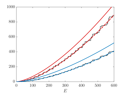
(a)

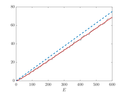
(b)

Figure 4: (a) The exact numbers of eigenstates (step-wise solid black lines) for sphere (top bundle of lines) and hemisphere (lower bundle of lines) as functions of the energy $E$. The exact results are compared with Weyl approximate continuous lines for a sphere (red) and a hemisphere (blue) as in Eqs. (13) and (14), where in each bundle the top solid lines show only the first (leading) term for both geometries, the lowest dashed lines show two first terms, and a dotted lines slightly above the dashed lines show all three terms. (b) The exact difference between the numbers of steps in a sphere and twice the number of states in a hemisphere (step-wise solid lines) ${\cal N}_{\Circle}-2{\cal N}_{\!\!\Rightcircle}$ as function of the energy $E$. It is compared with the Weyl estimates of the difference. The leading terms in Weyl formulas cancel out, and the dashed (blue) line represents the difference of second terms ($\frac{1}{8}E$), while the dotted (red) line represents the difference of second and third terms, i.e., $\frac{1}{8}E-\frac{1}{4}E^{1/2}$.

As explained in the previous section the eigenstates of a complete sphere and a hemisphere can be represented by integer $l$s, and the energies become independent of $m$. Therefore both the exact $\cal N$s and their Weyl approximations ${\cal N}_{W}$ are simply related. For a complete sphere each $\ell$ state is $2\ell+1$ times degenerate, while in hemisphere the parity of $\ell$ and $m$ must be opposite, and therefore each $\ell$ state is degenerate $\ell$ times. Let ${\cal N}_{\ell}(E)$ be a number of zeroes of the spherical Bessel function $j_{l}(x)$ up to certain maximal value $x=\sqrt{E}$, which via relation (10) is the number of distinct eigenenergies, up to energy $E$. (This function ignores the degeneracies of the energies.) Then

$${\cal N}_{\Circle}(E) =\sum_{\ell}(2\ell+1){\cal N}_{\ell}(E),$$ (15)

$${\cal N}_{\!\!\Rightcircle}(E) =\sum_{\ell}\ell{\cal N}_{\ell}(E).$$ (16)

(The summation over $\ell$ is finite since starting with some $\ell$ there are no more eigenstates with energies lower than $E$.) It is known [30] that for large $\ell$s the density of zeros of spherical Bessel function $j_{\ell}$ approaches a constant: $\rho(x)=(1/\pi)(1+(\ell+1/2)^{2}/x^{2})^{1/2}$ for $x>\ell+1/2$. Consequently, for a given $\ell$ the number of roots up to energy $E$ will be (to the leading order and neglecting prefactors) ${\cal N}_{\ell}(E)\sim(\sqrt{E}-\ell)$. Both ${\cal N}_{\Circle}(E)$ and ${\cal N}_{\!\!\Rightcircle}(E)$ in Eqs. (15) and (16) include $\sum_{\ell}\ell{\cal N}_{\ell}(E)\sim\int^{\sqrt{E}}d\ell\ell(\sqrt{E}-\ell)\sim E^{3/2}$, thus explaining the leading terms in the Weyl relations.

It is interesting to consider the difference between the number of states in a sphere and twice the number of states in a hemisphere. From Eqs. (15) and (16) ${\cal N}_{\Circle}(E)-2{\cal N}_{\!\!\Rightcircle}(E)=\sum_{\ell}{\cal N}_{\ell}(E)$. Not surprisingly, this difference cancels out the terms proportional to volume, and we can expect to have the leading term proportional to $E$. Indeed from the approximate value of ${\cal N}_{l}$ we find that $\sum_{\ell}{\cal N}_{\ell}(E)\sim\int^{\sqrt{E}}d\ell(\sqrt{E}-\ell)\sim E$. Analogously, by subtracting Weyl functions of these systems we get ${\cal N}_{W{\Circle}}(E)-2{\cal N}_{W{\!\!\Rightcircle}}(E)=\frac{1}{8}E-\frac{1}{4}E^{1/2}$. Figure 4(b) depicts the exact difference between the numbers of states by a step-wise solid line. This result is compared with the difference obtained from Weyl expressions truncated at the second term (dashed line) and including also the third term (dotted line). We note an excellent agreement between the exact results and the predictions of Weyl functions. Such clarity of the result is a consequence of very small remainders $r(E)$ which are significantly smaller than were seen in Fig. 4(a). In fact in the range of $E<4000$ we found that $|r(E)|<4$, i.e., it does not increase with $E$. Apparently, since this is the sum of ${\cal N}_{l}$s that does not account for degeneracies of the eigenstates, the fluctuations are significantly suppressed. The accuracy of the third term in Weyl equation can be clearly seen in this picture. It seems that the entire increase in the fluctuations $|r(E)|$ in Fig. 4(a) was caused by the growing degeneracy of the high energy eigenstates.

4 Finite spherical well bounded by a cone

It is well known in quantum mechanics that purely attractive potential in $d=1$ always has a bound state [37], and for a sufficiently deep well it may have many bound states. (There is also a slightly more relaxed criterion guaranteeing the presence of bound states [38, 39, 40].) Similar situation also exists in 2D, where the bound state can always be found [41]. If space dimension $d$ is considered as continuous variable, it can be shown that this property disappears when $d>2$ [42]. In particular, in 3D the presence or absence of the bound state depends on the shape and depth of the binding potential. However, for potentials that have repulsive parts, such as infinite barriers, the bound states are not necessarily present, and 3D case may resemble lower-dimensional situations.

In this section we consider a finite spherical well of radius $a=1$ with depth $U_{0}$ below zero potential outside the well, measured in the same dimensionless units as in Sec. 2. The finite well is bounded by a circular cone with an apex angle $2\theta_{0}$ such that

$$V\left(\text{{r}}\right)=\begin{cases}-U_{0},&r<1,\,\theta<\theta_{0},\\ 0,&r>1,\,\theta<\theta_{0},\\ \infty,&\text{otherwise}.\end{cases}$$ (17)

This system admits both bound ($E<0$) and unbound ($E>0$) eigenstates, and we will examine the transitions between them for various well depths and apex half-angles $\theta_{0}$. Since the problem permits the same variable separation as in the infinite well case discussed in Sec. 2 the angular (polar and azimuthal) dependence of both bound and unbound states inside and outside the spherical well are determined by the cone and are identified by the same $\lambda_{i}^{m}$s corresponding to a particular $\theta_{0}$, that were depicted in Fig. 2 and explained in detail in Sec. 2.

The radial component of the wavefunctions $R(r)$ also satisfies the same Eq. (9) as for infinite potential well described in Sec. 2 but with the radial part of the potential

$$U(r)=\begin{cases}-U_{0},&r<1,\\ 0,&r>1.\end{cases}$$ (18)

Within the regions that the potential is constant (either $-U_{0}$ or 0), Eq. (9) can be solved by spherical Bessel functions of the first and second kind, $j_{\lambda}$ and $n_{\lambda}$, respectively, when the eigenenergy exceeds the potential, and modified spherical Bessel functions $i_{\lambda}$ and $\kappa_{\lambda}$ for eigenenegies below the the potential. The spherical Bessel functions are related to the regular (nonspherical) Bessel functions (denoted by the capital letters) by $j_{\lambda}(x)=\sqrt{\pi/2x}J_{\lambda+1/2}(x)$, $\kappa_{\lambda}(x)=\sqrt{\pi/2x}K_{\lambda+1/2}(x)$, and the same for other function pairs. We note, that the regular Bessel functions $J_{\lambda}$, $N_{\lambda}$, $I_{\lambda}$, and $K_{\lambda}$ solve analogous radial equation in 2D [10], and some of the results presented below resemble solutions of 2D problem, with $\lambda$ shifted by $1/2$.

For bound states ($-U_{0}<E<0$) the radial part of the wavefunction is proportional to $j_{\lambda}(kr)$, with $k=\sqrt{E+U_{0}}$ inside the well, while $n_{\lambda}$ is dismissed since it diverges at the origin, and $\kappa_{\lambda}(qr)$, with $q=\sqrt{-E}$ outside the well, while $i_{\lambda}$ is dismissed since it diverges at $r\to\infty$. Thus the wavefunction has the form

$$\psi_{n\lambda m}({\bf r})\propto P_{\lambda}^{m}\left(\cos\theta\right)e^{im\varphi}\begin{cases}j_{\lambda}\left(kr\right),&r<1,\\ \kappa_{\lambda}\left(qr\right),&r>1.\end{cases}$$ (19)

Since the radial part of the Schrödinger equation is second order differential equation with a potential which is a stepfunction ar $r=1$, both the wave function and its derivative must by continuous at $r=1$, although the slope of the derivative changes at $r=1$ leading to a finite jump in the second derivative, and therefore

$$\frac{kj^{\prime}_{\lambda}(k)}{j_{\lambda}(k)}=\frac{qk^{\prime}_{\lambda}(q)}{\kappa_{\lambda}(q)}\ ,$$ (20)

where prime denotes derivative of the function. The overall prefactor of the functions is determined from normalization conditions. Since the value of $\lambda=\lambda_{i}^{m}$ was determined form the angular equation, and $U_{0}$ is implicit in the definition of $k$, the only unknown parameter in Eq. (20) is energy $E$ that determines both $k$ and $q$. The possible values of $E$ satisfying this equation are the eigenenegies of the bound eigenstates. Interestingly enough, if we express the spherical Bessel functions via regular ones and perform the derivatives in the numerators of all the functions, Eq. (20) becomes the relation

$$\frac{kJ^{\prime}_{\lambda+1/2}(k)}{J_{\lambda+1/2}(k)}=\frac{qK^{\prime}_{\lambda+1/2}(q)}{K_{\lambda+1/2}(q)},$$ (21)

which is exactly the 2D continuity relation for a circular well contained by a sector, but with a shift $\lambda\to\lambda+1/2$ [10].

For various $\lambda_{i}^{m}$s there can be several, one or no bound eigenenergy solutions of Eqs. (20) or (21). As the well becomes shallower ($U_{0}$ decreases) the number of bound states also decreases, until only one bound eigenstate corresponding to $\lambda=\lambda_{0}^{0}$ remains with some eigenenergy $E_{0}<0$. When the well depth decreases to some critical $U_{c}$ the bound states disappear altogether. When $E_{0}\to 0$, then $q\to 0$, and the right hand side of Eq. (21) approaches $-(\lambda+1/2)$ [10], while in the left hand side $k\to\sqrt{U_{c}}$. The relation for critical depth of the well is

$$\frac{\sqrt{U_{c}}J^{\prime}_{\lambda+1/2}(\sqrt{U_{c}})}{J_{\lambda+1/2}(\sqrt{U_{c}})}=-(\lambda+1/2),$$ (22)

which by using recurrence relations between Bessel functions and their derivatives [43] reduces to

$$J_{\lambda-1/2}(k)=0,\ {\rm or}\ \ j_{\lambda-1}(k)=0,$$ (23)

with $k=\sqrt{U_{c}}$. Thus $U_{c}$ is simply the square of the first zero of these functions. As can be seen in Fig. 2 for each $\theta_{0}$ (or $w=\cos\theta_{0}$) there exists an infinite sequence of $\lambda_{i}^{m}$s. Since, $U_{c}$ represents the case when the last remaining (ground) eugenstate has zero energy, we must use the lowest $\lambda=\lambda_{0}^{0}$, and therefore

$$U_{c}=\alpha^{2}_{1}(\lambda_{0}^{0}-1).$$ (24)

(To compare this result with the 2D case, see Eq. (16) in Ref. [10].) Fig. 5a depicts the dependence of the critical depth $U_{c}$ on the cone apex half-angle $\theta_{0}$. For small $\theta_{0}$ the confinement is strong and large $U_{c}$ is required. Indeed, for large $\lambda$ the first root of $J_{\lambda}$ is approximately $\lambda$, and therefore $U_{c}\sim\lambda^{2}\sim 1/\theta_{0}^{2}$. As $\theta\to\pi$ the critical depth drops to the critical value of an unconstrained spherical well.

Equations (22) and (23) relied solely on the assumption that the energy of the eigenstate vanishes and were not specific to the case of single remaining bound state. We might consider situations when a vanishing energy eigenstate appears for deeper wells, when additional negative energy bound states are still present. For each $\lambda_{i}^{m}$ there is an infinite amount of such well depths corresponding to different zeros of the same Bessel function:

$$U_{0}^{(i,m,n)}=\alpha^{2}_{n}(\lambda_{i}^{m}-1).$$ (25)

The critical $U_{c}$ in Eq. (24) is just the smallest depth in the infinite sequence of values in Eq. (25).

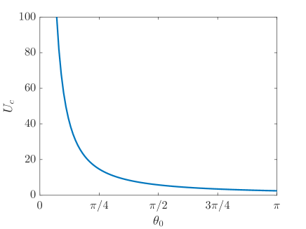
(a)

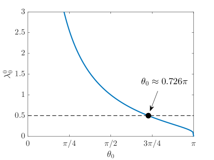
(b)

Figure 5: (a) The critical depth of the well $U_{c}=\alpha_{1}^{2}(\lambda_{0}^{0}-1)$ (see text) as a function of the cone apex half-angle $\theta_{0}$. (b) The ground-state angular degree $\lambda_{0}^{0}$ as a function of the cone apex half-angle $\theta_{0}$. The special value $\lambda_{0}^{0}=1/2$ is shown by a dashed line.

5 Critical exponents

The radial part of the wavefunction of a bound state is characterized by energy $E<0$ and the corresponding $q=\sqrt{-E}$ outside the well is described by $\kappa_{\lambda}(qr)$, where the polar constant (degree) $\lambda=\lambda_{i}^{m}$, while the energy (or $q$) is obtained from one of the solutions of Eq. (20). For $qr\gg 1$, the function $\kappa_{\lambda}(qr)\sim\frac{1}{qr}e^{-qr}$, i.e., it has a typical decay (localization) length $\xi\equiv 1/q=1/\sqrt{-E}$. As the energy of a specific eigenstate approaches 0 the length $\xi\to\infty$. Eigenstates with zero binding energy for several potential types have been studied in Refs. [44, 45], and became parts of textbooks (see, e.g., Ref. [1]). For the $E=0$ eigenstate the radial part of the eigenfunction becomes

$$R(r)\propto\begin{cases}j_{\lambda}\left(kr\right),&r<1,\\ 1/r^{\lambda+1},&r>1,\end{cases}$$ (26)

where the continuity condition at $r=1$ in Eq. (20) is the same as in Eqs. (20-23). If we are considering the single surviving bound state, then $\lambda=\lambda_{0}^{0}$, $k=\sqrt{U_{c}}$, which is given by the critical value $U_{c}$ defined in Eq. (24). This case plays an especially important role, because in the analogy between quantum states and ideal polymers, the state of long polymer is dominated by the ground state of the quantum problem, and whether this state is bound or not determines whether the polymer is adsorbed or not to the attractive potential area. (See Sec. 6.) However, the argument presented here can also be applied for deeper potentials $U_{0}$ that support several bound states, for each case of the depth $U_{0}=U_{0}^{(i,m,n)}$ as defined in Eq. (25) for which a zero energy state appears. For simplicity, below we will mostly consider only a well slightly deeper than $U_{c}$ and admitting a single bound state.

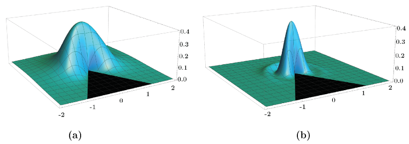
Figure 6: Probability density function $|\psi(r,\theta,\varphi=0)|^{2}$ (not normalized) for $\theta_{0}=5\pi/6\approx 0.833\pi$. The horizontal plane of the graph represents $\theta,r$ coordinate plane, i.e., a cut through $x-z$ plane of Cartesian coordinates. The excluded cone is represented by the darker area of the plane. Two cases with two different eigenenergies are shown: (a) $E=0$ eigenstate for $U_{0}=U_{c}\approx 4.740$, corresponding to $\lambda_{0}^{0}\approx 0.355$ with $\psi$ that decays as a power law $\sim 1/r^{1.355}$ outside the sphere, and therefore is not square-integrable. (b) Bound eigenstate with $E\approx-7.613$ corresponding to the second zero of the Bessel function for $U_{0}=40\approx 8.44U_{c}$ and the same $\lambda_{0}^{0}$, that decays exponentially for large distances. While this is the second state of $\lambda_{0}^{0}$, it is the sixth lowest state overall.

The normalization of the ground state requires the radial integration $\int r^{2}|\psi|^{2}dr$. If the radial part $R(r)$ of the eigenstate behaves at large distances as $1/r^{\lambda+1}$, the integral will only converge for $\lambda>1/2$. Figure 5(b) redraws the lowest branch $\lambda_{0}^{0}$ of Fig. 2 as a function of $\theta_{0}$. There is an entire region of this branch where $0<\lambda_{0}^{0}\leq 1/2$ corresponding $\pi>\theta_{0}>\theta_{c}\approx 0.726\pi$. In that region the normalization cannot be performed, and these $E=0$ energy states can be categorized as unbound states. Figure 6a depicts such a non-normalizable state for $U_{0}=U_{c}$ at large $\theta_{0}$. Interestingly enough, $E=0$ states corresponding to other branches of $\lambda$ spectrum always have $\lambda_{i}^{m}\geq 1$ and therefore are normalizable. For deep $U_{0}$ there may be other eigenstates corresponding to $\lambda_{0}^{0}$ and higher order zeros of of Bessel function, which also cannot be normalized at these angles. The bound state depicted in Fig. 6b corresponds (for large $U_{0}$ to the second zero of Bessel function for the same $\lambda_{0}^{0}$ is the eigenstate in Fig. 6a. The fact that it is the second zero can be seen in the single oscillation that performs the wavefunction inside the well. If $U_{0}$ is decreased, at some point the eigenenergy of this state will reach zero and it will resemble the behavior of the state in Fig. 6a but with larger $k$ in the $r<1$ region. Similar type of normalizability problem exists in 2D problem of a sector confining a circle. However, in 2D the borderline $\theta_{c}$ corresponds to the sector becoming a straight line, while in our case the special angle of $\theta_{c}$ has no “special” geometrical meaning.

For $U_{0}>U_{c}$ the ground state has finite $q$ and $\xi$ which we expect to vanish and diverge, respectively, as $U_{0}\to U_{c}$. When $\delta U\equiv U_{0}-U_{c}\ll U_{c}$, then $E$ is also small and we can expand both sides of Eq. (20) in these small quantities to find the dependence of $E$ on $\delta U$, and therefore the dependence of $\xi$ on $\delta U$. We denote the left hand side of Eq. (20) by ${\cal G}_{\text{L},\lambda}(k)\equiv kj^{\prime}_{\lambda}(k)/j_{\lambda}(k)$, and right hand side by ${\cal G}_{\text{R},\lambda}(q)\equiv q\kappa^{\prime}_{\lambda}(q/\kappa_{\lambda}(q)$. The expansion of the left hand side is given by [43]

$${\cal G}_{\text{L},\lambda}(k)={\cal G}_{\text{L},\lambda}\left(\sqrt{U_{c}+\delta U+E}\right)\approx-\lambda-1-\frac{1}{2}(E+\delta U),$$ (27)

while the form of the expansion of the right hand side depends on the value of $\lambda$ [43]:

$${\cal G}_{\text{R},\lambda}(q)={\cal G}_{\text{R},\lambda}\left(\sqrt{-E}\right)\approx\begin{cases}-\lambda-1-\frac{1}{2\left(\lambda-\frac{1}{2}\right)}\left(-E\right),&\lambda>\frac{1}{2},\\ -\frac{3}{2}+\frac{1}{2}\left(-E\right)\ln\left(-E\right),&\lambda=\frac{1}{2},\\ -\lambda-1-\frac{2^{-2\lambda}\pi}{\cos\left(\pi\lambda\right)\Gamma^{2}\left(\lambda+\frac{1}{2}\right)}\left(-E\right)^{\lambda+\frac{1}{2}},&0\leq\lambda<\frac{1}{2}.\end{cases}$$ (28)

By equating ${\cal G}_{\text{L},\lambda}={\cal G}_{\text{R},\lambda}$ we extract the dependence of $-E$ on $\delta U$, and consequently the $\delta U$-dependence of $\xi$, in the form $\xi\sim\delta U^{-\nu}$:

$$\xi\sim\begin{cases}\delta U^{-\frac{1}{2}},&\text{for}\,\lambda>\frac{1}{2},\\ \left|\ln\delta U\right|^{\frac{1}{2}}\delta U^{-\frac{1}{2}},&\text{for}\,\lambda=\frac{1}{2},\\ \delta U^{-\frac{1}{2\lambda+1}},&\text{for}\,0\leq\lambda<\frac{1}{2}.\end{cases}$$ (29)

For small angles $\theta_{0}$ (large $\lambda$) the critical exponent controlling the $\delta U$-dependence of $\xi$ is $\nu=1/2$. However for large enough angles $\theta_{0}>\theta_{c}$ the exponent $\nu=1/(2\lambda+1)$ becomes angle $\theta_{0}$-dependent and reaches 1 when $\theta_{0}\to\pi$. Note that the transition between angle-dependent and angle-independent regimes occurs when at $\theta_{0}=\theta_{c}$ when $\lambda=1/2$.

The above derivation could be repeated also in the situation when $U_{0}$ approaches any of the $U_{0}^{(i,m,n)}$ defined in Eq. (25), and the Eq. (29) is valid with $\delta U\equiv U_{0}-U_{0}^{(i,m,n)}$. However, the only $\lambda$ capable of having values below $1/2$ is $\lambda_{0}^{0}$. Therefore, the usual value of the exponent is $\nu=1/2$, with exception of the cases of $\theta_{0}>\theta_{c}$ and $\lambda_{0}^{0}<1/2$, corresponding to various order zeros, i.e., $U_{0}^{(0,0,n)}$ with $n=1,2,\dots$

6 Discussion

Some of the results derived in our work resemble the regular solutions of a particle in a spherical box or a particle in a finite potential well in the absence of the cone. However, in the spherically-symmetric case the degree $\ell$ is integer, and many of the effects described in this work are absent. For instance, the discussion of $E=0$ eigenstates in Refs. [44, 45] omits the trivial $\ell=0$ case, and proceeds to discuss $\ell\geq 1$ case, when the interesting effects and the qualitative change in the behavior, such as lack of integrability of the $E=0$ state, appears for noninteger $\lambda\leq 1/2$.

In the mapping between the quantum and the ideal polymer problems [9] the quantum potential is replaced by the actual potential divided by $k_{B}T$. The probability density of the end-point of an $N$-monomer polymer is given by a superposition of the ${\bf r}$-dependent quantum eigenstates multiplied by ${\rm e}^{-EN}$, where $E$ is energy of a particular state and the exponent replaces the time-depended oscillatory term of the quantum mechanics. For large $N$ the state with the smallest $E$ will dominate the density distribution and its localization length $\xi$ will be the spatial extent of the polymer. Since $\xi$ is finite only for the bound quantum states, the absence or presence of the polymer adsorption is related to the existence of the bound state. The effective depth of the “polymer potential” is varied by changing $T$, and when $T$ approaches the critical adsorption temperature $T_{a}$ the effective value $U$ of the quantum problem approaches $U_{c}$ and $\delta U\sim(T_{a}-T)$. In this situation Eq. (29) can be re-written in the form

$$\xi\sim\begin{cases}(T_{a}-T)^{-\frac{1}{2}},&\text{for}\,\lambda>\frac{1}{2},\\ \left|\ln(T_{a}-T)\right|^{\frac{1}{2}}(T_{a}-T)^{-\frac{1}{2}},&\text{for}\,\lambda=\frac{1}{2},\\ (T_{a}-T)^{-\frac{1}{2\lambda+1}},&\text{for}\,0\leq\lambda<\frac{1}{2},\end{cases}$$ (30)

which makes it an interesting thermal phase transition for very long polymers, with possibly cone apex angle-dependent critical exponent. Since the behavior of the ideal polymer is dominated by the ground state, Eq. (30) can be used only for $\lambda=\lambda_{0}^{0}$ and only in the neighborhood of $U_{c}$, which is related to the first zero of the Bessel function as in Eq. (24). The behavior of real polymers in good solvents, where the monomers strongly repel each other, follows the behavior of the ideal polymers only qualitatively. Even when the quality of the solvent is decreased and effectively cancels out the monomer repulsion (in so-called “$\theta$-solvents” [46]), the correspondence to ideal polymers is only approximate. Moreover, for a very long polymer the adsorption in a finite-volume spherical well is geometrically impossible. However, the polymers of moderate stiffness (such as DNA) have a broad range of length-scales where the rigidity can be neglected, while the mutual repulsion of the monomers is still very weak, that emulates long ideal polymers [47], and therefore can exhibit the transition effects.

References

References

- [1] L. I. Schiff, Quantum Mechanics. New York: McGraw-Hill, 3rd ed., 1968.
- [2] S. Flügge, Practical Quantum Mechanics. Berlin: Springer-Verlag, 2nd print ed., 1999.
- [3] L. Infeld and T. E. Hull, “The factorization method,” Rev. Mod. Phys., vol. 23, pp. 21–68, 1951.
- [4] F. Cooper, A. Khare, and U. Sukhatme, Supersymmetry in Quantum Mechanics. Singapore: World Scientific, 2001.
- [5] J. Dereziński and M. Wrochna, “Exactly solvable Schrödinger operators,” Ann. Henri Poincaré, vol. 12, pp. 397–418, 2011.
- [6] F. Cannata, M. V. Ioffe, and D. N. Nishnianidze, “New methods for two-dimensional Schrödinger equation: SUSY-separation of variables and shape invariance,” J. Phys. A, vol. 35, pp. 1389–1404, 2002.
- [7] M. V. Ioffe, “Supersymmetrical separation of variables in two-dimensional quantum mechanics,” SIGMA, vol. 6, p. 075, 2010.
- [8] H. Risken, The Fokker-Planck equation. Methods of solution and applications. Springer, Berlin, 1984.
- [9] P.-G. de Gennes, “Some conformation problems for long macromolecules,” Rep. Prog. Phys., vol. 32, pp. 187–205, 1969.
- [10] R. Halifa Levi, Y. Kantor, and M. Kardar, “Pinning and unbinding of ideal polymers from a wedge corner,” Phys. Rev. E, vol. 96, p. 062132, 2017.
- [11] R. Halifa Levi, Y. Kantor, and M. Kardar, “Localization of random walks to competing manifolds of distinct dimensions,” Phys. Rev. E, vol. 98, p. 022108, 2018.
- [12] A. Khare and R. K. Bhaduri, “Exactly solvable noncentral potentials in two and three dimensions,” Am. J. Phys., vol. 62, pp. 1008–1014, 1994.
- [13] N. Kumari, R. Y. Kumar, A. Khare, and B. P. Mandal, “A class of exactly solvable rationally extended non-central potentials in two and three dimensions,” J. Math. Phys., vol. 59, p. 062103, 2018.
- [14] L. D. Landau and E. M. Lifshitz, Mechanics. New York: Pergamon Press, 3rd ed., 1976.
- [15] H. S. Carslaw and J. C. Jaeger, Conduction of Heat in Solids. London: Oxford Univ. Press, 1959.
- [16] M. F. Maghrebi, Y. Kantor, and M. Kardar, “Entropic force of polymers on a cone tip,” Europhys. Lett., vol. 96, p. 66002, 2011.
- [17] M. F. Maghrebi, Y. Kantor, and M. Kardar, “Polymer-mediated entropic forces between scale-free objects,” Phys. Rev. E, vol. 86, p. 061801, 2012.
- [18] Y. Hammer and Y. Kantor, “Ideal polymers near scale-free surfaces,” Phys. Rev. E, vol. 89, p. 022601, 2014.
- [19] N. Alfasi and Y. Kantor, “Diffusion in the presence of scale-free absorbing boundaries,” Phys. Rev. E, vol. 91, p. 042126, 2015.
- [20] M. F. Maghrebi, S. J. Rahi, T. Emig, N. Graham, R. L. Jaffe, and M. Kardar, “Analytical results on Casimir forces for conductors with edges and tips,” PNAS, vol. 108, pp. 6867–6871, 2011.
- [21] L. B. Felsen, “Plane-wavews scattering by small-angle cones,” IRE Trans. Antennas Propag., vol. 5, pp. 121–129, 1957.
- [22] F. H. Northover, “The diffraction of electric waves around a finite, perfectly conducting cone,” J. Math. Anal. and Appl., vol. 10, pp. 37–49, 1965.
- [23] Y. A. Antipov, “Diffraction of a plane wave by a circular circular cone with an impedance boundary condition,” SIAM J. Appl. Math., vol. 62, pp. 1122–1152, 2002.
- [24] L. Klinkenbusch, “Electromagnetic scattering by semi-infinite circular and eliptic cones,” Radio Sci., vol. 42, p. RS6S10, 2007.
- [25] J. Elschner and G. Hu, “Acoustic scattering from corners, edges and circular cones,” Arch. Rational Mech. Anal., vol. 228, pp. 653–690, 2018.
- [26] G. Szegö, “Inequalities for the zeros of Legendre polynomials and related functions,” Trans. Am. Math. Soc., vol. 39, p. 1, 1936.
- [27] H. Bateman, Higher Transcendental Functions, vol. 1. New York: McGraw-Hill, 1953.
- [28] NIST Digital Library of Mathematical Functions http://dlmf.nist.gov/.
- [29] N. H. J. Lacroix, “On common zeros of Legendre’s associated functions,” Math. Comput., vol. 43, pp. 243–245, 1984.
- [30] E. R. Arriola and J. S. Dehesa, “The distribution of zeros of spherical Bessel functions,” Il Nuovo Cimento, vol. 103 B, pp. 611–616, 1989.
- [31] H. P. Baltes and E. R. Hilf, Spectra of Finite Systems: A Review of Weyl’s Problem. Mannheim, Germany: Bibliographisches Institute, 1976.
- [32] W. Arendt, R. Nittka, W. Peter, and F. Steiner, “Weyl’s law: Spectral properties of the Laplacian in mathematics and physics,” in Mathematical Analysis of Evolution, Information, and Complexity (W. Arendt and W. P. Schleich, eds.), ch. 1, Wiley, 2009.
- [33] V. Ivrii, “100 years of Weyl’s law,” Bull. Math. Sci., vol. 6, pp. 379–452, 2016.
- [34] R. W. Robinett, “Quantum mechanics of the two-dimensional circular billiard plus baffle system and half-integral angular momentum,” Eur. J. Phys., vol. 24, pp. 231–243, 2003.
- [35] R. Balian and C. Bloch, “Distribution of eigenfrequencies for the wave equation in a finite domain I. Three-dimensional problem with smooth boundary surface,” Ann. Phys., vol. 60, pp. 401–447, 1970.
- [36] H. Weyl, “Über die Randwertaufgabe der Strahlungstheorie und asymptotische Spektralgeometrie,” J. Reine Angew. Math., vol. 143, pp. 177–202, 1913.
- [37] L. D. Landau and E. M. Lifshitz, Quantum Mechanics (Non-Relativistic Theory). No. 3 in Course of Theoretical Physics, Elsevier, 3rd ed., 2005.
- [38] C. A. Kocher, “Criteria for bound state solutions in quantum mechanics,” Am. J. Phys., vol. 45, pp. 71–74, 1977.
- [39] W. F. Buell and B. A. Shadwick, “Potentials and bound states,” Am. J. Physics, vol. 63, pp. 256–258, 1995.
- [40] K. R. Brownstein, “Criterion for existence of a bound state in one dimension,” Am. J. Phys., vol. 68, pp. 160–161, 2000.
- [41] K. Chadan, N. N. Khuri, A. Martin, and T. T. Wu, “Bound states in one and two spatial dimensions,” J. Math. Phys., vol. 44, pp. 406–422, 2003.
- [42] M. M. Nieto, “Existence of bound states in continuous dimensions,” Phys. Lett. A, vol. 293, pp. 10–16, 2002.
- [43] M. Abramowitz and I. A. Stegun, eds., Handbook of Mathematical Functions. Washington, D.C.: National Bureau of Standards, 10 ed., 1972.
- [44] J. Daboul and M. Nieto, “Quantum bound states with zero binding energy,” Phys. Lett. A, vol. 190, pp. 357–362, 1994.
- [45] S. A. Hojman and D. Núñez, “Comment on “quantum bound states with zero binding energy”,” Phys. Lett. A, vol. 209, pp. 385–387, 1995.
- [46] P.-G. de Gennes, Scaling Concepts in Polymer Physics. Ithaca, New York: Cornell University Press, 1979.
- [47] M. Nepal, A. Yaniv, E. Shafran, and O. Krichevsky, “Structure of DNA coils in dilute and semidilute solutions,” Phys. Rev. Lett., vol. 110, p. 058102, 2013.