Reproducibility and control of superconducting flux qubits

Abstract

Superconducting flux qubits are promising candidates for the physical realization of a scalable quantum processor. Indeed, these circuits may have both a small decoherence rate and a large anharmonicity. These properties enable the application of fast quantum gates with high fidelity and reduce scaling limitations due to frequency crowding. The major difficulty of flux qubits’ design consists of controlling precisely their transition energy - the so-called qubit gap - while keeping long and reproducible relaxation times. Solving this problem is challenging and requires extremely good control of e-beam lithography, oxidation parameters of the junctions and sample surface. Here we present measurements of a large batch of flux qubits and demonstrate a high level of reproducibility and control of qubit gaps ($\pm$0.6\text{\,}\mathrm{GHz}$$), relaxation times ($15-$20\text{\,}\mathrm{\SIUnitSymbolMicro s}$$) and pure echo dephasing times ($15-$30\text{\,}\mathrm{\SIUnitSymbolMicro s}$$). These results open the way for potential applications in the fields of quantum hybrid circuits and quantum computation.

Thanks to their long coherence times and ease of use [1, 2, 3], transmon qubits are today one of the most popular architectures for building superconducting quantum processors [4]. Yet, as one scales up the system, the large eigenvalue manifold of each transmon generates issues related to frequency crowding and gate fidelity [5]. In contrast to transmons, superconducting flux qubits [6, 7, 8, 9] intrinsically possess a huge anharmonicity: the higher energy levels of the system are very far from the qubit transition. Consequently, the flux qubit behaves as a true two level system, which limits frequency crowding problems. Moreover, it can be manipulated on a much shorter timescale ($<$10\text{\,}\mathrm{ns}$$) and therefore could potentially exhibit better gate fidelity. In addition, this architecture offers interesting prospects for the development of hybrid quantum circuits since its large magnetic dipole could allow for an efficient transfer of quantum information between isolated quantum systems, such as spins in semiconductors [10, 11, 12].

The two major issues of flux qubit designs are device-to-device gap reproducibility and coherence [13, 14, 15, 16]. The flux qubit transition energy - the so-called qubit gap- is difficult to control and requires an extremely precise tuning of the fabrication parameters. Moreover, the flux qubit coherence times are known for their sizeable irreproducibility. Long coherence times reported in previous works relate only to a few singular flux qubits [16]. In the last years, flux qubits embedded in 3D cavities [17] or in coplanar resonators [18] have exhibited more reproducible and generally improved relaxation times. More recently, a new design - the so-called capacitively shunt flux qubit - has shown even better coherence times [19]. However, this same shunting capacitance used to better control the qubit strongly decreases its anharmonicity to a level which becomes almost comparable to that of a transmon. Clearly, further improvements in coherence times and in control are necessary if the flux qubit is to be an alternative option for quantum computation.

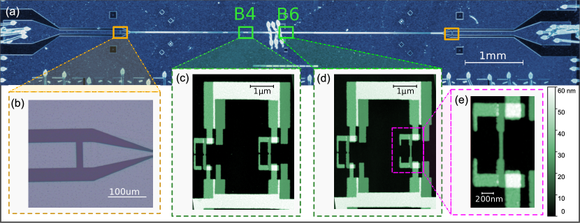
Figure 1: Circuit implementation. (a) Optical microscope image of a $\lambda/2$ CPW resonator (resonator B) intersected and galvanically coupled to a series of eleven flux qubits labelled $B1$ to $B11$. The CPW resonator length is chosen to be 5.73 mm, such that the first resonant mode is at $f_{rB}\simeq 9.8$ GHz. (b) Close up view of the coupling capacitor terminating at both ends the CPW resonator. The value of the capacitance is calculated by an electromagnetic simulator (Sonnet) to be $C_{C}\sim$5.0\text{\,}\mathrm{fF}$$. (c) Colored AFM micrograph of qubit $B4$. The surface area of the unitary junction is $A_{uni}=0.0526\pm$0.0008\text{\,}\mathrm{\SIUnitSymbolMicro m}$^{2}$ and the small junction was chosen to have $\alpha=0.5$. (d) Colored AFM micrograph of qubit $B6$. The surface area of the unitary junction and the ratio $\alpha$ are identical to $B4$. The loop of this qubit includes a thin constriction. (e) Close up view of the 30-nm width constriction of qubit $B6$.

In this work, we present a good improvement in the control and reproducibility of these qubits. We present a systematical study of a large batch of more than twenty devices and demonstrate that it is possible to control their gap energy to within less than $1\text{\,}\mathrm{GHz}$ while obtaining reproducible relaxation times $T_{1}\sim 15-$20\text{\,}\mathrm{\SIUnitSymbolMicro s}$$ and pure dephasing times $T_{2E}^{\phi}\sim 15-$30\text{\,}\mathrm{\SIUnitSymbolMicro s}$$. This reproducibility enabled us to analyze the different factors that impede the coherence times and systematically eliminate them. Our work opens new perspectives for potential applications in the fields of quantum hybrid circuits and quantum computation.

Our method explores the role of the substrate in device variability by employing a standard gate oxide process based on other applications of CMOS device technology [20]. The three samples presented in this work are fabricated on silicon chips and contain a 150-nm thick aluminium coplanar waveguide (CPW) resonator, with two symmetric ports used for microwave transmission measurements (see Figure 1(a)). The CPW resonator A is directly fabricated on a high resistivity ($>$10\text{\,}\mathrm{k\SIUnitSymbolOhm}\text{\,}\mathrm{cm}$$) silicon wafer with native oxide while resonators B and C are fabricated on a 5 nm thermally grown silicon oxide layer. A series of eleven flux qubits is galvanically coupled to each CPW resonator. In the following, the qubits are labelled according to their spatial position on the relevant resonator (e.g. $A1...A11,B1...B11,C1...C11)$.

Our flux qubit design consists of a superconducting loop intersected by four Josephson junctions, one of which is smaller than the others by a factor $\alpha$. This circuit behaves as a two-level system when the flux threading the loop is close to half a flux quantum $\Phi\sim\Phi_{0}/2$ [6, 7]. Each level is characterized by the direction of a macroscopic persistent current $I_{P}$ flowing in the loop of the qubit. The value of the persistent current $I_{P}$ - typically of the order of 200-$300\text{\,}\mathrm{nA}$ - gives rise to a huge magnetic moment ($\sim 500\,\mathrm{GHz/G})$, making the energy of each level very sensitive to external magnetic flux. At $\Phi=\Phi_{0}/2$, the two levels are degenerate, hybridise and give rise to an energy splitting $h\Delta$ called the flux-qubit gap. At this point, the qubit is immune to flux noise at first order and should exhibit a long coherence time.

Figure 1(c) and (d) present Atomic Force Microscope (AFM) images of qubits $B4$ and $B6$. The loop area of qubit $B4$ (resp. $B6$) is $S_{B4}\simeq$13.3\text{\,}\mathrm{\SIUnitSymbolMicro m}$^{2}$ (resp. $S_{B6}\simeq$12.4\text{\,}\mathrm{\SIUnitSymbolMicro m}$^{2}$). The three identical junctions have a Josephson energy $E_{J}/h=$360\text{\,}\mathrm{GHz}$$ and a single electron charging energy $E_{C}/h=$3.68\text{\,}\mathrm{GHz}$$ while the fourth junction is smaller than others by $\alpha$=0.5. In addition, qubit $B6$ contains a 30 nm width constriction over a length of 500 nm (see Figure 1(e)). The qubits are fabricated by e-beam lithography with a tri-layer CSAR-Ge-MAA process (See [21] for more details). The germanium mask is rigid and robust to the oxygen ashing cleaning step. Moreover, it dissipates efficiently the charges during e-beam lithography and thus provides an excellent precision and reproducibility of the junction sizes. The electron-beam lithography is followed by double angle-evaporation of Al–AlOx–Al performed at a well controlled temperature ($-$50\text{\,}\mathrm{\SIUnitSymbolCelsius}$/+$7\text{\,}\mathrm{\SIUnitSymbolCelsius}$)$. The low temperature enables us to reduce the grain size of aluminium, to better control the dimensions and oxidation of our junctions and to fabricate small constrictions with high fidelity.

We first characterize the qubit-resonator system by spectroscopic measurements (see [21] for experimental setup). Figure 2(a-b) shows a continuous wave transmission scan of resonator $B$ taken as a function of the applied magnetic field. This measurement is performed with a vanishing power corresponding to an average of less than one photon in the resonator. We observe an anticrossing each time a qubit and the resonator are resonant. Far from the anticrossings, the resonance corresponding to the first mode of the resonator is $f_{rB}=9.804$ GHz and its quality factor is $Q_{B}=2800$ [21].

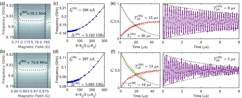
Figure 2: Characterisation of qubit $B4$ (top panels) and $B6$ (bottom panels). (a-b) Transmission spectrum of CPW resonator B versus applied magnetic field showing anticrossing of qubit B4/B6. For each qubit we fit the anticrossing to our qubit-resonator coupling model and extract the value of the coupling constant $g$ of the qubit with the resonator. (c-d) Measured qubit frequency (blue dots) and fit (black dashed curve) yielding the qubit parameters $\Delta$ and $I_{p}$. (e-f) (left panel) Qubit energy relaxation and spin echo measurements. The excited state probability $P_{e}$ is plotted as a function of the delay between the $\pi$ pulse and the readout pulse (green dots) or between the two $\pi/2$ pulses of the echo sequence (red dots). The black dashed line is an exponential fit to the energy relaxation (spin-echo) data. (Right panels) Measured Ramsey fringes (purple solid line) with fit to its exponentially decaying envelope.

The frequency dependence of qubit $B4$ and $B6$ on $\Phi$ is shown in Figure 2(c-d), respectively. The transition frequency of each qubit follows $f_{01}=\sqrt{\Delta^{2}+\varepsilon^{2}}$ with $\varepsilon=2I_{P}\left(\Phi-\Phi_{0}/2\right)/h$, yielding $\Delta^{(B4)}=$5.182\text{\,}\mathrm{GHz}$$ and $I_{P}^{(B4)}=$298\text{\,}\mathrm{nA}$$ (resp. $\Delta^{(B6)}=$5.085\text{\,}\mathrm{GHz}$$, $I_{P}^{(B6)}=$297\text{\,}\mathrm{nA}$$). Since both qubits were designed to have the same parameters, this demonstrates excellent reproducibility of our e-beam lithography and oxidation parameters. Taking into account the contribution of geometric capacitance between neighboring islands allows us to fit the parameters of the flux-qubits in good agreement with the measured values of $\alpha$ and $E_{J}$ extracted from Ambegaokar-Baratoff formula (see [21]). We now turn to the coherence times at the so-called optimal point where the qubit frequency $f_{01}=\Delta$ is insensitive to first order to flux-noise [13, 14]. Energy relaxation decay is shown in Figure 2(e) and f to be exponential for both qubits, with $T_{1}=$20\text{\,}\mathrm{\SIUnitSymbolMicro s}$$ for $B4$ and $19\text{\,}\mathrm{\SIUnitSymbolMicro s}$ for $B6$. Ramsey fringes show an exponential decay for $B4$ with $T_{2R}=$9\text{\,}\mathrm{\SIUnitSymbolMicro s}$$, for $B6$ with $T_{2R}=$5\text{\,}\mathrm{\SIUnitSymbolMicro s}$$. Spin-echo decays exponentially with identical dephasing times $T_{2E}=$13\text{\,}\mathrm{\SIUnitSymbolMicro s}$$. Apparently, the presence of the constriction in qubit $B6$ does not seem to influence the coherence time of the qubit. This property is particularly exciting if one wishes to coherently couple a single spin to this circuit [12].

We repeat this procedure for the qubits of our three samples. Each qubit is thus characterized by its spectroscopic parameters $\Delta$ and $I_{P}$, extracted from the dependence of its transition frequency on the applied flux. In Figure 3(a), we represent a graph showing the gaps $\Delta$ of the different qubits versus their persistent currents $I_{P}$. In order to optimize our qubit design, we varied the size of the unitary junctions of samples A, B and C while keeping an approximately constant critical current density of $\sim$13.5\text{\,}\mathrm{\SIUnitSymbolMicro A}\text{\,}{\mathrm{\SIUnitSymbolMicro m}}^{-2}$$. Within each sample, the qubit parameters $\left(E_{J},E_{C},\alpha\right)$ were designed to be identical and thus the qubits should be clustered within a well defined region. The extent of this region indicates the level of reproducibility of our fabrication process. A slight improvement in the data spread is observed for Sample B and C in comparison to sample A. Quantitatively speaking, the gap average values are $6.9\pm 1$GHz, $5.1\pm 0.7$ GHz and $6.6\pm 0.6$ GHz for samples A, B and C respectively. A principal component analysis (PCA) is performed on the covariance matrix of the $(\Delta,I_{P})$ data-points in order to define regions with high probability to find a qubit. For each sample, a dashed line is represented and corresponds to the result of qubit numerical diagonalizations (see [21]) while varying the parameter $\alpha$ by $\pm 5\%$ around their respective average value $\left(\left\langle E_{J}\right\rangle_{A/B/C},\left\langle E_{c}\right\rangle_{A/B/C},\left\langle\alpha\right\rangle_{A/B/C}\right)$. For the three samples, the principal axis and the numerical diagonalizations are well aligned indicating that the main origin of disorder is indeed uncontrolled variations of the value of the parameter $\alpha$. The variation of the critical current density of the junctions due to different oxidation of samples A, B and C ($\pm 5\%$) leads to an additional uncertainty of $\pm$150\text{\,}\mathrm{MHz}$$ in the control of the desired qubit gap.

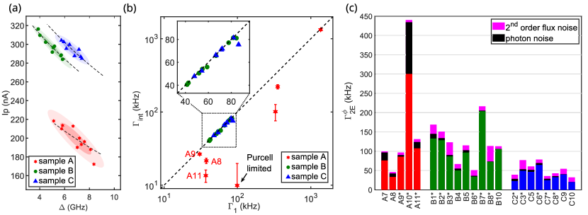
Figure 3: Reproducibility and control. (a) Persistent current $I_{P}$ versus gap $\Delta$ of the qubits of sample A (native oxide, red stars), sample B ($5\text{\,}\mathrm{nm}$ grown silicon oxide layer, green dots) and sample C ($5\text{\,}\mathrm{nm}$ grown silicon oxide layer, blue triangles). The colored regions are obtained by assuming a normal distribution along axes defined by principal component analysis (PCA). The probability to find a qubit within the dark (resp. light) colored area is 50% (resp. 90%). The dashed black lines are obtained by numerical simulations of the flux qubits (see [21]) at their average value $\left(\left\langle E_{J}\right\rangle_{A/B/C},\left\langle E_{c}\right\rangle_{A/B/C},\left\langle\alpha\right\rangle_{A/B/C}\right)$ while varying the parameter $\alpha$ by $\pm 5\%$. (b) The estimated intrinsic relaxation rates $\Gamma_{int}=\Gamma_{1}-\Gamma_{P}$ versus measured relaxation rates $\Gamma_{1}$ for qubits of sample A (red stars), B (green dots) and C (blue triangles). The error bars stem from calibration uncertainties of $\pm$1\text{\,}\mathrm{dB}$$ of the incoming power at the resonator input. (c) Stacked bar chart showing the pure dephasing rates $\Gamma_{2E}^{\phi}$ at optimal points of the measured qubits of sample A (red), B (green) and C (blue). The black color corresponds to the calculated decoherence rate due to photon noise in the resonator. The pink color corresponds to calculated decoherence rate due to second order flux noise. The black stars indicate the presence of a 30-nm width constriction in the loop of the qubit. The presence of a constriction does not seem to affect significantly the relaxation or the dephasing of the qubits.

In Figure 3(b), we represent the spread of the relaxation rates $\Gamma_{1}$ of the different qubits. Qubit $A9$ exhibits the longest relaxation time with $T_{1}=$32\text{\,}\mathrm{\SIUnitSymbolMicro s}$$. Several mechanisms contribute to relaxation of qubits; among them, spontaneous emission by the qubit to the resonator (the so-called Purcell effect [22]). The Purcell rate $\Gamma_{P}$ can be quantitatively determined by measuring the qubit Rabi frequency $\Omega_{R}$ for a given microwave power $P_{in}$ at the resonator input. For a qubit coupled symmetrically to the input and output lines, a simple expression for $\Gamma_{P}$ was obtained in Ref. [17]. We thus calculated $\Gamma_{P}$ for each qubit and represented the intrinsic relaxation rates of the qubits defined as $\Gamma_{int}=\Gamma_{1}-\Gamma_{P}$. The average values of the intrinsic relaxation rates are $260\pm 440$ kHz, $61\pm 15$ kHz and $68\pm 11$ kHz for samples A, B and C, respectively. These average numbers are comparable to those obtained in Ref. [19] for C-shunted flux qubits. Relaxation due to $1/f^{\gamma}$-flux noise can be safely neglected for qubits in our frequency range [19]. The spread of the relaxation rates in sample B and C is remarkable compared to sample A and more generally to the state of the art [18, 17]. We thus come to the conclusion that better qubit reproducibility in terms of relaxation rates is obtained on samples with a thermally grown 5 nm width silicon oxide layer. It is yet important to stress that the best relaxation rates ($\sim$25\text{\,}\mathrm{kHz}$$) were obtained on intrinsic silicon (e.g. A11, A8). These findings are consistent with previous studies comparing loss tangents for silicon oxide and silicon at low temperatures [23, 24, 25]. Yet, the high variability of the devices on native oxide points towards an extreme sensitivity of the dielectric losses to the nanoscale variations in the stoichiometry and thickness of the oxide.

In the rest of the paper, we will focus on the origin of the dephasing rates of the qubits. Indeed, the noticeable reproducibility of the qubits enables us to analyze the different noise sources that influence the coherence times and systematically eliminate possible noise factors. We begin this analysis away from the optimal point, where the flux qubit decoherence is dominated by flux noise. The power spectrum of flux noise has a 1/f shape $S_{\varPhi}\left[f\right]=A_{\varPhi}^{2}/f$ [13, 16, 17, 18]. Thus, measuring the flux qubit decoherence versus $\varepsilon$ gives us directly access to the flux noise amplitude $A_{\varPhi}$ [26, 27]. Interestingly, we obtain almost the same flux noise amplitude $A_{\varPhi}=1.2\pm 0.2\>\mu\varPhi_{0}$ for all the qubits whether on sample A, B or C including those with constrictions or not (see [21]).

In Figure 3(c), we show the pure echo dephasing rate $\Gamma_{2E}^{\phi}=\Gamma_{2E}-\Gamma_{1}/2$ at the optimal point for the different qubits. At this point, the qubits are protected against flux noise at first order. Yet, second order effects may still impact the dephasing rates. To account for these effects, we performed a numerical Monte Carlo simulation detailed in [21]. At the optimal point, a simple formula is obtained:

$$\Gamma_{2E}^{opti}\simeq 56\frac{(I_{p}A_{\varPhi}/h)^{2}}{\Delta}$$

The results of our analysis show that second order flux noise can only explain partially the observed dephasing at the optimal point. Other well-known mechanisms of dephasing are related to photon noise in the resonator [13, 19] and charge noise [17]. As shown in Figure 3(c), photon noise has some impact on several qubits whose resonance happens to be close to the one of the resonator. The sensitivity of flux qubits to charge-noise is highly dependent on the ratio between the Josephson energy $E_{J}$ and the charging energy $E_{C}$. We thus calculated the maximum amplitude of the charge modulation for each qubit (See [21]). In average, the charge modulation is equal to 100 kHz, 5 kHz and 1 kHz for samples A, B and C respectively. Clearly, this is more than one order of magnitude smaller than the measured pure dephasing rate for sample B and C and cannot explain the data. Thus, another mechanism is necessary to explain at least qualitatively the remaining dephasing rate of these qubits. Critical current fluctuations are for instance a possible channel of dephasing in our system. These fluctuations are due to charges localised in the barrier of the Josephson junctions. They also produce a 1/f shape spectral density [28, 29]. Assuming that the remaining dephasing rate of sample C is fully due to this microscopic source of noise, we get $S_{I_{0}}[$1\text{\,}\mathrm{Hz}$]\simeq\left($0.5\text{\,}\mathrm{pA}$\right)^{2}${\mathrm{\SIUnitSymbolMicro m}}^{-2}$$, which seems compatible with previously reported values in the literature.

In conclusion, we have shown that flux qubits can be fabricated in a reproducible way both in terms of gap transition energy and in terms of decoherence rates. Reproducible relaxation times have been measured with $T_{1}\sim 15-$20\text{\,}\mathrm{\SIUnitSymbolMicro s}$$ for samples fabricated on a thermally grown 5-nm $\mathrm{SiO_{2}}$ layer. These numbers are comparable to those observed in Ref. [19] for C-shunted flux qubits. The major advantages of our design are its large anharmonicity ($f_{12}\sim$30\text{\,}\mathrm{GHz}$$) and high persistent current ($I_{p}\sim$300\text{\,}\mathrm{nA}$$). This makes flux qubits ideal candidates for magnetic coupling to spins such as NV centers [10, 12] or other impurities in silicon [30]. In all the samples, the amplitude of flux noise was low and reproducible $A_{\phi}=1.2\pm 0.2\>\mu\varPhi_{0}/\sqrt{\mathrm{Hz}}$. At the optimal point, long and reproducible pure dephasing times were measured with $T_{2E}^{\phi}=15-$30\text{\,}\mathrm{\SIUnitSymbolMicro s}$$. At this level, the pure dephasing times are most likely limited by critical current fluctuations of the small junction of the qubits. Our results prove that flux qubits can reliably reach long coherence times and open interesting new perspectives for both hybrid quantum circuits and scalable quantum processing.

Supplementary Materials

I Experimental Setup

Experiments are performed at a temperature of $14\text{\,}\mathrm{mK}$ in a Cryoconcept dilution refrigerator, model Hexadry 200 with low mechanical vibrations. Supplementary Figure 1 shows a detailed schematic of the experimental setup. The samples are glued on a microwave printed circuit board made out of TMM10 ceramics, then enclosed in a copper box with low mode volume which is itself embedded into a superconducting coil that is used to provide magnetic flux biases to the qubits. To reduce low frequency magnetic noise, the coil is surrounded by a superconducting enclosure (Copper plated by SnPb 60/40 $15\text{\,}\mathrm{\SIUnitSymbolMicro m}$) and magnetically shielded with a high permeability metal box (CryoPhy from Meca Magnetic). The apertures of the box are tightly closed using Eccosorb AN-72, in order to protect the sample from electromagnetic radiation that could generate quasiparticles.

The coil is powered by a BILT BE-2102 voltage source filtered by a custom designed ultra-stable voltage to current converter. The microwaves are generated by Keysight PSG E8257D analog microwave synthesizers. The pulses are modulated at an intermediate frequency of 10-200 MHz by a Quantum Machines OPX system connected to MITEQ IRM0618/IRM0408 mixers. Voltage controlled attenuators (Pulsar AAR-29-479) are used to adjust the pulse amplitude over a wide range (0.5-64 dB). The input line is attenuated at 4K stage (XMA -20 dB) and at the mixing chamber stage (XMA -40 dB) to minimize thermal noise and filtered with an homemade impedance-matched copper powder filter (-10 dB @ 10 GHz). In addition, the pulses are shaped with smooth rise and fall ($\sim 20$ ns) in order to reduce the population of microwave photons in the resonator during coherent state evolution of the qubit.

Qubit state measurement is done using dispersive readout, by measuring the transmission of microwave pulses through the resonator, using a custom built setup. The readout output line is filtered by two shielded double circulators (LNF-CICIC8_12A) and a $8-$12\text{\,}\mathrm{GHz}$$ band pass filter from Micro-Tronics, model BPC50406. The readout output signal is amplified using a low-noise cryogenic HEMT amplifier (LNF-LNC1_12A) and a room temperature amplifier (LNF-LNR1_15A). After demodulation, the quadratures of the readout output pulse are sampled and averaged using the IQ inputs of the OPX system. At this point, we perform a principal axis transformation on the data points by diagonalizing their covariance matrix. Using this transformation, we extract the largest principal component of the measured $(I,Q)$ points and obtain the state of the qubit.

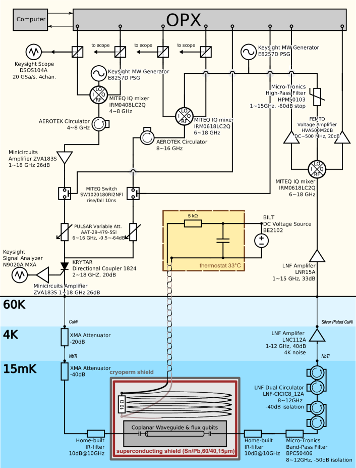
Figure 4: Experimental Setup.

II Flux Qubit Model

The flux qubit consists of a superconducting loop intersected by four Josephson junctions among which one is smaller than others by a factor $\alpha$. 5 shows a schematic drawing of a flux qubit. Each Josephson junction is characterized by its Josephson energy $E_{J}$ and its bare capacitance $C_{J}$. The junctions divide the loop into four superconducting islands. The island $I_{1}$ is galvanically connected to the coplanar waveguide resonator. Each island is capacitively coupled to its surrounding by geometric capacitances denoted as $C_{ij}$ where $\left(i,j\right)\in\left(0,1,..,4\right)$, the index 0 representing the ground.

Figure 5: Equivalent circuit diagram of a flux qubit. The Josephson junctions are defined by their Josephson energy $E_{J}$ and their bare capacitance $C_{J}$. The island $I_{1}$ is galvanically connected to the coplanar waveguide resonator. Each island is capacitively coupled to its surrounding by geometric capacitances denoted as $C_{ij}$ where $\left(i,j\right)\in\left(0,1,..,4\right)$, the index 0 representing the ground.

II.1 Potential Energy

The potential energy of the circuit shown in 5 corresponds to the inductive energy of the junctions and can be written as

$$U=-\sum_{j=1}^{3}E_{J}\cos\varphi_{j,j+1}-\alpha E_{J}\cos\varphi_{41}$$ (1)

where $\varphi_{j,k}$ denotes the phase difference $\varphi_{k}-\varphi_{j}$ between islands $j$ and $k$.

Faraday law implies that

$$\varphi_{41}=2\pi\frac{\Phi}{\Phi_{0}}-\sum_{j=1}^{3}\varphi_{j,j+1}$$ (2)

where $\Phi$ is the flux threading the qubit loop and $\Phi_{0}=h/2e$.

When $\Phi=\Phi_{0}/2$, the potential energy has two degenerated minima. The positions of these minima are given by solving the partial differential equations $\partial_{\varphi_{i}}U=0$. The two solutions verify the simple equation $\sin\varphi^{*}=\alpha\sin 3\varphi^{*}$ and correspond to two opposite persistent currents given by

$$I_{p}=\pm I_{0}\sqrt{\frac{3}{4}-\frac{1}{4\alpha}}$$ (3)

where $I_{0}$ is the critical current of the Josephson junctions.

II.2 Kinetic Energy

The kinetic energy $K$ of the system is the sum of the capacitive energies of the circuit

$$K=\frac{1}{2}\sum_{i\neq j}C_{ij}\left(V_{j}-V_{i}\right)^{2}+\frac{1}{2}C_{J}\left(\left(V_{1}-V_{2}\right)^{2}+\left(V_{2}-V_{3}\right)^{2}+\left(V_{3}-V_{4}\right)^{2}+\alpha\left(V_{4}-V_{1}\right)^{2}\right)$$ (4)

It is a quadratic form of the island voltages $V_{i}$ and can thus be written as

$$K=\frac{1}{2}\mathbf{V}^{T}\mathbf{C}\mathbf{V}$$ (5)

where $\mathbf{V^{T}}=\left(\begin{array}[]{cccc}V_{1}&,V_{2}&,V_{3},&V_{4}\end{array}\right)$ and $\mathbf{C}$ is a $4\times 4$ matrix which we will refer in the following as the capacitance matrix. The matrix $\mathbf{C}$ can be written as the sum of the Josephson capacitance matrix $\mathbf{C_{J}}$ and the geometric capacitance matrix $\mathbf{C_{geom}}$:

$$\mathbf{C}=\mathbf{C_{J}}+\mathbf{C_{geom}}$$ (6)

where

$$\mathbf{C_{J}}=C_{J}\left(\begin{array}[]{cccc}1+\alpha&-1&0&-\alpha\\ -1&2&-1&0\\ 0&-1&2&-1\\ -\alpha&0&-1&1+\alpha\end{array}\right)$$ (7)

and

$$\mathbf{C_{geom}}=\left(\begin{array}[]{cccc}C_{10}+\sum_{j\neq 1}C_{1j}&-C_{12}&-C_{13}&-C_{14}\\ -C_{21}&C_{20}+\sum_{j\neq 2}C_{2j}&-C_{23}&-C_{24}\\ -C_{31}&-C_{32}&C_{30}+\sum_{j\neq 3}C_{3j}&-C_{34}\\ -C_{41}&-C_{42}&-C_{43}&C_{40}+\sum_{j\neq 4}C_{4j}\end{array}\right)$$ (8)

We determined the capacitance matrix $\mathbf{C_{geom}}$ using an electrostatic simulator (COMSOL) and according to the prescriptions detailled herein below.

II.3 Numerical Estimation of the Geometrical Capacitance

Numerical Estimation of the geometrical capacitance using finite element solvers is difficult due to the different length scales involved. The qubits have typically micron size dimensions while the oxide thickness is rather of the order of 1 nm. As a consequence, a fine meshing is difficult to establish. In this section, we will present an approach which provides satisfactory results.

II.3.1 Coarse estimation

We first performed a coarse simulation using the electrostatic module of COMSOL. To perform this simulation, we assumed Neumann boundary conditions (zero charge) on a box of $30\,$\mathrm{\SIUnitSymbolMicro m}$$ surrounding the qubit (see 6). The oxide of the Josephson junctions was replaced by a hollow box of thickness $l=$20\text{\,}\mathrm{n}\mathrm{m}$$. We defined a minimum meshing size of $4\text{\,}\mathrm{n}\mathrm{m}$. For these mesh parameters, the far field components are accurately calculated. Isolated islands not participating in the flux qubit loop were set to charge conservation $Q=0$ terminal settings.

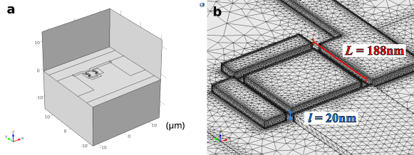
Figure 6: Coarse Simulation using the electrostatic module of COMSOL. a, The precise design of the qubit is imported to the simulator and put into a cubic box of $30\,$\mathrm{\SIUnitSymbolMicro m}$$ edge, where zero charge boundary condition is imposed. b, Close-up view of the meshing around one of the junction. The junction is modelized by conducting planes separated by 20 nm distance in order to keep a minimal meshing size of 4 nm.

We applied sequentially a voltage on each island in order to construct the capacitance matrix $\mathbf{C_{coarse}}$. For instance, the coarse capacitance matrix of qubit B4 is

$$\mathbf{C_{coarse}}=\left(\begin{array}[]{cccc}3.752&-0.181&-0.524&-0.137\\ -0.181&0.350&-0.148&-0.002\\ -0.524&-0.148&1.044&-0.140\\ -0.137&-0.002&-0.140&0.300\end{array}\right)\qquad\mathrm{fF}$$

II.3.2 Estimating the capacitance between edges

In order to obtain more precise results, the capacitance between adjacent edges needs to be corrected. In 7 , we represent a close-up view of a typical Josephson junction obtained by Dolan technique, where we show the four edge capacitances we need to consider. The two capacitances $C_{\text{edge}}^{\text{Si}}$ are dominant due to the high permittivity constant of Si and thus $C_{\text{edge}}^{\text{air}}$ can be neglected in a first approximation.

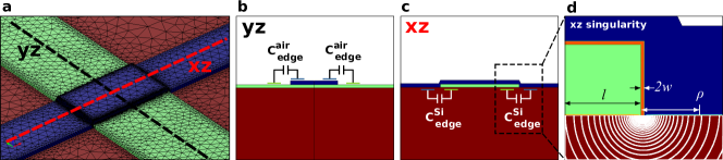
Figure 7: Edge capacitances. a, 3D representation of a Josephson junction obtained by double angle evaporation. b, View cut of the junction in the yz plane showing the $C_{edge}^{air}$ edge capacitances. c, View cut of the junction in the xz plane showing the $C_{edge}^{Si}$ edge capacitances. d, Close up view of the edge showing the electric field lines giving rise to the edge capacitances. We show the edge length $l$, the distance to the singularity $\rho$, and the oxide thickness $2w$.

The capacitance between adjacent edges of length $l=20$ nm and width $L$ separated by an oxide layer in the region$\left|\rho\right|<w$ (See 7d) can be calculated analytically. By using Gauss theorem, we have

$$L\int_{w}^{l}\frac{V}{\pi\rho}d\rho=\frac{Q}{\epsilon_{0}\epsilon_{r}}$$ (9)

where $V$ is the voltage potential in the silicon substrate at a distance $\rho$ from the junction singularity, $\epsilon_{0}\epsilon_{r}$ is the dielectric permittivity of silicon and $Q$ the charge accumulated on the surface of the metallic island. Thus, the capacitance is given by

$$C_{edge}^{Si}=L\frac{\epsilon_{0}\epsilon_{r}}{\pi}\ln\frac{l}{w}$$ (10)

For instance, the edge capacitance matrix of qubit B4 is

$$\mathbf{C_{edge}}=\left(\begin{array}[]{cccc}0.069&-0.042&0&-0.027\\ -0.042&0.084&-0.042&0\\ 0&-0.042&0.084&-0.042\\ -0.027&0&-0.042&0.069\end{array}\right)\qquad\mathrm{fF}$$

II.3.3 Numerical results

Following the procedure described herein above, the capacitances matrix of qubit B4 is calculated and given here as an example:

$$\mathbf{C_{J}} =\left(\begin{array}[]{cccc}7.898&-5.265&0&-2.633\\ -5.265&10.531&-5.265&0\\ 0&-5.265&10.531&-5.265\\ -2.633&0&-5.265&7.898\end{array}\right)\qquad\mathrm{fF}$$

$$\mathbf{\mathbf{C_{geom}}} =\mathbf{C_{coarse}}+\mathbf{C_{edge}}=\left(\begin{array}[]{cccc}3.821&-0.223&-0.524&-0.164\\ -0.223&0.434&-0.190&-0.002\\ -0.524&-0.190&1.128&-0.182\\ -0.164&-0.002&-0.182&0.370\end{array}\right)\qquad\mathrm{fF}$$

This matrix is then inserted in the Lagrangian of the qubit as we will see herein below.

II.4 Legendre Transformation and Hamiltonian

The Lagrangian of the system is $\mathcal{L}=K-U$. The conjugate momenta of our system are given by

$$n_{j}\equiv\frac{1}{\hbar}\frac{\partial\mathcal{L}}{\partial\dot{\varphi}_{j,j+1}}$$ (11)

Since $\frac{\varPhi_{0}}{2\pi}\dot{\varphi}_{j,j+1}=V_{j+1}-V_{j}$, it is neccessary to express the kinetic energy terms in a new basis. Since island $I_{1}$ is galvanically connected to the central conductor of the CPW, we can safely assume that $V_{1}=0\,\mathrm{V}$, which simplifies considerably the transformation:

$$V_{1} =0$$

$$V_{2} =\cancelto{0}{V_{1}}+V_{12}$$

$$V_{3} =\cancelto{0}{V_{1}}+V_{12}+V_{23}$$

$$V_{4} =\cancelto{0}{V_{1}}+V_{12}+V_{23}+V_{34}$$

where $V_{ij}=V_{j}-V_{i}$. The passage matrix $P$ between these two bases can be thus written as

$$\mathbf{P}=\left(\begin{array}[]{ccc}0&0&0\\ 1&0&0\\ 1&1&0\\ 1&1&1\end{array}\right)$$ (12)

The Hamiltonian $\mathcal{H}$ is then obtained by the Legendre transformation $\mathcal{\mathcal{H}}=\hbar\sum_{j=1}^{3}\dot{\varphi}_{j,j+1}n_{j}-\mathcal{L}$ and thus writes

$$\mathcal{H}=\frac{\left(2e\right)^{2}}{2}n^{T}\left(\mathbf{P}^{T}\mathbf{C}\mathbf{P}\right)^{-1}n+U$$ (13)

This Hamiltonian can be expressed in the so-called charge basis $\left|n_{1},n_{2},n_{3}\right\rangle,\forall n_{1},n_{2},n_{3}\in\mathbb{Z}^{3}$, noting that

$$\cos\varphi_{j,j+1}\left|n_{1},n_{2},n_{3}\right\rangle=\frac{1}{2}\left(\left|n_{1}+\delta_{j1},n_{2}+\delta_{j2},n_{3}+\delta_{j3}\right\rangle+\left|n_{1}-\delta_{j1},n_{2}-\delta_{j2},n_{3}-\delta_{j3}\right\rangle\right)$$ (14)

In this basis the operator $\frac{\left(2e\right)^{2}}{2}n^{T}\left(\mathbf{P}^{T}\mathbf{C}\mathbf{P}\right)^{-1}n$ is diagonal while the operator $U$ is sparse. The precision of the eigenvalues and eigenstates depends on the truncation of the $n_{j}$ bases. With $n_{k}=-10...10$, we would need $21^{3}$ coefficients just to describe the wavefunction and another $\left(21^{3}\right)^{2}$ to describe the Hamiltonian matrix. Thanks to the the sparsity of the Hamiltonian operator, the number of nonzero entries in this matrix is only $21^{3}\times\left(1+4\times 2\right)$. This resolution in charge space is computationally feasible both to store and diagonalize matrices efficiently. For reaching the necessary precision to resolve charge modulation, we used $n_{k}=-14...14$ and verified carefully the numerical convergence of the calculation.

II.5 Pseudo-Hamiltonian

Following the full diagonalization of the Hamiltonian, we obtain the spectrum of the flux qubit by subtracting the energy of the first excited state $\left|1\right\rangle$ from the energy of the ground state $\left|0\right\rangle$. It can be shown that close to $\Phi=\Phi_{0}/2$, the system behaves as a two level system and the spectrum can be fully described by two parameters:

• The value of the persistent current $I_{p}$, already discussed previously.

• The so-called flux qubit gap, denoted as $\Delta$, which corresponds to the tunneling term between the two potential minima.

The value of the gap can be directly measured by the transition energy at half a flux quantum $\Phi=\Phi_{0}/2$. This point is known as the optimal point of the flux qubit due to its immunity at first order in flux noise, as will be explained in later sections. In the vicinity of the optimal point, the Hamiltonian of the system can be written using perturbation theory as

$$\begin{array}[]{c}\mathcal{H}=\mathcal{H}_{0}-\alpha E_{J}\partial_{\Phi}\left(\text{cos}(2\pi\frac{\Phi}{\Phi_{0}}-\sum_{j=1}^{3}\varphi_{j,j+1})\right)_{\Phi=\Phi_{0}/2}\cdot\left(\Phi-\frac{\Phi_{0}}{2}\right)\\ =\mathcal{H}_{0}+\frac{1}{\varphi_{0}}\left[\underbrace{\alpha E_{J}\text{sin}\left(\varphi_{41}\right)}_{\hat{I}\cdot\varphi_{0}}\left(\Phi-\frac{\Phi_{0}}{2}\right)\right]=\mathcal{H}_{0}+\hat{I}\cdot\left(\Phi-\frac{\Phi_{0}}{2}\right)\end{array}$$ (15)

When the current operator is projected on the eigenstates $\left|0\right\rangle,\left|1\right\rangle$ of $\mathcal{H}_{0}$ we get

$$\begin{array}[]{ccc}\left\langle 0\right|\hat{I}\left|0\right\rangle=0&,&\left\langle 0\right|\hat{I}\left|1\right\rangle=I_{p}\\ \left\langle 1\right|\hat{I}\left|0\right\rangle=I_{p}&,&\left\langle 1\right|\hat{I}\left|1\right\rangle=0\end{array}$$ (16)

Therefore, the Hamiltonian of the system can be written in this basis as

$$\mathcal{H}_{\text{eff}}=\frac{h}{2}\left[\Delta\sigma_{z}+\varepsilon\sigma_{x}\right]$$ (17)

where $\varepsilon=\frac{2I_{p}}{h}\left(\Phi-\frac{\Phi_{0}}{2}\right)$.

The frequency of the qubit is thus given by

$$\frac{\omega_{01}}{2\pi}=\sqrt{\Delta^{2}+\varepsilon^{2}}$$ (18)

II.6 Doublet at optimal point

Some of the measured qubits exhibit a doublet line shape at optimal point. This lineshape is manifested as a beating of the Ramsey oscillations as shown in 8. For qubit $B5$, the frequency of this beating is $340\>\mathrm{kHz}$, almost two orders of magnitude larger than the charge modulation $\delta\Delta^{n_{g}}=4.3\>\mathrm{kHz}$ and thus cannot be attributed to slow fluctuations of the electron number parity on one of the qubit’s islands [17, 31]. An alternative explanation for the origin of this doublet is related to trapping and un-trapping of a single quasiparticle in the $\alpha$ junction.

By simple arguments, we can give a rough estimate for this effect. The area of the $\alpha$ junction of qubit $B5$ is $A_{\alpha}=0.0257\>\mathrm{\mu m^{2}}$while the Fermi wavelength of electrons in Aluminium is $\lambda_{F}=0.36\>\mathrm{nm}.$ Thus, the number of channels in such a junction is large and can be estimated as $A_{\alpha}/\lambda_{F}^{2}\sim 2\times 10^{5}$. Assuming that all channels have the same transmission $\tau$, we can estimate the change of the Josephson energy of the $\alpha$ junction to be around $1\>\mathrm{MHz}.$ We then calculate numerically the variation $\delta\Delta^{\text{trapping}}$ of the qubit gap and obtain 300 kHz , which is close to the observed value of the doublet. We thus come to the conclusion that these doublets are most likely due to the trapping and un-trapping of a quasiparticle in the $\alpha$ junction.

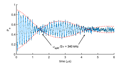
Figure 8: Ramsey measurement of qubit B5 showing beating.

III Estimating dephasing due to flux noise

III.1 Pure Dephasing of a flux qubit

In an ideal system, the decoherence rate $\Gamma_{2}$ is limited by the energy relaxation rate of the qubit and is given by $\Gamma_{2}=\Gamma_{1}/2$ . In practice, the decoherence rate of a qubit may be much larger than this theoretical limit. There are several known sources of dephasing which are responsible for this. Among them, flux noise, charge noise and photon noise in the resonator. The pure dephasing rate of the flux qubit can be estimated by the so-called Ramsey sequence, where two identical $\pi/2$ pulses are played consecutively with a time delay $t$. It is possible to dynamically decouple the noise responsible for this dephasing by playing a more complex set of pulses. The most popular technique to achieve this is called Hahn Echo technique and consists of playing a $\pi$-pulse in between the two $\pi/2$ pulses. This $\pi$ pulse inverses the time evolution and therefore cancels the contribution to dephasing of low frequency noise.

In the Ramsey sequence, the first $\pi/2$-pulse raises the qubit initially in its ground state into a coherent superposition of $\left|\Psi(0)\right\rangle=\left(\left|0\right\rangle+\left|1\right\rangle\right)/\sqrt{2}$ . During time $t$, the qubit performs a free evolution and accumulates phase $\varphi(t)$ and becomes $\left|\Psi(t)\right\rangle=\left(\left|0\right\rangle+e^{i\varphi(t)}\left|1\right\rangle\right)/\sqrt{2}$. The phase $\varphi(t)$ consists of two parts $\varphi(t)=\omega_{01}t+\delta(t)$, where $\delta(t)$ is the phase due to the small fluctuations $\delta\lambda(t)$ which slightly modify the qubit Hamiltonian. At first order, $\delta(t)$ is given by $\delta(t)=\frac{\partial\omega_{01}}{\partial\lambda}\int_{0}^{t}\delta\lambda(t^{\prime})dt^{\prime}$. The decoherence rate of the system corresponds to the decay of the expectation value $\left\langle\sigma_{x}(t)\right\rangle$ and is given by

$$\left\langle\sigma_{x}(t)\right\rangle=1/2\,\left\langle e^{i\varphi(t)}+e^{-i\varphi(t)}\right\rangle$$

When repeating the measurements, the value of $\left\langle\sigma_{x}(t)\right\rangle$ is changed due to the varying environmental noise $\delta(t)$. Therefore, one should average the value of $e^{\pm i\delta(t)}$ in order to determine the influence of this noise. If the fluctuations $\delta\lambda(t^{\prime})$ are small enough, they can be considered as a random variable with Gaussian distribution [26]. Thus,

$$f_{R}(t)=\left\langle e^{\pm i\delta(t)}\right\rangle\approx\left\langle 1\pm\cancel{i\delta}-\delta^{2}/2\right\rangle=e^{-1/2\left\langle\delta^{2}\right\rangle}$$

The expectation value of $\left\langle\sigma_{x}(t)\right\rangle$ will therefore decay according to

$$f_{R}(t) =e^{-1/2\left(\frac{\partial\omega_{01}}{\partial\lambda}\right)^{2}\left\langle\left(\int_{0}^{t}\delta\lambda(t^{\prime})dt\right)^{2}\right\rangle}$$ (19)

$$\text{= exp}\left(-\frac{t^{2}}{2}\left(\frac{\partial\omega_{01}}{\partial\lambda}\right)^{2}\stackrel{{\scriptstyle[}}{{-}}\infty]{\infty}{\int}d\omega\,S_{\lambda}(\omega)\,\text{sinc}^{2}(\frac{\omega t}{2})\right)$$ (20)

In a Hahn echo sequence, the first $\pi/2$-pulse puts the state of the qubit in a coherent superposition state $\left|\Psi(0)\right\rangle=\left(\left|0\right\rangle+\left|1\right\rangle\right)/\sqrt{2}$ . During the time $t_{1}$, the qubit performs a free evolution and accumulates phase $\varphi_{1}(t_{1})=\omega_{01}t_{1}+\delta_{1}(t_{1})$. The $\pi$ - pulse flips the time evolution of the qubit such that during the time $t_{2}$ it acquires an opposite phase $\varphi_{2}(t_{2})=-\omega_{01}t_{2}-\delta_{2}(t_{2})$. The phase accumulated by $\omega_{01}t_{1}$ and $\omega_{01}t_{2}$ is canceled when $t_{1}=t_{2}=t/2$ and the decoherence rate of the qubit - corresponding to the decay $f_{E}(t)=\left\langle\sigma_{x}(t)\right\rangle$ - is given by

$$f_{E}(t)=\left\langle e^{\pm i(\delta_{1}-\delta_{2})}\right\rangle\approx\text{exp}\left(-1/2\left\langle\delta_{1}^{2}+\delta_{2}^{2}-\delta_{1}\delta_{2}-\delta_{2}\delta_{1}\right\rangle\right)$$

The expectation value of $\left\langle\sigma_{x}(t)\right\rangle$ will therefore decay according to

$$f_{E}(t)=\text{exp}\left(-\frac{t^{2}}{2}\left(\frac{\partial\omega_{01}}{\partial\lambda}\right)^{2}\stackrel{{\scriptstyle[}}{{-}}\infty]{\infty}{\int}d\omega\,S_{\lambda}(\omega)\,\text{sin}^{2}(\frac{\omega t}{4})\,\text{sinc}^{2}(\frac{\omega t}{4})\right)$$ (21)

III.2 Dephasing away from the optimal point

Away from the optimal point , the high magnetic moment of the circuit ($\sim 500\,\mathrm{GHz/G})$ make its frequency very sensitive to flux

$$\partial_{\Phi}\omega_{01}=\frac{\partial\varepsilon}{\partial\varPhi}.\frac{\partial\omega_{01}}{\partial\varepsilon}=\left(\frac{2I_{p}}{\hslash}\right)^{2}\frac{\left(\Phi-\Phi_{0}/2\right)}{\omega_{01}}$$

The power spectrum of flux noise has a 1/f shape $S_{\varPhi}\left[\omega\right]=A_{\varPhi}^{2}/\omega$. For the Echo sequence, one can calculate exactly the integral given in 21 without any additionnal assumption or approximation and one obtains [26]

$$\Gamma_{2E}^{\varphi}\left(\Phi\right)=\left(\frac{2I_{p}}{\hbar}\right)^{2}\frac{\Phi-\Phi_{0}/2}{\omega_{01}\left(\Phi\right)}A_{\Phi}\sqrt{\ln 2}$$ (22)

This formula is used in the following to extract the amplitude of the flux noise as shown in 9.

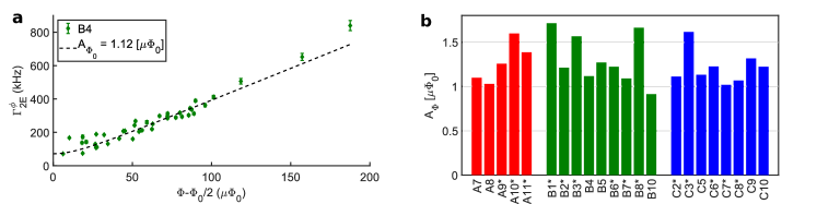
Figure 9: Flux noise amplitude. a, Echo pure dephasing rates of qubit B4 as a function of $\varPhi-\varPhi_{0}/2$. Fitting the measured data with 22 yields $A_{\Phi}=1.12\>\mu\Phi_{0}$ . b, Extracted amplitude of flux noise for different qubits in red for sample A, green for sample B and blue for sample C. We obtain almost the same flux noise amplitude $A_{\varPhi}=1.2\pm 0.2\>\mu\varPhi_{0}$ for all the qubits whether on sample A , B or C and including those with constrictions.

III.3 Dephasing at the optimal point

At the optimal point however, $\partial_{\Phi}\omega_{01}=0$ and therefore the qubit is immune to flux fluctuations to first order. Yet, $\partial_{\Phi}^{2}\omega_{01}=\left(\frac{2I_{p}}{\hbar}\right)^{2}/\left(2\pi\Delta\right)\neq 0$ and therefore second order flux noise should be taken into account. Unlike first order, deriving an analytical expression for 2nd order flux noise is not straight-forward. In this work, we performed numerical Monte Carlo simulations in Python [32]. The source code of this simulation can be found on Github [33].

III.3.1 Generation of flux noise trajectories

Microscopically, the flux noise is the sum of many independent uncorrelated sources, most likely spins on the surface of the loops [27]. Thus, it should be well described as a Gaussian variable. To simulate a flux noise trajectory in time, we first generate a series of $2\,n_{\text{FFT}}$ normally distributed real and imaginary random numbers $a_{i}+jb_{i}$ that will be used as Fourier components of the signal. These Fourier components are multiplied by an amplitude $A_{\Phi}\sqrt{\frac{n_{\text{FFT}}dt}{i}}$ where $dt$ is the time step unit of the simulation. Then, we apply an inverse fast Fourier transform in order to obtain a flux noise trajectory with power spectrum of $A_{\Phi}^{2}/f$. In the code, the class NoiseGen1OverF is a generator of pink noise. Attributes includes the time step unit $dt$, and the total number $n_{\text{FFT}}$ of samples to generate. The method generate is called to generate a single trajectory $\overrightarrow{\delta\Phi}=\left(\delta\Phi\left(t_{1}\right),\ldots,\delta\Phi\left(t_{n_{\text{FFT}}}\right)\right)$ around zero flux.

III.3.2 Ensemble averaging over noise trajectories

The next step of our simulation consists of ensemble averaging of a complex function over different trajectories. For Ramsey sequence, this complex function is

$$f_{R}\left(t\right)=\exp\left(i\int_{0}^{t}\omega_{01}\left(\Phi+\delta\Phi\left(u\right)\right)-\left\langle\omega_{01}\right\rangle du\right)$$

, where $\Phi$ is the flux threading the loop of the qubit. For Hahn-Echo sequence, the complex function is

$$f_{E}\left(t\right)=\exp\left(i\int_{0}^{t/2}\omega_{01}\left(\Phi+\delta\Phi\left(u\right)\right)du-i\int_{t/2}^{t}\omega_{01}\left(\Phi+\delta\Phi\left(u\right)\right)du\right)$$

In order to reduce the function call overheads, the function qb_plot_t2s_at performs the ensemble averaging by sampling the $n_{\text{FFT}}$-sized signal at fixed intervals, much like in a real experiment where ensemble repetitions occur in sequential order at a quasi-fixed period. To further increase the smoothness of the signal, we resample the same signal using the same period but with different time offsets.

⬇

for i in tqdm.tqdm(range(0, tobs_tstep, laziness)):#line 166

…# for different periodic offsets

In order to optimize the running complexity, the integral $\int_{t_{i}}^{t_{j}}\omega_{01}\left(\Phi+\delta\Phi\left(u\right)\right)du$ is calculated as a difference of pre-cached cumulative sums $\int_{0}^{t}\omega_{01}\left(\Phi+\delta\Phi\left(u\right)\right)du$:

$$\int_{t}^{t_{j}}\omega_{01}\left(\Phi+\delta\Phi\left(u\right)\right)du=\int_{0}^{t_{j}}\omega_{01}\left(\Phi+\delta\Phi\left(u\right)\right)du-\int_{0}^{t_{i}}\left(\Phi+\delta\Phi\left(u\right)\right)du$$

The pre-caching step is performed in only $O\left(n_{\text{FFT}}\right)$ complexity. To further speed up the whole algorithm, we perform the computation described above by using np.reshape commands instead of writing python for-loops, to exploit the faster speed of C-implemented numpy libraries.

Here is a list of important arguments of the function qb_plot_t2s_at:

1. t_step_ns corresponds to the time step unit $dt$

2. t_observation_ns, time interval on which the interpulse time delay will be varied. This is the X axis of the final plot.

3. t_total_ns, this is the total length of the pink signal, equal to $n_{\text{FFT}}dt$. The inverse is the resolution $df$ in frequency space.

4. t_cut_off_ns. Its inverse is the low frequency cutoff of the power spectrum. We assume white noise below this threshold.

The default sample program provided under the __main__ statement performs the following steps. First a typical flux qubit transition with parameters $\Delta,I_{p}$, under influence of pink noise of amplitude $A_{\Phi_{0}}$ is defined. Sanity checks on the calculations of the qubit’s first and second derivatives are performed (cf. equality c1 == c1_sp and c2 == c2_sp). Finally, after the averaging is complete, a plot of the ensemble averaged signal should pop up. The titles prints the decoherence times $\tau_{2E/R}$, defined by $\left|c\left(\tau_{2E/R}\right)\right|=1/e$.

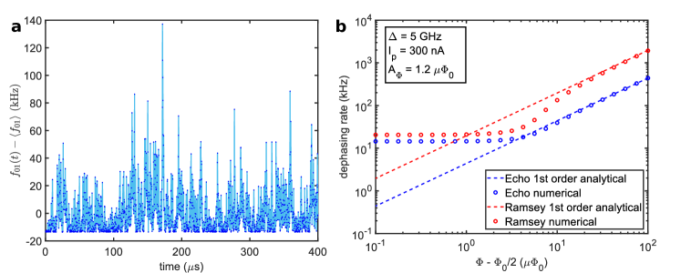
Figure 10: Calculated dephasing rates of a flux qubit. a, The frequency of a flux qubit at optimal point under influence of $1/f$ noise over a sub-sample of $400\ $\mathrm{\SIUnitSymbolMicro s}$$. The flux qubit parameters were chosen to be $\Delta=5\>\mathrm{GHz},I_{p}=300\>\mathrm{nA},A_{\varPhi}=1.2\>\mu\Phi_{0}$. The parameters of the numerical simulation are $t_{\text{step}}=200\text{ ns}$, $t_{\text{total}}=1\text{ s}$, $t_{\text{cut-off}}=0.2\text{ s}$. b, We numerically calculated the Ramsey and Echo dephasing rates and compared the results with analytical formula for first order flux noise. Away from the optimal point, analytical formula predict $\Gamma_{\varphi R}\sim 4.5\>\Gamma_{\varphi E}$ in agreement with the numerical simulations.

III.3.3 Empirical results for the second-order flux noise decoherence rates

Using the tool described above, and sweeping many different flux qubit parameters, we were able to establish the following empirical law for any second-order transition

$$\Gamma_{\varphi E}^{\left(2\right)}=14.4\frac{\partial^{2}f_{01}}{\partial\Phi^{2}}A_{\Phi_{0}}^{2}$$ (23)

where $f_{01}$ is the transition frequency.

For the particular case of the flux qubit at its optimal point, we obtain the formula used in the main article

$$\Gamma_{\varphi E}^{\left(2\right)}=56\frac{\left(I_{p}A_{\Phi_{0}}/h\right)^{2}}{\Delta}$$ (24)

IV Qubit and resonator parameters

Qubit ref.	$\Delta$ (GHz)	$I_{p}$ (nA)	$g$ (MHz)	$\chi$ (MHz)	$E_{J}$ (GHz)	$E_{J}/E_{C}$	$\alpha$	$\delta\Delta^{\text{geom}}$ (GHz)	$\delta\Delta^{n_{g}}$ (kHz)
A2	7.19	188	28	1.29	265	69	0.492	-1.09	78.4
A6	8.33	244	50	4.48	256	67	0.487	-0.51	95.1
A7	8.69	187	40	1.8	240	63	0.476	-1.34	136.3
A8	6.35	202	43	1.19	264	69	0.504	-0.83	94.5
A9	5.24	201	50	0.82	251	66	0.514	-1.25	154.6
A10	8.35	182	52	4.66	255	67	0.477	-1.54	88.1
A11	5.81	201	61	1.64	258	67	0.503	-1.49	110.1
B1	5.73	289	94	1.59	362	98	0.489	-1.61	3.7
B2	4.48	302	95	1.05	360	98	0.504	-1.36	5.0
B3	4.01	310	92	0.86	361	98	0.511	-1.24	5.4
B4	5.18	298	79	0.94	364	99	0.497	-1.30	4.0
B5	5.84	284	77	1.11	357	97	0.490	-1.46	4.3
B6	5.08	297	71	0.72	361	98	0.499	-1.27	4.5
B7	5.01	292	64	0.57	354	96	0.500	-1.31	5.4
B8	3.88	316	63	0.37	366	100	0.512	-1.17	4.8
B10	5.69	288	40	0.29	360	98	0.490	-1.53	4.0
C2	5.93	303	90	1.56	387	111	0.481	-1.54	1.0
C3	5.74	304	85	1.29	386	110	0.484	-1.47	1.1
C5	6.80	288	75	1.5	380	109	0.474	-1.52	1.1
C6	7.39	285	64	1.43	383	110	0.470	-1.50	0.9
C7	7.16	295	67	1.4	394	113	0.470	-1.54	0.7
C8	7.30	287	58	1.11	386	110	0.469	-1.61	0.8
C9	6.14	295	55	0.63	380	109	0.480	-1.48	1.2
C10	6.40	300	42	0.41	391	112	0.477	-1.57	0.8

Table 1: Qubit parameters. The values of $\Delta,$$I_{p}$, $g$ and $\chi$ were extracted from fit of the data as described in the main text. We simulated the design of each qubit with the electrostatic simulator of COMSOL in order to obtain the geometric capacitance matrix of the system. This matrix was corrected according to the prescriptions described herein above. Then, we fitted the parameters $E_{J}$ and $\alpha$ for each qubit assuming that the junctions have a capacitance per unit area $Cc=100\>\mathrm{fF/\mu m^{2}}$. The capacitance energy of the junctions is defined as $E_{c}=\frac{e^{2}}{2C_{J}}$. $\delta\Delta^{\text{geom}}$ is the difference between the value of the gap calculated with and without taking into account the geometric capacitance. As a rule of thumb, the geometric capacitance reduces the gap of the qubit by approximately 1-1.5 GHz. $\delta\Delta^{n_{g}}$is the charge modulation calculated for the fitted parameters $E_{J}$ and $\alpha$ of each qubit.

Resonator	Length ($\mathrm{\SIUnitSymbolMicro m}$)	$C_{C}$ (fF)	$f_{r}$ (GHz)	$Q_{tot}$	$\kappa\>\left(\mathrm{rad.s^{-1}}\right)$	$Q_{C}$	$Q_{int}$	$\bar{n}_{thermal}$
A	7250	5	7.756	1400	$3.5\times 10^{7}$	5500	1878	$8.88\times 10^{-4}$
B	5730		9.805	2800	$2.2\times 10^{7}$	3500	14000	$6.82\times 10^{-4}$
C	5730		9.850	2200	$2.8\times 10^{7}$	3500	5923	$6.78\times 10^{-4}$

Table 2: Resonator parameters. Length of the resonator, coupling capacitance $C_{C}$, bare frequency of the resonator $f_{r}$, quality factor $Q$ of the resonator, photon loss rate $\kappa$, coupling $Q_{C}$ and internal $Q_{int}$ quality factor of the resonator given by $\frac{1}{Q}=\frac{1}{Q_{C}}+\frac{1}{Q_{int}}$, estimated number of thermal photons in the resonator $\bar{n}_{thermal}$.

Qubit ref.	$\Gamma_{1}$ (kHz)	$\Gamma_{P}$ (kHz)	$\Gamma_{2E}^{\phi}$ (kHz)	$\Gamma_{2E}^{2nd}$ (kHz)	$\Gamma_{2E}^{photon}$ (kHz)
A2	1363	36	x	x	10
A6	354	143	x	x	131
A7	99	96	99	3	21
A8	38	17	46	4	9
A9	31	4	97	7	4
A10	330	245	440	6	134
A11	37	25	131	8	16
B1	84	4	169	24	12
B2	78	1	151	17	5
B3	82	0	123	33	4
B4	52	1	67	12	4
B5	67	1	115	13	6
B6	43	1	51	15	2
B7	55	1	217	11	1
B8	41	1	113	40	1
B10	59	3	113	7	0
C2	72	0	39	11	6
C3	54	2	77	24	4
C5	66	0	60	9	5
C6	82	1	78	9	5
C7	71	0	35	7	4
C8	86	12	42	7	3
C9	48	0	54	14	1
C10	67	0	32	12	0

Table 3: Decoherence rates. Measured relaxation rate $\Gamma_{1},$calculated Purcell decay rate $\Gamma_{P}$, measured pure echo dephasing rate at optimal point $\Gamma_{2E}^{\phi}$, calculated second order flux noise dephasing rate $\Gamma_{2E}^{2nd}$, calculated photon dephasing rate $\Gamma_{2E}^{photon}\approx 4\,\frac{\left(2\pi\chi\right)^{2}}{\kappa}\bar{n}_{thermal}\left(\bar{n}_{thermal}+1\right)$.

V Qubit fabrication and Room Temperature resistance measurements

The samples were fabricated on a $300\text{\,}\mathrm{\SIUnitSymbolMicro m}$ thick wafer of intrinsic silicon (resistivity $>10000\,\mathrm{\Omega}.\mathrm{cm}$) for sample A and on a thermally grown 5-nm width $\mathrm{SiO_{2}}$ layer for sample B and C. The oxide layer was grown at $800\text{\,}\mathrm{\SIUnitSymbolCelsius}$ for 20 minutes. This was immediately followed by a 60 minute anneal in nitrogen at the same temperature to reduce the fixed oxide charge. A $400\text{\,}\mathrm{\SIUnitSymbolCelsius}$ anneal in forming gas (Ar/H) concluded the process which was designed to passivate dangling bonds at the Si-$\mathrm{SiO_{2}}$ interface. Capacitance measurements on test devices yield an interface state density in the low $10^{10}${\mathrm{eV}}^{-1}\text{\,}{\mathrm{cm}}^{-2}$$. The fixed oxide charge is estimated to be in a similar range.

The silicon wafer was dipped into Piranha acid ($\mathrm{H_{2}SO_{4}:H_{2}O_{2}=4:1}$) for 5 min, rinsed in de-ionized water and immediately loaded into a Plassys MEB 550S evaporator. After one night of pumping, we evaporated 150 nm of Al onto the chip. Optical resist (AZ1505) was spun on the sample and large features $(>$1\text{\,}\mathrm{\SIUnitSymbolMicro m}$)$ were patterned with UV laser lithography. After development, the wafer was etched with Aluminium etchant, followed by cleaning in NMP overnight. We then spun a bilayer of methacrylic acid/ methyl methacrylate (EL7), evaporated 60 nm of Ge onto the chip and spun a high contrast electron-beam resist (CSAR 62) on the top of the germanium layer. The qubits were patterned by electron-beam lithography (50 kV, $660\text{\,}\mathrm{\SIUnitSymbolMicro C}\text{\,}{\mathrm{cm}}^{-2}$). The development took place in a 1:3 methyl isobutyl ketone (MIBK)/ isopropanol (IPA) solution for $240\text{\,}\mathrm{s}$, followed by 60s in IPA. The chip was then loaded into a Reactive Ion Etcher to perform plasma etching with SF6 in order to form a rigid germanium mask. We then developed the bilayer beneath with 1:3 MIBK/IPA solution for 90 s, followed by 60 s in IPA and cleaned the open regions by oxygen ashing for $240\text{\,}\mathrm{s}$. The sample was then loaded into a Plassys MEB 550S electron-beam evaporator and pumped overnight. We cooled the evaporator plate down to $-50\text{\,}\mathrm{\SIUnitSymbolCelsius}$ and evaporated a first layer of 25 nm of aluminium. We then performed a dynamic oxidation of $\mathrm{O_{2}/Ar}$ (15%-85%) at $P=20\>\mathrm{\mu bar}$ for 30 minutes. A second layer of 30 nm of aluminum was then evaporated at a temperature of $\sim$7\text{\,}\mathrm{\SIUnitSymbolCelsius}$$ followed by a static oxidation at $P=10\,\mathrm{mbar}$ for 10 minutes. This last step encapsulates the junctions with aluminium oxide and allows for a more controlled aging. An histogram of the junction resistances can be found in 11.

Figure 11: Room temperature resistance measurements. a, Microscope image showing 4 probe measurement of a test sample. b, AFM micrograph showing a close-up view on the test sample which consists of the two Josephson junctions in series. c, Resistance measurements of several unitary junctions for sample A (in red), B (in green) and C (in blue). The resistance of the unitary junctions is $614\pm 39\>\mathrm{\mathrm{\Omega}}$, $420\pm 7\>\mathrm{\mathrm{\Omega}}$, $398\pm 7\>\mathrm{\mathrm{\Omega}}$ for sample A,B and C respectively. d, Resistance measurements of several $\alpha$ junctions for sample A (in red), B (in green) and C (in blue). The resistance of the $\alpha$ junctions is $1185\pm 25\>\mathrm{\mathrm{\Omega}}$, $864\pm 12\>\mathrm{\mathrm{\Omega}}$, $857\pm 11\>\mathrm{\mathrm{\Omega}}$ for sample A,B and C respectively.

References

- [1] Hanhee Paik, D. I. Schuster, Lev S. Bishop, G. Kirchmair, G. Catelani, A. P. Sears, B. R. Johnson, M. J. Reagor, L. Frunzio, L. I. Glazman, S. M. Girvin, M. H. Devoret, and R. J. Schoelkopf. Observation of high coherence in josephson junction qubits measured in a three-dimensional circuit qed architecture. Phys. Rev. Lett., 107:240501, Dec 2011.
- [2] Alexander P. M. Place, Lila V. H. Rodgers, Pranav Mundada, Basil M. Smitham, Mattias Fitzpatrick, Zhaoqi Leng, Anjali Premkumar, Jacob Bryon, Andrei Vrajitoarea, Sara Sussman, Guangming Cheng, Trisha Madhavan, Harshvardhan K. Babla, Xuan Hoang Le, Youqi Gang, Berthold Jäck, András Gyenis, Nan Yao, Robert J. Cava, Nathalie P. de Leon, and Andrew A. Houck. New material platform for superconducting transmon qubits with coherence times exceeding 0.3 milliseconds. Nature Communications, 12(1), March 2021.
- [3] R. Barends, J. Kelly, A. Megrant, D. Sank, E. Jeffrey, Y. Chen, Y. Yin, B. Chiaro, J. Mutus, C. Neill, P. O’Malley, P. Roushan, J. Wenner, T. C. White, A. N. Cleland, and John M. Martinis. Coherent josephson qubit suitable for scalable quantum integrated circuits. Phys. Rev. Lett., 111:080502, Aug 2013.
- [4] Frank Arute, Kunal Arya, Ryan Babbush, Dave Bacon, Joseph C. Bardin, Rami Barends, Rupak Biswas, Sergio Boixo, Fernando G. S. L. Brandao, David A. Buell, Brian Burkett, Yu Chen, Zijun Chen, Ben Chiaro, Roberto Collins, William Courtney, Andrew Dunsworth, Edward Farhi, Brooks Foxen, Austin Fowler, Craig Gidney, Marissa Giustina, Rob Graff, Keith Guerin, Steve Habegger, Matthew P. Harrigan, Michael J. Hartmann, Alan Ho, Markus Hoffmann, Trent Huang, Travis S. Humble, Sergei V. Isakov, Evan Jeffrey, Zhang Jiang, Dvir Kafri, Kostyantyn Kechedzhi, Julian Kelly, Paul V. Klimov, Sergey Knysh, Alexander Korotkov, Fedor Kostritsa, David Landhuis, Mike Lindmark, Erik Lucero, Dmitry Lyakh, Salvatore Mandrà, Jarrod R. McClean, Matthew McEwen, Anthony Megrant, Xiao Mi, Kristel Michielsen, Masoud Mohseni, Josh Mutus, Ofer Naaman, Matthew Neeley, Charles Neill, Murphy Yuezhen Niu, Eric Ostby, Andre Petukhov, John C. Platt, Chris Quintana, Eleanor G. Rieffel, Pedram Roushan, Nicholas C. Rubin, Daniel Sank, Kevin J. Satzinger, Vadim Smelyanskiy, Kevin J. Sung, Matthew D. Trevithick, Amit Vainsencher, Benjamin Villalonga, Theodore White, Z. Jamie Yao, Ping Yeh, Adam Zalcman, Hartmut Neven, and John M. Martinis. Quantum supremacy using a programmable superconducting processor. Nature, 574(7779):505–510, October 2019.
- [5] S. A. Caldwell, N. Didier, C. A. Ryan, E. A. Sete, A. Hudson, P. Karalekas, R. Manenti, M. P. da Silva, R. Sinclair, E. Acala, N. Alidoust, J. Angeles, A. Bestwick, M. Block, B. Bloom, A. Bradley, C. Bui, L. Capelluto, R. Chilcott, J. Cordova, G. Crossman, M. Curtis, S. Deshpande, T. El Bouayadi, D. Girshovich, S. Hong, K. Kuang, M. Lenihan, T. Manning, A. Marchenkov, J. Marshall, R. Maydra, Y. Mohan, W. O’Brien, C. Osborn, J. Otterbach, A. Papageorge, J.-P. Paquette, M. Pelstring, A. Polloreno, G. Prawiroatmodjo, V. Rawat, M. Reagor, R. Renzas, N. Rubin, D. Russell, M. Rust, D. Scarabelli, M. Scheer, M. Selvanayagam, R. Smith, A. Staley, M. Suska, N. Tezak, D. C. Thompson, T.-W. To, M. Vahidpour, N. Vodrahalli, T. Whyland, K. Yadav, W. Zeng, and C. Rigetti. Parametrically activated entangling gates using transmon qubits. Phys. Rev. Applied, 10:034050, Sep 2018.
- [6] J. E. Mooij, T. P. Orlando, L. Levitov, Lin Tian, Caspar H. van der Wal, and Seth Lloyd. Josephson persistent-current qubit. Science, 285(5430):1036–1039, August 1999.
- [7] T. P. Orlando, J. E. Mooij, Lin Tian, Caspar H. van der Wal, L. S. Levitov, Seth Lloyd, and J. J. Mazo. Superconducting persistent-current qubit. Phys. Rev. B, 60:15398–15413, Dec 1999.
- [8] Caspar H. van der Wal, A. C. J. ter Haar, F. K. Wilhelm, R. N. Schouten, C. J. P. M. Harmans, T. P. Orlando, Seth Lloyd, and J. E. Mooij. Quantum superposition of macroscopic persistent-current states. Science, 290(5492):773–777, October 2000.
- [9] I. Chiorescu, Y. Nakamura, C. J. P. M. Harmans, and J. E. Mooij. Coherent quantum dynamics of a superconducting flux qubit. Science, 299(5614):1869–1871, March 2003.
- [10] D. Marcos, M. Wubs, J. M. Taylor, R. Aguado, M. D. Lukin, and A. S. Sørensen. Coupling nitrogen-vacancy centers in diamond to superconducting flux qubits. Phys. Rev. Lett., 105:210501, Nov 2010.
- [11] J. Twamley and S. D. Barrett. Superconducting cavity bus for single nitrogen-vacancy defect centers in diamond. Phys. Rev. B, 81:241202, Jun 2010.
- [12] Tom Douce, Michael Stern, Nicim Zagury, Patrice Bertet, and Pérola Milman. Coupling a single nitrogen-vacancy center to a superconducting flux qubit in the far-off-resonance regime. Phys. Rev. A, 92:052335, Nov 2015.
- [13] P. Bertet, I. Chiorescu, G. Burkard, K. Semba, C. J. P. M. Harmans, D. P. DiVincenzo, and J. E. Mooij. Dephasing of a superconducting qubit induced by photon noise. Phys. Rev. Lett., 95:257002, Dec 2005.
- [14] F. Yoshihara, K. Harrabi, A. O. Niskanen, Y. Nakamura, and J. S. Tsai. Decoherence of flux qubits due to flux noise. Phys. Rev. Lett., 97:167001, Oct 2006.
- [15] P. Forn-Díaz, J. Lisenfeld, D. Marcos, J. J. García-Ripoll, E. Solano, C. J. P. M. Harmans, and J. E. Mooij. Observation of the bloch-siegert shift in a qubit-oscillator system in the ultrastrong coupling regime. Phys. Rev. Lett., 105:237001, Nov 2010.
- [16] Jonas Bylander, Simon Gustavsson, Fei Yan, Fumiki Yoshihara, Khalil Harrabi, George Fitch, David G. Cory, Yasunobu Nakamura, Jaw-Shen Tsai, and William D. Oliver. Noise spectroscopy through dynamical decoupling with a superconducting flux qubit. Nature Physics, 7(7):565–570, May 2011.
- [17] M. Stern, G. Catelani, Y. Kubo, C. Grezes, A. Bienfait, D. Vion, D. Esteve, and P. Bertet. Flux qubits with long coherence times for hybrid quantum circuits. Phys. Rev. Lett., 113:123601, Sep 2014.
- [18] J.-L. Orgiazzi, C. Deng, D. Layden, R. Marchildon, F. Kitapli, F. Shen, M. Bal, F. R. Ong, and A. Lupascu. Flux qubits in a planar circuit quantum electrodynamics architecture: Quantum control and decoherence. Phys. Rev. B, 93:104518, Mar 2016.
- [19] Fei Yan, Simon Gustavsson, Archana Kamal, Jeffrey Birenbaum, Adam P Sears, David Hover, Ted J. Gudmundsen, Danna Rosenberg, Gabriel Samach, S Weber, Jonilyn L. Yoder, Terry P. Orlando, John Clarke, Andrew J. Kerman, and William D. Oliver. The flux qubit revisited to enhance coherence and reproducibility. Nature Communications, 7(1), November 2016.
- [20] Jarryd J. Pla, Kuan Y. Tan, Juan P. Dehollain, Wee H. Lim, John J. L. Morton, David N. Jamieson, Andrew S. Dzurak, and Andrea Morello. A single-atom electron spin qubit in silicon. Nature, 489(7417):541–545, September 2012.
- [21] See Supplementary Materials.
- [22] A. A. Houck, J. A. Schreier, B. R. Johnson, J. M. Chow, Jens Koch, J. M. Gambetta, D. I. Schuster, L. Frunzio, M. H. Devoret, S. M. Girvin, and R. J. Schoelkopf. Controlling the spontaneous emission of a superconducting transmon qubit. Phys. Rev. Lett., 101:080502, Aug 2008.
- [23] John M. Martinis, K. B. Cooper, R. McDermott, Matthias Steffen, Markus Ansmann, K. D. Osborn, K. Cicak, Seongshik Oh, D. P. Pappas, R. W. Simmonds, and Clare C. Yu. Decoherence in josephson qubits from dielectric loss. Phys. Rev. Lett., 95:210503, Nov 2005.
- [24] J. Krupka, J. Breeze, A. Centeno, N. Alford, T. Claussen, and L. Jensen. Measurements of permittivity, dielectric loss tangent, and resistivity of float-zone silicon at microwave frequencies. IEEE Transactions on Microwave Theory and Techniques, 54(11):3995–4001, November 2006.
- [25] Aaron D. O’Connell, M. Ansmann, R. C. Bialczak, M. Hofheinz, N. Katz, Erik Lucero, C. McKenney, M. Neeley, H. Wang, E. M. Weig, A. N. Cleland, and J. M. Martinis. Microwave dielectric loss at single photon energies and millikelvin temperatures. Applied Physics Letters, 92(11):112903, March 2008.
- [26] G. Ithier, E. Collin, P. Joyez, P. J. Meeson, D. Vion, D. Esteve, F. Chiarello, A. Shnirman, Y. Makhlin, J. Schriefl, and G. Schön. Decoherence in a superconducting quantum bit circuit. Phys. Rev. B, 72:134519, Oct 2005.
- [27] Jochen Braumüller, Leon Ding, Antti P. Vepsäläinen, Youngkyu Sung, Morten Kjaergaard, Tim Menke, Roni Winik, David Kim, Bethany M. Niedzielski, Alexander Melville, Jonilyn L. Yoder, Cyrus F. Hirjibehedin, Terry P. Orlando, Simon Gustavsson, and William D. Oliver. Characterizing and optimizing qubit coherence based on squid geometry. Phys. Rev. Applied, 13:054079, May 2020.
- [28] R. W. Simmonds, K. M. Lang, D. A. Hite, S. Nam, D. P. Pappas, and John M. Martinis. Decoherence in josephson phase qubits from junction resonators. Phys. Rev. Lett., 93:077003, Aug 2004.
- [29] J. Eroms, L. C. van Schaarenburg, E. F. C. Driessen, J. H. Plantenberg, C. M. Huizinga, R. N. Schouten, A. H. Verbruggen, C. J. P. M. Harmans, and J. E. Mooij. Low-frequency noise in josephson junctions for superconducting qubits. Applied Physics Letters, 89(12):122516, September 2006.
- [30] Emanuele Albertinale, Léo Balembois, Eric Billaud, Vishal Ranjan, Daniel Flanigan, Thomas Schenkel, Daniel Estève, Denis Vion, Patrice Bertet, and Emmanuel Flurin. Detecting spins by their fluorescence with a microwave photon counter. Nature, 600(7889):434–438, December 2021.
- [31] M. Bal, M. H. Ansari, J.-L. Orgiazzi, R. M. Lutchyn, and A. Lupascu. Dynamics of parametric fluctuations induced by quasiparticle tunneling in superconducting flux qubits. Phys. Rev. B, 91:195434, May 2015.
- [32] Paul Brookes, Tikai Chang, Marzena Szymanska, Eytan Grosfeld, Eran Ginossar, and Michael Stern. Protection of quantum information in a chain of josephson junctions. Phys. Rev. Applied, 17:024057, Feb 2022.
- [33] https://github.com/teacup123123/pink_flux_noise_analysis.