Task-oriented Self-supervised Learning for Anomaly Detection in Electroencephalography

Abstract

Accurate automated analysis of electroencephalography (EEG) would largely help clinicians effectively monitor and diagnose patients with various brain diseases. Compared to supervised learning with labelled disease EEG data which can train a model to analyze specific diseases but would fail to monitor previously unseen statuses, anomaly detection based on only normal EEGs can detect any potential anomaly in new EEGs. Different from existing anomaly detection strategies which do not consider any property of unavailable abnormal data during model development, a task-oriented self-supervised learning approach is proposed here which makes use of available normal EEGs and expert knowledge about abnormal EEGs to train a more effective feature extractor for the subsequent development of anomaly detector. In addition, a specific two-branch convolutional neural network with larger kernels is designed as the feature extractor such that it can more easily extract both larger-scale and small-scale features which often appear in unavailable abnormal EEGs. The effectively designed and trained feature extractor has shown to be able to extract better feature representations from EEGs for development of anomaly detector based on normal data and future anomaly detection for new EEGs, as demonstrated on three EEG datasets. The code is available at https://github.com/ironing/EEG-AD.

1 Introduction

Electroencephalography (EEG) is one type of brain imaging technique and has been widely used to monitor and diagnose brain status of patients with various brain diseases (e.g., epilepsy) [12, 11, 16, 10, 2]. EEG data typically consists of multiple sequences (or channels) of waveform signals, with each sequence obtained by densely sampling electrical signals of brain activities from a unique electrode attached to a specific position on patient’s head surface. While brain activities can be recorded by EEG equipment over hours or even days, clinicians often analyze EEG data at the level of seconds, considering that cycles of most brain activities varies between 0.5Hz and 30Hz. Therefore, it is very tedious to manually analyze long-term EEG data and automated analysis of EEG would largely alleviate clinician efforts in timely monitoring patient statuses.

Currently, most automated analyses of EEGs focus on specific diseases [17, 8, 1], where labelled EEGs at the onset of disease and normal (healthy) status are collected to train a classifier for prediction of patient status at the level of seconds. However, such automated systems can only help analyze specific diseases and would fail to recognize novel unhealthy statuses which do not appear during classifier training. In contrast, developing an anomaly detector based on only normal EEGs has the potential to detect any possible unhealthy status (i.e., anomaly) in new EEG data. While multiple anomaly detection strategies have been developed for both natural and medical image analyses [22, 24], including statistical approaches [13, 18], discriminative approaches [4, 25] reconstruction approaches [27, 19] and self-supervised learning approaches [5, 15], very limited studies have been investigated on anomaly detection based on normal EEGs only [26]. Furthermore, all these strategies build anomaly detectors without considering any property of anomaly due to absence of abnormal data during model development. One exception is the recently proposed CutPaste method for anomaly detection in natural images [14], where simulated abnormal images were generated by cutting and pasting small image patches in normal images and then used to help train a more effective feature extractor and anomaly detector.

Inspired by the CutPaste method, we propose a novel task-oriented self-supervised learning approach to train an effective feature extractor based on normal EEG data and expert knowledge (key properties including increased amplitude and unusual frequencies) about unavailable abnormal EEGs. In addition, a specific two-branch convolutional neural network (CNN) with larger kernels is designed for effective extraction of both small-scale and large-scale features, such that the CNN feature extractor can be trained to extract features of both normal and abnormal EEGs. The feature extractor with more powerful representation ability can help establish a better anomaly detector. State-of-the-art anomaly detection performance was obtained on one internal and two public EEG datasets, confirming the effectiveness of the proposed approach.

2 Methodology

In this study, we try to solve the problem of anomaly detection in EEGs when only normal EEG data is available for training. A two-stage framework is proposed here, where the first stage aims to a train a feature extractor using a novel self-supervised learning method, and the second stage can adopt any existing generative or discriminative method to establish an anomaly detector based on the feature representations from the well-trained feature extractor.

2.1 Task-oriented self-supervised learning

Various self-supervised learning (SSL) strategies have been proposed to train feature extractors for downstream tasks in both natural and medical image analysis. To make a feature extractor more generalizable for downstream tasks, existing SSL strategies are often designed purposely without regard to any specific downstream task. That means, SSL strategies often do not consider characteristics in specific downstream tasks. However, when applying any such SSL technique to an anomaly detection task, the feature extractor based on only normal data would less likely learn to extract features of abnormal data, and therefore may negatively affect model performance in the subsequent anomaly detection task.

Different from most SSL strategies, a novel SSL strategy is proposed here to train a feature extractor which can extract features of both normal and abnormal EEG data. Specifically, considering that abnormal EEGs are characterized by increased wave amplitude or temporally slowed or abrupt wave signals, two special transformations are designed to generate simulated abnormal EEG data. One transformation is to temporally locally increase amplitude of normal EEG signals (Figure 1, Middle), and the other transformation is to temporally increase or decrease the frequency of normal EEG signals (Figure 1, Right). These amplitude-abnormal and frequency-abnormal data, together with original normal EEGs, form a 3-class dataset for the training of a 3-class CNN classifier. The feature extractor part of the well-trained classifier would be expected to learn to extract features of both normal and (simulated) abnormal EEGs. While the simulated abnormal data are different from real abnormal EEGs, empirical evaluations show the feature extractor trained with simulated abnormal EEGs helps improve the performance of anomaly detection significantly.

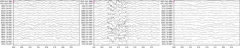
Figure 1: Transformation of normal EEG (Left) to generate simulated amplitude-abnormal (Middle) and frequency-abnormal (Right) EEGs. One EEG data consists of multiple sequences (channels, y-axis) of wave signals. x-axis: time (seconds).

2.1.1 Generation of self-labeled abnormal EEG data:

Denote a normal EEG data by a matrix $\mathbf{X}\in\mathbb{R}^{K\times L}$, where $K$ represents the number of channels (sequences) and $L$ represents the length of each sequence. To generate an amplitude-abnormal EEG data based on $\mathbf{X}$, a scalar amplitude factor $\alpha$ is firstly sampled from a predefined range $[\alpha_{l},\alpha_{h}]$ where $1<\alpha_{l}<\alpha_{h}$, followed by sampling a segment length $w$ from a predefined sequence segment range $[w_{l},w_{h}]$ where $1<w_{l}<w_{h}<L$. Then $w$ consecutive columns in $\mathbf{X}$ were randomly chosen, with each element in these columns multiplied by the amplitude factor $\alpha$. Such transformed EEG data with modified $w$ consecutive columns can be used as a simulated amplitude-abnormal EEG data (Figure 1, Middle). On the other hand, to generate a lower-frequency abnormal EEG data based on $\mathbf{X}$, a frequency scalar factor $\omega$ is firstly randomly sampled from a predefined range $[\omega_{l},\omega_{h}]$ where $1<\omega_{l}<\omega_{h}$, and then each sequence (row) of signals in $\mathbf{X}$ is linearly interpolated (i.e., upsampled) by the factor $\omega$ to generate an elongated EEG data $\mathbf{X}^{\prime}\in\mathbb{R}^{K\times L^{\prime}}$, where $L^{\prime}=\lfloor\omega L\rfloor$ is the largest number which is equal to or smaller than $\omega L$. One frequency-abnormal EEG data can be generated by randomly choosing $L$ consecutive columns from $\mathbf{X}^{\prime}$. Similarly, to alternatively generate a higher-frequency abnormal EEG data from $\mathbf{X}$, the frequency scalar factor $\omega^{\prime}$ is firstly randomly sampled from another predefined range $[\omega^{\prime}_{l},\omega^{\prime}_{h}]$ where $0<\omega^{\prime}_{l}<\omega^{\prime}_{h}<1$, and then each row of signals in $\mathbf{X}$ is down-sampled by the factor $\omega^{\prime}$ to generate a shortened EEG data. The shortened EEG data is then concatenated by itself multiple times along the temporal (i.e., row) direction to obtain a temporary EEG data $\mathbf{X}^{\prime\prime}\in\mathbb{R}^{K\times L^{\prime\prime}}$ where $L^{\prime\prime}=\lfloor\omega^{\prime}L\rfloor\cdot\lceil\frac{1}{\omega^{\prime}}\rceil\geq L$. One higher-frequency abnormal EEG data can be obtained by randomly choosing $L$ consecutive columns from $\mathbf{X}^{\prime\prime}$ (when $L^{\prime\prime}>L$) or just be $\mathbf{X}^{\prime\prime}$ (when $L^{\prime\prime}=L$).

Using these simple transformations and based on multiple normal EEG data, two classes of self-labeled abnormal data will be generated, with one class representing anomaly in amplitude, and the other representing anomaly in frequency. Although more complex transformations can be designed to generate more realistic amplitude- and frequency-abnormal EEGs, empirical evaluations show the simple transformations are sufficient to help train an anomaly detector for EEGs.

Figure 2: The two-branch architecture for feature extractor training. The second branch (lower part) consists of only one convolutional layer for extraction of small-scale features. The part in the blue dotted box is the feature extractor.

2.1.2 Architecture design for feature extractor:

To train a feature extractor with more powerful representation ability, we designed a specific CNN classifier based on the ResNet34 backbone (Figure 2). Considering that two adjacent channels (rows) in the EEG data do not indicate spatial proximity between two brain regions, one-dimensional (1D) convolutional kernels are adopted to learn to extract features from each channel over convolutional layers as in previous studies [9]. However, different from the previously proposed 1D kernels of size $1\times 3$, kernels of longer size in time (i.e., $1\times 7$ here) is adopted in this study. Such longer kernels are used considering that lower-frequency features may last for a a longer period (i.e., longer sequence segment) in EEGs and therefore would not be well captured by shorter kernels even over multiple convolutional layers. On the other hand, considering that some other anomalies in EEGs may last for very short time and therefore such abnormal features may be omitted after multiple times of pooling or down-sampling over layers, we propose adding a shortcut branch from the output of the first convolutional layer to the penultimate layer. Specifically, the shortcut branch consists of only one convolutional layer in which each kernel is two-dimensional (i.e., number of EEG channels $\times$ 7) in order to capture potential correlation across all the channels in short time interval. By combining outputs from the two branches, both small-scale and large-scale features in time would be captured. The concatenated features are fed to the last fully connected layer for prediction of EEG category. The output of the classifier consists of three values, representing the prediction probability of ‘normal EEG’, ‘amplitude-abnormal EEG’, and ‘frequency-abnormal EEG’ class, respectively.

The feature extractor plus the 3-class classifier head can be trained by minimizing the cross-entropy loss on the 3-class training set. After training, the classifier head is removed and the feature extractor is used to extract features from normal EEGs for the development of anomaly detector. Since the feature extractor is trained without using real abnormal EEGs and the simulated abnormal EEGs are transformed from normal EEGs and self-labelled, the training is an SSL process. The SSL is task-oriented because it considers the characteristics (i.e., crucial anomaly properties in both amplitude and frequency of abnormal EEGs) in the subsequent specific anomaly detection task. The feature extractor based on such task-oriented SSL is expected to be able to extract features of both normal and abnormal EEGs for more accurate anomaly detection.

2.2 Anomaly detection

While in principle any existing anomaly detection strategy can be applied based on feature representations of normal EEGs from the well-trained feature extractor, here the generative approach is adopted to demonstrate the effectiveness of the proposed two-stage framework considering that a large amount of normal EEG data are available to estimate the distribution of normal EEGs in the feature space. Note discriminative approaches like one-class SVM may be a better choice if normal data is limited. As one simple generative approach, multivariate Gaussian distribution $\mathcal{G}(\mbox{\boldmath$\mu$},\mathbf{\Sigma})$ is used here to represent the distribution of normal EEGs, where the mean $\mu$ and the covariance matrix $\mathbf{\Sigma}$ are directly estimated from the feature vectors of all normal EEGs in the training set, with each vector being the output of the feature extractor given a normal EEG input.

With the Gaussian model $\mathcal{G}(\mbox{\boldmath$\mu$},\mathbf{\Sigma})$, the degree of abnormality for any new EEG data $\mathbf{z}$ can be estimated based on the Mahalanobis distance between the mean $\mu$ and the feature representation $f(\mathbf{z})$ of the new data $\mathbf{z}$, i.e.,

$$A(\mathbf{z})=\sqrt{(f(\mathbf{z})-\mbox{\boldmath$\mu$})^{\top}\Sigma^{-1}(f(\mathbf{z})-\mbox{\boldmath$\mu$})}\,.$$ (1)

Larger $A(\mathbf{z})$ score indicates that $\mathbf{z}$ is more likely abnormal, and vice versa.

3 Experiments and results

Table 1: The statistics of three EEG datasets.

Dataset	Sampling rate	Channels	Patients	Normal EEGs (seconds)	Abnormal EEGs (seconds)
Internal	1024	19	50	30008	14402
CHB-MIT	256	18	21	70307	11506
UPMC	400	16	4	9116	1087

Experimental settings: Three EEG datasets were used to evaluate the proposed approach, including the public Children’s Hospital Boston–Massachusetts Institute of Technology Database (‘CHB–MIT’) [21] and the UPenn and Mayo Clinic’s Seizure Detection Challenge dataset (‘UPMC’) [23], and an internal dataset from a national hospital (‘Internal’). See Table 1 for details. While only the ictal stage of seizure is included as anomaly in UPMC, both ictal and various interictal epileptiform discharges (IEDs) were included in Internal and CHB-MIT. Particularly, the abnormal waveforms in Internal include triphasic waves, spike-and-slow-wave complexes, sharp-and-slow-wave complex, multiple spike-and-slow-wave complexes, multiple sharp-and-slow-wave complex and ictal discharges. 2 out of 23 patients were removed from CHB–MIT due to irregular channel naming and electrode positioning. For normal EEG recordings lasting for more than one hour in CHB-MIT, only the first hour of normal EEG recordings were included to partly balance data size across patients. In UPMC, only dog data were used because of inconsistent recording locations across human patients. For CHB–MIT and Internal, each original EEG recording was cut into short segments of fixed length (3 seconds in experiments). For UPMC, one-second short segments have been provided by the organizer. Each short segment was considered as one EEG data during model development and evaluation. Therefore the size of each EEG data is [number of channels, sampling rate $\times$ segment duration]. For each dataset, signal amplitude in EEG data was normalized to the range $[0,1]$ based on the minimum and maximum signal values in the dataset.

On each dataset, while all abnormal EEG data were used for testing, normal EEG data were split into training and test parts in two ways. One way (Setting I, default choice) is to randomly choose the same number of normal EEGs as that of abnormal EEGs for testing and the remaining is for training, without considering patient identification of EEGs. The other (Setting II, subject level) is to split patients with the cross-validation strategy, such that all normal EEGs of one patient were used either for training or test at each round of cross validation.

In training the 3-class classifier, for each batch of 64 normal EEGs, correspondingly 64 amplitude-abnormal EEGs and 64 frequency-abnormal (32 higher-frequency and 32 lower-frequency) EEGs were generated (see Section 2.1.1). Adam optimizer with learning rate 0.0001 and weight decay coefficient 0.00003 were adopted, and training was consistently observed convergent within 300 epochs. $[\alpha_{l},\alpha_{h}]=[2.0,4.0]$, $[w_{l},w_{h}]=[4,L]$, $[\omega_{l},\omega_{h}]=[2,4]$, and $[\omega^{\prime}_{l},\omega^{\prime}_{h}]=[0.1,0.5]$. The ranges of amplitude and frequency scalar factors were determined based on expert knowledge about potential changes of abnormal brain wave compared to normal signals. The area under ROC curve (AUC) and its average and standard deviation over five runs (Setting I) or multiple rounds of validation (Setting II), the equal error rate (EER), and F1-score (at EER) were reported.

Effectiveness evaluation: Our method was compared with well-known anomaly detection methods including the one-class SVM (OC-SVM) [20], the statistical kernel density estimation (KDE), and the autoencoder (AE) [7], the recently proposed methods Multi-Scale Convolutional Recurrent Encoder-Decoder (MSCRED) [28] and Unsupervised Anomaly Detection (USAD) [3] for multivariate time series, and the recently proposed SSL methods for anomaly detection, including ScaleNet [26] and CutPaste [14]. Note that ScaleNet [26] uses frequencies of normal EEGs at multiple scales to help detect abnormal EEGs, without considering any characteristics in abnormal EEGs. Similar efforts were taken to tune relevant hyper-parameters for each method. In particular, to obtain feature vector input for OC-SVM and KDE, every row in each EEG data was reduced to a 64-dimensional vector by principal component analysis (PCA) based on all the row vectors of all normal EEGs in each dataset, and then all the dimension-reduced rows were concatenated as the feature representation of the EEG data. For AE, the encoder consists of three convolutional layers and one fully connected (FC) layer, and symmetrically the decoder consists of one FC and three deconvolutional layers. For CutPaste, each normal EEG in each training set is considered as a gray image of size $K\times L$ pixels, and the suggested hyper-parameters from the original study [14] were adopted for model training. For ScaleNet, the method was re-implemented with suggested hyper-parameters [26]. As Table 2 shows, on all three datasets, our method (last row) outperforms all the baselines by a large margin. Consistently, as Figure 3 (Left) demonstrates, our method performed best as well at the subject level (i.e., Setting II), although the performance decreases a bit due to the more challenging setting. All these results clearly confirm the effectiveness of our method for anomaly detection in EEGs.

Table 2: Performance comparison on three datasets with Setting I. Bold face indicates the best, and italic face for the second best. Standard deviations are in brackets.

Method		Internal				CHB-MIT			UPMC
	EER$\downarrow$	F1$\uparrow$	AUC$\uparrow$		EER$\downarrow$	F1$\uparrow$	AUC$\uparrow$		EER$\downarrow$	F1$\uparrow$	AUC$\uparrow$
OC-SVM	0.30(0.008)	0.71(0.008)	0.75(0.02)		0.33(0.001)	0.69(0.001)	0.73(0.003)		0.33(0.01)	0.51(0.02)	0.74(0.01)
KDE	0.24(0.001)	0.76(0.001)	0.87(0.001)		0.32(0.002)	0.69(0.002)	0.75(0.003)		0.24(0.003)	0.70(0.004)	0.83(0.003)
AE	0.35(0.01)	0.65(0.01)	0.69(0.02)		0.46(0.007)	0.54(0.007)	0.56(0.01)		0.32(0.02)	0.61(0.02)	0.75(0.02)
MSCRED	0.37(0.02)	0.64(0.03)	0.67(0.03)		0.34(0.03)	0.67(0.03)	0.72(0.03)		0.28(0.02)	0.70(0.02)	0.76(0.02)
USAD	0.25(0.02)	0.76(0.02)	0.83(0.02)		0.30(0.02)	0.69(0.03)	0.79(0.02)		0.24(0.02)	0.75(0.02)	0.82(0.02)
ScaleNet	0.18(0.01)	0.82(0.01)	0.90(0.01)		0.26(0.03)	0.73(0.03)	0.81(0.03)		0.20(0.03)	0.75(0.03)	0.89(0.03)
CutPaste	0.26(0.02)	0.74(0.02)	0.83(0.03)		0.26(0.01)	0.74(0.01)	0.83(0.01)		0.21(0.01)	0.74(0.01)	0.87(0.006)
Ours	0.11(0.01)	0.89(0.01)	0.95(0.004)		0.16(0.01)	0.84(0.02)	0.92(0.02)		0.13(0.007)	0.83(0.01)	0.95(0.006)

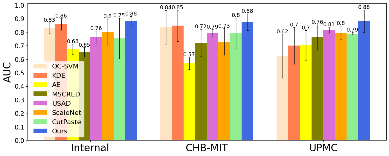
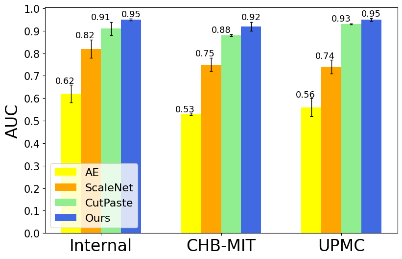
Figure 3: Performance comparison at the subject level (i.e., Setting II) on each dataset (Left), and the ablation study of the feature extractor training (Right). AUC values were included in figure for each method. Vertical line: standard deviation.

Ablation studies: To specifically confirm the effectiveness of the proposed task-oriented SSL strategy in training a feature extractor for EEG anomaly detection, an ablation study is performed by replacing this SSL strategy with several other SSL strategies, including (1) training an autoencoder and then keeping the encoder part as the feature extractor, (2) training a ScaleNet and then keeping its feature extractor part whose structure is the same as the proposed one, and (3) contrastive learning of the proposed two-branch feature extractor using the well-known SimCLR method [6]. As Figure 3 (Right) shows, compared to these SSL strategies which do not consider any property of anomalies in EEGs, our SSL strategy performs clearly better on all three datasets.

Another ablation study was performed to specifically confirm the role of the proposed two-branch backbone and self-labeled abnormal EEGs during feature extractor training. From Table 3, it is clear that the inclusion of the two types of simulated anomalies boosted the performance from AUC=0.71 to 0.93, and additional inclusion of the second branch (‘Two-branch’) and change of kernel size from $1\times 3$ to $1\times 7$ (‘Larger kernel’) further improved the performance.

In addition, one more evaluation showed the proposed simple transformations (based on simulated anomalies in frequency and amplitude individually) performed better than the more complex transformations (based on combinations of simulated abnormal frequency and amplitude), with AUC 0.954 vs. 0.901 on dataset Internal, 0.924 vs. 0.792 on CHB-MIT, and 0.952 vs. 0.918 on UPMC. Although simulated combinations of anomalies could be more realistic, they may not cover all possible anomalies in real EEGs and so the feature extractor could be trained to extract features of only the limited simulated complex anomalies. In contrast, with simple transformations, the feature extractor is trained to extract features which are discriminative enough between normal EEGs and simulated abnormal EEGs based on only abnormal frequency or amplitude features, therefore more powerful and effective in extracting discriminative features.

Table 3: The effect of simulated anomaly classes and the two-branch architecture on anomaly detection with ‘Internal’ dataset.

Amplitude-abnormal		✓		✓	✓	✓	✓
Frequency-abnormal			✓	✓	✓	✓	✓
Two-branch					✓		✓
Larger kernel						✓	✓
AUC	0.71(0.04)	0.91(0.001)	0.89(0.01)	0.93(0.01)	0.94(0.006)	0.94(0.005)	0.95(0.004)

Sensitivity studies: The proposed task-oriented SSL strategy is largely insensitive to the hyper-parameters for generating simulated abnormal EEGs. For example, as shown in Figure 4, when respectively varying the range $[\alpha_{l},\alpha_{h}]$ from $[2.0,3.0]$ to $[2.0,7.0]$, the range $[w_{l},w_{h}]$ from $[4,L/5]$ to $[4,L]$, the range $[\omega_{l},\omega_{h}]$ from $[2,3]$ to $[2,7]$, and the range $[\omega^{\prime}_{l},\omega^{\prime}_{h}]$ from $[0.1,0.4]$ to $[0.1,0.8]$, the final anomaly performance changes in a relatively small range and all of them are clearly better than the baselilne methods. These results support that the proposed task-oriented SSL strategy is quite stable in improving anomaly detection.

In addition, it is expected the proposed SSL strategy works stably even when injecting incompatible transformations. For example, during training the feature extractor, when a proportion ($5\%$, $10\%$, $15\%$, $20\%$) of simulated abnormal EEGs were replaced by fake abnormal EEGs (each fake EEG randomly selected from real normal EEGs but used as abnormal), the AUC is respectively 0.927, 0.916, 0.898, and 0.883 on Internal, lower than original 0.954 but still kept at high level.

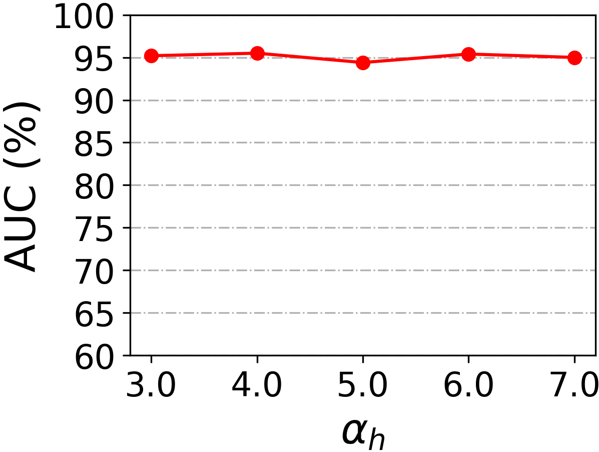
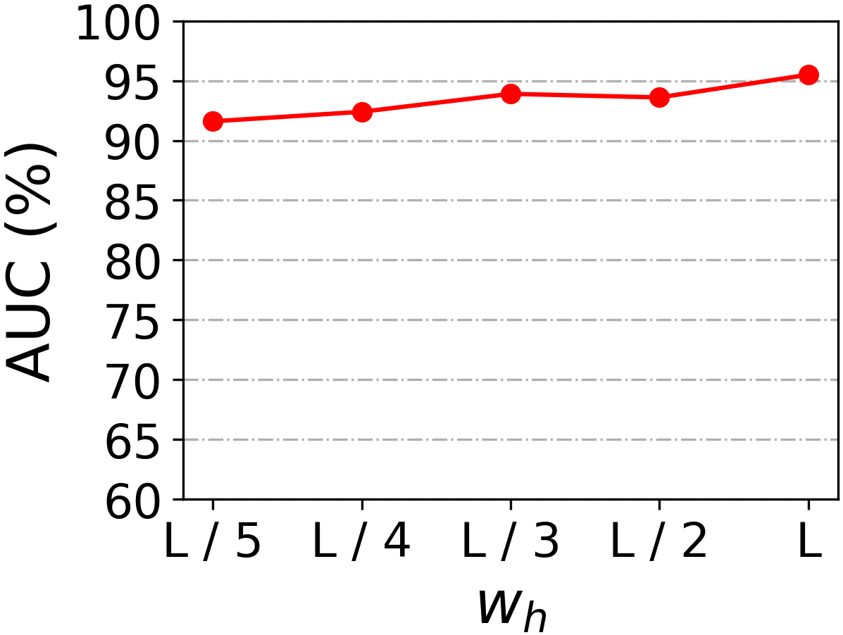
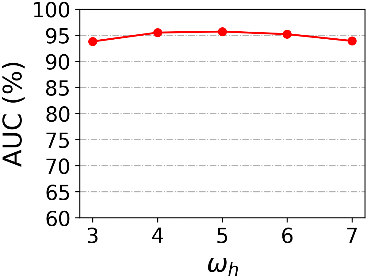
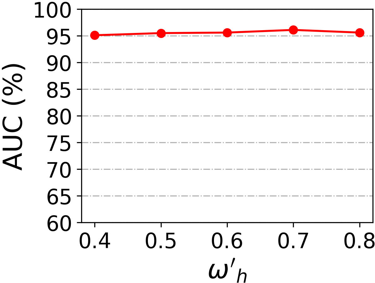
Figure 4: Sensitivity study of hyper-parameters.

4 Conclusion

In this study, we propose a two-stage framework for anomaly detection in EEGs based on normal EEGs only. The proposed task-oriented self-supervised learning together with the two-branch feature extractor from the first stage was shown to be effective in helping improve the performance of the anomaly detector learned at the second stage. This suggests that although only normal data are available for anomaly detection in some scenarios, transformation of normal data with embedded key properties of anomalies may generate simulated abnormal data which can be used to greatly help develop a more effective anomaly detector.

Acknowledgments. This work is supported by NSFCs (No. 62071502, U1811461), the Guangdong Key Research and Development Program (No. 2020B1111190001), and the Meizhou Science and Technology Program (No. 2019A0102005).

References

- [1] Achilles, F., Tombari, F., Belagiannis, V., Loesch, A.M., Noachtar, S., Navab, N.: Convolutional neural networks for real-time epileptic seizure detection. Computer methods in biomechanics and biomedical engineering. Imaging & visualization 6, 264–269 (2018)
- [2] Alturki, F.A., AlSharabi, K., Abdurraqeeb, A.M., Aljalal, M.: EEG signal analysis for diagnosing neurological disorders using discrete wavelet transform and intelligent techniques. Sensors 20(9), 2505 (2020)
- [3] Audibert, J., Michiardi, P., Guyard, F., Marti, S., Zuluaga, M.A.: Usad: Unsupervised anomaly detection on multivariate time series. In: KDD. pp. 3395–3404 (2020)
- [4] Chalapathy, R., Menon, A.K., Chawla, S.: Anomaly detection using one-class neural networks. arXiv preprint arXiv:1802.06360 (2018)
- [5] Chen, L., Bentley, P., Mori, K., Misawa, K., Fujiwara, M., Rueckert, D.: Self-supervised learning for medical image analysis using image context restoration. Medical Image Analysis 58, 101539–101539 (2019)
- [6] Chen, T., Kornblith, S., Norouzi, M., Hinton, G.: A simple framework for contrastive learning of visual representations. In: ICML. pp. 1597–1607 (2020)
- [7] Chen, Z., Yeo, C.K., Lee, B.S., Lau, C.T.: Autoencoder-based network anomaly detection. In: WTS (2018)
- [8] Craley, J., Johnson, E., Venkataraman, A.: A novel method for epileptic seizure detection using coupled hidden markov models. In: MICCAI (2018)
- [9] Dai, G., Zhou, J., Huang, J., Wang, N.: Hs-cnn: a cnn with hybrid convolution scale for motor imagery classification. Journal of neural engineering 17, 016025 (2020)
- [10] Dhar, P., Garg, V.K.: Brain-related diseases and role of electroencephalography (EEG) in diagnosing brain disorders. In: ICT Analysis and Applications, pp. 317–326 (2021)
- [11] Fiest, K.M., Sauro, K.M., Wiebe, S., Patten, S.B., Kwon, C.S., Dykeman, J., Pringsheim, T., Lorenzetti, D.L., Jetté, N.: Prevalence and incidence of epilepsy: A systematic review and meta-analysis of international studies. Neurology 88(3), 296–303 (2017)
- [12] Gemein, L.A., Schirrmeister, R.T., Chrabąszcz, P., Wilson, D., Boedecker, J., Schulze-Bonhage, A., Hutter, F., Ball, T.: Machine-learning-based diagnostics of EEG pathology. NeuroImage 220, 117021 (2020)
- [13] Jia, W., Shukla, R.M., Sengupta, S.: Anomaly detection using supervised learning and multiple statistical methods. In: ICML (2019)
- [14] Li, C.L., Sohn, K., Yoon, J., Pfister, T.: Cutpaste: Self-supervised learning for anomaly detection and localization. In: CVPR. pp. 9664–9674 (2021)
- [15] Li, Z., Li, N., Jiang, K., Ma, Z., Wei, X., Hong, X., Gong, Y.: Superpixel masking and inpainting for self-supervised anomaly detection. In: BMVC (2020)
- [16] Megiddo, I., Colson, A., Chisholm, D., Dua, T., Nandi, A., Laxminarayan, R.: Health and economic benefits of public financing of epilepsy treatment in india: An agent-based simulation model. Epilepsia 57, 464–474 (2016)
- [17] Pérez-García, F., Scott, C., Sparks, R., Diehl, B., Ourselin, S.: Transfer learning of deep spatiotemporal networks to model arbitrarily long videos of seizures. In: MICCAI. pp. 334–344 (2021)
- [18] Rippel, O., Mertens, P., Merhof, D.: Modeling the distribution of normal data in pre-trained deep features for anomaly detection. In: ICPR (2021)
- [19] Schlegl, T., Seeböck, P., Waldstein, S.M., Langs, G., Schmidt-Erfurth, U.: f-anogan: Fast unsupervised anomaly detection with generative adversarial networks. Medical Image Analysis 54, 30–44 (2019)
- [20] Schölkopf, B., Williamson, R.C., Smola, A.J., Shawe-Taylor, J., Platt, J.: Support vector method for novelty detection. In: NeurIPS (1999)
- [21] Shoeb, A.H.: Application of machine learning to epileptic seizure onset detection and treatment. Ph.D. thesis, Massachusetts Institute of Technology (2009)
- [22] Shvetsova, N., Bakker, B., Fedulova, I., Schulz, H., Dylov, D.V.: Anomaly detection in medical imaging with deep perceptual autoencoders. IEEE Access 9, 118571–118583 (2021)
- [23] Temko, A., Sarkar, A., Lightbody, G.: Detection of seizures in intracranial EEG: Upenn and mayo clinic’s seizure detection challenge. In: EMBC. pp. 6582–6585 (2015)
- [24] Tian, Y., Pang, G., Liu, F., Chen, Y., Shin, S.H., Verjans, J.W., Singh, R., Carneiro, G.: Constrained contrastive distribution learning for unsupervised anomaly detection and localisation in medical images. In: MICCAI. pp. 128–140 (2021)
- [25] Wang, J., Cherian, A.: Gods: Generalized one-class discriminative subspaces for anomaly detection. In: CVPR. pp. 8201–8211 (2019)
- [26] Xu, J., Zheng, Y., Mao, Y., Wang, R., Zheng, W.S.: Anomaly detection on electroencephalography with self-supervised learning. In: BIBM (2020)
- [27] Zavrtanik, V., Kristan, M., Skočaj, D.: Reconstruction by inpainting for visual anomaly detection. Pattern Recognition 112, 107706 (2021)
- [28] Zhang, C., Song, D., Chen, Y., Feng, X., Lumezanu, C., Cheng, W., Ni, J., Zong, B., Chen, H., Chawla, N.V.: A deep neural network for unsupervised anomaly detection and diagnosis in multivariate time series data. In: AAAI. pp. 1409–1416 (2019)