On the Non-Gaussianity of Sea Surface Elevations

Abstract

The sea surface elevations are generally stated as Gaussian processes in the literature. To show the inaccuracy of this statement, an empirical study of the buoys in the US coast at a random day is performed, which results in rejecting the null hypothesis of Gaussianity in over 80$\%$ of the cases. The analysis pursued relates to a recent one by the author in which the heights of sea waves are proved to be non-Gaussian. It is similar in that the Gaussianity of the process is studied as a whole and not just of its one-dimensional marginal, as it is common in the literature. It differs, however, in that the analysis of the sea surface elevations is harder from a statistical point of view, as the one-dimensional marginals are commonly Gaussian, which is observed throughout the study.

t1 A.N.-R. was supported by grant MTM2017-86061-C2-2-P funded by MCIN/AEI/ 10.13039/501100011033 and “ERDF A way of making Europe”.

1 Introduction

Much attention in the literature is dedicated to the study of the sea surface height (Forristall, 1978; Azaïs, León and Ortega, 2005; Karmpadakis, Swan and Christou, 2020), a function of the sea surface elevation which is generally obtained by making use of the zero-up or down crossing methodology. The sea surface height is relevant because of design and analysis of off-shore structures (Haver, 1987) and ships (Mendes and Scotti, 2021) and, therefore, the literature is large in terms of studying its distribution Tayfun (1990); Mori, Liu and Yasuda (2002); Stansell (2004, 2005); Casas‐Prat and Holthuijsen (2010). The sea surface height has been modeled, for instance, as

• a Rayleigh distribution (Longuet-Higgins, 1980; Jishad, Yadhunath and Seelam, 2021),

• a, more general, Weibull distribution (Muraleedharan et al., 2007),

• a Forristall distribution (Forristall, 1978),

• a Naess distribution (Naess, 1985),

• a Boccotti distribution (Boccotti, 1989),

• a Klopman distribution (Klopman, 1996),

• a van Vledder distribution (van Vledder, 1991),

• a Battjes–Groenendijk distribution (Battjes and Groenendijk, 2000),

• a Mendez distribution (Mendez, Losada and Medina, 2004), or

• a LoWiSh II distribution (Wu et al., 2016).

In Nieto-Reyes (2021) it is experimentally proved that the sea heights do not follow a Gaussian distribution.

This study is dedicated, however, to the study of the sea surface elevation. The measurements of sea surface elevation are obtained by buoys throughout the sea, which are later preprocessed to obtain the sea heights. Sea surface elevations have been studied from a statistical point of view, studying its distribution Srokosz (1986), the skewness of the distribution Srokosz and Longuet-Higgins (1986), and the modellization of the process Hokimoto and Shimizu (2014); Pena-Sanchez, Mérigaud and Ringwood (2018). Consideration has also being given to how to measure Schulz-Stellenfleth and Lehner (2004) and record the data Collins et al. (2014). From an applied perspective, the literature contains works on sea surface elevations to, for instance, ship motion forecasting Reichert, Dannenberg and van den Boom (2010) and the development of sea surface elevation maps Hessner, Reichert and Hutt (2007).

This work goes beyond the existing literature and it is dedicated to empirically prove that the distribution of the sea wave elevation is not necessarily Gaussian. From a statistical point of view, the importance of studying the sea surface elevation is high and lies in that it is a raw measurement. While experimental studies show that the distribution of sea heights are clearly non-Gaussian, having a non-Gaussian one dimensional marginal, the non-Gaussianity of the sea surface elevation is not so obvious; which makes the problem more interesting. In fact, in proving the non-Gaussianity, it is here demonstrated that the cases that the literature considered as Gaussian correspond to non-Gaussian processes with Gaussian one-dimensional marginals. To prove this, it is made here used of the random projection test Nieto-Reyes, Cuesta-Albertos and Gamboa (2014), a goodness of fit test that checks the Gaussianity of the process as a whole and not just of a finite order marginal, as other established test in the literature do; see, for instance Epps (1987); Lobato and Velasco (2004). The obtained findings are important due to the cases that the literature considered as Gaussian are the more numerous ones. These cases include very large waves and, in fact, according to Benetazzo et al. (2015), very large waves might be much more frequent than commonly assumed.

The rest of the manuscript includes: The description of the studied dataset in Section 2 and of the applied methodology in Section 3. The results of the analysis are described in Section 4. The analysis makes use of the nortsTest package of the R software.

2 Datasets

The Coastal Data Information Program (https://cdip.ucsd.edu) contains surface elevations measured by buoys that are along the cost of the US. For the present study, these measurement where downloaded on the 24th of June 2021 from the web page https://thredds.cdip.ucsd.edu/thredds/catalog/cdip/ realtime/catalog.html. In particular, the variable downloaded is that named xyzZDisplacement. The set of data used here differs from that in Nieto-Reyes (2021) and it has not being used in the literature before.

There are a total of 66 datasets, each corresponding to the collected time series of a station (buoy). Each buoy has an identification number, which is displayed in Table 1 (rows 1, 4, 7, 10, 13, 16, 19, 22, 25, 28 and 31) There, it can also be observed the length of the associated time series, in the rows designated with the name length. The smallest length is depicted in bold, which is that of station 067. As it is just above a length of 30,000, each of the 66 datasets under study is restricted to a time series of length 30,000. The datasets consist of raw data, which contains unknown values. After taking out those, the length of the time series associated to each of the 66 buoys can also be observed from Table 1. It is designated by the name studied. Note that for buoys

$$244,197,189\mbox{ and }092,$$

there is a line in the place designated for the variable studied. This is because in those cases the whole 30,000 first elements of the time series have been unobserved. Consequently, those buoys are not here longer studied. It can also be observed from Table 1 that there are seven buoys for which the whole 30,000 first elements have been observed. One of those cases is that of buoy 249.

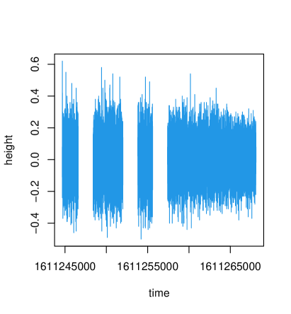
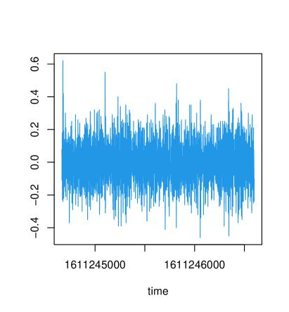
Figure 1: Left panel: representation of the studied time series for buoy 433. The three observed voids represent unobserved data. Right panel: representation of the first segment of the time series in the left panel. Height in meters and time in seconds UTC.

Table 1: The 66 available buoys are labelled by an identification number in descending order. Below it is the length of the associated time series, the smallest being highlighted in bold. The studied label represents the length of the studied time series after selecting the first 30,000 time points and eliminating the unobserved values.

buoy	433	430	256	249	248	244
length	6177194	67207849	55277737	31615487	22526378	81372840
studied	23088	18480	20736	30000	23856	-
buoy	243	240	239	238	236	233
length	29399210	83692847	28618154	2511530	13805738	11474317
studied	3184	23088	2304	4608	7082	22272
buoy	230	226	224	222	221	220
length	36864	52940543	47333545	28634282	6659328	35495593
studied	27696	25392	25392	30000	27696	27696
buoy	217	215	214	213	209	203
length	20561066	22436522	79286411	15161190	18012842	10925950
studied	20614	30000	27696	27696	30000	27696
buoy	201	200	198	197	196	192
length	40785577	7713962	25192106	2520576	80495016	33623807
studied	30000	23855	16006	-	11520	30000
buoy	191	189	187	185	181	179
length	31265450	35170729	39129001	8953514	80459761	58130089
studied	27696	-	11690	27696	27696	25222
buoy	171	168	162	160	158	157
length	42015913	14455296	41025193	854954	97940734	53277865
studied	23856	27696	20784	27696	27696	20614
buoy	155	154	153	150	147	144
length	4737194	32389802	7939754	62576809	55812265	18123434
studied	18480	27696	19968	30000	23088	25514
buoy	143	142	139	134	132	121
length	27956906	16902314	43386793	37933225	39679657	859392
studied	30000	3072	20784	25392	13104	23088
buoy	106	100	098	094	092	076
length	65280	30917546	7206912	12358826	40140457	44669119
studied	9613	27696	7082	23088	-	27696
buoy	071	067	045	036	029	028
length	78400512	32256	990890	141312	9384362	17022122
studied	23088	18480	25392	30000	30000	25344

In the left panel of Figure 1, it is displayed the studied data for buoy 433. As explained when commenting on Table 1, this dataset results from restricting the 6,177,194 observations stored for buoy 433 and taking the ones corresponding to the first 30,000 time points. As it is obvious from the plot, the first 30,000 time points contain unobserved elements. Indeed, only 23,088 observations have been made (see Table 1). From the left panel of the figure, it is also observable that the unobserved data splits the time series in four parts. The right panel of Figure 1 is a zoom of the left panel containing solely the part to the left of the time serie. Coordinated universal times (UTC) in seconds are used for the two panels in the figure. The studied measurements of buoy 433 started being measured at time 1,611,244,667 (see Table 2), which is

Thursday 21st of January of 2021 at the 15:00 hours 57 minutes and 47 seconds

in Greenwich mean time (GMT). The last studied measurement of that buoy was recorded at 1,611,268,104, which is later the same day, at the

22:00 hours 28 minutes and 24 seconds

in GMT. In the x-axis of the plots in the figure, it appears four time points that have been translated in Table 3.

Table 2: For each of the 62 studied buoys, display of the starting and ending time points in seconds UTC of the recordings. The smallest and largest time points are highlighted in bold.

buoy	start time	end time	buoy	start time	end time
	seconds UTC	seconds UTC		seconds UTC	seconds UTC
433	1611244667	1611268104	181	1597067867	1561681704
430	1617209867	1617233304	179	1600117067	1622597437
256	1624062470	1624074188	171	1606739270	1604873585
249	1623769067	1623792504	168	1561658267	1618540104
248	1616997470	1617009188	162	1622574000	1592702904
243	1589644667	1593206904	160	1604861867	1616030738
240	1593183467	1614911304	158	1618516667	1610494104
239	1614887867	1606923037	157	1592679467	1609976867
238	1606899600	1571545704	155	1616007301	1562624904
236	1571522267	1612387707	154	1610470667	1607038104
233	1612364270	1623883518	153	1609953430	1608491585
230	1623871800	1593566904	150	1562601467	1596835704
226	1593543467	1594931304	147	1607014667	1620458907
224	1594907867	1589239704	144	1608479867	1602196104
222	1589216267	1611361704	143	1596812267	1587587304
221	1611338267	1602725304	142	1620435470	1600216988
220	1602701867	1610407704	139	1602172667	1624302037
217	1610384267	1580963304	134	1587563867	1615602504
215	1580939867	1575678504	132	1600205270	1613769185
214	1575655067	1618363704	121	1624278600	1622604504
213	1618340267	1599262104	106	1615579067	1602210504
209	1599238667	1620865704	100	1613757467	1601598504
203	1620842267	1582943304	098	1622581067	1560994104
201	1582919867	1581073107	094	1602187067	1606966104
200	1581049670	1623885185	076	1601575067	1581380904
198	1623873467	1608373837	071	1560970667	1572060504
196	1608350400	1579152504	067	1606942667	1619742504
192	1591718267	1610760504	045	1599843600	1611268104
191	1579129067	1587371304	036	1581357467	1617233304
187	1610737067	1600140504	029	1572037067	1624085907
185	1587347867	1606762707	028	1619719067	1623792504

Table 3: Translation of UTC time points in seconds to regular nomenclature in GMT.

seconds UTC	GMT
1611245000	Thursday January 21st 2021 $16:03:20$
1611246000	Thursday January 21st 2021 $16:20:00$
1611255000	Thursday January 21st 2021 $18:50:00$
1611265000	Thursday January 21st 2021 $21:36:40$

Apart from the ones of station 433, Table 2 displays the starting and ending recording times for each of the studied stations. The largest time value is 1,624,302,037, representing the

Monday 21st of June 2021 at the 19:00 hours and 37 seconds GMT.

This is highlighted in bold in the table. This is the end time for the recording of buoy 139, whose starting time is 1,602,172,667, i.e., the

Thursday 8th of October 2020 at the 15:00 hours 57 minutes and 47 seconds GMT.

Meanwhile, the smallest starting time point is 1,560,970,667, which represents the

Wednesday 19th of June 2019 at the 18:00 hours 57 minutes and 47seconds GMT;

and which is also highlighted in bold in the table. It corresponds to the buoy with identification number 071, whose end time point is 1,572,060,504, i.e. the

Saturday 26th of October 2019 at the 03:00 hours 28 minutes and 24 seconds GMT.

3 Methodology

Given $X_{t}$ a real valued random variable for each $t\in\mathbb{Z},$

$$X:=\{X_{t}\}_{t\in\mathbb{Z}}$$

is a stochastic process Coleman (1974). Most common hypotheses on stochastic processes are those of stationarity Rozanov (1967) and Gaussianity Kozachenko et al. (2016). $X$ is stationary if

• $\mbox{E}[X_{t}]=\mbox{E}[X_{t+k}]$ for all $k,{t}\in\mathbb{Z},$ where E denotes the expectation function,

• $\mbox{Cov}(X_{t},X_{k})=\mbox{Cov}(X_{t-k},X_{0})$ for all $k,{t}\in\mathbb{Z},$ where Cov denotes the covariance function and

• $\mbox{Var}[X_{t}]<\infty$ for all ${t}\in\mathbb{Z},$ where Var denotes the variance.

$X$ is Gaussian if

$$(X_{t_{1}},\ldots,X_{t_{n}})\mbox{ is a Gaussian random vector for all }n\in\mathbb{N}.$$

It occurs that a stationary Gaussian process is strictly stationarity. $X$ is strictly stationary if

$$(X_{t_{1}},\ldots,X_{t_{n}})\mbox{ and }(X_{t_{1+k}},\ldots,X_{t_{n+k}})$$

are equally distributed for all $n\in\mathbb{N}$ and $k,{t_{1}},\ldots,{t_{n}}\in\mathbb{Z}.$ Consequently, given a stationary process $X,$ it is Gaussian if

$$(X_{t},\ldots,X_{t})\mbox{ is a Gaussian random vector for all }t\in\mathbb{N}.$$ (1)

3.1 Tests for stationarity

This manuscript is about testing the Guassianity of stocastic processes. Typically, those tests assume that the process is stationary. Thus, this assumption has to be previously checked. For that, the most common tests in the literature are

1. Ljung-Box test (Box and Pierce, 1970),

2. Augmented Dickey-Fuller test (Said and Dickey, 1984),

3. Phillips-Perron test (Perron, 1988) and

4. kpps test (Kwiatkowski et al., 1992) .

For the first three tests, the tests can be simplified as contrasting the null hypothesis

$$H_{0,1}:X\mbox{ is non stationary}$$ (2)

against the alternative

$$H_{a,1}:X\mbox{ is stationary}$$

while the kpps test results in the null hypothesis

$$H_{0,2}:X\mbox{ is stationary}$$ (3)

against the alternative

$$H_{a,2}:X\mbox{ is non stationary}.$$

The hypotheses are tested in different ways. For instance, Ljung-Box test makes use of the autocorrelation function, which, at lag $k$ for a stationary process is

$$\frac{\mbox{Cov}(X_{t},X_{t+k})}{\mbox{Var}(X_{t})}.$$

This is observable from its statistic:

$$n(n+2)\sum_{k=1}^{h}\frac{\hat{\rho}^{2}_{k}}{n-k},$$

where $\hat{\rho}_{k}$ denotes the sample autocorrelation at lag $k$ and $n$ the sample size. Note that it depends on a constant $h.$

3.2 Tests for Gaussianity

Most tests for Gaussianity of stochastic processes assume the process is stationary and test whether a finite marginal distribution of the process is Gaussian, generally, the one-dimensional marginal. That is, instead of testing whether (1) is satisfied, these tests contrast the null hypothesis

$$H_{0,3}:X_{t}\mbox{ is a Gaussian random variable}$$ (4)

against the alternative

$$H_{a,3}:X_{t}\mbox{ is not a Gaussian random variable}$$

by checking whether $X_{t}$ is a Gaussian random variable. Let us reflect that, because of the stationarity, the distribution of $X_{t}$ is the same for all $t\in\mathbb{Z};$ that is, it is independent of $t.$

Common tests to check the Gaussianity of a real valued random variable require a sample of independent and identically distributed random variables D’Agostino and Stephens (1986). As this work deals with stochastic processes, the independence assumption is not verified. However, there are also many tests for this situation. Here, it is made use of the Epps test Epps (1987), which checks that the characteristic function of the one-dimensional distribution of the process is that of a Gaussian distribution, and of the Lobato and Velasco test Lobato and Velasco (2004), which checks that the third and fourth order moments of the one-dimensional distribution of the process are those of a Gaussian distribution.

If the null hypothesis $H_{0,3}$ is rejected, with the above mentioned tests, the null hypothesis

$$H_{0,4}:X\mbox{ is a Gaussian process}$$ (5)

is rejected against the alternative

$$H_{a,4}:X\mbox{ is not a Gaussian process}.$$

However, it may occur that

$$X_{t}\mbox{ is a Gaussian random variable}$$

while

$$X\mbox{ is not a Gaussian process}.$$

The above mentioned tests are at nominal level again this type of alternatives. For this, it is used here the random projection test Nieto-Reyes, Cuesta-Albertos and Gamboa (2014), which test the Gaussianity of the whole distribution of the process and not just of a finite dimensional marginal. For elaboration on it, see Subsection 3.2.1.

3.2.1 Random projection test

The random projection test was introduced in Nieto-Reyes, Cuesta-Albertos and Gamboa (2014) as a tool to test the Gaussianity of stationary processes that is able to reject the null hypothesis of Gaussianity (5) against alternatives with Gaussian finite-dimensional marginals. The procedure is based on a result in Cuesta-Albertos et al. (2007) that implies that if

$$\langle\{X_{j}\}_{j\leq t},d\rangle,$$

with $d$ drawn from a Dirichlet distribution J. (2006), is Gaussian, then

$$\{X_{j}\}_{j\leq t}$$

is Gaussian. Note that due to the stationarity assumption, the Gaussianity of $\{X_{j}\}_{j\leq t}$ is equivalent to (1). In what follows, the procedure is explained in detail.

Let

$$\lambda_{1},\lambda_{2}>0$$

be two parameters. Making use of the following stick-breaking procedure, a Dirichlet distribution is considered:

1. Let

   $$\beta(\lambda_{1},\lambda_{2})$$

   denote a beta distribution with parameters $\lambda_{1},\lambda_{2}.$

2. Let $d_{0}$ be drawn from the distribution $\beta(\lambda_{1},\lambda_{2}).$ Note that

   $$d_{0}\in[0,1].$$

3. For any $k\in\mathbb{N},$ the natural numbers, let $d_{k}$ be the result of multiplying

   $$1-\sum_{i=0}^{k-1}d_{i}$$

   and an element drawn independently from he distribution $\beta(\lambda_{1},\lambda_{2}).$ Note that

   $$d_{k}\in[0,1-\sum_{i=0}^{k-1}d_{i}].$$

Let $X$ be a stationary process. The associated projected process based on $\{d_{k}\}_{k\in\mathbb{N}}$ is

$$Y:=\{Y_{t}\}_{t\in\mathbb{Z}}$$

with

$$Y_{t}:=\sum_{i=0}^{\infty}d_{i}X_{t-i}.$$

Then, making use of this randomly projected process, it suffices to apply to it a test for the null hypothesis of Gaussianity (4).

The selection of the parameters $\lambda_{1},\lambda_{2}$ is important. It is explained in Nieto-Reyes, Cuesta-Albertos and Gamboa (2014) that values such us

$$\lambda_{1}=100\mbox{ and }\lambda_{2}=1$$

result in an projected process $Y$ similar to $X.$ However, values such us

$$\lambda_{1}=2\mbox{ and }\lambda_{2}=7$$

result in projected processes different from $X$ while providing an effective method.

3.3 False discovery rate

When multiple tests are perform, the multiplicity has to be taken into account. For that it is used here the false discovery rate (Benjamini and Yekutieli, 2001). The false discovery rate aims at controling the expected proportion of falsely rejected hypothesis. It was first introduced in Benjamini and Hochberg (1995) to take into account the multiplicity of independent tests. In (Benjamini and Yekutieli, 2001) it was established that the definition in (Benjamini and Hochberg, 1995) remains valid for certain types of dependency. However, for general dependent cases (Benjamini and Yekutieli, 2001) has to be applied.

4 Results of the analysis

This section analyzes whether each of the 62 datasets provided in Section 2, one per buoy, is drawn from a Gaussian process. For that, the tests described in Section 3.2 are used here. As they require the stationarity assumption for the process, making use of the tests provided in 3.1, it is first checked whether each of the datasets is drawn from a stationary process.

The results obtained from checking the stationarity are displayed in Table 4. Only one result is provided by test because the same one is obtained for each of the 62 datasets. Thus, p-values smaller than .01 are obtained for the Augmented Dickey-Fuller test and the Phillips-Perron test. P-values that are approximately zero are obtained for the Ljung-Box test and p-values larger than .1 for the kpps test. Note that in the first three tests the null hypothesis of non-stationarity is tested, as in (2), and in the fourth it is the null hypothesis of stationarity, as in (3). Thus, it can be assumed that the studied datasets are drawn from stationary processes, and check their Gaussianity under the mentioned assumption.

Table 4: Obtained p-values for each of the 62 studied datasets under four different stationarity tests: Augmented Dickey-Fuller (first column), Phillips-Perron (second column), Ljung-Box test (third column) and kpps (fourth column). The null hypothesis is of stationarity for the kpps test and of non-stationarity for the other three.

		Tests
	Augmented Dickey-Fuller	Phillips-Perron	Ljung-Box	kpps
p-value	$<.01$	$<.01$	0	$>.1$

In order to study the Gaussianity of the datasets under study, it is first analyzed the one-dimensional marginal distribution of the process. This is because a rejection of the null hypothesis (4) implies the sought rejection of the whole distribution of the process, in (5). For analyzing the one-dimensional marginal distribution, it is made use of the Epps and Lobato and Velasco tests commented in Section 3. The results are displayed in Table 5. There, for each dataset, associated to a buoy (columns 1 and 5), it can be observed the p-values resulting from applying the Epps test (columns 2 and 6) and the Lobato and Velasco test (columns 3 and 7). As multiplicity has to be taken into account, columns 4 and 8 display the FDR values. It can be observed from the table that half of the 62 FDR values are smaller than 0.05 studied. They have been highlighted in bold. If the less conservative FDR introduced in (Benjamini and Hochberg, 1995) had been used, the number of rejections would have increased. For instance, the null hypothesis (4) for buoys 185 and 028 would also have been rejected. If multiplicity had not been taken into account at all and the null hypothesis (4) were rejected when the minimum of the two p-values was smaller than 0.05, the number of rejections would have increased to 40.

Table 5: P-values resulting from applying the Epps test (columns 2 and 6) and the Lobato and Velasco test (columns 3 and 7) per dataset associated to each buoy (columns 1 and 5). FDR (columns 4 and 8) combination, for dependent p-values, of the two p-values per buoy, with the ones smaller than 0.05 highlighted in bold.

buoy	Epps	L.-V.	FDR	buoy	Epps	L.-V.	FDR
433	.000	.000	.000	181	.000	.000	.000
430	.027	.000	.000	179	.000	.000	.000
256	.004	.000	.000	171	.000	.000	.000
249	.000	.000	.000	168	.001	.000	.000
248	.524	.044	.132	162	.331	.046	.138
243	.063	.044	.095	160	.111	.011	.033
240	.017	.000	.000	158	.290	.178	.436
239	.297	.780	.891	157	.116	.599	.349
238	.000	.552	1.656	155	.066	.063	.099
236	.708	.142	.426	154	.011	.000	.000
233	.004	.000	.000	153	.028	.000	.000
230	.000	.000	.000	150	.013	.000	.000
226	.254	.030	.090	147	.055	.001	.003
224	.000	.000	.000	144	.000	.000	.000
222	.821	.788	1.231	143	.261	.005	.015
221	.000	.000	.000	142	.586	.093	.279
220	.739	.356	1.068	139	.292	.646	.877
217	.000	.000	.000	134	.188	.000	.000
215	.057	.035	.086	132	.017	.000	.000
214	.068	.004	.012	121	.001	.000	.000
213	.002	.001	.003	106	.574	.887	1.4330
209	.817	.000	.000	100	.122	.114	.183
203	.948	.857	1.422	098	.280	.914	.840
201	.329	.227	.493	094	.521	.056	.168
200	.000	.000	.000	076	.068	.110	.165
198	.090	.000	.000	071	.261	.020	.060
196	.235	.062	.186	067	.790	.426	1.184
192	.093	.000	.000	045	.587	.222	.666
191	.535	.079	.237	036	.002	.011	.007
187	.803	.334	1.002	029	.472	.990	1.416
185	.020	.287	.059	028	.359	.017	.051

To better illustrate the findings, the results of Table 5 are summarized in the left plot of Figure 2. The $x$-axis represents the buoy’s identification number while the $y$-axis displays the obtained FDR for dependent tests. A grey line at $y=0.05$ is drawn to show what buoys have a FDR above or below that value, which result in a rejection of the null hypothesis (4). It can observe that there are three FDR that are just above 0.05. They correspond to buoys 028, 071 and 185.

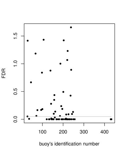
Figure 2: Left panel: FDR corresponding to the studied buoys in Table 5. Right panel: P-value corresponding to the buoys studied in Table 6. P-values obtained with the random projection test based on the one-dimensional Lovato and Velasco test are represented in color blue and those based on the Epps test are in color green. The line $y=.05$ is displayed in both panels in color grey.

Table 6: P-values (column 2) resulting of applying the random projection test for each buoy (column 1) with a FDR adjusted p-value larger than 0.05 in Table 5. The parameters (columns 3 and 4) and the one-dimensional test (column 5) used in performing the random projection test are included for each buoy.

buoy	p-value	param1	param2	test
248	.017	100	1	L.-V.
243	.044	100	1	L.-V.
239	.362	100	1	Epps
238	.000	100	1	Epps
236	.055	2	7	L.-V.
226	.040	100	1	L.-V.
222	.048	2	7	L.-V.
220	.411	2	7	Epps
215	.050	100	1	L.-V.
203	.340	2	7	Epps
201	.020	100	1	L.-V.
196	.017	2	7	L.-V.
191	.020	100	1	L.-V.
187	.039	2	7	L.-V.
185	.017	100	1	Epps
162	.042	100	1	L.-V.
158	.476	2	7	Epps
157	.456	2	7	Epps
155	.024	100	1	L.-V.
142	.021	100	1	L.-V.
139	.376	2	7	Epps
106	.374	2	7	Epps
100	.412	100	1	Epps
098	.416	100	1	Epps
094	.027	100	1	L.-V.
076	.398	100	1	Epps
071	.021	100	1	L.-V.
067	.019	100	1	L.-V.
045	.022	100	1	L.-V.
029	.381	100	1	Epps
028	.028	100	1	L.-V.

In what follows it is pursued a further study in the 31 buoys for which there is yet no evidence to reject the null hypothesis of Gaussianity, displayed in (5). This further study consists in applying the random projection test. In applying it, the information in Table 5 obtained when applying de Epps and Lobato and Velasco tests is used. For instance, if for one of these two tests the associated p-value is smaller than 0.05, it is made use of that test and the parameters $(100,1)$ in computing the random projection test. Remember that, as commented in Section 3, making use of the $(100,1)$ parameters results in a projected time series similar to the original one.

The results of applying the random projection test are reported in Table 6. There it can be observed that the random projection test is able to reject the null hypothesis of Gaussianity in 19 out of the 31 buoys, which results in a total of 50 rejections out of 62 (the 80.65$\%$). The p-values that result in a rejection are highlighted in bold. The p-value associated to buoy 215 has been highlighted because it takes value 4.966946e-02, which in the table has been rounded to 0.050. The table also provides the parameters used to compute the projection and the test applied to it.

The results in Table 6 have been summarized in the right plot of Figure 2. There, the p-values larger and smaller than 0.05 can be clearly observed; and that there is a p-value just above 0.05, the one corresponding to buoy 236. The p-values where the Lovato and Velasco test is used in performing the random projection test are colored in blue. Those in which the random projection test makes use of the Epps test are colored in green.

References

- Azaïs, León and Ortega (2005) {barticle}[author] \bauthor\bsnmAzaïs, \bfnmJean-Marc\binitsJ.-M., \bauthor\bsnmLeón, \bfnmJosé R.\binitsJ. R. and \bauthor\bsnmOrtega, \bfnmJoaquín\binitsJ. (\byear2005). \btitleGeometrical characteristics of Gaussian sea waves. \bjournalJournal of Applied Probability \bvolume42 \bpages407–425. \bdoi10.1239/jap/1118777179 \endbibitem
- Battjes and Groenendijk (2000) {barticle}[author] \bauthor\bsnmBattjes, \bfnmJurjen A\binitsJ. A. and \bauthor\bsnmGroenendijk, \bfnmHeiko W\binitsH. W. (\byear2000). \btitleWave height distributions on shallow foreshores. \bjournalCoastal Engineering \bvolume40 \bpages161-182. \bdoihttps://doi.org/10.1016/S0378-3839(00)00007-7 \endbibitem
- Benetazzo et al. (2015) {barticle}[author] \bauthor\bsnmBenetazzo, \bfnmA.\binitsA., \bauthor\bsnmBarbariol, \bfnmF.\binitsF., \bauthor\bsnmBergamasco, \bfnmF.\binitsF., \bauthor\bsnmTorsello, \bfnmA.\binitsA., \bauthor\bsnmCarniel, \bfnmS.\binitsS. and \bauthor\bsnmSclavo, \bfnmM\binitsM. (\byear2015). \btitleObservation of Extreme Sea Waves in a Space–Time Ensemble. \bjournalJournal of Physical Oceanography \bvolume45 \bpages2261-2275. \endbibitem
- Benjamini and Hochberg (1995) {barticle}[author] \bauthor\bsnmBenjamini, \bfnmYoav\binitsY. and \bauthor\bsnmHochberg, \bfnmYosef\binitsY. (\byear1995). \btitleControlling the False Discovery Rate: A Practical and Powerful Approach to Multiple Testing. \bjournalJournal of the Royal Statistical Society. Series B (Methodological) \bvolume57 \bpages289–300. \endbibitem
- Benjamini and Yekutieli (2001) {barticle}[author] \bauthor\bsnmBenjamini, \bfnmYoav\binitsY. and \bauthor\bsnmYekutieli, \bfnmDaniel\binitsD. (\byear2001). \btitleThe Control of the False Discovery Rate in Multiple Testing under Dependency. \bjournalThe Annals of Statistics \bvolume29 \bpages1165–1188. \endbibitem
- Boccotti (1989) {barticle}[author] \bauthor\bsnmBoccotti, \bfnmP.\binitsP. (\byear1989). \btitleOn Mechanics of Irregular Gravity Waves. \bjournalAtti della Accademia Nazionale dei Lincei, Memorie \bvolume19 \bpages110-170. \endbibitem
- Box and Pierce (1970) {barticle}[author] \bauthor\bsnmBox, \bfnmG. E. P.\binitsG. E. P. and \bauthor\bsnmPierce, \bfnmDavid A.\binitsD. A. (\byear1970). \btitleDistribution of Residual Autocorrelations in Autoregressive-Integrated Moving Average Time Series Models. \bjournalJournal of the American Statistical Association \bvolume65 \bpages1509-1526. \bdoi10.1080/01621459.1970.10481180 \endbibitem
- Casas‐Prat and Holthuijsen (2010) {barticle}[author] \bauthor\bsnmCasas‐Prat, \bfnmM.\binitsM. and \bauthor\bsnmHolthuijsen, \bfnmL. H.\binitsL. H. (\byear2010). \btitleShort‐term statistics of waves observed in deep water. \bjournalJournal of Geophysical Research: Oceans \bvolume115 (C9). \bdoihttps://doi.org/10.1029/2009JC005742 \endbibitem
- Coleman (1974) {binbook}[author] \bauthor\bsnmColeman, \bfnmRodney\binitsR. (\byear1974). \btitleWhat is a Stochastic Process? In \bbooktitleStochastic Processes \bpages1–5. \bpublisherSpringer Netherlands, \baddressDordrecht. \bdoi10.1007/978-94-010-9796-3_1 \endbibitem
- Collins et al. (2014) {barticle}[author] \bauthor\bsnmCollins, \bfnmClarence O\binitsC. O., \bauthor\bsnmLund, \bfnmBjörn\binitsB., \bauthor\bsnmWaseda, \bfnmTakuji\binitsT. and \bauthor\bsnmGraber, \bfnmHans C\binitsH. C. (\byear2014). \btitleOn recording sea surface elevation with accelerometer buoys: lessons from ITOP (2010). \bjournalOcean dynamics \bvolume64 \bpages895–904. \endbibitem
- Cuesta-Albertos et al. (2007) {barticle}[author] \bauthor\bsnmCuesta-Albertos, \bfnmJ. A.\binitsJ. A., \bauthor\bparticledel \bsnmBarrio, \bfnmE.\binitsE., \bauthor\bsnmFraiman, \bfnmR.\binitsR. and \bauthor\bsnmMatrán, \bfnmC.\binitsC. (\byear2007). \btitleThe Random Projection Method in Goodness of Fit for Functional Data. \bjournalComputational Statistics & Data Analysis \bvolume51 \bpages4814 - 4831. \bdoihttps://doi.org/10.1016/j.csda.2006.09.007 \endbibitem
- D’Agostino and Stephens (1986) {barticle}[author] \bauthor\bsnmD’Agostino, \bfnmRalph B.\binitsR. B. and \bauthor\bsnmStephens, \bfnmMichael A.\binitsM. A. (\byear1986). \btitleGoodness-of-fit techniques. \bjournalQuality and Reliability Engineering International \bvolume3 \bpages71-71. \bdoi10.1002/qre.4680030121 \endbibitem
- Epps (1987) {barticle}[author] \bauthor\bsnmEpps, \bfnmT. W.\binitsT. W. (\byear1987). \btitleTesting That a Stationary Time Series is Gaussian. \bjournalThe Annals of Statistics \bvolume15 \bpages1683–1698. \bdoi10.1214/aos/1176350618 \endbibitem
- Forristall (1978) {barticle}[author] \bauthor\bsnmForristall, \bfnmG. Z.\binitsG. Z. (\byear1978). \btitleOn the statistical distribution of wave heights in a storm. \bjournalJournal of Geophysical Research: Oceans \bvolume83 \bpages2353-2358. \endbibitem
- Haver (1987) {barticle}[author] \bauthor\bsnmHaver, \bfnmSverre\binitsS. (\byear1987). \btitleOn the joint distribution of heights and periods of sea waves. \bjournalOcean Engineering \bvolume14 \bpages359-376. \bdoihttps://doi.org/10.1016/0029-8018(87)90050-3 \endbibitem
- Hessner, Reichert and Hutt (2007) {binproceedings}[author] \bauthor\bsnmHessner, \bfnmKatrin\binitsK., \bauthor\bsnmReichert, \bfnmKonstanze\binitsK. and \bauthor\bsnmHutt, \bfnmBelmont-Lower\binitsB.-L. (\byear2007). \btitleSea surface elevation maps obtained with a nautical X-Band radar–Examples from WaMoS II stations. In \bbooktitle10th International Workshop on Wave Hindcasting and Forecasting and Coastal Hazard Symposium, North Shore, Oahu, Hawaii \bpages11–16. \endbibitem
- Hokimoto and Shimizu (2014) {barticle}[author] \bauthor\bsnmHokimoto, \bfnmTsukasa\binitsT. and \bauthor\bsnmShimizu, \bfnmKunio\binitsK. (\byear2014). \btitleA non-homogeneous hidden Markov model for predicting the distribution of sea surface elevation. \bjournalJournal of applied statistics \bvolume41 \bpages294–319. \endbibitem
- J. (2006) {bincollection}[author] \bauthor\bsnmJ., \bfnmPitman\binitsP. (\byear2006). \btitleCombinatorial Stochastic Processes. In \bbooktitleLectures from the 32nd Summer School on Probability Theory held in Saint-Flour \bpublisherSpringer. \endbibitem
- Jishad, Yadhunath and Seelam (2021) {barticle}[author] \bauthor\bsnmJishad, \bfnmM.\binitsM., \bauthor\bsnmYadhunath, \bfnmE. M.\binitsE. M. and \bauthor\bsnmSeelam, \bfnmJaya Kumar\binitsJ. K. (\byear2021). \btitleWave height distribution in unsaturated surf zones. \bjournalRegional Studies in Marine Science \bvolume44 \bpages101708. \bdoihttps://doi.org/10.1016/j.rsma.2021.101708 \endbibitem
- Karmpadakis, Swan and Christou (2020) {barticle}[author] \bauthor\bsnmKarmpadakis, \bfnmI.\binitsI., \bauthor\bsnmSwan, \bfnmC.\binitsC. and \bauthor\bsnmChristou, \bfnmM.\binitsM. (\byear2020). \btitleAssessment of wave height distributions using an extensive field database. \bjournalCoastal Engineering \bvolume157 \bpages103630. \bdoihttps://doi.org/10.1016/j.coastaleng.2019.103630 \endbibitem
- Klopman (1996) {barticle}[author] \bauthor\bsnmKlopman, \bfnmG.\binitsG. (\byear1996). \btitleExtreme wave heights in shallow water. \bjournalWL—Delft Hydraulics \bvolumeReport H2486. \endbibitem
- Kozachenko et al. (2016) {bincollection}[author] \bauthor\bsnmKozachenko, \bfnmYuriy\binitsY., \bauthor\bsnmPogorilyak, \bfnmOleksandr\binitsO., \bauthor\bsnmRozora, \bfnmIryna\binitsI. and \bauthor\bsnmTegza, \bfnmAntonina\binitsA. (\byear2016). \btitle2 - Simulation of Stochastic Processes Presented in the Form of Series. In \bbooktitleSimulation of Stochastic Processes with Given Accuracy and Reliability (\beditor\bfnmYuriy\binitsY. \bsnmKozachenko, \beditor\bfnmOleksandr\binitsO. \bsnmPogorilyak, \beditor\bfnmIryna\binitsI. \bsnmRozora and \beditor\bfnmAntonina\binitsA. \bsnmTegza, eds.) \bpages71-104. \bpublisherElsevier. \bdoihttps://doi.org/10.1016/B978-1-78548-217-5.50002-7 \endbibitem
- Kwiatkowski et al. (1992) {barticle}[author] \bauthor\bsnmKwiatkowski, \bfnmDenis\binitsD., \bauthor\bsnmPhillips, \bfnmPeter C. B.\binitsP. C. B., \bauthor\bsnmSchmidt, \bfnmPeter\binitsP. and \bauthor\bsnmShin, \bfnmYongcheol\binitsY. (\byear1992). \btitleTesting the Null Hypothesis of Stationarity Against the Alternative of a Unit Root: How sure Are We that Economic Time Series Have a Unit Root? \bjournalJournal of Econometrics \bvolume54 \bpages159 - 178. \bdoihttps://doi.org/10.1016/0304-4076(92)90104-Y \endbibitem
- Lobato and Velasco (2004) {barticle}[author] \bauthor\bsnmLobato, \bfnmIgnacio\binitsI. and \bauthor\bsnmVelasco, \bfnmCarlos\binitsC. (\byear2004). \btitleA simple Test of Normality for Time Series. \bjournalEconometric Theory \bvolume20 \bpages671-689. \bdoi10.1017/S0266466604204030 \endbibitem
- Longuet-Higgins (1980) {barticle}[author] \bauthor\bsnmLonguet-Higgins, \bfnmMichael S.\binitsM. S. (\byear1980). \btitleOn the distribution of the heights of sea waves: Some effects of nonlinearity and finite band width. \bjournalJournal of Geophysical Research: Oceans \bvolume85 \bpages1519-1523. \bdoihttps://doi.org/10.1029/JC085iC03p01519 \endbibitem
- Mendes and Scotti (2021) {barticle}[author] \bauthor\bsnmMendes, \bfnmS.\binitsS. and \bauthor\bsnmScotti, \bfnmA.\binitsA. (\byear2021). \btitleThe Rayleigh-Haring-Tayfun distribution of wave heights in deep water. \bjournalApplied Ocean Research \bvolume113 \bpages102739. \bdoihttps://doi.org/10.1016/j.apor.2021.102739 \endbibitem
- Mendez, Losada and Medina (2004) {barticle}[author] \bauthor\bsnmMendez, \bfnmFernando J\binitsF. J., \bauthor\bsnmLosada, \bfnmInigo J\binitsI. J. and \bauthor\bsnmMedina, \bfnmRaul\binitsR. (\byear2004). \btitleTransformation model of wave height distribution on planar beaches. \bjournalCoastal Engineering \bvolume50 \bpages97-115. \bdoihttps://doi.org/10.1016/j.coastaleng.2003.09.005 \endbibitem
- Mori, Liu and Yasuda (2002) {barticle}[author] \bauthor\bsnmMori, \bfnmNobuhito\binitsN., \bauthor\bsnmLiu, \bfnmPaul C\binitsP. C. and \bauthor\bsnmYasuda, \bfnmTakashi\binitsT. (\byear2002). \btitleAnalysis of freak wave measurements in the Sea of Japan. \bjournalOcean Engineering \bvolume29 \bpages1399-1414. \bdoihttps://doi.org/10.1016/S0029-8018(01)00073-7 \endbibitem
- Muraleedharan et al. (2007) {barticle}[author] \bauthor\bsnmMuraleedharan, \bfnmG.\binitsG., \bauthor\bsnmRao, \bfnmA. D.\binitsA. D., \bauthor\bsnmKurup, \bfnmP. G.\binitsP. G., \bauthor\bsnmNair, \bfnmN. Unnikrishnan\binitsN. U. and \bauthor\bsnmSinha, \bfnmMourani\binitsM. (\byear2007). \btitleModified Weibull distribution for maximum and significant wave height simulation and prediction. \bjournalCoastal Engineering \bvolume54 \bpages630-638. \endbibitem
- Naess (1985) {barticle}[author] \bauthor\bsnmNaess, \bfnmArvid\binitsA. (\byear1985). \btitleOn the distribution of crest to trough wave heights. \bjournalOcean Engineering \bvolume12 \bpages221-234. \bdoihttps://doi.org/10.1016/0029-8018(85)90014-9 \endbibitem
- Nieto-Reyes (2021) {barticle}[author] \bauthor\bsnmNieto-Reyes, \bfnmAlicia\binitsA. (\byear2021). \btitleOn the Non-Gaussianity of the Height of Sea Waves. \bjournalJournal of Marine Science and Engineering \bvolume9. \bdoi10.3390/jmse9121446 \endbibitem
- Nieto-Reyes, Cuesta-Albertos and Gamboa (2014) {barticle}[author] \bauthor\bsnmNieto-Reyes, \bfnmAlicia\binitsA., \bauthor\bsnmCuesta-Albertos, \bfnmJuan Antonio\binitsJ. A. and \bauthor\bsnmGamboa, \bfnmFabrice\binitsF. (\byear2014). \btitleA Random-Projection Based Test of Gaussianity for Stationary Processes. \bjournalComputational Statistics & Data Analysis \bvolume75 \bpages124 - 141. \bdoihttps://doi.org/10.1016/j.csda.2014.01.013 \endbibitem
- Pena-Sanchez, Mérigaud and Ringwood (2018) {barticle}[author] \bauthor\bsnmPena-Sanchez, \bfnmYerai\binitsY., \bauthor\bsnmMérigaud, \bfnmAlexis\binitsA. and \bauthor\bsnmRingwood, \bfnmJohn V\binitsJ. V. (\byear2018). \btitleShort-term forecasting of sea surface elevation for wave energy applications: The autoregressive model revisited. \bjournalIEEE Journal of Oceanic Engineering \bvolume45 \bpages462–471. \endbibitem
- Perron (1988) {barticle}[author] \bauthor\bsnmPerron, \bfnmPierre\binitsP. (\byear1988). \btitleTrends and Random Walks in Macroeconomic Time Series: Further Evidence From a New Approach. \bjournalJournal of Economic Dynamics and Control \bvolume12 \bpages297 - 332. \bdoihttps://doi.org/10.1016/0165-1889(88)90043-7 \endbibitem
- Reichert, Dannenberg and van den Boom (2010) {binproceedings}[author] \bauthor\bsnmReichert, \bfnmKonstanze\binitsK., \bauthor\bsnmDannenberg, \bfnmJens\binitsJ. and \bauthor\bparticlevan den \bsnmBoom, \bfnmHenk\binitsH. (\byear2010). \btitleX-Band radar derived sea surface elevation maps as input to ship motion forecasting. In \bbooktitleOCEANS’10 IEEE SYDNEY \bpages1–7. \bpublisherIEEE. \endbibitem
- Rozanov (1967) {bmisc}[author] \bauthor\bsnmRozanov, \bfnmY. A.\binitsY. A. (\byear1967). \btitleStationary random processes. \bhowpublishedSan Francisco-Cambridge-London-Amsterdam: Holden-Day 1967. 211 p. (1967). \endbibitem
- Said and Dickey (1984) {barticle}[author] \bauthor\bsnmSaid, \bfnmSaid E.\binitsS. E. and \bauthor\bsnmDickey, \bfnmDavid A.\binitsD. A. (\byear1984). \btitleTesting for Unit Roots in Autoregressive-Moving Average Models of Unknown Order. \bjournalBiometrika \bvolume71 \bpages599-607. \bdoi10.1093/biomet/71.3.599 \endbibitem
- Schulz-Stellenfleth and Lehner (2004) {barticle}[author] \bauthor\bsnmSchulz-Stellenfleth, \bfnmJohannes\binitsJ. and \bauthor\bsnmLehner, \bfnmSusanne\binitsS. (\byear2004). \btitleMeasurement of 2-D sea surface elevation fields using complex synthetic aperture radar data. \bjournalIEEE Transactions on Geoscience and Remote Sensing \bvolume42 \bpages1149–1160. \endbibitem
- Srokosz (1986) {barticle}[author] \bauthor\bsnmSrokosz, \bfnmMA\binitsM. (\byear1986). \btitleOn the joint distribution of surface elevation and slopes for a nonlinear random sea, with an application to radar altimetry. \bjournalJournal of Geophysical Research: Oceans \bvolume91 \bpages995–1006. \endbibitem
- Srokosz and Longuet-Higgins (1986) {barticle}[author] \bauthor\bsnmSrokosz, \bfnmMA\binitsM. and \bauthor\bsnmLonguet-Higgins, \bfnmMS\binitsM. (\byear1986). \btitleOn the skewness of sea-surface elevation. \bjournalJournal of Fluid Mechanics \bvolume164 \bpages487–497. \endbibitem
- Stansell (2004) {barticle}[author] \bauthor\bsnmStansell, \bfnmPaul\binitsP. (\byear2004). \btitleDistributions of freak wave heights measured in the North Sea. \bjournalApplied Ocean Research \bvolume26 \bpages35-48. \bdoihttps://doi.org/10.1016/j.apor.2004.01.004 \endbibitem
- Stansell (2005) {barticle}[author] \bauthor\bsnmStansell, \bfnmPaul\binitsP. (\byear2005). \btitleDistributions of extreme wave, crest and trough heights measured in the North Sea. \bjournalOcean Engineering \bvolume32 \bpages1015-1036. \bdoihttps://doi.org/10.1016/j.oceaneng.2004.10.016 \endbibitem
- Tayfun (1990) {barticle}[author] \bauthor\bsnmTayfun, \bfnmM. Aziz\binitsM. A. (\byear1990). \btitleDistribution of Large Wave Heights. \bjournalJournal of Waterway, Port, Coastal, and Ocean Engineering \bvolume116 \bpages686-707. \bdoi10.1061/(ASCE)0733-950X(1990)116:6(686) \endbibitem
- van Vledder (1991) {barticle}[author] \bauthor\bparticlevan \bsnmVledder, \bfnmG. P.\binitsG. P. (\byear1991). \btitleModification of the Glukhovskiy distribution. \bjournalTechnical report, Delft Hydraulics \bvolumeReport H1203. \endbibitem
- Wu et al. (2016) {barticle}[author] \bauthor\bsnmWu, \bfnmYanyun\binitsY., \bauthor\bsnmRandell, \bfnmDavid\binitsD., \bauthor\bsnmChristou, \bfnmMarios\binitsM., \bauthor\bsnmEwans, \bfnmKevin\binitsK. and \bauthor\bsnmJonathan, \bfnmPhilip\binitsP. (\byear2016). \btitleOn the distribution of wave height in shallow water. \bjournalCoastal Engineering \bvolume111 \bpages39-49. \bdoihttps://doi.org/10.1016/j.coastaleng.2016.01.015 \endbibitem