Scalable Polar Code Construction for Successive Cancellation List Decoding:
A Graph Neural Network-Based Approach

Abstract

While constructing polar codes for successive-cancellation decoding can be implemented efficiently by sorting the bit channels, finding optimal polar codes for cyclic-redundancy-check-aided successive-cancellation list (CA-SCL) decoding in an efficient and scalable manner still awaits investigation. This paper first maps a polar code to a unique heterogeneous graph called the polar-code-construction message-passing (PCCMP) graph. Next, a heterogeneous graph-neural-network-based iterative message-passing (IMP) algorithm is proposed which aims to find a PCCMP graph that corresponds to the polar code with minimum frame error rate under CA-SCL decoding. This new IMP algorithm’s major advantage lies in its scalability power. That is, the model complexity is independent of the blocklength and code rate, and a trained IMP model over a short polar code can be readily applied to a long polar code’s construction. Numerical experiments show that IMP-based polar-code constructions outperform classical constructions under CA-SCL decoding. In addition, when an IMP model trained on a length-$128$ polar code directly applies to the construction of polar codes with different code rates and blocklengths, simulations show that these polar-code constructions deliver comparable performance to the 5G polar codes.

I Introduction

Polar codes, originally introduced by Arıkan in [1], have attracted wide interest from both academia and industry because of their capacity-achieving property for a binary-input memoryless symmetric channel under the successive-cancellation (SC) decoding. Despite being asymptotically capacity-achieving, polar codes’ performance with SC decoding is unsatisfactory for short blocklengths. The performance is improved in [2] by concatenating the polar code with a cyclic redundancy check (CRC) code and adopting CRC-aided SC list (CA-SCL) decoding, yet is still far from the random-coding union bound [3]. Recently, Arıkan improves his polar codes through the polarization-adjusted convolutional (PAC) code that closely approaches the dispersion bound of the binary-input additive white Gaussian noise (AWGN) channel under serial decoding and list decoding [4, 5]. The 5G standard uses polar codes in the control channel, where short blocklength codes are required [6].

The polar-encoding process divides the source vector into two parts, the non-frozen bits and the frozen bits. The non-frozen bits correspond to the message, while the frozen bits are predefined values known to the decoder. The transmitter encodes source vector with the polar transformation matrix to produce a polar codeword. Polar-code construction designs the frozen set under a given channel condition and for a given decoding algorithm to minimize the frame error rate (FER).

Recent research proposes multiple techniques to construct polar codes tailored for the SC decoding. Some important examples include the use of the Bhattacharyya parameter and its variants [1, 7], methods based on density evolution [8, 9], Gaussian approximation of density evolution [10], channel upgrading/downgrading techniques [11] for general symmetric binary-input memoryless channels, and a Monte-Carlo-based bit-channel selection algorithm that handles general channel conditions [12]. Recent works [13, 14] introduce a universal partial ordering of bit-channel reliability that leads to a polar-code construction algorithm whose complexity is sublinear in blocklength [15]. He et al. propose a $\beta$-expansion construction method based on this universal partial order in [16].

All aforementioned construction techniques rely on the premise that the information bits should be transmitted over the most reliable bit-channels to achieve the optimal error-correction performance with SC decoding. However, experiments show that with SC list (SCL) or CA-SCL decoding, the polar codes based upon the most reliable bit-channels’ selection do not necessarily result in the best error-correction performance [17]. With SCL decoding, there may not even exist a single reliability order of bit-channels that optimizes polar-code constructions for arbitrary code rates. Nevertheless, the current 5G NR standard polar-code design uses a universal reliability order of $1024$ bit-channels [18]. The composition of such a universal reliability order accounts for the partial reliability order imposed by the polarization effect on bit-channels [15], the distance properties [17], and the list-decoder use. For a given channel, rigorous performance analysis for the optimal code construction under SCL decoding still remains an open problem. However, some important theoretical breakthroughs advance polar codes’ understanding: [19] characterizes the polar code’s minimum distance, and [13] recognizes polar codes as decreasing monomial codes. In [20], Yao et al. developed a deterministic recursive algorithm that computes the polar codes’ weight enumerating function. Recently, Coşkun and Pfister [21] analyzed the SCL decoder’s required list size to approach the maximum-likelihood decoding performance. Several methods, including parity-check designs [22, 23], dynamic frozen bits design [24, 25], weight-distribution optimization [26, 27, 28, 29, 30] and altering construction patterns [31, 32, 33] improve polar codes’ design for SCL decoding. The authors of [31] propose a log-likelihood ratio (LLR)-evolution-based construction method that swaps vulnerable non-frozen bit-channels with strong frozen bit-channels for belief propagation (BP) decoding of polar codes, and shows improvement with SCL decoding. [32] improves the polar codes’ minimum distance by excluding bits corresponding to low-Hamming-weight rows in the polar transformation matrix. A recent work [33] improves the polar codes’ distance spectrum by using dynamic frozen bits that protect the low-row-weight information positions.

Recently, artificial intelligence (AI) techniques emerge as promising tools to construct polar codes [34, 35, 36, 37, 38, 39]. In particular, [34] introduces a deep-learning-based polar-code construction method for BP decoding. Recent works [35] and [36] propose a genetic algorithm to construct polar codes with SCL decoding. Li et al. [37] propose an attention-based set-to-element model to construct nested polar codes for SCL decoding. In [38], a tabular reinforcement-learning (RL) algorithm constructs polar codes for SCL decoding, and significantly reduces the training sample complexity compared to the genetic algorithm. The RL algorithm also allows nested polar-code construction by modeling the construction process with a Markov decision process (MDP) [39]. Some of these methods can benefit from a trained model or a found solution for a slightly different target channel condition to reduce the training complexity at a new target channel. However, these methods usually require separate training for different blocklengths, code rates, and target channel conditions. In other words, these AI-based algorithms provide satisfying polar-code constructions for the trained cases, but do not yet generalize to other code design tasks with different parameters. Moreover, their training complexity becomes prohibitively high as the blocklength increases or as the FER decreases, making these algorithms not suitable for designing polar codes of long blocklengths.

In contrast with the aforementioned AI-based algorithms whose complexities grow with blocklength, the graph neural network (GNN) [40, 41, 42] addresses powerfully the tasks related to graph-structured data and is scalable. That is, the model complexity is independent of the graph size and the trained model readily applies to an arbitrarily large graph. A particularly useful GNN variant is the heterogeneous GNN [43] that handles tasks for heterogeneous graphs, i.e., graphs with different node types and edge types.

Inspired by GNN’s scalability feature, this paper first maps a polar code to a unique heterogeneous graph termed as the polar-code-construction message-passing (PCCMP) graph. A heterogeneous-GNN-based algorithm, called the iterative message-passing (IMP) algorithm, then follows. The IMP algorithm aims to find a PCCMP graph that corresponds to the polar code with minimum FER with CA-SCL decoding by building the frozen set iteratively based on the target channel condition and code rate. The parameters in the IMP model are trained with the deep Q-learning (DQL) method [44]. The IMP algorithm’s major advantage is its scalability. More specifically, the number of trainable parameters in an IMP model is independent of the blocklength and code rate because all IMP operations are local on the PCCMP graph. Moreover, a trained IMP model for a short polar code directly applies to the design of a longer polar code under a different channel condition, requiring only polynomial computational complexity in blocklength. Simulations show that when the IMP model is trained and evaluated at the same blocklength and code rate, the IMP algorithm constructs polar codes that significantly outperform the Tal-Vardy constructions in [11] with the CA-SCL decoding within the training signal-to-noise ratio (SNR) range. These IMP-based polar codes also achieve similar or lower FER than state-of-the-art polar-code construction methods tailored for CA-SCL decoding. In addition, experiments verify IMP’s scalability, i.e., a single trained IMP model directly applies to various blocklengths, code rates, and different target SNRs. These IMP-based polar codes achieve comparable FER performance comparing to state-of-the-art construction methods.

Next, Section II briefly introduces the preliminaries of polar codes, GNNs, and RL systems. Then, Section III describes the PCCMP graph design and the IMP algorithm. Section IV introduces the training of the IMP model, while Section V presents experimental results and observations. Finally, Section VI concludes.

II Preliminaries

II-A Notation

Throughout the paper, $\log$ is in base 2; $[n]\triangleq\{0,1,\dots,n-1\}$. A length-$n$ column vector is denoted by a bold lowercase letter, e.g., $\bm{x}\in\mathbb{R}^{n}$, in which the $i$-th element is written as $x[i]$, $i\in[n]$; an $n\times m$ matrix is denoted by a bold uppercase letter, e.g., $\mathbf{X}\in\mathbb{R}^{n\times m}$, in which the $(i,j)$-th entry of matrix $\mathbf{X}$ is given by $X[i,j]$, $i\in[n],j\in[m]$. Let $(\cdot)^{\top}$ represent the transpose of a vector or a matrix, $[\bm{x}_{1}^{\top},\bm{x}_{2}^{\top}]^{\top}$ the vertical concatenation of $\bm{x}_{1}$ and $\bm{x}_{2}$, and $\|\bm{x}\|_{2}$ the $\ell_{2}$ norm of a vector $\bm{x}$. Sets are denoted by calligraphic letters, e.g., $\mathcal{I}$, and $|\cdot|$ represents the set’s cardinality. In the description of graphs and GNNs, a directed edge from node $u$ to node $v$ is represented by $(u,v)$, and the superscript $i$ in $(\cdot)^{(i)}$ denotes the $i$-th message passing iteration. The CRC (generator) polynomial is represented in hexadecimal, in which the corresponding binary coefficients are written from the highest to the lowest order. The coefficient of the highest order bit is omitted because it is always $1$. For instance, the degree-$4$ CRC polynomial $x^{4}+(x+1)$ is written as 0x3.

II-B Polar Codes and SC-Based Decoding

$\mathcal{P}(N,K,m)$ denotes a polar code with length $N=2^{n}$, rate $R=(K-m)/N$, and $m$ CRC bits, where $n\geq 0$, $0\leq m\leq K\leq N$. A codeword $\bm{c}\in\mathbb{F}_{2}^{N}$ in $\mathcal{P}(N,K,m)$ is obtained by applying a linear transformation $\tilde{\mathbf{G}}_{n}$ to the source vector $\bm{u}=(u[0],u[1],\ldots,u[N-1])^{\top}$ as $\bm{c}=\bm{u}^{\top}\tilde{\mathbf{G}}_{n}$, in which the polar-transformation matrix $\tilde{\mathbf{G}}_{n}$ is constructed from the Arıkan’s polarization kernel $\mathbf{G}=\left[\begin{smallmatrix}1&0\\ 1&1\end{smallmatrix}\right]$ as $\tilde{\mathbf{G}}_{n}=\mathbf{G}^{\otimes n}$, where $\mathbf{G}^{\otimes n}$ is the $n$-th Kronecker power of $\mathbf{G}$ [1]. The source vector $\bm{u}$ contains a set $\mathcal{F}$ of $(N-K)$ frozen bits and a set $\mathcal{I}$ of $K$ non-frozen bits. The frozen bits’ positions and values are known to both the encoder and the decoder, and their values are commonly set to zero. The $K$ non-frozen bits include $m$ CRC bits and $(K-m)$ information bits. If no CRC is used, $m=0$. $\mathcal{P}(N,K,m)$’s construction selects the positions of the $(N-K)$ frozen bits and the positions of the $m$ CRC bits for a specific design channel condition. For simplicity, here, the CRC bits are appended after the $(K-m)$ information bits. Then, the construction problem simply chooses $(N-K)$ out of $N$ positions as frozen bits. Moreover, this paper considers the AWGN channel and binary phase-shift keying (BPSK) modulation. The SNR is defined as $\gamma\triangleq 10\log_{10}(E_{s}/N_{0})$ dB, where $E_{s}$ denotes energy per transmitted symbol and $N_{0}$ denotes the one-sided power spectral density of the AWGN channel.

The SC decoder and its variants use serial decoding algorithms that detect source bit $u[k]$ based on the received sequence and the previous $k$ decoded source bits. The SC decoder assumes all previously decoded source bits are correct, which is susceptible to cascading decoding errors. The SCL decoder improves decoder performance by keeping up to $L$ most likely decoding paths in parallel [2], where $L$ is the list size. When the decoding terminates, the SCL decoder selects one codeword from the candidate list either based on the likelihood, or “pure SCL decoding”, or by CRC verification, or “CA-SCL decoding”.

II-C Basic Concepts in Heterogeneous GNNs

Let $\mathcal{G}(\mathcal{V},\mathcal{E})$ be a graph, in which $\mathcal{V}$ represents the set of nodes, and $\mathcal{E}$ represents the set of directed edges, e.g., $(u,v)\in\mathcal{E}$ if and only if there exists a directed edge from node $u$ to node $v$. A graph $\mathcal{G}(\mathcal{V},\mathcal{E})$ is heterogeneous if the graph’s nodes and edges have different types. For a heterogeneous graph $\mathcal{G}(\mathcal{V},\mathcal{E})$, let $\mathbb{T}_{\mathrm{n}}(u)$ and $\mathbb{T}_{\mathrm{e}}((u,v))$ denote the node type for node $u\in\mathcal{V}$ and the edge type for edge $(u,v)\in\mathcal{E}$, respectively. For a node $u\in\mathcal{V}$, its node embedding is a vector denoted by $\bm{h}_{u}\in\mathbb{R}^{d}$ for some $d\geq 1$ that, after optimization, reflects the local feature and graph position of node $u$, and the structure of local graph neighborhood of node $u$ [45, Part I]. Since node embeddings are often learned in an iterative manner, the notation $\bm{h}_{u}^{(i)}\in\mathbb{R}^{d^{(i)}}$ specifies the node embedding for node $u$ at iteration $i$, where $i\geq 0$, and $d^{(i)}\geq 1$ is a hyper-parameter to be specified. The initial node embedding $\bm{h}_{u}^{(0)}\in\mathbb{R}^{d^{(0)}}$ is typically set to a vector that captures the local features of node $u$.

A GNN addresses tasks related to graph-structured data such as node selection, link prediction, and graph classification. The GNN’s defining feature of a GNN is its use of neural message passing, in which a neighborhood aggregator exchanges each node’s local messages between its neighbors, and a small neural networks updates each node’s embedding [46]. The GNN performs this process iteratively. Eventually, these final node embeddings are used to solve a graph-related task.

A heterogeneous GNN [43] handles tasks for heterogeneous graphs. In general, for a heterogeneous graph $\mathcal{G}(\mathcal{V},\mathcal{E})$, a heterogeneous GNN performs the neighborhood aggregation and update for node $u\in\mathcal{V}$ according to the node type $\mathbb{T}_{\mathrm{n}}(u)$ and edge type $\mathbb{T}_{\mathrm{e}}((v,u))$, where $(v,u)\in\mathcal{E}$. Eventually, all type-dependent updates aggregate into an updated node embedding. This work considers a simplified GNN, in which the neighborhood aggregators and update operations only depend on the edge type $\mathbb{T}_{\mathrm{e}}((v,u))$. Formally, define the in-neighborhood for a node $u\in\mathcal{V}$ with edge type $\mathrm{et}$ by

$$\mathcal{N}_{\mathrm{et}}(u)\triangleq\left\{v\in\mathcal{V}\ |\ (v,u)\in\mathcal{E},\mathbb{T}_{\mathrm{e}}((v,u))=\mathrm{et}\right\},$$ (1)

In addition, define the set of edge types associated with node $u\in\mathcal{V}$ by

$$\mathcal{ET}(u)\triangleq\{\mathbb{T}_{\mathrm{e}}((v,u))\ |\ (v,u)\in\mathcal{E}\}.$$ (2)

The node embedding update for node $u\in\mathcal{V}$ at iteration $i$ executes in three steps.

• Type-wise neighborhood aggregation: Node $u$ aggregates messages from $\mathcal{N}_{\mathrm{et}}(u)$ for every edge type $\mathrm{et}\in\mathcal{ET}(u)$, i.e.,

  $$\bm{g}_{u,\mathrm{et}}^{(i)}=\operatorname{AGG}_{\mathrm{et}}^{(i)}\left(\left\{\bm{h}_{v}^{(i)}\ |\ v\in\mathcal{N}_{\mathrm{et}}(u)\right\}\right),\quad\forall\mathrm{et}\in\mathcal{ET}(u),$$ (3)

  where $\operatorname{AGG}_{\mathrm{et}}^{(i)}$ is the neighborhood aggregator for edge type $\mathrm{et}$ during iteration $i$.

• Type-wise update: Node $u$ computes the update for every edge type $\mathrm{et}\in\mathcal{ET}(u)$ by

  $$\bm{h}_{u,\mathrm{et}}^{(i)}=\operatorname{UP}_{\mathrm{et}}^{(i)}\left(\bm{h}_{u}^{(i)},\bm{g}_{u,\mathrm{et}}^{(i)}\right),\quad\forall\mathrm{et}\in\mathcal{ET}(u),$$ (4)

  where $\operatorname{UP}_{\mathrm{et}}^{(i)}$ denotes the update operation for edge type $\mathrm{et}$ during iteration $i$.

• Local aggregation: Node $u$ further aggregates all edge-type-dependent updates, i.e.,

  $$\bm{h}_{u}^{(i+1)}=\operatorname{AGG}_{\mathbb{T}_{\mathrm{n}}(u)}^{(i)}\left(\left\{\bm{h}_{u,\mathrm{et}}^{(i)}\ |\ \mathrm{et}\in\mathcal{ET}(u)\right\}\right),$$ (5)

  where $\operatorname{AGG}_{\mathbb{T}_{\mathrm{n}}(u)}^{(i)}$ denotes the local aggregator for node type $\mathbb{T}_{\mathrm{n}}(u)$ during iteration $i$.

Figure 1: Node embedding update of $\bm{h}_{0}^{(i)}$ in a heterogeneous graph.

As an example, let $\mathcal{G}(\mathcal{V},\mathcal{E})$ be a heterogeneous graph with $6$ nodes and $8$ edges depicted in Fig. 1. Each node is of one of the two node types: $\{c,s\}$, and each edge is of one of the three edge types $\{c2s,s2c,s2s\}$. Consider the update procedures of $\bm{h}_{0}^{(i)}$ for node $0$. According to (3) and (4), the heterogeneous GNN computes $\bm{h}_{0,c2s}^{(i)}$ from embeddings at nodes $1$ and $3$ whose edges to node $0$ are of type $c2s$, and $\bm{h}_{0,s2s}^{(i)}$ from embedding at node $5$ whose edge to node $0$ is of type $s2s$. Finally, the heterogeneous GNN produces new embedding $\bm{h}_{0}^{(i+1)}$ by aggregating $\bm{h}_{0,c2s}^{(i)}$ and $\bm{h}_{0,s2s}^{(i)}$ using (5). Fig. 1 also shows the detailed update procedure.

Remark 1

In the above three steps, the aggregators in steps 1 and 3 are permutation invariant operators such as summation or averaging of incoming messages. Only the update operator in step 2 includes trainable parameters, hence requires training. As can be seen, the model complexity, defined by the number of trainable parameters, is independent of the input graph size. More importantly, the local processing feature of the heterogeneous GNN model makes the generalization over graphs possible: a well-designed heterogeneous GNN model trained over small heterogeneous graphs thus directly applies to significantly larger graphs with similar properties, e.g., the same set of node types and edge types, and similar local structures around the nodes.

II-D Basics of a RL System

RL is a machine learning technique where an agent learns in an interactive environment by trial and error using feedback from its own actions and experiences. RL techniques are particularly powerful for a MDP environment, in which the environment’s state transition and feedback to the agent (reward) are conditionally independent of the agent’s interaction history with the environment given the current environment state and the agent’s action. A typical RL setup for a MDP environment is defined by the following key elements:

• a set $\mathcal{S}$ representing states of the environment;

• an action space $\mathcal{A}(s)$ that specifies the set of actions that the agent can take at state $s$;

• a transition rule $\Pr(s^{\prime}|s,a)$, which is the probability of transitioning to state $s^{\prime}\in\mathcal{S}$ at the next time step given that the agent takes action $a\in\mathcal{A}(s)$ at the current state $s$. The agent may not know the transition probability;

• an immediate reward function $r(s,a,s^{\prime})$ that determines the agent’s received reward when the agent takes action $a$ at state $s$ and the environment transitions to state $s^{\prime}$. The reward function can be stochastic.

The interaction between the agent and the environment is an iterative process. At each time $t$, the agent senses the environment’s state $s_{t}$ and chooses an action $a_{t}$ from $\mathcal{A}(s_{t})$. The environment, stimulated by the agent’s action, changes its state to $s_{t+1}$ and sends reward $r_{t+1}$ back to the agent. The agent accumulates the rewards as this interaction proceeds. The goal of the agent is to learn a policy $\pi:\mathcal{S}\times\mathcal{A}\to[0,1]$ with $\pi(a|s)=\Pr(A_{t}=a|S_{t}=s)$ to maximize the expectation of the long-term return $R$. Here, the long-term return is defined as $R\triangleq\sum_{t=0}^{T}\beta^{t}r_{t+1}$, where $\beta\in[0,1]$ is the discount factor that describes how much the agent weights the future reward, and $T$ denotes the termination time. If a policy $\pi$ is deterministic, then, for all $s\in\mathcal{S}$, $\pi(a|s)=1$ for some action $a$ and $\pi(a^{\prime}|s)=0$ for all $a^{\prime}\neq a$. For simplicity, a deterministic policy $\pi$ is also written as $\pi(s)=a$.

III Polar-Code Construction based on Message Passing Graph

For a given $N$, $K$, degree-$m$ CRC polynomial, list size $L$, and a target SNR $\gamma$, the goal is to find a $\mathcal{P}(N,K,m)$ with polynomial computational complexity in $N$ and $K$, to minimize the FER at SNR $\gamma$ under CA-SCL decoding with list size $L$. This work uses a GNN-based technique to tackle this problem.

Each $\mathcal{P}(N,K,\cdot)$ is first mapped to a unique heterogeneous graph, named the PCCMP graph. Then, a heterogeneous GNN-based IMP algorithm for finding a PCCMP graph is presented. The IMP model is later trained with RL to optimize the FER performance of the polar codes corresponding to the found PCCMP graphs under CA-SCL decoding. This section focuses on the introduction of the PCCMP graph and the IMP algorithm, whereas Sec. IV elaborates on the training of the IMP model using RL.

III-A Polar-Code-Construction Message-Passing Graph

In analogy with the construction of Tanner graphs for BP decoding, a $\mathcal{P}(N,K,\cdot)$ polar code with non-frozen set $\mathcal{I}$ and frozen set $\mathcal{F}$ uniquely maps to a polar-code-construction message-passing (PCCMP) graph $\mathcal{G}_{N}(\mathcal{V}_{N},\mathcal{E}_{N})$. This graph is heterogeneous and is generated as follows: first, a bipartite graph is constructed with $N$ variable nodes $\mathcal{Y}_{N}\triangleq\{y_{0},\ldots,y_{N-1}\}$ and $N$ check nodes $\mathcal{C}_{N}\triangleq\{c_{0},\ldots,c_{N-1}\}$. Namely, $\mathcal{V}_{N}=\mathcal{Y}_{N}\cup\mathcal{C}_{N}$. For $0\leq i,j\leq N-1$, if $\tilde{G}_{n}[i,j]=1$, two directed edges $(y_{i},c_{j})$ and $(c_{j},y_{i})$ are added to $\mathcal{E}_{N}$. Second, directed edges $(c_{i},c_{i^{\prime}})$ are appended to $\mathcal{E}_{N}$ for all $0\leq i<i^{\prime}\leq N-1$. Third, denote by $\mathbb{T}_{\mathrm{n}}(v)=\mathrm{Y}$ for $v\in\mathcal{Y}_{N}$. Similarly, denote by $\mathbb{T}_{\mathrm{n}}(c_{i})=\mathrm{F}$ for $i\in\mathcal{F}$ and by $\mathbb{T}_{\mathrm{n}}(c_{i})=\mathrm{I}$ for $i\in\mathcal{I}$. Finally, the edge types are denoted by

$$\mathbb{T}_{\mathrm{e}}((y_{j},c_{i}))=v2c,\quad\text{for }i,j\in[N],~{}(y_{j},c_{i})\in\mathcal{E}_{N},$$ (6)

$$\mathbb{T}_{\mathrm{e}}((c_{i},y_{j}))=c2v,\quad\text{for }i,j\in[N],~{}(c_{i},y_{j})\in\mathcal{E}_{N},$$ (7)

$$\mathbb{T}_{\mathrm{e}}((c_{i},c_{i^{\prime}}))=c2c,\quad\text{for }i,i^{\prime}\in[N],~{}(c_{i},c_{i^{\prime}})\in\mathcal{E}_{N}.$$ (8)

As an example, Fig. 2 illustrates the PCCMP graph for $\mathcal{P}(4,2,\cdot)$ with $\mathcal{I}=\{1,3\}$ and $\mathcal{F}=\{0,2\}$. The rationale for the edges between check nodes clarifies after Section III-B’s description of the IMP algorithm, and hence is stated in Remark 3.

Figure 2: PCCMP graph for $\mathcal{P}(4,2,\cdot)$ with $\mathcal{I}=\{1,3\}$ and $\mathcal{F}=\{0,2\}$.

Remark 2

As can be seen, the PCCMP graph does not rely on the CRC length $m$. The PCCMP graph’s structure (i.e., nodes and connections) for $\mathcal{P}(N,K,\cdot)$, as well as the edge-types, depends only on $N$, and is independent of the code construction, i.e., the non-frozen set $\mathcal{I}$ and frozen set $\mathcal{F}$. Similar construction-independent feature can be observed in the SC-decoding factor-graph representation [1], in which different constructions share the same factor graph that differ only in processing functions.

III-B Iterative Message-Passing (IMP) Algorithm

Algorithm 1 IMP Algorithm

Input: $N$, $K$, local feature $x_{u}$, $\forall u\in\mathcal{V}_{N}$

Output: Selected frozen set $\mathcal{F}$ and nonfrozen set $\mathcal{I}$.

1:Initialize $\theta\leftarrow 1$; PCCMP graph $\mathcal{G}_{N}$, in which $\mathbb{T}_{\mathrm{n}}(u)=\mathrm{I},~{}\forall u\in\mathcal{C}_{N}$.

2:for step $t\leftarrow 1:N-K$ do

3:     Initialize $\bm{h}_{u}^{(0)}\leftarrow\operatorname{INIT}_{\mathbb{T}_{\mathrm{n}}(u)}\left(x_{u}\right),\forall u\in\mathcal{V}_{N}$.

4:     $\{\bm{h}_{u}^{(M)}\}_{u\in\mathcal{V}_{N}}\leftarrow\textsc{GNN\_Processing}\left(\{\bm{h}_{u}^{(0)}\}_{u\in\mathcal{V}_{N}}\right)$.

5:     $j^{*}\leftarrow\textsc{Post\_Processing}\left(\{\bm{h}_{y_{j}}^{(M)}\}_{j\in[N]},\{\bm{h}_{c_{j}}^{(M)}\}_{j\in[N]},\{j\}_{j\in[N]:\mathbb{T}_{\mathrm{n}}(c_{j})=\mathrm{I}},\theta\right)$.

6:     Update $\mathcal{G}_{N}$ by setting $\mathbb{T}_{\mathrm{n}}(c_{j^{*}})\leftarrow\mathrm{F}$.

7:     $\theta\leftarrow\theta-\frac{1}{N-K}$.

8:end for

9:$\mathcal{I}\leftarrow\{j\mid j\in[N],\mathbb{T}_{\mathrm{n}}(c_{j})=\mathrm{I}\}$; $\mathcal{F}\leftarrow\{j\mid j\in[N],\mathbb{T}_{\mathrm{n}}(c_{j})=\mathrm{F}\}$.

Algorithm 2 $\textsc{GNN\_Processing}\left(\{\bm{h}_{u}^{(0)}\}_{u\in\mathcal{V}_{N}}\right)$

Input: Initial embedding $\{\bm{h}_{u}^{(0)}\}_{u\in\mathcal{V}_{N}}$.

Output: Final embedding $\{\bm{h}_{u}^{(M)}\}_{u\in\mathcal{V}_{N}}$.

1:for $i\leftarrow 0:M-1$ do

2:     for $u\in\mathcal{V}_{N}$ do

3:         for $\mathrm{et}\in\mathcal{ET}(u)$ do

4:              $\bm{g}_{u,\mathrm{et}}^{(i)}\leftarrow\operatorname{AGG}_{\mathrm{et}}\left(\{\bm{h}_{v}^{(i)}\}_{v\in\mathcal{N}_{\mathrm{et}}(u)}\right)$;

5:              $\bm{h}_{u,\mathrm{et}}^{(i)}\leftarrow\operatorname{UP}_{\mathrm{et}}^{(i)}\left(\bm{h}_{u}^{(i)},\bm{g}_{u,\mathrm{et}}^{(i)}\right)$;

6:         end for

7:         $\bm{h}_{u}^{(i+1)}\leftarrow\operatorname{AGG}\left(\{\bm{h}_{u,\mathrm{et}}^{(i)}\}_{\mathrm{et}\in\mathcal{ET}(u)}\right)$;

8:     end for

9:end for

Algorithm 3 $\textsc{Post\_Processing}\left(\{\bm{h}_{y_{j}}\}_{j\in[N]},\{\bm{h}_{c_{j}}\}_{j\in[N]},\mathcal{L},\theta\right)$

Input: Embeddings $\{\bm{h}_{y_{j}}\}$ and $\{\bm{h}_{c_{j}}\}$, set of candidates $\mathcal{L}\subset[N]$, auxiliary parameter $\theta$.

Output: Selection of $j^{*}$.

1:$\bar{\bm{h}}_{C}\leftarrow\frac{1}{N}\sum_{j=0}^{N-1}\bm{h}_{c_{j}}$; $\bar{\bm{h}}_{V}\leftarrow\frac{1}{N}\sum_{j=0}^{N-1}\bm{h}_{y_{j}}$;

2:$\bm{g}_{C}\leftarrow\tanh\left(\mathbf{W}_{C}^{\textsc{Pool}}\bar{\bm{h}}_{C}\right)$; $\bm{g}_{V}\leftarrow\tanh\left(\mathbf{W}_{V}^{\textsc{Pool}}\bar{\bm{h}}_{V}\right)$;

3:Compute $z_{j}\leftarrow\operatorname{MLP}\left(\left[\left(\bm{h}_{c_{j}}^{(M)}\right)^{\top},\bm{g}_{C}^{\top},\bm{g}_{V}^{\top},\theta\right]^{\top}\right),~{}j\in\mathcal{L}$.

4:Select $j^{*}\leftarrow\operatorname*{arg\,max}_{j\in\mathcal{L}}\{z_{j}\}$.

The proposed polar-code construction algorithm, named the IMP algorithm, initializes all check nodes as non-frozen, and changes one non-frozen check node to frozen in each step. The process therefore constructs $\mathcal{P}(N,K,m)$ in $N-K$ steps. In each step, the IMP algorithm iterates between a GNN-based message-passing phase on the PCCMP graph and a post-processing phase that interprets the GNN outputs and selects the additional frozen-check node. Algorithm 1 provides the skeleton of the IMP algorithm, while Algorithms 2 and 3 specify the detailed operations in the GNN-processing phase, and the post-processing phase, respectively.

To exploit IMP’s full potential, this work uses small-scaled NNs in the design of the initialization operations $\operatorname{INIT}_{\mathbb{T}_{\mathrm{n}}(u)}$, the update operations $\operatorname{UP}_{\mathrm{et}}^{(i)}$, and the post-processing function $\textsc{Post\_Processing}(\cdot)$. The rest of this section elaborates on the design of each IMP operation.

III-B1 Local feature and initialization operations

Let $x_{u}\in\mathbb{R}$ denote the local feature at node $u\in\mathcal{V}_{N}$, which is set as follows: for each check node $c_{j}$, $j\in[N]$, $x_{c_{j}}=\frac{j}{N}$, which reflects the relative position of $c_{j}$; for variable node $y_{j}$, $j\in[N]$, $x_{y_{j}}=\gamma$, where $\gamma$ denotes the SNR defined in Section II.

The initial node embedding $\bm{h}_{u}^{(0)}$, $u\in\mathcal{V}_{N}$, takes the format of

$$\bm{h}_{u}^{(0)}=\operatorname{INIT}_{\mathbb{T}_{\mathrm{n}}(u)}(x_{u})=[\bm{p}_{u}^{\top},\bm{q}_{u}^{\top}]^{\top},$$ (9)

where $\bm{p}_{u}\in\mathbb{R}^{d_{\mathrm{loc}}}$ is a function of $x_{u}$, while $\bm{q}_{u}\in\mathbb{R}^{d_{\mathrm{type}}}$ only depends on the node type of $u$. Clearly, $d^{(0)}=d_{\mathrm{loc}}+d_{\mathrm{type}}$.

The vector $\bm{p}_{u}$ is computed by single-layer NNs, in which the weights and biases in the NNs are different for check nodes and variable nodes. Formally,

$$\bm{p}_{u}=\begin{cases}\tanh\left(\bm{w}_{V}^{\mathrm{loc}}x_{u}+\bm{b}_{V}^{\mathrm{loc}}\right),&\text{if }\mathbb{T}_{\mathrm{n}}(u)=\mathrm{Y},\\ \tanh\left(\bm{w}_{C}^{\mathrm{loc}}x_{u}+\bm{b}_{C}^{\mathrm{loc}}\right),&\text{if }\mathbb{T}_{\mathrm{n}}(u)\in\{\mathrm{I},\mathrm{F}\},\end{cases}$$ (10)

where $\bm{w}_{V}^{\mathrm{loc}},\bm{b}_{V}^{\mathrm{loc}},\bm{w}_{C}^{\mathrm{loc}},\bm{b}_{C}^{\mathrm{loc}}\in\mathbb{R}^{d_{\mathrm{loc}}}$ are trainable parameters. The vector $\bm{q}_{u}=\operatorname{LUT}(\mathbb{T}_{\mathrm{n}}(u))$, where the operation $\operatorname{LUT}(t)\in\mathbb{R}^{d_{\mathrm{type}}}$ is a lookup table that maps a categorical input $t$ to a vector with trainable elements. Note that the calculations of $\bm{h}_{u}^{(0)}$ at frozen check nodes and the non-frozen check nodes share the same NN model for computing $\bm{p}_{u}$ by design, and they only differ in the generation of $\bm{q}_{u}$.

III-B2 GNN processing

In the GNN processing phase, as detailed in Algorithm 2, follows the rules in (3)-(5) to perform message passing for $M$ iterations. More specifically, in each iteration, each node $u\in\mathcal{V}_{N}$ collects and processes the incoming messages by the incoming edge types, and then combines these type-wise updates to generate the updated local embedding of $u$. In this work, the type-wise neighborhood aggregation functions $\operatorname{AGG}_{\mathrm{et}}^{(i)}$ in (3) and the local aggregation functions $\operatorname{AGG}_{\mathbb{T}_{\mathrm{n}}(u)}^{(i)}$ in (5) remain the same during all iterations $i\in[M]$. For notation simplicity, the superscript ⁽ⁱ⁾ is omitted hereinafter. Furthermore, all three types of nodes share the same local aggregation function $\operatorname{AGG}_{\mathrm{nt}}(\cdot)=\operatorname{AGG}(\cdot),~{}\forall\mathrm{nt}\in\{\mathrm{Y},\mathrm{I},\mathrm{F}\}$. The choices for $\operatorname{AGG}_{\mathrm{et}}$, $\operatorname{UP}_{\mathrm{et}}^{(i)}$, and $\operatorname{AGG}$ are as follows:

• Type-wise neighborhood aggregator $\operatorname{AGG}_{\mathrm{et}}$: The mean-aggregation is adopted for both edge types $c2v$ and $c2c$, i.e.,

  $$\operatorname{AGG}_{\mathrm{et}}\left(\left\{\bm{h}_{v}\right\}_{v\in\mathcal{N}_{\mathrm{et}}(u)}\right)=\frac{\sum_{v\in\mathcal{N}_{\mathrm{et}}(u)}\bm{h}_{v}}{|\mathcal{N}_{\mathrm{et}}(u)|},~{}\mathrm{et}\in\{c2v,c2c\}.$$ (11)

  The sum-aggregation is used by the edge type $v2c$ as

  $$\operatorname{AGG}_{v2c}\left(\left\{\bm{h}_{v}\right\}_{v\in\mathcal{N}_{v2c}(u)}\right)=\sum_{v\in\mathcal{N}_{v2c}(u)}\bm{h}_{v}.$$ (12)

  The rationale for such choices of type-wise neighborhood aggregation operators is the following: the mean-aggregation only keeps the average direction the neighboring nodes’ embedding, and the result does not scale with the central node’s degree. This is desired for the PCCMP graph in general because the size of in-neighborhood $\mathcal{N}_{\mathrm{et}}(u)$ of each edge type varies from $1$ to $N$ in the graph, and maintaining the aggregated-message scale helps stabilize the training process. The aggregated message from $v2c$ edges, however, may be more helpful to the node-selection process if the degree information is included. This is because check nodes connecting to more variable nodes are more susceptible to noise, and thus might best have higher priority in the frozen-node selection process.

• Type-wise update operation $\operatorname{UP}_{\mathrm{et}}^{(i)}$: The update operations take the format of one convolutional layer in the GraphSAGE algorithm [47]:

  $$\operatorname{UP}_{\mathrm{et}}^{(i)}\left(\bm{h}_{u},\bm{g}_{u,\mathrm{et}}\right)=\mathbf{W}_{\mathrm{et}}^{(i)}\left[\bm{h}_{u}^{\top},\bm{g}_{u,\mathrm{et}}^{\top}\right]^{\top}+\bm{b}_{\mathrm{et}}^{(i)},~{}\mathrm{et}\in\mathcal{ET}(u),$$ (13)

  where $\mathbf{W}_{\mathrm{et}}^{(i)}\in\mathbb{R}^{d^{(i+1)}\times 2d^{(i)}}$, $\bm{b}_{\mathrm{et}}^{(i)}\in\mathbb{R}^{d^{(i+1)}}$.

• Local aggregator $\operatorname{AGG}$: The local aggregator is given by

  $$\operatorname{AGG}\left(\left\{\bm{h}_{u,\mathrm{et}}\right\}_{\mathrm{et}\in\mathcal{ET}(u)}\right)=\operatorname{ReLU}\left(\frac{\sum_{\mathrm{et}\in\mathcal{ET}(u)}\bm{h}_{u,\mathrm{et}}}{\|\sum_{\mathrm{et}\in\mathcal{ET}(u)}\bm{h}_{u,\mathrm{et}}\|_{2}}\right),$$ (14)

  where $\operatorname{ReLU}(\bm{x})\triangleq\max(\bm{x},\bm{0})$.

III-B3 Post processing

The post processing phase computes a priority metric $z_{j}$ for every non-frozen check node $c_{j}$, $\mathbb{T}_{\mathrm{n}}(c_{j})=\mathrm{I}$. The non-frozen node with the largest priority metric is frozen (line 4 in Algorithm 3) in the updated PCCMP graph (line 6 in Algorithm 1. The post-processing operations are such that a small multilayer perceptron (MLP) network is applied repeatedly at each non-frozen check node, and the size of the MLP is independent of the blocklength $N$. The IMP algorithm with such post-processing operations thus scales to large $N$.

This phase starts with a pooling operation (lines 1 and 2 in Algorithm 3) that extracts two global features $\bm{g}_{C},~{}\bm{g}_{V}\in\mathbb{R}^{d_{\textsc{Pool}}}$ for check nodes and variable nodes, respectively, as

$$\bm{g}_{C}\triangleq\tanh\left[\mathbf{W}_{C}^{\textsc{Pool}}\left(\frac{1}{N}\sum_{j=0}^{N-1}\bm{h}_{c_{j}}\right)\right],$$ (15)

$$\bm{g}_{V}\triangleq\tanh\left[\mathbf{W}_{V}^{\textsc{Pool}}\left(\frac{1}{N}\sum_{j=0}^{N-1}\bm{h}_{y_{j}}\right)\right],$$ (16)

where $\mathbf{W}_{C}^{\textsc{Pool}},\mathbf{W}_{V}^{\textsc{Pool}}\in\mathbb{R}^{d_{\textsc{Pool}}\times d^{(M)}}$. The global features $\bm{g}_{C}$ and $\bm{g}_{V}$ are expected to provide high-level characterization about the entire graph structure and the underlying channel condition. These global features are then shared among the check nodes to assist the calculation of their final priority metrics $\{z_{j}\}$.

Each $z_{j}$ is then computed by a three-layer MLP network with ReLU activation in all hidden layers and no (nonlinear) activation in the final (output) layer. The MLP input concatenates the node embedding $\bm{h}_{c_{j}}^{(M)}$, the global features $\bm{g}_{C}$ and $\bm{g}_{V}$, and an auxiliary parameter $\theta=1-\frac{t}{N-K}\in[0,1]$, where $t$ denotes the step index in the IMP algorithm. Formally,

$$z_{j}=\operatorname{MLP}\left(\left[\left(\bm{h}_{c_{j}}^{(M)}\right)^{\top},\bm{g}_{C}^{\top},\bm{g}_{V}^{\top},\theta\right]^{\top}\right),~{}j\in[N],~{}\forall\mathbb{T}_{\mathrm{n}}(c_{j})=\mathrm{I}.$$ (17)

The input dimension to the MLP is $d^{(M)}+2d_{\textsc{Pool}}+1$, and the output dimension is $1$. The same MLP applies to every non-frozen check node, and the number of trainable MLP parameters is independent of $N$. The auxiliary parameter $\theta$ relates to the number of remaining iterations to construct the target $\mathcal{P}(N,K,m)$ polar code, and is critical in the IMP algorithm. This critical step allows the post-processing MLP to return different priority metrics for different target code rates, even when the blocklength and the channel condition remain unchanged. These target-rate-dependent priority metrics make it possible for the IMP algorithm to produce polar-code constructions that do not depend on any global reliability ordering.

All trainable parameters in the IMP algorithm reside in (i) the initialization operations $\operatorname{INIT}_{\mathbb{T}_{\mathrm{n}}(u)}$, (ii) the update operations $\operatorname{UP}_{\mathrm{et}}^{(i)}$, (iii) the computation of the global features in line 2 of Algorithm 3 and (iv) the post-processing MLP. As can be seen from (9), (10), (13), (15), (16), and (17), the number of trainable parameters only depends on the user-defined embedding dimensions, and is independent of $N$ and $K$. Moreover, one IMP model directly applies to arbitrary inputs $N$, $K$, and $\{x_{u}\}_{u\in\mathcal{V}_{N}}$. As a result, a trained IMP model for a short polar code applies directly longer polar codes’ construction.

Remark 3

The edges connecting check nodes provide shortcuts on the PCCMP graph that allow each check node to receive messages directly from all of its preceding check nodes. In particular, each check node is aware of its number of frozen and non-frozen nodes that is decoded before it in CA-SCL decoding. Such information can affect the check nodes’ priority $\left\{z_{j}\right\}$ in (17) in the code constructions for CA-SCL decoding. Intuitively, in CA-SCL decoding, a reliable frozen bit can be helpful when there are many preceding non-frozen bits because it is likely to increase the advantage of the correct codeword’s likelihood over the other candidate decoding outcomes. This influence is unique to SCL and CA-SCL decoding compared to the SC decoding because of SCL and CA-SCL’s maintained candidate list in decoding.

III-C Evaluation Complexity Analysis

The IMP’s construction of $\mathcal{P}(N,K,\cdot)$ requires $N-K$ steps. Each step splits into a GNN processing phase (Algorithm 2) and a post-processing phase (Algorithm 3).

Each call of Algorithm 2 contains $M$ iterations of GNN message passing. Each iteration consists of a type-wise local aggregation operation and a type-wise update operation. The complexity of the type-wise local aggregation depends on the number of edges in each type. The PCCMP graph contains $3^{\log N}$ $c2v$ edges, $3^{\log N}$ $v2c$ edges, and $\frac{N(N-1)}{2}$ $c2c$ edges. The complexity of the type-wise local aggregation is therefore $\mathcal{O}(N^{2}d_{\max})$, where $d_{\max}\triangleq\max\{d^{(i)}|i\in[M+1]\}$. The type-wise update has total complexity of $\mathcal{O}(Nd_{\max}^{2})$. Therefore, each call of Algorithm 2 evokes $\mathcal{O}(MN^{2}d_{\max}+MNd_{\max}^{2})$ complexity.

In Algorithm 3, the computation of $\bm{g}_{C}$ and $\bm{g}_{V}$ has complexity of $\mathcal{O}(Nd_{\max}+d_{\max}d_{\mathrm{pool}})$. When $d_{\mathrm{pool}}\lesssim d_{\max}$, which is this work’s setting, the complexity simplifies to $\mathcal{O}(Nd_{\max}+d_{\max}^{2})$. The three-layer post processing MLP that computes the priority metric $z_{j}$ for each non-frozen check node $c_{j}$ requires additional $\mathcal{O}(N(d_{\max}d_{\mathrm{mlp}}+d_{\mathrm{mlp}}^{2}))$ operations, where $d_{\mathrm{mlp}}$ is an upper bound of the MLP’s hidden layer widths. A reasonable choice of the hidden layer sizes of the post-processing MLP satisfies $d_{\mathrm{mlp}}=\mathcal{O}(d_{\max})$. In this case, the MLP computational complexity simplifies to $\mathcal{O}(Nd_{\max}^{2})$, and the total complexity of Algorithm 3 is $\mathcal{O}(Nd_{\max}^{2})$.

Therefore, IMP’s total complexity for constructing $\mathcal{P}(N,K,\cdot)$ is $\mathcal{O}((N-K)(MN(Nd_{\max}+d_{\max}^{2})+Nd_{\max}^{2}))=\mathcal{O}(M(N-K)(N^{2}d_{\max}+Nd_{\max}^{2}))$. In practice, however, $M$ is typically a small constant no greater than $10$.

Remark 4

The IMP algorithm can be potentially simplified from many aspects. One way is to use sparse $c2c$ edges (e.g., only connect adjacent check nodes) in the PCCMP graph such that the number of $c2c$ edges does not dominate the complexity analysis. Besides, the aggregation operation for all $c2v$ and $v2c$ edges can be simplified using the polar-encoding structure and achieve $\mathcal{O}(N\log Nd_{\max})$ complexity. These two modifications reduce the complexity of Algorithm 2 to $\mathcal{O}(MNd_{\max}(\log N+d_{\max}))$.

Another way is to leverage the known bit-channel reliability from classical polar-code construction methods to freeze some check nodes in the initial stage of the IMP algorithm, such that the number of IMP steps is close to $\mathcal{O}(1)$ instead of $N-K$. Applying all aforementioned modifications, the overall evaluation complexity can be potentially reduced to $\mathcal{O}(Md_{\max}N(\log N+d_{\max}))$.

IV IMP Model Training

The training of an IMP model optimizes the trainable parameters specified in Section III such that the IMP algorithm finds polar-code constructions with low FER under SCL decoding. To train an IMP model, observe that given the PCCMP graph at the end of step $t-1$ in Algorithm 1, the selection of $j^{*}$ at step $t$ and consequently the update of the PCCMP graph are independent of the PCCMP graphs in the previous $t-2$ steps. Motivated by this crucial observation, this work models the IMP algorithm as a MDP, with which the IMP model can be effectively learned by RL tools.

IV-A IMP-Based Polar-Code Construction as a MDP

As suggested by Algorithm 1, the IMP algorithm’s construction of $\mathcal{P}(N,K,m)$ requires $N-K$ iterations of frozen-bit selection. The IMP’s evolution maps to the following MDP environment defined on the PCCMP graphs:

• State: a state $s_{t}$ is defined as the PCCMP graph at time $t$, i.e., $s_{t}=\mathcal{G}_{N,t}$, in which the set of nodes is denoted by $\mathcal{V}_{N,t}=\mathcal{Y}_{N}\cup\mathcal{C}_{N,t}$. Define $\mathcal{I}_{N,t}\triangleq\left\{j|\mathbb{T}_{\mathrm{n}}\left(c_{j}\right)=\mathrm{I},c_{j}\in\mathcal{C}_{N,t}\right\}$ as the set of information bits corresponding to the PCCMP graph $\mathcal{G}_{N,t}$.

• Action: an action $a_{t}$ is the index of the selected check node that will be set to frozen at time step $t$. The set of available actions at $s_{t}=\mathcal{G}_{N,t}$ is $\mathcal{A}(s_{t})=\mathcal{I}_{N,t}$.

• Rules: the agent interacts with the environment in an episodic manner. To construct a $\mathcal{P}(N,K,m)$ polar code, each episode starts with a PCCMP graph $s_{0}$ with $\mathcal{I}_{N,0}=[N]$. Within an episode, if the agent takes action $a_{t}$ at state $s_{t}$, then the state transitions to $s_{t+1}$ from $s_{t}$ by setting $\mathbb{T}_{\mathrm{n}}(c_{a_{t}})=\mathrm{F}$. Note that $\mathcal{I}_{N,t+1}=\mathcal{I}_{N,t}\setminus\{a_{t}\}$.

• Termination: an episode terminates in $N-K$ time steps.

• Reward: the reward $r_{t+1}$ measures the reduction in the logarithm of FER after setting the bit $a_{t}$ to frozen under CA-SCL decoding. Specifically,

  $$r_{t+1}=\log\left[P_{e,t}\left(\mathcal{I}_{N,t},N,m,L,\gamma\right)\right]-\log\left[P_{e,t}\left(\mathcal{I}_{N,t+1},N,m,L,\gamma\right)\right],$$ (18)

  where $P_{e,t}\left(\mathcal{I}_{N,t^{\prime}},N,m,L,\gamma\right)$ is the Monte-Carlo simulated FER at time $t$ of $\mathcal{P}\big{(}N,|\mathcal{I}_{N,t^{\prime}}|,m\big{)}$ with non-frozen set $\mathcal{I}_{N,t^{\prime}}$ under the CA-SCL decoding with list size $L$ at channel SNR $\gamma$.

The training goal is to learn a deterministic policy $\pi$ that selects an appropriate action $a_{t}$ at each state $s_{t}$ to maximize each episode’s expected cumulative return.

Figure 3: RL setup of the IMP-based polar-code construction for $\mathcal{P}(4,2,\cdot)$.

At the end of each episode, $\mathcal{I}_{N,N-K}$ has exactly $K$ distinct elements in $[N]$, corresponding to a valid construction for $\mathcal{P}(N,K,m)$. Fig. 3 shows an episode of the agent’s interaction with the environment for constructing $\mathcal{P}(4,2,\cdot)$.

With (18), each episode’s cumulative return with design SNR $\gamma$ is

$$R=\sum_{t=0}^{N-K-1}\beta^{t}r_{t+1}=\sum_{t=0}^{N-K-1}\beta^{t}\big{\{}\log\left[P_{e,t}\left(\mathcal{I}_{N,t},N,m,L,\gamma\right)\right]-\log\left[P_{e,t}\left(\mathcal{I}_{N,t+1},N,m,L,\gamma\right)\right]\big{\}}.$$

When $\beta=1$, the expected cumulative return becomes

$$\mathbb{E}\left[R\right] =\sum_{t=0}^{N-K-1}\mathbb{E}\big{[}\log\left[P_{e,t}\left(\mathcal{I}_{N,t},N,m,L,\gamma\right)\right]\big{]}-\mathbb{E}\big{[}\log\left[P_{e,t}\left(\mathcal{I}_{N,t+1},N,m,L,\gamma\right)\right]\big{]}$$ (19)

$$=\mathbb{E}\big{[}\log\left[P_{e,0}\left(\mathcal{I}_{N,0},N,m,L,\gamma\right)\right]\big{]}-\mathbb{E}\big{[}\log\left[P_{e,N-K-1}\left(\mathcal{I}_{N,N-K},N,m,L,\gamma\right)\right]\big{]},$$ (20)

where (20) follows from $\mathbb{E}\big{[}\log[P_{e,t_{1}}(\mathcal{I},N,m,L,\gamma)]\big{]}=\mathbb{E}\big{[}\log[P_{e,t_{2}}(\mathcal{I},N,m,L,\gamma)]\big{]}$ for any $t_{1},t_{2}\in[N-K]$. The first term in (20) is determined by the channel’s condition and the decoding algorithm; it is independent of the agent’s policy $\pi$. Therefore, the policy that maximizes the expected cumulative return automatically minimizes the second term in (20). Equivalently, the policy finds a set of non-frozen bits $\mathcal{I}_{N,N-K}$ that minimizes the FER under the CA-SCL decoding with list size $L$ for the target $\mathcal{P}(N,K,m)$ with design SNR $\gamma$.

With the MDP environment, the IMP model’s training uses DQL [44] to find a return-maximizing policy.

IV-B Training Strategies

Let $\Theta$ represent the set of all trainable parameters in the IMP model. Since Section III-B’s IMP model design and the parameter sizes are independent of the PCCMP graph size and target code’s specifications $(N,K,m,\gamma,L)$, the parameters $\Theta$ can be trained so that a single IMP model provides good polar codes in various code-design scenarios. With the same $\Theta$, the IMP model generates different polar codes for different input parameters $N$, $K$, and $\gamma$. To learn such parameters $\Theta$, the training can be explicitly performed over a wide range of input parameters $(N,K,\gamma)$. This paper, however, only focuses on the strategy in which the training is conducted across various $\gamma$’s with design parameters $(N,K,m,L)$ being constant. Specifically, the design SNR is sampled uniformly at random from range $[\gamma_{\min},\gamma_{\max}]$ in each training episode. A good selection of range $[\gamma_{\min},\gamma_{\max}]$ covers or largely overlaps the SNR range of interest and the FER roughly ranges between $10^{-1}$ and $10^{-5}$.

Let $\Theta^{*}$ represent the parameters of the IMP model after training over $[\gamma_{\min},\gamma_{\max}]$. Denote by $\mathcal{I}(N,K,m,L,\gamma;\Theta^{*})$ the non-frozen set identified by this IMP model for $\mathcal{P}(N,K,m)$ at design SNR $\gamma$ under CA-SCL decoding with list size $L$. During evaluation, the IMP algorithm provides $\mathcal{I}(N,K,m,L,\gamma_{\mathrm{eval}};\Theta^{*})$ for each evaluation SNR point $\gamma_{\mathrm{eval}}$. The IMP model trained by this strategy is referred to as “IMP-$[\gamma_{\min},\gamma_{\max}]$-L$L$” in Section V. When an IMP model trained on a particular pair of $(N,K)$ is directly applied to a different blocklength or code rate, the trained IMP model is labeled as “IMP-$[\gamma_{\min},\gamma_{\max}]$-L$L$-N$N$-K$K$” in Section V for better clarity.

To further improve the performance of the trained model for each evaluation SNR, the learned parameters $\Theta^{*}$ are further fine-tuned by feeding a small number of additional training episodes with $\gamma=\gamma_{\mathrm{eval}}$. During this evaluation, the construction for each $\gamma_{\mathrm{eval}}$ is given by $\mathcal{I}(N,K,m,L,\gamma_{\mathrm{eval}};\Theta^{*}_{\gamma_{\mathrm{eval}}})$, where $\Theta^{*}_{\gamma_{\mathrm{eval}}}$ represents the parameter values after fine-tuning at design SNR $\gamma_{\mathrm{eval}}$. These fine-tuned models are referred to as “IMP-fine-tuned” in Section V.

IV-C Training Complexity Analysis

The complexity of training an IMP model on $\mathcal{P}(N,K,m)$ using CA-SCL decoding with list size $L$ consists of three parts: (i) the complexity of running the IMP algorithm to decide actions; (ii) the complexity of generating the reward in each step; and (iii) the complexity of optimizing the parameters of the IMP model. The overall training complexity is linearly dependent on the number of training episodes, denoted by $T_{\mathrm{train}}$.

The complexity of selecting actions via the IMP algorithm is the same as the evaluation of the IMP algorithm on $\mathcal{P}(N,K,m)$ as specified in Section III-C. For $T_{\mathrm{train}}$ training episodes, the total complexity in this part is $\mathcal{O}(T_{\mathrm{train}}M(N-K)(N^{2}d_{\max}+Nd_{\max}^{2}))$.

The complexity of reward generation in each episode depends on the decoding algorithm and the achievable FER within the training SNR range $[\gamma_{\min},\gamma_{\max}]$. Let $\epsilon_{\min}$ represent the achievable FER at $\gamma_{\max}$. The number of Monte-Carlo simulations required to generate the reward at each IMP step is $\mathcal{O}(\epsilon_{\min}^{-1})$, and each Monte-Carlo simulation takes $\mathcal{O}(LN\log N)$ complexity for CA-SCL decoding with list size $L$. In total, the complexity of generating rewards is $\mathcal{O}\left(T_{\mathrm{train}}\epsilon_{\min}^{-1}(N-K)LN\log N\right)$.

For the IMP model optimization, each update takes $\mathcal{O}(Md_{\max}^{2})$ computational complexity. Note that this complexity is independent of $N$ because the trainable operations in the IMP algorithm do not scale with $N$. The complexity of running $T_{\mathrm{train}}$ episodes is $\mathcal{O}(T_{\mathrm{train}}(N-K)Md_{\max}^{2})$.

Therefore, the overall complexity of training an IMP model for $T_{\mathrm{train}}$ episodes on $\mathcal{P}(N,K,m)$ with CA-SCL decoding with list size $L$ is $\mathcal{O}\left(T_{\mathrm{train}}(N-K)(MN^{2}d_{\max}+MNd_{\max}^{2}+\epsilon_{\min}^{-1}LN\log N)\right)$.

When $T_{\mathrm{tune}}$ episodes are used for fine-tuning at design SNR $\gamma_{\mathrm{eval}}$, an additional training complexity of $\mathcal{O}\left(T_{\mathrm{tune}}(N-K)(MN^{2}d_{\max}+MNd_{\max}^{2}+\epsilon^{-1}LN\log N)\right)$ is needed at each $\gamma_{\mathrm{eval}}$, where $\epsilon$ is the achievable FER at $\gamma_{\mathrm{eval}}$. Note, however, that $T_{\mathrm{tune}}$ is selected as a constant such that $T_{\mathrm{tune}}\ll T_{\mathrm{train}}$.

V Experimental Results

Algorithm	Evaluation Complexity	Specification and Comments
Tal-Vardy [11]	$\mathcal{O}(N\mu^{2}\log\mu)$	A common choice for the fidelity parameter $\mu$ is $\mu=2\lfloor\log N\rfloor$, which gives $\mathcal{O}(N\log^{2}N\log\log N)$ complexity.
5G [18]	$\mathcal{O}(1)$	Only works for $N\leq 1024$.
Nested [37]	$\mathcal{O}(N)$	Retraining required for every $(N,\gamma_{\mathrm{eval}})$ combination
GenAlg [35]	$\mathcal{O}(N_{\mathrm{pop}}S\epsilon^{-1}LN\log N)$	Retraining required for every $(N,K,\gamma_{\mathrm{eval}})$ combination.
Tabular-RL [38]	$\mathcal{O}(N)$	Need $\mathcal{O}(N^{3})$ space to store the action-value table. Retraining required for every $(N,K,\gamma_{\mathrm{eval}})$ combination.
Pure IMP	$\mathcal{O}(MN(N-K)(Nd_{\max}+d_{\max}^{2}))$	A trained IMP model generalizes to various $(N,K,\gamma_{\mathrm{eval}})$.
IMP with NS	$\mathcal{O}(MN(N-K)(Nd_{\max}+d_{\max}^{2})$ $+\epsilon^{-1}LN\log N)$	A trained IMP model generalizes to various $(N,K,\gamma_{\mathrm{eval}})$.

TABLE I: Evaluation complexity comparison of different polar-code construction methods.

IMP performance evaluation compares its resultant polar codes’ FER under CA-SCL decoding to polar codes given by 5G NR standard [18], Tal-Vardy’s algorithm [11], the genetic algorithm (GenAlg) [35], the nested polar-code construction method [37], and the tabular RL algorithm [38] for the AWGN channel with BPSK modulation. Table I lists the complexity of constructing a $\mathcal{P}(N,K,m)$ polar code by each of these algorithms. For each evaluation point, the number of simulated transmissions is such that the number of observed frame errors is at least $500$ and the number of total simulated transmissions is at least $10^{6}$. The hyper-parameters adopted in the implementation of Tal-Vardy, GenAlg, the tabular RL method, and the IMP algorithm are:

1. Tal-Vardy [11]: The fidelity parameter is set as $\mu=2\lfloor\log N\rfloor$.

2. GenAlg [35]: The hyper-parameters are consistent with the ones adopted in [35]: the population size is $S=20$, and the number of truncated parents is $T=5$. The number of Monte-Carlo simulations for each iteration’s FER estimates is set such that either the number of observed frame errors reaches $10^{3}$ or the number of simulated frames reaches $10^{6}$. The maximum number of population update iterations is $N_{pop}=1000$.

3. Tabular RL method [38]: The discount rate is set to $1$. The trace decay factor $\lambda$, the neighborhood update rate $\kappa$, and the exploration rate $\epsilon$ for the $\epsilon$-greedy policy are initialized as $\lambda=0.8$, $\kappa=1$, and $\epsilon=0.5$, respectively. As the training proceeds, $\lambda$, $\kappa$, and $\epsilon$ are updated gradually towards $0.9$, $0$, and $\frac{1}{5N}$ for length-$N$ polar codes, respectively. The maximum number of training episodes is $2\times 10^{5}$.

4. IMP algorithm: The maximum message passing iterations $M$ is set to $3$. For initialization operations, $d_{\mathrm{loc}}=4$ and $d_{\mathrm{type}}=28$, so $d^{(0)}=32$. After each message passing iteration, is $d^{(i)}=64$, $i\in\{1,2,3\}$. The global features $\bm{g}_{C}$ and $\bm{g}_{V}$ both have dimension $d_{\mathrm{pool}}=1$. The post-processing MLP has two hidden layers with size $[128,32]$, respectively. With these specifications, the IMP model contains $7.5\times 10^{4}$ real-valued trainable coefficients. The CRC generator polynomial remains constant during training and evaluation. For the reward generation, $P_{e}\left(\mathcal{I}_{N,t},N,m,L,\gamma\right)$ and $P_{e}\left(\mathcal{I}_{N,{t+1}},N,m,L,\gamma\right)$ in (18) are estimated at each step $t$ by a Monte-Carlo simulation with at most $100$ observed frame errors and at most $10^{5}$ frames in total. The DQL algorithm with a replay buffer of size $10^{4}$ and a target Q-value network [44] that updates every $2$ episodes is used. During training, the exploration rate is initialized as $0.5$, and exponentially decayed to $\frac{1}{5N}$ with $0.999$ decay rate. The discount factor $\beta$ is initialized as $0.8$, which increases linearly to $1$ in $20$ episodes and remains at $1$ afterwards. The IMP models are trained for $T_{\mathrm{train}}=10^{5}$ episodes on $N=64$ cases, and $T_{\mathrm{train}}=5\times 10^{5}$ episodes on $N=128$ cases, respectively, before fine-tuning. The number of additional episodes for fine-tuning the IMP model is $T_{\mathrm{tune}}=100$.

The remainder of this section evaluates the IMP algorithm in three aspects: Section V-A shows that IMP-based polar codes outperform the state-of-the-art constructions in many cases when the IMP model is fine-tuned for the evaluation case; Section V-B verifies the generalization capability of a trained IMP model to different design SNRs and list sizes; and Section V-C illustrates that a trained IMP model directly applies to polar-code construction tasks with different rates and blocklengths, and yet still provides good polar codes.

V-A Error-Correction Performance

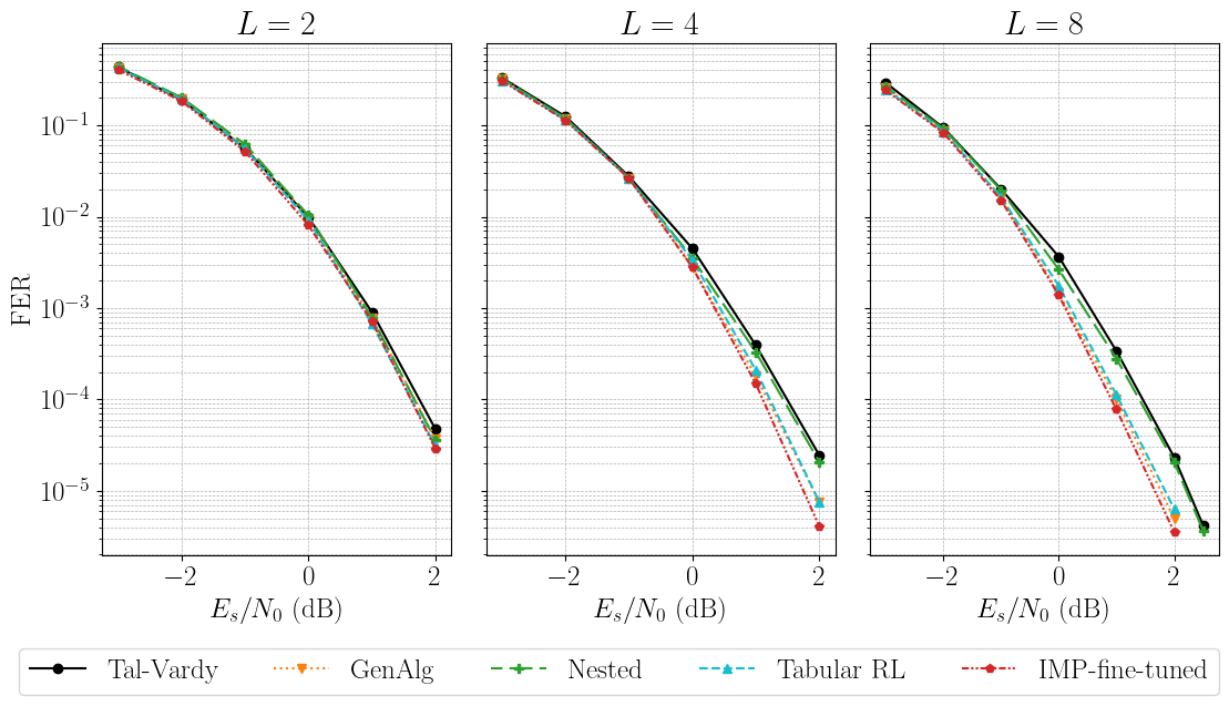
Figure 4: FERs of $\mathcal{P}(64,32,4)$ given by different polar-code construction methods under CA-SCL decoding with list sizes $L=2$ (left); $4$ (middle); $8$ (right). The CRC polynomial is 0x3.

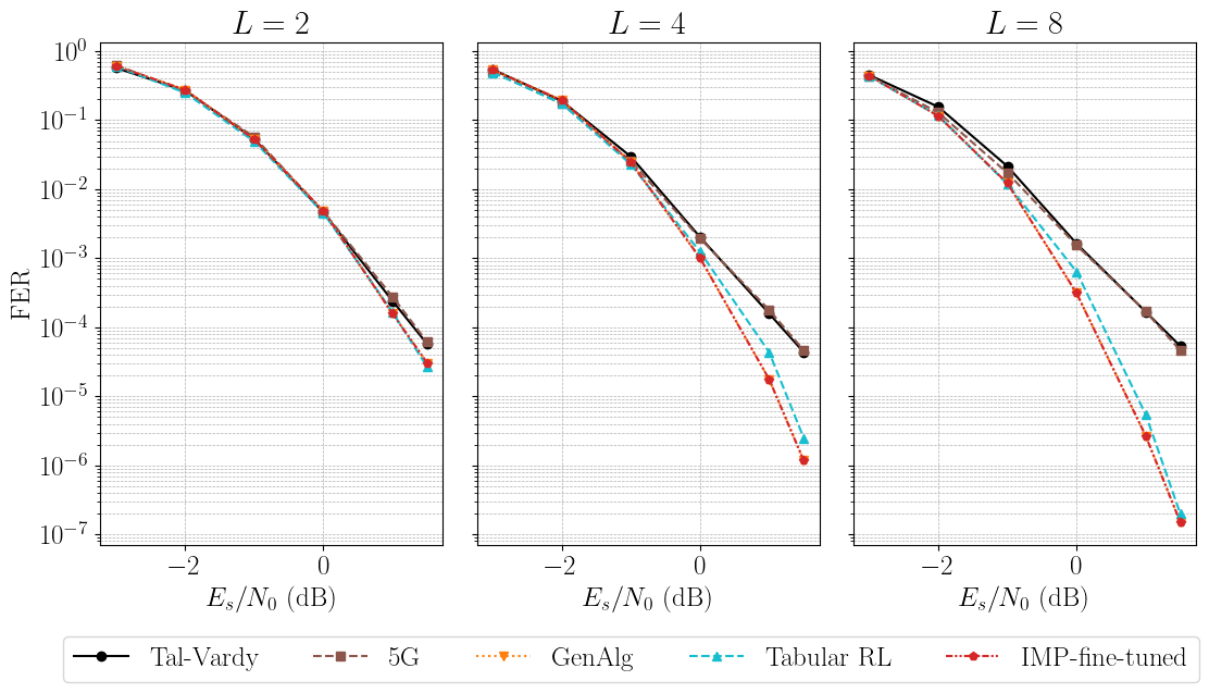
Figure 5: FERs of $\mathcal{P}(128,64,4)$ given by different polar-code construction methods under CA-SCL decoding with list sizes $L=2$ (left); $4$ (middle); $8$ (right). The CRC polynomial is 0x3.

Figs. 4 and 5 compare the FER of the learned constructions by the IMP algorithm with pointwise fine-tuning to the constructions given by the Tal-Vardy’s method [11], the 5G NR standard [18], the GenAlg [35], the nested polar-code construction method [37], and the tabular RL method [38] for $\mathcal{P}(64,32,4)$ and $\mathcal{P}(128,64,4)$, respectively. At each $\gamma_{\mathrm{eval}}$, a polar code tailored for design SNR $\gamma_{\mathrm{eval}}$ is generated by each of the construction methods, and then evaluated by CA-SCL decoding at the same SNR $\gamma_{\mathrm{eval}}$. Since the constructions are channel-dependent, the polar codes corresponding to different $\gamma_{\mathrm{eval}}$ are potentially different, even when they are generated by the same construction method. The training SNR before fine-tuning is selected uniformly at random from the range $[-3,0.5]$ dB in each episode for $\mathcal{P}(64,32,4)$, and the corresponding training SNR range is $[-2.5,0.5]$ dB for $\mathcal{P}(128,64,4)$.

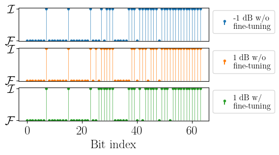
Figure 6: $\mathcal{P}(64,32,4)$ constructed by the “IMP-$[-3.0,0.5]$-L$4$” model evaluated at $\gamma_{\mathrm{eval}}=-1$ dB (top) and $\gamma_{\mathrm{eval}}=1$ dB (middle), and $\mathcal{P}(64,32,4)$ constructed by the “IMP-fine-tuned” model at $\gamma_{\mathrm{eval}}=1$ dB (bottom).

Figs. 4 and 5 show that the constructions from the IMP-fine-tuned method outperform Tal-Vardy’s and 5G constructions in all evaluated scenarios under CA-SCL decoding with various list sizes $L$. The improvement in FER increases with $L$. Figs. 4 and 5 also show that the polar codes constructed by the IMP-fine-tuned model achieve the lowest FER among codes generated by these considered benchmark methods tailored for CA-SCL decoding. For a given $\gamma_{\mathrm{eval}}$ and a given decoding list size $L$, the IMP algorithm with fine-tuning finds the same $\mathcal{P}(128,64,4)$ as the GenAlg does. When the two algorithms identify the same polar codes at a given $\gamma_{\mathrm{eval}}$, the IMP algorithm still shows its advantage over the GenAlg in the sense that the $\gamma_{\mathrm{eval}}$ values that are not seen during training can be directly fed into the same trained IMP model to generate corresponding polar codes. In contrast, re-training is needed for the GenAlg model when $\gamma_{\mathrm{eval}}$ deviates from the design SNR.

V-B Generalization in Design SNRs and List Sizes

This section illustrates the IMP model’s generalization to various design SNRs and to different list sizes without fine-tuning. Since the target SNR is one of IMP model’s input features, a single trained IMP model can automatically provide different constructions at different target SNRs. For example, Fig. 6 shows that the two polar codes generated by the same “IMP-$[-3.0,0.5]$-L$4$” model evaluated at $\gamma_{\mathrm{eval}}=-1$ dB and $\gamma_{\mathrm{eval}}=1$ dB are distinct.

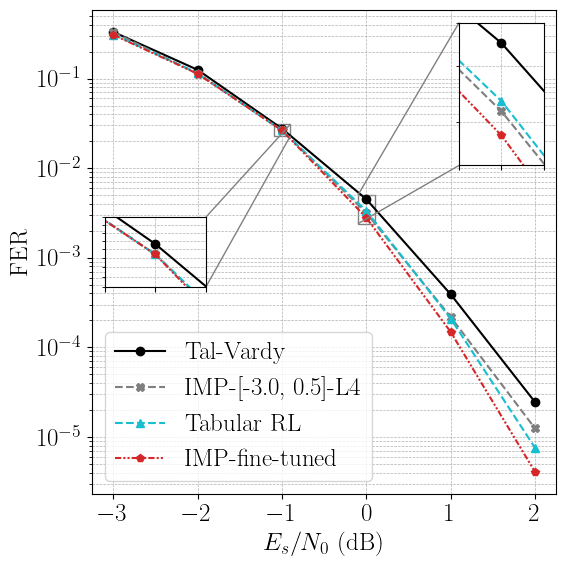
(a) FER of $\mathcal{P}(64,32,4)$ under CA-SCL decoding with $L=4$. The degree-4 CRC polynomial is 0x3.

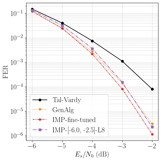
(b) FER of $\mathcal{P}(128,32,4)$ under CA-SCL decoding with $L=8$. The degree-4 CRC polynomial is 0x3.

Figure 7: Comparison of polar codes constructed by the IMP model with and without fine-tuning.

Fig. 7(a) shows constructions of $\mathcal{P}(64,32,4)$ for CA-SCL decoding with $L=4$, in which the “IMP-fine-tuned” models use the “IMP-$[-3.0,0.5]$-L$4$” model as the starting point of fine tuning. Fig. 7(a) shows that the IMP model trained over the SNR range $[-3,0.5]$ dB without fine-tuning can generate constructions that outperform the Tal-Vardy’s constructions over a large range of design SNRs, even when $\gamma_{\mathrm{eval}}$ is outside the training SNR range of $[-3,0.5]$ dB. Also, at some evaluation points, e.g., $\gamma_{\mathrm{eval}}=-1$ dB, the IMP model without fine-tuning already finds the same construction as the tabular RL and as the fine-tuned model, while the latter two are trained specifically for that single $\gamma_{\mathrm{eval}}$ point. These observations indicate that the IMP model learns the general rules for constructing polar codes tailored for a given CA-SCL decoder, and that these learned rules can be applied to a wide range of design SNRs, even to SNRs outside the training SNR range. On the other hand, Fig. 7(a) shows that the additional fine-tuning at each evaluation point can effectively improve the learned construction in most cases, especially when the evaluation point is outside the IMP model’s initial training range as evident in the bottom two cases in Fig. 6.

Similar observations follow from Fig. 7(b) for $\mathcal{P}(128,32,4)$ under CA-SCL decoding with $L=8$. Specifically, the IMP model without fine-tuning outperforms Tal-Vardy’s method, and fine-tuning can further improve the constructed codes. However, in Fig. 7(b), a strictly positive gap is observed between the performance of the trained IMP model over the entire SNR range and the pointwise fine-tuned models, indicating that the trained IMP model is strictly sub-optimal without fine-tuning even within the training SNR range. This gap is mainly caused by the wide training SNR range of $[-6,-2.5]$ dB, in which the FER spans about five orders of magnitude. Due to the wide FER span, the current IMP model fails to generate accurate priority metrics for all training scenarios. This suggests that a more expressive NN architecture might improve the IMP model when fitting a single IMP model to a wide SNR (and consequently FER) range (e.g., several orders of FER magnitude).

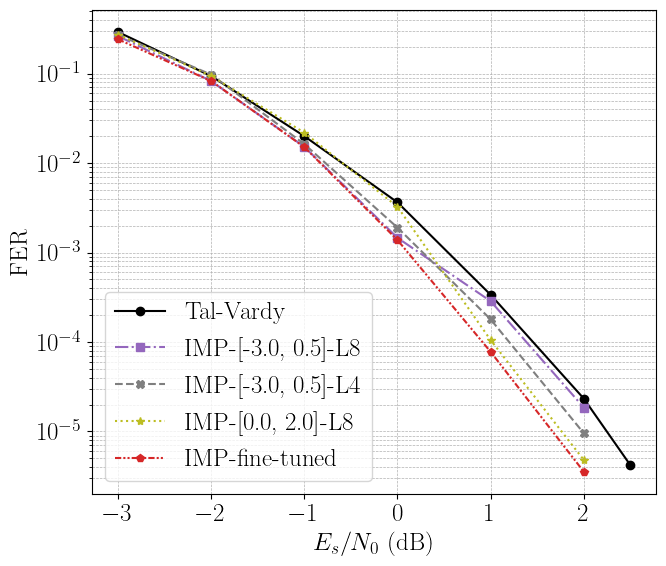
Figure 8: FER performance of $\mathcal{P}(64,32,4)$ given by different polar-code construction methods under CA-SCL decoding with $L=8$. The degree-4 CRC polynomial is 0x3.

Fig. 8 compares different construction methods for $\mathcal{P}(64,32,4)$ under CA-SCL decoding with $L=8$. The “IMP-$[-3.0,0.5]$-L$8$” model is fine tuned to obtain the “IMP-fine-tuned” models. Both “IMP-$[-3.0,0.5]$-L$8$” and “IMP-$[0.0,2.0]$-L$8$” models provide constructions that outperform Tal-Vardy’s constructions over the entire evaluation SNR range, though the improvement is minimal for both models when $\gamma_{\mathrm{eval}}$ is outside the training ranges. Again, fine-tuning helps to find good codes with even lower FERs. Fig. 8’s FER curves for the model “IMP-$[-3.0,0.5]$-L$8$” and the model “IMP-$[0.0,2.0]$-L$8$” intersect between $0$ dB and $1$ dB SNR. This implies that if the IMP model is applied without fine-tuning, better constructions are expected when the design SNR is within the training SNR range.

Fig. 8 also shows the effect of decoding scheme mismatch during training and evaluation. Specifically, under the CA-SCL decoding with $L=8$, the FER of polar codes constructed by the “IMP-$[-3.0,0.5]$-L$4$” model is contrasted with that of polar codes constructed by the “IMP-$[-3.0,0.5]$-L$8$” model. With the same training SNR range, the polar codes constructed by the latter IMP model have lower FER compared to the polar codes constructed by the former one when evaluated within the training SNR range. This suggests that the constructions given by the trained IMP model is effectively tailored for the decoding scheme during training. On the other hand, the codes constructed by the “IMP-$[-3.0,0.5]$-L$4$” model show constantly lower FERs than the Tal-Vardy’s constructions under the CA-SCL decoding with $L=8$, meaning that the IMP models trained for one CA-SCL decoding scheme likely provide constructions that are also reasonably good in FER performance under CA-SCL decoding with different list sizes.

V-C Scalability in $N$ and $K$

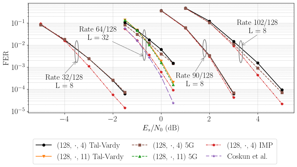
Figure 9: Generalization of “IMP-$[-3.0,0.5]$-L$4$-N$128$-K$64$” model to $N=128$ and different values of $K$. The Tal-Vardy, 5G, and IMP constructions are evaluated by CA-SCL decoding. SCL decoding is used to evaluate the performance of dRM [48] and the polar codes given by Coşkun et al. in [21]. A 4-bit CRC with polynomial 0x3 is used in all four cases for the IMP constructions, and in the $L=8$ cases for the Tal-Vardy and 5G constructions. For the rate-$1/2$, $L=32$ case, 5G CRC-11 is adopted to evaluate Tal-Vardy and 5G constructions.

Fig. 9 applies directly the “IMP-$[-3.0,0.5]$-L$4$” model trained on $\mathcal{P}(128,64,4)$ to construct polar codes with $N=128$ and various values of $K$ without additional training. The IMP model is relabeled as “IMP-$[-3.0,0.5]$-L$4$-N$128$-K$64$” for better clarity.

For the rate-$1/2$ case, the constructions of $\mathcal{P}(128,68,4)$ given by the “IMP-$[-3.0,0.5]$-L$4$-N$128$-K$64$” model is compared against $\mathcal{P}(128,68,4)$ and $\mathcal{P}(128,75,11)$ given by the 5G ordering and Tal-Vardy’s method under CA-SCL decoding with $L=32$. In particular, for Tal-Vardy’s method and the IMP algorithm, the polar codes are constructed separately at each $\gamma_{\mathrm{eval}}$. The performance of the polar code with $N=128$ and $K=64$ given by Coşkun et al. in [21] under SCL with $L=32$ is also included for comparison, in which dynamic frozen bits are utilized. As Fig. 9 depicts, the IMP-based constructions clearly outperform the constructions given by 5G and Tal-Vardy, even when a longer CRC is used to aid the decoding for the latter two methods. In comparison to the polar-code designs with dynamic frozen bits, the IMP-based constructions decoded by CA-SCL with $4$-bit CRC show similar performance in the low SNR regime, while the dynamic-frozen-bit-enabled polar codes achieve lower FER than the IMP-based codes in the high SNR regime.

Besides the rate-$1/2$ case, the constructions of $\mathcal{P}(128,36,4)$, $\mathcal{P}(128,94,4)$ and $\mathcal{P}(128,106,4)$ given by 5G, Tal-Vardy, and the “IMP-$[-3.0,0.5]$-L$4$-N$128$-K$64$” model are compared under CA-SCL decoding with $L=8$. The IMP-based constructions outperform the corresponding polar codes specified by 5G and Tal-Vardy’s algorithm for all these three $K$ values.

Note that no additional training is included in the IMP construction of polar codes with different values of $K\neq 64$. The observation that such IMP-based constructions outperform the 5G and Tal-Vardy’s construction schemes, and that these constructions achieve comparable performance to the polar code designs with dynamic frozen bits indicate IMP’s good generalization capability to different $K$ values. In other words, a single trained IMP model directly finds polar codes with various code rates that achieve reasonably good performance under CA-SCL decoding.

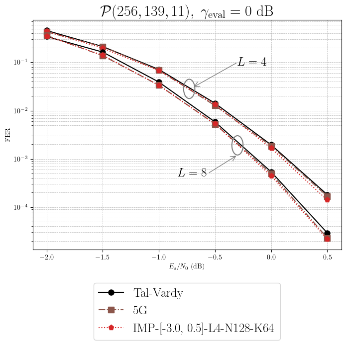
(a) $\mathcal{P}(256,139,11)$ codes with design SNR at $0$ dB.

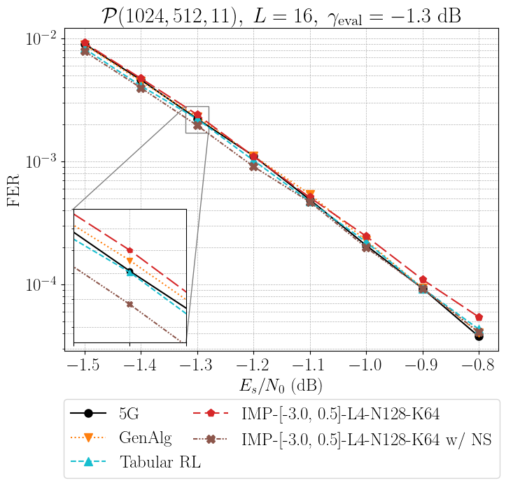
(b) $\mathcal{P}(1024,512,11)$ codes with design SNR at $-1.3$ dB.

Figure 10: FER performance of applying a trained IMP model to different $N$’s without fine-tuning. The 5G CRC-11 with polynomial 0x621 is adopted in evaluation.

Fig. 10 illustrates IMP’s scalability by using the trained “IMP-$[-3.0,0.5]$-L$4$-N$128$-K$64$” model to construct polar codes with larger blocklengths $N=256$ and $1024$. The design SNR for all methods is fixed at $\gamma_{\mathrm{eval}}=0$ dB for $N=256$ case, and $\gamma_{\mathrm{eval}}=-1.3$ dB for $N=1024$ case, respectively, and the constructed codes are evaluated over the entire SNR range. The polar-code construction for the curve labeled “IMP-$[-3.0,0.5]$-L$4$-N$128$-K$64$” is obtained by feeding the corresponding $N$, $K$, $\gamma_{\mathrm{eval}}$ values to the IMP model, which is trained only on $N=128$, $K=64$. For the $N=256$ case in Fig. 10(a), applying the trained IMP model immediately provides polar codes with slightly better performance compared to Tal-Vardy’s and 5G polar code under CA-SCL decoding with $L=4$ and $L=8$, both at $\gamma_{\mathrm{eval}}$ and at various other evaluated SNR values. For the $N=1024$ case as shown in Fig. 10(b), the direct generalization of the trained IMP model shows similar performance comparing to the 5G construction. The SNR gap at FER $2\times 10^{-3}$ between the IMP construction and both the 5G polar code and the tabular RL construction is $0.01$ dB; the corresponding gap between the IMP and GenAlg constructions is less than $0.005$ dB, while both tabular RL and GenAlg methods are trained on $N=1024$, $K=512$, $\gamma=-1.3$ dB directly.

Further improvement in the $N=1024$ case occurs by adding an additional neighborhood search (NS) over the input SNRs, i.e., the values of $x_{u}$ for all variable nodes $u\in\mathcal{Y}_{N}$, to the IMP model. In particular, five SNR values $\{-1.5,-1.4,-1.3,-1.2,-1.1\}$ are fed into the trained IMP model to generate five candidate constructions. These candidates are then evaluated with CA-SCL decoding and $\text{SNR}=-1.3$ dB, and the construction that achieves the lowest FER is selected as the final outcome. Note that the NS process evaluates a fixed trained IMP model for several times, and does not change the trainable parameters of the model. In other words, no training is included in NS. The complexity of NS for $t_{\mathrm{ns}}$ neighboring SNR values is $\mathcal{O}(t_{\mathrm{ns}}M(N-K)(N^{2}d_{\max}+Nd_{\max}^{2})+t_{\mathrm{ns}}\epsilon^{-1}LN\log N)$, where $\epsilon$ is the achievable FER at the design SNR.

Fig. 10(b) shows that NS helps find constructions with lower FER at $-1.3$ dB SNR. More specifically, the polar-code construction found with NS outperforms 5G polar code, the tabular RL construction, and the GenAlg construction at the design SNR $-1.3$ dB. The adopted IMP model, in particular, applies with no additional training on $N$, $K$, and $\gamma_{\mathrm{eval}}$. These observations verify the IMP model’s scalability to different blocklengths without additional training.

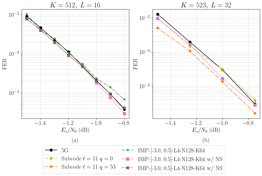
Figure 11: (a) Effect of NS on $\mathcal{P}(1024,512,11)$ under CA-SCL decoding with $L=16$. (b) Performance of IMP with NS on $\mathcal{P}(1024,523,11)$ under CA-SCL decoding with $L=32$.

Fig. 11 further shows NS’s effect on the IMP model for blocklength $N=1024$ that is unseen during training of the “IMP-$[-3.0,0.5]$-L$4$-N$128$-K$64$” model. $\mathcal{P}(1024,512,11)$ and $\mathcal{P}(1024,523,11)$ are evaluated. The curve labeled “IMP-$[-3.0,0.5]$-L$4$-N$128$-K$64$” shows the IMP polar codes’ performance when the model’s input SNR matches the evaluation SNR, while the curve labeled “IMP-$[-3.0,0.5]$-L$4$-N$128$-K$64$ w/ NS” reports the performance of the polar-code constructions after NS at each evaluation SNR.

In Fig. 11a, the direct generalization of a trained IMP model without NS can generate polar codes that achieve the same order of FER magnitude as the 5G polar codes. This indicates that the IMP model learns some general polar-code-construction rules that apply to various blocklengths. Nevertheless, the FER of IMP polar codes without NS may be higher than that of the 5G polar code, and there is no guarantee or prior knowledge of whether the IMP model without NS provides a satisfying polar-code construction for a target $(N,K,\gamma)$ when the target blocklength $N$ is never seen by the IMP model during training. The lack of performance guarantee in generalization is a major limitation of the current IMP algorithm. NS is used as a simple remedy for this limitation that requires no additional training. As Fig. 11a shows, in many cases, a polar-code construction with a lower FER can be found by evaluating several neighboring SNR points, and the reported polar codes after NS can outperform the 5G polar code.

In Fig. 11b, the constructions given by IMP with NS for the $K=523$ case are compared against the randomized polar subcode [25], which exploits constructions with dynamic frozen bits and uses the sequential decoder. The parameter $t$ in [25] represents the number of dynamic frozen bits that are dependent on previous information bits, and $q$ represents the number of dynamic (random) freezing constraints, so the design exploits $t+q$ dynamic frozen bits in total. To achieve a fair comparison, this work selects $t=11$ to match the CRC length, and the sequential decoder’s list size $L=32$ to match the CA-SCL decoder’s list size. The figure again shows that IMP with NS finds constructions that achieve lower FER than 5G polar code, and these IMP-with-NS constructions show better performance comparing to the randomized polar subcode when $t$ matches the CRC length and $q=0$. The randomized polar subcode outperforms IMP with NS when $q=53$. This is expected because the randomized polar subcode allows more flexibility in the frozen-bit values and needs a more sophisticated list decoder.

VI Conclusion

This paper proposes a GNN-based polar-code construction algorithm, named the IMP algorithm. A salient feature of the IMP algorithm is that a single trained IMP model directly applies to constructions for various design SNRs and different blocklengths without any additional training. This feature makes the IMP algorithm a powerful candidate in real-world deployment, in which the wireless channel condition varies over time and searching for good polar codes for each design requirement separately can be complicated and costly.

There exist some limitations in the current IMP algorithm such as the lack of a general performance guarantee to scenarios that are not seen by the model during training and the high evaluation complexity, and these merit further investigation. Nonetheless, the IMP algorithm illustrates the potential of using GNN as a tool for code design problems. Some future research directions using similar methods may include: (a) polar-code constructions on different channels such as fading channels; (b) variations of the graph structures and initial local messages, e.g., different connection patterns among check nodes, and using Bhattacharyya parameters as the check nodes’ initial messages, etc; (c) graph-based algorithms that enable joint learning over non-frozen set and CRC design; and (d) GNN-based code designs tailored for other decoding algorithms such as BP decoding, or for other outer codes.

References

- [1] E. Arıkan, “Channel polarization: A method for constructing capacity-achieving codes for symmetric binary-input memoryless channels,” IEEE Trans. Inf. Theory, vol. 55, no. 7, pp. 3051–3073, Jul. 2009.
- [2] I. Tal and A. Vardy, “List decoding of polar codes,” IEEE Trans. Inf. Theory, vol. 61, no. 5, pp. 2213–2226, May 2015.
- [3] M. C. Coşkun, G. Durisi, T. Jerkovits, G. Liva, W. Ryan, B. Stein, and F. Steiner, “Efficient error-correcting codes in the short blocklength regime,” Physical Commun., vol. 34, pp. 66 – 79, Jun. 2019.
- [4] E. Arıkan, “From sequential decoding to channel polarization and back again,” Sep. 2019. [Online]. Available: http://arxiv.org/abs/1908.09594
- [5] H. Yao, A. Fazeli, and A. Vardy, “List decoding of Arıkan’s pac codes,” Entropy, vol. 23, no. 7, Jun. 2021.
- [6] 3GPP, “Final report of 3GPP TSG RAN WG1 #87 v1.0.0,” Reno, USA, Nov. 2016.
- [7] H. Li and J. Yuan, “A practical construction method for polar codes in AWGN channels,” in IEEE 2013 Tencon - Spring, 2013, pp. 223–226.
- [8] R. Mori and T. Tanaka, “Performance and construction of polar codes on symmetric binary-input memoryless channels,” in Proc. IEEE Int. Symp. Inf. Theory (ISIT), Jun. 2009, pp. 1496–1500.
- [9] ——, “Performance of polar codes with the construction using density evolution,” IEEE Commun. Lett., vol. 13, no. 7, pp. 519–521, Jul. 2009.
- [10] P. Trifonov, “Efficient design and decoding of polar codes,” IEEE Trans. Commun., vol. 60, no. 11, pp. 3221–3227, Nov. 2012.
- [11] I. Tal and A. Vardy, “How to construct polar codes,” IEEE Trans. Inf. Theory, vol. 59, no. 10, pp. 6562–6582, Oct. 2013.
- [12] S. Sun and Z. Zhang, “Designing practical polar codes using simulation-based bit selection,” IEEE J. Emerging and Sel. Topics in Circuits and Syst., vol. 7, no. 4, pp. 594–603, Dec. 2017.
- [13] M. Bardet, V. Dragoi, A. Otmani, and J.-P. Tillich, “Algebraic properties of polar codes from a new polynomial formalism,” in Proc. IEEE Int. Symp. Inf. Theory (ISIT), Jul. 2016, pp. 230–234.
- [14] C. Schürch, “A partial order for the synthesized channels of a polar code,” in Proc. IEEE Int. Symp. Inf. Theory (ISIT), Jul. 2016, pp. 220–224.
- [15] M. Mondelli, S. H. Hassani, and R. L. Urbanke, “Construction of polar codes with sublinear complexity,” IEEE Trans. Inf. Theory, vol. 65, no. 5, pp. 2782–2791, May 2019.
- [16] G. He, J. Belfiore, I. Land, G. Yang, X. Liu, Y. Chen, R. Li, J. Wang, Y. Ge, R. Zhang, and W. Tong, “Beta-expansion: A theoretical framework for fast and recursive construction of polar codes,” in IEEE Global Commun. Conf. (GLOBECOM), Dec. 2017, pp. 1–6.
- [17] M. Mondelli, S. H. Hassani, and R. L. Urbanke, “From polar to Reed-Muller codes: A technique to improve the finite-length performance,” IEEE Trans. Commun., vol. 62, no. 9, pp. 3084–3091, Sep. 2014.
- [18] 3rd Generation Partnership Project (3GPP), “Multiplexing and channel coding,” 3GPP, TS 38.212, 2018, version 15.3.0.
- [19] N. Hussami, S. B. Korada, and R. Urbanke, “Performance of polar codes for channel and source coding,” in Proc. IEEE Int. Symp. Inf. Theory (ISIT), Jun. 2009, pp. 1488–1492.
- [20] H. Yao, A. Fazeli, and A. Vardy, “A deterministic algorithm for computing the weight distribution of polar codes,” in Proc. IEEE Int. Symp. Inf. Theory (ISIT), Jul. 2021, pp. 1218–1223.
- [21] M. C. Coşkun and H. D. Pfister, “An information-theoretic perspective on successive cancellation list decoding and polar code design,” IEEE Trans. Inf. Theory, vol. 68, no. 9, pp. 5779–5791, Sep. 2022.
- [22] T. Wang, D. Qu, and T. Jiang, “Parity-check-concatenated polar codes,” IEEE Commun. Lett., vol. 20, no. 12, pp. 2342–2345, Dec. 2016.
- [23] H. Zhang, R. Li, J. Wang, S. Dai, G. Zhang, Y. Chen, H. Luo, and J. Wang, “Parity-check polar coding for 5G and beyond,” in 2018 IEEE Int. Conf. Commun. (ICC), May 2018, pp. 1–7.
- [24] P. Trifonov and V. Miloslavskaya, “Polar subcodes,” IEEE J. Select. Areas Commun., vol. 34, no. 2, pp. 254–266, Feb. 2015.
- [25] P. Trifonov and G. Trofimiuk, “A randomized construction of polar subcodes,” in Proc. IEEE Int. Symp. Inf. Theory (ISIT), Aug. 2017, pp. 1863–1867.
- [26] P. Trifonov, “Randomized polar subcodes with optimized error coefficient,” IEEE Trans. Commun., vol. 68, no. 11, pp. 6714–6722, Nov. 2020.
- [27] M.-C. Chiu, “Interleaved polar (i-polar) codes,” IEEE Trans. Inf. Theory, vol. 66, no. 4, pp. 2430–2442, Apr. 2020.
- [28] M. Rowshan, S. H. Dau, and E. Viterbo, “Error coefficient-reduced polar/pac codes,” Nov. 2021. [Online]. Available: http://arxiv.org/abs/2111.08843v2
- [29] V. Miloslavskaya, B. Vucetic, Y. Li, G. Park, and O.-S. Park, “Recursive design of precoded polar codes for SCL decoding,” IEEE Trans. Commun., vol. 69, no. 12, pp. 7945–7959, Dec. 2021.
- [30] B. Li, J. Gu, and H. Zhang, “Performance of CRC concatenated pre-transformed RM-polar codes,” Apr. 2021. [Online]. Available: http://arxiv.org/abs/2104.07486v1
- [31] M. Qin, J. Guo, A. Bhatia, A. Guillén i Fàbregas, and P. H. Siegel, “Polar code constructions based on LLR evolution,” IEEE Commun. Lett., vol. 21, no. 6, pp. 1221–1224, Jun. 2017.
- [32] B. Li, H. Shen, and D. Tse, “A RM-polar codes,” arXiv, Jul. 2014.
- [33] P. Yuan, T. Prinz, G. Böcherer, O. Iscan, R. Boehnke, and W. Xu, “Polar code construction for list decoding,” in VDE 12th Int. ITG Conf. Syst., Commun. and Coding, Feb. 2019, pp. 1–6.
- [34] M. Ebada, S. Cammerer, A. Elkelesh, and S. ten Brink, “Deep learning-based polar code design,” in IEEE 57th Annual Allerton Conf. Commun., Control, and Computing (Allerton), Sep. 2019, pp. 177–183.
- [35] A. Elkelesh, M. Ebada, S. Cammerer, and S. t. Brink, “Decoder-tailored polar code design using the genetic algorithm,” IEEE Trans. Commun., vol. 67, no. 7, pp. 4521–4534, Jul. 2019.
- [36] L. Huang, H. Zhang, R. Li, Y. Ge, and J. Wang, “AI coding: Learning to construct error correction codes,” IEEE Trans. Commun., vol. 68, no. 1, pp. 26–39, Jan. 2020.
- [37] Y. Li, Z. Chen, G. Liu, Y.-C. Wu, and K.-K. Wong, “Learning to construct nested polar codes: An attention-based set-to-element model,” IEEE Commun. Lett., vol. 25, no. 12, pp. 3898–3902, Dec. 2021.
- [38] Y. Liao, S. A. Hashemi, J. M. Cioffi, and A. Goldsmith, “Construction of polar codes with reinforcement learning,” IEEE Trans. Commun., vol. 70, no. 1, pp. 185–198, Jan. 2022.
- [39] L. Huang, H. Zhang, R. Li, Y. Ge, and J. Wang, “Reinforcement learning for nested polar code construction,” in 2019 IEEE Global Commun. Conf. (GLOBECOM), Dec. 2019, pp. 1–6.
- [40] F. Scarselli, M. Gori, A. C. Tsoi, M. Hagenbuchner, and G. Monfardini, “The graph neural network model,” IEEE Trans. Neural Networks, vol. 20, no. 1, pp. 61–80, Jan. 2009.
- [41] J. Zhou, G. Cui, S. Hu, Z. Zhang, C. Yang, Z. Liu, L. Wang, C. Li, and M. Sun, “Graph neural networks: A review of methods and applications,” AI Open, vol. 1, pp. 57–81, 2020.
- [42] Z. Wu, S. Pan, F. Chen, G. Long, C. Zhang, and P. S. Yu, “A comprehensive survey on graph neural networks,” IEEE Trans. Neural Networks and Learning Systems, vol. 32, no. 1, pp. 4–24, Jan. 2021.
- [43] C. Zhang, D. Song, C. Huang, A. Swami, and N. V. Chawla, “Heterogeneous graph neural network,” in Proc. the 25th ACM SIGKDD Int. Conf. Knowledge Discovery & Data Mining, Aug. 2019, pp. 793–803.
- [44] V. Mnih, K. Kavukcuoglu, D. Silver, A. Graves, I. Antonoglou, D. Wierstra, and M. Riedmiller, “Playing atari with deep reinforcement learning,” arXiv preprint arXiv:1312.5602, Dec. 2013.
- [45] W. L. Hamilton, “Graph representation learning,” Synthesis Lectures on Artificial Intelligence and Machine Learning, vol. 14, no. 3, pp. 1–159, Sep. 2020.
- [46] J. Gilmer, S. S. Schoenholz, P. F. Riley, O. Vinyals, and G. E. Dahl, “Neural message passing for quantum chemistry,” in Int. Conf. Machine Learning. PMLR, July 2017, pp. 1263–1272.
- [47] W. Hamilton, Z. Ying, and J. Leskovec, “Inductive representation learning on large graphs,” Adv. Neural Inf. Process. Syst., vol. 30, 2017.
- [48] M. C. Coşkun, J. Neu, and H. D. Pfister, “Successive cancellation inactivation decoding for modified Reed-Muller and eBCH codes,” in Proc. IEEE Int. Symp. Inf. Theory (ISIT). IEEE, Jun. 2020, pp. 437–442.