Generalized Henneberg stable minimal surfaces

Abstract

We generalize the classical Henneberg minimal surface by giving an infinite family of complete, finitely branched, non-orientable, stable minimal surfaces in $\mathbb{R}^{3}$. These surfaces can be grouped into subfamilies depending on a positive integer (called the complexity), which essentially measures the number of branch points. The classical Henneberg surface $H_{1}$ is characterized as the unique example in the subfamily of the simplest complexity $m=1$, while for $m\geq 2$ multiparameter families are given. The isometry group of the most symmetric example $H_{m}$ with a given complexity $m\in\mathbb{N}$ is either isomorphic to the dihedral isometry group $D_{2m+2}$ (if $m$ is odd) or to $D_{m+1}\times\mathbb{Z}_{2}$ (if $m$ is even). Furthermore, for $m$ even $H_{m}$ is the unique solution to the Björling problem for a hypocycloid of $m+1$ cusps (if $m$ is even), while for $m$ odd the conjugate minimal surface $H_{m}^{*}$ to $H_{m}$ is the unique solution to the Björling problem for a hypocycloid of $2m+2$ cusps.

1 Introduction

A celebrated result obtained independently by do Carmo & Peng [1], Fischer-Colbrie & Schoen [2] and Pogorelov [7] establishes that if $M$ is a complete orientable stable minimal surface in $\mathbb{R}^{3}$, then $M$ is a plane. Ros [8] proved that the same characterization holds without assuming orientability. Nevertheless, a plethora of complete stable minimal surfaces in $\mathbb{R}^{3}$ appear if we allow these stable minimal surfaces to have branch points, with the simplest example being the classical Henneberg minimal surface [3].

The class of complete, finitely connected and finitely branched minimal surfaces with finite total curvature (among which stable ones are a particular case) appears naturally in the following situation: Given ${\varepsilon}_{0}>0$, $I\in\mathbb{N}\cup\{0\}$ and $H_{0},K_{0}\geq 0$, let $\Lambda=\Lambda(I,H_{0},{\varepsilon}_{0},K_{0})$ be the set of immersions $F\colon M\looparrowright X$ where $X$ is a complete Riemannian 3-manifold with injectivity radius $\mbox{\rm Inj}(X)\geq{\varepsilon}_{0}$ and absolute sectional curvature bounded from above by $K_{0}$, $M$ is a complete surface, $F$ has constant mean curvature $H\in[0,H_{0}]$ and Morse index at most $I$. The second fundamental form $|A_{F_{n}}|$ of a sequence $\{F_{n}\}_{n}\subset\Lambda$ may fail to be uniformly bounded, which leads to lack of compactness of $\Lambda$. Nevertheless, the interesting ambient geometry of the immersions $F_{n}$ can be proven to be well organized locally around at most $I$ points $p_{1,n},\ldots,p_{k,n}\in M_{n}$ ($k\leq I$) where $|A_{F_{n}}|$ takes on arbitrarily large local maximum values. Around any of these points $p_{i,n}$, one can perform a blow-up analysis and find a limit of (a subsequence of) expansions ${\lambda}_{n}F_{n}$ of the $F_{n}$ (that is, we view $F_{n}$ as an immersion with constant mean curvature $H_{n}/{\lambda}_{n}$ in the scaled ambient manifold ${\lambda}_{n}X_{n}$ for a sequence $\{{\lambda}_{n}\}_{n}\subset\mathbb{R}^{+}$ tending to $\infty$). This limit is a complete immersed minimal surface $f\colon\Sigma\looparrowright\mathbb{R}^{3}$ with finite total curvature, passing through the origin $\vec{0}\in\mathbb{R}^{3}$. Recall that such an $f$ has finitely many ends, each of which is a multi-valued graph of finite multiplicity (spinning) $s\in\mathbb{N}$, over the exterior of a disk in the tangent plane at infinite for $f$ at that end. Thus, arbitrarily small almost perfectly formed copies of large compact portions of $f(\Sigma)$ can be reproduced in $F_{n}(M_{n})$ around $F_{n}(p_{i,n})$ for $n$ sufficiently large. Complete, finitely connected and finitely branched minimal surfaces with finite total curvature in $\mathbb{R}^{3}$ appear naturally when considering clustering phenomena in this framework: It may occur that different blow-up limits of the $F_{n}$ around $p_{i,n}$ at different scales ${\lambda}_{1,n}>{\lambda}_{2,n}$ with ${\lambda}_{1,n}/{\lambda}_{2,n}\to\infty$ as $n\to\infty$, produce different limits $f_{j}\colon\Sigma_{j}\looparrowright\mathbb{R}^{3}$, $j=1,2$, with Index$(f_{1})+\mbox{Index}(f_{2})\leq I$; in this case, all the geometry of $f_{1}(\Sigma_{1})$ collapses around $\vec{0}\in f_{2}(\Sigma_{2})$, and every end of $f_{1}(\Sigma_{1})$ with multiplicity $m\geq 3$ produces a branch point at the origin for $f_{2}(\Sigma_{2})$ of branching order $s-1$. For details about this clustering phenomenon and how to organize these blow-up limits in hierarchies appearing around $\{p_{i,n}\}_{n}$, see the paper [4] by Meeks and the second author.

The main goal of this paper is to generalize the classical Henneberg minimal surface $H_{1}$ to an infinite family of connected, 1-sided, complete, finitely branched, stable minimal surfaces in $\mathbb{R}^{3}$. Branch points are unavoidable if we seek for complete, non-flat stable minimal surfaces by the aforementioned results [1, 2, 7, 8]; 1-sidedness is also necessary condition for stability (see Proposition 3 below). Our examples can be grouped into subfamilies depending on the number of branch points (this will be encoded by an integer $m\in\mathbb{N}$ called the complexity). The most symmetric examples $H_{m}$ in each subfamily of complexity $m$ will be studied in depth (Section 5.3). Depending on the parity of $m$, either $H_{m}$ or its conjugate minimal surface $H_{m}^{*}$ (which does not gives rise to a 1-sided surface, see Section 5.4) can be viewed as the unique solution of a Björling problem for a planar hypocycloid (Section 5.7). The isometry group of $H_{m}$ is isomorphic to the dihedral group $D_{2m+2}$ if $m$ is odd and to the group $D_{m+1}\times\mathbb{Z}_{2}$ if $m$ is even (Section 5.8). We will also prove that $H_{1}$ is the only element in the subfamily with complexity $m=1$ (Theorem 11), while for $m\geq 2$, $H_{m}$ can be deformed in multiparameter families: Proposition 14 gives an explicit 1-parameter family of examples with complexity $m=2$, interpolating between $H_{2}$ and a limit which turns out to be $H_{1}$ (Section 6.2.1), and the subfamily of examples with complexity $m=2$ is a two-dimensional real analytic manifold around $H_{2}$ (Section 6.2.2).

2 $1$-sided branched stable minimal surfaces

We start with the Weierstrass data $(g,\omega)$ on a Riemann surface $\Sigma$, so that $(g,\omega)$ solves the period problem and produces a conformal harmonic map $X\colon\Sigma\looparrowright\mathbb{R}^{3}$ given by the classical formula

$$X=\text{Re}\int(\phi_{1},\phi_{2},\phi_{3})=\text{Re}\int\left(\frac{1}{2}(1-g^{2})\omega,\frac{i}{2}(1+g^{2})\omega,g\omega\right).$$ (1)

We will assume that $X$ is an immersion outside of a locally finite set of points ${\mathcal{B}}\subset\Sigma$, where $X$ fails to be an immersion (points of ${\mathcal{B}}$ are called branch points of $X$). Such an $X$ will be called a branched minimal immersion. The induced (possible branched) metric is given by

$$ds^{2}=\frac{1}{4}(1+|g|^{2})^{2}|\omega|^{2}.$$ (2)

The local structure of $X$ around a branch point in ${\mathcal{B}}$ is well-known, see e.g. Micallef and White [5, Theorem 1.4] for details. Given $p\in{\mathcal{B}}$, there exists a conformal coordinate $(D,z)$ for $\Sigma$ centered at $p$ (here $D$ is the closed unit disk in the plane), a diffeomorphism $u$ of $D$ and a rotation $\phi$ of $\mathbb{R}^{3}$ such that $\phi\circ X\circ u$ has the form

$$z\mapsto(z^{q},x(z))\in\mathbb{C}\times\mathbb{R}\sim\mathbb{R}^{3}$$

for $z$ near $0$, where $q\in\mathbb{N}$, $q\geq 2$, $x$ is of class $C^{2}$, and $x(z)=o(|z|^{q})$. In this setting, the branching order of $p$ is defined to be $q-1\in\mathbb{N}$.

Let us assume that $X$ produces a $1$-sided branched minimal surface; this means that there exists an anti-holomorphic involution without fixed points $I:\Sigma\rightarrow\Sigma$ such that $I\circ\phi_{j}=\overline{\phi_{j}}$ for $j=1,2,3$. This is equivalent to

$$-1/\overline{g}=g\circ I,\qquad I^{*}\omega=-\overline{g^{2}\omega}.$$ (3)

In particular, $I$ must preserve the set ${\mathcal{B}}$. $\Sigma/\langle I\rangle$ is a non-orientable differentiable surface endowed with a conformal class of metrics, and the harmonic map $X$ induces another harmonic map $\widehat{X}\colon\Sigma/\langle I\rangle\looparrowright\mathbb{R}^{3}$ such that $\widehat{X}\circ\pi=X$, where $\pi\colon\Sigma\to\Sigma/\langle I\rangle$ is the natural projection ($\widehat{X}$ is a branched minimal immersion). Reciprocally, every $1$-sided conformal harmonic map can be constructed in this way.

Remark 1.

In the particular case that the compactification of $\Sigma$ is $\overline{\mathbb{C}}$, we can assume that $I(z)=-1/\overline{z}$ and write $\omega=f\,dz$ globally. In this setting, the above equations give

$$-1/\overline{g(z)}=g(-1/\overline{z}),\quad f\circ I=-\overline{z^{2}g^{2}f}.$$ (4)

Definition 2.

Given a $1$-sided conformal harmonic map $\widehat{X}\colon\Sigma/\langle I\rangle\looparrowright\mathbb{R}^{3}$, we denote by $\Delta$, $|A|^{2}$ the Laplacian and squared norm of the second fundamental form of $\widehat{X}$. The index of $\widehat{X}$ is defined as the number of negative eigenvalues of the elliptic, self-adjoint operator $L=\Delta+|A|^{2}$ (Jacobi operator of $X$) defined over the space of compactly supported smooth functions $\phi\colon\Sigma\to\mathbb{R}$ such that $\phi\circ I=-\phi$. $\widehat{X}$ is said to be stable if its index is zero.

In the case $\widehat{X}$ is finitely branched, the eigenvalues and eigenfunctions of the Jacobi operator of $X$ are well defined via a variational approach, since the codimension of the singularity set ${\mathcal{B}}$ is two (see [9]), and stability also makes sense.

The next result is proven by Meeks and the second author in [4].

Proposition 3.

Let $X\colon\Sigma\looparrowright\mathbb{R}^{3}$ be complete, non-flat, finitely branched minimal immersion with branch locus ${\mathcal{B}}\subset\Sigma$. Then:

1. [4, Proposition 3] If $X$ is stable, then $\Sigma$ is non-orientable and $X({\mathcal{B}})$ contains more than 1 point.

2. [4, Remark 3.6] Suppose that $\Sigma$ is non-orientable, $X$ has finite total curvature and its extended unoriented Gauss map $G\colon\mathbb{P}^{2}=\mathbb{S}^{2}/\{\pm 1\}\to\mathbb{P}^{2}$ is a diffeomorphism. Then, $X$ is stable.

3 The Björling problem

We next recall the basics of the classical Björling problem, to be used later. Let $\gamma\colon I\subset\mathbb{R}\rightarrow\mathbb{R}^{3}$ be an analytic regular curve and $\eta$ an analytic vector field along $\gamma$ such that $\langle\gamma(t),\eta(t)\rangle=0$ and $\|\eta(t)\|=1$ for all $t\in I$. The classical result due to E.G. Björling asserts that the following parametrization generates a minimal surface $S$ which contains $\gamma$ and has $\eta$ as unit normal vector along $\gamma$:

$$X(u,v)=\text{Re}\left(\widetilde{\gamma}(w)-i\int_{w_{0}}^{w}\widetilde{\eta}(w)\times\widetilde{\gamma}^{\prime}(w)\,dw\right),$$

where $\widetilde{\gamma},\widetilde{\eta}$ are analytic extensions of the corresponding $\gamma,\eta$ and $w=u+iv$ is defined in a simply connected domain $\Omega\subset\mathbb{C}$ with $I\subset\Omega$. In particular, the surface $S$ is locally unique around $\gamma$ with this data (it is called the solution to the Björling problem with data ${\gamma},\eta$).

In what follows, we will consider different Björling problems for analytic planar curves ${\gamma}\subset\{z=0\}$ that fail to be regular at finitely many points. The above construction can be applied to each of the regular arcs of these curves after removing the zeros of ${\gamma}^{\prime}$. In all our applications, $\eta$ will be taken as the (unit) normal vector field to ${\gamma}$ as a planar curve.

4 The classical Henneberg surface

The classical Henneberg minimal surface $H_{1}$ is the $1$-sided, complete, stable minimal surface in $\mathbb{R}^{3}$ given by the Weierstrass data:

$$g(z)=z,\quad\omega=z^{-4}(z\pm i)(z\pm 1)dz=z^{-4}(z^{4}-1)dz,\quad z\in\overline{\mathbb{C}}-\{0,\infty\}.$$ (5)

$H_{1}$ has two branch points at $[1]=\{1,-1\},[i]=\{i,-i\}\in\mathbb{P}^{2}=\overline{\mathbb{C}}/\langle A\rangle$, where $A(z)=-1/\overline{z}$ is the antipodal map. By Proposition 3, $H_{1}$ is stable.

$H_{1}$ can be conformally parameterized (up to translations) by equation (1). After translating $X$ so that $X(e^{i\pi/4})=\vec{0}$, the branch points of $H_{1}$ are mapped by $X$ to $(0,0,\pm 1)$ and a parametrization of $H_{1}$ in polar coordinates $z=re^{i\theta}$ is given by

$$X(re^{i\theta})=\left(\begin{array}[]{c}\frac{\cos\theta}{2}(r-\frac{1}{r})-\frac{\cos(3\theta)}{6}(r^{3}-\frac{1}{r^{3}})\\ -\frac{\sin\theta}{2}(r-\frac{1}{r})-\frac{\sin(3\theta)}{6}(r^{3}-\frac{1}{r^{3}})\\ \frac{\cos(2\theta)}{2}(r^{2}+\frac{1}{r^{2}})\end{array}\right).$$ (6)

Since $X(e^{i\theta})=(0,0,\cos(2\theta))$, then $X$ maps the unit circle into the vertical segment $\{(0,0,t)|\,t\in[-1,1]\}$. In this way, $\theta\in[0,2\pi]\mapsto X(e^{i\theta})$ bounces between the two branch points of $H_{1}$ (observe that the complement of this closed segment in the $x_{3}$-axis is not contained in $H_{1}$), see Figure 1.

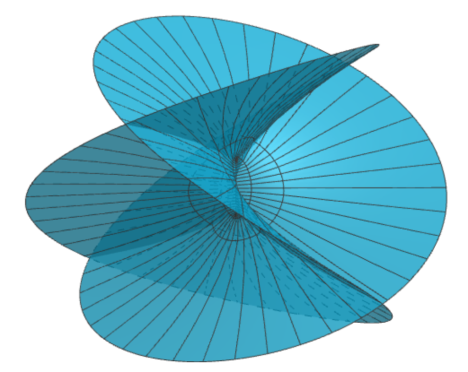
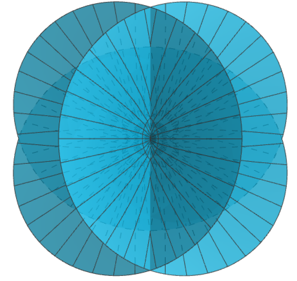
Figure 1: The Henneberg surface $H_{1}$. After a traslation, the branch points of $H_{1}$ are contained in the $x_{3}$-axis. $H_{1}$ contains two horizontal, orthogonal lines that bisect the $x_{1}$- and $x_{2}$-axis. Left: Intersection of $H_{1}$ with a ball of radius 8. Right: top view of $H_{1}$.

4.1 Isometries of $H_{1}$

It is straightforward to check that

1. The antipodal map $A\colon\overline{\mathbb{C}}\to\overline{\mathbb{C}}$ (in polar coordinates $(r,\theta)\mapsto(1/r,\pi+\theta)$) leaves the surface invariant. This is the deck transformation, which is orientation reversing.

2. The map $z\mapsto-z$ (in polar coordinates $(r,\theta)\mapsto(r,\pi+\theta)$) induces the rotation by angle $\pi$ about the axis $x_{3}$ on the surface.

3. The inversion of the $z$-plane with respect to the unit circle, $z\mapsto 1/z$, (in polar coordinates $(r,\theta)\mapsto(1/r,\theta)$) is the composition of $A$ with $z\mapsto-z$, and thus, it also induces a rotation of angle $\pi$ about the $x_{3}$-axis on the surface.

4. The conjugation map $z\mapsto\overline{z}$ (in polar coordinates $(r,\theta)\mapsto(r,-\theta)$) induces the reflection of $X$ about the plane $(x_{1},x_{3})$.

5. The reflection about the imaginary axis (in polar coordinates $(r,\theta)\mapsto(r,\pi-\theta)$) induces the reflection of $X$ about the plane $(x_{2},x_{3})$.

6. $X$ maps the half-line $\{re^{-i\pi/4}\ |\ r\in(0,\infty)\}$ (respectively $\{re^{i\pi/4}\ |\ r\in(0,\infty)\}$) injectively into $l_{1}=\text{Span}(1,1,0)$ (respectively $l_{2}=\text{Span}(1,-1,0)$). Thus, the rotations $R_{1},R_{2}$ of angle $\pi$ about $l_{1},l_{2}$ are isometries of $X$ ($R_{1}$ is induced by $z\mapsto-i\overline{z}$ and $R_{2}$ by $z\mapsto i\overline{z}$).

7. The map $z\mapsto iz$ (in polar coordinates $(r,\theta)\mapsto(r,\theta+\pi/2)$) induces the rotation of angle $\pi/2$ about the $x_{3}$-axis composed by a reflection in the $(x_{1},x_{2})$-plane.

Together with the identity map, the above isometries form a subgroup of the isometry group Iso$(H_{1})$ of $H_{1}$, isomorphic to the dihedral group $D_{4}$.

Lemma 4.

These are all the (intrinsic) isometries of $H_{1}$.

Proof.

This is a direct consequence of the fact that every intrinsic isometry $\phi$ of $H_{1}$ produces a conformal diffeomorphism of $\mathbb{C}\setminus\{0\}$ into itself that preserves the set of branch points of $H_{1}$. In particular, $\phi$ is of one of the aforementioned eight cases. ∎

4.2 Associated family and the conjugate surface $H_{1}^{*}$.

The flux vector of $H_{1}$ around the origin in $\mathbb{C}$ vanishes (in other words, the Weierstrass form $\Phi=(\phi_{1},\phi_{2},\phi_{3})$ associated to $H_{1}$ is exact). This implies that all associated surfaces $\{\widetilde{H}_{1}(\varphi)\ |\ \varphi\in[0,2\pi)\}$ to the orientable cover $\widetilde{H}_{1}=\widetilde{H}_{1}(0)$ of $H_{1}$ are well-defined as surfaces in $\mathbb{R}^{3}$ (the branched minimal immersion $\widetilde{H}_{1}(\varphi)$ has Weierstrass data $g_{\varphi}=g$, $\omega_{\varphi}=e^{i\varphi}\omega$ and it is isometric to $\widetilde{H}_{1}$, in particular it has the same branch locus as $\widetilde{H}_{1}$).

None of the surfaces $\widetilde{H}_{1}(\varphi)$ except for $\varphi=0$ descends to the non-orientable quotient $\mathbb{P}^{2}\setminus\{[0]\}$, because the second equation in (3) is not preserved if we exchange $\omega$ by $e^{i\varphi}\omega$, $\varphi\in(0,2\pi)$. In particular, none of these associated surfaces are congruent to $H_{1}$.

The conjugate surface $H_{1}^{*}:=\widetilde{H}_{1}(\pi/2)$ is symmetric by reflection in the $(x_{1},x_{2})$-plane. The intersection between $H_{1}^{*}$ and $\{z=0\}$ consists of the astroid ${\gamma}_{4}$ parameterized by

$$t\mapsto{\gamma}_{4}(t)=\left(\begin{array}[]{c}-\sin(\theta)+\frac{\sin(3\theta)}{3}\\ -\cos(\theta)-\frac{\cos(3\theta)}{3}\\ 0\end{array}\right),$$

together with four rays starting at the cusps of the astroid in the direction of their position vectors, see Figure 2.

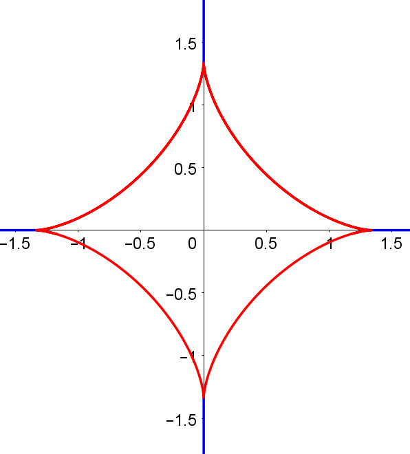
Figure 2: The astroid $\gamma_{4}$ (red) and the four rays obtained by intersecting $H_{1}^{*}$ with the $(x_{1},x_{2})$-plane (blue).

In particular, $H_{1}^{*}$ is the solution of the Björling problem for the curve ${\gamma}_{4}$ and the choice of unit normal field the normal vector to ${\gamma}_{4}$ as a planar curve, see also Remark 8 below.

5 Generalized Henneberg surfaces

We will next search for a $1$-sided, complete, stable minimal surface in $X\colon\Sigma\looparrowright\mathbb{R}^{3}$ with $\Sigma=\overline{\mathbb{C}}\setminus\mathcal{E}$, $\mathcal{E}$ finite and $g(z)=z$. Hence, $I(z)=-1/\overline{z}$, $\widehat{X}=X/\langle I\rangle\colon\Sigma/\langle I\rangle\looparrowright\mathbb{R}^{3}$ is stable and (4) writes

$$f(-1/\overline{z})=-\overline{z^{4}f(z)}.$$ (7)

5.1 General form for $f$

We take a general rational function

$$f(z)=\frac{c}{z^{m+3}}\frac{\prod_{j=1}^{M}(z-a_{j})}{\prod_{j=1}^{N}(z-b_{j})},$$ (8)

where $c,a_{j},b_{j}\in\mathbb{C}^{*}$, $m\in\mathbb{N}$, $M,N\in\mathbb{N}\cup\{0\}$ are to be determined.

Remark 5.

1. Hennerberg’s surface $H_{1}$ has $f(z)=z^{-4}(z^{4}-1)$, hence $c=1$, $m=1$, $N=0$, $M=4$, $\{a_{j}\}=\{\pm 1,\pm i\}$.

2. The zeros of the induced the metric (2) (branch points of the surface) occur precisely at the points $a_{j}$; the ends occur at $0,\infty$ and at the points $b_{j}$ (in particular, both families $\{a_{j}\}_{j},\{b_{j}\}_{j}$ must then come in pairs of antipodal points, see also (12) below).

3. A consequence of the last observation is that when the above rotations in $\mathbb{R}^{3}$ of our surfaces (provided that the Weierstrass data close periods) are not allowed unless the axis of rotation is vertical.

Imposing (7) to (8) we get

$$c(-1)^{m-1+M-N}\overline{z}^{3+m-M+N}\frac{\prod_{j=1}^{M}(1+a_{j}\overline{z})}{\prod_{j=1}^{N}(1+b_{j}\overline{z})}=f(-1/\overline{z})=-\overline{z^{4}f(z)}=-\frac{\overline{c}}{\overline{z}^{m-1}}\frac{\prod_{j=1}^{M}(\overline{z}-\overline{a_{j}})}{\prod_{j=1}^{N}(\overline{z}-\overline{b_{j}})},$$

thus

$$\overline{c}(-1)^{m+M-N}z^{2+2m-M+N}\prod_{j=1}^{M}(1+\overline{a_{j}}z)\prod_{j=1}^{N}(z-b_{j})=c\prod_{j=1}^{M}(z-a_{j})\prod_{j=1}^{N}(1-\overline{b_{j}}z),$$ (9)

from where we deduce that

$$2+2m-M+N=0,$$ (10)

in particular $M-N$ is even. Substituting $z=0$ in (9) we get

$$\overline{c}(-1)^{m}\prod_{j=1}^{N}b_{j}=c\prod_{j=1}^{M}a_{j}.$$ (11)

Using (11), we can rewrite (9) as an equality between monic polynomials in $z$:

$$\prod_{j=1}^{M}\left(\frac{1}{\overline{a_{j}}}+z\right)\prod_{j=1}^{N}(z-b_{j})=\prod_{j=1}^{M}(z-a_{j})\prod_{j=1}^{N}\left(\frac{1}{\overline{b_{j}}}+z\right),$$

from where we deduce that

$$\{a_{1},\dots,a_{M}\}=\{-1/\overline{a_{1}},\dots,-1/\overline{a_{M}}\},\quad\{b_{1},\dots,b_{N}\}=\{-1/\overline{b_{1}},\dots,-1/\overline{b_{N}}\}.$$ (12)

that is, $M,N$ are even, the $a_{j}$ (resp. $b_{j}$) are given by $M/2$ (resp. $N/2$) pairs of antipodal points in $\mathbb{C}^{*}$. Now (10) and (11) give respectively:

$$1+m-\widetilde{M}+\widetilde{N}=0,$$ (13)

$$-\overline{c}\prod_{j=1}^{N/2}\frac{b_{j}}{\overline{b_{j}}}=c\prod_{j=1}^{M/2}\frac{a_{j}}{\overline{a_{j}}}.$$ (14)

5.2 Solving the period problem in the one-ended case: complexity

From (3) and (8) we see that the points where $ds^{2}$ can blow up are $z=0,b_{1},\dots,b_{N}$ and its antipodal points. In order to keep the computations simple, we will assume there are no $b_{j}$’s, i.e. $N=0$ (or equivalently $M/2=m+1$), which reduces the period problem to imposing

$$\overline{\int_{\gamma}g^{2}\omega}=\int_{\gamma}\omega,\qquad\mbox{Re}\int_{\gamma}f\omega=0,$$

where $\gamma=\{|z|=1\}$, or equivalently,

$$\overline{\text{Res}_{0}(g^{2}f)}=-\text{Res}_{0}(f),\quad\text{Im}\,\text{Res}_{0}(gf)=0.$$ (15)

We can simplify (8) to

$$f(z)=\frac{c}{z^{m+3}}\prod_{j=1}^{m+1}(z-a_{j})\left(z+\frac{1}{\overline{a_{j}}}\right),$$ (16)

which satisfies (7) (this is the condition to descend to the quotient as a 1-sided surface, provided that the period problem (15) is solved) if and only if (14) holds, which in this case reduces to

$$-\frac{\overline{c}}{c}=\prod_{j=1}^{m+1}\frac{a_{j}}{\overline{a_{j}}}.$$ (17)

We call

$$P(z):=\prod_{j=1}^{m+1}(z-a_{j})\left(z+\frac{1}{\overline{a_{j}}}\right)=\sum_{h=0}^{2m+2}A_{h}z^{h}.$$ (18)

Thus,

$$\text{Res}_{0}(f)=c\,\text{Res}_{0}(\sum_{h=0}^{2m+2}A_{h}z^{h-m-3})=cA_{m+2},$$

$$\text{Res}_{0}(g^{2}f)=c\,\text{Res}_{0}(\sum_{h=0}^{2m+2}A_{h}z^{h-m-1})=cA_{m},$$

$$\text{Res}_{0}(gf)=c\,\text{Res}_{0}(\sum_{h=0}^{2m+2}A_{h}z^{h-m-2})=cA_{m+1}.$$

Thus, (15) reduces to

$$\overline{cA_{m}}=-cA_{m+2},\quad\text{Im}(cA_{m+1})=0.$$ (19)

Remark 6.

We can assume $|c|=1$ due to the fact that multiplying the Weierstrass form by a positive number does not affect to solving the period problem and just multiplies the resulting surface by a homothety. Similarly, exchanging $c$ by $-c$ does not affect to solving the period problem.

We also write $a_{j}=|a_{j}|e^{i\theta_{j}}$, $\theta_{j}\in\mathbb{R}$. Thus,

$$-a_{j}+\frac{1}{\overline{a_{j}}}=(-|a_{j}|+\frac{1}{|a_{j}|})e^{i\theta_{j}},\quad\frac{a_{j}}{\overline{a_{j}}}=e^{2i\theta_{j}},$$

and so,

$$P(z)=\prod_{j=1}^{m+1}\left(z^{2}+(-|a_{j}|+\frac{1}{|a_{j}|})e^{i\theta_{j}}z-e^{2i\theta_{j}}\right)$$ (20)

Definition 7.

Given $m\in\mathbb{N}$, a list $(c,a_{1},\ldots,a_{m+1})\in\mathbb{S}^{1}\times(\mathbb{C}^{*})^{m+1}$ solving the equations (17),(19) will be called a solution of the period problem with complexity $m$. Note that geometrically, $a_{1},\ldots,a_{m+1}$ are the Gaussian images of the branch points of the resulting surface.

5.3 The case when the $a_{j}$ are the $(2m+2)$-roots of unity

For each complexity $m$, there is a most symmetric configuration that gives rise to a solution of the period problem for that complexity, which we describe next.

Take the $a_{j}$ as the solutions of the equation $a^{2m+2}=1$ (i.e. $|a_{j}|=1$ and $\theta_{j}=\frac{\pi}{m+1}(j-1)$, $j=1,\dots,m+1$). Observe that

$$\prod_{j=1}^{m+1}\frac{a_{j}}{\overline{a_{j}}}=\prod_{j=1}^{m+1}e^{2i\theta_{j}}=e^{2i\sum_{j=1}^{m+1}{\theta}_{j}}=e^{\frac{2\pi i}{m+1}\sum_{j=1}^{m+1}(j-1)}=e^{\frac{2\pi i}{m+1}\frac{m(m+1)}{2}}=e^{i\pi m},$$

hence the validity of (17) is equivalent in this case to

$$c=\pm i^{m-1}.$$ (21)

As for equation (19), note that (20) can be written as

$$P(z)=\prod_{j=1}^{m+1}(z^{2}-e^{2i\theta_{j}})=z^{2m+2}-1,$$

and thus $A_{m}=0$ (because $m>0$), $A_{m+2}=0$ (because $m+2<2m+2$) and $A_{m+1}=0$. In particular, (19) is trivially satisfied for each value of $c\in\mathbb{C}^{*}$. Therefore, the Weierstrass data

$$g(z)=z,\quad\omega=i^{m-1}z^{-m-3}(z^{2m+2}-1)dz,\qquad z\in\mathbb{C}^{*},$$ (22)

give rise to a $1$-sided, complete, stable minimal surface $H_{m}$. For $m=1$ we recover the classical Henneberg’s surface.

5.4 Associated family and the conjugate surface $H_{m}^{*}$.

Since $A_{m}=A_{m+1}=A_{m+2}=0$, the flux vector of $H_{m}$ around the origin in $\mathbb{C}$ vanishes and the Weierstrass form $\Phi=(\phi_{1},\phi_{2},\phi_{3})$ associated to $H_{m}$ is exact. Thus all associated surfaces $\{\widetilde{H}_{m}(\varphi)\ |\ \varphi\in[0,2\pi)\}$ to the orientable cover $\widetilde{H}_{m}=\widetilde{H}_{m}(0)$ of are well-defined. As in the case $m=1$ (see Section 4.2), none of these associated surfaces descends to the $1$-sided quotient, except for $\pm H_{m}$. Let $H_{m}^{*}:=\widetilde{H}_{m}(\pi/2)$ be the conjugate surface to $H_{m}$.

The behavior of $H_{m}$ is very different depending on the parity of $m$. A naive justification of this dependence on the parity of $m$ comes from the fact that the coefficient for $\omega$ changes from $\pm 1$ for $m$ odd to $\pm i$ for $m$ even. A more geometric interpretation of this dependence will be given next.

5.5 The case $m$ odd

If $m\in\mathbb{N}$ is odd, (22) gives $\omega=z^{-m-3}(z^{2m+2}-1)dz$. Although $H_{m}$ has $m+1$ branch points in $\Sigma=\mathbb{P}^{2}\setminus\{[0]\}$ (the classes of the $(2m+2)$-roots of unity under the antipodal map), they are mapped into just two different points in $\mathbb{R}^{3}$: after translating the surface in $\mathbb{R}^{3}$ so that $X(e^{i\frac{\pi}{2(m+1)}})=\vec{0}$ (we are using the notation in (1)), the branch points of $H_{m}$ are mapped to $(0,0,\pm 1)$ and a parameterization of $H_{m}$ in polar coordinates is (compare with (6))

$$X(re^{i\theta})=\left(\begin{array}[]{c}x_{1}\\ x_{2}\\ x_{3}\end{array}\right)=\left(\begin{array}[]{c}\frac{\cos(m{\theta})}{2m}(r^{m}-\frac{1}{r^{m}})-\frac{\cos((m+2)\theta)}{2(m+2)}(r^{m+2}-\frac{1}{r^{m+2}})\\ -\frac{\sin(m{\theta})}{2m}(r^{m}-\frac{1}{r^{m}})-\frac{\sin((m+2)\theta)}{2(m+2)}(r^{m+2}-\frac{1}{r^{m+2}})\\ \frac{\cos((m+1)\theta)}{m+1}(r^{m+1}+\frac{1}{r^{m+1}})\end{array}\right).$$ (23)

$X$ maps the unit circle into the vertical segment $\{(0,0,t)|\,t\in[-1,1]\}$. $\theta\in[0,2\pi]\mapsto X(e^{i\theta})$ bounces between the two branch points of $H_{m}$, and the complement of this closed segment in the $x_{3}$-axis is not contained in $H_{m}$. $H_{m}\cap\{x_{3}=0\}$ consists of an equiangular system of $m+1$ straight lines passing through the origin (the images by $X$ of the straight lines of arguments ${\theta}=\frac{\pi/2+k\pi}{m+1}$, $k=0,\ldots,m$ in polar coordinates), see Figure 4 right for $H_{3}$.

5.6 The case $m$ even

If $m$ is even (and non-zero), (22) produces $\omega=i\,z^{-m-3}(z^{2m+2}-1)dz$. In this case, a parametrization of $H_{m}$ in polar coordinates is

$$X(re^{i\theta})=\left(\begin{array}[]{c}x_{1}\\ x_{2}\\ x_{3}\end{array}\right)=\left(\begin{array}[]{c}-\frac{\sin(m\theta)}{2m}\left(r^{m}+\frac{1}{r^{m}}\right)+\frac{\sin((m+2)\theta)}{2(m+2)}\left(r^{m+2}+\frac{1}{r^{m+2}}\right)\\ -\frac{\cos(m{\theta})}{2m}\left(r^{m}+\frac{1}{r^{m}}\right)-\frac{\cos((m+2)\theta)}{2(m+2)}\left(r^{m+2}+\frac{1}{r^{m+2}}\right)\\ \frac{\sin((m+1)\theta)}{m+1}(\frac{1}{r^{m+1}}-r^{m+1})\end{array}\right).$$ (24)

$X$ maps the unit circle $\{r=1\}$ into a certain hypocycloid contained in the plane $\{x_{3}=0\}$, as we will explain next.

A hypocycloid of inner radius $r>0$ and outer radius $R>r$ is the planar curve traced by a point on a circumference of radius $r$ which is rolling along the interior of another circumference (which is fixed) of radius $R$. It can be parametrized by $\alpha(t)=(x(t),y(t))$, $t\in\mathbb{R}$, where

$$x(t)=-(R-r)\sin t+r\sin\left(\frac{R-r}{r}t\right),\qquad y(t)=-(R-r)\cos t-r\cos\left(\frac{R-r}{r}t\right).$$

Using (24), we deduce that the image by $X$ of the unit circle $\mathbb{S}^{1}\subset\mathbb{C}$ has the following parametrization:

$$\theta\in[0,2\pi)\mapsto X(e^{i\theta})=\left(\begin{array}[]{c}-\frac{\sin(m\theta)}{m}+\frac{\sin((m+2)\theta)}{m+2}\\ -\frac{\cos(m\theta)}{m}-\frac{\cos(m+2)\theta}{m+2}\\ 0\end{array}\right).$$ (25)

From (25) we deduce that, up to the reparametrization $t=m\theta$, $X(\mathbb{S}^{1})$ is the hypocycloid of inner radius $r=\frac{1}{m+2}$ and outer radius $R=\frac{2m+2}{m(m+2)}$, which has exactly $m+1$ cusps. These cusp points are the images by $X$ of the $m+1$ branch points of $H_{m}$. In particular, $H_{m}$ is the unique minimal surface obtained as solution of the Björling problem for the hypocycloid of $m+1$ cusps (this number of cusps is any odd positive integer, at least three), inner radius $r=\frac{1}{m+2}$ and outer radius $R=\frac{2m+2}{m(m+2)}$, when we take as normal vector field $\eta$ (see Section 3 for the notation) the normal vector to the hypocycloid as a planar curve.

We depict this planar curve in the simplest cases $m=2,4,6$ in Figure 3 in red.

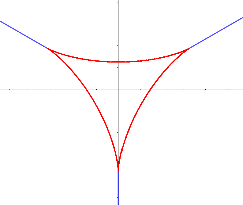
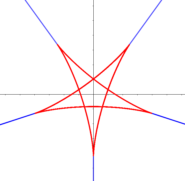
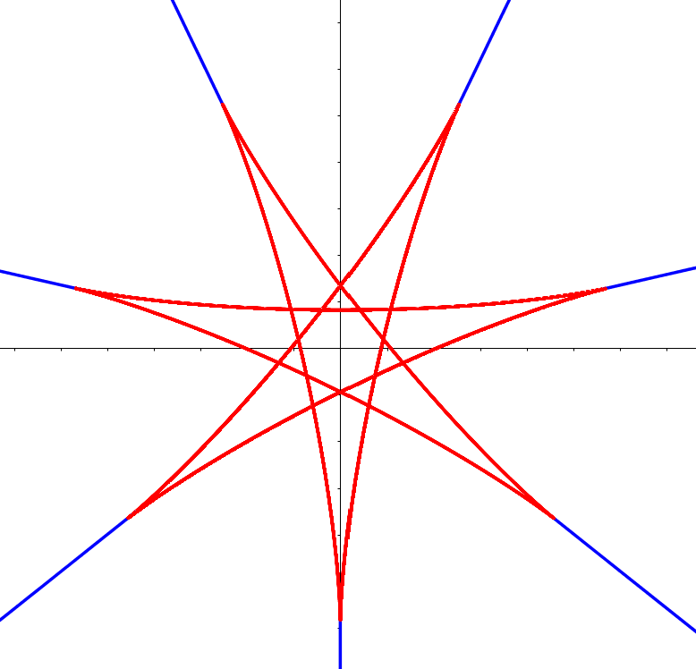
Figure 3: The intersection of $H_{m}$ (with $m>0$ even) with $\{x_{3}=0\}$ consists of a hypocycloid with $m+1$ cusps (in red) together with half-lines $\{tp\ |\ t\geq 1\}$ that start from each of these cusp points $p$. Left: $H_{2}\cap\{x_{3}=0\}$, where the branch points have coordinates $(0,-\frac{3}{4},0),(-\frac{3\sqrt{3}}{8},\frac{3}{8},0),(\frac{3\sqrt{3}}{8},\frac{3}{8},0)$. Center: $H_{4}\cap\{x_{3}=0\}$, Right: $H_{6}\cap\{x_{3}=0\}$.

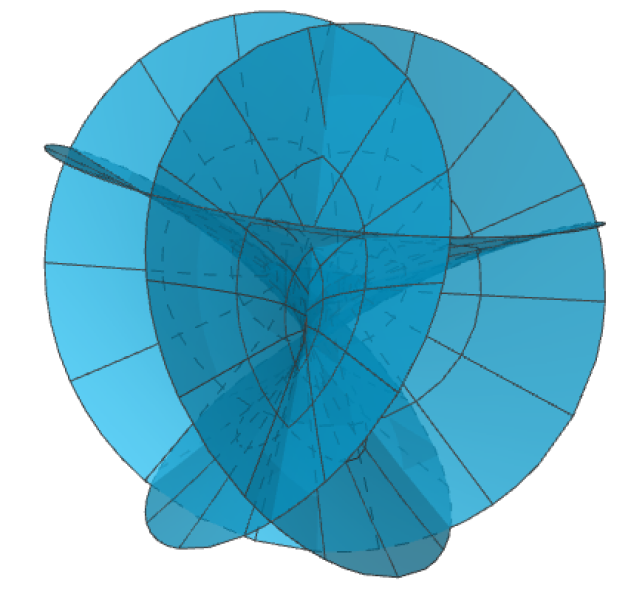
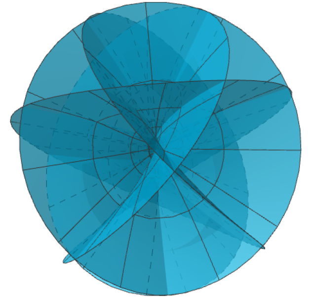
Figure 4: Left: $H_{2}$. Right: $H_{3}$.

5.7 Revisiting the case $m$ odd: $H_{m}^{*}$ as a solution of a Björling problem for a hypocycloid

Using the Weierstrass formula (1), it can be easily seen that the conjugate surface $H_{m}^{*}$ of $H_{m}$ with odd $m$ can be parameterized in polar coordinates $z=re^{i{\theta}}$ by $X^{*}(re^{i{\theta}})$ given by the same formula as the right-hand-side of (24). $X^{*}(\mathbb{S}^{1})$ parameterizes a hypocycloid ${\gamma}_{2m+2}$ with inner radius $r=\frac{1}{m+2}$ and outer radius $R=\frac{2m+2}{m(m+2)}$. Since

$$\frac{R}{r}=\frac{2m+2}{m},$$

we deduce that ${\gamma}_{2m+2}$ has $2m+2$ cusps. Observe that $2m+2$ is a positive multiple of $4$ because $m$ is odd; and conversely, every positive multiple of $4$ can be written as $2m+2$ for a unique $m\in\mathbb{N}$ odd. This tells us that for any $m\in\mathbb{N}$ odd, $H^{*}_{m}$ is the unique solution to the Björling problem for the hypocycloid ${\gamma}_{2m+2}$, when we take as normal vector field $\eta$ the normal vector to ${\gamma}_{2m+2}$ as a planar curve.

Remark 8.

1. In the particular case of a hypocycloid of 4 cusps (called astroid), we recover the conjugate surface $H_{1}^{*}$ of the classical Henneberg surface. This result was described by Odehnal [6], who also studied the Björling problem for an hypocycloid ${\gamma}_{3}$ of three cusps from the viewpoint of algebraic surfaces.

2. We have described the minimal surfaces obtained as the solution of a Björling problem over a hypocycloid if the number of its cusps is either any given odd number or a multiple of four. The case that remains is when the hypocycloid has $4k+2$ cusps, $k\in\mathbb{N}$. The corresponding solution to this Björling problem can be also explicitly described by the parametrization (24), now with a parameter $m\in\mathbb{Q}$. Namely, if we choose $m$ to be of the form $m=\frac{1}{2k}$, $k\in\mathbb{N}$, inner radius $r=\frac{1}{m+2}$ and outer radius $R=\frac{2m+2}{m(m+2)}$, then

   $$\frac{R}{r}=\frac{2m+2}{m}=4k+2,$$

   which ensures that the complete branched minimal surface $H_{\frac{1}{2k}}=X(\mathbb{C}\setminus\{0,\infty\})$ (here $X$ is given by (24)) is symmetric by reflection in the $(x_{1},x_{2})$-plane), and $X(\mathbb{S}^{1})$ is a hypocycloid with $4k+2$ cusps. $H_{\frac{1}{2k}}$ does not descend to a 1-sided quotient.

5.8 Isometries of $H_{m}$

As expected, the isometry group of $H_{m}$ depends on whether $m$ is even or odd.

Suppose firstly that $m$ is odd. In this case, (23) gives:

1. The reflection of the $z$-plane about the imaginary axis, $re^{i\theta}\mapsto re^{i(\pi-\theta)}$, produces via $X$ the reflectional symmetry about the $(x_{2},x_{3})$-plane in $H_{m}$.

2. The rotation $re^{i\theta}\mapsto re^{i({\theta}+\pi+\frac{\pi}{m+1})}$ of angle $\pi+\frac{\pi}{m+1}$ about the origin in the $z$-plane, gives that $H_{m}$ is symmetric under the rotation of angle $\frac{\pi}{m+1}$ about the $x_{3}$-axis composed by a reflection in the $(x_{1},x_{2})$-plane.

(O1), (O2) generate a subgroup of the extrinsic isometry group $\text{Iso}(H_{m})$ of $H_{m}$, isomorphic to the dihedral group $D_{2m+2}$.

Now assume that $m$ is even. Using (24), we obtain:

1. The reflection $re^{i\theta}\mapsto re^{i(\pi-\theta)}$ of the $z$-plane about the imaginary axis produces via $X$ the reflectional symmetry about the $(x_{2},x_{3})$-plane in $H_{m}$ (this is a common feature of both the odd and even cases).

2. The rotation $re^{i\theta}\mapsto re^{i({\theta}+\frac{2\pi}{m+1})}$ of angle $\frac{2\pi}{m+1}$ about the origin in the $z$-plane, gives that $H_{m}$ is symmetric under the rotation of angle $\frac{2\pi}{m+1}$.

3. The antipodal map $re^{i\theta}\mapsto re^{i({\theta}+\pi)}$ in the $z$-plane, produces a reflectional symmetry of $H_{m}$ with respect to the $(x_{1},x_{2})$-plane.

(E1), (E2), (E3) generate a subgroup of $\text{Iso}(H_{m})$ isomorphic to the group $D_{m+1}\times\mathbb{Z}_{2}$.

Repeating the argument in the proof of Lemma 4, we now deduce the following.

Lemma 9.

Regardless of the parity of $m$, these are all the (intrinsic) isometries of $H_{m}$.

6 Moduli spaces of examples with a given complexity

Our next goal is to analyze the structure of the family of solutions of the period problem with a given complexity in the sense of Definition 7. For $m=1$, we will obtain uniqueness of the Henneberg surface $H_{1}$. This uniqueness is a special feature of the case $m=1$, since continuous families of examples for complexities $m\geq 2$ can be produced.

We define the function $R\colon(0,\infty)\to(0,\infty)$, $R(r)=r-\frac{1}{r}$.

6.1 Solutions with complexity $m=1$

Since $m=1$, solving the period problem (19) descending to the 1-sided quotient reduces to solving

$$\overline{cA_{1}}=-cA_{3},\quad\text{Im}(cA_{2})=0,\qquad-\frac{\overline{c}}{c}=\frac{a_{1}}{\overline{a_{1}}}\frac{a_{2}}{\overline{a_{2}}}.$$ (26)

Suppose that a list $(c,a_{1},a_{2})\in\mathbb{S}^{1}\times(\mathbb{C}^{*})^{2}$ is a solution of the 1-sided period problem, with associated branched minimal immersion $X$. Recall that $g(z)=z$ is its Gauss map. The list that gives rise to $H_{1}$ (Henneberg) is $(\pm 1,1,i)$.

Remark 10.

Since rotations of our surfaces are not allowed unless the rotation axis is vertical (see Remark 5), we we can assume $a_{1}\in\mathbb{R}^{+}$ from now on, although we cannot assume $a_{1}=1$.

Write $a_{1},a_{2}$ in polar coordinates as $a_{1}=r_{1}$, $a_{2}=r_{2}e^{i\theta_{2}}$, $r_{1},r_{2}>0$, ${\theta}_{2}\in[0,2\pi)$. (18) can be written as

$$P(z) = z^{4}-\left[R(r_{1})+R(r_{2})e^{i{\theta}_{2}}\right]z^{3}-\left[1+e^{2i\theta_{2}}-R(r_{1})R(r_{2})e^{i{\theta}_{2}}\right]z^{2}$$

$$+\left[R(r_{1})e^{2i{\theta}_{2}}+R(r_{2})e^{i{\theta}_{2}}\right]z+e^{2i{\theta}_{2}},$$

hence

$$A_{1} = R(r_{1})e^{2i{\theta}_{2}}+R(r_{2})e^{i{\theta}_{2}},$$ (27)

$$A_{2} = -\left[1+e^{2i\theta_{2}}-R(r_{1})R(r_{2})e^{i{\theta}_{2}}\right],$$ (28)

$$A_{3} = -\left[R(r_{1})+R(r_{2})e^{i{\theta}_{2}}\right].$$ (29)

Writing $c=e^{i{\beta}}$, we have

$$\overline{cA_{1}}+cA_{3} = R(r_{1})\left[e^{-i({\beta}+2{\theta}_{2})}-e^{i{\beta}}\right]+R(r_{2})\left[e^{-i({\beta}+{\theta}_{2})}-e^{i({\beta}+{\theta}_{2})}\right]$$ (30)

$$= R(r_{1})e^{-i{\theta}_{2}}\left[e^{-i({\beta}+{\theta}_{2})}-e^{i({\beta}+{\theta}_{2})}\right]-2R(r_{2})\sinh(i({\beta}+{\theta}_{2}))$$

$$= -2e^{-i{\theta}_{2}}R(r_{1})\sinh(i({\beta}+{\theta}_{2}))-2iR(r_{2})\sin({\beta}+{\theta}_{2})$$

$$= -2i\left[R(r_{1})e^{-i{\theta}_{2}}+R(r_{2})\right]\sin({\beta}+\theta_{2}),$$

$$cA_{2} = -e^{i{\beta}}\left(1+e^{2i\theta_{2}}\right)+R(r_{1})R(r_{2})e^{i({\beta}+{\theta}_{2})}$$ (31)

$$= -e^{i({\beta}+{\theta}_{2})}\left(e^{-i{\theta}_{2}}+e^{i{\theta}_{2}}\right)+R(r_{1})R(r_{2})e^{i({\beta}+{\theta}_{2})}$$

$$= -\left[2\cosh(i{\theta}_{2})-R(r_{1})R(r_{2})\right]e^{i({\beta}+{\theta}_{2})}$$

$$= -\left[2\cos{\theta}_{2}-R(r_{1})R(r_{2})\right]e^{i({\beta}+{\theta}_{2})}.$$

A list $(c,a_{1},a_{2})$ solves the period problem if and only if the right-hand-side of (30) vanishes and the right-hand-side of (31) is real.

The third equation in (26) reduces to

$$e^{2i({\beta}+{\theta}_{2})}=-1.$$ (32)

Theorem 11.

The Henneberg surface $H_{1}$ is the only surface with $m=1$ that solves the period problem and descends to a 1-sided quotient.

Proof.

By the above arguments, the right-hand-side of (30) vanishes, the right-hand-side of (31) is real and (32) holds.

(32) implies that $\sin({\beta}+{\theta}_{2})=\pm 1$. Since the right-hand-side of (30) vanishes, we have

$$R(r_{1})e^{-i{\theta}_{2}}+R(r_{2})=0.$$ (33)

We have two possibilities:

• $r_{1}=1$. Thus (33) implies $r_{2}=1$. From, (32) we have ${\beta}+{\theta}_{2}\equiv\pi/2\text{ mod }\pi$ and from (31) we have $\cos{\theta}_{2}=0$, thus ${\theta}_{2}=\pi/2$ or ${\theta}_{2}=3\pi/2$. This gives the lists $(1,1,i)$, $(-1,1,i)$, $(1,1,-i)$ and $(-1,1,-i)$. All of them give raise to the Henneberg surface.

• $r_{1}\neq 1$. This implies $e^{-i{\theta}_{2}}=-\frac{R(r_{2})}{R(r_{1})}$, which is real. Hence $e^{-i{\theta}_{2}}=\pm 1$. As the function $r\mapsto R(r)$ is injective, this implies $r_{1}=r_{2}$ and ${\theta}_{2}=\pi$ or $r_{2}=1/r_{1}$ and ${\theta}_{2}=0$. Since the right-hand-side of (31) is real and (32) holds, $2\cos{\theta}_{2}-R(r_{1})R(r_{2})=0$. But in both cases $2\cos{\theta}_{2}-R(r_{1})R(r_{2})$ does not vanish. Hence this possibility cannot occur.

∎

6.2 Solutions with complexity $m=2$

Suppose that a list $(c=e^{i{\beta}},a_{1}=r_{1},a_{2}=r_{2}e^{i{\theta}_{2}},a_{3}=r_{3}e^{i{\theta}_{3}})\in\mathbb{S}^{1}\times\mathbb{R}^{+}\times(\mathbb{C}^{*})^{2}$ is a solution of the period problem with 1-sided quotient and associated branched minimal immersion $X$. The list that gives rise to $H_{2}$ is $(\pm i,1,e^{i\pi/3},e^{2i\pi/3})$.

Solving the period problem with 1-sided quotient is equivalent to solving

$$\overline{cA_{2}}=-cA_{4},\quad\text{Im}(cA_{3})=0,\quad-\frac{\overline{c}}{c}=\frac{a_{2}}{\overline{a_{2}}}\frac{a_{3}}{\overline{a_{3}}}$$ (34)

The third equation in (34) reduces to

$$e^{2i({\beta}+{\theta}_{2}+{\theta}_{3})}=-1.$$ (35)

(18) can be written as

$$P(z)=z^{6}+A_{5}z^{5}+A_{4}z^{4}+A_{3}z^{3}+A_{2}z^{2}+A_{1}z+A_{0},$$

where

$$A_{2} = e^{2i({\theta}_{2}+{\theta}_{3})}+e^{2i{\theta}_{2}}+e^{2i{\theta}_{3}}-R(r_{1})R(r_{2})e^{i({\theta}_{2}+2{\theta}_{3})}-R(r_{1})R(r_{3})e^{i(2{\theta}_{2}+{\theta}_{3})}$$ (36)

$$-R(r_{2})R(r_{3})e^{i({\theta}_{2}+{\theta}_{3})},$$

$$A_{3} = \mbox{}2\textstyle{\left[R(r_{2})\cos{\theta}_{3}+R(r_{3})\cos{\theta}_{2}+R(r_{1})\cos({\theta}_{2}-{\theta}_{3})-\frac{1}{2}R(r_{1})R(r_{2})R(r_{3})\right]}e^{i({\theta}_{2}+{\theta}_{3})},\quad$$ (37)

$$A_{4} = -(1+e^{2i{\theta}_{2}}+e^{2i{\theta}_{3}})+R(r_{1})R(r_{2})e^{i{\theta}_{2}}+R(r_{1})R(r_{3})e^{i{\theta}_{3}}+R(r_{2})R(r_{3})e^{i({\theta}_{2}+{\theta}_{3})}.$$ (38)

Thus,

$$\overline{cA_{2}}+cA_{4} = 2e^{-i[\beta+2({\theta}_{2}+{\theta}_{3})]}F,$$ (39)

$$cA_{3} = \pm 2iG$$ (40)

where

$$F = \textstyle{e^{2i{\theta}_{3}}+\left[2\cos{\theta}_{2}-R(r_{1})R(r_{2})\right]e^{i{\theta}_{2}}-R(r_{3})\left[R(r_{1})+R(r_{2})e^{i{\theta}_{2}}\right]e^{i{\theta}_{3}},}$$ (41)

$$G = \textstyle{R(r_{2})\cos{\theta}_{3}+R(r_{3})\cos{\theta}_{2}+R(r_{1})\cos({\theta}_{2}-{\theta}_{3})-\frac{1}{2}R(r_{1})R(r_{2})R(r_{3}).}$$ (42)

Remark 12.

1. From (42) we deduce that $G$ is real, hence the condition $\text{Im}(cA_{3})=0$ only holds if and only if $G=0$. We deduce that a list $(c,a_{1},a_{2},a_{3})$ solves the 1-sided period problem if and only if (35) holds and $F=G=0$.

2. The expression (41) is symmetric in $(r_{2},{\theta}_{2}),(r_{3},{\theta}_{3})$. This can be deduced from the symmetry of $A_{2},A_{4}$, or directly checked by using the equality

   $$e^{2i{\theta}_{j}}=2\cos{\theta}_{j}e^{i{\theta}_{j}}-1,$$ (43)

   which transforms (41) into

   $$F=(1+e^{2i{\theta}_{2}}+e^{2i{\theta}_{3}})-R(r_{1})\sum_{j=2}^{3}R(r_{j})e^{i{\theta}_{j}}-R(r_{2})R(r_{3})e^{i({\theta}_{2}+{\theta}_{3})}.$$ (44)

Lemma 13.

If $F=0$, then the coefficient of $R(r_{1})$ in (44) is non-zero.

Proof.

Suppose $R(r_{2})e^{i{\theta}_{2}}+R(r_{3})e^{i{\theta}_{3}}=0$. This leads to one of the following two possibilities: (a) $e^{i{\theta}_{2}}=e^{i{\theta}_{3}}$ and $R(r_{2})=-R(r_{3})$ or else (b) $e^{i{\theta}_{2}}=-e^{i{\theta}_{3}}$ and $R(r_{2})=R(r_{3})$. (a) implies $r_{3}=1/r_{2}$ and thus, (44) gives $F=1+e^{2i{\theta}_{2}}(\frac{1}{r_{2}^{2}}+r_{2}^{2})$. (b) implies $r_{2}=r_{3}$ and (44) gives the same expression for $F$. In any case, we deduce from $F=0$ that $e^{2i{\theta}_{2}}$ is real negative, hence $\frac{r_{2}^{2}}{r_{2}^{4}+1}=-e^{2i{\theta}_{2}}=1$. This is impossible, since the function $x>0\mapsto\frac{x}{1+x^{2}}$ has a unique maximum at $x=1$ with value $1/2$. ∎

The next result describes a one-parameter family of non-trivial examples of complexity $m=2$ different from $H_{2}$.

Proposition 14.

Suppose that a list $(c,a_{1},a_{2},a_{3})$ solves the 1-sided period problem. Then:

1. If $r_{1}=1$, and at least one of $r_{2}$ or $r_{3}$ equals one, then $(c,a_{1},a_{2},a_{3})=(\pm i,1,e^{i\pi/3},e^{2i\pi/3})$ and the example is $H_{2}$.

2. If ${\theta}_{2}+{\theta}_{3}=0$ (mod $\pi$), then $r_{2}=r_{3}$ or $r_{2}=1/r_{3}$ and $(r_{1},r_{2})$ are given by the following functions of ${\theta}_{2}\in(\frac{\pi}{4},\frac{\pi}{3}]\cup[\frac{2\pi}{3},\frac{3\pi}{4}):$

   $$R(r_{1}({\theta}_{2})) = \frac{1}{8\sqrt{2}}\frac{\sqrt{f({\theta}_{2})-3}}{\cos{\theta}_{2}\cos(2{\theta}_{2})}[f({\theta}_{2})+3+4\cos(2{\theta}_{2})],$$ (45)

   $$R(r_{2}({\theta}_{2})) = -\frac{\sqrt{f({\theta}_{2})-3}}{\sqrt{2}},$$ (46)

   or else $(r_{1},r_{2})$ are given by the opposite expressions for both $R(r_{1}({\theta}_{2})),R(r_{2}({\theta}_{2}))$, which exchange $(r_{1},r_{2})$ by $(\frac{1}{r_{1}},\frac{1}{r_{2}})$. Here, $f$ is the function

   $$f({\theta}_{2})=\sqrt{1-8\cos(2{\theta}_{2})-8\cos(4{\theta}_{2})}.$$ (47)

Proof.

If $r_{1}=1$, and at least one of $r_{2}$ or $r_{3}$ equals one, then (44) gives $1+e^{2i{\theta}_{2}}+e^{2i{\theta}_{3}}=0$ and (42) gives $R(r_{2})\cos{\theta}_{3}+R(r_{3})\cos{\theta}_{2}=0$. Since at least one of $r_{2}$ or $r_{3}$ equals one, then at least one of $R_{2}$ or $R_{3}$ equals zero. In fact, both $R_{2}=R_{3}=0$ (because otherwise we get $\cos{\theta}_{2}=0$ or $\cos{\theta}_{3}=0$, which prevents $1+e^{2i{\theta}_{2}}+e^{2i{\theta}_{3}}$ from cancelling), and thus, $r_{2}=r_{3}=1$. In this setting, $1+e^{2i{\theta}_{2}}+e^{2i{\theta}_{3}}=0$ leads to $(c,a_{1},a_{2},a_{3})=(\pm i,1,e^{i\pi/3},e^{2i\pi/3})$, which proves item 1.

Now assume ${\theta}_{2}+{\theta}_{3}=0$. Then (44),(42) give respectively

$$1+2\cos(2{\theta}_{2})-R(r_{2})R(r_{3}) = R(r_{1})[R(r_{2})e^{i{\theta}_{2}}+R(r_{3})e^{-i{\theta}_{2}}],$$ (48)

$$(R(r_{2})+R(r_{3}))\cos{\theta}_{2}+R(r_{1})\cos(2{\theta}_{2}) = \frac{1}{2}R(r_{1})R(r_{2})R(r_{3}).$$ (49)

Observe that $R(r_{1})$ cannot vanish by Lemma 13 (another reason is that otherwise, (49) gives $\cos{\theta}_{2}=0$, and (48) gives $-1-R(r_{2})R(r_{3})=0$ which is absurd). From (48) we deduce that $R(r_{2})e^{i{\theta}_{2}}+R(r_{3})e^{-i{\theta}_{2}}$ is real. This implies that $[R(r_{2})-R(r_{3})]\sin{\theta}_{2}=0$. We claim that $\sin{\theta}_{2}\neq 0$; otherwise ${\theta}_{2}\equiv 0$ (mod $\pi$) and (48),(49) give the system

$$3-R(r_{2})R(r_{3}) = \pm R(r_{1})[R(r_{2})+R(r_{3})],$$

$$R(r_{1})\pm(R(r_{2})+R(r_{3})) = \frac{1}{2}R(r_{1})R(r_{2})R(r_{3}),$$

(with the same choice for signs), which can be easily seen not to have solutions.

Thus, $\sin{\theta}_{2}\neq 0$ hence $R(r_{2})=R(r_{3})$ and $r_{2}=r_{3}$. In this setting, (48),(49) reduce to

$$1+2\cos(2{\theta}_{2})-R(r_{2})^{2} = 2R(r_{1})R(r_{2})\cos{\theta}_{2},$$ (50)

$$2R(r_{2})\cos{\theta}_{2}+R(r_{1})\cos(2{\theta}_{2}) = \frac{1}{2}R(r_{1})R(r_{2})^{2}.$$ (51)

If we assume ${\theta}_{2}+{\theta}_{3}=\pi$, then (44),(42) give respectively

$$1+2\cos(2{\theta}_{2})+R(r_{2})R(r_{3}) = R(r_{1})[R(r_{2})e^{i{\theta}_{2}}-R(r_{3})e^{-i{\theta}_{2}}],$$ (52)

$$(-R(r_{2})+R(r_{3}))\cos{\theta}_{2}-R(r_{1})\cos(2{\theta}_{2}) = \frac{1}{2}R(r_{1})R(r_{2})R(r_{3}).$$ (53)

Again, $R(r_{1})$ can not vanish due to Lemma 13. From (52) we deduce that $R(r_{2})e^{i{\theta}_{2}}-R(r_{3})e^{-i{\theta}_{2}}$ is real. This implies that $[R(r_{2})+R(r_{3})]\sin{\theta}_{2}=0$. We claim that $\sin{\theta}_{2}\neq 0$; otherwise ${\theta}_{2}\equiv 0$ (mod $\pi$) and (52),(53) give the system

$$3+R(r_{2})R(r_{3}) = \pm R(r_{1})[R(r_{2})-R(r_{3})],$$

$$-R(r_{1})\pm(-R(r_{2})+R(r_{3})) = \frac{1}{2}R(r_{1})R(r_{2})R(r_{3}),$$

(with the same choice for signs), which again has no solutions. Thus, $\sin{\theta}_{2}\neq 0$ hence $R(r_{2})=-R(r_{3})$ and $r_{2}=1/r_{3}$. In this setting, (48),(49) reduce again to (50) and (51).

The system (50),(51) has two equations and three unknowns $r_{1},r_{2},{\theta}_{2}$. Next we describe its solutions. Consider the function $f$ given by (47). Then,

$$f(\pi-{\theta}_{2})=f({\theta}_{2}),\mbox{ for each }{\theta}_{2},\quad f({\theta}_{2,0})=0=f(\pi-{\theta}_{2,0}),$$

where ${\theta}_{2,0}=\frac{1}{2}\cot^{-1}\left(\frac{9}{\sqrt{32\sqrt{10}+95}}\right)\sim 0.499841$, and the domain of $f$ is $[{\theta}_{2,0},\pi-{\theta}_{2,0}]+\pi\mathbb{Z}$. The set $\{{\theta}_{2}\in[{\theta}_{2,0},\pi-{\theta}_{2,0}]\ |\ f({\theta}_{2})\geq 3\}$ equals $A:=[\frac{\pi}{4},\frac{\pi}{3}]\cup[\frac{2\pi}{3},\frac{3\pi}{4}]$.

The unique solution $(r_{1},r_{2})$ to the system (50),(51) as a function of ${\theta}_{2}$ is given by (45), (46) and the opposite expressions for both $R(r_{1}({\theta}_{2})),R(r_{2}({\theta}_{2}))$, which exchange $(r_{1},r_{2})$ by $(\frac{1}{r_{1}},\frac{1}{r_{2}})$. ∎

6.2.1 The one-parameter family of examples in item 2 of Proposition 14

Observe that the map ${\theta}_{2}\in(\frac{\pi}{4},\frac{\pi}{3}]\mapsto\pi-{\theta}_{2}\in[\frac{2\pi}{3},\frac{3\pi}{4})$ is a diffeomorphism. Using the notation in item 2 of Proposition 14, for each ${\theta}_{2}\in(\frac{\pi}{4},\frac{\pi}{3}]$, we have

$$R(r_{1}(\pi-{\theta}_{2}))=-R(r_{1}({\theta}_{2})),\qquad R(r_{2}(\pi-{\theta}_{2})))=R(r_{2}({\theta}_{2})).$$ (54)

Each of these lists with ${\theta}_{2}\in(\frac{\pi}{4},\frac{\pi}{3}]\cup[\frac{2\pi}{3},\frac{3\pi}{4})$ solves the 1-sided period problem, hence it defines a non-orientable, branched minimal surface $H({\theta}_{2})$. Furthermore, (54) implies that

$$r_{1}(\pi-{\theta}_{2})=\frac{1}{r_{1}({\theta}_{2})},\qquad r_{2}(\pi-{\theta}_{2})=r_{2}({\theta}_{2}).$$ (55)

We claim the surfaces $H({\theta}_{2})$ and $H(\pi-{\theta}_{2})$ are congruent. To see this, note that the set of points $\{a_{j},-1/\overline{a_{j}}\ :\ j=1,2,3\}$ that defines $f$ through (16) and generates the surface $H({\theta}_{2})$, is:

$$\left\{r_{1},\frac{-1}{r_{1}},r_{2}e^{i\theta_{2}},\frac{1}{r_{2}}e^{i(\pi+\theta_{2})},r_{2}e^{-i\theta_{2}},\frac{1}{r_{2}}e^{i(\pi-\theta_{2})}\right\}.$$ (56)

The analogous set of points for the surface $H(\pi-{\theta}_{2})$ is given through (55):

$$\left\{\frac{1}{r_{1}},-r_{1},-r_{2}e^{-i\theta_{2}},\frac{1}{r_{2}}e^{-i\theta_{2}},-r_{2}e^{-i\theta_{2}},\frac{1}{r_{2}}e^{i\theta_{2}}\right\},$$

which is up to sign the set described in (56). Therefore, the function $f$ defined by equation (16) and the corresponding function $\widetilde{f}$ defined by the same formula for the surface $H(\pi-{\theta}_{2})$ are related by $\widetilde{f}(-z)=-f(z)$, for each $z\in\mathbb{C}$. Using that $\omega=f\,dz$ and $\widetilde{\omega}=\widetilde{f}\,dz$ define, via the Weierstrass representation (1), related branched minimal immersions $X=(x_{1},x_{2},x_{3})$ for $H({\theta}_{2})$ and $\widetilde{X}=(\widetilde{x}_{1},\widetilde{x}_{2},\widetilde{x}_{3})$ for $H(\pi-{\theta}_{2})$, we get that $H({\theta}_{2})$ and $H(\pi-{\theta}_{2})$ are congruent.

In the sequel, we will reduce our study to the family $\{H({\theta}_{2})\ |\ {\theta}_{2}\in(\frac{\pi}{4},\frac{\pi}{3}]\}$. From (45), (46) we have

$$\lim_{{\theta}_{2}\to\pi/3^{-}}R(r_{1}({\theta}_{2}))=\lim_{{\theta}_{2}\to\pi/3^{-}}R(r_{2}({\theta}_{2}))=0,$$

which implies that

$$\lim_{{\theta}_{2}\to\pi/3^{-}}H({\theta}_{2})=H_{2}.$$

We next identify the limit (after rescaling) of the surfaces $H({\theta}_{2})$ as ${\theta}_{2}\to\pi/4^{+}$. We first observe that

$$\lim_{{\theta}_{2}\to\pi/4^{+}}R(r_{1}({\theta}_{2}))=-\infty,\qquad\lim_{{\theta}_{2}\to\pi/4^{+}}R(r_{2}({\theta}_{2}))=0.$$ (57)

This implies that the branch point $a_{1}=a_{1}({\theta}_{2})$ is tending to zero, hence the limit of $H({\theta}_{2})$ when ${\theta}_{2}\to\pi/4^{+}$ (if it exists) cannot be an example with complexity $m=2$. Intuitively, it is clear than the complexity cannot increase when taking limits (even with different scales), hence by Theorem 11 it is natural to think that the limit of suitable re-scalings of $H({\theta}_{2})$ when ${\theta}_{2}\to\pi/4^{+}$ be $H_{1}$. We next formalize this idea.

Another consequence of (57) is that the list $(c,a_{1},a_{2},a_{3})=(i,r_{1}({\theta}_{2}),r_{2}({\theta}_{2})e^{i{\theta}_{2}},r_{2}({\theta}_{2})e^{-i{\theta}_{2}})$ converges as ${\theta}_{2}\to\pi/4^{+}$ to $(c,a_{1},a_{2},a_{3})=(i,0,e^{i\pi/4},e^{-i\pi/4})$. After applying to $H({\theta}_{2})$ a homothety of ratio $r_{1}({\theta}_{2})>0$ (which shrinks to zero), the Weierstrass data of the shrunk surface $r_{1}({\theta}_{2})H({\theta}_{2})$ is $(g(z)=z,\ r_{1}({\theta}_{2})f(z))$, where $f(z)$ is given by (16). For $z\in\mathbb{C}\setminus\{0\}$ fixed,

$$\begin{array}[]{l}{\displaystyle\lim_{{\theta}_{2}\to\pi/4^{+}}r_{1}({\theta}_{2})f(z)}\stackrel{{\scriptstyle\eqref{2.13}}}{{=}}{\displaystyle\lim_{{\theta}_{2}\to\pi/4^{+}}r_{1}({\theta}_{2})\frac{i}{z^{5}}\prod_{j=1}^{3}(z-a_{j})\left(z+\frac{1}{\overline{a_{j}}}\right)}\\ =\frac{i}{z^{5}}\left(z-e^{i\pi/4}\right)\left(z+e^{i\pi/4}\right)\left(z-e^{-i\pi/4}\right)\left(z+e^{-i\pi/4}\right){\displaystyle\lim_{{\theta}_{2}\to\pi/4^{+}}}(z-r_{1}({\theta}_{2}))\left(r_{1}({\theta}_{2})z+1\right)\\ =\frac{i}{z^{4}}\left(z-e^{i\pi/4}\right)\left(z+e^{i\pi/4}\right)\left(z-e^{-i\pi/4}\right)\left(z+e^{-i\pi/4}\right):=\widehat{f}(z).\end{array}$$

Plugging the Weierstrass data $(g(z)=z\widehat{f}\,dz)$ into (1), we obtain a parametrization of the limit surface of $r_{1}({\theta}_{2})H({\theta}_{2})$ as ${\theta}_{2}\to\pi/4^{+}$ in polar coordinates $z=re^{i{\theta}}$:

$$\widehat{X}(re^{i\theta})=\left(\begin{array}[]{c}\frac{-\sin\theta}{2}(r-\frac{1}{r})+\frac{\sin(3\theta)}{6}(r^{3}-\frac{1}{r^{3}})\vspace{0.2cm}\\ -\frac{\cos\theta}{2}(r-\frac{1}{r})-\frac{\cos(3\theta)}{6}(r^{3}-\frac{1}{r^{3}})\vspace{0.2cm}\\ -\cos\theta\sin\theta(r^{2}+\frac{1}{r^{2}})\end{array}\right).$$ (58)

We claim that this parametrization generates the Henneberg surface $H_{1}$. To see this, observe that if we first perform the change of variables $\theta=\widetilde{\theta}+\pi/4$ and then rotate the surface an angle of $-\frac{\pi}{4}$ around the $x_{3}$-axis, we get

$$\left(\begin{array}[]{ccc}\cos\left(\frac{\pi}{4}\right)&\sin\left(\frac{\pi}{4}\right)&0\\ -\sin\left(\frac{\pi}{4}\right)&\cos\left(\frac{\pi}{4}\right)&0\\ 0&0&1\end{array}\right)\cdot\widehat{X}(re^{i\left(\widetilde{\theta}+\frac{\pi}{4}\right)})=-\left(\begin{array}[]{c}\frac{\cos\widetilde{\theta}}{2}(r-\frac{1}{r})-\frac{\cos(3\widetilde{\theta})}{6}(r^{3}-\frac{1}{r^{3}})\\ -\frac{\sin\widetilde{\theta}}{2}(r-\frac{1}{r})-\frac{\sin(3\widetilde{\theta})}{6}(r^{3}-\frac{1}{r^{3}})\\ \frac{\cos(2\widetilde{\theta})}{2}(r^{2}+\frac{1}{r^{2}})\end{array}\right),$$

which is, up to a sign, the parametrization given in (6) for $H_{1}$.

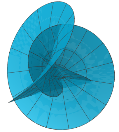
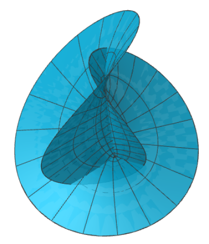
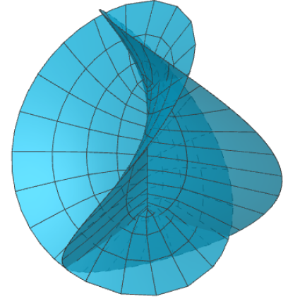
Figure 5: Surfaces generated by the previous lists $(c,a_{1},a_{2},a_{3})=(i,r_{1}({\theta}_{2}),r_{2}({\theta}_{2})e^{i{\theta}_{2}},r_{2}({\theta}_{2})e^{-i{\theta}_{2}})$ with ${\theta}_{2}=1$ (left), ${\theta}_{2}=0.83$ (center), ${\theta}_{2}=0.7854$ (right). The limit of $r_{1}({\theta}_{2})H({\theta}_{2})$ as ${\theta}_{2}\to\pi/4^{+}\sim 0.785398$ is the Henneberg surface $H_{1}$.

6.2.2 Around $H_{2}$ the space of examples with complexity $m=2$ is two-dimensional

Item 2 of Proposition 14 defines a non-compact family of non-orientable, branched minimal surfaces $\{H({\theta}_{2})\ |\ {\theta}_{2}\in(\frac{\pi}{4},\frac{\pi}{3}]\}$ inside the moduli space of examples with complexity $m=2$. Apparently, the space of solutions for this complexity has real dimension 2 (the variables are $r_{1},r_{2},r_{3},{\theta}_{2},{\theta}_{3}$, $F=0$ is a complex condition and $G=0$ is a real condition). We can ensure this at least around $H_{2}$ via the implicit function theorem (this is consistent with item 2 of Proposition 14, since it imposes the extra condition ${\theta}_{2}+{\theta}_{3}=0$ mod $\pi$), as we will show next.

Consider the (smooth) period map given by

$$\begin{array}[]{rccl}P:&(\mathbb{R}^{+})^{3}\times\mathbb{R}^{2}&\longrightarrow&\mathbb{R}^{3}\equiv\mathbb{C}\times\mathbb{R}\\ &((r_{1},r_{2}),(r_{3},{\theta}_{2},{\theta}_{3}))&\longmapsto&(F(r_{1},r_{2},r_{3},{\theta}_{2},{\theta}_{3}),G(r_{1},r_{2},r_{3},{\theta}_{2},{\theta}_{3})),\end{array}$$

where $F,G$ are given by (44), (42) respectively. Given $(r_{1},r_{2})\in(\mathbb{R}^{+})^{2}$, let $P^{r_{1},r_{2}}\colon\mathbb{R}^{+}\times\mathbb{R}^{2}\to\mathbb{R}^{3}$ be the restriction of $P$ to $\{(r_{1},r_{2})\}\times\mathbb{R}^{+}\times\mathbb{R}^{2}$. Then,

$$d(P^{r_{1},r_{2}})_{(r_{3},{\theta}_{2},{\theta}_{3})}\equiv\left(\begin{array}[]{ccc}\displaystyle\frac{\partial\text{Re}(F)}{\partial r_{3}}&\displaystyle\frac{\partial\text{Re}(F)}{\partial{\theta}_{2}}&\displaystyle\frac{\partial\text{Re}(F)}{\partial{\theta}_{3}}\\ \\ \displaystyle\frac{\partial\text{Im}(F)}{\partial r_{3}}&\displaystyle\frac{\partial\text{Im}(F)}{\partial{\theta}_{2}}&\displaystyle\frac{\partial\text{Im}(F)}{\partial{\theta}_{3}}\\ \\ \displaystyle\frac{\partial G}{\partial r_{3}}&\displaystyle\frac{\partial G}{\partial{\theta}_{2}}&\displaystyle\frac{\partial G}{\partial{\theta}_{3}}\\ \\ \end{array}\right).$$ (59)

Recall that the list associated to $H_{2}$ is $(r_{1},r_{2},r_{3},{\theta}_{2},{\theta}_{3})=(1,1,1,\pi/3,2\pi/3)$. Imposing this choice of parameters and computing the determinant of (59) we get

$$d(P^{1,1})_{(1,\pi/3,2\pi/3)}=2\sqrt{3}\neq 0.$$

Thus, the implicit function theorem gives an open neighborhood $U\subset(\mathbb{R}^{+})^{2}$ of $(r_{1},r_{2})=(1,1)$, an open set $W\subset(\mathbb{R}^{+})^{3}\times\mathbb{R}^{2}$ with $(r_{1},r_{2},r_{3},{\theta}_{2},{\theta}_{3})=(1,1,1,\pi/3,2\pi/3)\in W$ and a smooth map $\varphi\colon U\to\mathbb{R}^{3}$ such that all the solutions $(r_{1},r_{2},{\theta}_{1},{\theta}_{2},{\theta}_{3})$ around $(1,1,1,\pi/3,2\pi/3)$ of the equation $P(r_{1},r_{2},{\theta}_{1},{\theta}_{2},{\theta}_{3})=0$ are of the form $({\theta}_{1},{\theta}_{2},{\theta}_{3})=\varphi(r_{1},r_{2})$. By Remark 12(I), the list

$$(c=e^{i{\beta}(r_{1},r_{2})},r_{1},r_{2}e^{i{\theta}_{2}},r_{3}e^{i{\theta}_{3}})$$

with ${\beta}={\beta}(r_{1},r_{2})$ given by (35) solves the 1-sided period problem and so, it defines a $1$-sided branched minimal surface. This produces a 2-parameter deformation of the surface $H_{2}$ in the moduli space of examples with $m=2$ around $H_{2}$, which in turn describes the whole moduli space around $H_{2}$.

Remark 15.

A nice consequence of the classical Leibniz formula for the derivative of a product is a recursive law that gives the coefficients of the polynomial $P(z)$ defined by (18) in terms of the coefficients of the related polynomial for one complexity less. To obtain this recursive law, we first adapt the notation to the complexity:

$$P_{m+1}(z):=\prod_{j=1}^{m+1}(z-a_{j})\left(z+\frac{1}{\overline{a_{j}}}\right)=\sum_{h=0}^{2m+2}A_{m+1,h}z^{h}.$$ (60)

(19) can now be written

$$\overline{cA_{m+1,m}}=-cA_{m+1,m+2},\quad\text{Im}(cA_{m+1,m+1})=0.$$ (61)

We want to find expressions for the above coefficients $A_{m+1,m},A_{m+1,m+2},A_{m+1,m+1}$, depending only on coefficients of the type $A_{m,h}$ (i.e., for one complexity less). Writing $a_{j}=r_{j}e^{i{\theta}_{j}}$ in polar coordinates, observe that

$$P_{m+1}(z):=P_{m}(z)Q_{m+1}(z),\qquad\mbox{where }Q_{m+1}(z)=(z-r_{m+1}e^{i{\theta}_{m+1}})\left(z+\frac{e^{i{\theta}_{m+1}}}{r_{m+1}}\right).$$

Hence for $h\in\{m,m+1,m+2\}$,

$$A_{m+1,h} = \frac{1}{h!}P_{m+1}^{(h)}(0)=\frac{1}{h!}(P_{m}Q_{m+1})^{(h)}(0)=\frac{1}{h!}\sum_{k=0}^{h}\binom{h}{k}P_{m}^{(k)}(0)Q_{m+1}^{(h-k)}(0),$$

where in the last equality we have used Leibniz formula. Since $Q_{m+1}$ is a polynomial of degree two, its derivatives of order three or more vanish. Hence we can reduce the last sum to terms where the index $k$ satisfies $h-k\leq 2$, i.e., $k\in\{h-2,h-1,h\}$ and thus,

$$A_{m+1,h} = \frac{1}{h!}\textstyle{\left[\binom{h}{h-2}P_{m}^{(h-2)}(0)Q_{m+1}^{\prime\prime}(0)+\binom{h}{h-1}P_{m}^{(h-1)}(0)Q_{m+1}^{\prime}(0)+\binom{h}{h}P_{m}^{(h)}(0)Q_{m+1}(0)\right]}$$ (62)

$$= \frac{1}{h!}\textstyle{\left[\frac{h!}{(h-2)!2}P_{m}^{(h-2)}(0)\cdot 2-h\,P_{m}^{(h-1)}(0)R(r_{m+1})e^{i{\theta}_{m+1}}-P_{m}^{(h)}(0)e^{2i{\theta}_{m+1}}\right]}$$

$$= \textstyle{\left[\frac{1}{(h-2)!}P_{m}^{(h-2)}(0)-\frac{1}{(h-1)!}P_{m}^{(h-1)}(0)R(r_{m+1})e^{i{\theta}_{m+1}}-\frac{1}{h!}P_{m}^{(h)}(0)e^{2i{\theta}_{m+1}}\right]}$$

$$= A_{m,h-2}-A_{m,h-1}R(r_{m+1})e^{i{\theta}_{m+1}}-A_{m,h}e^{2i{\theta}_{m+1}},$$

which is the desired recurrence law. (62) can be used to find solutions to (61) for complexity $m=3$ besides the most symmetric example $H_{3}$, but the equations are complicated and we will not give them here.

References

- [1] M. do Carmo and C. K. Peng. Stable complete minimal surfaces in are planes. Bull. Amer. Math. Soc. (N.S.), 1:903–906, 1979. MR0546314, Zbl 442.53013.
- [2] D. Fischer-Colbrie and R. Schoen. The structure of complete stable minimal surfaces in -manifolds of nonnegative scalar curvature. Comm. on Pure and Appl. Math., 33:199–211, 1980. MR0562550, Zbl 439.53060.
- [3] L. Henneberg. Über salche minimalfläche, welche eine vorgeschriebene ebene curve sur geodätishen line haben. Doctoral Dissertation, Eidgenössisches Polythechikum, Zurich, 1875.
- [4] W. H. Meeks III and J. Pérez. Hierarchy structures in finite index cmc surfaces. Work in progress.
- [5] M. Micallef and B. White. The structure of branch points in minimal surfaces and in pseudoholomorphic curves. Ann. of Math., 141(1):35–85, 1995. MR1314031, Zbl 0873.53038.
- [6] B. Odehnal. On algebraic minimal surfaces. KoG, 20:61–78, 2016.
- [7] A. V. Pogorelov. On the stability of minimal surfaces. Soviet Math. Dokl., 24:274–276, 1981. MR0630142, Zbl 0495.53005.
- [8] A. Ros. One-sided complete stable minimal surfaces. J. Differential Geom., 74:69–92, 2006. MR2260928, Zbl 1110.53009.
- [9] J. Tysk. Eigenvalue estimates with applications to minimal surfaces. Pacific J. of Math., 128:361–366, 1987. MR0888524, Zbl 0594.58018.