Folding over Neural Networks

Abstract

Neural networks are typically represented as data structures that are traversed either through iteration or by manual chaining of method calls. However, a deeper analysis reveals that structured recursion can be used instead, so that traversal is directed by the structure of the network itself. This paper shows how such an approach can be realised in Haskell, by encoding neural networks as recursive data types, and then their training as recursion scheme patterns. In turn, we promote a coherent implementation of neural networks that delineates between their structure and semantics, allowing for compositionality in both how they are built and how they are trained.

1 Introduction

Neural networks are graphs whose nodes and edges are organised into layers, generally forming a sequence of layers:

Given input data (on the left), which is propagated through a series of transformations performed by each layer, the final output (on the right) assigns some particular meaning to the input. This process is called forward propagation. To improve the accuracy of neural networks, their outputs are compared with expected values, and the discrepencies are sent back in the reverse direction through each layer to appropriately update their parameters. This is back propagation.

How these notions are typically implemented is highly influenced by object-oriented and imperative programming design, where leading frameworks such as Keras [3] and PyTorch [16] can build on the extensive, existing support for machine learning in their host language. However, the design patterns of these paradigms tend to forgo certain appealing abstractions of neural networks; for example, one could perhaps view the diagram above as a composition of functions as layers, whose overall network structure is described by a higher-order function. Such concepts are more easily captured by functional languages, where networks can be represented as mathematical objects that are amenable to interpretation.

The relationship of neural networks with functional programming has been demonstrated several times, introducing support for compositional and type-safe implementation in various manners [14, 4, 2]. Using Haskell, this paper explores a categorical narrative that offers structure and compositionality in new ways:

• We illustrate how fully connected networks can be expressed as fixed-points of recursive data structures, and their operations of forward and back propagation as patterns of folds and unfolds over these structures. Neural network training (forward then back propagation) is then realised as a composition of fold and unfold (§ 3).

• We generalise our definition of neural networks into their types of layers by using coproducts, and provide an interface for modularly constructing networks using free monads (§ 4).

• We show how neural network training can be condensed into a single fold (§ 5).

We represent the ideas above with structured recursion schemes [9]. By doing so, we create a separation of concern between what the layers of a neural network do from how they comprise the shape of the overall network; this then allows compositionality to be developed in each of these areas individually.

A vast number of neural network architectures are sequentially structured [1, 21, 8]. This paper hence uses fully connected networks [17] as a running example, being simple yet representative of this design. In turn, we believe the ideas presented are transferable to networks with more complex sequential structure, perhaps being sequential across multiple directions; we have tested this with convolutional networks [24] and recurrent networks [12] in particular.

2 Background

We begin by giving the necessary background to the recursion schemes used throughout this paper. First, consider the well-known recursive List type:

⬇

data List a = Nil $|$ Cons a (List a)

Folding and unfolding over a list are then defined as:

⬇

foldr::(a $\rightarrow{}$ b $\rightarrow{}$ b) $\rightarrow{}$ b $\rightarrow{}$ List a $\rightarrow{}$ b

foldr f z Nil = z

foldr f z (Cons x xs) = f x (foldr f z xs)

⬇

unfoldr::(b $\rightarrow{}$ Maybe (a, b)) $\rightarrow{}$ b $\rightarrow{}$ List a

unfoldr f b = case f b of

Just (a, b’) $\rightarrow{}$ Cons a (unfoldr f b’)

Nothing $\rightarrow{}$ Nil

Here, foldr recursively evaluates over a list of type [a] to an output of type b, by iteratively applying an accumulator function f (with some base value z). Conversely, unfoldr recursively builds a list of type [a] from a seed value b, by iteratively applying some generator function g.

2.0.1  Non-recursive functors and fix points

The above useful patterns of recursion can be generalised to work over arbitrary nested data types, by requiring a common structure to recurse over – in particular, as a functor f:

⬇

class Functor f where

fmap :: (k $\rightarrow{}$ l) $\rightarrow{}$ f k $\rightarrow{}$ f l

Additionally, f is required to be non-recursive, and recursion is instead represented abstractly in its type parameter k of f k. The function fmap can then support generic mappings to the recursive structure captured by k.

For example, the standard type List can be converted into a non-recursive functor ListF a:

⬇

data ListF a k = NilF $|$ ConsF a k

instance Functor (ListF a) where

fmap f NilF = NilF

fmap f (ConsF a k) = ConsF a (f k)

which is functorial over the new type parameter k, implicitly representing the recursive occurrence of ListF.

All explicit recursion is then instead relocated to the fixed-point type Fix f:

⬇

newtype Fix f = In (f (Fix f))

out :: Functor f $\Rightarrow{}$ Fix f $\rightarrow{}$ f (Fix f)

out (In f) = f

The constructor In wraps a recursive structure of type f (Fix f) to yield the type Fix f, and the function out deconstructs this to reattain the type f (Fix f). Values of type Fix f hence encode the generic recursive construction of a functor f.

For example, the list [1, 2] in its Fix form would be represented as:

⬇

In (ConsF 1 (In (ConsF 2 (In NilF)))) :: Fix (ListFInt)

As NilF contains no parameter k, it encodes the base case (or least fixed-point) of the structure.

The ideas introduced so far provide us a setting for defining and using recursion schemes; this paper makes use of two in particular: catamorphisms (folds) and anamorphisms (unfolds).

2.0.2  Catamorphisms

A catamorphism, given by the function cata, generalises over folds of lists to arbitrary algebraic data types [11].

⬇

cata :: Functor f $\Rightarrow{}$ (f a $\rightarrow{}$ a) $\rightarrow{}$ Fix f $\rightarrow{}$ a

cata alg = alg $\circ$ fmap (cata alg) $\circ$ out

The argument alg is called an f-algebra or simply algebra, being a function of type f a $\rightarrow{}$ a; this describes how a data structure of type f a is evaluated to an underlying value of type a. The type a is referred to as the algebra’s carrier type.

Informally, cata recursively evaluates a structure of type Fix f down to an output of type a, by unwrapping the constructor of Fix via out, and then interpreting constructors of f with alg.

2.0.3  Anamorphisms

Conversely, an anamorphism, given by ana, generalises over unfolds of lists to arbitrary algebraic data types [13].

⬇

ana :: Functor f $\Rightarrow{}$ (b $\rightarrow{}$ f b) $\rightarrow{}$ b $\rightarrow{}$ Fix f

ana coalg = In $\circ$ fmap (ana coalg) $\circ$ coalg

The argument coalg is called an f-coalgebra or simply coalgebra, being a function of type b $\rightarrow{}$ f b; this describes how a structure of type f b is constructed from an initial value of type b, where b is the carrier type of the coalgebra.

The function ana recursively generates a structure of type Fix f from a seed value of type b, by using coalg to replace occurrences of b with constructors of f, and then wrapping the result with the Fix constructor In.

3 Fully Connected Networks

We now consider how fully connected networks, one of the simplest types of neural networks, can be realised as an algebraic data type for structured recursion to operate over. These consist of a series of layers whose nodes are connected to all nodes in the previous and next layer:

The functor f chosen to represent this structure is the layer type, Layer:

⬇

data Layer k = InputLayer Values $|$ DenseLayer Weights Biases k deriving Functor

type Values = [Double]

type Biases = [Double]

type Weights = [[Double]]

The case InputLayer is the first layer of the network and contains only the network’s initial input Values. This is the base case of the functor.

The case DenseLayer is any subsequent layer (including the output layer), and contains as parameters a matrix Weights and vector Biases which are later used to transform a given input. Its argument k then represents its previous connected layer as a recursive parameter.

Notice that the dimensions of Weights and Biases in fact sufficiently describe a layer’s internal structure:

In the example layer $l$ above, each $j^{th}$ node has a bias value $b_{l}^{j}$, and the edge to the $j^{th}$ node from the previous layer’s $i^{th}$ node has a weight value $w_{l}^{(i,j)}$. Hence, a weight matrix with dimensions $n\times m$ specifies $n$ nodes in the current layer, with each node having $m$ in-degrees. One could make this structure explicit by choosing a more precise type such as vectors [2], but we avoid this for simplicity.

By then incorporating Fix, an instance of a network is represented as a recursive nesting of layers of type Fix Layer. For example, below corresponds to the fully connected network shown at the beginning of § 3:

⬇

fixNetwork :: Fix Layer

fixNetwork = In (DenseLayer $w_{3}$ $b_{3}$ – $l=3,\;\textsf{dims}(w_{3})=2\times 3$

(In (DenseLayer $w_{2}$ $b_{2}$ – $l=2,\;\textsf{dims}(w_{2})=3\times 3$

(In (DenseLayer $w_{1}$ $b_{1}$ – $l=1,\;\textsf{dims}(w_{1})=3\times 2$

(In (InputLayer $a_{0}$))))))   – $l=0,\;\textsf{dims}(a_{0})\,=2$

A comparison can be drawn between the above construction and that of lists, where DenseLayer and InputLayer are analogous to Cons and Nil. Of course, there are less arduous ways of constructing such values, and a monadic interface for doing this is later detailed in § 4.

The type Fix Layer then provides a base for encoding the operations of neural networks – forward and back propagation – as recursion schemes.

3.1 Forward propagation as a catamorphism

The numerous end-user applications that neural networks are well-known for, such as facial recognition [10] and semantic parsing [25], are all done via forward propagation: given unstructured input data, this is propagated through a sequence of transformations performed by each network layer; the final output can then be interpreted meaningfully by humans, for example, as a particular decision or some classification of the input.

One may observe that forward propagation resembles that of a fold: given an input, the layers of a neural network are recursively collapsed and evaluated to an output value (analogous to folding a list whose elements are layers). We can implement this notion using a generalised fold – a catamorphism – over the type Fix Layer; to do so simply requires a suitable algebra to fold with.

An algebra for forward propagation

An algebra, f a $\rightarrow{}$ a, specialised to our context will represent forward propagation over a single layer. The functor f is hence Layer. The choice of carrier type a is [Values], that is, the accumulation of outputs of all previous layers. This gives rise to the following type signature:

⬇

alg${}_{\scriptsize\textsf{fwd}}$ :: Layer [Values] $\rightarrow{}$ [Values]

Defining the case for InputLayer is trivial: a singleton list containing only the initial input $a_{0}$ is passed forward to the next layer.

⬇

alg${}_{\scriptsize\textsf{fwd}}$ (InputLayer $a_{0}$) = $[a_{0}]$

Defining the case for DenseLayer is where any numerical computation is involved:

⬇

alg${}_{\scriptsize\textsf{fwd}}$ (DenseLayer $w_{l}$ $b_{\,l}$ ($a_{l-1}\,$:$\,as$)) = ($a_{l}$ : $a_{l-1}\,$:$\,as$)

where $a_{l}$ = $\sigma(w_{l}*a_{l-1}+b_{l})$

Above, the output $a_{l-1}$ of the previous layer is used as input for the current $l^{th}$ layer, letting the next output $a_{l}$ be computed; this is given by multiplying $a_{l-1}$ with weights $w_{l}$, adding on biases $b_{l}$, and applying some normalization function $\sigma$ (we assume the correct operators $*$ and $+$ for matrices or vectors, given fully in § 0.A.1). The output $a_{l}$ is then prepended to the list of previous outputs.

Having defined forward propagation over a single layer, recursively performing this over an entire neural network is done by applying cata alg${}_{\scriptsize\textsf{fwd}}$ to a value of type Fix Layer, yielding each of its layers’ outputs:

⬇

cata alg${}_{\scriptsize\textsf{fwd}}$ :: Fix Layer $\rightarrow{}$ [Values]

This decoupling of non-recursive logic (alg${}_{\scriptsize\textsf{fwd}}$) from recursive logic (cata) provides a concise description of how a layer transforms its input to its output, without concerning the rest of the network structure.

3.1.1  A better algebra for forward propagation

The initial input to a neural network is currently stored as an argument of the InputLayer constructor:

⬇

– currently

data Layer k = InputLayer Values $|$ DenseLayer Weights Biases k

However, this design is somewhat simplistic. Rather, a neural network should be able to exist independently of its input value like so:

⬇

data Layer k = InputLayer $|$ DenseLayer Weights Biases k

and have its input be provided externally instead. To implement this, we will have alg${}_{\scriptsize\textsf{fwd}}$ evaluate a layer to a continuation of type Values $\rightarrow{}$ [Values] that awaits an input before performing forward propagation:

⬇

alg${}_{\scriptsize\textsf{fwd}}$ :: Layer (Values $\rightarrow{}$ [Values]) $\rightarrow{}$ (Values $\rightarrow{}$ [Values])

In the case of InputLayer, this returns a function that wraps some provided initial input into a singleton list:

⬇

alg${}_{\scriptsize\textsf{fwd}}$ InputLayer = $\lambda a_{0}$ $\rightarrow{}$ [$a_{0}$]

For DenseLayer, its argument “forwardPass” is the continuation built from forward propagating over the previous layers:

⬇

alg${}_{\scriptsize\textsf{fwd}}$ (DenseLayer $w_{l}$ $b_{\,l}$ forwardPass)

= ($\lambda$($a_{l-1}\,$:$\,as$) $\rightarrow{}$ let $a_{l}$ = $\sigma(w_{l}*a_{l-1}+b_{l})$ in ($a_{l}$:$a_{l-1}\,$:$\,as$)) $\circ$ forwardPass

This is composed with a new function that takes the previous outputs ($a_{l-1}\,$:$\,as$) and prepends the current layer’s output $a_{l}$, as defined before.

Folding over a neural network with the above algebra will then return the composition of each layer’s forward propagation function:

⬇

cata alg${}_{\scriptsize\textsf{fwd}}$ :: Fix Layer $\rightarrow{}$ (Values $\rightarrow{}$ [Values])

Given an initial input, the type Values $\rightarrow{}$ [Values] returns a list of all the layers’ resulting outputs.

3.2 Back propagation as an anamorphism

Using a neural network to extract meaning from input data, via forward propagation above, is only useful if the network produces accurate outputs in the first place; this is determined by the “correctness” of its Weights and Biases parameters. Learning these parameters is called back propagation: given the actual output of forward propagation, it proceeds in the reverse direction of the network by updating each layer’s parameters with respect to a desired output.

One could hence view back propagation as resembling an unfold, which recursively constructs an updated neural network from right to left. Dually to § 3.1, we can encode this as a generalised unfold – an anamorphism – over the type Fix Layer; to do so simply requires an appropriate coalgebra to unfold with.

A coalgebra for back propagation

A coalgebra, b $\rightarrow{}$ f b, will represent back propagation over a single layer. As before, f is Layer. The choice of carrier type b is slightly involved, as it should denote the information to be passed backwards through each layer, letting their weights and biases be correctly updated.

In particular, to update the $l^{th}$ layer requires knowledge of:

1. Its original input $a_{l-1}$ and output $a_{l}$.

2. The next layer’s weights $w_{l+1}$ and delta value $\delta_{l+1}$, the latter being the output error of that layer. If there is no next layer, the desired output of the entire network is needed instead.

This is all captured by the type BackProp below, where $as$ is the list of all layers’ inputs and outputs produced from forward propagation:

⬇

type Deltas = [Double]

data BackProp = BackProp { $as$   :: [Values]

, $w_{l+1}$  :: Weights

, $\delta_{l+1}$ :: Deltas

, desiredOutput :: Values }

The choice of carrier type b, in coalgebra b $\rightarrow{}$ Layer b, is then (Fix Layer, BackProp):

⬇

coalg${}_{\scriptsize\textsf{bwd}}$ :: (Fix Layer, BackProp) $\rightarrow$ Layer (Fix Layer, BackProp)

As well as containing the information that is passed back through each layer, it also contains the original network of type Fix Layer. Defining coalg${}_{\scriptsize\textsf{bwd}}$ thus consists of pattern matching against values of Fix Layer, determining the network structure to be generated.

When matching against In InputLayer, there are no parameters to update and so InputLayer is trivially returned:

⬇

coalg${}_{\scriptsize\textsf{bwd}}$ (In (InputLayer), $\underline{\;\;}$) = InputLayer

When matching against In DenseLayer, the layer’s output error and updated parameters must be computed:

⬇

coalg${}_{\scriptsize\textsf{bwd}}$ (In (DenseLayer $w_{l}$ $b_{l}$ prevLayer), backProp_l+1)

= let ($\delta_{l}$, $w^{new}_{l}$, $b^{new}_{l}$) = backward $w_{l}$ $b_{l}$ backProp_l+1

backProp_l = BackProp { $w_{l+1}$ = $w_{l}$,

$\delta_{l+1}$  = $\delta_{l}$,

$as$ = tail ($as$ backProp_l+1) }

in DenseLayer $w^{new}_{l}$ $b^{new}_{l}$ (prevLayer, backProp_l)

backward :: Weights $\rightarrow{}$ Biases $\rightarrow{}$ BackProp $\rightarrow{}$ (Deltas, Weights, Biases)

Above assumes the auxiliary function backward (given fully in § 0.A.2): this takes as arguments the old parameters $w_{l}$ and $b_{l}$, and the back propagation values backProp_l+1 computed by the next layer; it then returns an output error $\delta_{l}$ and updated weights $w^{new}_{l}$ and biases $b^{new}_{l}$.

Next, backProp_l constructs the data to be passed to the previous layer: this stores the old weights, the newly computed delta, and the tail of the outputs $as$; the last point ensures the head of $as$ is always the original output of the layer being updated. Finally, a new DenseLayer is returned with updated parameters.

Having implemented back propagation over a single layer, recursively updating an entire network, Fix Layer, is then done by calling ana coalg${}_{\scriptsize\textsf{bwd}}$ (provided some initial value of type BackProp):

⬇

ana coalg${}_{\scriptsize\textsf{bwd}}$ :: (Fix Layer, BackProp) $\rightarrow{}$ Fix Layer

This can be incorporated alongside forward propagation to define the more complete procedure of neural network training, as shown next.

3.3 Training neural networks with metamorphisms

Transforming an input through a neural network to an output (forward propagation), and then optimising the network parameters according to a desired output (back propagation), is known as training; the iteration of this process prepares a network to be reliably used for real-world applications.

Training can hence be viewed as the composition of forward and back propagation, which in our setting, is a catamorphism (fold) followed by an anamorphism (unfold), also known as a metamorphism [6]. We encode this below as train: given an initial input $a_{0}$, a corresponding desired output, and a neural network nn, this performs a single network update:

⬇

train :: (Values, Values) $\rightarrow{}$ Fix Layer $\rightarrow{}$ Fix Layer

train ($a_{0}$, desiredOutput) nn = (ana coalg${}_{\scriptsize\textsf{bwd}}$ $\circ$ h $\circ$ cata alg${}_{\scriptsize\textsf{fwd}}$) nn

where h :: (Values $\rightarrow{}$ [Values]) $\rightarrow{}$ (Fix Layer, BackProp)

  h forwardPass = let $as$ = forwardPass $a_{0}$

   in (nn, BackProp $as$ [] [] desiredOutput)

First, forward propagation is performed by applying cata alg${}_{\scriptsize\textsf{fwd}}$ to nn, producing a function of type Values $\rightarrow$ [Values].

The intermediary function h then maps the output of forward propagation, forwardPass :: Values $\rightarrow$ [Values], to the input of back propagation, which has type (Fix Layer, BackProp). Here, forwardPass is applied to the initial input $a_{0}$ to yield the outputs $as$ of all layers, which are returned alongside the desired output and original network nn.

Lastly, back propagation is performed by ana coalg${}_{\scriptsize\textsf{bwd}}$. From the seed value of type (Fix Layer, BackProp), it generates a network with new weights and biases.

Updating a neural network over many inputs and desired outputs is then simple, and can be defined by folding with train; this is shown in § 5.3.

4 Neural Networks à la Carte

Below shows how one would use the previous implementation to represent a fully connected neural network, consisting of an input layer and two dense layers.

⬇

fixNetwork :: Fix Layer

fixNetwork = In (DenseLayer $w_{2}$ $b_{2}$ (In (DenseLayer $w_{1}$ $b_{1}$ (In InputLayer))))

Such values of type Fix Layer can be rather cumbersome to write, and require all of their layers to be declared non-independently at the same time. A further orthogonal issue is that each kind of layer, DenseLayer and InputLayer, exclusively belongs to the type Layer of fully connected networks; in reality, the same kinds of layers are commonly reused in many different network designs, but the current embedding does not support modularity in this way.

We resolve these matters by taking influence from the data types à la carte approach [18], and incorporate free monads and coproducts in our recursion schemes. The result allows neural networks to be defined modularly as coproducts of their types of layers, and then constructed using monadic do-notation:

⬇

freeNetwork :: Free (InputLayer :+: DenseLayer) a

freeNetwork = do

denselayer $w_{2}$ $b_{2}$

denselayer $w_{1}$ $b_{1}$

inputlayer

This then enables sections of networks to be independently defined in terms of the layers they make use of, and then later connected:

⬇

freeNetwork = do

network₂

network₁

⬇

network₂ :: DenseLayer $\subset\,$  f $\Rightarrow{}$ Free f ()

network₂ = do denselayer $w_{2}$ $b_{2}$

⬇

network₁ :: (InputLayer $\subset\,$  f, DenseLayer $\subset\,$ f) $\Rightarrow{}$ Free f a

network₁ = do denselayer $w_{1}$ $b_{1}$

inputlayer

4.1 Free monads and coproducts

4.1.1  Free monads

The type Fix f currently forces neural networks to be declared in one go. Free monads, of the type Free f a, instead provide a monadic interface for writing elegant, composable constructions of functors f:

⬇

– Fix f = In (f (Fix f))

data Free f a = Op (f (Free f a)) $|$ Pure a

instance Functor f $\Rightarrow{}$ Monad (Free f) where

return a  = Pure a

Pure a >>=   k = k a

Op f >>=   k = Op (fmap (>>=) k)

Identical to In of Fix f, the constructor Op of Free f a also encodes the generic recursion of f; the constructor Pure then represents a return value of type a. The key property of interest, is that monadically binding with (>>=) in the free monad corresponds to extending its recursive structure at the most nested level.

Using this, a fully connected network would have type Free Layer a, and an example of one input layer and two dense layers can be constructed like so:

⬇

freeNetwork^′ :: Free Layer a

freeNetwork^′ = do

Op (DenseLayer $w_{2}$ $b_{2}$ (Pure ()))

Op (DenseLayer $w_{1}$ $b_{1}$ (Pure ()))

Op InputLayer

4.1.2  Coproducts

To then promote modularity in the kinds of layers, the constructors of Layer are redefined with their own types:

⬇

data DenseLayer a = DenseLayer Weights Biases a deriving Functor

data InputLayer a = InputLayer deriving Functor

A type that contains these two layers can be described using the coproduct type f :+: g, being the coproduct of two functors f and g:

⬇

data (f :+: g) a = L (f a) $|$ R (g a) deriving Functor

For example, a fully connected network would correspond to the free monad whose functor is the coproduct InputLayer :+: DenseLayer:

⬇

type FullyConnectedNetwork a = Free (InputLayer :+: DenseLayer) a

This supports reusability of layers when defining different variations of networks. As a simple example, one could represent a convolutional network by extending FullyConnectedNetwork with a convolutional layer (§ 0.B.1):

⬇

type ConvolutionalNetwork a = Free (InputLayer :+: DenseLayer :+: ConvLayer) a

To then instantiate and pattern match against coproduct values, the type class sub $\subset\,$ sup is used, stating that sup is a type signature that contains sub.

⬇

class (Functor sub, Functor sup) $\Rightarrow{}$ sub $\subset\,$ sup where

inj :: sub a $\rightarrow{}$ sup a

prj :: sup a $\rightarrow{}$ Maybe (sub a)

When this constraint holds, there must be a way of injecting a value of type sub a into sup a, and a way of projecting from sup a back into a value of type Maybe (sub a). These can be used to define “smart constructors” for each layer, as seen before in freeNetwork:

⬇

denselayer :: (DenseLayer $\subset\,$ f) $\Rightarrow{}$ Weights $\rightarrow{}$ Biases $\rightarrow{}$ Free f ()

denselayer $w$ $b$ = Op (inj (DenseLayer $w$ $b$ (Pure ())))

inputlayer :: (InputLayer $\subset\,$ f) $\Rightarrow{}$ Free f a

inputlayer = Op (inj InputLayer)

The above provides an abstraction for injecting layers into the type Free f where f is a coproduct of those layers.

4.2 Training neural networks with free monads

We next turn to reimplementing the recursion schemes cata and ana to support free monads and coproducts – this then involves minor revisions to how the algebra and coalgebra for forward and back propagation are represented.

4.2.1  Forward propagation with free monads

The free monadic version of cata is known as eval, and evaluates a structure of Free f a to a value of type b:

⬇

eval :: Functor f $\Rightarrow{}$ (f b $\rightarrow{}$ b) $\rightarrow{}$ (a $\rightarrow{}$ b) $\rightarrow{}$ Free f a $\rightarrow{}$ b

eval alg gen (Pure x) = gen x

eval alg gen (Op f) = (alg $\circ$ fmap (eval alg gen)) f

Above carries out the same procedure as cata, but also makes use of a generator gen :: a $\rightarrow{}$ b; the generator’s purpose is to interpret values of type a in Free f a into a desired carrier type b for alg :: f b $\rightarrow$ b. We remark that eval can in fact be defined in terms of cata, and is thus also a catamorphism.

Some minor changes are then made to the forward propagation algebra: as each layer now has its own type, defining alg${}_{\scriptsize\textsf{fwd}}$ for each of these requires ad-hoc polymorphism. The type class AlgFwd f is hence introduced which layers f can derive from to support forward propagation:

⬇

class Functor f $\Rightarrow{}$ AlgFwd f where

alg${}_{\scriptsize\textsf{fwd}}$ :: f (Values $\rightarrow{}$ [Values]) $\rightarrow{}$ (Values $\rightarrow{}$ [Values])

The algebra alg${}_{\scriptsize\textsf{fwd}}$ for constructors InputLayer and DenseLayer are unchanged:

⬇

instance AlgFwd InputLayer where

alg${}_{\scriptsize\textsf{fwd}}$ InputLayer = $\lambda a_{0}$ $\rightarrow{}$ [$a_{0}$]

instance AlgFwd DenseLayer where

alg${}_{\scriptsize\textsf{fwd}}$ (DenseLayer $w_{l}$ $b_{\,l}$ forwardPass)

= ($\lambda$($a_{l-1}\,$:$\,as$) $\rightarrow{}$ let $a_{l}$ = $\sigma(w_{l}*a_{l-1}+b_{l})$ in ($a_{l}$:$a_{l-1}\,$:$\,as$)) $\circ$ forwardPass

Using alg${}_{\scriptsize\textsf{fwd}}$ with eval is then similar to as with cata:

⬇

eval alg${}_{\scriptsize\textsf{fwd}}$ gen${}_{\scriptsize\textsf{fwd}}$ :: AlgFwd f $\Rightarrow{}$ Free f a $\rightarrow{}$ (Values $\rightarrow{}$ [Values])

where gen${}_{\scriptsize\textsf{fwd}}$ :: a $\rightarrow{}$ (Values $\rightarrow{}$ [Values])

 gen${}_{\scriptsize\textsf{fwd}}$ = const ($\lambda$x $\rightarrow{}$ [x])

This recursively evaluates a neural network of type Free f a to yield its forward propagation function. Here, the generator gen${}_{\scriptsize\textsf{fwd}}$ is chosen as const ($\lambda$x $\rightarrow$ [x]), mapping the type a in Free f a to the desired carrier Values $\rightarrow{}$ [Values].

4.2.2  Back propagation with free monads

The free monadic version of ana is known as build (which can also be defined in terms of ana), and generates a structure of Free f a from a seed value of type b:

⬇

build :: Functor f $\Rightarrow{}$ (b $\rightarrow{}$ f b) $\rightarrow{}$ b $\rightarrow{}$ Free f a

build coalg = Op $\circ$ fmap (ana f) $\circ$ coalg

Similar to AlgFwd f, the type class CoalgBwd f is defined from which derived instances f implement back propagation via its coalg${}_{\scriptsize\textsf{bwd}}$ method:

⬇

class Functor f $\Rightarrow{}$ CoalgBwd f where

coalg${}_{\scriptsize\textsf{bwd}}$ :: (Free f a, BackProp) $\rightarrow{}$ f (Free f a, BackProp)

Here, the coalgebra’s carrier now has the neural network to be updated as the type Free f rather than Fix f. Also note that unlike AlgFwd f whose instances correspond to individual layers, the instances of f derived for CoalgBwd f correspond to the entire network to be constructed.

For fully connected networks, f would be (InputLayer :+: DenseLayer):

⬇

instance CoalgBwd (InputLayer :+: DenseLayer) where

Defining coalg${}_{\scriptsize\textsf{bwd}}$ is then the familiar process of pattern matching on the structure of the original network (§ 3.2), determining the updated network to be generated. Rather than directly matching on values of (InputLayer :+: DenseLayer) a, we make use of pattern synonyms [23] for a less arduous experience:

⬇

pattern InputLayer’ $\leftarrow{}$ (prj $\rightarrow{}$ Just InputLayer)

pattern DenseLayer’ $w_{l}$ $b_{l}$ prevLayer $\leftarrow{}$ (prj $\rightarrow{}$ Just (DenseLayer $w_{l}$ $b_{l}$ prevLayer))

Here, matching a layer against the pattern synonym InputLayer^′ would be equivalent to it passing it to prj below:

⬇

prj :: InputLayer $\subset\,$ f $\Rightarrow{}$ f a $\rightarrow{}$ Maybe (InputLayer a)

and then successfully pattern matching against Just InputLayer. A similar case holds for DenseLayer’.

The coalgebra coalg${}_{\scriptsize\textsf{bwd}}$ for InputLayer’ and DenseLayer’ are then the same as with Fix, but now the updated layers are injected into a coproduct:

⬇

coalg${}_{\scriptsize\textsf{bwd}}$ (Op InputLayer’, $\underline{\;\;}$) = inj InputLayer

coalg${}_{\scriptsize\textsf{bwd}}$ (Op (DenseLayer’ $w_{l}$ $b_{l}$ prevLayer), backProp_l+1) =

let ($w^{new}_{l}$, $b^{new}_{l}$, $\delta_{l}$) = $\ldots$

backProp_l  = $\ldots$

in inj (DenseLayer $w^{new}_{l}$ $b^{new}_{l}$ (prevLayer, backProp_l))

Using coalg${}_{\scriptsize\textsf{bwd}}$ with build instead of ana is also familiar, but now generates neural networks of the type Free f:

⬇

build coalg${}_{\scriptsize\textsf{bwd}}$ :: AlgBwd f $\Rightarrow{}$ (Free f a, BackProp) $\rightarrow{}$ Free f b

4.2.3  Training with free monads

Finally, eval and build can be combined to redefine the function train, now incorporating free monads and coproducts:

⬇

train :: (AlgFwd f, CoalgBwd f) $\Rightarrow{}$ (Values, Values) $\rightarrow{}$ Free f a $\rightarrow{}$ Free f a

train ($a_{0}$, desiredOutput) nn = (build coalg${}_{\scriptsize\textsf{bwd}}$ $\circ$ h $\circ$ eval alg${}_{\scriptsize\textsf{fwd}}$ gen${}_{\scriptsize\textsf{fwd}}$) nn

This maps a network of type Free f a, where f implements forward and back propagation, to an updated network; the intermediary function h used is unchanged.

5 Training with just Folds

Currently, we encode forward then back propagation as a fold followed by an unfold. Rather than needlessly traversing the structure of a neural network twice, it is desirable to combine this work under a single traversal. This can be made possible by matching the recursion patterns used for each propagation. We show this by encoding back propagation as a fold instead (§ 5.1), which can then be performed alongside forward propagation under a single fold (§ 5.2).

5.1 Back propagation as a fold

Back propagation begins from the end of a neural network and progresses towards the start, the reason being that each layer is updated with respect to the next layer’s computations. An anamorphism may seem like a natural choice of recursive pattern for this: it generates the outermost constructor (final layer) first, and then recurses by generating nested constructors (thus progressing towards the input layer). This is in contrast to cata which begins evaluating from the most nested constructor and then progresses outwards.

However, just as unfold can be defined in terms of fold, coalg${}_{\scriptsize\textsf{bwd}}$ can be redefined as a back propagation algebra alg${}_{\scriptsize\textsf{bwd}}$ for folding with:

⬇

class AlgBwd g f where

alg${}_{\scriptsize\textsf{bwd}}$ :: g (BackProp $\rightarrow{}$ Free f a) $\rightarrow{}$ (BackProp $\rightarrow{}$ Free f a)

In AlgBwd g f, the parameter g is the specific layer that is back propagated over, and f is the entire network to be constructed. The algebra alg${}_{\scriptsize\textsf{bwd}}$ then has as its carrier type the continuation BackProp $\rightarrow{}$ Free f a, which given back propagation values from the next layer, will update the current and all previous layers.

Defining alg${}_{\scriptsize\textsf{bwd}}$ for InputLayer returns a function that always produces an InputLayer (injected into the free monad).

⬇

instance InputLayer $\subset\,$ f $\Rightarrow{}$ AlgBwd InputLayer f where

alg${}_{\scriptsize\textsf{bwd}}$ InputLayer = const (inject InputLayer)

inject=Op $\circ$ inj

Defining alg${}_{\scriptsize\textsf{bwd}}$ for DenseLayer returns a function that uses the backProp_l+1 value from the next layer to first update the current layer.

⬇

instance DenseLayer $\subset\,$ f $\Rightarrow{}$ AlgBwd DenseLayer f where

alg${}_{\scriptsize\textsf{bwd}}$ (DenseLayer $w_{l}$ $b_{l}$ backwardPass) = $\lambda$ backProp_l+1 $\rightarrow{}$

let ($w^{new}_{l}$, $b^{new}_{l}$, $\delta_{l}$) = $\ldots$

backProp_l  = $\ldots$

in inject (DenseLayer $w^{new}_{l}$ $b^{new}_{l}$ (backwardPass backProp_l))

The computed backProp_l value is then passed to the continuation “backwardPass” of type BackProp $\rightarrow{}$ Free f a, invoking back propagation on all the previous layers.

Folding back propagation over an entire network, via eval alg${}_{\scriptsize\textsf{bwd}}$, will then compose each layer’s BackProp $\rightarrow{}$ Free f a function, resulting in a chain of promises between layers to update their previous layer:

⬇

eval alg${}_{\scriptsize\textsf{bwd}}$ gen${}_{\scriptsize\textsf{bwd}}$::(AlgBwd f f, InputLayer $\subset\,$ f) $\Rightarrow{}$ Free f a $\rightarrow{}$ (BackProp $\rightarrow{}$ Free f a)

where gen${}_{\scriptsize\textsf{bwd}}$ :: a $\rightarrow{}$ (BackProp $\rightarrow{}$ Free f a)

 gen${}_{\scriptsize\textsf{bwd}}$ $\underline{\;\;}$ = const (inject InputLayer)

Here, the constraint AlgBwd f f says we can evaluate a network f to return a function that updates that same network. The generator gen${}_{\scriptsize\textsf{bwd}}$ simply interprets the type a of Free f a to the desired carrier.

5.2 Training as a single fold

Having implemented forward and back propagation as algebras, it becomes possible to perform both in the same fold; this circumstance is given rise to by the ‘banana split’ property of folds [13], stating that any pair of folds over the same structure can always be combined into a single fold that generates a pair.

To do this, the function pairGen is defined to take two generators of types b and c, and return a generator for (b, c). Similarly, the function pairAlg takes two algebras with carrier types b and c, and returns an algebra of carrier type (b, c).

⬇

pairGen :: (a $\rightarrow{}$ b) $\rightarrow{}$ (a $\rightarrow{}$ c) $\rightarrow{}$ a $\rightarrow{}$ (b, c)

pairGen gen_b gen_c a = (gen_b a, gen_c a)

pairAlg :: Functor f $\Rightarrow{}$ (f b $\rightarrow{}$ b) $\rightarrow{}$ (f c $\rightarrow{}$ c) $\rightarrow{}$ f (b, c) $\rightarrow{}$ (b, c)

pairAlg alg_b alg_c f_bc = (alg_b (fmap fst f_bc), alg_c (fmap snd f_bc))

These are incorporated below to redefine the function train, by first pairing the algebras and generators for forward and back propagation:

⬇

 train ::(InputLayer $\subset\,$  f, AlgFwd f, AlgBwd f f) $\Rightarrow{}$ (Values, Values) $\rightarrow{}$ Free f a $\rightarrow{}$ Free f a

train (a₀, desiredOutput) nn =

let alg${}_{\scriptsize\textsf{train}}$ = pairAlg alg${}_{\scriptsize\textsf{fwd}}$ alg${}_{\scriptsize\textsf{bwd}}$

gen${}_{\scriptsize\textsf{train}}$ = pairGen gen${}_{\scriptsize\textsf{fwd}}$ gen${}_{\scriptsize\textsf{bwd}}$

Folding over a neural network with these produces a function forwardPass of type Values $\rightarrow{}$ [Values] and a function backwardPass of type BackProp $\rightarrow{}$ Free f a:

⬇

(forwardPass, backwardPass) = eval alg${}_{\scriptsize\textsf{train}}$ gen${}_{\scriptsize\textsf{train}}$ nn

The intermediary function h is then defined to take the future output of forwardPass and initialise a BackProp value as input for backwardPass:

⬇

h :: [Values] $\rightarrow{}$ BackProp

h $as$ = BackProp $as$ [] [] desiredOutput

Finally, passing an initial input $a_{0}$ to the composition of forwardPass, h, and backwardPass, returns an updated network:

⬇

in (backwardPass $\circ$  h $\circ$ forwardPass) $a_{0}$

5.3 Example: training a fully connected network

We now show that our construction of fully connected networks is capable of learning. As an example, we will aim to model the sine function, such that the desired output of the network is the sine of a provided input value.

The network we construct is seen below on the right, where a single input value is propagated through three intermediate layers, and then the output layer produces a single value. Its implementation is given by fcNetwork, where randMat2D m n represents a randomly valued matrix of dimension m$\times$n.

⬇

type FullyConnectedNetwork = (InputLayer :+: DenseLayer)

fcNetwork :: Free FullyConnectedNetwork a

fcNetwork = do

denselayer (randMat2D 1 3) (randVec 1) – $l_{4}$

denselayer (randMat2D 3 3) (randVec 3) – $l_{3}$

denselayer (randMat2D 3 3) (randVec 3) – $l_{2}$

denselayer (randMat2D 3 1) (randVec 3) – $l_{1}$

inputlayer    – $l_{0}$

To perform consecutive updates to the network over many inputs and desired outputs, one can define this as a straightforward list fold:

⬇

trainMany :: (InputLayer $\subset\,$  f, AlgFwd f, AlgBwd f f)

$\Rightarrow{}$ [(Values, Values)] $\rightarrow{}$ Free f a $\rightarrow{}$ Free f a

trainMany dataset nn = foldr train nn dataset

An example program using this to train the network is given below:

⬇

main n_samples = do

g $\leftarrow{}$ getStdGen

letinitialInputs  = take n_samples (randoms g)

desiredOutputs = map sineinitialInputs

nn = trainMany (zip initialInputs desiredOutputs) fcNetwork

Figure 1 shows the change in the output error of the neural network as more samples are trained with, comparing total sample sizes of 800 and 1400. The error produced when classifying samples can be seen to gradually converge, where the negative curvature denotes the network’s ability to progressively produce more accurate values. The higher magnitude in correlation coefficient on the right indicates a stronger overall rate of learning for the larger sample size.

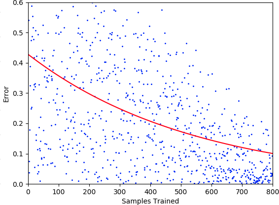
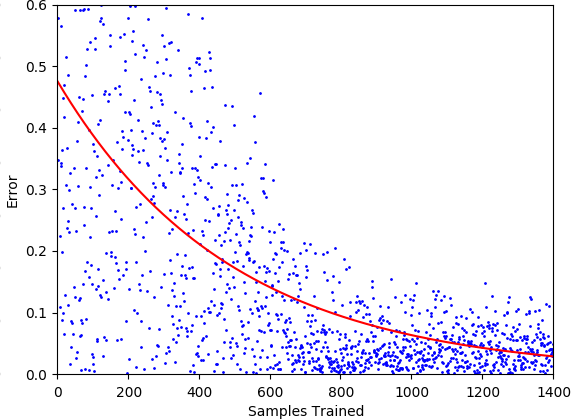
(a) Samples: 800, correlation coefficient: -0.54

(b) Samples: 1400, correlation coefficient: -0.65

Figure 1: Training a fully connnected neural network

6 Summary

This paper discussed a new narrative that offers structure and generality in describing neural networks, showing how they can be represented as recursive data structures, and their operations of forward and back propagation as recursion schemes. We demonstrated modularity in three particular ways: a delineation between the structure and semantics of a neural network, and compositionality in both neural network training and the types of layers in a network. Although only fully connected networks have been considered, we believe the ideas shown are transferrable to network types with more complex, sequential structure across multiple directions, and we have explored this externally with convolutional (§ 0.B.1) and recurrent (§ 0.B.2) networks in particular.

There are a number of interesting directions that are beyond the scope of this paper. One of these is performance, in particular, establishing to what extent we trade off computational efficiency in order to achieve generality in our approach. It is hoped that some of this can be offset by the performance gains of “fusion properties” [22] which the setting of structured recursion may give rise to; further insight would be needed as to the necessary circumstance for our implementation to exploit this. A second direction is to explore the many useful universal properties that recursion schemes enjoy, such as having unique solutions and being well-formed [13]; these may offer a means for equationally reasoning about the construction and evaluation of neural networks.

6.1 Related work

It has been long established that it is typically difficult to state and prove laws for arbitrary, explicitly recursive functions, and that structured recursion [11, 19, 20] can instead provide a setting where properties of termination and equational reasoning can be readily applied to programs [13]. Neural networks are not typically implemented using recursion, and are instead widely represented as directed graphs of computation calls [7]; the story between neural networks and recursion schemes hence has limited existing work. A particularly relevant discussion is presented by Olah [14] who corresponds the representation of neural networks to type theory in functional programming. This makes a number of useful intuitions, such as networks as chains of composed functions, and tree nets as catamorphisms and anamorphisms.

Neural networks have seen previous exploration in Haskell. Campbell [2] uses dependent types to implement recurrent neural networks, enabling type-safe composition of network layers of different shapes; here, networks are represented as heterogeneous lists of layers, and forward and back propagation over layer types as standard type class methods.

There is also work in the functional programming community on structured approaches towards graph types. Erwig [5] takes a compositional view of graph, and defines graph algorithms in terms of folds that can facilitate program transformations and optimizations via fusion properties. Oliveira and Cook [15] use parametric higher-order abstract syntax (PHOAS), and develop a language for representing structured graphs generically using fix points; operations on these graphs are then implemented as generalized folds.

Lastly, a categorical approach to deep learning has also been explored by Elliot [4], in particular towards automatic differentiation which is central in computing gradients during back propagation. They realise an intersection between category theory and computing derivatives of functions, and present a generalisation of automatic differentiation by replacing derivative values with an arbitrary cartesian category.

Appendix 0.A Elaborated code

0.A.1 Forward propagation

Below gives the full implementation of alg${}_{\scriptsize\textsf{fwd}}$ in § 3.1 for forward propagation.

⬇

type Values = [Double]

alg${}_{\scriptsize\textsf{fwd}}$ :: Layer [Values] $\rightarrow{}$ [Values]

alg${}_{\scriptsize\textsf{fwd}}$ (DenseLayer $w_{l}$ $b_{\,l}$ ($a_{l-1}\,$:$\,as$))

= ($a_{l}$ : $a_{l-1}\,$:$\,as$)

where $a_{l}$ = $\sigma(w_{l}*a_{l-1}+b_{l})$

– vector addition

$\oplus_{\tiny\textsf{v}}$ :: [Double] $\rightarrow{}$ [Double] $\rightarrow{}$ [Double]

xs $\oplus_{\tiny\textsf{v}}$ ys = zipWith (+) xs ys

– matrix-vector multiplication

$\otimes_{\tiny\textsf{mv}}$ :: [[Double]] $\rightarrow{}$ [Double] $\rightarrow{}$ [Double]

xss $\otimes_{\tiny\textsf{mv}}$ ys = map (sum $\circ$   zipWith (*) ys) yss

– sigmoid function

$\sigma$ :: [Double] $\rightarrow{}$ [Double]

$\sigma$ = map ($\lambda x$ $\rightarrow{}$ $1/(1+e^{-x})$)

0.A.2 Back propagation

Below gives the full implementation of backward, used during back propagation.

⬇

backward :: Weights $\rightarrow{}$ Biases $\rightarrow{}$ BackProp $\rightarrow{}$ (Deltas, Weights, Biases)

backward $w_{l}$ $b_{l}$ (BackProp $(a_{l}:a_{l-1}:as)\;w_{l+1}\;\delta_{l+1}$ desiredOutput) =

let $\delta_{l}$ = case $\delta_{l+1}$ of

[ ] $\rightarrow{}$ ($a_{l}\,\ominus_{\tiny\textsf{v}}$ desiredOutput) $\,\,\otimes_{\tiny\textsf{v}}\;\sigma^{\prime}(a_{l-1})\;$  – compute $\delta_{l}$ for final layer

$\underline{\;\;}$ $\rightarrow{}$ ((transpose $w_{l+1})\;\otimes_{\tiny\textsf{mv}}\;\delta_{l+1})\,\otimes_{\tiny\textsf{v}}\,\,\sigma^{\prime}(a_{l-1})$ – compute $\delta_{l}$ for any other layer

$w_{l}^{new}$ = $w_{l}\ominus_{\tiny\textsf{m}}(a_{l-1}\circledcirc\delta_{l})$

$b_{l}^{new}$   = $b_{l}\ominus_{\tiny\textsf{v}}\delta_{l}$

in ($\delta_{l}$, $w^{new}_{l}$, $b^{new}_{l}$)

– vector multiplication

$\otimes_{\tiny\textsf{v}}$ :: [Double] $\rightarrow{}$ [Double] $\rightarrow{}$ [Double]

xs $\otimes_{\tiny\textsf{v}}$ ys = zipWith (*) xs ys

– vector subtraction

$\ominus_{\tiny\textsf{v}}$ :: [Double] $\rightarrow{}$ [Double] $\rightarrow{}$ [Double]

xs $\ominus_{\tiny\textsf{v}}$ ys = zipWith (-) xs ys

– matrix subtraction

$\ominus_{\tiny\textsf{m}}$ :: [[Double]] $\rightarrow{}$ [[Double]] $\rightarrow{}$ [[Double]]

xss $\ominus_{\tiny\textsf{m}}$ yss = zipWith ($\ominus_{\tiny\textsf{v}}$) xs ys

– outer product

$\circledcirc$ :: [Double] $\rightarrow{}$ [Double] $\rightarrow{}$ [[Double]]

xs $\circledcirc$ ys = map ($\lambda$x $\rightarrow{}$ map (x *) ys) xs

– inverse then differential sigmoid function

$\sigma^{\prime}$ :: [Double] $\rightarrow{}$ [Double]

$\sigma^{\prime}$ = map ($\lambda$x $\rightarrow{}$ let y = log(x/(1 - x)) in y * (1 - y))

Appendix 0.B Training convolutional and recurrent networks

0.B.1 Training a convolutional neural network

Convolutional neural networks are used primarily to classify images. To demonstrate the ability of a convolutional network implementation to learn, we choose to classify matrix values as corresponding to either an image displaying the symbol ‘X’ or an image displaying the symbol ‘O’.

A diagram of the neural network used can be seen in Figure 2 where dimensions are given in the form (width $\times$ height $\times$ depth) $\times$ number of filters. An input image of dimensions ($7\times 7\times 1$) is provided to the network, resulting in an output vector of length two where each value corresponds to the probability of the image being classified as either an ‘X’ or an ‘O’ symbol.

Figure 2: Convolutional network

The network above is constructed by convNetwork, whose type ConvNetwork is the coproduct of five possible layer types found in a convolutional network:

⬇

type ConvNetwork = (InputLayer :+: DenseLayer :+: ConvLayer :+: PoolLayer :+: ReLuLayer)

convNetwork :: Free ConvNetwork a

convNetwork = do

denselayer (randMat2D 2 2)    (zeroMat1D 2)

convlayer (randMat4D 2 2 1 2) (zeroMat2D 2 1)

convlayer (randMat4D 2 2 4 1) (zeroMat2D 1 1)

poollayer 2 1

convlayer (randMat4D 3 3 1 4) (zeroMat2D 1 1)

inputlayer

In Figure 3, we see the change in error as the amount of trained samples increases, using sample sizes of 300 and 600. The negative curvature demonstrates the convolutional neural network is successful in learning to classify the provided images. Two distinct streams of blue dots can also be observed in each graph, which represent the different paths of error induced by both of the sample types. The negative correlation coefficient is stronger in magnitude when using a sample size of 600, showing a better rate of convergence for the larger data set.

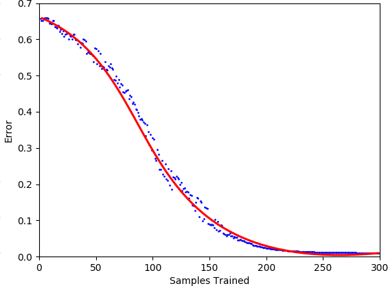
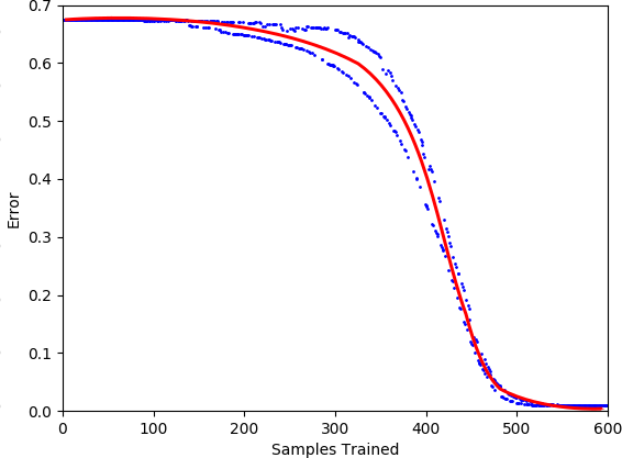
(a) Samples: 300, correlation coefficient: -0.747

(b) Samples: 600, correlation coefficient: -0.876

Figure 3: Training a convolutional neural network

0.B.2 Training a recurrent neural network

Recurrent networks are primarily used for classifying sequential time-series data in tasks such as text prediction, hand writing recognition or speech recognition. To demonstrate the functionality of our recurrent network implementation, we use DNA strands as data — these can be represented using the four characters a, t, c, and g. Given a strand of five DNA characters, our network will attempt to learn the next character in the sequence.

A diagram of the recurrent network used is shown in Figure 4, consisting of two layers of five cells. We omit its corresponding implementation, but note that training over this network structure is represented by a catamorphism over layers where the algebra is a catamorphism over the cells of the layer.

Figure 4: Recurrent network

In Figure 5, we see the change in error as the amount of trained samples increases, using sample sizes of 300 and 600. The negative curvature shown is less noticeable than the tests performed on previous networks, but still present. In contrast to the previous results, the correlation coefficient for the larger sample size of 600 is lower in magnitude than for the sample size of 300, perhaps showing convergence early on; achieving more conclusive results would require a more informed approach to the architecture and design of recurrent networks.

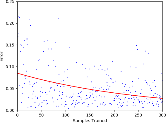
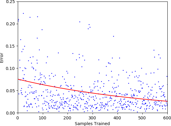
(a) Samples: 300, correlation coefficient: -0.314

(b) Samples: 600, correlation coefficient: -0.254

Figure 5: Training a recurrent neural network

References

- [1] Bebis, G., Georgiopoulos, M.: Feed-forward neural networks. IEEE Potentials 13(4), 27–31 (1994)
- [2] Campbell, H.: Grenade. https://github.com/HuwCampbell/grenade (2017)
- [3] Chollet, F., et al.: Keras (2015), https://github.com/fchollet/keras
- [4] Elliott, C.: The simple essence of automatic differentiation. Proceedings of the ACM on Programming Languages 2(ICFP), 1–29 (2018)
- [5] Erwig, M.: Functional programming with graphs. ACM SIGPLAN Notices 32(8), 52–65 (1997)
- [6] Gibbons, J.: Streaming representation-changers. In: International Conference on Mathematics of Program Construction. pp. 142–168. Springer (2004)
- [7] Guresen, E., Kayakutlu, G.: Definition of artificial neural networks with comparison to other networks. Procedia Computer Science 3, 426–433 (2011)
- [8] Hinton, G.E.: Deep belief networks. Scholarpedia 4(5), 5947 (2009)
- [9] Hinze, R., Wu, N., Gibbons, J.: Unifying structured recursion schemes. ACM SIGPLAN Notices 48(9), 209–220 (2013)
- [10] Khashman, A.: Application of an emotional neural network to facial recognition. Neural Computing and Applications 18(4), 309–320 (2009)
- [11] Malcolm, G.: Data structures and program transformation. Science of computer programming 14(2-3), 255–279 (1990)
- [12] Medsker, L.R., Jain, L.: Recurrent neural networks. Design and Applications 5, 64–67 (2001)
- [13] Meijer, E., Fokkinga, M., Paterson, R.: Functional programming with bananas, lenses, envelopes and barbed wire. In: Conference on functional programming languages and computer architecture. pp. 124–144. Springer (1991)
- [14] Olah, C.: Neural networks, types, and functional programming. https://colah.github.io/posts/2015-09-NN-Types-FP/
- [15] Oliveira, B.C., Cook, W.R.: Functional programming with structured graphs. In: Proceedings of the 17th ACM SIGPLAN international conference on Functional programming. pp. 77–88 (2012)
- [16] Paszke, A., Gross, S., Massa, F., Lerer, A.: Pytorch: An imperative style, high-performance deep learning library. In: Wallach, H., Larochelle, H., Beygelzimer, A., d'Alché-Buc, F., Fox, E., Garnett, R. (eds.) Advances in Neural Information Processing Systems 32, pp. 8024–8035. Curran Associates, Inc. (2019)
- [17] Svozil, D., Kvasnicka, V., Pospichal, J.: Introduction to multi-layer feed-forward neural networks. Chemometrics and intelligent laboratory systems 39(1), 43–62 (1997)
- [18] Swierstra, W.: Data types à la carte. Journal of functional programming 18(4), 423–436 (2008)
- [19] Uustalu, T., Vene, V.: Primitive (co) recursion and course-of-value (co) iteration, categorically. Informatica 10(1), 5–26 (1999)
- [20] Vene, V., Uustalu, T.: Functional programming with apomorphisms (corecursion). In: Proceedings of the Estonian Academy of Sciences: Physics, Mathematics. vol. 47, pp. 147–161 (1998)
- [21] Wang, W., Huang, Y., Wang, Y., Wang, L.: Generalized autoencoder: A neural network framework for dimensionality reduction. In: Proceedings of the IEEE conference on computer vision and pattern recognition workshops. pp. 490–497 (2014)
- [22] Wu, N., Schrijvers, T.: Fusion for free. In: International Conference on Mathematics of Program Construction. pp. 302–322. Springer (2015)
- [23] Wu, N., Schrijvers, T., Hinze, R.: Effect handlers in scope. In: Proceedings of the 2014 ACM SIGPLAN Symposium on Haskell. pp. 1–12 (2014)
- [24] Yamashita, R., Nishio, M., Do, R.K.G., Togashi, K.: Convolutional neural networks: an overview and application in radiology. Insights into imaging 9(4), 611–629 (2018)
- [25] Yih, W.t., He, X., Meek, C.: Semantic parsing for single-relation question answering. In: Proceedings of the 52nd Annual Meeting of the Association for Computational Linguistics (Volume 2: Short Papers). pp. 643–648 (2014)