Pixelated Reconstruction of Gravitational Lenses using Recurrent Inference Machines

Abstract

Modeling strong gravitational lenses in order to quantify the distortions in the images of background sources and to reconstruct the mass density in the foreground lenses has traditionally been a difficult computational challenge. As the quality of gravitational lens images increases, the task of fully exploiting the information they contain becomes computationally and algorithmically more difficult. In this work, we use a neural network based on the Recurrent Inference Machine (RIM) to simultaneously reconstruct an undistorted image of the background source and the lens mass density distribution as pixelated maps. The method we present iteratively reconstructs the model parameters (the source and density map pixels) by learning the process of optimization of their likelihood given the data using the physical model (a ray-tracing simulation), regularized by a prior implicitly learned by the neural network through its training data. When compared to more traditional parametric models, the proposed method is significantly more expressive and can reconstruct complex mass distributions, which we demonstrate by using realistic lensing galaxies taken from the cosmological hydrodynamic simulation IllustrisTNG.

1 Introduction

Strong gravitational lensing is a natural phenomenon through which multiple distorted images of luminous background objects, i.e. early-type star-forming galaxies, are formed by massive foreground objects along the line of sight (e.g., Vieira et al., 2013; Marrone et al., 2018; Rizzo et al., 2020; Sun et al., 2021). These distortions are tracers of the distribution of mass in foreground objects, independent of the electromagnetic behaviour of these overdensities. As such, this phenomenon offers a powerful probe of the distribution of dark matter and its properties outside of the Milky Way (e.g., Dalal & Kochanek, 2002; Treu & Koopmans, 2004; Hezaveh et al., 2016; Gilman et al., 2020, 2021).

Lens modeling is the process of inferring the parameters describing both the mass distribution in the foreground lens and the light emitted by the background source. This has traditionally been a time- and resource-consuming procedure. A common practice to model the mass of lensing galaxies is to assume that the density profiles follow simple parametric forms, e.g., a power law $\rho\propto r^{-\gamma^{\prime}}$. These profiles generally provide a good fit to low-resolution data and are easy to work with due to their small number of parameters (e.g., Koopmans et al., 2006; Barnabè et al., 2009; Auger et al., 2010). However, as high-resolution and high signal-to-noise ratio (SNR) images become available, lens analysis with simple models requires introducing additional parameters representing the complexities in the lensing galaxies and their immediate environments (e.g., Sluse et al., 2017; Wong et al., 2017; Birrer et al., 2019; Rusu et al., 2020, 2017; Li et al., 2021). This approach becomes intractable as the quality of images increases. For example, no simple parametric model of the Hubble Space Telescope (HST) Wide Field Camera 3 (WFC3) images of the Cosmic Horseshoe (J1148+1930) — initially discovered by Belokurov et al. (2007) — has been able to model the fine features of the extended arc (e.g., Bellagamba et al., 2016; Cheng et al., 2019; Schuldt et al., 2019).

In this work, we develop a method for pixelated strong gravitational lensing mass and source reconstruction, allowing it to reconstruct complex distributions. Our method is based on the Recurrent Inference Machine (RIM, Putzky & Welling, 2017), which proposes to learn an iterative inference algorithm, moving away from hand-chosen inference algorithms and hand-crafted priors. In this framework, the prior is implicit in the dataset used to train the neural network. We also present a new architecture based on the original RIM to allow the inference of pixelated maps for this highly non-linear and under-constrained problem.

2 Methods

2.1 Data

The background source brightness distributions are taken from the Hubble Space Telescope (HST) COSMOS field (Koekemoer et al., 2007; Scoville et al., 2007), acquired in the F814W filter. A dataset of mag limited ($\mathrm{F814W}<23.5$) deblended galaxy postage stamps (Leauthaud et al., 2007) was compiled as part of the GREAT3 challenge (Mandelbaum et al., 2014). The data is publicly available (Mandelbaum et al., 2012), and the preprocessing is done through the open-source software GALSIM (Rowe et al., 2015). The final set has $13\,321$ galaxy images cropped to $128^{2}$ pixels and with a flux greater than $50\,\,\mathrm{photons}\,\,\mathrm{cm}^{-2}\,\mathrm{s}^{-1}$. We split this set into a training set (90%) and a test set (10%) before data augmentation and denoising with an autoencoder (Vincent et al., 2008).

The projected surface density maps (convergence) of lensing galaxies were made using the redshift $z=0$ snapshot of the IllustrisTNG-100 simulation (Nelson et al., 2019) in order to produce physically realistic realizations of dark matter and baryonic matter halos. We selected 1604 profiles, split into a training set ($90\%$) and a test set ($10\%$), with the criteria that they have a total dark matter mass of at least $9\times 10^{11}M_{\odot}$. We then collected all dark matter, gas, stars, and black hole particles from the profiles. We then compute smoothed projected surface density maps with an adaptive Gaussian kernel following the prescriptions from Aubert et al. (2007) and Rau et al. (2013). The final training set is composed of 3 different projections ($xy$, $xz$ and $yz$) of each profiles, rendered on a pixelated grid with a resolution of $0.55\,\mathrm{kpc}/h$ and $128^{2}$ pixels. Several data augmentation rounds, including rescaling each convergence maps randomly to produce a set with an Einstein radius uniformly distributed ${\theta_{E}\sim\mathcal{U}(0.5^{\prime\prime},2.5^{\prime\prime})}$, were used to increase the number of profiles to $50\,000$ for training a VAE and the RIM.

2.2 Data Augmentation with VAEs

When working with limited data, data augmentation is crucial to ensure that the trained model is robust against perturbations — like rotations of images — which are not implicitly included as symmetries in the architecture of the model. We trained a variational auto-encoder (VAE, Kingma & Welling, 2013) for data augmentation of the source maps and another VAE for the convergence maps.

Direct optimization of the ELBO loss for VAEs can prove difficult because the reconstruction term could be relatively weak compared to the Kullback Leibler (KL) divergence term (Kingma & Welling, 2019). To alleviate this issue, we follow the work of Bowman et al. (2015) and Kaae Sønderby et al. (2016) in setting a warm-up schedule for the KL term in the ELBO loss, starting from $\beta=0.1$ up to $\beta_{\mathrm{max}}$. Following the work of Lanusse et al. (2021), we also introduce an $\ell_{2}$ penalty between the input and output of the bottleneck fully-connected layers to encourage an identity map between them. This regularisation term is slowly removed during training.

Figure 1: Example of a simulated lensed image in the test set that exhibits a large deflection in its eastern arc which indicates the presence of a massive object — in this case a dark matter subhalo. The fine-tuning procedure is able to recover this subhalo because of its strong signal in the lensed image and reduces the residuals to noise level.

2.3 Raytracing

Simulations of lensed images are produced using a ray-tracing code, which maps the brightness distribution of background sources to the observed coordinates. The foreground pixel coordinates $\bm{\theta}_{i}$ and the source pixel coordinates $\bm{\beta}_{i}$ are related by the lens equation

$$\bm{\beta}_{i}=\bm{\theta}_{i}-\bm{\alpha}(\bm{\theta}_{i}),$$ (1)

where $\bm{\alpha}$ is the deflection angle. The deflection angle is calculated from the projected surface density field $\kappa$ (also commonly refered to as the convergence) by the integral

$$\bm{\alpha}(\bm{\theta}_{i})=\frac{1}{\pi}\int_{\mathbb{R}^{2}}\kappa(\bm{\theta}^{\prime})\frac{\bm{\theta}_{i}-\bm{\theta}^{\prime}}{\lVert\bm{\theta}_{i}-\bm{\theta}^{\prime}\rVert^{2}}d^{2}\bm{\theta}^{\prime}$$ (2)

The intensity of a pixel in a simulated lensed image is obtained by bilinear interpolation of the source brightness distribution at the coordinate $\bm{\beta}_{i}$. The integral in equation (2) is computed in near-linear time using Fast Fourier Transforms (FFT).

A blurring operator — i.e., a convolution by a point spread function — is then applied to the lensed image to replicate the response of an imaging system. This operator is implemented as a GPU-accelerated matrix operation since the blurring kernels used in this paper have a significant proportion of their energy distribution encircled inside a small pixel radius.

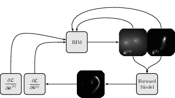
Figure 2: Rolled computational graph of the RIM.

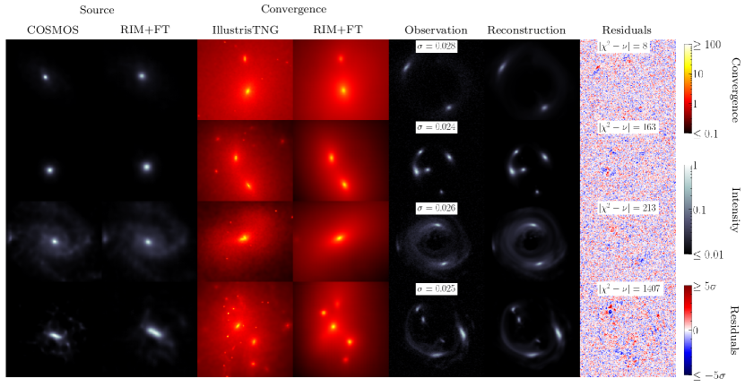
Figure 3: Samples of the fine-tuned RIM (RIM+FT) reconstructions from the test set. We report the residuals of the reconstruction, as well as the difference between the $\chi^{2}$ and the number of degrees of freedom $\nu=16384$.

2.4 Recurrent Inference Machine

The RIM (Putzky & Welling, 2017) is a form of learned gradient-based inference intended to solve inverse problems of the form

$$\mathbf{y}=f(\mathbf{x})+\mathcal{N}\,,$$ (3)

where $\mathbf{y}$ is a vector of noisy lensed images, $f$ is a function encoding the physical model, $\mathbf{x}$ is a vector of parameters of interest, and $\mathcal{N}$ is a vector of additive noise. This framework has been applied in the context of linear inverse problems, where the function $f$ can be represented in a matrix form, in particular in the cases of under-constrained problems for which the prior on the parameters $\mathbf{x}$, $p(\mathbf{x})$, is either intractable or hard to compute (Morningstar et al., 2018, 2019; Lønning et al., 2019). The use of the RIM to solve non-linear inverse problems was first investigated in (Modi et al., 2021). In our case, the inverse problem mapping function $F$ is non-linear w.r.t. the convergence parameters which is a consequence of the non-linearity of equation (1).

The governing equation for the RIM is a recurrent relation that takes the general form

$$\mathbf{\hat{x}}^{(t+1)}=\mathbf{\hat{x}}^{(t)}+g_{\varphi}\big{(}\mathbf{\hat{x}}^{(t)},\,\mathbf{y},\,\gradient_{\mathbf{\hat{x}^{(t)}}}\log p(\mathbf{y}\mid\mathbf{x}^{(t)})\big{)}\,,$$ (4)

where $p(\mathbf{y}\mid\mathbf{x})$ is an isotropic gaussian likelihood function, characterized by the noise standard deviation $\sigma$. By minimizing the weighted mean squared loss

$$\mathcal{L}_{\varphi}(\mathbf{x},\mathbf{y})=\frac{1}{T}\sum_{t=1}^{T}\sum_{i=1}^{M}\mathbf{w}_{i}(\mathbf{\hat{x}}^{(t)}_{i}-\mathbf{x}_{i})^{2}\,,$$ (5)

the RIM learns to optimize the parameters $\mathbf{x}$ given a likelihood function. Unlike previous work (Andrychowicz et al., 2016; Putzky & Welling, 2017; Morningstar et al., 2018, 2019; Lønning et al., 2019), the data vector $\mathbf{y}$ — or observation — is fed to the neural network in order to learn the initialization of the parameters, $\mathbf{\hat{x}}^{(0)}=g_{\varphi}(0,\mathbf{y},0)$, as well as their optimization. We found in practice that this significantly improves the performance of the model for our problem and it avoids situations where the model would get stuck in local minima at test time due to poor initialization.

The RIM used in this work is designed based on a U-net architecture (Ronneberger et al., 2015). The most important aspect of our implementation is the use of Gated Recurrent Units (Cho et al., 2014) placed in each skip connection which guides the reconstruction independently at different levels of resolution. The gradient of the likelihood is computed using automatic differentiation. Following Modi et al. (2021), we preprocess the gradients using the Adam algorithm (Kingma & Welling, 2013).

2.5 Fine-tuning

Once the RIM is trained, we can treat the RIM optimization procedure as a baseline estimator of the parameters $\mathbf{x}$ given a noisy observation $\mathbf{y}$. We now concern ourselves with a strategy to improve this estimator. This is important for observations with high SNR, for which the estimator must be extremely accurate to model all the fine features present in the arcs. The fine-tuning objective is to minimize directly the likelihood over each time steps of the RIM:

$$\hat{\varphi}_{\mathrm{MAP}}=\underset{\varphi}{\mathrm{argmax}}\,\,\frac{1}{T}\sum_{t=1}^{T}\log p(\mathbf{y}\mid\mathbf{\hat{x}}^{(t)})+\log p(\varphi)\,.$$ (6)

This objective function makes no use of labels, meaning that only an observation $\mathbf{y}$ is required to fine-tune the RIM. This allows us to use this objective at test time, at which point the RIM is trained to reconstruct this specific observation.

We use elastic weight consolidation (EWC, Kirkpatrick et al., 2016) as prior over the model parameters. To compute the Fisher matrix in EWC, it is necessary to sample from a distribution of lensing systems that are conditioned on the observation. This is accomplished by sampling the latent space of both the source VAE and the convergence VAE near the latent code of the baseline prediction of the RIM. More details regarding this procedure are given in appendix E.

3 Results and Discussion

Figure 3 presents a few examples of the reconstructions obtained using the approach presented above. An emphasis is put on complex convergence profiles with multiple main deflectors or substructures. Modeling such convergence maps with traditional maximum-likelihood methods using analytical profiles would require significant user input and considerable computational resources due to large parameter degeneracies. The mock observations as well as the reconstructed lensed images are also shown, alongside the residuals of the reconstructions and the $\chi^{2}$ statistic. The first 3 reconstructions have statistically significant residuals, with no pixels exceeding the $5\sigma$ threshold. The last reconstruction, which is arguably the most complex to perform, has a few pixels reaching $5\sigma$.

In addition to a visual inspection of the reconstructed sources and convergences, we compute the coherence spectrum to quantitatively assess the quality the reconstructions

$$\gamma(k)=\frac{P_{12}(k)}{\sqrt{P_{11}(k)P_{22}(k)}}\,,$$ (7)

where $P_{ij}(k)$ is the cross power spectrum of images $i$ and $j$ at the wavenumber $k$. Figure 4 shows the mean value and the $68\%$ inclusion interval of those spectra for the convergence and source maps in a test set of 3000 examples. The fine-tuning procedure, shown in red, is able to improve significantly the coherence of the baseline background source, shown in black, at all scales. The coherence spectrum of the convergence remains unchanged by the fine-tuning procedure. Still, we note that many examples in the dataset showcase significant improvement which we illustrate in Figure 1.

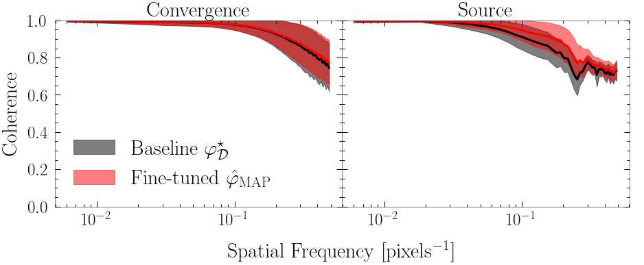
Figure 4: Statistics of the coherence spectrum from a test set. The solid line is the average coherence. The transparent region is the $68\%$ confidence interval.

The results obtained here demonstrate the effectiveness of machine learning methods for inferring pixelated maps of the distribution of mass in lensing galaxies. Since this is a heavily under-constrained problem, stringent priors are needed to avoid overfitting the data, a task that has traditionally been difficult to accomplish (e.g., Saha & Williams, 1997). The model proposed here can implicitly learn these priors from a set of training data.

The flexible and expressive form of the reconstructions means that, in principle, any lensing system (e.g., a single simple galaxy, or a group of complex galaxies) could be analyzed by this model, without any need for pre-determining the model parameterization. This is of high value given the diversity of observed lensing systems, and their relevance for constraining astrophysical and cosmological parameters.

Software and data

The source code, as well as the various scripts and parameters used to produce the model and results is available as open-source software under the package Censai. The model parameters, as well as the convergence maps and the background sources used to train these models, the test set examples and the reconstructions results are available as open-source datasets hosted by Zenodo. This research made use of Tensorflow (Abadi et al., 2015), Tensorflow-Probability (Dillon et al., 2017), Numpy (Harris et al., 2020), Scipy (Virtanen et al., 2020), Matplotlib (Hunter, 2007), scikit-image (Van der Walt et al., 2014), IPython (Pérez & Granger, 2007), Pandas (Wes McKinney, 2010; pandas development team, 2020), Scikit-learn (Pedregosa et al., 2011), Astropy (Astropy Collaboration et al., 2013, 2018) and GalSim (Rowe et al., 2015).

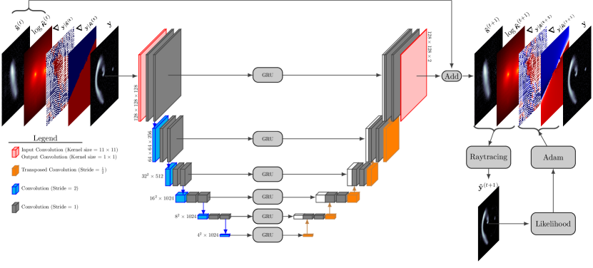
Figure 5: A single time step of the unrolled computation graph of the RIM. GRU units are placed in the skip connections to guide the reconstruction of the source and convergence. A diagram of the steps to compute the likelihood gradients is shown in the bottom right of the figure, including the Adam processing step. We used the shorthand notation $\gradient_{\mathbf{y}\mid\mathbf{x}}\equiv\gradient_{\mathbf{x}}\log p(\mathbf{y}\mid\mathbf{x})$, $\mathbf{s}$ to mean the source map and $\log\bm{\kappa}$ to mean the $\log_{10}$ of the convergence map.

Appendix A Training dataset

$400\,000$ observations are simulated from random pairs of COSMOS sources and IllustrisTNG convergence training splits in order to train the RIM. An additional $200\,000$ observations are created from pairs of COSMOS source and pixelated singular isothermal elliptical (SIE) convergence maps. $1\,600\,000$ simulated observations are also generated from the VAE background sources and convergence maps as part of the training set. Validation checks are applied to each examples in order to avoid configurations like a single image of the background source or an Einstein ring cropped by the field of view.

Table 1: SIE parameters.

Parameter	Distribution
Radial shift (”)	$\mathcal{U}(0,0.1)$
Azimutal shift	$\mathcal{U}(0,2\pi)$
Orientation	$\mathcal{U}(0,\pi)$
$\theta_{E}$ (”)	$\mathcal{U}(0.5,2.5)$
Ellipticity	$\mathcal{U}(0,0.6)$

Appendix B Data augmentation with VAE

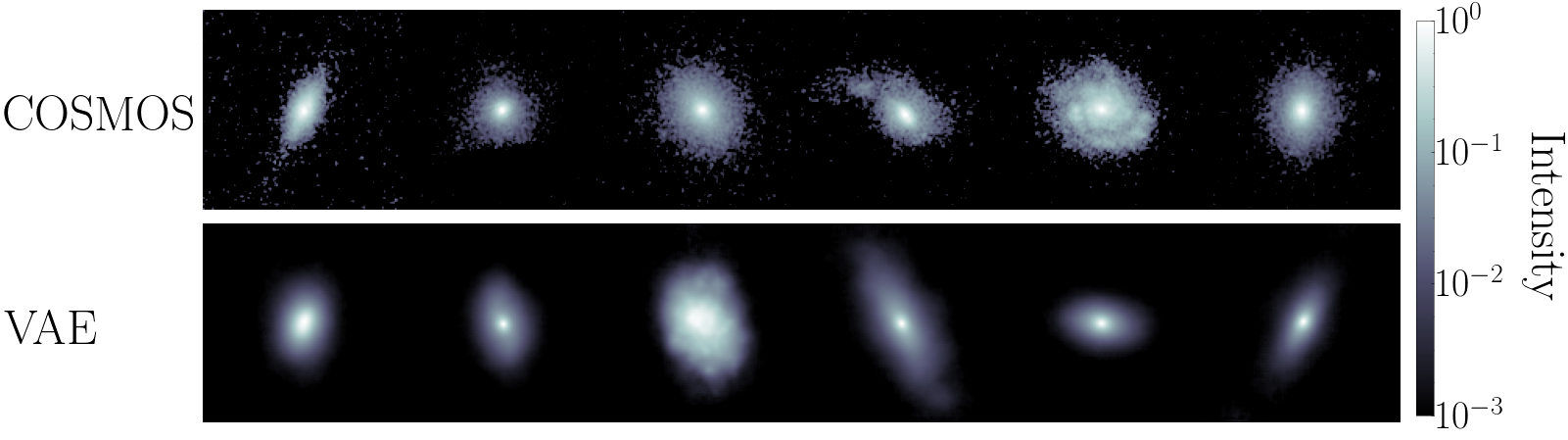
(a) Examples of COSMOS galaxy images (top row) and VAE generated samples (bottom row).

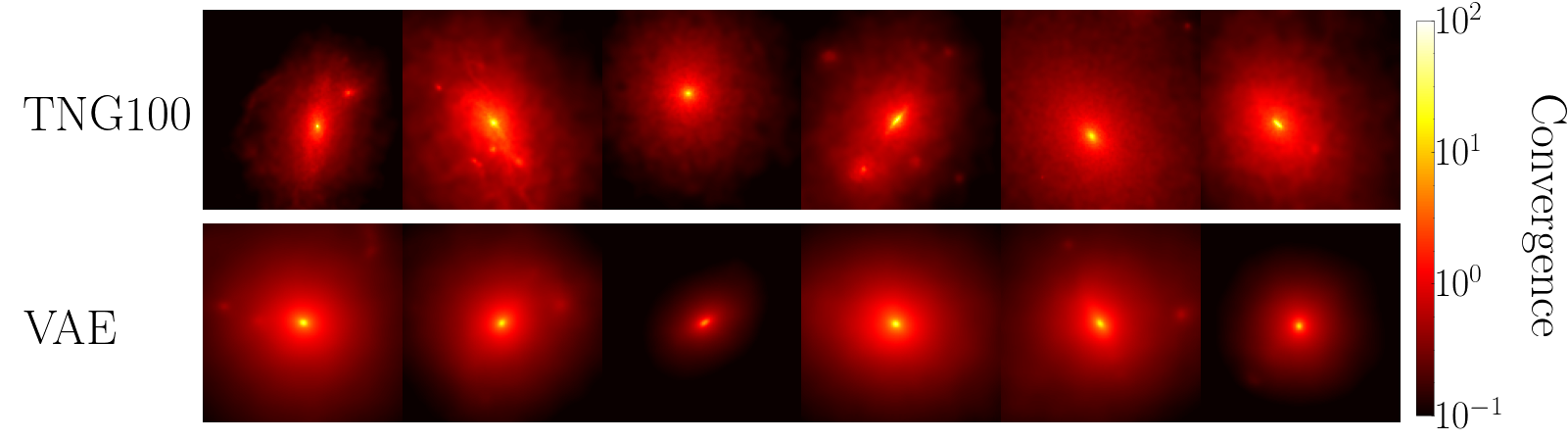
(b) Examples of smoothed Illustris TNG100 convergence map (top row) and VAE generated samples (bottom row).

Figure 6: Labels for the training set.

Appendix C VAE Architecture and optimisation

For the following architectures, we employ the notion of level to mean layers in the encoder and the decoder with the same spatial resolution. In each level, we place a block of convolutional layers before downsampling (encoder) or after upsampling (decoder). These operations are done with strided convolutions like in the U-net architecture of the RIM.

Table 2: Hyperparameters for the background source VAE.

Parameter	Value
Input preprocessing	1
Architecture
Levels (encoder and decoder)	3
Convolutional layer per level	2
Latent space dimension	32
Hidden Activations	Leaky ReLU
Output Activation	Sigmoid
Filters	16, 32, 64
Number of parameters	$3\,567\,361$
Optimization
Optimizer	Adam
Initial learning rate	$10^{-4}$
Learning rate schedule	Exponential Decay
Decay rate	0.5
Decay steps	$30\,000$
Number of steps	$500\,000$
$\beta_{\mathrm{max}}$	0.1
Batch size	20

Table 3: Hyperparameters for the convergence VAE.

Parameter	Value
Input preprocessing	$\log_{10}$
Architecture
Levels (encoder and decoder)	4
Convolutional layer per level	1
Latent space dimension	16
Hidden Activations	Leaky ReLU
Output Activation	1
Filters	16, 32, 64, 128
Number of parameters	$1\,980\,033$
Optimization
Optimizer	Adam
Initial learning rate	$10^{-4}$
Learning rate schedule	Exponential Decay
Decay rate	0.7
Decay steps	$20\,000$
Number of steps	$155\,000$
$\beta_{\mathrm{max}}$	0.2
Batch size	32

Appendix D RIM architecture and optimisation

The notion of link function $\Psi:\Xi\rightarrow\mathcal{X}$, introduced by Putzky & Welling (2017), is an invertible transformation between the network prediction space $\bm{\xi}\in\Xi$ and the forward modelling space $\mathbf{x}\in\mathcal{X}$. This is a different notion from preprocessing, discussed in section 2.1, because this transformation is applied inside the recurrent relation 4 as opposed to before training. In the case where the forward model has some restricted support or it is found that some transformation helps the training, then the link function chosen must be implemented as part of the network architecture as shown in the unrolled computational graph in Figure 7. Also, the loss $\mathcal{L}_{\varphi}$ must be computed in the $\Xi$ space in order to avoid gradient vanishing problems when $\Psi$ is a non-linear mapping, which happens if the non-linear link function is applied in an operation recorded for backpropagation through time (BPTT).

For the convergence, we use an exponential link function with base $10$: $\bm{\hat{\kappa}}=\Psi(\bm{\xi})=10^{\bm{\xi}}$. This $\Psi$ encodes the non-negativity of the convergence. Furthermore, it is a power transformation that leaves the linked pixel values $\bm{\xi}_{i}$ normally distributed, thus improving the learning through the non-linearities in the neural network. The pixel weights $\mathbf{w}_{i}$ in the loss function (5) are chosen to encode the fact that the pixel with critical mass density ($\bm{\kappa}_{i}>1$) have a stronger effect on the lensing configuration than other pixels. We find in practice that the weights

$$\mathbf{w}_{i}=\frac{\sqrt{\bm{\kappa}_{i}}}{\sum_{i}\bm{\kappa}_{i}},$$ (8)

encode this knowledge in the loss function and improved both the empirical risk and the goodness of fit of the baseline model on early test runs.

For the source, we found that we do not need a link function — its performance is generally better compared to other link function we tried like sigmoid and power transforms — and we found that the pixel weights can be taken to be uniform, i.e. $\mathbf{w}_{i}=\frac{1}{M}$.

In the first optimisation stage, we trained 24 different architectures from a small set of valid hyperparameters previously identified for approximately 4 days (wall time using a single Nvidia A100 gpu). Following this first stage, 4 architectures were deemed efficient enough to be trained for an additional 6 days.

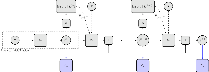
Figure 7: Unrolled computational graph of the RIM. Operations along solid arrows are being recorded for BPTT, while operations along dashed arrows are not. The blue arrows are only used for optimisation during training. During fine-tuning or testing, the loss is computed only as an oracle metric to validate that our methods can recover the ground truth.

Table 4: Hyperparameters for the RIM.

Parameter	Value
Source link function	1
$\kappa$ link function	$10^{\bm{\xi}}$
Architecture	Figure 5
Recurrent steps ($T$)	8
Number of parameters	$348\,546\,818$
First Stage Optimisation
Optimizer	Adamax
Initial learning rate	$10^{-4}$
Learning rate schedule	Exponential Decay
Decay rate	0.95
Decay steps	$100\,000$
Number of steps	$610\,000$
Batch size	1
Second Stage Optimisation
Optimizer	Adamax
Initial learning rate	$6\times 10^{-5}$
Learning rate schedule	Exponential Decay
Decay rate	0.9
Decay steps	$100\,000$
Number of steps	$870\,000$
Batch size	1

Appendix E Fine-Tuning

We follow the work of Kirkpatrick et al. (2016) to define a prior distribution over $\varphi$ that address the issue of catastrophic forgetting (McCloskey & Cohen, 1989; Ratcliff, 1990):

$$\log p(\varphi)\propto-\frac{\lambda}{2}\sum_{j}\mathrm{diag}(\mathcal{I}(\varphi_{\mathcal{D}}^{\star}))_{j}(\varphi_{j}-[\varphi^{\star}_{\mathcal{D}}]_{j})^{2},$$ (9)

where $\mathrm{diag}(\mathcal{I}(\varphi_{\mathcal{D}}^{\star}))$ is the diagonal of the Fisher information matrix encoding the amount of information that some set of gravitational lensing systems from the training set similar to the observed test task carries about the baseline RIM weights $\varphi_{\mathcal{D}}^{\star}$ — the parameters that minimize the empirical risk over the training dataset $\mathcal{D}$. The Lagrange multiplier $\lambda$ is tuning our estimated uncertainty about the neural network weights for the particular task at hand.

We can understand the need for a conditional sampling distribution by looking at the posterior of the RIM parameters. Suppose we are given a training set $\mathcal{D}$ and a test task $\mathcal{T}$ which are conditionally independent given $\varphi$ and have uniform priors, then the posterior of the RIM parameters $\mathcal{\varphi}$ can be rewritten using the Bayes rule as

$$p(\varphi\mid\mathcal{D},\,\mathcal{T})=\frac{p(\mathcal{T}\mid\varphi)p(\varphi\mid\mathcal{D})}{p(\mathcal{T}\mid\mathcal{D})}\,.$$ (10)

The sampling distribution in this expression appears as the conditional $p(\mathcal{T}\mid\mathcal{D})$, which can also be viewed as the set of examples from the training set similar to the test task by rewriting it as $p(\mathcal{T}\mid\mathcal{D})\propto p(\mathcal{D}\mid\mathcal{T})$. The EWC term is then derived by a Laplace approximation of the prior $p(\varphi\mid\mathcal{D})$ around $\varphi_{\mathcal{D}}^{\star}$, which we also take to be proportional to the training loss, the likelihood of each time steps and an $\ell_{2}$ loss

$$\log p\big{(}\varphi\mid(\mathbf{x},\mathbf{y})=\mathcal{D}\big{)}\propto-\mathcal{L}_{\varphi}(\mathbf{x},\mathbf{y})+\frac{1}{T}\sum_{t=1}^{T}\log p(\mathbf{y}\mid\mathbf{\hat{x}}^{(t)})-\frac{\ell_{2}}{2}\lVert\varphi\rVert^{2}_{2}\,.$$ (11)

Each reconstruction is performed by fine-tuning the baseline model on a test task composed of an observation vector, a PSF and a noise amplitude. In practice, fine-tuning the test set of $3\,000$ examples can be accomplished in parallel so as to be done in at most a few days by spreading the computation on $\sim 10$ Nvidia A100 GPUs (or 10 hours on $\sim 100$ GPUs). Each reconstruction uses at most 2000 steps, which turns out to be approximately $20$ minutes (wall-time) per reconstruction. Early stopping is applied when the $\chi^{2}$ reaches noise level ($\chi^{2}=\nu$).

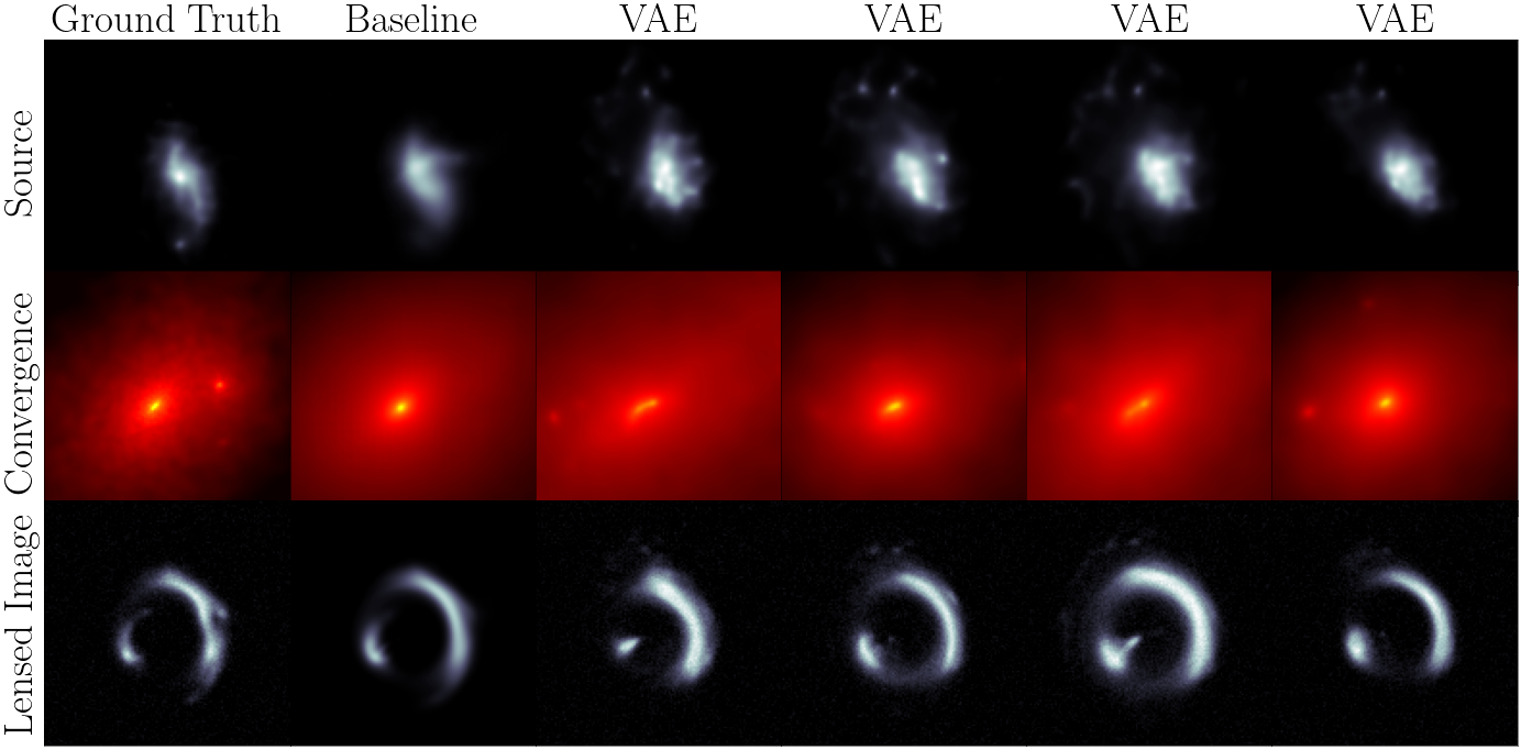
Figure 8: Examples similar to the test task shown in Figure 3. They are sampled from the latent space of the source VAE and convergence VAE near the RIM baseline latent code $\mathbf{\hat{z}}^{(T)}$ and used to estimate $\mathrm{diag}(\mathcal{I}(\varphi^{\star}_{\mathcal{D}}))$.

Table 5: Hyperparameters for fine-tuning the RIM.

Parameter	Value
Optimizer	RMSProp
Learning rate	$10^{-6}$
Maximum number of steps	$2\,000$
$\lambda$	$2\times 10^{5}$
$\ell_{2}$	0
Number of samples from VAE	200
Latent space distribution	$\mathcal{N}(\mathbf{\hat{z}}^{(T)},\sigma=0.3)$

Figure 9: 30 reconstructions taken at random from the test set of 3000 examples simulated from COSMOS and IllustrisTNG data at high SNR. The colorscale are the same as in Figure 3.

References

- Abadi et al. (2015) Abadi, M., Agarwal, A., Barham, P., Brevdo, E., Chen, Z., Citro, C., Corrado, G. S., Davis, A., Dean, J., Devin, M., Ghemawat, S., Goodfellow, I., Harp, A., Irving, G., Isard, M., Jia, Y., Jozefowicz, R., Kaiser, L., Kudlur, M., Levenberg, J., Mané, D., Monga, R., Moore, S., Murray, D., Olah, C., Schuster, M., Shlens, J., Steiner, B., Sutskever, I., Talwar, K., Tucker, P., Vanhoucke, V., Vasudevan, V., Viégas, F., Vinyals, O., Warden, P., Wattenberg, M., Wicke, M., Yu, Y., and Zheng, X. TensorFlow: Large-scale machine learning on heterogeneous systems, 2015. Software available from tensorflow.org.
- Andrychowicz et al. (2016) Andrychowicz, M., Denil, M., Gomez, S., Hoffman, M. W., Pfau, D., Schaul, T., Shillingford, B., and de Freitas, N. Learning to learn by gradient descent by gradient descent. arXiv e-prints, art. arXiv:1606.04474, June 2016.
- Astropy Collaboration et al. (2013) Astropy Collaboration, Robitaille, T. P., Tollerud, E. J., Greenfield, P., Droettboom, M., Bray, E., Aldcroft, T., Davis, M., Ginsburg, A., Price-Whelan, A. M., Kerzendorf, W. E., Conley, A., Crighton, N., Barbary, K., Muna, D., Ferguson, H., Grollier, F., Parikh, M. M., Nair, P. H., Unther, H. M., Deil, C., Woillez, J., Conseil, S., Kramer, R., Turner, J. E. H., Singer, L., Fox, R., Weaver, B. A., Zabalza, V., Edwards, Z. I., Azalee Bostroem, K., Burke, D. J., Casey, A. R., Crawford, S. M., Dencheva, N., Ely, J., Jenness, T., Labrie, K., Lim, P. L., Pierfederici, F., Pontzen, A., Ptak, A., Refsdal, B., Servillat, M., and Streicher, O. Astropy: A community Python package for astronomy. A&A, 558:A33, October 2013.
- Astropy Collaboration et al. (2018) Astropy Collaboration, Price-Whelan, A. M., Sipőcz, B. M., Günther, H. M., Lim, P. L., Crawford, S. M., Conseil, S., Shupe, D. L., Craig, M. W., Dencheva, N., Ginsburg, A., Vand erPlas, J. T., Bradley, L. D., Pérez-Suárez, D., de Val-Borro, M., Aldcroft, T. L., Cruz, K. L., Robitaille, T. P., Tollerud, E. J., Ardelean, C., Babej, T., Bach, Y. P., Bachetti, M., Bakanov, A. V., Bamford, S. P., Barentsen, G., Barmby, P., Baumbach, A., Berry, K. L., Biscani, F., Boquien, M., Bostroem, K. A., Bouma, L. G., Brammer, G. B., Bray, E. M., Breytenbach, H., Buddelmeijer, H., Burke, D. J., Calderone, G., Cano Rodríguez, J. L., Cara, M., Cardoso, J. V. M., Cheedella, S., Copin, Y., Corrales, L., Crichton, D., D’Avella, D., Deil, C., Depagne, É., Dietrich, J. P., Donath, A., Droettboom, M., Earl, N., Erben, T., Fabbro, S., Ferreira, L. A., Finethy, T., Fox, R. T., Garrison, L. H., Gibbons, S. L. J., Goldstein, D. A., Gommers, R., Greco, J. P., Greenfield, P., Groener, A. M., Grollier, F., Hagen, A., Hirst, P., Homeier, D., Horton, A. J., Hosseinzadeh, G., Hu, L., Hunkeler, J. S., Ivezić, Ž., Jain, A., Jenness, T., Kanarek, G., Kendrew, S., Kern, N. S., Kerzendorf, W. E., Khvalko, A., King, J., Kirkby, D., Kulkarni, A. M., Kumar, A., Lee, A., Lenz, D., Littlefair, S. P., Ma, Z., Macleod, D. M., Mastropietro, M., McCully, C., Montagnac, S., Morris, B. M., Mueller, M., Mumford, S. J., Muna, D., Murphy, N. A., Nelson, S., Nguyen, G. H., Ninan, J. P., Nöthe, M., Ogaz, S., Oh, S., Parejko, J. K., Parley, N., Pascual, S., Patil, R., Patil, A. A., Plunkett, A. L., Prochaska, J. X., Rastogi, T., Reddy Janga, V., Sabater, J., Sakurikar, P., Seifert, M., Sherbert, L. E., Sherwood-Taylor, H., Shih, A. Y., Sick, J., Silbiger, M. T., Singanamalla, S., Singer, L. P., Sladen, P. H., Sooley, K. A., Sornarajah, S., Streicher, O., Teuben, P., Thomas, S. W., Tremblay, G. R., Turner, J. E. H., Terrón, V., van Kerkwijk, M. H., de la Vega, A., Watkins, L. L., Weaver, B. A., Whitmore, J. B., Woillez, J., Zabalza, V., and Astropy Contributors. The Astropy Project: Building an Open-science Project and Status of the v2.0 Core Package. AJ, 156(3):123, September 2018.
- Aubert et al. (2007) Aubert, D., Amara, A., and Metcalf, R. B. Smooth Particle Lensing. MNRAS, 376(1):113–124, March 2007.
- Auger et al. (2010) Auger, M. W., Treu, T., Bolton, A. S., Gavazzi, R., Koopmans, L. V. E., Marshall, P. J., Moustakas, L. A., and Burles, S. The Sloan Lens ACS Survey. X. Stellar, Dynamical, and Total Mass Correlations of Massive Early-type Galaxies. ApJ, 724(1):511–525, November 2010.
- Barnabè et al. (2009) Barnabè, M., Czoske, O., Koopmans, L. V. E., Treu, T., Bolton, A. S., and Gavazzi, R. Two-dimensional kinematics of SLACS lenses - II. Combined lensing and dynamics analysis of early-type galaxies at z = 0.08-0.33. MNRAS, 399(1):21–36, October 2009.
- Bellagamba et al. (2016) Bellagamba, F., Tessore, N., and Metcalf, R. B. Zooming into the Cosmic Horseshoe: new insights on the lens profile and the source shape. Monthly Notices of the Royal Astronomical Society, 464(4):4823–4834, 10 2016.
- Belokurov et al. (2007) Belokurov, V., Evans, N. W., Moiseev, A., King, L. J., Hewett, P. C., Pettini, M., Wyrzykowski, L., McMahon, R. G., Smith, M. C., Gilmore, G., Sanchez, S. F., Udalski, A., Koposov, S., Zucker, D. B., and Walcher, C. J. The Cosmic Horseshoe: Discovery of an Einstein Ring around a Giant Luminous Red Galaxy. ApJ, 671(1):L9–L12, December 2007.
- Birrer et al. (2019) Birrer, S., Treu, T., Rusu, C. E., Bonvin, V., Fassnacht, C. D., Chan, J. H. H., Agnello, A., Shajib, A. J., Chen, G. C. F., Auger, M., Courbin, F., Hilbert, S., Sluse, D., Suyu, S. H., Wong, K. C., Marshall, P., Lemaux, B. C., and Meylan, G. H0LiCOW - IX. Cosmographic analysis of the doubly imaged quasar SDSS 1206+4332 and a new measurement of the Hubble constant. MNRAS, 484(4):4726–4753, April 2019.
- Bowman et al. (2015) Bowman, S. R., Vilnis, L., Vinyals, O., Dai, A. M., Jozefowicz, R., and Bengio, S. Generating Sentences from a Continuous Space. arXiv e-prints, art. arXiv:1511.06349, November 2015.
- Cheng et al. (2019) Cheng, J., Wiesner, M. P., Peng, E.-H., Cui, W., Peterson, J. R., and Li, G. Adaptive Grid Lens Modeling of the Cosmic Horseshoe Using Hubble Space Telescope Imaging. ApJ, 872(2):185, February 2019.
- Cho et al. (2014) Cho, K., van Merrienboer, B., Gulcehre, C., Bahdanau, D., Bougares, F., Schwenk, H., and Bengio, Y. Learning Phrase Representations using RNN Encoder-Decoder for Statistical Machine Translation. arXiv e-prints, art. arXiv:1406.1078, June 2014.
- Dalal & Kochanek (2002) Dalal, N. and Kochanek, C. S. Direct Detection of Cold Dark Matter Substructure. ApJ, 572(1):25–33, June 2002.
- Dillon et al. (2017) Dillon, J. V., Langmore, I., Tran, D., Brevdo, E., Vasudevan, S., Moore, D., Patton, B., Alemi, A., Hoffman, M., and Saurous, R. A. TensorFlow Distributions. arXiv e-prints, art. arXiv:1711.10604, November 2017.
- Gilman et al. (2020) Gilman, D., Birrer, S., Nierenberg, A., Treu, T., Du, X., and Benson, A. Warm dark matter chills out: constraints on the halo mass function and the free-streaming length of dark matter with eight quadruple-image strong gravitational lenses. MNRAS, 491(4):6077–6101, February 2020.
- Gilman et al. (2021) Gilman, D., Bovy, J., Treu, T., Nierenberg, A., Birrer, S., Benson, A., and Sameie, O. Strong lensing signatures of self-interacting dark matter in low-mass haloes. MNRAS, 507(2):2432–2447, October 2021.
- Harris et al. (2020) Harris, C. R., Millman, K. J., van der Walt, S. J., Gommers, R., Virtanen, P., Cournapeau, D., Wieser, E., Taylor, J., Berg, S., Smith, N. J., Kern, R., Picus, M., Hoyer, S., van Kerkwijk, M. H., Brett, M., Haldane, A., del Río, J. F., Wiebe, M., Peterson, P., Gérard-Marchant, P., Sheppard, K., Reddy, T., Weckesser, W., Abbasi, H., Gohlke, C., and Oliphant, T. E. Array programming with NumPy. Nature, 585(7825):357–362, September 2020.
- Hezaveh et al. (2016) Hezaveh, Y. D., Dalal, N., Marrone, D. P., Mao, Y.-Y., Morningstar, W., Wen, D., Blandford, R. D., Carlstrom, J. E., Fassnacht, C. D., Holder, G. P., Kemball, A., Marshall, P. J., Murray, N., Perreault Levasseur, L., Vieira, J. D., and Wechsler, R. H. Detection of Lensing Substructure Using ALMA Observations of the Dusty Galaxy SDP.81. ApJ, 823(1):37, May 2016.
- Hunter (2007) Hunter, J. D. Matplotlib: A 2d graphics environment. Computing in Science & Engineering, 9(3):90–95, 2007.
- Kaae Sønderby et al. (2016) Kaae Sønderby, C., Raiko, T., Maaløe, L., Kaae Sønderby, S., and Winther, O. Ladder Variational Autoencoders. arXiv e-prints, art. arXiv:1602.02282, February 2016.
- Kingma & Welling (2013) Kingma, D. P. and Welling, M. Auto-Encoding Variational Bayes. arXiv e-prints, art. arXiv:1312.6114, December 2013.
- Kingma & Welling (2019) Kingma, D. P. and Welling, M. An Introduction to Variational Autoencoders. arXiv e-prints, art. arXiv:1906.02691, June 2019.
- Kirkpatrick et al. (2016) Kirkpatrick, J., Pascanu, R., Rabinowitz, N., Veness, J., Desjardins, G., Rusu, A. A., Milan, K., Quan, J., Ramalho, T., Grabska-Barwinska, A., Hassabis, D., Clopath, C., Kumaran, D., and Hadsell, R. Overcoming catastrophic forgetting in neural networks. arXiv e-prints, art. arXiv:1612.00796, December 2016.
- Koekemoer et al. (2007) Koekemoer, A. M., Aussel, H., Calzetti, D., Capak, P., Giavalisco, M., Kneib, J.-P., Leauthaud, A., Le Fevre, O., McCracken, H. J., Massey, R., Mobasher, B., Rhodes, J., Scoville, N., and Shopbell, P. L. The COSMOS Survey: Hubble Space Telescope Advanced Camera for Surveys Observations and Data Processing. The Astrophysical Journal Supplement Series, 172(1):196–202, sep 2007, arXiv:astro-ph/0703095.
- Koopmans et al. (2006) Koopmans, L. V. E., Treu, T., Bolton, A. S., Burles, S., and Moustakas, L. A. The Sloan Lens ACS Survey. III. The Structure and Formation of Early-Type Galaxies and Their Evolution since z ~1. ApJ, 649(2):599--615, October 2006.
- Lanusse et al. (2021) Lanusse, F., Mandelbaum, R., Ravanbakhsh, S., Li, C.-L., Freeman, P., and Póczos, B. Deep generative models for galaxy image simulations. MNRAS, 504(4):5543--5555, July 2021.
- Leauthaud et al. (2007) Leauthaud, A., Massey, R., Kneib, J.-P., Rhodes, J., Johnston, D. E., Capak, P., Heymans, C., Ellis, R. S., Koekemoer, A. M., Fèvre, O. L., Mellier, Y., Réfrégier, A., Robin, A. C., Scoville, N., Tasca, L., Taylor, J. E., and Waerbeke, L. V. Weak Gravitational Lensing with COSMOS: Galaxy Selection and Shape Measurements. The Astrophysical Journal Supplement Series, 172(1):219, sep 2007.
- Li et al. (2021) Li, N., Becker, C., and Dye, S. The impact of line-of-sight structures on measuring H0 with strong lensing time delays. MNRAS, 504(2):2224--2234, June 2021.
- Lønning et al. (2019) Lønning, K., Putzky, P., Sonke, J. J., Reneman, L., Caan, M. W., and Welling, M. Recurrent inference machines for reconstructing heterogeneous MRI data. Medical Image Analysis, 53:64--78, apr 2019.
- Mandelbaum et al. (2012) Mandelbaum, R., Lackner, C., Leauthaud, A., and Rowe, B. COSMOS real galaxy dataset. Zenodo, jan 2012.
- Mandelbaum et al. (2014) Mandelbaum, R., Rowe, B., Bosch, J., Chang, C., Courbin, F., Gill, M., Jarvis, M., Kannawadi, A., Kacprzak, T., Lackner, C., Leauthaud, A., Miyatake, H., Nakajima, R., Rhodes, J., Simet, M., Zuntz, J., Armstrong, B., Bridle, S., Coupon, J., Dietrich, J. P., Gentile, M., Heymans, C., Jurling, A. S., Kent, S. M., Kirkby, D., Margala, D., Massey, R., Melchior, P., Peterson, J., Roodman, A., and Schrabback, T. The Third Gravitational Lensing Accuracy Testing (GREAT3) Challenge Handbook. The Astrophysical Journal Supplement Series, 212(1):5, apr 2014.
- Marrone et al. (2018) Marrone, D. P., Spilker, J. S., Hayward, C. C., Vieira, J. D., Aravena, M., Ashby, M. L. N., Bayliss, M. B., Béthermin, M., Brodwin, M., Bothwell, M. S., Carlstrom, J. E., Chapman, S. C., Chen, C.-C., Crawford, T. M., Cunningham, D. J. M., De Breuck, C., Fassnacht, C. D., Gonzalez, A. H., Greve, T. R., Hezaveh, Y. D., Lacaille, K., Litke, K. C., Lower, S., Ma, J., Malkan, M., Miller, T. B., Morningstar, W. R., Murphy, E. J., Narayanan, D., Phadke, K. A., Rotermund, K. M., Sreevani, J., Stalder, B., Stark, A. A., Strandet, M. L., Tang, M., and Weiß, A. Galaxy growth in a massive halo in the first billion years of cosmic history. Nature, 553(7686):51--54, January 2018.
- McCloskey & Cohen (1989) McCloskey, M. and Cohen, N. J. Catastrophic Interference in Connectionist Networks: The Sequential Learning Problem. In Bower, G. H. (ed.), Psychology of Learning and Motivation - Advances in Research and Theory, volume 24 of Psychology of Learning and Motivation, pp. 109--165. Academic Press, 1989.
- Modi et al. (2021) Modi, C., Lanusse, F., Seljak, U., Spergel, D. N., and Perreault-Levasseur, L. CosmicRIM : Reconstructing Early Universe by Combining Differentiable Simulations with Recurrent Inference Machines. arXiv e-prints, art. arXiv:2104.12864, April 2021.
- Morningstar et al. (2018) Morningstar, W. R., Hezaveh, Y. D., Levasseur, L. P., Blandford, R. D., Marshall, P. J., Putzky, P., and Wechsler, R. H. Analyzing Interferometric Observations of Strong Gravitational Lenses with Recurrent and Convolutional Neural Networks. arXiv e-prints, 2018, arXiv:1808.00011v1.
- Morningstar et al. (2019) Morningstar, W. R., Levasseur, L. P., Hezaveh, Y. D., Blandford, R., Marshall, P., Putzky, P., Rueter, T. D., Wechsler, R., and Welling, M. Data-driven Reconstruction of Gravitationally Lensed Galaxies Using Recurrent Inference Machines. The Astrophysical Journal, 883(1):14, 2019, arXiv:1901.01359.
- Nelson et al. (2019) Nelson, D., Springel, V., Pillepich, A., Rodriguez-Gomez, V., Torrey, P., Genel, S., Vogelsberger, M., Pakmor, R., Marinacci, F., Weinberger, R., Kelley, L., Lovell, M., Diemer, B., and Hernquist, L. The IllustrisTNG simulations: public data release. MNRAS, 6(1), 2019, arXiv:1812.05609.
- pandas development team (2020) pandas development team, T. pandas-dev/pandas: Pandas, February 2020.
- Pedregosa et al. (2011) Pedregosa, F., Varoquaux, G., Gramfort, A., Michel, V., Thirion, B., Grisel, O., Blondel, M., Prettenhofer, P., Weiss, R., Dubourg, V., Vanderplas, J., Passos, A., Cournapeau, D., Brucher, M., Perrot, M., and Duchesnay, E. Scikit-learn: Machine learning in Python. Journal of Machine Learning Research, 12:2825--2830, 2011.
- Pérez & Granger (2007) Pérez, F. and Granger, B. E. IPython: a system for interactive scientific computing. Computing in Science and Engineering, 9(3):21--29, May 2007.
- Putzky & Welling (2017) Putzky, P. and Welling, M. Recurrent Inference Machines for Solving Inverse Problems. arXiv e-prints, 2017, arXiv:1706.04008.
- Ratcliff (1990) Ratcliff, R. Connectionist models of recognition memory: Constraints imposed by learning and forgetting functions. Psychological Review, 97(2):285--308, 1990.
- Rau et al. (2013) Rau, S., Vegetti, S., and White, S. D. The effect of particle noise in N-body simulations of gravitational lensing. Monthly Notices of the Royal Astronomical Society, 430(3):2232--2248, apr 2013.
- Rizzo et al. (2020) Rizzo, F., Vegetti, S., Powell, D., Fraternali, F., McKean, J. P., Stacey, H. R., and White, S. D. M. A dynamically cold disk galaxy in the early Universe. Nature, 584(7820):201--204, August 2020.
- Ronneberger et al. (2015) Ronneberger, O., Fischer, P., and Brox, T. U-Net: Convolutional Networks for Biomedical Image Segmentation. arXiv e-prints, art. arXiv:1505.04597, May 2015.
- Rowe et al. (2015) Rowe, B. T., Jarvis, M., Mandelbaum, R., Bernstein, G. M., Bosch, J., Simet, M., Meyers, J. E., Kacprzak, T., Nakajima, R., Zuntz, J., Miyatake, H., Dietrich, J. P., Armstrong, R., Melchior, P., and Gill, M. S. GalSim: The modular galaxy image simulation toolkit. Astronomy and Computing, 10:121--150, apr 2015, arXiv:1407.7676.
- Rowe et al. (2015) Rowe, B. T. P., Jarvis, M., Mandelbaum, R., Bernstein, G. M., Bosch, J., Simet, M., Meyers, J. E., Kacprzak, T., Nakajima, R., Zuntz, J., Miyatake, H., Dietrich, J. P., Armstrong, R., Melchior, P., and Gill, M. S. S. GALSIM: The modular galaxy image simulation toolkit. Astronomy and Computing, 10:121--150, April 2015.
- Rusu et al. (2017) Rusu, C. E., Fassnacht, C. D., Sluse, D., Hilbert, S., Wong, K. C., Huang, K.-H., Suyu, S. H., Collett, T. E., Marshall, P. J., Treu, T., and Koopmans, L. V. E. H0LiCOW - III. Quantifying the effect of mass along the line of sight to the gravitational lens HE 0435-1223 through weighted galaxy counts. MNRAS, 467(4):4220--4242, June 2017.
- Rusu et al. (2020) Rusu, C. E., Wong, K. C., Bonvin, V., Sluse, D., Suyu, S. H., Fassnacht, C. D., Chan, J. H. H., Hilbert, S., Auger, M. W., Sonnenfeld, A., Birrer, S., Courbin, F., Treu, T., Chen, G. C. F., Halkola, A., Koopmans, L. V. E., Marshall, P. J., and Shajib, A. J. H0LiCOW XII. Lens mass model of WFI2033-4723 and blind measurement of its time-delay distance and H0. MNRAS, 498(1):1440--1468, October 2020.
- Saha & Williams (1997) Saha, P. and Williams, L. L. R. Non-parametric reconstruction of the galaxy lens in PG 1115+080. MNRAS, 292(1):148--156, November 1997.
- Schuldt et al. (2019) Schuldt, S., Chirivì, G., Suyu, S. H., Yıldırım, A., Sonnenfeld, A., Halkola, A., and Lewis, G. F. Inner dark matter distribution of the Cosmic Horseshoe (J1148+1930) with gravitational lensing and dynamics. A&A, 631:A40, November 2019.
- Scoville et al. (2007) Scoville, N., Aussel, H., Brusa, M., Capak, P., Carollo, C. M., Elvis, M., Giavalisco, M., Guzzo, L., Hasinger, G., Impey, C., Kneib, J.-P., LeFevre, O., Lilly, S. J., Mobasher, B., Renzini, A., Rich, R. M., Sanders, D. B., Schinnerer, E., Schminovich, D., Shopbell, P., Taniguchi, Y., and Tyson, N. D. The Cosmic Evolution Survey (COSMOS): Overview. The Astrophysical Journal Supplement Series, 172(1):1--8, sep 2007, arXiv:astro-ph/0612305.
- Sluse et al. (2017) Sluse, D., Sonnenfeld, A., Rumbaugh, N., Rusu, C. E., Fassnacht, C. D., Treu, T., Suyu, S. H., Wong, K. C., Auger, M. W., Bonvin, V., Collett, T., Courbin, F., Hilbert, S., Koopmans, L. V. E., Marshall, P. J., Meylan, G., Spiniello, C., and Tewes, M. H0LiCOW - II. Spectroscopic survey and galaxy-group identification of the strong gravitational lens system HE 0435-1223. MNRAS, 470(4):4838--4857, October 2017.
- Sun et al. (2021) Sun, F., Egami, E., Pérez-González, P. G., Smail, I., Caputi, K. I., Bauer, F. E., Rawle, T. D., Fujimoto, S., Kohno, K., Dudzevičiūtė, U., Atek, H., Bianconi, M., Chapman, S. C., Combes, F., Jauzac, M., Jolly, J.-B., Koekemoer, A. M., Magdis, G. E., Rodighiero, G., Rujopakarn, W., Schaerer, D., Steinhardt, C. L., Van der Werf, P., Walth, G. L., and Weaver, J. R. Extensive Lensing Survey of Optical and Near-infrared Dark Objects (El Sonido): HST H-faint Galaxies behind 101 Lensing Clusters. ApJ, 922(2):114, December 2021.
- Treu & Koopmans (2004) Treu, T. and Koopmans, L. V. E. Massive Dark Matter Halos and Evolution of Early-Type Galaxies to z ~1. ApJ, 611(2):739--760, August 2004.
- Van der Walt et al. (2014) Van der Walt, S., Schönberger, J. L., Nunez-Iglesias, J., Boulogne, F., Warner, J. D., Yager, N., Gouillart, E., and Yu, T. scikit-image: image processing in python. PeerJ, 2:e453, 2014.
- Vieira et al. (2013) Vieira, J. D., Marrone, D. P., Chapman, S. C., De Breuck, C., Hezaveh, Y. D., Wei, A., Aguirre, J. E., Aird, K. A., Aravena, M., Ashby, M. L. N., Bayliss, M., Benson, B. A., Biggs, A. D., Bleem, L. E., Bock, J. J., Bothwell, M., Bradford, C. M., Brodwin, M., Carlstrom, J. E., Chang, C. L., Crawford, T. M., Crites, A. T., de Haan, T., Dobbs, M. A., Fomalont, E. B., Fassnacht, C. D., George, E. M., Gladders, M. D., Gonzalez, A. H., Greve, T. R., Gullberg, B., Halverson, N. W., High, F. W., Holder, G. P., Holzapfel, W. L., Hoover, S., Hrubes, J. D., Hunter, T. R., Keisler, R., Lee, A. T., Leitch, E. M., Lueker, M., Luong-van, D., Malkan, M., McIntyre, V., McMahon, J. J., Mehl, J., Menten, K. M., Meyer, S. S., Mocanu, L. M., Murphy, E. J., Natoli, T., Padin, S., Plagge, T., Reichardt, C. L., Rest, A., Ruel, J., Ruhl, J. E., Sharon, K., Schaffer, K. K., Shaw, L., Shirokoff, E., Spilker, J. S., Stalder, B., Staniszewski, Z., Stark, A. A., Story, K., Vanderlinde, K., Welikala, N., and Williamson, R. Dusty starburst galaxies in the early Universe as revealed by gravitational lensing. Nature, 495(7441):344--347, March 2013.
- Vincent et al. (2008) Vincent, P., Larochelle, H., Bengio, Y., and Manzagol, P.-A. Extracting and composing robust features with denoising autoencoders. In Proceedings of the 25th International Conference on Machine Learning, ICML ’08, pp. 1096–1103, New York, NY, USA, 2008. Association for Computing Machinery.
- Virtanen et al. (2020) Virtanen, P., Gommers, R., Oliphant, T. E., Haberland, M., Reddy, T., Cournapeau, D., Burovski, E., Peterson, P., Weckesser, W., Bright, J., van der Walt, S. J., Brett, M., Wilson, J., Millman, K. J., Mayorov, N., Nelson, A. R. J., Jones, E., Kern, R., Larson, E., Carey, C. J., Polat, İ., Feng, Y., Moore, E. W., VanderPlas, J., Laxalde, D., Perktold, J., Cimrman, R., Henriksen, I., Quintero, E. A., Harris, C. R., Archibald, A. M., Ribeiro, A. H., Pedregosa, F., van Mulbregt, P., and SciPy 1.0 Contributors. SciPy 1.0: Fundamental Algorithms for Scientific Computing in Python. Nature Methods, 17:261--272, 2020.
- Wes McKinney (2010) Wes McKinney. Data Structures for Statistical Computing in Python. In Stéfan van der Walt and Jarrod Millman (eds.), Proceedings of the 9th Python in Science Conference, pp. 56 -- 61, 2010.
- Wong et al. (2017) Wong, K. C., Suyu, S. H., Auger, M. W., Bonvin, V., Courbin, F., Fassnacht, C. D., Halkola, A., Rusu, C. E., Sluse, D., Sonnenfeld, A., Treu, T., Collett, T. E., Hilbert, S., Koopmans, L. V. E., Marshall, P. J., and Rumbaugh, N. H0LiCOW - IV. Lens mass model of HE 0435-1223 and blind measurement of its time-delay distance for cosmology. MNRAS, 465(4):4895--4913, March 2017.