Distributed Online System Identification for LTI Systems
Using Reverse Experience Replay

Abstract

Identification of linear time-invariant (LTI) systems plays an important role in control and reinforcement learning. Both asymptotic and finite-time offline system identification are well-studied in the literature. For online system identification, the idea of stochastic-gradient descent with reverse experience replay (SGD-RER) was recently proposed, where the data sequence is stored in several buffers and the stochastic-gradient descent (SGD) update performs backward in each buffer to break the time dependency between data points. Inspired by this work, we study distributed online system identification of LTI systems over a multi-agent network. We consider agents as identical LTI systems, and the network goal is to jointly estimate the system parameters by leveraging the communication between agents. We propose DSGD-RER, a distributed variant of the SGD-RER algorithm, and theoretically characterize the improvement of the estimation error with respect to the network size. Our numerical experiments certify the reduction of estimation error as the network size grows.

I Introduction

System identification, the process of estimating the unknown parameters of a dynamical system from the observed input-output sequence, is a classical problem in control, reinforcement learning and time-series analysis. Among this class of problems, learning the transition matrix of a LTI system is a prominent well-studied case, and classical results characterize the asymptotic properties of these estimators [1, 2, 3, 4].

Recently, there has been a renewed interest in the problem of identification of LTI systems, and modern statistical techniques are applied to achieve finite-time sample complexity guarantees [5, 6, 7, 8, 9]. However, the aforementioned works focus on the offline setup, where the estimator has access to the entire data sequence from the outset. The offline estimator cannot be directly extended to the streaming/online setup, where the system parameters need to be estimated on-the-fly. To this end, the idea of stochastic-gradient descent with reverse experience replay (SGD-RER) is proposed [10] to build an online estimator, where the data sequence is stored in several buffers, and the SGD update performs backward in each buffer to break the time dependency between data points. This online method achieves the optimal sample complexity of the offline setup up to log factors.

In this paper, we study the distributed online identification problem for a network of identical LTI systems with unknown dynamics. Each system is modeled as an agent in a multi-agent network, which receives its own data sequence from the underlying system. The goal of this network is to jointly estimate the system parameters by leveraging the communication between agents. We propose DSGD-RER, a distributed version of the online system identification algorithm in [10], where every agent applies SGD in the reverse order and communicates its estimate with its neighbors. We show that this decentralized scheme can improve the estimation error bound as the network size increases, and the simulation results demonstrate this theoretical property.

Related Work: Recently, several works have studied the finite-time properties of LTI system identification. In [5], it is shown that the dynamics of a fully observable system can be recovered from multiple trajectories by a least-squares estimator when the number of trajectories scales linearly with the system dimension. Furthermore, system identification using a single trajectory for stable [6] and unstable [7, 8, 9] LTI systems has been studied. The works of [8, 11] establish the theoretical lower bound of the sample complexity for fully observable LTI systems. The case of partially observable LTI systems is also addressed for stable [12, 13, 14, 15] and unstable [16] systems. By applying an $\ell_{1}$-regularized estimator, the work of [17] improves the dependency of the sample complexity on the system dimension to poly-logarithmic scaling. Contrary to the aforementioned works, which focus on the finite-time analysis of offline estimators, [10] proposes an online estimation algorithm, where the data sequence is split into several buffers, and in each buffer the SGD update is applied in the reverse order to remove the bias due to the time-dependency of data points. As mentioned before, our work builds on [10] for distributed online system identification. Finite-time analysis of system identification has also been studied for non-linear dynamical systems more recently. In the works of [18, 19], the sample complexity bounds are derived for dynamical systems described via generalized linear models, and [20] further improves the dependence of the complexity bound on the mixing time constant.

II Problem Formulation

II-A Notation

$[m]$	The set of $\{1,2,\ldots,m\}$ for any integer $m$
$\sigma_{\max}(\mathbf{A})$	The largest singular value of $\mathbf{A}$
$\sigma_{\min}(\mathbf{A})$	The smallest singular value of $\mathbf{A}$
$\left\lVert\cdot\right\rVert$	Euclidean (spectral) norm of a vector (matrix)
$\mathrm{E}[\cdot]$	The expectation operator
$[\mathbf{A}]_{ij}$	The entry in $i$-th row $j$-th column of $\mathbf{A}$
$\mathbf{A}\succeq\mathbf{B}$	$(\mathbf{A}-\mathbf{B})$ is positive semi-definite
$\mathbf{I}_{d}$	Identity matrix with dimension $d\times d$

II-B Distributed Online System Identification

We consider a multi-agent network of $m$ identical LTI systems, where the dynamics of agent $k$ is defined as,

$$\mathbf{x}^{k}_{t+1}=\mathbf{A}\mathbf{x}^{k}_{t}+\mathbf{w}^{k}_{t},\quad k\in[m].$$

$\mathbf{A}\in\mathrm{R}^{d\times d}$ is the unknown transition matrix, and $\mathbf{w}^{k}_{t}$ is the noise sequence generated independently from a distribution with zero mean and finite covariance $\Sigma$. The goal of the agents is to recover the matrix $\mathbf{A}$ collaboratively. Though this task can be accomplished by an individual agent (e.g., as in [10]), we will show that the collective system identification improves the theoretical error bound of estimation.

Assumption 1

The considered system is stable in the sense that $\left\lVert\mathbf{A}\right\rVert<1$.

With Assumption 1, it can be shown that for any initial state $\mathbf{x}^{k}_{0}$, the distribution of $\mathbf{x}^{k}_{t}$ converges to a stationary distribution $\pi$ with the covariance matrix $\mathbf{G}:=\mathrm{E}_{\mathbf{x}\sim\pi}[\mathbf{x}\mathbf{x}^{\top}]=\sum_{t=0}^{\infty}\mathbf{A}^{t}\Sigma\mathbf{A}^{t}$. Note that Assumption 1 is more stringent compared to the standard stability assumption (i.e., $\rho(\mathbf{A})<1$); however, the analysis is extendable to this case under some modifications of the time horizon (see [10] for more details).

Assumption 2

For any $\mathbf{x}\in\mathrm{R}^{d}$, $\langle\mathbf{x},\mathbf{w}^{k}_{t}\rangle$ is $C_{\mu}\langle\mathbf{x},\Sigma\mathbf{x}\rangle$ sub-Gaussian, i.e.

$$\mathrm{E}_{\mathbf{w}}[\exp(y\langle\mathbf{x},\mathbf{w}\rangle)]\leq\exp(\frac{y^{2}}{2}C_{\mu}\langle\mathbf{x},\Sigma\mathbf{x}\rangle),$$

for any $y\in\mathrm{R}$.

Sub-Gaussian noise is a standard choice for finite-time analysis of system identification (see e.g., [21, 8, 9]). Also, in some existing works, i.i.d. Gaussian noise is applied to ensure the persistence of excitation ([11, 12]). In this paper, we assume that $\Sigma$ is positive-definite.

Problem Statement: Departing from the classical offline ordinary least squares (OLS) estimator, the goal is to develop a fully decentralized algorithm, where each agent produces estimates of the unknown system $\mathbf{A}$ in an online fashion. Specifically, at each iteration, agent $k$ first updates its estimate based on the current information, and then it communicates its estimate with its neighbors. The communication is modeled via a graph that captures the underlying network topology. As mentioned earlier, the goal of an online distributed system identification algorithm, as opposed to the centralized one, is to leverage the network element to provide a finer estimation guarantee for each agent’s estimation error. In this work, we quantify the estimation error of each agent, such that the error bound encapsulates the dependency on the network size and topology.

Network Structure: During the estimation process, the agents communicate locally based on a symmetric doubly stochastic matrix $\mathbf{P}$, i.e., all elements of $\mathbf{P}$ are non-negative and $\sum_{i=1}^{m}[\mathbf{P}]_{ji}=\sum_{j=1}^{m}[\mathbf{P}]_{ji}=1$. Agents $i$ and $j$ communicate with each other if $[\mathbf{P}]_{ji}>0$; otherwise $[\mathbf{P}]_{ji}=0$. Thus, $\mathcal{N}_{i}:=\{j\in[m]:[\mathbf{P}]_{ji}>0\}$ is the neighborhood of agent $i$. The network is assumed to be connected, i.e., for any two agents $i,j\in[m]$, there is a (potentially multi-hop) path from $i$ to $j$. We also assume $\mathbf{P}$ has a positive diagonal. Then, there exists a geometric mixing bound for $\mathbf{P}$ [22], such that $\sum_{j=1}^{m}\left|[\mathbf{P}^{k}]_{ji}-1/m\right|\leq\sqrt{m}\beta^{k},\>i\in[m],$ where $\beta$ is the second largest singular value of $\mathbf{P}$. Agents exchange only local system estimates, and they do not share any other information in the process. The communication is consistent with the structure of $\mathbf{P}$. We elaborate on this in the algorithm description.

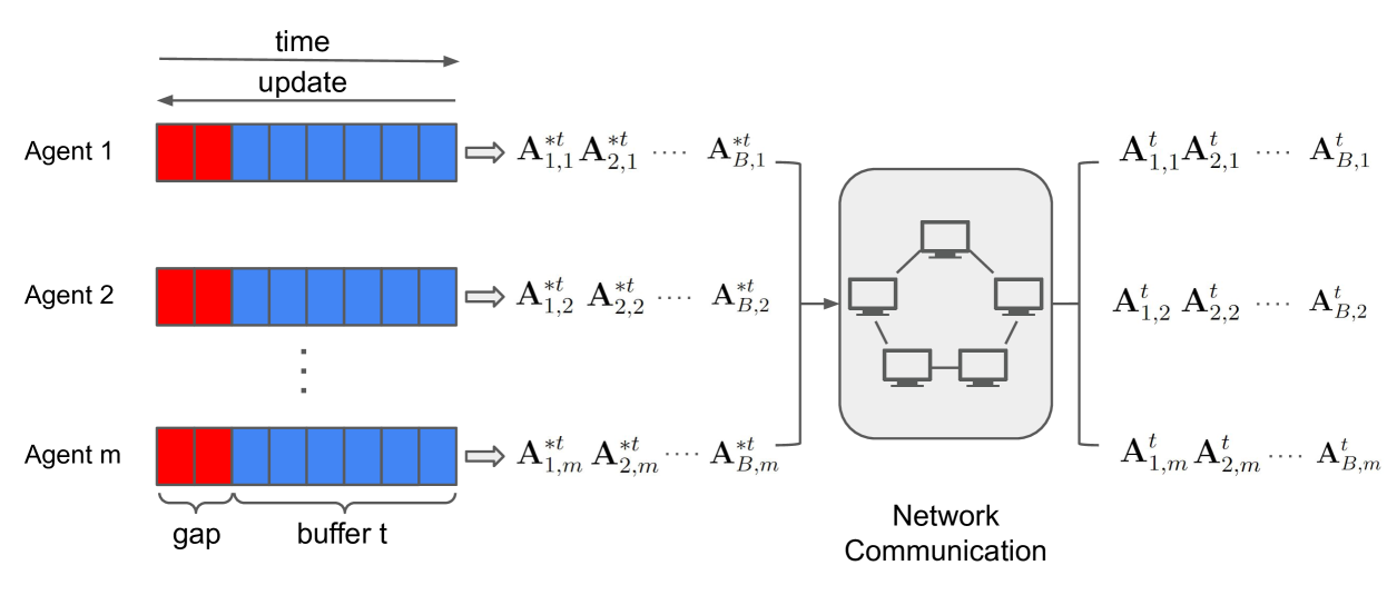
Figure 1: The illustration of the update scheme within one buffer: each agent splits the received data sequence into buffers and applies SGD reversely within each buffer. The estimate of each agent is then updated locally through the network communication. The communication between agents is based on the network structure captured by $\mathbf{P}.$

III Algorithm and Theoretical Results

We now lay out the distributed online linear system identification algorithm and provide the theoretical bound for the estimation error.

III-A Offline and Online Settings

For the identification of LTI systems, it is well-known that the (centralized) OLS estimator $\mathbf{A}_{OLS}:=\text{argmin}_{\mathbf{A}}\sum_{t=0}^{T-1}\left\lVert\mathbf{A}\mathbf{x}_{t}-\mathbf{x}_{t+1}\right\rVert^{2}$ is statistically optimal. OLS is an offline estimator that can also be implemented in an online fashion (i.e., in the form of recursive least squares) by keeping track of the data covariance matrix and the residual based on the current estimate. On the other hand, gradient-based methods provide efficient mechanisms for system identification. In particular, SGD uses the gradient of the current data pair $(\mathbf{x}_{t+1},\mathbf{x}_{t})$ to perform the update

$$\mathbf{A}_{t+1}=\mathbf{A}_{t}-2\gamma(\mathbf{A}_{t}\mathbf{x}_{t}-\mathbf{x}_{t+1})\mathbf{x}_{t}^{\top},$$

where $\gamma$ is the step size. Despite the efficient update, SGD suffers from the time-dependency over the data sequence, which leads to biased estimators. To observe this, unrolling the recursive update rule of SGD, we have

$$\begin{split}\mathbf{A}_{t}-\mathbf{A}&=(\mathbf{A}_{0}-\mathbf{A})\Pi_{s=0}^{t-1}(\mathbf{I}-2\gamma\mathbf{x}_{s}\mathbf{x}_{s}^{\top})\\ &+2\gamma\sum_{s=0}^{t-1}\mathbf{w}_{s}\mathbf{x}_{s}^{\top}\Pi_{l=s+1}^{t-1}(\mathbf{I}-2\gamma\mathbf{x}_{l}\mathbf{x}_{l}^{\top}),\end{split}$$

where in the second term, the dependence of later states on previous noise realizations prevents the estimator from being unbiased even if $\mathbf{A}_{0}$ is initialized with a distribution where $\mathrm{E}[\mathbf{A}_{0}]=\mathbf{A}$. To deal with this issue, [10] develops the method SGD-RER, which applies SGD in the reverse order of the sequence to break the dependency over time. Suppose that the estimate is updated along the opposite direction of the sequence. In particular, if we have $T$ samples and use the SGD update in the reverse order, the problematic term in the above equation takes the following form

$$2\gamma\sum_{k=0}^{t-1}\mathbf{w}_{T-k}\mathbf{x}_{T-k}^{\top}\Pi_{l=k+1}^{t-1}(\mathbf{I}-2\gamma\mathbf{x}_{T-l}\mathbf{x}_{T-l}^{\top}).$$

whose expectation is equal to zero since the later noise realizations are independent of previous states. Evidently, this approach does not work in an online sense (as the entire sequence of $T$ samples has to be collected first). However, we can mimic this approach by dividing the data into smaller buffers and use reverse SGD for each buffer [10].

III-B Distributed SGD with Reverse Experience Replay

We extend SGD-RER to the distributed case and call it the DSGD-RER algorithm. Each agent splits the sequence of data pairs into several buffers of size $B$, and within each buffer all agents perform SGD in the reverse order collectively based on the network topology. Between two consecutive buffers, $u$ data pairs are discarded in order to decrease the correlation of data in different buffers. The proposed method is outlined in Algorithm 1 and depicted in Fig. 1.

Averaged Iterate over Buffers: To further improve the convergence rate, we average the iterates. Each agent computes as the estimation output the tail-averaged estimate, i.e., the average of the last estimates of all buffers (line 11 of Algorithm 1).

Coupled Process: Despite the gap between buffers, there is still dependency across data points in various buffers, which makes the analysis challenging. To simplify the analysis, we consider the idea of coupled process [10], where for the state sequence $\{\mathbf{x}^{k}_{i}:i=0,\ldots,T\}$ received by agent $k$, the corresponding coupled sequence $\tilde{\mathbf{x}}^{k}_{i}$ is defined as follows.

1. For each buffer $t$, the starting state $\mathbf{x}^{k,t}_{0}$ is independently generated from $\pi$, the stationary distribution of the state.

2. The coupled process evolves according to the noise sequence $\mathbf{w}^{k,t}_{i}$ of the actual process, such that

   $$\tilde{\mathbf{x}}^{k,t}_{i+1}=\mathbf{A}\tilde{\mathbf{x}}^{k,t}_{i}+\mathbf{w}^{k,t}_{i},\>i=0,\ldots,S-1\>(S=B+u).$$

We will see in the analysis that it is more straightforward to first compute the estimation error based on the coupled process and then quantify the excessive error introduced by replacing the coupled process with the actual one. Note that based on the dynamics of the coupled process, the excessive error is related to the gap size $u$.

Algorithm 1 DSGD-RER

1:  Require: number of agents $m$, doubly stochastic matrix $\mathbf{P}\in\mathrm{R}^{m\times m}$, step size $\gamma$, buffer size $B$, gap size $u$, time horizon $T$, the parameter $\tau$.

2:  Initialize: $\mathbf{A}^{0}_{0,k}$ is initialized as a zero matrix for all agents $k\in[m]$. The number of buffers $N=T/S$, where $S=B+u$.

3:  for $t=0,1,\ldots,N-1$ do

4:     Each agent $k$ collects its data sequence of buffer $t$, $\{\mathbf{x}^{k,t}_{0},\mathbf{x}^{k,t}_{1},\ldots,\mathbf{x}^{k,t}_{S-1}\}$, where $\mathbf{x}^{k,t}_{i}:=\mathbf{x}^{k}_{S\cdot t+i}$, and we also define $\mathbf{x}^{k,t}_{-i}:=\mathbf{x}^{k,t}_{(S-1)-i}$.

5:     for $i=0,1,\ldots,B-1$ do

6:        for $k=1,2\ldots,m$ do

7:           $\mathbf{A}^{*t}_{i+1,k}=\mathbf{A}^{t}_{i,k}-2\gamma(\mathbf{A}^{t}_{i,k}\mathbf{x}^{k,t}_{-i}-\mathbf{x}^{k,t}_{-(i-1)}){(\mathbf{x}^{k,t}_{-i})}^{\top}$

8:        end for

9:        Each agent $k$ communicates with its neighbors based on $\mathbf{P}$ to update its estimate:

$$\mathbf{A}^{t}_{i+1,k}=\sum_{j\in\mathcal{N}_{i}}[\mathbf{P}{{}^{\tau}}]_{jk}\mathbf{A}^{*t}_{i+1,j}.$$

10:     end for

11:     For each agent $k$, compute the tail-averaged estimate until the current buffer as $\hat{\mathbf{A}}^{k}_{0,t}=\frac{1}{t+1}\sum_{s=0}^{t}\mathbf{A}^{s}_{B,k}$ and define $\mathbf{A}^{t+1}_{0,k}=\mathbf{A}^{t}_{B,k}$.

12:  end for

III-C Theoretical Guarantee

In this section, we present our main theoretical result. By running Algorithm 1 with specified hyper-parameters, we show that for the estimation error upper bound (of any agent), the term corresponding to the leading term in [10] can be improved by increasing the network size. There exists a (high probability) upper bound $R$ for the norm of state, such that $\left\lVert\mathbf{x}^{k,t}_{i}\right\rVert\leq\sqrt{R}$, which is also one of the parameters to be tuned.

Theorem 1

Let Assumptions 1-2 hold and consider the following hyper-parameter setup:

1. $d\leq O(\log(T))$.

2. $\gamma RB<\frac{1}{8}$.

3. $c_{1}\gamma B\sigma_{\min}(\mathbf{G})\leq\frac{1}{2}$, where $c_{1}$ is a problem-dependent constant.

4. $R=\Omega(C_{\mu}\sigma_{\max}(\mathbf{G})\log(T)),\\ B=u=\Theta(\sqrt{\frac{T}{\log(T)}}),\\ \gamma=\Theta(\frac{1}{\sqrt{T\log T}}\frac{\log\sqrt{T\log(T)}}{\log(T)}),\text{ and}\\ \tau=\Theta(\log(T))$.

Then, by applying Algorithm 1, with probability at least $1-(\frac{5m}{T^{\rho}}+\frac{3}{T^{v}})$ where $\rho$ and $v$ are some positive constants, the estimation error of the tail-averaged estimate of agent $k\in[m]$ over all buffers is bounded as follows

$$\begin{split}&\left\lVert\hat{\mathbf{A}}^{k}_{0,N-1}-\mathbf{A}\right\rVert\\ \leq&2\sqrt{m}\beta^{\tau}\gamma RT^{2}+(16\gamma^{2}R^{2}T^{2}+8\gamma RT)\left\lVert\mathbf{A}^{u}\right\rVert\\ +&\sqrt{\frac{8\gamma C_{\mu}\sigma_{\max}(\Sigma)(c_{6}d+v\log T)(1+2\alpha)}{Nm}}+\frac{\zeta\left\lVert\mathbf{A}_{0}-\mathbf{A}\right\rVert}{N}\\ +&\frac{4\left\lVert\mathbf{A}_{0}-\mathbf{A}\right\rVert}{c_{1}\gamma\sigma_{\min}(\mathbf{G})NB}\exp\big{(}-\frac{c_{1}\gamma B\sigma_{\min}(\mathbf{G})}{2}(\lceil\zeta\rceil+1)\big{)},\end{split}$$ (1)

where $\zeta:=\max\{\frac{c_{4}d}{c_{3}}+\log(NT^{v})/c_{3}-1,c_{2}\}$, $\alpha:=c_{5}(\zeta+\frac{1}{\gamma B\sigma_{\min}(\mathbf{G})})$ and $c_{1},\ldots,c_{5}$ are constants.

Remark 1

Comparing (1) and the estimation error upper bound of the centralized SGD-RER in [10], we can observe that for the dominant term in [10], the corresponding term in (1) is $\sqrt{\frac{8\gamma C_{\mu}\sigma_{\max}(\Sigma)(c_{6}d+v\log T)(1+2\alpha)}{Nm}}$, which shows that the contributed error can be improved by increasing the network size $m$.

IV Numerical Experiments

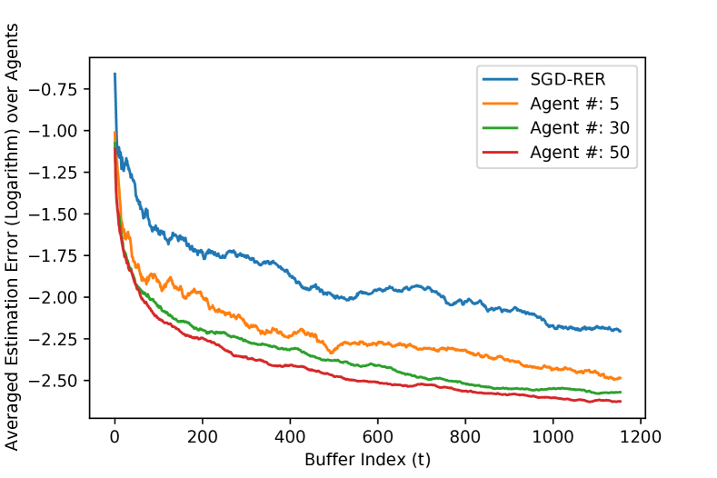
Figure 2: The plot shows that the estimation error of DSGD-RER improves as the network size increases. Also, DSGD-RER outperforms it centralized counter part SGD-RER.

Experiment Setup: We consider a network of LTI systems, where the transition matrix $\mathbf{A}\in\mathrm{R}^{d\times d}$ has the form $\mathbf{U}\Lambda\mathbf{U}^{\top}$. $\mathbf{U}$ is a randomly generated orthogonal matrix and $\Lambda$ is a diagonal matrix with two of its diagonal entries equal to $0.9$ and the rest equal to $0.3$. For the step size, we set $\gamma_{k}=\frac{1}{2R_{k}}$, where $R_{k}$ is estimated as the sum of the norms of the first $\lfloor 2\log T\rfloor$ samples of agent $k$. We also set the other hyper-parameters as follows: $T=10^{7}$, $u=\sqrt{\frac{T}{\log T}}$, $B=10u$, $\tau=1$ and $d=5$. The starting state $\mathbf{x}^{k}_{0}=0$, and the noise follows the standard Gaussian distribution $\mathcal{N}(0,\mathbf{I})$ $\forall k\in[m]$.

Networks: We examine the dependence of the estimation error to 1) the network size and 2) the network topology. For the former, we consider the centralized SGD-RER [10] and our distributed algorithm for $2$-cyclic graph with various agent numbers $m\in\{5,30,50\}$. For the latter, we look at the performance of a $5$-agent network with the following topologies: a) $\mathbf{P}=\mathbf{I}$ (Net A), fully disconnected; b) $\mathbf{P}$ captures a $2$-cyclic graph, where each agent has a self-weight of $0.3$ and assigns the weight of $0.35$ to each of its two neighbors (Net B); c) $\mathbf{P}=\frac{1}{m}{\mathbf{1}}{\mathbf{1}}^{\top}$ (Net C), the fully connected network.

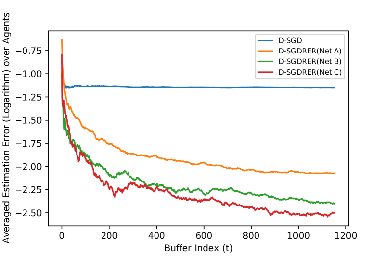
Figure 3: The averaged estimation error over time for different network topologies. The better the network is connected, the lower the estimation error is. Vanilla D-SGD (even in a fully connected network) is not competitive due to the correlation of data points.

Performance: From Fig. 2, we verify the dependency of the estimation precision on the network size. For a larger network size, the error of the tail-averaged estimate is smaller. Furthermore, all decentralized schemes outperform centralized SGD-RER [10]. To see the influence of network topology, notice that the value of $\beta$ for different networks is ordered as $\text{Net A}>\text{Net B}>\text{Net C}$. We can see in Fig. 3 that smaller $\beta$ results in a better estimation error. Furthermore, to see the impact of reverse estimation, we also plot the estimation error of applying vanilla distributed SGD in a fully connected network. We can see that the error does not shrink over time as the estimator is biased, so the reverse update process in DSGD-RER is critical.

V Conclusion

In this work, we considered the distributed online system identification problem for a network of identical LTI systems. We proposed a distributed online estimation algorithm and characterized the estimation error with respect to the network size and topology. We indeed observed in numerical experiments that larger network size as well as better connectivity can improve the estimation performance. For future directions, this online estimation method can be combined with decentralized control techniques to build decentralized, real-time adaptive controllers as explored in [23, 24]. Another potential direction is to extend the technique for identification of non-linear dynamical systems.

VI Appendix

For the complete proof of claims, see the longer version of the paper [25], where all necessary lemmas are included.

VI-A Notations and Proof Sketch

To analyze the distributed estimation error, we decompose it into two parts: (I) The estimation error from applying the fully-connected network $\mathbf{P}_{avg}=\frac{1}{m}{\mathbf{1}}{\mathbf{1}}^{\top}$ as the communication scheme; (II) The difference between estimates derived from $\mathbf{P}$ and $\mathbf{P}_{avg}$. To analyze (I), we apply the idea of coupled process: we consider $\tilde{\mathbf{A}}^{t,avg}_{i,k}$, agent $k$ estimate based on the coupled process and $\mathbf{P}_{avg}$. From the estimate initialization and the update scheme, we know $\tilde{\mathbf{A}}^{t,avg}_{i,1}=\tilde{\mathbf{A}}^{t,avg}_{i,2}=\cdots=\tilde{\mathbf{A}}^{t,avg}_{i,m}$, which we denote as $\tilde{\mathbf{A}}^{t,avg}_{i}$, coming with the recursive update rule:

$$\tilde{\mathbf{A}}^{t,avg}_{i+1}=\tilde{\mathbf{A}}^{t,avg}_{i}-\frac{2\gamma}{m}\sum_{k=1}^{m}(\tilde{\mathbf{A}}^{t,avg}_{i}\tilde{\mathbf{x}}^{k,t}_{-i}-\tilde{\mathbf{x}}^{k,t}_{-(i-1)})\tilde{\mathbf{x}}^{k,t\top}_{-i}.$$ (2)

We use the following notations for the rest of the proof:

$$\begin{split}\tilde{\mathbf{P}}^{t,avg}_{i}&:=\mathbf{I}-2\gamma\frac{\sum_{k=1}^{m}\tilde{\mathbf{x}}^{k,t}_{i}\tilde{\mathbf{x}}^{k,t\top}_{i}}{m},\\ \tilde{\mathbf{H}}^{t,avg}_{i,j}&:=\begin{cases}\prod_{s=i}^{j}\tilde{\mathbf{P}}^{t,avg}_{-s},\>&i\leq j\\ \mathbf{I},\>&i>j\end{cases}\end{split}$$

where the index $-j:=(S-1)-j$, and

$$\begin{split}\mathbf{x}^{k,t}_{-i}&:=\mathbf{x}^{k,t}_{(S-1)-i},\quad 0\leq i\leq S-1,\\ \mathcal{D}^{t}_{-j}&:=\Big{\{}\left\lVert\mathbf{x}^{k,t}_{-i}\right\rVert\leq\sqrt{R}:\>\forall k,\>j\leq i\leq B-1\Big{\}},\\ \tilde{\mathcal{D}}^{t}_{-j}&:=\Big{\{}\left\lVert\tilde{\mathbf{x}}^{k,t}_{-i}\right\rVert\leq\sqrt{R}:\>\forall k,\>j\leq i\leq B-1\Big{\}},\\ \mathcal{D}^{s,t}&:=\cap^{t}_{r=s}\mathcal{D}^{r}_{-0},\>s\leq t,\tilde{\mathcal{D}}^{s,t}:=\cap^{t}_{r=s}\tilde{\mathcal{D}}^{r}_{-0},\>s\leq t,\\ \hat{\mathcal{D}}^{s,t}&:=\mathcal{D}^{s,t}\cap\tilde{\mathcal{D}}^{s,t}.\end{split}$$

The estimate $\tilde{\mathbf{A}}^{avg}$ consists of a bias term and a variance term, which have the following expressions (see equations 18-19 in [10]):

$$\tilde{\mathbf{A}}^{t,avg}_{B}-\mathbf{A} =(\tilde{\mathbf{A}}^{t,avg}_{B,bias}-\mathbf{A})+\tilde{\mathbf{A}}^{t,avg}_{B,var},$$

$$(\tilde{\mathbf{A}}^{t,avg}_{B,bias}-\mathbf{A}) =(\mathbf{A}_{0}-\mathbf{A})\prod_{s=0}^{t}\tilde{\mathbf{H}}^{s,avg}_{0,B-1},$$

$$\begin{split}&\tilde{\mathbf{A}}^{t,avg}_{B,var}=\\ &2\gamma\sum_{r=0}^{t}\sum_{j=0}^{B-1}\big{(}\frac{\sum_{k=1}^{m}\mathbf{w}^{k,t-r}_{-j}\tilde{\mathbf{x}}^{k,t-r\top}_{-j}}{m}\big{)}\tilde{\mathbf{H}}^{t-r,avg}_{j+1,B-1}\prod_{s=r-1}^{0}\tilde{\mathbf{H}}^{t-s,avg}_{0,B-1}.\end{split}$$

VI-B Proof of the Main Theorem

First, we decompose the estimation error into several terms as follows:

$$\begin{split}&\left\lVert\hat{\mathbf{A}}^{k}_{0,N-1}-\mathbf{A}\right\rVert\\ \leq&\left\lVert\hat{\mathbf{A}}^{k}_{0,N-1}-\hat{\mathbf{A}}^{avg}_{0,N-1}\right\rVert+\left\lVert\hat{\mathbf{A}}^{avg}_{0,N-1}-\hat{\tilde{\mathbf{A}}}^{avg}_{0,N-1}\right\rVert\\ +&\left\lVert\hat{\tilde{\mathbf{A}}}^{var,avg}_{0,N-1}\right\rVert+\left\lVert\hat{\tilde{\mathbf{A}}}^{bias,avg}_{0,N-1}-\mathbf{A}\right\rVert.\end{split}$$ (3)

(I) For the term $\left\lVert\hat{\mathbf{A}}^{k}_{0,N-1}-\hat{\mathbf{A}}^{avg}_{0,N-1}\right\rVert$:
From Lemma 10, when the event of $\mathcal{D}^{0,N-1}$ holds, we have

$$\begin{split}\left\lVert\hat{\mathbf{A}}^{k}_{0,N-1}-\hat{\mathbf{A}}^{avg}_{0,N-1}\right\rVert&\leq\frac{1}{N}\sum_{t=0}^{N-1}\left\lVert\mathbf{A}^{t}_{B,k}-\mathbf{A}^{t,avg}_{B}\right\rVert\\ &\leq 2\sqrt{m}\beta^{\tau}\gamma RT^{2}.\end{split}$$

From Lemma 9 in [10], there exists a constant $\rho>0$ such that if $R=\Omega(C_{\mu}\sigma_{\max}(\mathbf{G})\log T)$, $\mathcal{P}(\mathcal{D}^{0,N-1})\geq 1-\frac{m}{T^{\rho}}$, from which we have

(II) For the term $\left\lVert\hat{\mathbf{A}}^{avg}_{0,N-1}-\hat{\tilde{\mathbf{A}}}^{avg}_{0,N-1}\right\rVert$:
Based on the expression of the tail-averaged estimate and Lemma 9, under the event of $\hat{\mathcal{D}}^{0,N-1}$, we have

$$\begin{split}\left\lVert\hat{\mathbf{A}}^{avg}_{0,N-1}-\hat{\tilde{\mathbf{A}}}^{avg}_{0,N-1}\right\rVert\leq&\frac{1}{N}\sum_{t=0}^{N-1}\left\lVert\mathbf{A}^{t,avg}_{B}-\tilde{\mathbf{A}}^{t,avg}_{B}\right\rVert\\ \leq&(16\gamma^{2}R^{2}T^{2}+8\gamma RT)\left\lVert\mathbf{A}^{u}\right\rVert.\end{split}$$

Based on Lemma 9 in [10], there exists a constant $\rho>0$ such that if $R=\Omega(C_{\mu}\sigma_{\max}(\mathbf{G})\log T)$, $\mathcal{P}(\hat{\mathcal{D}}^{0,N-1})\geq 1-\frac{2m}{T^{\rho}}$. Therefore, we conclude that

(III) For the term $\left\lVert\hat{\tilde{\mathbf{A}}}^{var,avg}_{0,N-1}\right\rVert$:
By applying Theorem 8 with the probability upper bound equal to $\frac{1}{T^{v}}$ where $v$ is some positive constant, we have that under the event of $\tilde{\mathcal{M}}^{0,N-1}\cap\tilde{\mathcal{D}}^{0,N-1}$ (the definition of $\tilde{\mathcal{M}}$ can be found in (16)), with probability at least $1-\frac{1}{T^{v}}$,

$$\left\lVert\hat{\tilde{\mathbf{A}}}^{var,avg}_{0,N-1}\right\rVert\leq\sqrt{\frac{8\gamma C_{\mu}\sigma_{\max}(\Sigma)(c_{6}d+v\log T)(1+2\alpha)}{Nm}}.$$ (6)

Based on Lemma 9 in [10], there exists a constant $\rho>0$ such that if $R=\Omega(C_{\mu}\sigma_{\max}(\mathbf{G})\log T)$, $\mathcal{P}(\tilde{\mathcal{D}}^{0,N-1})\geq 1-\frac{m}{T^{\rho}}$. Under the event of $\tilde{\mathcal{D}}^{0,N-1}$, by setting $\delta$ in Lemma 7 properly, we have

$$\mathcal{P}(\tilde{\mathcal{M}}^{0,N-1}\cap\tilde{\mathcal{D}}^{0,N-1})\geq 1-(\frac{1}{T^{v}}+\frac{m}{T^{\rho}}).$$

Combining above with (6), we conclude that

(IV) For the term $\left\lVert\hat{\tilde{\mathbf{A}}}^{bias,avg}_{0,N-1}-\mathbf{A}\right\rVert$:
Based on the expression of the bias term in Section VI-A, we have that

$$\begin{split}\left\lVert\hat{\tilde{\mathbf{A}}}^{bias,avg}_{0,N-1}-\mathbf{A}\right\rVert=&\left\lVert\frac{1}{N}\sum_{t=0}^{N-1}(\tilde{\mathbf{A}}^{t,avg}_{B,bias}-\mathbf{A})\right\rVert\\ \leq&\frac{\left\lVert\mathbf{A}_{0}-\mathbf{A}\right\rVert}{N}\sum_{t=0}^{N-1}\left\lVert\prod_{s=0}^{t}\tilde{\mathbf{H}}^{s,avg}_{0,B-1}\right\rVert.\end{split}$$ (8)

From the result of Lemma 6 with $\zeta:=\max\{\frac{c_{4}d}{c_{3}}+\log(\frac{N}{\delta})/c_{3}-1,c_{2}\}$, we have, for all $t\geq\zeta$

$$\left\lVert\prod_{s=0}^{t}\tilde{\mathbf{H}}^{s,avg}_{0,B-1}\right\rVert\leq 2\big{(}1-\gamma B\sigma_{\min}(\mathbf{G})\big{)}^{\frac{c_{1}}{2}(t+1)},$$ (9)

with probability at least $(1-\delta)$ under the event of $\tilde{\mathcal{D}}^{0,N-1}$. Based on Lemma 6, under the event of $\tilde{\mathcal{D}}^{0,N-1}$ we also have for all $t<\zeta$,

$$\left\lVert\prod_{s=0}^{t}\tilde{\mathbf{H}}^{s,avg}_{0,B-1}\right\rVert\leq 1\text{ almost surely}.$$ (10)

Based on (8), (9) and (10), we have, under the event of $\tilde{\mathcal{D}}^{0,N-1}$ with probability at least $(1-\delta)$,

By setting $\delta$ as $\frac{1}{T^{v}}$, based on (11) and the fact that $\mathcal{P}(\tilde{\mathcal{D}}^{0,N-1})\geq 1-\frac{m}{T^{\rho}}$, we have

Applying the results of (4), (5), (7) and (12) on (3), with probability at least $1-(\frac{5m}{T^{\rho}}+\frac{3}{T^{v}})$ we have

$$\begin{split}&\left\lVert\hat{\mathbf{A}}^{k}_{0,N-1}-\mathbf{A}\right\rVert\\ \leq&2\sqrt{m}\beta^{\tau}\gamma RT^{2}+(16\gamma^{2}R^{2}T^{2}+8\gamma RT)\left\lVert\mathbf{A}^{u}\right\rVert\\ +&\sqrt{\frac{8\gamma C_{\mu}\sigma_{\max}(\Sigma)(c_{6}d+v\log T)(1+2\alpha)}{Nm}}+\frac{\zeta\left\lVert\mathbf{A}_{0}-\mathbf{A}\right\rVert}{N}\\ +&\frac{4\left\lVert\mathbf{A}_{0}-\mathbf{A}\right\rVert}{c_{1}\gamma\sigma_{\min}(\mathbf{G})NB}\exp\big{(}-\frac{c_{1}\gamma B\sigma_{\min}(\mathbf{G})}{2}(\lceil\zeta\rceil+1)\big{)}.\end{split}$$ (13)

VII Supplementary Material

VII-A Bounds of the Estimation Error of $\tilde{\mathbf{A}}^{avg}$ and $\mathbf{A}^{avg}$

Lemma 2

Suppose that Assumption 2 and $\gamma R<1/2$ hold. Then, $\forall t\geq 0$ and for any $\lambda\in\mathrm{R}$ and $\mathbf{x},\mathbf{y}\in\mathrm{R}^{d}$, we have

$$\begin{split}&\mathrm{E}\big{[}\exp(\frac{\gamma}{m}\lambda^{2}C_{\mu}\mathbf{x}^{\top}\Sigma\mathbf{x}\langle\mathbf{y},\tilde{\mathbf{H}}^{t,avg\top}_{0,B-1}\tilde{\mathbf{H}}^{t,avg}_{0,B-1}\mathbf{y}\rangle+\lambda\mathbf{x}^{\top}\Delta^{t}\mathbf{y})|\tilde{\mathcal{D}}^{t}_{-0}\big{]}\\ \leq&\frac{\exp(\frac{\gamma}{m}\lambda^{2}C_{\mu}\mathbf{x}^{\top}\Sigma\mathbf{x}\left\lVert\mathbf{y}\right\rVert^{2})}{\mathcal{P}(\tilde{\mathcal{D}}^{t}_{-0})}.\end{split}$$

Proof:

For the ease of analysis, we have the following notations:

$$\begin{split}\Delta^{t}&:=2\gamma\sum_{j=0}^{B-1}\big{(}\frac{\sum_{k=1}^{m}\mathbf{w}^{k,t}_{-j}\tilde{\mathbf{x}}^{k,t\top}_{-j}}{m}\big{)}\tilde{\mathbf{H}}^{t,avg}_{j+1,B-1},\\ \Delta^{t}_{-i}&:=2\gamma\sum_{j=i}^{B-1}\big{(}\frac{\sum_{k=1}^{m}\mathbf{w}^{k,t}_{-j}\tilde{\mathbf{x}}^{k,t\top}_{-j}}{m}\big{)}\tilde{\mathbf{H}}^{t,avg}_{j+1,B-1},\\ \Xi^{t}_{0}&:=\frac{\gamma}{m}\lambda^{2}C_{\mu}\mathbf{x}^{\top}\Sigma\mathbf{x}\langle\mathbf{y},\tilde{\mathbf{H}}^{t,avg\top}_{0,B-1}\tilde{\mathbf{H}}^{t,avg}_{0,B-1}\mathbf{y}\rangle,\\ \Xi^{t}_{i}&:=\frac{\gamma}{m}\lambda^{2}C_{\mu}\mathbf{x}^{\top}\Sigma\mathbf{x}\langle\mathbf{y},\tilde{\mathbf{H}}^{t,avg\top}_{i,B-1}\tilde{\mathbf{H}}^{t,avg}_{i,B-1}\mathbf{y}\rangle.\end{split}$$

From the notation above and $\gamma R<1/2$, under the event $\tilde{\mathcal{D}}^{t}_{-0}$ we have

where the inequality is due to the following

$$\begin{split}&\tilde{\mathbf{P}}^{t,avg\top}_{-i}\tilde{\mathbf{P}}^{t,avg}_{-i}+\frac{2\gamma}{m}\sum_{k=1}^{m}(\tilde{\mathbf{x}}^{k,t}_{-i}\tilde{\mathbf{x}}^{k,t\top}_{-i})\\ =&\big{(}\mathbf{I}-\frac{2\gamma}{m}\sum_{k=1}^{m}\tilde{\mathbf{x}}^{k,t}_{-i}\tilde{\mathbf{x}}^{k,t\top}_{-i}+\frac{4\gamma^{2}}{m^{2}}\sum_{k=1}^{m}\sum_{s=1}^{m}\tilde{\mathbf{x}}^{k,t}_{-i}\tilde{\mathbf{x}}^{k,t\top}_{-i}\tilde{\mathbf{x}}^{s,t}_{-i}\tilde{\mathbf{x}}^{s,t\top}_{-i}\big{)}\\ \preceq&\left(\mathbf{I}-\frac{2\gamma}{m}\sum_{k=1}^{m}\tilde{\mathbf{x}}^{k,t}_{-i}\tilde{\mathbf{x}}^{k,t\top}_{-i}+\frac{4\gamma^{2}R}{m}\sum_{k=1}^{m}\tilde{\mathbf{x}}^{k,t}_{-i}\tilde{\mathbf{x}}^{k,t\top}_{-i}\right)\preceq\mathbf{I}.\end{split}$$

Knowing that $\Delta^{t}_{-i}=2\gamma\big{(}\frac{\sum_{k=1}^{m}\mathbf{w}^{k,t}_{-i}\tilde{\mathbf{x}}^{k,t\top}_{-i}}{m}\big{)}\tilde{\mathbf{H}}^{t,avg}_{i+1,B-1}+\Delta^{t}_{-(i+1)}$ and defining

we get

$$\begin{split}&\mathrm{E}\left[\exp(\Xi^{t}_{0}+\lambda\langle\mathbf{x},\Delta^{t}\mathbf{y}\rangle)\middle|\tilde{\mathcal{D}}^{t}_{-0}\right]\\ =&\frac{\mathrm{E}\left[\exp(\Xi^{t}_{0}+\lambda\langle\mathbf{x},\Delta^{t}_{-0}\mathbf{y}\rangle)\mathbf{1}(\tilde{\mathcal{D}}^{t}_{-0})\right]}{\mathcal{P}(\tilde{\mathcal{D}}^{t}_{-0})}\\ =&\frac{\mathrm{E}\left[\exp(\Xi^{t}_{0}+\lambda\langle\mathbf{x},(\Delta^{t}_{-0}-\Delta^{t}_{-1})\mathbf{y}\rangle+\lambda\langle\mathbf{x},\Delta^{t}_{-1}\mathbf{y}\rangle)\mathbf{1}(\tilde{\mathcal{D}}^{t}_{-0})\right]}{\mathcal{P}(\tilde{\mathcal{D}}^{t}_{-0})}\\ \leq&\frac{\mathrm{E}\left[\exp\left(\Xi^{t}_{0}+\varkappa^{t}_{0}+\lambda\langle\mathbf{x},\Delta^{t}_{-1}\mathbf{y}\rangle\right)\mathbf{1}(\tilde{\mathcal{D}}^{t}_{-0})\right]}{\mathcal{P}(\tilde{\mathcal{D}}^{t}_{-0})}\\ \leq&\frac{\mathrm{E}\left[\exp(\Xi^{t}_{1}+\lambda\langle\mathbf{x},\Delta^{t}_{-1}\mathbf{y}\rangle)\mathbf{1}(\tilde{\mathcal{D}}^{t}_{-0})\right]}{\mathcal{P}(\tilde{\mathcal{D}}^{t}_{-0})}\\ \leq&\frac{\mathrm{E}\left[\exp(\Xi^{t}_{1}+\lambda\langle\mathbf{x},\Delta^{t}_{-1}\mathbf{y}\rangle)\mathbf{1}(\tilde{\mathcal{D}}^{t}_{-1})\right]}{\mathcal{P}(\tilde{\mathcal{D}}^{t}_{-0})},\end{split}$$ (15)

where the first inequality is due to the sub-Gaussianity of $\langle\mathbf{x},\mathbf{w}^{k,t}_{-0}\rangle$ and the fact that $\forall k\in[m]$, $\mathbf{w}^{k,t}_{-0}$ is independent of $\Xi^{t}_{0}$, $\tilde{\mathbf{H}}^{t,avg}_{1,B-1}$, $\Delta^{t}_{-1}$ and $\tilde{\mathcal{D}}^{t}_{-0}$, the second inequality comes from (14), and the last inequality is based on $\tilde{\mathcal{D}}^{t}_{-0}\subseteq\tilde{\mathcal{D}}^{t}_{-1}$. Then, by expanding the recursive relationship in (15), the result is proved. ∎

Corollary 3

From Lemma 2, we have

$$\begin{split}\mathrm{E}\big{[}\exp(\lambda\mathbf{x}^{\top}\Delta^{t}\mathbf{y})|\tilde{\mathcal{D}}^{t}_{-0}\big{]}\leq\frac{\exp(\frac{\gamma}{m}\lambda^{2}C_{\mu}\mathbf{x}^{\top}\Sigma\mathbf{x}\left\lVert\mathbf{y}\right\rVert^{2})}{\mathcal{P}(\tilde{\mathcal{D}}^{t}_{-0})}.\end{split}$$

Lemma 4

Suppose that $\gamma BR<\frac{1}{6}$. Then, under $\tilde{D}^{t}_{-0}\>\forall t$ the following relationships hold:

$$\begin{split}&\mathbf{I}-4\gamma\left(1+\frac{2\gamma BR}{1-4\gamma BR}\right)\sum_{i=0}^{B-1}\sum_{k=1}^{m}\tilde{\mathbf{x}}^{k,t}_{-i}\tilde{\mathbf{x}}^{k,t\top}_{-i}\preceq\tilde{\mathbf{H}}^{t,avg\top}_{0,B-1}\tilde{\mathbf{H}}^{t,avg}_{0,B-1}\\ &\tilde{\mathbf{H}}^{t,avg\top}_{0,B-1}\tilde{\mathbf{H}}^{t,avg}_{0,B-1}\preceq\mathbf{I}-4\gamma\left(1-\frac{2\gamma BR}{1-4\gamma BR}\right)\sum_{i=0}^{B-1}\sum_{k=1}^{m}\tilde{\mathbf{x}}^{k,t}_{-i}\tilde{\mathbf{x}}^{k,t\top}_{-i}.\end{split}$$

Proof:

The result can be derived by following the proof of Lemma 28 in [10]. ∎

Lemma 5

Suppose that $\gamma RB<\frac{1}{8}$, Assumption 2 holds, and there exists a constant $c_{0}>0$ such that $c_{0}<\frac{1}{128C_{\mu}^{2}}$ and $1-c_{0}\leq\mathcal{P}(\tilde{\mathcal{D}}^{t}_{-0})$. Then, for any $\mathbf{x}\in\mathrm{R}^{d}$ we get

$$\mathcal{P}\left(\left\lVert\tilde{\mathbf{H}}^{t,avg}_{0,B-1}\mathbf{x}\right\rVert^{2}\geq\left\lVert\mathbf{x}\right\rVert^{2}-B\gamma\mathbf{x}^{\top}\mathbf{G}\mathbf{x}\middle|\tilde{\mathcal{D}}^{t}_{-0}\right)\leq 1-p_{0},$$

where $p_{0}:=\frac{1}{1-c_{0}}(\frac{1}{128C_{\mu}^{2}}-c_{0})$.

Proof:

The result can be derived using Lemma 4 and the proof of Lemma 30 in [10]. ∎

Lemma 6

Suppose that the conditions in Lemma 5 hold and there exists a constant $c_{1}>0$, such that $c_{1}<e(1-p_{0})<(1-c_{1})$ and $b-a>c_{2}:=\frac{e(1-p_{0})-c_{1}}{(1-c_{1})-e(1-p_{0})}$. Then, conditioned on $\tilde{\mathcal{D}}^{a,b}$, we have

1. $\left\lVert\prod_{s=a}^{b}\tilde{\mathbf{H}}^{s,avg}_{0,B-1}\right\rVert\leq 1$ almost surely.

2. $\mathcal{P}\left(\left\lVert\prod_{s=a}^{b}\tilde{\mathbf{H}}^{s,avg}_{0,B-1}\right\rVert\geq 2(1-\gamma B\sigma_{\min}(\mathbf{G}))^{\frac{c_{1}}{2}(b-a+1)}\right)\\ \leq\exp(-c_{3}(b-a+1)+c_{4}d)$, where $c_{3},c_{4}$ are constants, and $c_{3}$ depends on $C_{\mu}$.

Proof:

The result can be derived by following the proof of Lemma 31 in [10]. ∎

Let us now define $F_{a,N-1}:=\sum_{r=a}^{N-1}\prod_{s=a+1}^{r}\tilde{\mathbf{H}}^{s,avg\top}_{0,B-1}$.

Lemma 7

Suppose that $c_{1}\gamma B\sigma_{\min}(\mathbf{G})<\frac{1}{2}$ and the conditions in Lemma 6 hold. Then, for any $\delta\in(0,1)$, we have

$$\mathcal{P}\left(\left\lVert F_{a,N-1}\right\rVert\geq c_{5}\big{(}\zeta+\frac{1}{\gamma B\sigma_{\min}(\mathbf{G})}\big{)}\middle|\tilde{\mathcal{D}}^{a,N-1}\right)\leq\delta,$$

where $\zeta:=\max\{\frac{c_{4}d}{c_{3}}+\log(\frac{N}{\delta})/c_{3}-1,c_{2}\}$, and $c_{5}$ is a constant depending on $C_{\mu}$.

Consider the tail-averaged estimate:

$$\begin{split}\hat{\tilde{\mathbf{A}}}^{var,avg}_{0,N-1}&=\frac{1}{N}\sum_{t=0}^{N-1}(\tilde{\mathbf{A}}^{t,avg}_{B,var})=\frac{1}{N}\sum_{t=0}^{N-1}\Delta^{t}F_{t,N-1}.\end{split}$$

Define the following events:

$$\begin{split}\tilde{\mathcal{M}}^{t}&:=\left\{\left\lVert F_{t,N-1}\right\rVert\leq c_{5}(\zeta+\frac{1}{\gamma B\sigma_{\min}}(\mathbf{G}))\right\},\\ \tilde{\mathcal{M}}^{t,N-1}&:=\cap_{s=t}^{N-1}\tilde{\mathcal{M}}^{s}.\end{split}$$ (16)

Theorem 8

Suppose that the conditions in Lemma 2, Lemma 4 and Lemma 7 hold. Assume $\mathcal{P}(\tilde{\mathcal{M}}^{0,N-1}\cap\tilde{\mathcal{D}}^{0,N-1})\geq\frac{1}{2}$ and define $\alpha:=c_{5}(\zeta+\frac{1}{\gamma B\sigma_{\min}(\mathbf{G})})$. Then we have

$$\begin{split}&\mathcal{P}\left(\left\lVert\hat{\tilde{\mathbf{A}}}^{var,avg}_{0,N-1}\right\rVert\geq\beta^{\prime}\middle|\tilde{\mathcal{M}}^{0,N-1}\cap\tilde{\mathcal{D}}^{0,N-1}\right)\\ \leq&\exp(c_{6}d-\frac{\beta^{\prime 2}Nm}{8\gamma C_{\mu}\sigma_{\max}(\Sigma)(1+2\alpha)}),\end{split}$$

where $c_{6}$ is a problem-independent constant.

Proof:

The result can be derived by following the proof of Theorem 33 in [10]. ∎

Lemma 9

Suppose that $2\gamma R<1$ and the event of $\hat{\mathcal{D}}^{0,N-1}$ holds. Then, for $0\leq t\leq N-1$ and $0\leq i\leq B-1$, we have

$$\left\lVert\mathbf{A}^{t,avg}_{i}-\tilde{\mathbf{A}}^{t,avg}_{i}\right\rVert\leq(16\gamma^{2}R^{2}T^{2}+8\gamma RT)\left\lVert\mathbf{A}^{u}\right\rVert.$$

Proof:

Consider the update rule of $\mathbf{A}^{t,avg}_{i},\>0\leq i\leq B-1$:

$$\begin{split}\mathbf{A}^{t,avg}_{i+1}&=\mathbf{A}^{t,avg}_{i}-\frac{2\gamma}{m}\sum_{k=1}^{m}(\mathbf{A}^{t,avg}_{i}\mathbf{x}^{k,t}_{-i}-\mathbf{x}^{k,t}_{-(i-1)})\mathbf{x}^{k,t\top}_{-i}\\ &=\mathbf{A}^{t,avg}_{i}-\frac{2\gamma}{m}\sum_{k=1}^{m}(\mathbf{A}^{t,avg}_{i}\tilde{\mathbf{x}}^{k,t}_{-i}-\tilde{\mathbf{x}}^{k,t}_{-(i-1)})\tilde{\mathbf{x}}^{k,t\top}_{-i}\\ &+\frac{2\gamma}{m}\sum_{k=1}^{m}\mathbf{A}^{t,avg}_{i}\left(\tilde{\mathbf{x}}^{k,t}_{-i}\tilde{\mathbf{x}}^{k,t\top}_{-i}-\mathbf{x}^{k,t}_{-i}\mathbf{x}^{k,t\top}_{-i}\right)\\ &+\frac{2\gamma}{m}\sum_{k=1}^{m}\left(\mathbf{x}^{k,t}_{-(i-1)}\mathbf{x}^{k,t\top}_{-i}-\tilde{\mathbf{x}}^{k,t}_{-(i-1)}\tilde{\mathbf{x}}^{k,t\top}_{-i}\right).\end{split}$$ (17)

Combining above with (2), we obtain

$$\begin{split}\mathbf{A}^{t,avg}_{i+1}-\tilde{\mathbf{A}}^{t,avg}_{i+1}&=(\mathbf{A}^{t,avg}_{i}-\tilde{\mathbf{A}}^{t,avg}_{i})\tilde{\mathbf{P}}^{t,avg}_{-i}\\ &+\frac{2\gamma}{m}\sum_{k=1}^{m}\mathbf{A}^{t,avg}_{i}\left(\tilde{\mathbf{x}}^{k,t}_{-i}\tilde{\mathbf{x}}^{k,t\top}_{-i}-\mathbf{x}^{k,t}_{-i}\mathbf{x}^{k,t\top}_{-i}\right)\\ &+\frac{2\gamma}{m}\sum_{k=1}^{m}\left(\mathbf{x}^{k,t}_{-(i-1)}\mathbf{x}^{k,t\top}_{-i}-\tilde{\mathbf{x}}^{k,t}_{-(i-1)}\tilde{\mathbf{x}}^{k,t\top}_{-i}\right).\end{split}$$ (18)

For the term $\mathbf{A}^{t,avg}_{i}$, based on the update rule, the choice of $\gamma$ and the condition of $\hat{\mathcal{D}}^{0,N-1}$, we have

$$\begin{split}\left\lVert\mathbf{A}^{t,avg}_{i+1}\right\rVert&=\left\lVert\mathbf{A}^{t,avg}_{i}\mathbf{P}^{t,avg}_{-i}+\frac{2\gamma}{m}\sum_{k=1}^{m}\mathbf{x}^{k,t}_{-(i-1)}\mathbf{x}^{k,t\top}_{-i}\right\rVert\\ &\leq\left\lVert\mathbf{A}^{t,avg}_{i}\right\rVert\left\lVert\mathbf{P}^{t,avg}_{-i}\right\rVert+\frac{2\gamma}{m}\sum_{k=1}^{m}\left\lVert\mathbf{x}^{k,t}_{-(i-1)}\mathbf{x}^{k,t\top}_{-i}\right\rVert\\ &\leq\left\lVert\mathbf{A}^{t,avg}_{i}\right\rVert+2\gamma R,\end{split}$$

from which we conclude that for $0\leq t\leq N-1$ and $0\leq i\leq B-1$,

$$\left\lVert\mathbf{A}^{t,avg}_{i}\right\rVert\leq 2\gamma RT.$$ (19)

For the term $\left(\tilde{\mathbf{x}}^{k,t}_{-i}\tilde{\mathbf{x}}^{k,t\top}_{-i}-\mathbf{x}^{k,t}_{-i}\mathbf{x}^{k,t\top}_{-i}\right)$, it can be shown that

$$\begin{split}&\left\lVert\tilde{\mathbf{x}}^{k,t}_{-i}\tilde{\mathbf{x}}^{k,t\top}_{-i}-\mathbf{x}^{k,t}_{-i}\mathbf{x}^{k,t\top}_{-i}\right\rVert\\ =&\left\lVert\tilde{\mathbf{x}}^{k,t}_{-i}\tilde{\mathbf{x}}^{k,t\top}_{-i}-\mathbf{x}^{k,t}_{-i}\tilde{\mathbf{x}}^{k,t\top}_{-i}+\mathbf{x}^{k,t}_{-i}\tilde{\mathbf{x}}^{k,t\top}_{-i}-\mathbf{x}^{k,t}_{-i}\mathbf{x}^{k,t\top}_{-i}\right\rVert\\ \leq&2\sqrt{R}\left\lVert\mathbf{x}^{k,t}_{-i}-\tilde{\mathbf{x}}^{k,t}_{-i}\right\rVert=2\sqrt{R}\left\lVert\mathbf{A}^{(S-1)-i}(\mathbf{x}^{k,t}_{0}-\tilde{\mathbf{x}}^{k,t}_{0})\right\rVert\\ \leq&4R\left\lVert\mathbf{A}^{u}\right\rVert,\end{split}$$ (20)

where the first inequality is due to the condition of $\hat{\mathcal{D}}^{0,N-1}$ and the last inequality comes from the gap between buffers. Similarly, we can show $\left\lVert\mathbf{x}^{k,t}_{-(i-1)}\mathbf{x}^{k,t\top}_{-i}-\tilde{\mathbf{x}}^{k,t}_{-(i-1)}\tilde{\mathbf{x}}^{k,t\top}_{-i}\right\rVert\leq 4R\left\lVert\mathbf{A}^{u}\right\rVert$.

Substituting (19) and (20) into (18), we get

$$\begin{split}&\left\lVert\mathbf{A}^{t,avg}_{i+1}-\tilde{\mathbf{A}}^{t,avg}_{i+1}\right\rVert\\ \leq&\left\lVert\mathbf{A}^{t,avg}_{i}-\tilde{\mathbf{A}}^{t,avg}_{i}\right\rVert\left\lVert\tilde{\mathbf{P}}^{t,avg}_{-i}\right\rVert+(16\gamma^{2}R^{2}T+8\gamma R)\left\lVert\mathbf{A}^{u}\right\rVert\\ \leq&\left\lVert\mathbf{A}^{t,avg}_{i}-\tilde{\mathbf{A}}^{t,avg}_{i}\right\rVert+(16\gamma^{2}R^{2}T+8\gamma R)\left\lVert\mathbf{A}^{u}\right\rVert,\end{split}$$

from which we conclude that for $0\leq t\leq N-1$ and $0\leq i\leq B-1$,

$$\left\lVert\mathbf{A}^{t,avg}_{i}-\tilde{\mathbf{A}}^{t,avg}_{i}\right\rVert\leq(16\gamma^{2}R^{2}T^{2}+8\gamma RT)\left\lVert\mathbf{A}^{u}\right\rVert.$$

∎

VII-B Difference between $\mathbf{A}^{t}_{i,k}$ and $\mathbf{A}^{t,avg}_{i}$

Lemma 10

Suppose that $2\gamma R<1$ and the event of $\mathcal{D}^{0,N-1}$ holds. Then, for $0\leq t\leq N-1$ and $0\leq i\leq B-1$, we have for any agent $k$

$$\left\lVert\mathbf{A}^{t}_{i,k}-\mathbf{A}^{t,avg}_{i}\right\rVert\leq 2\sqrt{m}\beta^{\tau}\gamma RT^{2}.$$

Proof:

First, we note that using the recursive relationship (19), it is easy to verify that under the condition of $\mathcal{D}^{0,N-1}$, both $\left\lVert\mathbf{A}^{*t}_{i,k}\right\rVert$ and $\left\lVert\mathbf{A}^{t,avg}_{i}\right\rVert$ are upper-bounded by $2(S*t+i)\gamma R$. Let us define the following notations:

$$\begin{split}\bar{\mathbf{A}}^{t}_{i}&:=\frac{1}{m}\sum_{k=1}^{m}\mathbf{A}^{*t}_{i,k},\\ \mathbf{e}^{t}_{i,k}&:=\mathbf{A}^{t}_{i,k}-\mathbf{A}^{t,avg}_{i},\;\text{and }\left\lVert\mathbf{e}^{t}_{i,k}\right\rVert\leq E^{t}_{i}\;\forall k.\end{split}$$

With Algorithm 1, we have the following update expressions:

$$\mathbf{A}^{t,avg}_{i+1}=\mathbf{A}^{t,avg}_{i}-\frac{2\gamma}{m}\sum_{k=1}^{m}(\mathbf{A}^{t,avg}_{i}\mathbf{x}^{k,t}_{-i}-\mathbf{x}^{k,t}_{-(i-1)})\mathbf{x}^{k,t\top}_{-i},$$ (21)

and

$$\mathbf{A}^{*t}_{i+1,k}=\mathbf{A}^{t}_{i,k}-2\gamma(\mathbf{A}^{t}_{i,k}\mathbf{x}^{k,t}_{-i}-\mathbf{x}^{k,t}_{-(i-1)}){(\mathbf{x}^{k,t}_{-i})}^{\top}.$$ (22)

Substituting $(\mathbf{A}^{t,avg}_{i}+\mathbf{e}^{t}_{i,k})$ for $\mathbf{A}^{t}_{i,k}$ in (22), with the definition of $\bar{\mathbf{A}}^{t}_{i+1}$, we get

$$\begin{split}\left\lVert\bar{\mathbf{A}}^{t}_{i+1}-\mathbf{A}^{t,avg}_{i+1}\right\rVert&=\left\lVert\frac{1}{m}\sum_{k=1}^{m}\mathbf{e}^{t}_{i,k}(\mathbf{I}-2\gamma\mathbf{x}^{k,t}_{-i}\mathbf{x}^{k,t\top}_{-i})\right\rVert\\ &\leq E^{t}_{i}.\end{split}$$ (23)

On the other hand, through step 9 in Algorithm 1, it can be shown that $\forall k$,

$$\begin{split}&\left\lVert\mathbf{A}^{t}_{i+1,k}-\bar{\mathbf{A}}^{t}_{i+1}\right\rVert\\ =&\left\lVert\sum_{j}[\mathbf{P}^{\tau}]_{jk}\mathbf{A}^{*t}_{i+1,j}-\frac{1}{m}\sum_{j}\mathbf{A}^{*t}_{i+1,j}\right\rVert\\ \leq&\sum_{j}\left|[\mathbf{P}^{\tau}]_{jk}-\frac{1}{m}\right|\left\lVert\mathbf{A}^{*t}_{i+1,j}\right\rVert\\ \leq&\sqrt{m}2(S*t+i+1)\beta^{\tau}\gamma R.\end{split}$$ (24)

With (23) and (24), the relationship between $E^{t}_{i+1}$ and $E^{t}_{i}$ is as follows:

$$\begin{split}&\left\lVert\mathbf{A}^{t}_{i+1,k}-\mathbf{A}^{t,avg}_{i+1}\right\rVert\\ \leq&\left\lVert\mathbf{A}^{t}_{i+1,k}-\bar{\mathbf{A}}^{t}_{i+1}\right\rVert+\left\lVert\bar{\mathbf{A}}^{t}_{i+1}-\mathbf{A}^{t,avg}_{i+1}\right\rVert\\ \leq&2\sqrt{m}(S*t+i+1)\beta^{\tau}\gamma R+E^{t}_{i}:=E^{t}_{i+1}.\end{split}$$ (25)

Notice that with the zero initialization of all agents estimates, it can be shown that $E^{0}_{1}=2\sqrt{m}\beta^{\tau}\gamma R$. Expanding (25) recursively, we get

$$\begin{split}E^{t}_{i}\leq&2\sqrt{m}\beta^{\tau}\gamma RT^{2}.\end{split}$$ (26)

∎

References

- [1] K. J. Åström and P. Eykhoff, “System identification—a survey,” Automatica, vol. 7, no. 2, pp. 123–162, 1971.
- [2] L. Ljung, “System identification,” Wiley encyclopedia of electrical and electronics engineering, pp. 1–19, 1999.
- [3] H.-F. Chen and L. Guo, Identification and stochastic adaptive control. Springer Science & Business Media, 2012.
- [4] G. C. Goodwin, G. GC, and P. RL, “Dynamic system identification. experiment design and data analysis.” 1977.
- [5] S. Dean, H. Mania, N. Matni, B. Recht, and S. Tu, “On the sample complexity of the linear quadratic regulator,” Foundations of Computational Mathematics, pp. 1–47, 2019.
- [6] Y. Jedra and A. Proutiere, “Finite-time identification of stable linear systems optimality of the least-squares estimator,” in 2020 59th IEEE Conference on Decision and Control (CDC). IEEE, 2020, pp. 996–1001.
- [7] M. K. S. Faradonbeh, A. Tewari, and G. Michailidis, “Finite time identification in unstable linear systems,” Automatica, vol. 96, pp. 342–353, 2018.
- [8] M. Simchowitz, H. Mania, S. Tu, M. I. Jordan, and B. Recht, “Learning without mixing: Towards a sharp analysis of linear system identification,” in Conference On Learning Theory. PMLR, 2018, pp. 439–473.
- [9] T. Sarkar and A. Rakhlin, “Near optimal finite time identification of arbitrary linear dynamical systems,” in International Conference on Machine Learning. PMLR, 2019, pp. 5610–5618.
- [10] S. Kowshik, D. Nagaraj, P. Jain, and P. Netrapalli, “Streaming linear system identification with reverse experience replay,” Advances in Neural Information Processing Systems, vol. 34, 2021.
- [11] Y. Jedra and A. Proutiere, “Sample complexity lower bounds for linear system identification,” in 2019 IEEE 58th Conference on Decision and Control (CDC). IEEE, 2019, pp. 2676–2681.
- [12] S. Oymak and N. Ozay, “Non-asymptotic identification of lti systems from a single trajectory,” in American control conference (ACC), 2019, pp. 5655–5661.
- [13] T. Sarkar, A. Rakhlin, and M. A. Dahleh, “Finite time lti system identification,” Journal of Machine Learning Research, vol. 22, pp. 1–61, 2021.
- [14] A. Tsiamis and G. J. Pappas, “Finite sample analysis of stochastic system identification,” in IEEE Conference on Decision and Control (CDC), 2019, pp. 3648–3654.
- [15] M. Simchowitz, R. Boczar, and B. Recht, “Learning linear dynamical systems with semi-parametric least squares,” in Conference on Learning Theory (COLT). PMLR, 2019, pp. 2714–2802.
- [16] Y. Zheng and N. Li, “Non-asymptotic identification of linear dynamical systems using multiple trajectories,” IEEE Control Systems Letters, vol. 5, no. 5, pp. 1693–1698, 2020.
- [17] S. Fattahi, “Learning partially observed linear dynamical systems from logarithmic number of samples,” in Learning for Dynamics and Control (L4DC). PMLR, 2021, pp. 60–72.
- [18] Y. Sattar and S. Oymak, “Non-asymptotic and accurate learning of nonlinear dynamical systems,” arXiv preprint arXiv:2002.08538, 2020.
- [19] D. Foster, T. Sarkar, and A. Rakhlin, “Learning nonlinear dynamical systems from a single trajectory,” in Learning for Dynamics and Control. PMLR, 2020, pp. 851–861.
- [20] S. Kowshik, D. Nagaraj, P. Jain, and P. Netrapalli, “Near-optimal offline and streaming algorithms for learning non-linear dynamical systems,” Advances in Neural Information Processing Systems, vol. 34, 2021.
- [21] Y. Abbasi-Yadkori, D. Pál, and C. Szepesvári, “Online least squares estimation with self-normalized processes: An application to bandit problems,” arXiv preprint arXiv:1102.2670, 2011.
- [22] J. S. Liu, Monte Carlo strategies in scientific computing. Springer Science & Business Media, 2008.
- [23] T.-J. Chang and S. Shahrampour, “Distributed online linear quadratic control for linear time-invariant systems,” in American Control Conference (ACC), 2021, pp. 923–928.
- [24] ——, “Regret analysis of distributed online LQR control for unknown LTI systems,” arXiv preprint arXiv:2105.07310, 2021.
- [25] ——, “Distributed online system identification for lti systems using reverse experience replay,” arXiv preprint arXiv:2207.01062, 2022.